A simple and universal rotation equivariant point-cloud network

Abstract

Equivariance to permutations and rigid motions is an important inductive bias for various 3D learning problems. Recently it has been shown that the equivariant Tensor Field Network architecture is universal- it can approximate any equivariant function. In this paper we suggest a much simpler architecture, prove that it enjoys the same universality guarantees and evaluate its performance on Modelnet40. The code to reproduce our experiments is available at https://github.com/simpleinvariance/UniversalNetwork

1 Introduction

Permutations and rigid motions are the basic shape-preserving transformations for point cloud data. In recent years multiple neural architectures that are equivariant to these transformations were proposed, and were demonstrated to outperform non-equivariant models on a variety of 3D learning tasks, such as shape classification (Deng et al., 2021), molecule property prediction and the $n$-body problem (Satorras et al., 2021).

A desired and much studied theoretical benchmark for equivariant neural networks is universality - the ability to approximate any continuous equivariant function. The universality of the translation equivariant convolutional neural networks was discussed in (Yarotsky, 2022). In contrast, the expressive power of standard permutation-equivariant graph neural networks such as message passing networks (Gilmer et al., 2017) is limited (Xu et al., 2018; Morris et al., 2019, 2021). Universality for graph neural networks can be attained using a ‘lifted approach’, where the input $n\times n$ graph is mapped to high dimensional hidden representations of the permutation group of dimension $n^{K},K=0,1,2,\ldots$. Universality can be achieved by taking a very large $K=n$(Maron et al., 2019b; Ravanbakhsh, 2020).

Our focus in this paper is on equivariant networks for $3\times n$ point clouds. In this context, universality of point cloud networks which are equivariant with respect to permutations (and not rigid motions) was discussed in (Zaheer et al., 2017; Qi et al., 2017), and the opposite case of universality with respect to rigid motions (and not permutations) was discussed in (Villar et al., 2021; Bogatskiy et al., 2020). In most of these constructions, The size of the hidden representations in these networks is proportional to the input dimension $3\cdot n$ (though the number of channels may be large).

Many point cloud networks were suggested which are jointly equivariant to permutations and rigid motions (Deng et al., 2021; Poulenard et al., 2019; Satorras et al., 2021), and have hidden representations of size $\sim 3\cdot n$. While it is currently unknown whether these networks are universal, there is reason to think they may not be, as separation of $d\times n$ point clouds up to equivalence is just as difficult as separation of graphs (Dym & Lipman, 2017), and this problem (known as the graph isomorphism problem) has no known polynomial time algorithm (Babai, 2016).

For $3\times n$ point clouds, an interesting intermediate option between the standard low dimensional approach and the untractable lifted approach is the ‘semi-lifted’ approach. In this approach, intermediate hidden representations of dimension $3^{K}\cdot n,K=0,1,2\ldots$ are used, which are essentially high-dimensional representations of the rigid motion group combined with the standard representations of the permutation group. In contrast with the fully lifted approach which would require hidden representations of dimension $(3n)^{K}$, the complexity of the semi-lifted approach is linear in $n$ which typically is much larger than $3$. and thus for moderately sized $K$. Several papers have proposed architectures based on the semi-lifted approach, including (Thomas et al., 2018; Klicpera et al., 2021; Fuchs et al., 2020).

Unlike the more standard low-dimensional approach, it was shown in (Dym & Maron, 2020) that semi-lifted jointly equivariant architectures can be universal. In particular, universality can be obtained using the Tensor Field Network (TFN) (Thomas et al., 2018; Klicpera et al., 2021; Fuchs et al., 2020) jointly equivariant layers. To the date, the construction in (Dym & Maron, 2020) seems to be the only universality result for jointly equivariant networks at this level of generality. Universality was obtained for the simpler cases of 2D point clouds (Bökman et al., 2021) (where the group of rotations is commutative) or 3D point clouds with distinct principal eigenvalues (Puny et al., 2021).

While universality can be obtained using TFN layers, the specific architecture used to obtain universality was not yet implemented. More importantly, TFN layers are based on the representation theory of $SO(3)$, which limits the audience of this approach and leads to cumbersome implementation.

The goal of this short paper is to present for the first time an implementation of a universal architecture using the theoretical framework laid out in (Dym & Maron, 2020). This architecture is based on tensor representations (to be defined), and as a result can be easily understood with a basic background in linear algebra. The architecture depend on hyper-parmeters $K$ and $C$ which define an architecture ${\mathcal{F}}(K,C)$ with $C$ channels and representations of dimension at most $n\cdot 3^{K}$. The union over all possible $(K,C)$ is dense in the space of jointly equivariant functions. Additionally, for fixed $K$ and large enough $C$, this architecture can express all jointly equivariant polynomials of degree $K$. In particular, we show that the eigenvalues of the point clouds’s covariance matrix, which are a common invariant shape descriptor, can be expressed by architectures with $K=6$.

Experimentally, with the hardware currently available to us we have been able to train models for the ModelNet40 classification class with $K\leq 6$. These results are presented in Table 1. While our results are currently not state of the art, we believe this direction is worthy of further study, and may be a good first step towards the utlimate goal of achieving simple, equivariant networks with strong theoretical properties and empirical success.

1.1 Preliminaries

Group actions and equivariance

Given two (possibly different) vector spaces $W_{1},W_{2}$, and a group $G$ which acts on these vector spaces, we say that $f:W_{1}\to W_{2}$ is equivariant if

$$f(gw)=gf(w),\forall w\in W_{1},g\in G.$$

We say $f$ is invariant in the special case where the action of $G$ on $W_{2}$ is trivial, that is $gw_{2}=w_{2}$ for all $g\in G$ and $w_{2}\in W_{2}$. When $G$ acts linearly on $W$ we say $W$ is a representation of $G$.

An important principle in the design of equivariant neural networks is that they be constructed by composition of simple equivariant functions. To achieve models with strong expressive power, the input low dimensional representations can be equivariantly mapped ‘up’ to high dimensional ‘hidden’ representations such as irreducible representations (Thomas et al., 2018; Fuchs et al., 2020) or tensor representations (Kondor et al., 2018; Maron et al., 2018, 2019b, 2019a), and them equivariantly mapped down again to the output low dimensional representation. We next introduce tensor representations which will be used in this paper.

Tensor representations

Let ${\mathcal{T}}_{k}$ denote the vector spaces ${\mathcal{T}}_{0}=\mathbb{R},\,{\mathcal{T}}_{1}=\mathbb{R}^{3},\,{\mathcal{T}}_{2}=\mathbb{R}^{3\times 3},\,{\mathcal{T}}_{3}=\mathbb{R}^{3\times 3\times 3},\ldots\quad$. An orthgonal matrix $R\in{\mathcal{O}}(3)$ acts on ${\mathcal{T}}_{k}$ via

$$\left(R^{\otimes k}V\right)_{i_{1},\ldots,i_{k}}=\sum_{j_{1},\ldots,j_{k}=1}^{3}R_{i_{1},j_{1}}R_{i_{2},j_{2}}\ldots R_{i_{k},j_{k}}V_{j_{1},j_{2},\ldots,j_{k}}.$$

We note that $R^{\otimes k}:{\mathcal{T}}_{k}\to{\mathcal{T}}_{k}$ can be identified with a mapping $R^{\otimes k}:\mathbb{R}^{3^{k}}\to\mathbb{R}^{3^{k}}$, and as our notation suggests this mapping is the Kronecker product of $R$ with itself $k$ times. For $k=0,1,2$ applying $R^{\otimes k}$ to the scalar/vector/matrix $V\in{\mathcal{T}}_{k}$ gives

$$R^{\otimes 0}V=V,\quad R^{\otimes 1}V=RV\text{ and }\quad R^{\otimes 2}V=RVR^{T}.$$

Equivariant mappings we review two basic basic mappings between tensor representations of ${\mathcal{O}}(3)$, which will later be used to define our equivariant layers.

Tensor product mappings are a standard method to equivariantly map lower order representations to higher order representations. The tensor product $\otimes:{\mathcal{T}}_{k}\times{\mathcal{T}}_{\ell}\to{\mathcal{T}}_{k+\ell}$ is defined for $V^{(1)}\in{\mathcal{T}}_{k}$ and $V^{(2)}\in{\mathcal{T}}_{\ell}$ by

$$\left(V^{(1)}\otimes V^{(2)}\right)_{i_{1},\ldots,i_{k},j_{1},\ldots,j_{\ell}}=V^{(1)}_{i_{1},\ldots,i_{k}}\cdot V^{(2)}_{j_{1},\ldots,j_{\ell}}.$$

A proof of the equivariance of tensor product is given in Proposition A.1 in the appendix. For now we give a simple example: when $k=\ell=1$ the equivariance of the tensor product mapping can be seen by noting that for vectors $v,w\in{\mathcal{T}}_{1}$ and $R\in{\mathcal{O}}(3)$ we obtain

$$(Rv)\otimes(Rw)=(Rv)(Rw)^{T}=Rvw^{T}R^{T}=R^{\otimes 2}(v\otimes w).$$

Contractions are a convenient method for equivariantly mapping high order representations to lower order representations: for $k\geq 2$, any pair of indices $a,b$ with $1\leq a<b\leq k$ defines a contraction mapping $C_{a,b}:{\mathcal{T}}_{k}\to{\mathcal{T}}_{k-2}$, which is defined by jointly marginalizing over the $a,b$ indices. For example for $a=2,b=k$ we have

$$\left(C_{2,k}(V)\right)_{i_{1},i_{2},\ldots,i_{k-2}}=\sum_{j=1}^{3}V_{i_{1},j,i_{2}\ldots,i_{k-2},j}.$$

The equivariance of contractions will be proved in Proposition A.1 in the appendix. Fir now we present a simple example is the case $k=2,a=1,b=2$ where we get for every matrix $V\in{\mathcal{T}}_{2}$ that

$$C_{1,2}(V)=\sum_{j=1}^{3}V_{jj}=\mathrm{trace}(V)$$

and $\mathrm{trace}:{\mathcal{T}}_{2}\to{\mathcal{T}}_{0}$ is indeed a ${\mathcal{O}}(3)$ equivariant mapping.

2 Method

2.1 Setup and overview

Our goal is to construct an architecture which produces equivariant functions $f:W_{0}\to W_{1}$, where $W_{0}=\mathbb{R}^{3\times n}$ is the space of point clouds, which is acted on by the group of orthogonal transformations and permutations ${\mathcal{O}}(3)\times S_{n}$. We note that translation equivariance/invariance can be easily added to our model by centralizing the input point cloud to have zero mean (see (Dym & Maron, 2020) for more details). The output representations $W_{1}$ we consider vary according to the task at hand: for example, classification tasks are invariant to rigid motions and permutations, predicting the trajectory of a dynamical system is typically equivariant to permutations and rigid motion, while segmentation tasks are permutation equivariant but invariant to rigid motions.

As in previous works our architecture is a concatenation of several equivariant layers that will be discussed in detail next. Specifically, it is composed of three main types of layers: Ascending Layers that produce higher order representations, Descending Layers which do the opposite and Linear layers that allow us to mix different channels. We use a U-net based (Ronneberger et al., 2015) architecture that first uses ascending layers up to some predefined maximal order $K$, and then descends to the required output order (see Figure 1).

2.2 Equivariant layers

In general we consider mappings between representations of ${\mathcal{O}}(3)\times S_{n}$ of the form ${\mathcal{T}}_{k}^{n\times C}$ where the group action is given by

$$\left[(R,\sigma)(V)\right]_{j,c}=R^{\otimes k}(V_{\sigma^{-1}(j),c})$$ (1)

where we denote elements in ${\mathcal{T}}_{k}^{n\times C}$ by $V=(V_{jc})_{1\leq j\leq n,1\leq c\leq C}$ and $V_{jc}\in{\mathcal{T}}_{k}$ for every fixed $j,c$. Note that for $k=1,C=1$ we get our input representation ${\mathcal{T}}_{1}^{n\times 1}=\mathbb{R}^{3\times n}$. Our construction is based on three basic layers:

Ascending Layers: Ascending layers are parametric mappings ${\mathcal{A}}:{\mathcal{T}}_{k}^{n\times C}\times\mathbb{R}^{3\times n}\to{\mathcal{T}}_{k+1}^{n\times C}$ which depend on parameters $\bm{\alpha}=(\alpha_{1c},\alpha_{2c})_{c=1,\ldots,C}$. They use tensor products to obtain higher order represenations and are of the form $V^{out}={\mathcal{A}}(V^{in},X|\bm{\alpha})$, where (using $X_{j}$ to denote the $j$-th column of $X$)

$$V^{out}_{jc} =\alpha_{1c}\left(X_{j}\otimes V_{jc}\right)+\alpha_{2c}\sum_{i\neq j}X_{i}\otimes V_{ic}$$ (2)

Descending layers: Descending layers are parameteric mappings ${\mathcal{D}}:{\mathcal{T}}_{k}^{n\times C}\to{\mathcal{T}}_{k-2}^{n\times C}$ (defined for $k\geq 2$) which are of the form $V^{out}={\mathcal{D}}(V^{in}|\bm{\beta})\text{, where }\bm{\beta}=(\beta_{a,b,c})_{1\leq a<b\leq k,1\leq c\leq C}.$ and are defined by:

$$V^{out}_{j,c}=\sum_{1\leq a<b\leq k}\beta_{a,b,c}C_{a,b}(V^{in}_{j,c})$$

Linear layers: We use the linear layers from (Thomas et al., 2018). These layers are parametric mappings ${\mathcal{L}}:{\mathcal{T}}_{k}^{n\times C}\to{\mathcal{T}}_{k}^{n\times C^{\prime}}$ of the form $V^{out}={\mathcal{L}}(V^{in}|\bm{\gamma})\text{, where }\bm{\gamma}=(\gamma_{cc^{\prime}})_{1\leq c\leq C,1\leq c^{\prime}\leq C^{\prime}}$, which are defined by:

$$V^{out}_{jc^{\prime}}=\sum_{c=1}^{C}\gamma_{cc^{\prime}}V_{jc}^{in}.$$

The equivariance of these layers to orthogonal transformations and permutations follows rather easily from our previous discussion. We prove this formally in Proposition A.2 in the appendix.

2.3 Architecture

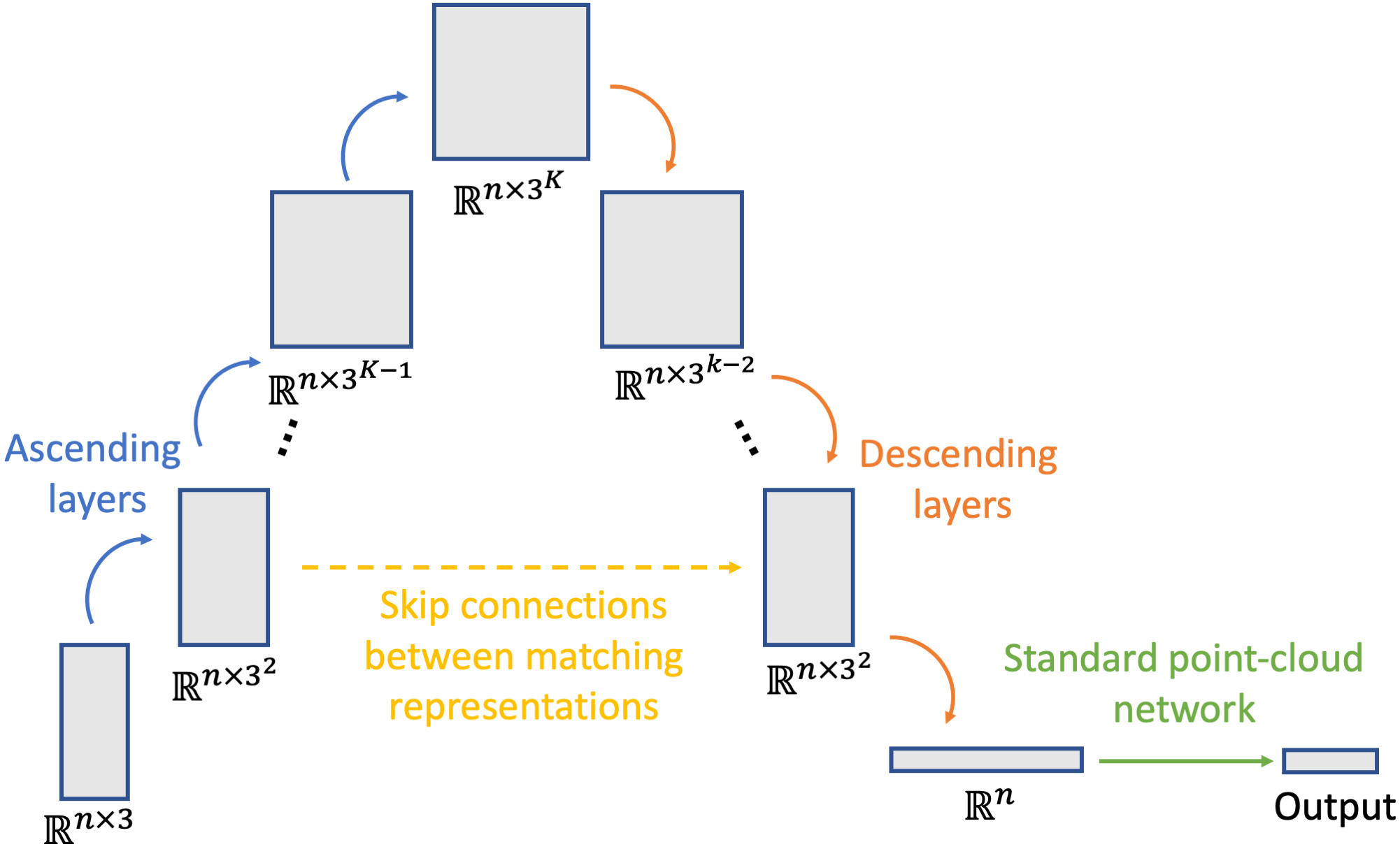
Figure 1: Our architecture ${\mathcal{F}}(K,C)$ with $C=1$.

The architecture we use depends on two hyper-parameters: the number of channels $C$ (which we keep fixed throughout the network), and the maximal representation order used $K$. This choice of hyper-parameters defines a parametric function space ${\mathcal{F}}(K,C)$, containing functions which gradually map pointclouds up to $K$ order representations, and then gradually map back down, using the ascending, descending and linear layers discussed above. The architecture is visualized in Figure 1 (with $C=1$ and using the identification ${\mathcal{T}}_{k}=\mathbb{R}^{3^{k}}$). We next formally describe our architecture.

We denote the input point cloud by $X\in\mathbb{R}^{3\times n}$, and define an initial degenerate representation $U^{(0)}\in{\mathcal{T}}_{0}^{n\times C}$ which is identically one in all $n\cdot C$ coordinates. we recursively define for $k=1,\ldots,K$

$$U^{(k)}={\mathcal{L}}\left({\mathcal{A}}(U^{(k-1)},X)\right).$$

where we suppress the dependence of ${\mathcal{A}}$ and ${\mathcal{L}}$ on the learned parameters $\bm{\alpha}^{(k)}$ and $\bm{\gamma}^{(k)}$ for notation simplicity. Each $U^{(k)}=U^{(k)}(X)$ contains $n\times C$ copies of a $3^{k}$ dimensional tensor in ${\mathcal{T}}_{k}$. Next we denote $U^{(K)}=V^{(K)}$ and recursively define for $k=K,K-2,\ldots,r+2$ where $r=K(\mod 2)$

$$V^{(k-2)}={\mathcal{L}}\left(concat({\mathcal{D}}(V^{(k)}),U^{(k-2)})\right)$$ (3)

where again we suppress the dependence of ${\mathcal{D}}$ and ${\mathcal{L}}$ on the learned parameters $\bm{\beta}^{(k-2)}$ and $\bar{\bm{\gamma}}^{(k-2)}$ for simplicity. Overall we get a function $f:{\mathcal{T}}_{1}^{n\times C}\to{\mathcal{T}}_{r}^{n\times C}$ of the form

$$V^{(r)}=f(X|\bm{\alpha}^{(1)},\ldots ,\bm{\alpha}^{(K)},\bm{\beta}^{(K-2)},\ldots,\bm{\beta}^{(r)},$$

$$\bm{\gamma}^{(1)},\ldots,\bm{\gamma}^{(K)},\bar{\bm{\gamma}}^{(K-2)},\ldots,\bar{\bm{\gamma}}^{(r)}).$$

The function $f$ is permutation and ortho-equivariant when $r=1$ or ortho-invariant and permutation equivariant when $r=0$. When $r=0$ we can apply a permutation invariant/equivariant network such as PointNet (Qi et al., 2017) or DGCNN (Wang et al., 2019) to the output of our network to strengthen the expressive power of our network while maintaining the ortho-invariance and permutation invariance/equivariance of our overall construction.

Expansion of basic model

The basic model we presented up to now is sufficient to prove universality as discussed in Theorem 3.1 below. However, it is only able to compute polynomials up to degree $K$. To enable expression of non-polynomial functions we use the ReLU activation layer defined in (Deng et al., 2021) (which easily generalizes to higher representations). To take local information into account, we expand our ascending layer in equation 2 by adding a summation over the K-nearest neighbors in feature space, giving

$$V^{out}_{jc} =\alpha_{1c}\left(X_{j}\otimes V_{jc}\right)+\alpha_{2c}\sum_{i\neq j}X_{i}\otimes V_{ic}$$

$$+\alpha_{3c}\sum_{i\sim j}X_{i}\otimes V_{ic}.$$

Finally, we have experimented with adding linear layers which map ${\mathcal{T}}_{k}$ equivariantly to itself. When $k=2$ these linear layers are spanned by the linear mappings

$$V\mapsto V,\,V\mapsto V^{T},\,V\mapsto trace(V)I_{3},\quad V\in{\mathcal{T}}_{2}=\mathbb{R}^{3\times 3}.$$

We find that adding these mappings for $k=2$ improves our results, and generalizing this to higher dimensions is an interesting challenge for further research.

3 Theoretical properties

We now discuss the expressive power of the architecture ${\mathcal{F}}(K,C)$ defined above. Based on the proof methodology of (Dym & Maron, 2020), we prove the following theorem (stated formally in the appendix)

Theorem 3.1.

[non-formal statement] For every even $K$ and large enough $C\geq C(K)$, every polynomial of degree $\leq K$ which is permutation equivariant (or invariant) and invariant to rigid motions can be expressed by functions in ${\mathcal{F}}(K,C)$ composed with simple pooling and centralizing operations.

Since the invariant/equivariant polynomials are dense in the space of continuous invariant functions (uniformly on compact sets, see e.g., Lemma 1 in (Dym & Maron, 2020)) this theorem means that in the limit where $K,C\rightarrow\infty$ our architecture is able to approximate any function invariant to orthogonal transformations, translations and permutations.

A disadvantage of universality theorems is that it is unclear how big a network is needed to get a reasonable approximation of a given function. In Theorem B.3, stated and proved in the appendix, we consider the function $\lambda_{Cov}$ which computes the three eigenvalues of the covariance matrix of the point cloud $X$, ordered according to size. This is a classical global descriptor (see e.g.,(Puny et al., 2021; Kazhdan et al., 2004)) which is invariant to permutations and rigid motions. We show that it can be computed by our networks with representations of order $K=6$, composed with a continuous (non-invariant) function $q$ which can be approximated by an MLP.

4 Experiments

Methods	z/z	z/SO(3)	SO(3)/SO(3)
SFCNN Rao et al. (2019)	91.4	84.8	90.1
TFN Thomas et al. (2018)	88.5	85.3	87.6
RI-Conv Zhang et al. (2019)	86.5	86.4	86.4
SPHNet Poulenard et al. (2019)	87.7	86.6	87.6
ClusterNet Chen et al. (2019)	87.1	87.1	87.1
GC-Conv Zhang et al. (2020)	89.0	89.1	89.2
RI-Framework Li et al. (2021)	89.4	89.4	89.3
VN-PointNet Deng et al. (2021)	77.5	77.5	77.2
VN-DGCNN Deng et al. (2021)	89.5	89.5	90.2
Our method (K=2)	78.3	78.4	77.7
Our method (K=4)	80.4	80.4	78.8
Our method (K=6)	81.6	81.5	80.1
Ours (K=4) w.o. VNReLU (K=4)	51.4	51.4	55.2
Ours (K=4) w.o. VNReLU & KNN (K=4)	35.8	35.8	33.8

Table 1: Test clasification accuracy on the ModelNet40 dataset in three train/test scenarios. z stands for the aligned data augmented by random rotations around the vertical axis and SO(3) indicates data augmented by random rotations. All models presented in the table are rotation and permutation invariant (up to numerical inaccuracies).

In this section, we evaluate our model. In Section 4.1, we describe in details the experimental setup we have used and in Section 4.2 we present our main results.

4.1 Experimental Setting

Data

We evaluated our proposed network on a standard point cloud classification benchmark, ModelNet40 (Wu et al., 2015), which consists of 40 classes with 12,311 pre-aligned CAD models, split into 80% for training and 20% for testing. Classification problems are invariant to rigid motions and permutations. We preprocess the point cloud to have zero mean to achieve translation invariance, and then apply the model described in the paper with $K$ even to achieve function invariant to rigid motions and equivariant to permutations. Finally we apply sum pooling and a fully connected neural network to achieve a fully invariant model.

Implementation

We trained and tested our model on NVidia GTX A6000 GPUs with python 3.9, Cuda 11.3, PyTorch 1.10.0, PyTorch geometric, and pytorch3d 0.6.0. We trained our model for 100 epochs with a batch size of 32, a learning rate of 0.1, and a seed of 0.

4.2 Experimental Results

We present initial results of our model on the ModelNet40 classification task, under the three standard evaluation protocols for jointly equivariant architectures: in the first protocol (z/z) train and test data are augmented with rotations around the z-axis, in the second (z/SO(3)) train data is augmented by rotations around the z-axis and test data is augmented by general 3D rotations, and in the third protocol (SO(3)/SO(3)) train and test data are augmented by 3D rotations.

We compared our method to SFCNN (Rao et al., 2019), TFN (Thomas et al., 2018), RI-Conv (Zhang et al., 2019), SPHNet (Poulenard et al., 2019), ClusterNet (Chen et al., 2019), GC-Conv (Chen et al., 2019), RI-Framework (Li et al., 2021) and to two variations of Vector Neurons (Deng et al., 2021). The results of the comparison are shown in Table 1. In general We find that our model does not perform as well as many of the models we compared too.

All methods we compared to, as well as our own method, are invariant to rigid motions and permutations, and as a result are hardly effected when the test data is augmented by general 3D rotations (z/SO(3)) or when both test and train are augmented by 3D rotations (SO(3)/SO(3)) (for comparison, see the results for the three augemntation protocols obtained for methods without rotation invariance, as shown e.g., in (Deng et al., 2021)).

Ablation on our method

We examine the contribution of high representations by comparing different representation orders $K=2,4,6$. As expected we find that higher representation lead to better accuracy. Without the use of the ReLU activation layer defined in (Deng et al., 2021), the accuracy of our method decreases by 29.0%. When we remove the K-nearest neighbors summation as well, the accuracy of our method decreases by an additional 15.6%.

5 Conclusion and future work

In this short paper we first presented an implementation of a simple, universal, neural network architecture which is jointly equivariant of permutations and rigid motions. Experimentally, we find that our model does not perform as well as recent state of the art architectures with joint permutation and rigid motion invariance. We are currently working on additional expansions to our basic model, such as the study of equivariant linear mappings on ${\mathcal{T}}_{k}$ mentioned above, and believe this may lead to improved results on Modelnet40 and other equivariant learning tasks.

At the same time, we believe the inability of our method, as well as other semi-lifted approaches such as TFN, to outperform methods with low-dimensional representations is worthy of further study and raises many interesting questions for further reseach. For example: Are the low dimensional models universal? If they aren’t, what equivariants tasks are they likely to fail in? Is there an explanation to their successfulness in other tasks? Is it possible that semi-lifted models are more expressive but are difficult to optimize? If so can this difficulty be alleviated? We hope to address these questions in future work, and hope others will be inspired to do the same.

Appendix A Equivariance proofs

We begin by proving

Proposition A.1.

Tensor products and contractions are ${\mathcal{O}}(3)$ equivariant.

As a preliminary to this proof, recall that $T\in{\mathcal{T}}_{k}$ is a rank one tensor if there exists $t^{(1)},\ldots,t^{(k)}\in\mathbb{R}^{3}$ such that

$$T_{k}=t^{(1)}\otimes t^{(2)}\otimes\ldots\otimes t^{(k)}.$$ (4)

Proof of Proposition A.1.

equivariance of tensor products

We need to show that for $T\in{\mathcal{T}}_{k}$ and $S\in{\mathcal{T}}_{\ell}$ we have

$$R^{\otimes k}T\otimes R^{\otimes\ell}S=R^{\otimes(k+\ell)}\left(T\otimes S\right),\quad\forall R\in{\mathcal{O}}(3).$$ (5)

since both sides of the equation are bilinear in $(T,S)$, and since every tensor in ${\mathcal{T}}_{k}$ can be written as a linear combination of rank one tensors, it is sufficient to prove equation 5 for the special case where $T$ and $S$ are rank one tensors. If $T$ is a rank one tensor as in equation 4, then $R^{\otimes k}T$ is given by

$$\left[(Rt^{(1)})\otimes(Rt^{(2)})\otimes\ldots\otimes(Rt^{(k)})\right]_{i_{1},\ldots,i_{k}} =(Rt^{(1)})_{i_{1}}\times(Rt^{(2)})_{i_{2}}\times\ldots\times(Rt^{(k)})_{i_{k}}$$

$$=\left(\sum_{j_{1}=1}^{3}R_{i_{1}j_{1}}t_{j_{1}}^{(1)}\right)\left(\sum_{j_{2}=1}^{3}R_{i_{2}j_{2}}t_{j_{2}}^{(2)}\right)\ldots\left(\sum_{j_{k}=1}^{3}R_{i_{k}j_{k}}t_{j_{k}}^{(k)}\right)$$

$$=\sum_{j_{1},\ldots,j_{k}=1}^{3}R_{i_{1},j_{1}}R_{i_{2},j_{2}}\ldots R_{i_{k},j_{k}}T_{j_{1},j_{2},\ldots,j_{k}}$$

$$=\left(R^{\otimes k}T\right)_{i_{1},\ldots,i_{k}}$$

it follows that for every rank one tensors $T=t^{(1)}\otimes t^{(2)}\otimes\ldots\otimes t^{(k)}$ and $S=s^{(1)}\otimes s^{(2)}\otimes\ldots\otimes s^{(\ell)}$ we have for every $R\in{\mathcal{O}}(3)$

$$R^{\otimes k}T\otimes R^{\otimes\ell}S =(Rt^{(1)})\otimes(Rt^{(2)})\otimes\ldots\otimes(Rt^{(k)})\otimes(Rs^{(1)})\otimes(Rs^{(2)})\otimes\ldots\otimes(Rs^{(\ell)})$$

$$=R^{\otimes(k+\ell)}\left[t^{(1)}\otimes t^{(2)}\otimes\ldots\otimes t^{(k)}\otimes s^{(1)}\otimes s^{(2)}\otimes\ldots\otimes s^{(\ell)}\right]$$

$$=R^{\otimes(k+\ell)}(T\otimes S)$$

and thus we have shown correctness of equation 5 for all rank-one tensors and thus for all tensors. We note that this proof does not really require $R$ to be an orthogonal matrix and would work for any square matrix. This is not the case for contractions, as we will see next:

equivariance of contractions For simplicity of notation we prove the equivariance of contractions $C_{a,b}:{\mathcal{T}}_{k}\to{\mathcal{T}}_{k-2}$ in the special case $a=k-1,b=k$. We need to show that for all $T\in{\mathcal{T}}_{k}$ and $R\in{\mathcal{O}}(3)$ we have

$$C_{k-1,k}(R^{\otimes k}T)=R^{\otimes(k-2)}C_{k-1,k}(T)$$ (6)

since both sides of the equation above are linear in $T$ and every tensor of order $k$ can be written as a linear combination of rank one tensors, it is sufficient to show that equation 6 holds for all rank one tensors. Let $T$ be a rank one tensor as in equation 4. Note that by definition

$$\left[C_{k-1,k}(T)\right]_{i_{1},i_{2},\ldots,i_{k-2}} =\sum_{j=1}^{3}T_{i_{1},\ldots,i_{k-2},j,j}$$ (7)

$$=\langle t^{(k-1)},t^{(k)}\rangle\left[t^{(1)}\otimes t^{(2)}\otimes\ldots\otimes t^{(k-2)}\right]$$

and so for every $R\in{\mathcal{O}}(3)$, since we saw in the first part of the proof that $R^{\otimes k}T$ is a rank one tensor given by

$$R^{\otimes k}T=(Rt^{(1)})\otimes(Rt^{(2)})\otimes\ldots\otimes(Rt^{(k)})$$

and so we get that

$$C_{k-1,k}(R^{\otimes k}T) =\langle Rt^{(k-1)},Rt^{(k)}\rangle(Rt^{(1)})\otimes(Rt^{(2)})\otimes\ldots(Rt^{(k)})$$

$$=\langle t^{(k-1)},t^{(k)}\rangle(Rt^{(1)})\otimes(Rt^{(2)})\otimes\ldots(Rt^{(k)})$$

$$=\langle t^{(k-1)},t^{(k)}\rangle\left[R^{\otimes(k-2)}\left(t^{(1)}\otimes t^{(2)}\otimes\ldots\otimes t^{(k-2)}\right)\right]$$

$$=R^{\otimes(k-2)}C_{k-1,k}(T).$$

Thus we have shown that equation 6 holds for all rank one tensors and thus for all tensors. This concludes the prove of Proposition A.1. ∎

Layer equivariance We now prove equivariance of our layers. In the following discussion we use the notation $\rho_{k}(R,\sigma)$ for the action of $(R,\sigma)$ on ${\mathcal{T}}_{k}^{n\times C}$ as defined in equation 1.

Proposition A.2.

For any choice of parameters, the layers ${\mathcal{A}},{\mathcal{D}}$ and ${\mathcal{L}}$ are equivariant.

Proof of Proposition A.2.

Equivariance of ascending layers We need to show that for every given input $X\in\mathbb{R}^{3\times n},V\in{\mathcal{T}}_{k}^{n\times C}$, for every $R\in{\mathcal{O}}(3),\sigma\in S_{n}$ and any fixed parameter vector $\bm{\alpha}$

$$\rho_{k+1}(R,\sigma)V^{out}={\mathcal{A}}(\rho_{k}(R,\sigma)V^{in},\rho_{1}(R,\sigma)X|\bm{\alpha})$$

Indeed using the definition of the action $\rho_{k+1}$ from equation 1 and the equivariance of the tensor prouct we proved above, we have

$$\left[\rho_{k+1}(R,\sigma)V^{out}\right]_{jc} =R^{\otimes(k+1)}[V^{out}_{\sigma^{-1}(j),c}]$$

$$=\alpha_{1c}R^{\otimes(k+1)}\left(X_{\sigma^{-1}(j)}\otimes V_{\sigma^{-1}(j)c}\right)+\alpha_{2c}\sum_{i\neq\sigma^{-1}(j)}R^{\otimes(k+1)}\left(X_{i}\otimes V_{ic}\right)$$

$$=\alpha_{1c}(RX_{\sigma^{-1}(j)})\otimes(R^{\otimes k}V_{\sigma^{-1}(j)c})+\alpha_{2c}\sum_{i\neq\sigma^{-1}(j)}(RX_{i})\otimes(R^{\otimes k}V_{ic})$$

$$=[{\mathcal{A}}(\rho_{k}(R,\sigma)V^{in},\rho_{1}(R,\sigma)X|\bm{\alpha})]_{j,c}$$

Equivariance of descending layers We need to show that for all $R\in{\mathcal{O}}(3),\sigma\in S_{n}$, for all $V^{in}\in{\mathcal{T}}_{k}^{n\times C},V^{out}\in{\mathcal{T}}_{k-2}^{n\times C}$ and for all choice of a parameter vector $\bm{\beta}$,

$$\rho_{k-2}(R,\sigma)V^{out}={\mathcal{D}}(\rho_{k}(R,\sigma)V^{in}|\bm{\beta}).$$

Using the definition of the action $\rho_{k}$ from equation 1 and the equivariance of contraction we proved above, we have

$$[\rho_{k-2}(V^{out})]_{j,c} =R^{\otimes(k-2)}[V^{out}_{\sigma^{-1}(j),c}]=\sum_{1\leq a<b\leq k}\beta_{a,b,c}R^{\otimes(k-2)}C_{a,b}(V^{in}_{\sigma^{-1}(j),c})$$

$$=\sum_{1\leq a<b\leq k}\beta_{a,b,c}C_{a,b}(R^{\otimes k}V^{in}_{\sigma^{-1}(j),c})=[{\mathcal{D}}(\rho_{k}(R,\sigma)V^{in}|\bm{\beta})]_{j,c}$$

Equivariance of linear layers

We need to show that for all $R\in{\mathcal{O}}(3),\sigma\in S_{n}$, for all $V^{in},V^{out}\in{\mathcal{T}}_{k}^{n\times C}$ and for all choice of a parameter vector $\bm{\gamma}$,

$$\rho_{k}(R,\sigma)V^{out}={\mathcal{L}}(\rho_{k}(R,\sigma)V^{in}|\bm{\gamma}).$$

Indeed

$$[\rho_{k}(R,\sigma)V^{out}]_{jc^{\prime}} =R^{\otimes k}[V^{out}_{\sigma^{-1}(j),c^{\prime}}]=\sum_{c=1}^{C}\gamma_{cc^{\prime}}R^{\otimes k}V_{\sigma^{-1}(j)c}^{in}$$

$$=[{\mathcal{L}}(\rho_{k}(R,\sigma)V^{in}|\bm{\gamma})]_{jc^{\prime}}.$$

This concludes the prove of Proposition A.2. ∎

Appendix B Expressive power proofs

We now reformulate and prove Theorem 3.1.

Theorem B.1 (Reformulation of Theorem 3.1).

For every even number $K$ and every large enough $C=C(K)$, every polynomial $p:\mathbb{R}^{3\times n}\to\mathbb{R}^{n}$ of degree $\leq K$ which is permutation equivariant and invariant to rigid motions can be obtained as the first channel of a function $f\in{\mathcal{F}}(K,C)$, that is

$$p_{j}(X)=f_{j1}(X),\forall j=1,\ldots,n$$

This immediately implies an analogous result where we replace the permutation equivariant assumption by a permutation invariant assumption:

Corollary B.2.

For every even number $K$ and every large enough $C=C(K)$, every polynomial $p:\mathbb{R}^{3\times n}\to\mathbb{R}$ of degree $\leq K$ which is invariant to permutations and rigid motions can be obtained by applying sum pooling to the first channel of a function $f\in{\mathcal{F}}(K,C)$, that is

$$p(X)=\sum_{j=1}^{n}f_{j1}(X-\frac{1}{n}X1_{n}1_{n}^{T})$$

proof of Theorem 3.1.

Our proof is based on the general framework for proving universality laid out in (Dym & Maron, 2020). In this paper it is shown that polynomials $p:\mathbb{R}^{3\times n}\to\mathbb{R}^{n}$ of degree $K$ which are permutation equivariant and invariant to translations and orthogonal transformationscan be written for large enough $C$ as

$$p(X)=\sum_{c=1}^{C}\hat{\Lambda}_{c}\left(g_{c}(X)\right)$$ (8)

where

1. $g_{c}$ is a member of a function space ${\mathcal{F}}_{\mathrm{feat}}$ which maps $\mathbb{R}^{3\times n}$ to $W_{\mathrm{feat}}^{n}$, where $W_{\mathrm{feat}}$ is a representation of ${\mathcal{O}}(3)$.

2. $\Lambda_{c}$ is a member of a space of functions ${\mathcal{F}}_{\mathrm{pool}}$ from $W_{\mathrm{feat}}$ to $\mathbb{R}$ and $\hat{\Lambda}_{c}:W_{\mathrm{feat}}^{n}\to\mathbb{R}^{n}$ is the function induced by elementwise application of $\Lambda_{c}$.

3. The function spaces ${\mathcal{F}}_{\mathrm{pool}}$ has the linear universality property. This means that ${\mathcal{F}}_{\mathrm{pool}}$ is precisely the set of linear functionals $\Lambda:W_{\mathrm{feat}}\to\mathbb{R}$ which are ${\mathcal{O}}(3)$ equivariant.

4. the function space ${\mathcal{F}}_{\mathrm{feat}}$ has the $K$-spanning property. This means that all functions in ${\mathcal{F}}_{\mathrm{feat}}$ are required to by ${\mathcal{O}}(3)\times S_{n}$ equivaraint and invariant to translations, and additionally, that any permutation equivariant and translation invariant (ortho-equivariance not required) degree $D$ polynomial $\tilde{p}:\mathbb{R}^{3\times n}\to\mathbb{R}^{n}$ can be obtained by an expression as in equation 8 where $\Lambda_{c}$ are linear but are not required to be ortho-invariant.

It is also shown in Lemma 3 in (Dym & Maron, 2020) that the spaces of functions obtained by applying ascending layers recursively $k=1,\ldots,K$ times form a $K$-spanning family. Here we use ascending layers independently on each channel and essentially remove the linear layers by setting $\bm{\gamma}^{(k)}_{cc^{\prime}}=\delta_{cc^{\prime}}$ for all $k=1,\ldots,K$. Applying ascending layers $k$ times gives us a function from $\mathbb{R}^{3\times n}$ to ${\mathcal{T}}_{k}$, and since we are basically considering a collection of different functions to different representations ${\mathcal{T}}_{1},\ldots,{\mathcal{T}}_{K}$ (depending on the number of ascending layers used) we choose to embed all these representations into a joint representation $W_{\mathrm{feat}}=\oplus_{k=1}^{K}{\mathcal{T}}_{k}$. Thus we see that every permutation equivaraint and translation and ortho-invariant polynomial $p$ can be written in the form equation 8 where the $g_{c}$ are obtained by applying our ascending layers $k_{c}$ times for some $1\leq k_{c}\leq K$ and $\Lambda_{c}:\oplus_{k=1}^{K}{\mathcal{T}}_{k}\to\mathbb{R}$ is linear and ortho-invariant. Since $g_{c}$ maps into a single representation ${\mathcal{T}}_{k_{c}}$ in practice we can think of $\Lambda_{c}$ is a linear equivariant functional on this single representation.

Using an analogous argument to the proof of Proposition 1 in Appendix 5 in (Dym & Maron, 2020), it can be shown that the space of linear invariant functionals $\Lambda:{\mathcal{T}}_{k}\to\mathbb{R}$ are spanned by the functionals $\{\Lambda_{\sigma}|\,\sigma\in S_{k}\}$ which are defined uniquely be the requirement that for every $x^{(1)},\ldots,x^{(k)}\in\mathbb{R}^{3}$,

$$\Lambda_{\sigma}(x^{\sigma(1)})\otimes\ldots\otimes x^{\sigma(k)})=\langle x^{\sigma(1)},x^{\sigma(2)}\rangle\times\langle x^{\sigma(3)},x^{\sigma(4)}\rangle\ldots\langle x^{\sigma(k-1)},x^{\sigma(k)}\rangle.$$

These $\Lambda_{\sigma}$ are given by (see also the derivation of equation 7)

$$\Lambda_{\sigma}(T)=C_{\sigma(1),\sigma(2)}\circ C_{\sigma(3),\sigma(4)}\circ\ldots\circ C_{\sigma(k-1),\sigma(k)}(T).$$

In particular we see that if $k$ is odd there is no non-zero linear equivariant functional from ${\mathcal{T}}_{k}$ to $\mathbb{R}$, so we can assume that $k_{c}$ is even for all $c=1,\ldots,C$, and $\Lambda_{c}$ can be obtained by applying the last $k_{c}/2$ descending layers of our construction to the output $U^{(k_{c})}$ of $g_{c}$ with an appropriate choice of $0-1$ parameters. Recall that $U^{(k_{c})}=g_{c}(X)$ was obtained from $k_{c}$ ascending layers. When $k_{c}<K$ we achieve this using our $K$-dimensional $U$-shaped architecture by ‘short-circuiting’ at the $k_{c}$ level, that is by setting the parameters of the linear layer ${\mathcal{L}}$ in equation 3 to erase ${\mathcal{D}}(U^{(k_{c}+2)})$ and maintain only $U^{(k_{c})}$.

We have seen that we can write $p$ as in equation 8 where $\hat{\Lambda}_{c}$ and $g_{c}$ can be constructed to be the $c$-th channel of our network. We obtain the sum of $\hat{\Lambda}_{c}\circ g_{c}$ in the first channel of the output representation $V^{(0)}$ by setting the first column of the parameter matrix $\bm{\gamma}^{(0)}$ of the last linear layer
to be $\gamma_{c1}^{(0)}=1,\forall c=1,\ldots,C$ .

∎

Computing eigenvalues of the covariance matrix We prove

Theorem B.3.

Let $\lambda_{Cov}:\mathbb{R}^{3\times n}\to\mathbb{R}^{3}$ be the function which, given a point cloud $X\in\mathbb{R}^{3\times n}$, computes the ordered eigenvalues of the covariance matrix $(X-\frac{1}{n}X1_{n}1_{n}^{T})(X-\frac{1}{n}X1_{n}1_{n}^{T})^{T}$. For large enough $C$ there exists $f\in{\mathcal{F}}(6,C)$ and a continuous $q:\mathbb{R}^{3}\to\mathbb{R}^{3}$ such that

$$\lambda_{Cov}(X)=q\left(\sum_{j=1}^{n}f_{j1}(X-\frac{1}{n}X1_{n}1_{n}^{T}),\sum_{j=1}^{n}f_{j2}(X-\frac{1}{n}X1_{n}1_{n}^{T}),\sum_{j=1}^{n}f_{j3}(X-\frac{1}{n}X1_{n}1_{n}^{T})\right)$$

proof of Theorem B.3.

The covariance matrix of $X\in\mathbb{R}^{3\times n}$ is given by

$$\bar{X}{\bar{X}}^{T}\text{, where }\bar{X}=X-\frac{1}{n}1_{n}1_{n}^{T}.$$

The covariance matrix is a symmetric positive semi-definite matrix and we denote its eigenvalues by $\lambda_{1}(X)\geq\lambda_{2}(X)\geq\lambda_{3}(X)\geq 0$ and define

$$\lambda_{Cov}(X)=(\lambda_{1}(X),\lambda_{2}(X),\lambda_{3}(X))$$

We now define polynomials $p_{2},p_{4},p_{6}$ of degree $2,4,6$ which are invariant to permutations and rigid motions, by

$$p_{2}(X) =\operatorname{Tr}(\bar{X}{\bar{X}}^{T})=\lambda_{1}(X)+\lambda_{2}(X)+\lambda_{3}(X)$$

$$p_{4}(X) =\operatorname{Tr}(\left(\bar{X}{\bar{X}}^{T}\right)^{2})=\lambda_{1}^{2}(X)+\lambda_{2}^{2}(X)+\lambda_{3}^{2}(X)$$

$$p_{6}(X) =\operatorname{Tr}(\left(\bar{X}{\bar{X}}^{T}\right)^{3})=\lambda_{1}^{3}(X)+\lambda_{2}^{3}(X)+\lambda_{3}^{3}(X)$$

Since $p_{2},p_{4},p_{6}$ are invariant and of degree $\leq 6$ we can approximated them with our architecture ${\mathcal{F}}(6,C)$ with $C$ large enough.

It remains to show that there exists a continuous mapping $q:\mathbb{R}^{3}\to\mathbb{R}^{3}$ such that (dropping the dependence of the eigenvalues on $X$)

$$q\left(\lambda_{1}+\lambda_{2}+\lambda_{3},\lambda_{1}^{2}+\lambda_{2}^{2}+\lambda_{3}^{2},\lambda_{1}^{3}+\lambda_{2}^{3}+\lambda_{3}^{3}\right)=(\lambda_{1},\lambda_{2},\lambda_{3})$$

This follows from the fact that the three polynomials $s_{1},s_{2},s_{3}:\mathbb{R}^{3}\to\mathbb{R}$

$$s_{1}(\lambda_{1},\lambda_{2},\lambda_{3}) =\lambda_{1}+\lambda_{2}+\lambda_{3}$$

$$s_{2}(\lambda_{1},\lambda_{2},\lambda_{3}) =\lambda_{1}^{2}+\lambda_{2}^{2}+\lambda_{3}^{2}$$

$$s_{3}(\lambda_{1},\lambda_{2},\lambda_{3}) =\lambda_{1}^{3}+\lambda_{2}^{3}+\lambda_{3}^{3}$$

are permutation invariant polynomials known as the power sum polynomials, which generate the ring of permutation invariant polynomials on $\mathbb{R}^{3}$, and as such, the map $\bm{s}=(s_{1},s_{2},s_{3})$ induces a homeomorphism of $\mathbb{R}^{3}/S_{3}$ onto the image of $\bm{s}$ ((González & de Salas, 2003), Lemma 11.13) . Similarly, the sorting function $\mathrm{sort}:\mathbb{R}^{3}\to\mathbb{R}^{3}$ is an injective permutation invariant mapping which induces a homeomorphism of $\mathbb{R}^{3}/S_{3}$ onto its image. Thus the sets

$$\{\bm{s}(\lambda_{1},\lambda_{2},\lambda_{3})|\,(\lambda_{1},\lambda_{2},\lambda_{3})\in\mathbb{R}^{3}\}\text{ and }\{\mathrm{sort}(\lambda_{1},\lambda_{2},\lambda_{3})|\,(\lambda_{1},\lambda_{2},\lambda_{3})\in\mathbb{R}^{3}\}$$

are homeomorphic, and we can choose $q$ to be a homeomorphism (in particular, $q$ is continuous). ∎

References

- Babai (2016) Babai, L. Graph isomorphism in quasipolynomial time. In Proceedings of the forty-eighth annual ACM symposium on Theory of Computing, pp. 684–697, 2016.
- Bogatskiy et al. (2020) Bogatskiy, A., Anderson, B., Offermann, J., Roussi, M., Miller, D., and Kondor, R. Lorentz group equivariant neural network for particle physics. In International Conference on Machine Learning, pp. 992–1002. PMLR, 2020.
- Bökman et al. (2021) Bökman, G., Kahl, F., and Flinth, A. Zz-net: A universal rotation equivariant architecture for 2d point clouds. arXiv preprint arXiv:2111.15341, 2021.
- Chen et al. (2019) Chen, C., Li, G., Xu, R., Chen, T., Wang, M., and Lin, L. Clusternet: Deep hierarchical cluster network with rigorously rotation-invariant representation for point cloud analysis. In 2019 IEEE/CVF Conference on Computer Vision and Pattern Recognition (CVPR), pp. 4989–4997, 2019. doi: 10.1109/CVPR.2019.00513.
- Deng et al. (2021) Deng, C., Litany, O., Duan, Y., Poulenard, A., Tagliasacchi, A., and Guibas, L. J. Vector neurons: A general framework for so (3)-equivariant networks. In Proceedings of the IEEE/CVF International Conference on Computer Vision, pp. 12200–12209, 2021.
- Dym & Lipman (2017) Dym, N. and Lipman, Y. Exact recovery with symmetries for procrustes matching. SIAM Journal on Optimization, 27(3):1513–1530, 2017.
- Dym & Maron (2020) Dym, N. and Maron, H. On the universality of rotation equivariant point cloud networks. arXiv preprint arXiv:2010.02449, 2020.
- Fuchs et al. (2020) Fuchs, F., Worrall, D., Fischer, V., and Welling, M. Se (3)-transformers: 3d roto-translation equivariant attention networks. Advances in Neural Information Processing Systems, 33:1970–1981, 2020.
- Gilmer et al. (2017) Gilmer, J., Schoenholz, S. S., Riley, P. F., Vinyals, O., and Dahl, G. E. Neural message passing for quantum chemistry. In International conference on machine learning, pp. 1263–1272. PMLR, 2017.
- González & de Salas (2003) González, J. A. N. and de Salas, J. B. S. -differentiable spaces, volume 1824. Springer, 2003.
- Kazhdan et al. (2004) Kazhdan, M., Funkhouser, T., and Rusinkiewicz, S. Shape matching and anisotropy. In ACM SIGGRAPH 2004 Papers, pp. 623–629. 2004.
- Klicpera et al. (2021) Klicpera, J., Becker, F., and Günnemann, S. Gemnet: Universal directional graph neural networks for molecules. Advances in Neural Information Processing Systems, 34, 2021.
- Kondor et al. (2018) Kondor, R., Son, H. T., Pan, H., Anderson, B., and Trivedi, S. Covariant compositional networks for learning graphs. arXiv preprint arXiv:1801.02144, 2018.
- Li et al. (2021) Li, X., Li, R., Chen, G., Fu, C.-W., Cohen-Or, D., and Heng, P.-A. A rotation-invariant framework for deep point cloud analysis. IEEE Transactions on Visualization and Computer Graphics, pp. 1–1, 2021. ISSN 2160-9306. doi: 10.1109/tvcg.2021.3092570. URL http://dx.doi.org/10.1109/TVCG.2021.3092570.
- Maron et al. (2018) Maron, H., Ben-Hamu, H., Shamir, N., and Lipman, Y. Invariant and equivariant graph networks. arXiv preprint arXiv:1812.09902, 2018.
- Maron et al. (2019a) Maron, H., Ben-Hamu, H., Serviansky, H., and Lipman, Y. Provably powerful graph networks. Advances in neural information processing systems, 32, 2019a.
- Maron et al. (2019b) Maron, H., Fetaya, E., Segol, N., and Lipman, Y. On the universality of invariant networks. In International conference on machine learning, pp. 4363–4371. PMLR, 2019b.
- Maron et al. (2020) Maron, H., Litany, O., Chechik, G., and Fetaya, E. On learning sets of symmetric elements. In International Conference on Machine Learning, pp. 6734–6744. PMLR, 2020.
- Morris et al. (2019) Morris, C., Ritzert, M., Fey, M., Hamilton, W. L., Lenssen, J. E., Rattan, G., and Grohe, M. Weisfeiler and leman go neural: Higher-order graph neural networks. In Proceedings of the AAAI conference on artificial intelligence, volume 33, pp. 4602–4609, 2019.
- Morris et al. (2021) Morris, C., Lipman, Y., Maron, H., Rieck, B., Kriege, N. M., Grohe, M., Fey, M., and Borgwardt, K. Weisfeiler and leman go machine learning: The story so far. arXiv preprint arXiv:2112.09992, 2021.
- Poulenard et al. (2019) Poulenard, A., Rakotosaona, M.-J., Ponty, Y., and Ovsjanikov, M. Effective rotation-invariant point cnn with spherical harmonics kernels, 2019.
- Puny et al. (2021) Puny, O., Atzmon, M., Ben-Hamu, H., Smith, E. J., Misra, I., Grover, A., and Lipman, Y. Frame averaging for invariant and equivariant network design. arXiv preprint arXiv:2110.03336, 2021.
- Qi et al. (2017) Qi, C. R., Su, H., Mo, K., and Guibas, L. J. Pointnet: Deep learning on point sets for 3d classification and segmentation. In Proceedings of the IEEE conference on computer vision and pattern recognition, pp. 652–660, 2017.
- Rao et al. (2019) Rao, Y., Lu, J., and Zhou, J. Spherical fractal convolutional neural networks for point cloud recognition. In Proceedings of the IEEE/CVF Conference on Computer Vision and Pattern Recognition, pp. 452–460, 2019.
- Ravanbakhsh (2020) Ravanbakhsh, S. Universal equivariant multilayer perceptrons. In International Conference on Machine Learning, pp. 7996–8006. PMLR, 2020.
- Ronneberger et al. (2015) Ronneberger, O., Fischer, P., and Brox, T. U-net: Convolutional networks for biomedical image segmentation. In International Conference on Medical image computing and computer-assisted intervention, pp. 234–241. Springer, 2015.
- Satorras et al. (2021) Satorras, V. G., Hoogeboom, E., and Welling, M. E (n) equivariant graph neural networks. In International Conference on Machine Learning, pp. 9323–9332. PMLR, 2021.
- Thomas et al. (2018) Thomas, N., Smidt, T., Kearnes, S., Yang, L., Li, L., Kohlhoff, K., and Riley, P. Tensor field networks: Rotation-and translation-equivariant neural networks for 3d point clouds. arXiv preprint arXiv:1802.08219, 2018.
- Villar et al. (2021) Villar, S., Hogg, D. W., Storey-Fisher, K., Yao, W., and Blum-Smith, B. Scalars are universal: Equivariant machine learning, structured like classical physics. Advances in Neural Information Processing Systems, 34:28848–28863, 2021.
- Wang et al. (2019) Wang, Y., Sun, Y., Liu, Z., Sarma, S. E., Bronstein, M. M., and Solomon, J. M. Dynamic graph cnn for learning on point clouds. Acm Transactions On Graphics (tog), 38(5):1–12, 2019.
- Wu et al. (2015) Wu, Z., Song, S., Khosla, A., Yu, F., Zhang, L., Tang, X., and Xiao, J. 3d shapenets: A deep representation for volumetric shapes. In Proceedings of the IEEE conference on computer vision and pattern recognition, pp. 1912–1920, 2015.
- Xu et al. (2018) Xu, K., Hu, W., Leskovec, J., and Jegelka, S. How powerful are graph neural networks? arXiv preprint arXiv:1810.00826, 2018.
- Yarotsky (2022) Yarotsky, D. Universal approximations of invariant maps by neural networks. Constructive Approximation, 55(1):407–474, 2022.
- Zaheer et al. (2017) Zaheer, M., Kottur, S., Ravanbakhsh, S., Poczos, B., Salakhutdinov, R. R., and Smola, A. J. Deep sets. Advances in neural information processing systems, 30, 2017.
- Zhang et al. (2019) Zhang, Z., Hua, B.-S., Rosen, D. W., and Yeung, S.-K. Rotation invariant convolutions for 3d point clouds deep learning, 2019.
- Zhang et al. (2020) Zhang, Z., Hua, B.-S., Chen, W., Tian, Y., and Yeung, S.-K. Global context aware convolutions for 3d point cloud understanding, 2020.