Decision-Making Under Uncertainty for Multi-stage Pipelines: Simulation Studies to Benchmark Screening Strategies

Abstract

Multi-stage screening pipelines are ubiquitous throughout experimental and computational science. Much of the effort in developing screening pipelines focuses on improving generative methods or surrogate models in an attempt to make each screening step effective for a specific application. Little focus has been placed on characterizing a generic screening pipeline’s performance with respect to the problem or problem parameters. Here, we develop methods to codify and simulate features and properties about the screening procedure in general. We outline and model common problem settings, and identify potential opportunities to perform decision-making under uncertainty for optimizing the execution of screening pipelines. We then illustrate the developed methods through several simulation studies. We finally show how such studies can provide a quantification of the screening pipeline performance with respect to problem parameters, specifically identifying the significance of stage-wise covariance structure. We show how such structure can lead to qualitatively different screening behaviors, and how screening can even perform worse than random in some cases.

Introduction

Multi-stage screening pipelines are ubiquitous throughout experimental and computational science. In such a pipeline, a set of initial candidates are passed through several evaluative stages. Based on the collective performance of the candidates at any particular stage of the pipeline, a subset of candidates are selected to advance to the next stage; the rest are “screened out”. Typically, this screening is done to minimize how many candidates are evaluated throughout the pipeline, with the goal of identifying promising or optimal candidates with respect to some experimental objective. Often, later stages are more costly, in time, money or other measures of effort.

For example, experimental and virtual screening are used in drug-design [1, 2, 3, 4], chemistry [5], material science[6, 7, 8]. Here, candidate drugs, molecules or materials designs are first tested using preliminary computer models, and promising candidates are then tested in real-world experiments. Another example is multi-modal characterization of materials. In this context, a material sample is characterized using one of several techniques, from atomic force microscopy available in many labs, to X-ray scattering at a synchrotron. Here, a materials scientist may employ an ad hoc screening procedure to identify which materials sample candidates are passed through this characterization pipeline. As autonomous materials platforms begin to incorporate more complex experimental or hybrid computational/experimental structure [9, 10, 11], understanding how screening pipelines could operate in an autonomous manner could allow such platforms the ability to make optimal screening pipeline decisions as well.

The use of a screening procedure relies on a heuristic belief that the screening pipeline will effectively narrow down a search space to a small set of promising leads. But there is no generic guarantee this will work. Consider, for example the case of identifying promising drugs, where the “gold-standard” measure for effectiveness occurs at the last stage of a screening pipeline, which could be performing physical trials of the drug. Imagine the first stage is a machine learning (ML) model meant to predict this effectiveness based on a candidate drug’s descriptors, but its predictions are only slightly correlated or even anti-correlated with the gold-standard measure. In this case, the first stage of the pipeline may aggressively and prematurely screen out good candidates.

To mitigate against this threat, much of the development around screening pipelines has been the development of stages and models that are more strongly correlated to the experimental objectives, either through better surrogate models[12, 13, 14, 15] or through better generative models[16, 17, 18] that determine the initial candidate pool to begin with. Yet fundamental and generic questions persist: What aspects of a problem make the screening procedure effective? Can we quantify the effectiveness of the screening procedure? How do we deal with the uncertainties behind the relationships between stages? Are our current pipeline strategies or ad hoc decision-making policies sufficient in executing an effective pipeline? Coming back to the drug-design example above, we may wish to quantify how poorly the screening procedure performs as a function of the anti-correlation between the first and final stages.

To answer such questions, we must develop a theory where the general pipeline itself is the subject of study, specifically from a perspective of uncertainty quantification and decision-making under uncertainty. In this paper we outline a formalization of a family of screening pipeline problems, and simulation-based policies that we use to make decisions before and during the screening procedure. To accomplish this, we build a model of statistical structure between candidates and stages, and offer algorithms for efficient simulation-based decision-making based on the assumed statistical structure model. Lastly, we present some simulation results to illustrate how such models, simulations, and policies can be used to characterize and optimize screening pipelines.

Problem Definitions

We consider a screening procedure with $m$ initial sampled candidates, $x_{1},x_{2},...,x_{m}$. These candidates can represent drugs, molecules, materials, or even synthesis recipes. Often, these initial candidates are obtained via generative models, ensemble methods, or evolutionary techniques – methods capable of proposing a batch of candidates to test.

We will also consider $n$ stages $f_{1},f_{2},..,f_{n}$, which we shall view as functions mapping candidates $x_{i}$ to corresponding scalar quantities of interest $Y_{i,j}=f_{j}(x_{i})$ as measured by the $j$-th stage. For example in drug design, the stages could represent molecular property predictors, docking score calculations, density functional theory or molecular dynamics simulations, or physical trials. The outcomes for these stages could be computed binding efficacy, free energy calculations, or measures toxicity and synthesizability. In manufacturing, the stages could include low and high fidelity finite element simulations, rapid physical prototyping via 3D printers, and fabrication of a final deliverable. The outcomes for these stages could be measures of mechanical toughness or resiliency.

In the abstract, we call these values scores, so that $Y_{i,j}$ is the score assigned to candidate $x_{i}$ at stage $j$. We interpret these scores as the averaged ground truth values. That is, if we were to repeatedly evaluate a candidate $x_{i}$ through the $j$-th stage, the average of the set of obtained scores will approach the number $Y_{i,j}$. Thus the $Y_{i,j}$ represents the score of candidate $x_{i}$ through the $j$-th stage, averaging over noise or any inherent randomness implicit in making the appropriate measurement and obtaining the quantity of interest.

Throughout, we assume we do not know the scores prior to evaluating the candidates through each stage. As a priori uncertain quantities, we treat the scores within a Bayesian context by modeling such scores using a multivariate probability distribution. That is, throughout the screening procedure, we can maintain a probability distribution for the scores $Y_{i,j}$ that captures predicted estimates of scores not yet evaluated as well as an uncertainty quantification of those predictions and an estimated correlation between different scores. As more data is obtained through the screening procedure, we can update this probability distribution through Bayes’s Law.

Objectives

These scores allow us to define two objectives. First is stage-wise multi-fidelity optimization, in which we view each stage as measuring the same quantity, but with variable accuracies (i.e. fidelities) and costs. In general, we will assume that the last stage $f_{n}$ is the ground-truth or gold-standard that we ultimately care about and is the most expensive. The prior stages exist to perform cheaper screening of candidates. For example, $f_{n}$ could be performing a real experiment, while prior stages could be a sequence of increasingly accurate (and increasingly costly) simulations. A common pipeline in this setting consists of three stages: $f_{1}$ is an ML model, $f_{2}$ is a physics-based simulation, while $f_{3}$ is a physical experiment. Each stage could produce as an output some figure of merit, such as some material property to optimize, and the goal is to find the candidate that optimizes this property in the real-life experiment. Another similar setting is when stages correspond to different materials characterization methods, where the final such method could be an costly trip to a beamline. The stage-wise multi-fidelity optimization problem shall be the main focus of this paper.

Another objective is stage-wise multi-objective optimization. In this setting, we view each stage as characterizing different quantities of interest. For any given candidate $x_{i}$, the scores $Y_{i,1},Y_{i,2},...,Y_{i,n}$ encode a set of different characterizations of candidate $x_{i}$’s material properties or structure, for example. Under the multi-objective objective, we want to identify those candidates $x$ that either 1) optimize some scalar utility $u(x)=u(f_{1}(x),f_{2}(x),...,f_{n}(x))$, or 2) lie on the $n$-dimensional Pareto frontier[19].

Both objectives can be characterized by defining the final reward obtained at the end of the screening procedure. For any screening procedure we obtain a subset $\mathcal{X}_{S}\subseteq\left\{x_{i}\right\}_{i=1}^{m}$ of candidates that “survived” the screening process. For the multi-fidelity objective, we may define the reward as the maximum of the final scores for all such screened candidates, $R=\max_{\mathcal{X}_{S}}f_{m}(x)$. For multi-objective optimization, the final score could be either the maximum scalar utility over all surviving candidates, $R=\max_{\mathcal{X}_{S}}u(x)$, or some measure of improvement to the Pareto front, such as a hypervolume improvement[20], $R=H(\mathcal{X}_{S})-H_{0}.$ Here $H(\mathcal{X}_{S})$ and $H_{0}$ are respectively the hypervolumes defined by the Pareto front generated by the surviving points $\mathcal{X}_{s}$ and prior data points, and the Pareto front obtained from just the prior data points.

Pipeline policies for the optimal allocation design problem

Regardless of how we define the reward, the goal in executing the pipeline is to do so in a way that maximizes the realized reward on average. Throughout, we shall refer to how we execute the pipeline as a pipeline policy. The specific decisions we make during the execution of the pipeline will ultimately impact the rewards we gain at the end of the pipeline. Examples of such decisions include: 1) how many or what proportion of candidates may pass from one stage to the next, 2) how costly each stage is (to the extent that this cost is possible to tune) and 3) how many or which initial candidates do we generate.

In this paper, we shall decompose a pipeline policy into two policies. The inter-stage policy selects which candidates pass to the next stage based on the scores they receive at the current stage. In contrast, the pipeline meta-policy select hyperparameters and constraints that the inter-stage policy must satisfy. The main example used throughout this paper is selecting an allocation $\mathbf{m}=(m_{1},...,m_{n})$ via a meta-policy. An allocation specifies how many candidates are evaluated at each stage. In this notation, $m_{1}=m$ candidates are evaluated in the first stage, then $m_{2}$ candidates are selected (by the inter-stage policy) for the second stage, and so on. Throughout, we require each stage to screen out at least one candidate, and that some candidates survive to the end. That is, we require $m_{1}=m>m_{2}>\cdots>m_{n}\geq 1.$

The meta-policy selects allocations, while the inter-stage policy selects candidates given an allocation. This distinction is not fundamental. We can imagine an inter-stage policy that selects both the number of candidates to pass trough to the next stage, and which specific candidates do so. However for this paper, we focus on the decomposition of decision variables described above. We have previously studied a similar nested-batch decision-making policy in the case of Bayesian optimization for the co-design of materials and devices[21] and have found the decomposition computationally favorable in practice.

We employ this nested decision policy to solve the optimal allocation problem. Here, we must select the allocation $\mathbf{m}^{\star}$ that is likely to result in maximal rewards under a specific inter-stage policy. The meta-policy performs this selection prior to the actual execution of the pipeline. Instead, it relies on limited prior knowledge about the scores to design an allocation. We encode this prior knowledge using a probability distribution, a (Bayesian) prior on the scores. This prior captures uncertainties about the scores and the assumed statistical relationship (the covariance) between them.

To design an allocation using a prior, we will simulate the pipeline under some inter-stage policy. That is, we can sample a ground truth $\mathbf{y}=(y_{i,j})$ from the prior, and use this sample to execute the screening pipeline. That is, scores are obtained from the sampled ground truth, $f_{j}(x_{i})=y_{i,j}$, perhaps with some noise added in. Using these scores, the inter-policy screens out candidates for the next stage, and so on. Executing the pipeline this way yields a sample of rewards for the given sampled score and allocation, $r(\mathbf{y},\mathbf{m})$. Repeating the simulations under different samples of ground truth yields a representative sample of rewards. We treat this sample as an empirical estimate of the distribution of the reward $R(\mathbf{m})$ for a given allocation $\mathbf{m}$. Given this distribution for each allocation $\mathbf{m}$, the meta-policy selects an allocation $\mathbf{m}^{\star}$.

Meta-policies for closed-loop versus single-shot settings

The distribution on rewards $R(\mathbf{m})$ is a quantification of uncertainty. The meta-policy may consider this uncertainty, especially when in a closed-loop setting. In this setting, the meta-policy selects an allocation $\mathbf{m}^{\star}_{1}$ based the reward distribution that the prior distribution induces. We then implement this decision, running the pipeline in real-life subject to this allocation. Doing so yields observations of the true scores, which we use to update the Bayesian prior. The updated prior induces a new reward distribution, and so the meta-policy can select a second allocation $\mathbf{m}^{\star}_{2}$. This procedure is iterated until some total budget is expended. If the meta-policy is effective, by the end of the campaign, it will have identified a near-optimal allocation.

In this closed-loop setting, we can use relevant policies from Bayesian Optimization [22]. They acknowledge the uncertainties present in the reward distribution $R(\mathbf{m})$ by balancing between exploration (suggesting random $\mathbf{m}$ or the one corresponding to the distribution $R(\mathbf{m})$ with the most variance) and exploitation (suggesting the $\mathbf{m}$ that maximizes the average, or expected, value of $R(\mathbf{m})$). For example, the Upper Confidence Bound (UCB) policy [23] explicitly encodes this balance by selecting the allocation $\mathbf{m}$ that maximizes the value:

$$A_{\text{UCB}}(\mathbf{m})=\mathbb{E}\left[R(\mathbf{m})\right]+c\cdot\sqrt{\text{Var}\left[R(\mathbf{m})\right]},$$

where $\mathbb{E}[R(\mathbf{m})]$ is the expected value of the reward distribution and $\text{Var}\left[R(\mathbf{m})\right]$ is the variance of the distribution. The square-root of the variance is the standard deviation, which measures the spread of the distribution. The expectation term favors allocations that have a high expected value (exploitation), while the variance term favors allocations with more reward uncertainty (exploration). The parameter $c$ balances the two terms.

Such policies are truly effective if we can execute several iterations of the closed-loop. They are limited in the case where a budget reduces the number of times the entire pipeline can be executed to a few iterations. In the extreme one-shot setting, the pipeline can be executed once. In this case, we do not have the luxury to be explorative in our selection of $\mathbf{m}$. Hence the only reasonable meta-policy in the one-shot setting is pure exploitation (XPLT):

$$A_{\text{XPLT}}(\mathbf{m})=\mathbb{E}\left[R(\mathbf{m})\right].$$

While this limits our choice of the meta-policy, we may still consider different inter-stage policies to guide the single execution of the pipeline. However, for this paper, we shall focus explicitly on the one-shot setting and the XPLT meta-policy. Yet we note that the development and analysis of proper inter-stage policies specifically for multi-stage pipelines could be a fruitful topic of study.

The cost-constrained problem

In practice, later stages of the pipeline can be significantly more expensive than earlier ones. They represent real experiments, high-fidelity simulations, or material characterization at a high-demand user facility. Let $\mathbf{c}=(c_{1},c_{2},\ldots,c_{n})$ be a cost vector so that $c_{j}$ is the cost to evaluate a candidate at stage $j$. We assume the costs are additive, and that we cannot amortize costs or parallelize evaluations. Therefore, the costs to evaluate $m_{j}$ candidates in stage $j$ is simply $m_{j}c_{j}$, and the total cost $C(\mathbf{m})$ for an allocation is $C(\mathbf{m})=\mathbf{m}\cdot\mathbf{c}$, which we require to be less than some budget $\mathbf{C}_{\text{max}}$.

We frame the XPLT meta-policy via the (linearly) constrained integer program:

$$\underset{\mathbf{m}\in\mathbb{Z}^{n}}{\text{maximize }} A_{\text{XPLT}}(\mathbf{m})$$

subject to: $$m_{1}=m>m_{2}>\cdots m_{n}\geq 1$$

$$\mathbf{m}\cdot\mathbf{c}\leq C_{\text{max}}$$

The meta-policy selects the allocation that solves this program. While the function $A_{\text{XPLT}}$ is non-linear in $\mathbf{m}$, it is monotone with respect to the dominance partial-order on points in $\mathbb{Z}^{n}$. That is, for two allocations $\mathbf{m}=(m_{1},\ldots,m_{n})$ and $\mathbf{m}^{\prime}=(m^{\prime}_{1},\ldots,m^{\prime}_{n})$ such that $m^{\prime}_{j}\geq m_{j}$ for all $j=1,2,\ldots,n$, we have $A_{\text{XPLT}}(\mathbf{m}^{\prime})\geq A_{\text{XPLT}}(\mathbf{m})$. In other words, it is never optimal to consider fewer candidates than what we have the capacity for. This monotone property means we only have to consider extremal points in the feasible set defined by the linear constraints above to solve the integer program.

A rich problem landscape

Multi-stage screening is a rich and multi-faceted problem that can be studied in various contexts. Above, we outlined a few dimensions of interest. To summarize, we identified two objectives: multi-objective and multi-fidelity optimization. We must specify what aspects of the pipeline can be optimized or controlled. There are a variety of such pipeline design or decision variables, but above we identified two: the stage-wise allocations and, given a fixed allocation, which candidates to pass between stages. We outlined a few policies that each selects specific settings of the design variables, including the XPLT policy that selects allocations based on maximizing the expected reward. We then identified some constraints. First we distinguished between a closed-loop setting versus a one-shot scenario, which is a constraint on the number of times we can execute the full real-world pipeline. We also discussed budget constraints to limit the cost of one execution of the pipeline.

By varying objectives, design variables, policies and constraints, we obtain a rich problem landscape. In what follows, we shall focus on a small portion of this landscape. Specifically, we turn our attention to selecting optimal allocations which maximize the multi-fidelity reward function in the one-shot setting, using the XPLT policy. In section 4, we detail some simulation studies that measure the impact of various pipeline parameters on the overall effectiveness of the screening procedure in this setting.

A prior model for stage-wise scores

As described above, we shall model the scores within a Bayesian context by maintaining a multivariate probability distribution of the scores. This distribution captures predictions for the scores, an uncertainty quantification for such predictions, and estimated correlation between different scores. Starting from a prior distribution of such scores, we can integrate observed scores for candidates selected by a policy using Bayes’s Law. This results in an updated posterior distribution on scores. Key to this procedure is the prior distribution, which reflects our initial assumptions about the scores. Also essential is the ability to efficiently sample scores from this prior distribution, which we use to simulate the pipeline. Below, we detail these two aspects.

We shall consider a flattened representation of the scores $\mathbf{Y}=(Y_{i,j})$ so that $\mathbf{Y}$ is an $nm$-long vector whose $(jm+i)$-th entry is $Y_{i,j}=f_{j}(x_{i})$. For our simulation studies, we shall assume that the scores follow a multivariate normal prior distribution, $\mathbf{Y}\sim\mathcal{N}(0,\Gamma)$. That is, we assume that the scores on average are centered at 0, which we view as a nominal baseline value. Statistically significant deviations away from this baseline value will represent “good” candidates. The covariance matrix $\Gamma$ is an $nm\times nm$ matrix, whose entries describe the statistical relationship between the scores.

For our problem, we assume that the covariance is separable. That is, we can decompose $\Gamma$ into the Kronecker product $\Gamma=\Sigma\otimes X,$ where $\Sigma$ and $X$ are $n\times n$ and $m\times m$ covariances matrices, respectively. Here, $\Sigma$ represents the relationship between stages and $X$ represents the relationship between candidates. Namely, the covariance $\text{Cov}(Y_{i,j},Y_{k,\ell})$ is given by the product $\Sigma_{j,\ell}\cdot X_{i,k}$ of the $(j,\ell)$-th and $(i,k)$-th entries of $\Sigma$ and $X$, respectively. That is, the relationship between the scores of different candidates at different stages “factors through” assumed inherent statistical relationships between stages and candidates.

The assumption of separability is not a fundamental one, and we may imagine problem settings where the covariance relationship between different scores is non-separable. However, we choose this setting to perform our simulation studies for several reasons. First, it is computationally efficient (see Section 3.1). The assumption also allows us to study the impact of stages and candidates covariance structure independently. Lastly, in contrast to other methods that consider similar separable structure (such as fitting a multi-task Gaussian Process [24] to model several responses or tasks at once as a function of input variables), the assumption of separability is more natural in our multi-fidelity setting. Specifically, the different tasks we are fitting a multivariate distribution to are different models predicting the same response, albeit at different levels of fidelity. In this setting, it is more natural to assume correlations between scores of two different candidates persist to some degree between different fidelity levels, i.e. the covariance is separable.

The optimal allocation problem is, in part, defined by this distribution. It serves as the prior distribution from which we sample ground truths to estimate expected rewards. Different distributions will result in varying effectiveness of the screening procedure. We wish to characterize the connection between the distribution and the screening procedure’s efficacy. To do this, we generate distributions as follows.

Pick dimensions $d_{x}$ and $d_{s}$. Then independently and uniformly sample $m$ vectors $\left\{\mathbf{x}_{1},...,\mathbf{x}_{m}\right\}$ from the $d_{x}$-dimensional unit hypercube, $\mathbf{x}_{i}\sim\text{Unif}[0,1]^{d_{x}}$. With these samples, define the candidate covariance matrix $X$

$$X_{i,j}=\sigma_{x}^{2}\exp\left[-\frac{\|\mathbf{x}_{i}-\mathbf{x}_{j}\|^{2}_{2}}{2\ell^{2}_{x}}\right],\quad i,j=1,2,\ldots,m.$$ (1)

Here $\sigma_{x},\ell_{x}$ are free parameters. Similarly define the stage covariance $\Sigma$ matrix using $n$ independent samples $\left\{\mathbf{s}_{1},\ldots\mathbf{s}_{n}\right\}$, where $\mathbf{s}_{j}\sim\text{Unif}[0,1]^{d_{s}}$:

$$\Sigma_{i,j}=\sigma_{s}^{2}\exp\left[-\frac{\|\mathbf{s}_{i}-\mathbf{s}_{j}\|^{2}_{2}}{2\ell_{s}^{2}}\right],\quad i,j=1,2,\ldots,n,$$ (2)

for free parameters $\sigma_{s},\ell_{s}$. We call the samples $\mathbf{X}=\left\{\mathbf{x}_{i}\right\}_{i=1}^{m}$ and $\mathbf{S}=\left\{\mathbf{s}_{j}\right\}_{j=1}^{n}$ the latent representations of candidates and stages. Different latent samples yield different covariance matrices, and hence different prior distributions. The parameters $\sigma_{x}$ and $\sigma_{s}$ capture the magnitude of the scores assumed by the prior model. Without loss of generality, we shall assume both are equal to 1 for our simulation studies.

In reality, the covariance structure is problem-specific, yet the procedure above provides a method for systematically varying the covariance structure in a parametric way to study the impact of such structure on the effectiveness of the screening pipeline. Implicit in this generation procedure is the assumption that the covariances are stationary in the latent spaces. That is, scores between different candidates or stages are considered statistically similar if their latent representations are close together in the latent space, and the notion of closeness is the same wherever the latent representations are. This assumption of closeness in latent space as a proxy for similarity between candidates is used in many generative design methods (e.g. [17]). Below, we study the impact of the latent dimensions $d_{s},d_{x}$ and length-scales $\ell_{s},\ell_{x}$, which impact this measure of closeness. There are other ways to sample or otherwise construct the covariance matrices, such as sampling such matrices from an Inverse Wishart distribution[25], or considering a non-stationary covariance structure over the latent space. Regardless of the sampling procedure, we can perform a similar simulation analysis below given the covariance matrices, $\Sigma,X$.

Lazy stage-wise sampling

Once the prior $\mathcal{N}(0,\Gamma)$ is defined, we can use it to sample ground truth for simulations. Naïvely, we may sample the entire set of $nm$ scores at once. This is wasteful because many candidates are screened out of the pipeline, obviating the need for many of these scores in later stages. In reality, only $M=\sum_{j=1}^{n}m_{j}$ scores are needed to simulate the pipeline, and this sum is typically much smaller than $nm$. Indeed, in many applications, the stage costs increase exponentially, necessitating that allocations decrease by an order of magnitude at each stage. In this case, $M$ is essentially $km$, for some constant $k$.

Computationally, naïvely sampling from a fixed distribution $\mathcal{N}(0,\Gamma)$ incurs a one-time $\mathcal{O}((nm)^{3})$ computational cost and a per-sample costs of 1) $nm$ samples from a univariate standard normal distribution and 2) an $\mathcal{O}((nm)^{2})$ matrix-vector multiplication. Such per-sample costs are incurred for every simulation we run to obtain a reward distribution for a specific allocation. These costs are further multiplied by the number of allocations considered when solving the integer program to identify the optimal allocation. This is all to say that naïve sampling can increase the costs of our simulation-based analysis drastically. Improving how we sample scores is therefore important for efficient simulation studies.

We can gain significant speed-ups in a straight-forward way using lazy stage-wise sampling. We sample scores for stage $j$ only when the simulation of the pipeline arrives at this stage. At this point, we will know the subset of candidates that had survived up to this stage, and hence we shall only sample those scores. Suppose candidates $x_{i_{1}},\ldots x_{i_{m_{j}}}$ have made it to stage $j$. Then we can sample the scores $Y_{i_{1},j},\ldots,Y_{i_{m_{j}},j}$ conditional on all the previously sampled scores from prior stages. By properties of the multivariate normal distribution, these conditional scores are also multivariate normally distributed. By additionally taking advantage of the separable structure of the covariance matrix, we can perform the sampling in an efficient manner. See section SI.1 for details.

Simulating a pipeline with an inter-stage policy

With the ability to sample ground truth scores, we can simulate the execution of the pipeline under some pre-specified inter-stage policy and some fixed allocation $\mathbf{m}$. For the first stage, we evaluate all $m_{1}=m$ initial candidates $x_{i}$ by sampling scores $y_{i,1}$ for $i=1,...,m$. Using the sampled scores, an inter-stage policy selects $m_{2}$ candidates to advance to stage 2. For example, the pure-exploitation inter-stage policy simply selects the $m_{2}$ candidates with highest stage-1 scores.

Other inter-stage policies may consider the conditional distribution of the final-stage scores in light of the observed data. That is, conditioned on the observations $\left\{y_{i,1}\right\}$, we can consider the distribution of final scores $Y_{i,n}$ and select candidates for the second round based on this distribution. This distribution is also multivariate normally distributed. We may, for example use a delayed exploitation policy, where we select candidates corresponding to the largest expected final scores under this distribution. We can attempt to balance between exploration and exploitation as well, using polices such as UCB. We do not dwell on other inter-stage policies in this paper. Instead, we will focus solely on the pure-exploitation inter-stage policy.

Once the inter-stage policy selects the $m_{2}$ candidates for the second stage, their scores for this stage are sampled, conditioned on the sampled scores $\left\{y_{i,1}\right\}$ of the previous stage. Then the process repeats: based on these scores, the appropriate number of candidates are selected for the next stage per the pre-specified allocation. For these candidates, scores from the next stage are sampled conditionally on the previously sampled scores, and so on. This is repeated until the evaluation of the last stage. After simulating the pipeline through the last stage, we compute the reward obtained for this simulation. Then the procedure is repeated several times more, each simulation using a different ground truth sample drawn from the prior. These simulations yield an empirical distribution of the reward $R(\mathbf{m})$ for the given allocation $\mathbf{m}$. As described above, the meta-policy will use this reward distribution to select an allocation $\mathbf{m}^{\star}$.

In practice, this decision $\mathbf{m}^{\star}$ would be then implemented, running the real-life pipeline with this allocation. In the closed-loop design setting, we would use the data obtained from this real-life execution of the pipeline to update the Bayesian prior, which we would use in turn to select another allocation to try. In the one-shot setting, we receive a single realized reward $r(\mathbf{m}^{\star})$ from the sole execution of the pipeline. Assuming the prior is representative of the real ground truth, this realized reward should be consistent with the distribution of rewards obtained via simulation. That is, under the truth-from-prior assumption (that the real ground truth is sampled from the prior distribution) the distribution of realized reward $r(\mathbf{m}^{\star})$ is exactly that of $R(\mathbf{m}^{\star})$, the simulated reward distribution used to select $\mathbf{m}^{\star}$ in the first place. In the simulations below, we explicitly enforce this truth-from-prior assumption.

Results and discussion

In this section, we report results of simulation studies where we simulate entire pipeline definition and optimization procedure:

1. Sample latent representations of candidates and stages to define a prior distribution on scores.

2. Given the prior distribution, use an inter-stage policy to simulate the pipeline via lazy stage-wise sampling and obtain samples of reward,

3. Solve the integer program defining the meta-policy to select an optimal allocation $\mathbf{m}^{\star}$, performing (2) above as an inner-loop.

4. Characterize how well the meta-policy selects optimal allocations through further out-of-sample simulations, here serving as a proxy for real-world implementation of the selected allocation $\mathbf{m}^{\star}$,

The outcome of step (4) above is a distribution for realized reward for the allocation selected by the meta-policy. Under the truth-from-prior assumptions, the distribution of the realized reward is the same as the distribution of the simulated rewards, and so we shall use the two interchangeably. Specifically, below we will simply refer to the expected optimal rewards,

$$\overline{R}(\mathbf{m}^{\star}) =\mathbb{E}[R(\mathbf{m}^{\star})]$$

$$=\mathbb{E}[r(\mathbf{m}^{\star})],\text{ (under truth-from-prior assumption.)}$$

In the simulation studies below, we characterize how different pipeline parameters impact the screening procedure’s efficacy, as measured by the expected optimal rewards obtained. We compare against a baseline policy, which we refer to as the random policy. Under the random policy, we expend as much of the budget $C_{\text{max}}$ by testing candidates solely on the final stage, without any screening. We select candidates uniformly at random, with replacement. Once the budget is spent on these random final-stage trials, we calculate the reward in the same manner as the screening procedure: select the maximum score from among the randomly selected candidates. Repeating this exhaustive random selection several times results in an expected reward, $\overline{R}$, for the random policy.

Parameter	Description	Value
$m$	Number of initial candidates	500
$C_{\text{max}}$	Total budget	2500
$d_{x}$	Dimensionality of latent candidate representation	8
$\ell_{x},\sigma_{x}$	Parameters to candidate covariance function (Eqn. (1))	1, 1
$d_{s}$	Dimensionality of latent stage representation	1
$\ell_{s},\sigma_{s}$	Parameters to stage covariance function (Eqn. (2))	0.2, 1

Table 1: Base parameter values used throughout the simulation studies.

We consider a three-stage pipeline, with the three stages representing a cheap machine-learning material property predictor, an expensive physics-based model, and a physical experiment, respectively. We assign nominal exponentially increasing costs $\mathbf{c}=(1,10,100)$ for the stages. Unless otherwise stated, the simulations use a set of base parameters listed in Table 1.

Effect of budget $C_{\text{max}}$ and number of initial candidates $m$

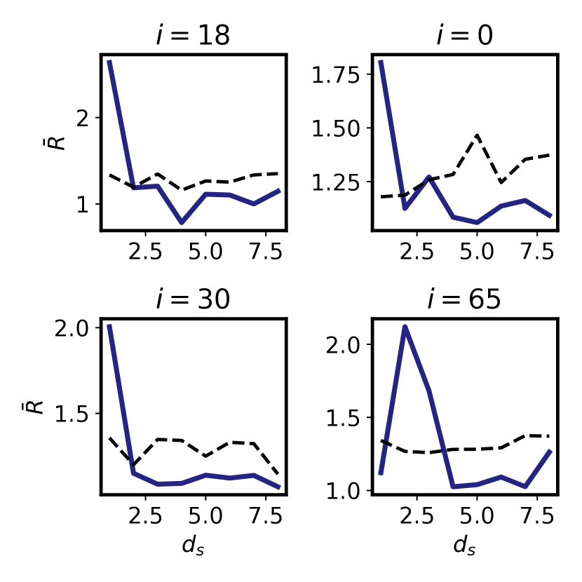
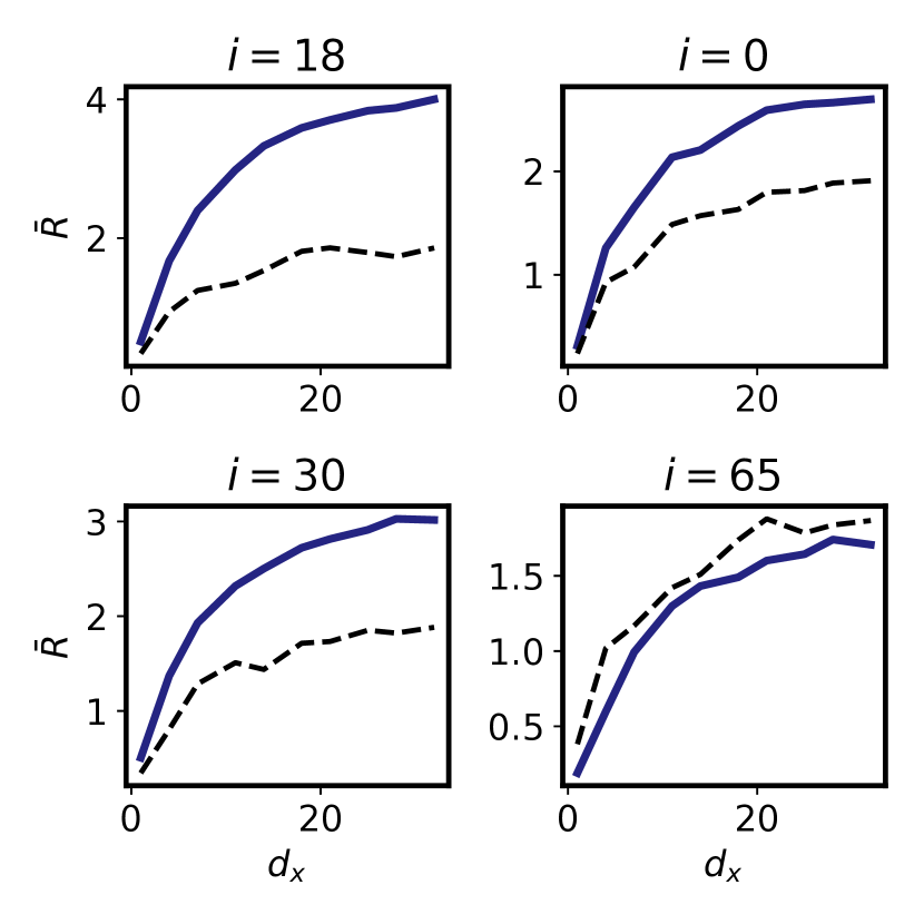
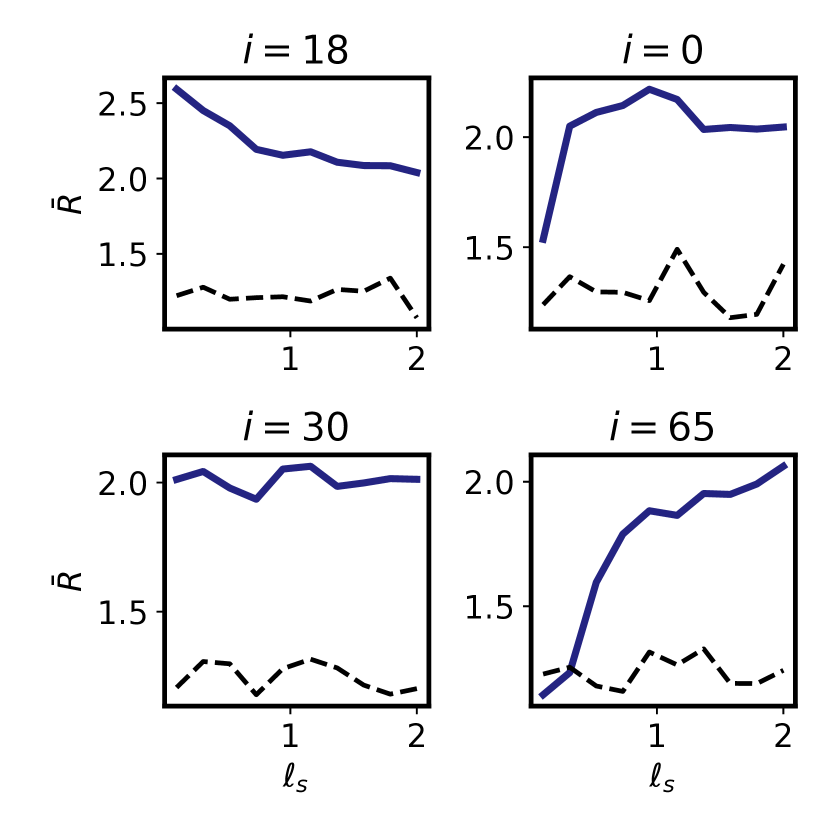
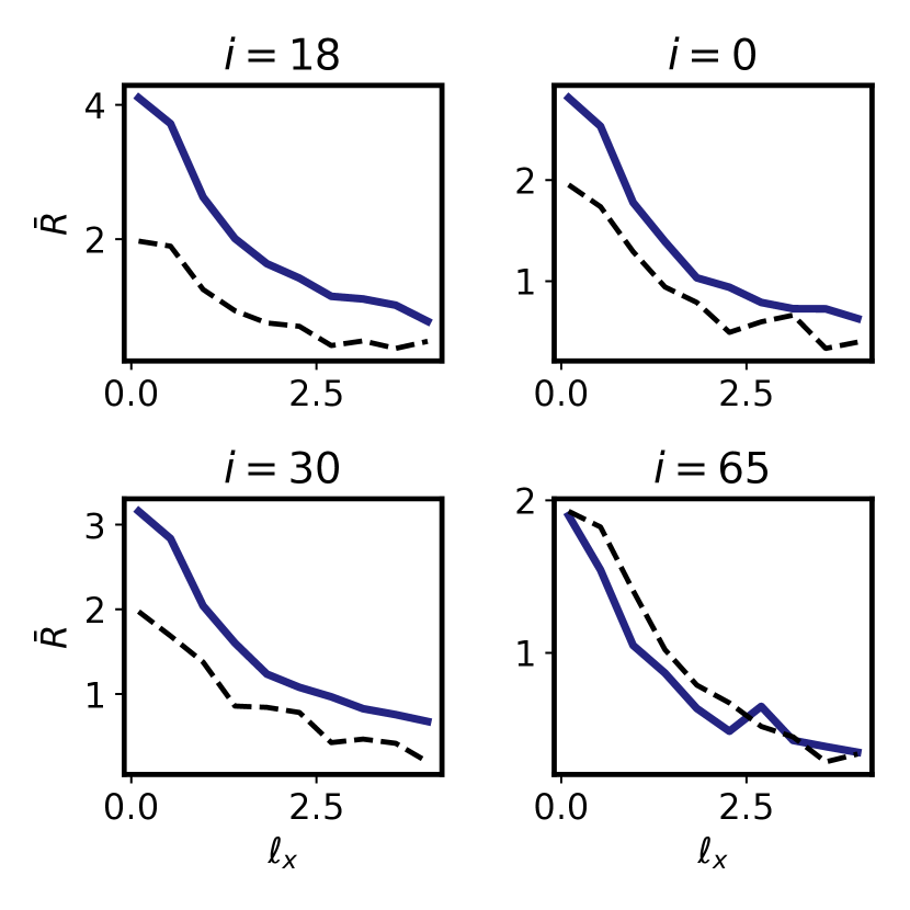
One reason to carry out simulation studies is to assess the sensitivity of the screening procedure on specific parameters. The supplemental information (Section SI.2) provide results for several such simulation results, in which specific parameters were varied. Here we focus on two for illustration.

Figure 1(a) shows the expected reward obtained as a function of the budget $C_{\text{max}}$, which is varied from 1000 to 50,000. We note that a budget of 50,000 is exactly the cost to exhaustively evaluate the $m=500$ candidates once during the final stage, each evaluation incurring a cost $c_{3}=100$. The solid blue lines plot the expected optimal reward under the XPLT meta-policy, while the dashed black line shows the expected rewards under the random policy. The four plots each correspond to four different choices of priors, and hence represent four different problems, each with unique statistical relations between candidates and stages. We note that in general, the performance of both policies increase as the computational budget increases. Yet, depending on the distribution, the marginal returns obtained from increasing the budget varies. For example, in panel C, there is little marginal improvement to the expected reward even as we increase the budget by an order of magnitude. In panel B, we obtain good marginal improvement only up to $C_{\text{max}}=3000$. The bottom-right panel (panel D) shows it is possible for the screening procedure to consistently perform worse than random for some problem settings.

(a) Expected rewards vs. $C_{\text{max}}$

(b) Expected rewards vs. $m$

Figure 1: Expected rewards vs. specific pipeline parameters. Solid blue lines are the expected optimal rewards obtained from the XPLT-based screening procedure, while the dashed black line show the expected rewards obtained under the random (non-screening) policy. Each sub-panel (A, B, C, and D) corresponds to a different prior distribution, and hence a different problem. Specifically, the prior distributions differ with respect to stage-wise similarities, as described in Section 4.2.

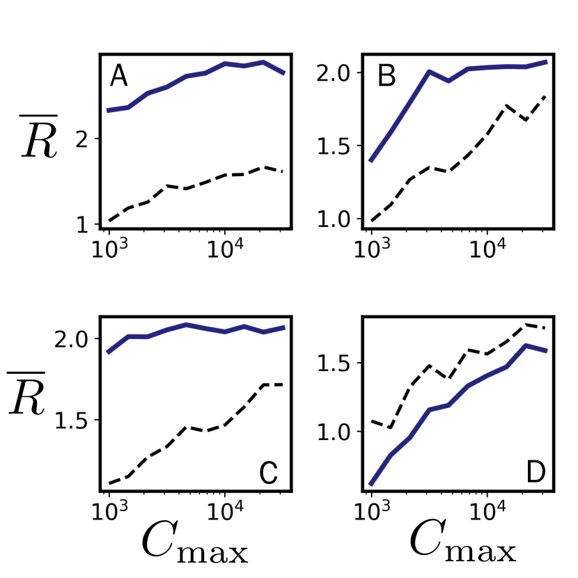
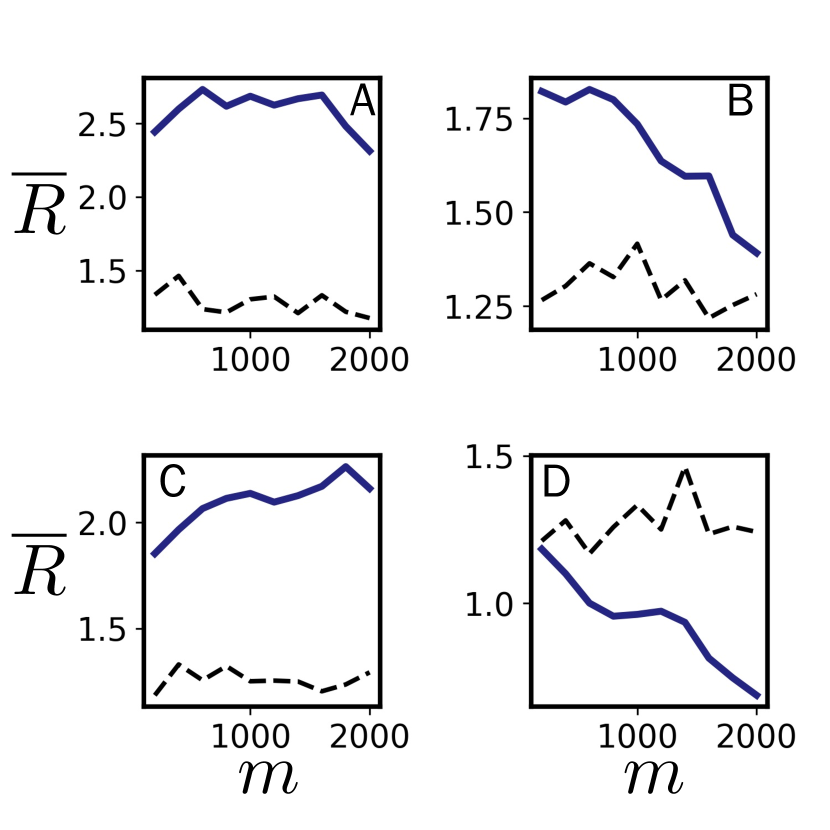
Figure 1(b) shows the expected reward obtained versus the number of initial candidates $m$, varying this number between 500 and 2000. We note that the performance of the random policy is not sensitive to this value. With the fixed budget $C_{\text{max}}=2500$ and a final-stage cost $c_{3}=100$, the random policy can try 25 out of $m$ total candidates. As the simulations suggest, the chance that one of 25 selected candidates yields a large reward is relatively stable (and low) for $m$ between 500 and 2000. In contrast, the expected optimal rewards obtained from the XPLT policy shows varying behavior depending on the prior distribution. In panel A, the expected optimal rewards is relatively insensitive to $m$, while in panel C, these rewards increase with $m$. Panels B and D show the opposite behavior, where the performance decreases with respect to $m$. As with the previous study, we see that the screening procedure performs worse than random in panel D.

It is interesting to note the different trends in expected optimal reward versus different problem parameters or distributions of the ground truth, and how such trends compare to random. The above simulations and those in SI.2 make clear that the analysis is not straight forward and that there is no one general “rule-of-thumb” when it comes to setting these parameters. Therefore, in practice, it is important to assess the problem setting (in the above: which of A, B, C, or D) prior to executing a screening pipeline or even selecting policy parameters using ad hoc or heuristic methods. Simulations offer a systematic way of studying such effects.

Effect of prior distribution

Figure 2: Expected reward distributions over different priors.

As we see above, the trends of expected rewards could depend on the prior distribution, since the real ground truth is sampled from this distribution in these truth-from-prior studies. It is therefore desirable to characterize this dependence further, and see if there are any features of a distribution or problem that predict effectiveness of the screening procedure. The prior distribution is characterized by the latent samples of candidates, $\mathbf{X}=\left\{\mathbf{x}_{i}\right\}_{i=1}^{m}$, of stages $\mathbf{S}=\left\{\mathbf{s}_{j}\right\}_{j=1}^{n}$, and parameters such at the dimensionality of such samples $d_{x}$ and $d_{s}$, and the covariance function hyperparameters $\ell_{x},\ell_{s},\sigma_{x}$ and $\sigma_{s}$. The SI details simulation studies for these parameters. Here, we study the impact of the samples $\mathbf{X}$ and $\mathbf{S}$.

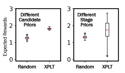
By considering several such latent samples, we obtain distributions of expected rewards, which are shown in Figure 2. The left panel shows the induced distribution on expected reward as we vary the latent samples on candidates $\mathbf{X}$, for both the XPLT policy and the random baseline policy. As we see, the distributions for both policies are insensitive to the specific choice of latent samples, typified by the tight induced distributions. In contrast, the right panel shows these distributions as we vary stage latent samples $\mathbf{S}$. Here, we see that the expected reward is highly sensitive to the actual latent samples of stages, implying that stage-wise covariance structure significantly impacts the overall effectiveness of the screening procedure. We even see that a significant proportion of sampled priors result in the screening procedure performing worse than random.

Figure 3: Similarities between stages dictate expected rewards. This plot shows expected realized rewards for different prior distributions. Locations of the plotted points indicate the distance between first and second stages, and first and third stages. Color indicates the expected realized rewards, while size is inversely proportional to the variance of the realized rewards. Inverted triangles indicate cases where the expected reward obtained via screening was less than that obtained via random sampling.

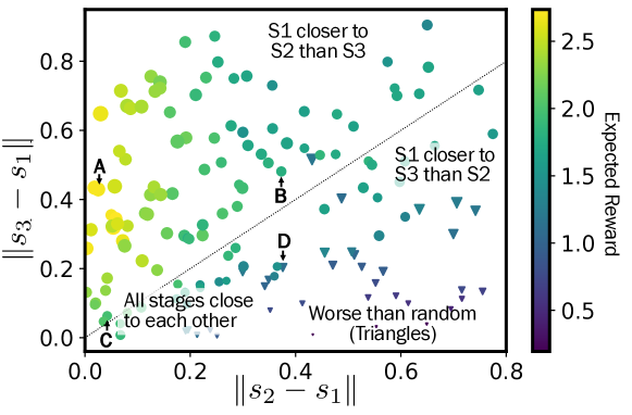
To further explore this phenomenon, we consider the optimal rewards obtained by the XPLT policy for several samples of $\mathbf{S}=(\mathbf{s}_{1},\mathbf{s}_{2},\mathbf{s}_{3})$, and hence for several different priors distributions. We characterize these rewards with respect to two geometric features derived from the latent stage representation: the distance between the latent representations of Stage 1 and Stage 2 $\|\mathbf{s}_{2}-\mathbf{s}_{1}\|$ and the distance between Stage 1 and Stage 3 $\|\mathbf{s}_{3}-\mathbf{s}_{1}\|$. These distances typify the statistical relationship between the stages. This data is displayed in Figure 3.

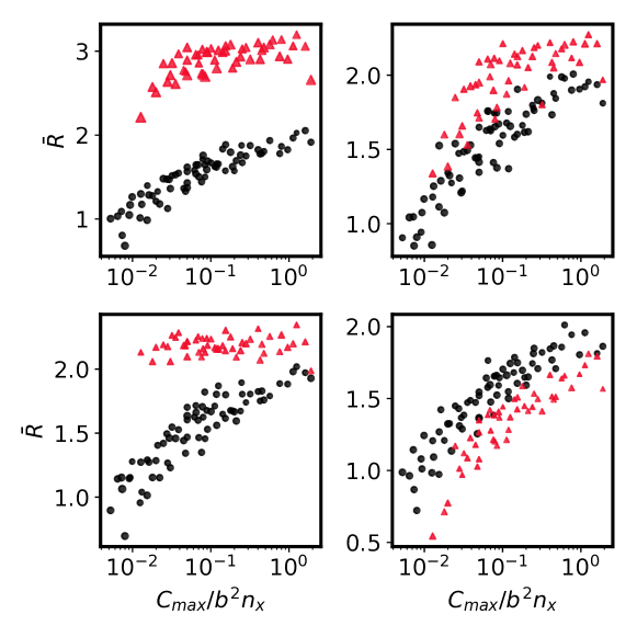
Each dot in the figure corresponds to a specific sample of latent stages i.e. a specific distribution for ground truth. Dots are located at coordinates $(\|\mathbf{s}_{2}-\mathbf{s}_{1}\|,\|\mathbf{s}_{3}-\mathbf{s}_{1}\|)$. For example, points in the lower-left corner correspond to the case where the three stages are statistically similar, while dots in the top-left corner correspond to the case where Stages 1 and 2 are similar, but the Stages 1 and 3 are not. The color of a dot indicates the expected optimal reward given the specific prior distribution corresponding to that dot. The size of the dot is inversely proportional to the variance of the reward distribution. Smaller dots are cases where there is a wide distribution of rewards associated to the selected optimal allocation. Circles indicate the cases where the XPLT policy performs better than random given the same prior distribution, while inverted triangles show the cases where it performs worse than random. The points labeled A, B, C and D correspond to the specific prior distributions used in the single-parameter simulation studies in Section 4.1 above and in the SI.

The dashed line indicates the points where Stage 3 and Stage 2 are both equidistant to Stage 1. Points above this line refer to cases where Stage 1 is more statistically similar to Stage 2 than to Stage 3. Points below this line correspond to cases where Stage 1 is more similar to Stage 3 than to Stage 2. In this region, the statistical similarities between stages do not respect the order in which the stages are executed in the pipeline. From the plot, the screening procedure is not effective in this region, often performing worse than random. There is a general improvement as Stage 2 and Stage 1 become more similar, i.e. as we move right to left along the horizontal axis. Interestingly, this trend does not hold with respect to Stage 3. From the plot, there appears to be an optimal dissimilarity between Stages 1 and 3 that yield maximal expected rewards. For example, among the samples, Point A corresponds to the largest expected reward. For this point the distance between $\mathbf{s}_{3}$ and $\mathbf{s}_{1}$ is around 0.42.

This optimal dissimilarity for this model system again indicates the need to perform such simulations for real systems in practice. In this specific case, tuning similarity between stages to match the optimal settings identified through such simulation studies could mean tuning the accuracy of a ML model, increasing or decreasing simulation run times or resolutions, or introducing randomness (i.e. exploration) in selecting candidates to advance between stages. Having a proper assessment of the impact of such pipeline parameters could then result in more efficient and effective screening.

Throughput and optimal reward

Figure 4: Throughput correlates with expected optimal reward. This figure plots expected optimal reward versus final-stage allocation $m^{\star}_{3}$ of the optimal allocation $\mathbf{m}^{\star}$ selected by the XPLT policy. Each dot corresponds to a different prior distribution. The size of each dot is inversely proportional to the variance of the reward distribution $r(\mathbf{m}^{\star})$.

Another pipeline study [26] examined the pipeline problem under different design variables and objectives. There, authors considered score thresholds (rather than explicit allocations) as the design variables. They also considered the objective of optimizing pipeline throughput – the number of candidates that satisfy all thresholds to make it past the final stage, under similar cost constraints as those detailed above. In this setting, the pipeline is used to maximize the number of good candidates passing through the screening procedure. While not the same problem as considered here, we are nevertheless able to draw some connections between our work and this optimal throughput problem.

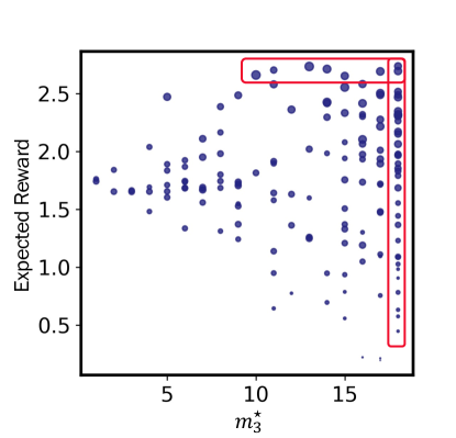
Figure 4 plots the expected optimal reward $\overline{R}(\mathbf{m}^{\star})$ versus the final stage allocation $m^{\star}_{3}$, for different sampled prior distributions. Each dot corresponds to the expected optimal reward and final stage allocation obtained for a specific prior distribution. As before, the size of the dot is inversely proportional to the variance of the reward distribution. The red rectangles call attention to settings with high expected rewards (top), and those that have large final allocation (right). The final allocation is the measure for throughput. While in our study we optimized for expected rewards rather than throughput, we observe from the plot that the two quantities are correlated

Namely, we note that for the settings resulting in the highest expected reward (top box), the final stage allocation $m^{\star}_{3}$ was around 10 or larger. Given the final stage cost $c_{3}=100$ and budget $C_{\text{max}}=2500$, this means that optimal allocations yielding highest expected rewards were expending around 40 to 60% of the budget on final stage trials. We note that for cases where the optimal final allocation is large (right box), there is a spread of both high and low expected rewards. Yet, the concentration is biased toward the high expected reward regime. Moreover the high-throughput / low expected reward cases are associated with large variance of reward distribution. These results show that while the relationship between throughput and expected rewards may be complex, there are broad agreements between the two optimization objectives, though there are cases where this agreement may not hold.

Conclusion

In this paper, we defined a model and algorithm for simulating pipelines, and identified places where such methods can be used to perform decision-making under uncertainty via simulation-based policies. We codified how various different pipeline objectives fit inside the common framework of optimizing expected rewards under uncertainty, and alluded to a multi-faceted, rich problem set that belies the ubiquitous experimental protocol of multi-stage screening.

Examining one part of this problem landscape, we focused on analyzing a popular mode for screening: simply selecting the top $m_{j}$ candidates from the previous stage to pass onto the next stage. We showed how to optimize expected rewards with respect to a specific design parameter choice, allocation, in a one-shot setting. In this specific context, our simulation studies showed a variety of trends as we attempted to characterize the effectiveness of the screening procedure with respect to pipeline or problem parameters. We most importantly described how stage-wise covariance structure played a significant role in determining this efficacy. We demonstrated how simulated studies allowed us to quantify the performance, its dependence on parameters, and in comparison with a random baseline policy.

We hope to have demonstrated the need for proper modeling and analysis in multi-stage screening pipeline optimization, decision-making and parameter calibration. We believe that the models, policies and simulation methods presented in this paper provide important tools in this analysis.

Conflict of interest statement

On behalf of all authors, the corresponding author states that there is no conflict of interest.

Appendix SI.1 Iterative algorithm for lazy stage-wise sampling

In this section, we introduce the equations to express the parameters of the relevant marginal and conditional normal distributions used to perform lazy stage-wise sampling of scores, under separable covariance assumption. As before, we shall let $n$ be the number of stages, and $m$ be the number of initial candidates. Let

$$\mathbf{Y}=\begin{pmatrix}\mathbf{Y}_{1}\\ \mathbf{Y}_{2}\\ \vdots\\ \mathbf{Y}_{n}\end{pmatrix}$$

be the $nm$-dimensional vector of scores, expressed in block form so that $\mathbf{Y}_{j}\in\mathbb{R}^{m}$ represents the $m$ scores for all candidates at stage $j$. Concatenating all but the first block, we may write

$$\mathbf{Y}=\begin{pmatrix}\mathbf{Y}_{1}\\ \mathbf{Y}_{2:}\end{pmatrix},$$

with the concatenation is denoted as $\mathbf{Y}_{2:}=(\mathbf{Y}_{2},\ldots,\mathbf{Y}_{n})^{T}$.

Suppose $\mathbf{Y}\sim\mathcal{N}(\bm{\mu},\Gamma)$ is multivariate normal distributed, with the mean vector $\bm{\mu}\in\mathbb{R}^{nm}$ and covariance matrix $\Gamma\in\mathbb{R}^{nm\times nm}$ given in block form as:

$$\bm{\mu}=\begin{pmatrix}\bm{\mu}_{1}\\ \bm{\mu}_{2:}\end{pmatrix},\quad\quad\Gamma=\begin{pmatrix}\Gamma_{1,1}&\Gamma_{1,2:}\\ \Gamma_{2:,1}&\Gamma_{2:,2:}\end{pmatrix}.$$

Here, $\Gamma_{1,1}$ is the $m\times m$ covariance matrix between all candidates for the first stage, while $\Gamma_{1,2:}=\Gamma_{2:,1}^{T}$ is the $m\times(nm-m)$ matrix of cross-covariances between the scores of all candidates at the first stage, and at later stages. $\Gamma_{2:,2:}$ is the $(nm-m)\times(nm-m)$ covariance matrix for the scores of all candidates at all other stages except for the first. As before, we view $\Gamma$ as separable and write $\Gamma=\Sigma\otimes X$. We can similarly write the stage covariance matrix $\Sigma$ in block-form as:

$$\Sigma=\begin{pmatrix}\Sigma_{1,1}&\Sigma_{1,2:}\\ \Sigma_{2:,1}&\Sigma_{2:,2:}\end{pmatrix},$$

so that $\Sigma_{1,1}$ is a scalar, $\Sigma_{2:,1}=\Sigma_{1,2:}^{T}$ is an $(n-1)\times 1$ vector and $\Sigma_{2:,2:}$ is the $(n-1)\times(n-1)$ sub-covariance matrix for stages 2 through $n$. It follows that $\Gamma_{1,1}=\Sigma_{1,1}\otimes X$, $\Gamma_{2:,1}=\Sigma_{2:,1}\otimes X$ and $\Gamma_{2:,2:}=\Sigma_{2:,2:}\otimes X$

We may obtain a sample of just the first stage scores $\mathbf{Y}_{1}$ by noticing the marginal distribution is also normal. That is $\mathbf{Y}_{1}\sim\mathcal{(}\bm{\mu}_{1},\Gamma_{1,1})$. Suppose $X$ admits a Cholesky factorization $X=LL^{T}$. Then $\Gamma_{1,1}$ admits a Cholesky factorization $\Gamma_{1,1}=(\sqrt{\Sigma_{1,1}}L)(\sqrt{\Sigma_{1,1}}L)^{T}$. We can use this to sample first-stage scores:

$$\mathbf{y}_{1}=\bm{\mu}_{1}+\sqrt{\Sigma_{1,1}}L\mathbf{z},$$

where $\mathbf{z}\sim\mathcal{N}(0,I_{m})$ is a sample of $m$ independent, standard normal random variables.

Once the first stage scores are sampled, we can update the distribution of scores for later stages, conditional on the sampled scores. This conditional distribution is also normal, namely $\mathbf{Y}_{2:}|\mathbf{Y}_{1}=\mathbf{y}_{1}\sim\mathcal{N}\left(\bm{\mu}_{2:}^{\prime},\Gamma^{\prime}_{2:,2:}\right),$ where

$$\bm{\mu}_{2:}^{\prime} =\bm{\mu}_{2:}+\Gamma_{2:,1}\Gamma_{1,1}^{-1}(\mathbf{y}_{1}-\bm{\mu}_{1}),$$

$$=\bm{\mu}_{2:}+(\Sigma_{2:,1}\otimes L)(\Sigma_{1,1}\otimes L)^{-1}(\mathbf{y}_{1}-\bm{\mu}_{1}),$$

$$=\bm{\mu}_{2:}+\frac{1}{\Sigma_{1,1}}\left(\Sigma_{2:,1}\otimes(\mathbf{y}_{1}-\bm{\mu}_{1})\right),$$

$$\Gamma_{2:,2:}^{\prime} =\Gamma_{2:,2:}-\Gamma_{2:,1}\Gamma_{1,1}^{-1}\Gamma_{1,2:}.$$

$$=\left(\Sigma_{2:,2:}-\Sigma_{2:,1}\Sigma_{1,1}^{-1}\Sigma_{1,2:}\right)\otimes X,$$

$$=\left(\Sigma_{2:,2:}-\frac{\Sigma_{2:,1}\Sigma_{2:,1}^{T}}{\Sigma_{1,1}}\right)\otimes X,$$

$$=\tilde{\Sigma}\otimes X,$$

Here, $\tilde{\Sigma}=\Sigma_{2:,2:}-\Sigma_{2:,1}\Sigma_{2:,1}^{T}/\Sigma_{1,1}$

In addition to sampling scores for the first stage, and updated the distribution for later stages, the inter-stage policy will choose some candidates that will not pass through to the second stage, and hence we do not need to sample scores for these entries at later stages. Namely, we shall filter out $\Delta m=m_{2}-m_{1}$ candidates. Let $\tilde{L}$ be the $m_{2}\times m$ matrix resulting from removing the appropriate $\Delta m$ rows of $L$ and let $\tilde{\bm{\mu}}$ be the $m_{2}\cdot(n-1)$-length vector resulting from removing the appropriate $(n-1)\cdot\Delta m$ rows from $\bm{\mu}_{2:}$ corresponding to the filtered candidates for each of the remaining $n-1$ stages.

At the end of this procedure, we have the updated conditional distribution:

$$\tilde{\mathbf{Y}} \sim\mathcal{N}(\tilde{\bm{\mu}},\tilde{\Gamma}),$$

$$\tilde{\Gamma} =\tilde{\Sigma}\otimes\tilde{X},$$

$$\tilde{X} =\tilde{L}\tilde{L}^{T}.$$

which describes the score distribution for the remaining $m_{2}$ candidates, for the remaining $n-1$ stages. The procedure above can be repeated to sample scores for the second stage and update the distribution for the third, and so on. As we see above, the sampling and conditioning operations depend on our ability to maintain and update the mean score vector $\bm{\mu}$, the stage covariance matrix $\Sigma$ and the Cholesky factor of the candidate covariance matrix $L$ as we simulate the pipeline. At stage $j$ of the pipeline, these updated matrices are of size $m_{j}\cdot n$, $(n-j+1)\times(n-j+1)$ and $m_{j}\times m$, respectively, a dramatic departure from the $(nm)\times(nm)$ scaling required for naïve sampling.

Appendix SI.2 Further simulation studies

(a) $d_{s}$

(b) $d_{x}$

(c) $\ell_{s}$

(d) $\ell_{x}$

Figure 5: Single parameter simulation studies for covariance prior parameters. The order of the panels correspond to points A, B, C, and D as in the main text.

Figure 6: We parameterize cost as $\mathbf{c}=(b^{0},b^{1},b^{2})$. The quantity $C_{\text{max}}/b^{2}m$ is the proportion between the given budget $C_{\text{max}}$ and the cost to exhaustively try all candidates $b^{2}m$. We plot this versus expected rewards for various choices of $C_{\text{max}},b$ and $m$.

References

- [1] A. D. Andricopulo, R. V. Guido, and G. Oliva, “Virtual screening and its integration with modern drug design technologies,” Current medicinal chemistry, vol. 15, no. 1, pp. 37–46, 2008.
- [2] G. Schneider and H.-J. Böhm, “Virtual screening and fast automated docking methods,” Drug Discovery Today, vol. 7, pp. 64–70, 2002.
- [3] M. Kandeel and M. Al-Nazawi, “Virtual screening and repurposing of fda approved drugs against covid-19 main protease,” Life sciences, vol. 251, p. 117627, 2020.
- [4] J. Bajorath, “Integration of virtual and high-throughput screening,” Nature Reviews Drug Discovery, vol. 1, no. 11, pp. 882–894, 2002.
- [5] B. K. Shoichet, “Virtual screening of chemical libraries,” Nature, vol. 432, no. 7019, pp. 862–865, 2004.
- [6] R. Gómez-Bombarelli, J. Aguilera-Iparraguirre, T. D. Hirzel, D. Duvenaud, D. Maclaurin, M. A. Blood-Forsythe, H. S. Chae, M. Einzinger, D.-G. Ha, T. Wu, et al., “Design of efficient molecular organic light-emitting diodes by a high-throughput virtual screening and experimental approach,” Nature materials, vol. 15, no. 10, pp. 1120–1127, 2016.
- [7] E. O. Pyzer-Knapp, C. Suh, R. Gómez-Bombarelli, J. Aguilera-Iparraguirre, and A. Aspuru-Guzik, “What is high-throughput virtual screening? a perspective from organic materials discovery,” Annual Review of Materials Research, vol. 45, pp. 195–216, 2015.
- [8] E. O. Pyzer-Knapp, G. N. Simm, and A. A. Guzik, “A bayesian approach to calibrating high-throughput virtual screening results and application to organic photovoltaic materials,” Materials Horizons, vol. 3, no. 3, pp. 226–233, 2016.
- [9] K. Abdel-Latif, R. W. Epps, F. Bateni, S. Han, K. G. Reyes, and M. Abolhasani, “Self-driven multistep quantum dot synthesis enabled by autonomous robotic experimentation in flow,” Advanced Intelligent Systems, vol. 3, no. 2, p. 2000245, 2021.
- [10] A. E. Gongora, K. L. Snapp, E. Whiting, P. Riley, K. G. Reyes, E. F. Morgan, and K. A. Brown, “Using simulation to accelerate autonomous experimentation: A case study using mechanics,” Iscience, vol. 24, no. 4, p. 102262, 2021.
- [11] S. Baek and K. G. Reyes, “Problem-fluent models for complex decision-making in autonomous materials research,” Computational Materials Science, vol. 193, p. 110385, 2021.
- [12] A. Tropsha and A. Golbraikh, “Predictive qsar modeling workflow, model applicability domains, and virtual screening,” Current pharmaceutical design, vol. 13, no. 34, pp. 3494–3504, 2007.
- [13] C.-A. Azencott, A. Ksikes, S. J. Swamidass, J. H. Chen, L. Ralaivola, and P. Baldi, “One-to four-dimensional kernels for virtual screening and the prediction of physical, chemical, and biological properties,” Journal of chemical information and modeling, vol. 47, no. 3, pp. 965–974, 2007.
- [14] Q. U. Ain, A. Aleksandrova, F. D. Roessler, and P. J. Ballester, “Machine-learning scoring functions to improve structure-based binding affinity prediction and virtual screening,” Wiley Interdisciplinary Reviews: Computational Molecular Science, vol. 5, no. 6, pp. 405–424, 2015.
- [15] P. J. Ballester and J. B. Mitchell, “A machine learning approach to predicting protein–ligand binding affinity with applications to molecular docking,” Bioinformatics, vol. 26, no. 9, pp. 1169–1175, 2010.
- [16] B. Sanchez-Lengeling and A. Aspuru-Guzik, “Inverse molecular design using machine learning: Generative models for matter engineering,” Science, vol. 361, no. 6400, pp. 360–365, 2018.
- [17] J. Lim, S. Ryu, J. W. Kim, and W. Y. Kim, “Molecular generative model based on conditional variational autoencoder for de novo molecular design,” Journal of cheminformatics, vol. 10, no. 1, pp. 1–9, 2018.
- [18] W. Gao and C. W. Coley, “The synthesizability of molecules proposed by generative models,” Journal of chemical information and modeling, vol. 60, no. 12, pp. 5714–5723, 2020.
- [19] K. Deb, “Multi-objective optimization,” in Search methodologies, pp. 403–449, Springer, 2014.
- [20] N. Beume, B. Naujoks, and M. Emmerich, “SMS-EMOA: Multiobjective selection based on dominated hypervolume,” European Journal of Operational Research, vol. 181, no. 3, pp. 1653–1669, 2007.
- [21] Y. Wang, K. G. Reyes, K. A. Brown, C. A. Mirkin, and W. B. Powell, “Nested-batch-mode learning and stochastic optimization with an application to sequential multistage testing in materials science,” SIAM Journal on Scientific Computing, vol. 37, no. 3, pp. B361–B381, 2015.
- [22] J. Snoek, H. Larochelle, and R. P. Adams, “Practical Bayesian optimization of machine learning algorithms,” Advances in neural information processing systems, vol. 25, 2012.
- [23] P. Auer, N. Cesa-Bianchi, and P. Fischer, “Finite-time analysis of the multiarmed bandit problem,” Machine learning, vol. 47, no. 2, pp. 235–256, 2002.
- [24] E. V. Bonilla, K. Chai, and C. Williams, “Multi-task gaussian process prediction,” Advances in neural information processing systems, vol. 20, 2007.
- [25] A. Gelman, J. B. Carlin, H. S. Stern, and D. B. Rubin, Bayesian data analysis. Chapman and Hall/CRC, 1995.
- [26] H.-M. Woo, X. Qian, L. Tan, S. Jha, F. J. Alexander, E. R. Dougherty, and B.-J. Yoon, “Optimal decision making in high-throughput virtual screening pipelines,” arXiv preprint arXiv:2109.11683, 2021.