Anisotropic nature of space-time in $f\left(Q\right)$ gravity

Abstract

In this paper, we consider the Bianchi type-I space-time with perfect fluid as matter content of the Universe in the framework of $f(Q)$ gravity (where $Q$ is the non-metricity scalar) recently proposed by Jiménez et al. (Phys. Rev. D 98.4 (2018): 044048). We find exact solutions of the field equations using the anisotropic property of space-time for volumetric hybrid expansion. The cosmological parameters for the linear form of non-metricity scalar i.e. $f\left(Q\right)=\alpha Q+\beta$ (where $\alpha$ and $\beta$ are free model parameters) are discussed and compared with recent Hubble measurements. Also, we have obtained the best fitting values of the model parameters $k,n$ and $H_{0}$ by constraining our model with updated Hubble datasets consisting of 57 data points ($31$ (DA) and $26$ (BAO+other)) along with also examined the stability of the model and test its validity by energy conditions.

Keywords: Bianchi type-I space-time, $f(Q)$ gravity, Dark energy, Energy conditions.

I Introducion

The theory of general relativity (GR) is the most famous theory of gravity published by Albert Einstein in 1915 [1], for having been experimentally tested more than once, and all the results are surprisingly consistent with the theory’s predictions [2, 3, 4]. According to this theory, gravity is just a curvature of space-time due to the presence of a large mass, and therefore, this theory linked the matter content of the Universe with the geometry of the fabric of the space-time. The geometry of space-time is represented by the Einstein tensor $G_{\mu\nu}$, and matter is represented by the energy-momentum tensor $T_{\mu\nu}$, and thus we get the Einstein field equations as $G_{\mu\nu}=kT_{\mu\nu}$ (in natural units $k=8\pi Gc^{-4}=1$). These equations can be derived by means of a mathematical object called Einstein-Hilbert (EH) action which is given as follows

$$S_{EH}=\int\left[\frac{1}{2}R+\mathcal{L}_{m}\right]d^{4}x\sqrt{-g},$$ (1)

where $g=\det\left(g_{\mu\nu}\right)$ is the determinant of the metric tensor $g_{\mu\nu}$, $R$ is the Ricci scalar and $\mathcal{L}_{m}$ is the matter Lagrangian density. GR is based on an important property that the covariant derivative $\nabla_{\gamma}$ of the metric is zero $\left(\nabla_{\gamma}g_{\mu\nu}=0\right)$ [5]. Despite all the success of this theory, there are major common questions, both theoretical and experimental, for which GR has not found an explanation, such as the initial singularity, dark matter, dark energy (DE), etc. In this paper, we will discuss the DE problem. The DE is an exotic form of energy with negative pressure or negative equation of state (EoS) parameter, because $\omega=\frac{p}{\rho}$, where $\rho$ represents the energy density of the Universe and $p$ represents pressure, and it behaves like a repulsive gravity. The presence of DE in the Universe is supported by two of most important modern cosmological observational facts. The first is the composition of our Universe, this shows that dark energy contributes $68.3\%$ of the total energy density (the rest is dark matter and baryonic matter) [6]. The second is strong evidence coming mainly from type-Ia supernovae (SN-Ia) observations that the Universe is today undergoing an accelerated expansion phase [7, 8]. In order to obtain the accelerating expansion, the second derivative of the scale factor must be positive (i.e. $\overset{..}{a}>0$) or in an equivalent way the deceleration parameter is negative ( i.e. $q=-\frac{a\overset{..}{a}}{\overset{.}{a}^{2}}<0$). The simplest candidate for DE is the cosmological constant $\Lambda$, which is regarded to be equivalent with the vacuum energy. But soon other problems appeared, such as the coincidence and magnitude [9]. Therefore, many researchers have searched for other interpretations about the origin of DE. In fact, two distinct approaches have been proposed for treating the DE problem. The first approach deals with GR where an additional energy component is introduced to explain the cosmic acceleration phenomenon. In this context, several alternative DE models have been suggested, but so far no suitable candidate has been found. The other approach is to modify the EH action. In this context, the main idea was to replace the Ricci scalar by a function of $R$, which is known as $f\left(R\right)$ gravity [10, 11]. Other modified theories have been proposed like $f\left(T\right)$ gravity (where $T$ is the torsion), $f\left(G\right)$ gravity (where $G$ is the Gauss-Bonnet), see these works in this regard [12, 13, 14].

Recently, Jiménez et al. [15] proposed a new modified theory of gravity called $f\left(Q\right)$ gravity where $Q$ is the non-metricity scalar which attracted the attention of many researchers. This theory is based on Weyl geometry, which is a generalization of Riemannian geometry that is the mathematical basis of GR. In Weyl geometry, gravitational effects do not occur because of the change in direction of a vector in parallel transport, but because of the change in length of the vector itself [16]. Generally, we can categorize gravitational interactions in the space-time variety into three types of geometrical objects, specifically the curvature, torsion, and non-metricity. In GR, gravitational interactions are caused by the curvature of space-time. Accordingly, $f\left(R\right)$ gravity is a modification of GR based on curvature with zero torsion and non-metricity. Likewise, $f\left(T\right)$ gravity is a modification of torsion-based gravity (the teleparallel equivalent of GR) with zero curvature and non-metricity. Finally, $f\left(Q\right)$ gravity is a modification of the symmetric teleparallel equivalent of GR with zero curvature and torsion [17, 18]. In differential geometry and to be more precise in Weyl-Cartan geometry, we need the symmetric metric tensor $g_{\mu\nu}$ to define the length of a vector, and an asymmetric connection $\widetilde{{\Gamma}}{{}^{\gamma}}_{\mu\nu}$ in order to defines the covariant derivatives and parallel transport. Thus, the general affine connection can be decomposed into three parts: the Christoffel symbol ${\Gamma^{\gamma}}_{\mu\nu}$, the contortion tensor ${C^{\gamma}}_{\mu\nu}$, and the disformation tensor ${L^{\gamma}}_{\mu\nu}$, respectively, which are written as [16]

$$\widetilde{{\Gamma}}{{}^{\gamma}}_{\mu\nu}={\Gamma^{\gamma}}_{\mu\nu}+{C^{\gamma}}_{\mu\nu}+{L^{\gamma}}_{\mu\nu},$$ (2)

where the Levi-Civita connection of the metric $g_{\mu\nu}$ is given by

$${\Gamma^{\gamma}}_{\mu\nu}\equiv\frac{1}{2}g^{\gamma\sigma}\left(\frac{\partial g_{\sigma\nu}}{\partial x^{\mu}}+\frac{\partial g_{\sigma\mu}}{\partial x^{\nu}}-\frac{\partial g_{\mu\nu}}{\partial x^{\sigma}}\right),$$ (3)

the contorsion tensor ${C^{\gamma}}_{\mu\nu}$ is

$${C^{\gamma}}_{\mu\nu}\equiv\frac{1}{2}{T^{\gamma}}_{\mu\nu}+T_{(\mu}{}^{\gamma}{}_{\nu)},$$ (4)

with ${T^{\gamma}}_{\mu\nu}\equiv 2{\Gamma^{\gamma}}_{[\mu\nu]}$ in the above equation is the torsion tensor. Lastly, the disformation tensor ${L^{\gamma}}_{\mu\nu}$ is obtained from the non-metricity tensor as

$${L^{\gamma}}_{\mu\nu}\equiv\frac{1}{2}g^{\gamma\sigma}\left(Q_{\nu\mu\sigma}+Q_{\mu\nu\sigma}-Q_{\gamma\mu\nu}\right).$$ (5)

In Eq. (5), the non-metricity tensor $Q_{\gamma\mu\nu}$ is defined as the (minus) covariant derivative of the metric tensor with regard to the Weyl-Cartan connection $\widetilde{\Gamma}_{\mu\nu}^{\lambda}$, i.e. $Q_{\gamma\mu\nu}=\nabla_{\gamma}g_{\mu\nu}$, and it can be gained

$$Q_{\gamma\mu\nu}=-\frac{\partial g_{\mu\nu}}{\partial x^{\gamma}}+g_{\nu\sigma}\widetilde{{\Gamma}}{{}^{\sigma}}_{\mu\gamma}+g_{\sigma\mu}\widetilde{{\Gamma}}{{}^{\sigma}}_{\nu\gamma}.$$ (6)

In the case of a flat and torsion-free connection, the connection (2) can be parameterized as

$$\widetilde{{\Gamma}}{{}^{\gamma}}_{\mu\beta}=\frac{\partial x^{\gamma}}{\partial\xi^{\rho}}\partial_{\mu}\partial_{\beta}\xi^{\rho}.$$ (7)

In Eq. (7), $\xi^{\gamma}=$ $\xi^{\gamma}\left(x^{\mu}\right)$ is an invertible relation. Therefore, it is constantly potential to get a coordinate system so that the connection $\widetilde{\Gamma}_{\mu\nu}^{\gamma}$ disappears. This condition is called coincident gauge and the covariant $\nabla_{\gamma}$ derivative reduces to the partial derivative $\partial_{\gamma}$ [18]. Hence, in the coincident gauge coordinate, we get

$$Q_{\gamma\mu\nu}=\partial_{\gamma}g_{\mu\nu}.$$ (8)

The symmetric teleparallel gravity is a geometric description of gravity equivalent to GR under coincident gauge coordinates in which $\widetilde{{\Gamma}}{{}^{\gamma}}_{\mu\nu}=0$ and ${C^{\gamma}}_{\mu\nu}=0$, and therefore from Eq. (2) we can conclude that ${\Gamma^{\gamma}}_{\mu\nu}=-{L^{\gamma}}_{\mu\nu}$ [16]. This theory has received great interest from many authors because it gives good results for several issues. The first cosmological solutions in $f(Q)$ gravity emerge in Ref. [19]. Next, Mandal et al. presented a complete test of energy conditions for $f\left(Q\right)$ gravity models and constraint families of $f\left(Q\right)$ models compatible with the current accelerating expansion of the Universe [20]. The cosmography in $f\left(Q\right)$ gravity is also discussed by Mandal et al. in another work [21]. The growth index of matter perturbations has been examined in the context of $f\left(Q\right)$ gravity in [22]. The geodesic deviation equation in $f\left(Q\right)$ gravity has been explored and some fundamental results were gained in [23]. Harko et al. discussed the coupling matter in modified $f(Q)$ gravity [24]. Dimakis et al. investigated quantum cosmology for a $f\left(Q\right)$ polynomial model [25]. Holographic dark energy models in $f\left(Q\right)$ gravity are discussed by Shekh [26]. To study the early evolution of the Universe, A. De et al. obtained the Bianchi-I-type field equations in $f\left(Q\right)$ gravity and some cosmological parameters are discussed in this context [27] and, several other issues in $f\left(Q\right)$ gravity are discussed in Refs. [28, 29, 30, 31]. Motivated from the studies outlined above, in this paper, we have investigated the perfect fluid solutions for Bianchi type-I space-time in $f\left(Q\right)$ gravity. Also, the modified Friedmann equations are obtained by applying the anisotropic nature of space-time. Finally, we have discussed some of the physical parameters of the model and have compared with recent Hubble measurements.

The current article is organized as follows: In Sec. II, we present the basic formalism of $f\left(Q\right)$ gravity and field equations of the Bianchi type-I space-time. We establish the solutions of the anisotropic cosmological model with the choice of a linear $f\left(Q\right)$ function i.e. $f\left(Q\right)=\alpha Q+\beta$, and examined some physical parameters in Sec. III. In Sec. IV, we consider the stability analysis of the anisotropic model by means of the squared sound speed, and we test the validity of the model using energy conditions. We give some physical parameters in terms of redshift in Sec. V. Finally, we discuss the best fit values of model parameters from observation in Sec. VII and in sec. LABEL:sec7 we presents the conclusion and discussion.

II Field equations in $f\left(Q\right)$ gravity

In modified symmetric teleparallel gravity or $f\left(Q\right)$ gravity, the action is given by [19]

$$S=\int\left[\frac{1}{2}f(Q)+\mathcal{L}_{m}\right]d^{4}x\sqrt{-g},$$ (9)

where $f(Q)$ is an arbitrary function of the non-metricity scalar $Q$. The non-metricity tensor and its traces are obtained as

$$Q_{\gamma\mu\nu}=\nabla_{\gamma}g_{\mu\nu}\,,$$ (10)

$$Q_{\gamma}={{Q_{\gamma}}^{\mu}}_{\mu}\,,\qquad\widetilde{Q}_{\gamma}={Q^{\mu}}_{\gamma\mu}\,.$$ (11)

Moreover, the superpotential tensor (non-metricity conjugate) is given by

$$4{P^{\gamma}}_{\mu\nu}=-{Q^{\gamma}}_{\mu\nu}+2Q_{({\mu^{{}^{\gamma}}}{\nu})}-Q^{\gamma}g_{\mu\nu}-\widetilde{Q}^{\gamma}g_{\mu\nu}-\delta_{{(\gamma^{{}^{Q}}}\nu)}^{\gamma}\,,$$ (12)

Next, the trace of the non-metricity tensor can be obtained as

$$Q=-Q_{\gamma\mu\nu}P^{\gamma\mu\nu}\,.$$ (13)

Furthermore, the matter energy-momentum tensor is of the form

$$T_{\mu\nu}=-\frac{2}{\sqrt{-g}}\frac{\delta(\sqrt{-g}\mathcal{L}_{m})}{\delta g^{\mu\nu}}\,.$$ (14)

The field equations in symmetric teleparallel gravity corresponding to action (9) are

$$\frac{2}{\sqrt{-g}}\nabla_{\gamma}\left(\sqrt{-g}f_{Q}P^{\gamma}{}_{\mu\nu}\right)+\frac{1}{2}fg_{\mu\nu}+f_{Q}\left(P_{\mu\gamma i}Q_{\nu}{}^{\gamma i}-2Q_{\gamma i\mu}P^{\gamma i}{}_{\nu}\right)=-T_{\mu\nu},$$ (15)

where the subscript marks the derivative with respect to $Q$. In addition, we can also take the variation of (9) with respect to the connection, which gives

$$\nabla_{\mu}\nabla_{\gamma}\left(\sqrt{-g}f_{Q}P^{\gamma}{}_{\mu\nu}\right)=0.$$ (16)

We consider the matter content of the Universe as a perfect fluid which energy-momentum tensor is

$$T_{\mu\nu}=\left(\rho+p\right)u_{\mu}u_{\nu}+pg_{\mu\nu},$$ (17)

where $\rho$ and$\ p$ are the energy density and pressure of the matter content. The four-velocity vector $u^{\mu}$ is presumed to satisfy $u^{\mu}u_{\mu}=-1$.

The Bianchi type-I space-time is a single of the simplest form of anisotropic space-time, which represents a homogeneous and spatially flat space-time. Hence, In this paper, we consider Bianchi type-I space-time which is the direct generalization of the flat FLRW space-time and has the form

$$ds^{2}=-dt^{2}+A^{2}(t)dx^{2}+B^{2}(t)\left(dy^{2}+dz^{2}\right),$$

where metric potentials $A\left(t\right)$ and $B\left(t\right)$ depend only on cosmic time $\left(t\right)$ and flat FLRW space-time can be attained if we set $A\left(t\right)=B\left(t\right)=a\left(t\right)$. For perfect fluid as matter contents, the corresponding field equations for Bianchi type-I space-time are derived as [27]

$$\frac{f}{2}+f_{Q}\left[4\frac{\overset{.}{A}}{A}\frac{\overset{.}{B}}{B}+2\left(\frac{\overset{.}{B}}{B}\right)^{2}\right]=\rho,$$ (18)

$$\frac{f}{2}-f_{Q}\left[-2\frac{\overset{.}{A}}{A}\frac{\overset{.}{B}}{B}-2\frac{\overset{..}{B}}{B}-2\left(\frac{\overset{.}{B}}{B}\right)^{2}\right]+2\frac{\overset{.}{B}}{B}\overset{.}{Q}f_{QQ}=-p,$$ (19)

$$\frac{f}{2}-f_{Q}\left[-3\frac{\overset{.}{A}}{A}\frac{\overset{.}{B}}{B}-\frac{\overset{..}{A}}{A}-\frac{\overset{..}{B}}{B}-\left(\frac{\overset{.}{B}}{B}\right)^{2}\right]+\left(\frac{\overset{.}{A}}{A}+\frac{\overset{.}{B}}{B}\right)\overset{.}{Q}f_{QQ}=-p,$$ (20)

where the dot $\left(\text{\textperiodcentered}\right)$ denotes the derivative with respect to cosmic time $\left(t\right)$. The corresponding non-metricity scalar is given by [27]

$$Q=-2\left(\frac{\overset{.}{B}}{B}\right)^{2}-4\frac{\overset{.}{A}}{A}\frac{\overset{.}{B}}{B}.$$

The field equations above (18)-(20) can be represented in the form of mean Hubble and directional Hubble parameters as

$$\frac{f}{2}-Qf_{Q}=\rho,$$ (21)

$$\frac{f}{2}+2\frac{\partial}{\partial t}\left[H_{y}f_{Q}\right]+6Hf_{Q}H_{y}=-p,$$ (22)

$$\frac{f}{2}+\frac{\partial}{\partial t}\left[f_{Q}\left(H_{x}+H_{y}\right)\right]+3Hf_{Q}\left(H_{x}+H_{y}\right)=-p,$$ (23)

where, we used $\frac{\partial}{\partial t}\left(\frac{\overset{.}{A}}{A}\right)=\frac{\overset{..}{A}}{A}-\left(\frac{\overset{.}{A}}{A}\right)^{2}$ and $Q=-2H_{y}^{2}-4H_{x}H_{y}$. Here, $H=\frac{\overset{.}{a}}{a}=\frac{1}{3}\left(H_{x}+2H_{y}\right)$ is the Hubble parameter and $H_{x}=\frac{\overset{.}{A}}{A}$, $H_{y}=H_{z}=\frac{\overset{.}{B}}{B}$ represent the directional Hubble parameters along $x$, $y$ and $z$ axes, respectively.

III Solutions for Bianchi type-I Universe

In this section, we investigate solutions of the field equations for Bianchi type-I space-time in $f\left(Q\right)$ gravity. Subtracting Eq. (21) from Eq. (22) we get,

$$\frac{d}{dt}\left[f_{Q}\left(H_{x}-H_{y}\right)\right]+f_{Q}\left(H_{x}-H_{y}\right)\frac{\overset{.}{V}}{V}=0,$$ (24)

where $V=a^{3}=AB^{2}$ is the spatial volume of the Universe. By integrating Eq. (24), we find

$$H_{x}-H_{y}=\frac{c_{1}}{Vf_{Q}},$$ (25)

where $c_{1}$ is an integration constant. Afterward, we do some manipulations, the field equations can be solved to get the metric potentials of the form

$$A\left(t\right)=c_{2}^{\frac{2}{3}}V^{\frac{1}{3}}\exp\left[\frac{2c_{1}}{3}\int\frac{dt}{Vf_{Q}}\right],$$ (26)

$$B\left(t\right)=c_{2}^{\frac{-1}{3}}V^{\frac{1}{3}}\exp\left[\frac{-c_{1}}{3}\int\frac{dt}{Vf_{Q}}\right].$$ (27)

The scalar expansion $\theta\left(t\right)$, shear scalar $\sigma^{2}\left(t\right)$ and the mean anisotropy parameter $\Delta$ for Bianchi type-I space-time are given by

$$\theta\left(t\right)=u_{;\mu}^{\mu}=3H,$$ (28)

$$\sigma^{2}\left(t\right)=\frac{1}{2}\sigma_{ab}\sigma^{ab}=\frac{1}{3}\left(H_{x}-H_{y}\right)^{2},$$ (29)

$$\Delta=\frac{1}{3}\underset{i=1}{\overset{3}{\sum}}\left(\frac{H_{i}-H}{H}\right)^{2}=6\left(\frac{\sigma}{\theta}\right)^{2},$$ (30)

where $H_{i}$ , $i=1,2,3$ are directional Hubble parameters.

Observations of the velocity redshift relation for extragalactic sources indicate that the Hubble expansion of the Universe may reach isotropy when $\frac{\sigma}{\theta}$ is constant [32]. Also, it has been proposed that normal congruence to the homogeneous expansion for spatially homogeneous metric produce $\frac{\sigma}{\theta}\approx 0.3$ [33]. Bunn et al. [34] performed a statistical analysis on the 4-year CMB data and set a definitive upper bound on the amount of shear $\left(\frac{\sigma}{H}\right)$ for the primordial anisotropy to be less than $10^{-3}$ in the Planck era. As the Bianchi models constitute the anisotropic space-time, one can choose that the ratio between the shear scalar and the expansion scalar is constant $\left(\gamma\right)$ i.e. $\frac{\sigma}{\theta}=\gamma$. In this context, the condition was used in various occasions in the papers [35, 36, 37].

From Eqs. (25) and (30), we have

$$\frac{\sigma}{\theta}=\frac{c_{1}}{\sqrt{3}\overset{.}{V}f_{Q}}=\gamma,$$ (31)

which implies that

$$f_{Q}=\frac{c_{1}}{\sqrt{3}\gamma\overset{.}{V}}.$$ (32)

To solve the field equations explicitly, we assume a volumetric expansion law which is expressed as

$$V\left(t\right)=e^{3mt}t^{3n}.$$ (33)

where $n\geq 0$ and $m\geq 0$ are constants. This volumetric law gives the scale factor as $a\left(t\right)=e^{mt}t^{n}$, which is called the hybrid expansion law (HEL). It is known in cosmology as a generalization of the power and exponential law. If $m=0$ this leads to the power law i.e. $a\left(t\right)=t^{n}$. As for $n=0$, this leads to the exponential law i.e. $a\left(t\right)=e^{mt}$. This choice of scale factor produces a time-dependent deceleration parameter, see [38].

For the hybrid expansion law with spatial volume given by Eq. (33), one can get explicit relations of $A\left(t\right)$ and $B\left(t\right)$ in the following form

$$A\left(t\right)=c_{2}^{\frac{2}{3}}t^{n\left(1+2\sqrt{3}\gamma\right)}\exp\left[m\left(1+2\sqrt{3}\gamma\right)t\right],$$ (34)

$$B\left(t\right)=c_{2}^{\frac{-1}{3}}t^{n\left(1-\sqrt{3}\gamma\right)}\exp\left[m\left(1-\sqrt{3}\gamma\right)t\right].$$ (35)

At the initial time, the metric potentials vanish. Thus, the model obtains an initial singularity. As $t\rightarrow\infty$, the metric potentials diverge to infinity. Consequently, there will be a big rip in the future, because the $A\left(t\right)$ and $B\left(t\right)$ tends to infinity at $t\rightarrow\infty$.

Using Eqs. (34) and (35), we obtain $H$, $H_{x}$ and $H_{y}$ as

$$H\left(t\right)=m+\frac{n}{t},$$ (36)

$$H_{x}\left(t\right)=\left(1+2\sqrt{3}\gamma\right)H\left(t\right),$$ (37)

$$H_{y}\left(t\right)=\left(1-\sqrt{3}\gamma\right)H\left(t\right).$$ (38)

The non-metricity scalar $Q$ in terms of the Hubble parameter for the hybrid law model is found as follows

$$Q=-6\left(1-3\gamma^{2}\right)H^{2}\left(t\right).$$ (39)

It is observed that the non-metricity of the Universe for our model is time-dependent, because the Hubble parameter $H\left(t\right)$ is a function of cosmic time. As $t\rightarrow\infty$, the non-metricity scalar tends to a constant value, i.e. $-6m^{2}\left(1-3\gamma^{2}\right)$.

The model of the cosmological constant or $\Lambda CDM$ model in GR is the most successful model and the most widely used to date. Motivated by the work of Solanki et al. [39], we assume the linear form of the $f\left(Q\right)$ function as

$$f\left(Q\right)=\alpha Q+\beta,$$ (40)

where $\alpha$ and $\beta$ are free model parameters.

Using the values of $Q$ and $H_{y}\left(t\right)$ in Eqs. (21)-(23), we obtain the energy density and pressure in terms of the Hubble parameter as follows

$$\rho\left(t\right)=3\alpha\left(1-3\gamma^{2}\right)H^{2}\left(t\right)+\frac{\beta}{2}.$$ (41)

$$p\left(t\right)=-3\alpha\left[1+3\gamma^{2}\left(1-\frac{2}{\sqrt{3}\gamma}\right)\right]H^{2}\left(t\right)-2\alpha\left(1-\sqrt{3}\gamma\right)\overset{.}{H}\left(t\right)-\frac{\beta}{2},$$ (42)

where, $\overset{.}{H}\left(t\right)=-\frac{n}{t^{2}}$.

Figure 1: The energy density in terms of redshift for different values of $\gamma$.

Figure 2: The pressure in terms of redshift for different values of $\gamma$.

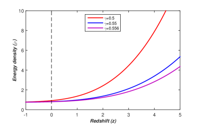
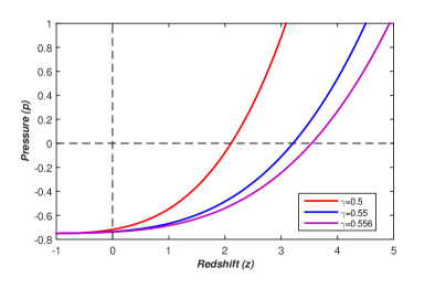
From above Eqs. (41) and (42), it is clear that $\rho\left(t\right)$ and $p\left(t\right)$ $\rightarrow\infty$ as $t\rightarrow 0$. 2 shows the behavior of the energy density of the Universe in terms of redshift for different values of $\gamma$. We can see that the variations of energy density versus redshift $z$ remains positive throughout the evolution of the Universe and is an increasing function of $z$, or, equivalently, a decreasing function of cosmic time $t$. It is initiated with a positive value and approaches to zero as $t\rightarrow\infty$ (i.e. $z\rightarrow-1$). As for pressure, its behavior is shown in Fig. 2, and is shown to be an increasing function of $z$, which starts from a large positive value and tends to a negative value in the present and future era. In reality, the negative pressure represents the accelerating expansion of the present Universe. Thus, the Bianchi type-I space-time is consistent with recent observational data of the Universe. Along with in this analysis, we fix the said values of the model constants parameter throughout the analysis: $m=0.5$, $n=0.6$, $\alpha=0.1$, and $\beta=1.5$.

Using Eqs. (41) and (42), the EoS parameter of Bianchi type-I space-time is obtained as

$$\omega\left(t\right)=\frac{p\left(t\right)}{\rho\left(t\right)}=-\frac{6\alpha\left[1+3\gamma^{2}\left(1-\frac{2}{\sqrt{3}\gamma}\right)\right]H^{2}\left(t\right)+4\alpha\left(1-\sqrt{3}\gamma\right)\overset{.}{H}\left(t\right)+\beta}{6\alpha\left(1-3\gamma^{2}\right)H^{2}\left(t\right)+\beta}.$$ (43)

$\omega=0$	dust
$\omega=\frac{1}{3}$	radiation
$\omega\in\left(-\frac{1}{3},-1\right)$	quintessence
$\omega=-1$	cosmological constant
$\omega<-1$	phantom matter

Table 1: Various values of the EoS parameter.

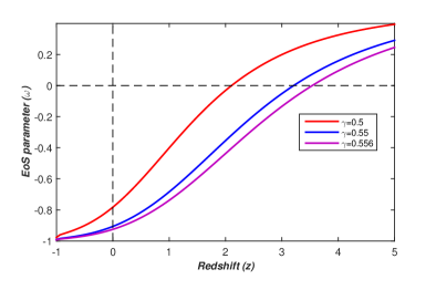
The EoS parameter is a very effective tool to study the evolutionary history of the Universe, and we can summarize in the Tab. 1 the different values taken by the EoS parameter and its corresponding region. From Eq. (43), we have observed that the EoS parameter of Bianchi type-I space-time is time-dependent. The graphical behavior of the EoS parameter versus redshift $z$ is shown in Fig; 3. From this figure, we see that the model starts in radiation dominated region, after which it passes from the matter region and varies in the quintessence region, and finally, it achieves $\Lambda CDM$ model for the values of $\gamma=0.5,0.55,0.556$. In standard model $\left(\Lambda CDM\right)$, the Universe evolves from the primordial phase dominated by photons, $\omega\sim\frac{1}{3}$, followed by the period of the dominance of dust matter with $\omega=0$. Finally, the cosmological constant dominates the Universe $\omega\rightarrow-1$ for large values of time. Thus, the Bianchi type-I model corresponds to the $\Lambda CDM$ model. Also, the current values of the EoS parameter for the three values of $\gamma$ are remarkably consistent with the most recent Planck measurements (see Tab. 2) [40].

Figure 3: The EoS parameter in terms of redshift for different values of $\gamma$.

$\gamma$	$\omega\left(z=0\right)$
$0.5$	$-0.7827$
$0.55$	$-0.9065$
$0.556$	$-0.9255$

Table 2: The current values of the EoS parameter for the three values of $\gamma$.

IV Analysis of stability and energy conditions

Analysis of stability through the squared sound speed:

The squared sound speed $\left(v_{s}^{2}\right)$ is exploited for examining the stability of the DE models which is given as $v_{s}^{2}=\frac{dp\left(t\right)}{d\rho\left(t\right)}$. If $v_{s}^{2}>0$, we obtain a stable model and if $v_{s}^{2}<0$, we obtain unstable model. For Bianchi type-I model, we observed the squared speed of sound, $v_{s}^{2}$ of the form

$$v_{s}^{2}=-\frac{6\alpha\left[1+3\gamma^{2}\left(1-\frac{2}{\sqrt{3}\gamma}\right)\right]\overset{.}{H}\left(t\right)H\left(t\right)+2\alpha\left(1-\sqrt{3}\gamma\right)\overset{..}{H}\left(t\right)}{6\alpha\left(1-3\gamma^{2}\right)H\left(t\right)\overset{.}{H}\left(t\right)}$$ (44)

where $\overset{..}{H}\left(t\right)=\frac{2n}{t^{3}}$.

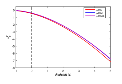
Fig. 4 shows the behavior of the squared speed of sound $v_{s}^{2}$ in terms of redshift for different values of $\gamma$, and it can be noted from this figure that the Bianchi type-I model is unstable throughout the cosmic evolution.

Figure 4: The squared sound speed $\left(v_{s}^{2}\right)$  in terms of redshift for different values of $\gamma$.

Energy conditions:

The energy conditions are useful linear relationships composed of energy density and pressure generated from the Raychaudhuri’s equation. They are important tools for validating dark energy models and are defined as follows [20]:

• Weak energy conditions (WEC): $\rho\geq 0$,

• Null energy condition (NEC): $\rho+p\geq 0$,

• Dominant energy conditions (DEC): $\rho-p\geq 0$,

• Strong energy conditions (SEC): $\rho+3p\geq 0$.

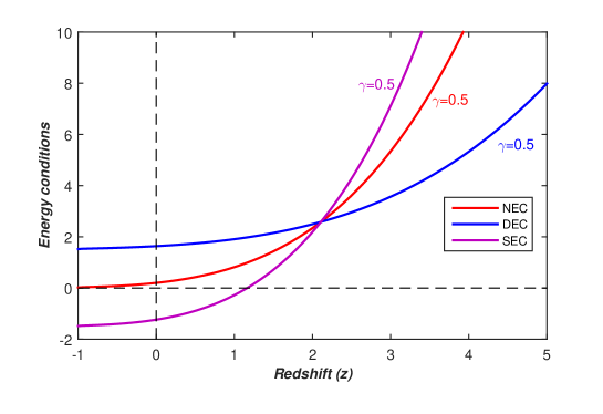
In Fig. 5 we can see the evolution of energy conditions NEC, DEC, and SEC in terms of redshift. In order to explicate the late-time cosmic acceleration with $\omega\simeq-1$, the SEC is necessary to violate i.e. $\rho\left(1+3\omega\right)\leq 0$. It is clearly shown by Fig. 5 that this condition is being violated in the present era and in the future.

Figure 5: The energy conditions in terms of redshift for $\gamma=0.5$.

V Cosmological parameters in terms of redshift

In the previous sections we have plotted the behavior of all physical parameters in terms of redshift $z$, in fact we used here the relationship between the scale factor and the redshift, which is expressed by

$$a\left(t\right)=\frac{a\left(t_{0}\right)}{1+z},$$ (45)

where $a\left(t_{0}\right)$ is the present scale factor.

For our model, we find the time-redshift relation in the form [38]

$$t\left(z\right)=\frac{nW\left[\frac{m\left(\frac{1}{1+z}\right)^{\frac{1}{n}}}{n}\right]}{m},$$ (46)

where $W$ denotes the Lambert function (also known as “product logarithm”).

The deceleration parameter is the quantity that describes the evolution of the expansion of the Universe. This parameter is positive $\left(q>0\right)$ when the Universe decelerates over time, and is negative $\left(q<0\right)$ in an accelerated expanding Universe. This parameter is related to the Hubble parameter as follows $q=-1-\frac{\overset{.}{H}}{H^{2}}$. Thus, the Hubble parameter and deceleration parameter of our model in terms of redshift are respectively obtained as

$$H\left(z\right)=\frac{m}{W\left[\frac{m\left(\frac{1}{1+z}\right)^{\frac{1}{n}}}{n}\right]}+m.$$ (47)

$$q\left(z\right)=-1+\frac{1}{n\left(1+W\left[\frac{m\left(\frac{1}{1+z}\right)^{\frac{1}{n}}}{n}\right]\right)^{2}}.$$ (48)

From (48), we observe that

$$q < 0\ \ if\ \ t>\frac{\sqrt{m}-m}{n},$$ (49)

$$q > 0\ \ if\ \ t<\frac{\sqrt{m}-m}{n}.$$

Figure 6: The deceleration parameter in terms of redshift.

Figure 7: The Hubble parameter in terms of redshift.

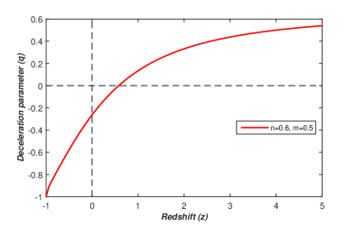
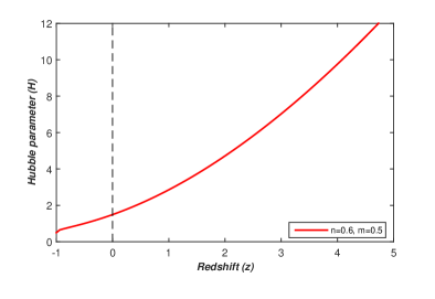
Recent observations of SN-Ia revealed that the Universe in the current era is accelerating and that the deceleration parameter value is in the range $-1\leq q<0$. Figs. 6 and 7 show the variation of Hubble parameter $H\left(z\right)$ and deceleration parameter $q\left(z\right)$ versus redshift $z$. It can be seen from Fig. LABEL:fig that $q\left(z\right)$ decreases from positive to negative zone and finally tends to $-1$. Thus, our model shows a transition from decelerated phase to an accelerated phase. Also, the value of the deceleration parameter is consistent with the observational data.

VI best fit values of model parameters from observation ($H(z)$ datasets)

As the cosmological principle on the large scale, universe is homogeneous and isotropic be the backbone of modern cosmology which had been tested several times by the researchers and supported by many cosmological observations. In this study, the expansion scenario of the universe be directly investigated by the Hubble parameter as a function of redshift. To measure the value of the Hubble parameter at some definite redshift generally two well-known methods such as the extraction of H(z) from line-of-sight BAO data and the differential age method are used [41]. In order to find the best fit value of the model parameters of our obtained model, we have used the technique of $57$ points of Hubble parameter values $H(z)$ with $\sigma_{\mu}^{2}$ errors of differential age method ($31$ points) and $BAO$ and other methods ($26$ points). Through the scale factor proposed in this model given in Eq. (33), we find its expression at the present time as $a_{0}=e^{mt_{0}}t_{0}^{n}$ where $t_{0}$ represent the present age of the Universe. Thus, after a simple calculation, we find the scale factor for our model as follows: $a(t)=a_{0}e^{k\left(\frac{t}{t_{0}}-1\right)}\left(\frac{t}{t_{0}}\right)^{n}$ where $k=mt_{0}$. The Hubble parameter in terms of redshift of our model with recent modification reads as

$$H(z)=\frac{H_{0}k}{k+n}\left[W^{-1}\left(\frac{k}{n}e^{\frac{k-ln(1+z)}{n}}\right)+1\right]$$ (50)

where $H_{0}=\frac{k+n}{t_{0}}$. We see from the above equation that the model parameters consist of three parameters $k,n$ and $H_{0}$ which will be constrained hereinafter by the last observations of Hubble datasets. The corresponding $\chi$-square function to obtain the best adjustment value for the parameters $k,n$ and $H_{0}$ is determined by

$$\chi_{OHD}^{2}(k,n,H_{0})=\sum_{\mu=1}^{57}\frac{\left[H_{th}(k,n,H_{0},z_{\mu})-H_{obs}(z_{\mu})\right]^{2}}{\sigma_{\mu}^{2}}$$ (51)

where $H_{th}(k,n,H_{0},z_{\mu})$ and $H_{obs}(z_{\mu})$ are theoretical and observed values of Hubble parameter respectively, and $\sigma_{\mu}^{2}$ represents the standard error in the observed Hubble parameter measurements. $\sigma_{\mu}^{2}$ errors of differential age method ($31$ points) and $BAO$ and other methods ($26$ points) are represented in Tab. III.

$z$	$H(z)$	$\sigma_{H}$	$z$	$H\left(z\right)$	$\sigma_{H}$
0.070	69	19.6	0.4783	80	99
0.90	69	12	0.480	97	62
0.120	68.6	26.2	0.593	104	13
0.170	83	8	0.6797	92	8
0.1791	75	4	0.7812	105	12
0.1993	75	5	0.8754	125	17
0.200	72.9	29.6	0.880	90	40
0.270	77	14	0.900	117	23
0.280	88.8	36.6	1.037	154	20
0.3519	83	14	1.300	168	17
0.3802	83	13.5	1.363	160	33.6
0.400	95	17	1.430	177	18
0.4004	77	10.2	1.530	140	14
0.4247	87.1	11.2	1.750	202	40
0.4497	92.8	12.9	1.965	186.5	50.4
0.470	89	34
$z$	$H\left(z\right)$	$\sigma_{H}$	$z$	$H\left(z\right)$	$\sigma_{H}$
0.24	79.69	2.99	0.52	94.35	2.64
0.30	81.7	6.22	0.56	93.34	2.3
0.31	78.18	4.74	0.57	87.6	7.8
0.34	83.8	3.66	0.57	96.8	3.4
0.35	82.7	9.1	0.59	98.48	3.18
0.36	79.94	3.38	0.60	87.9	6.1
0.38	81.5	1.9	0.61	97.3	2.1
0.40	82.04	2.03	0.64	98.82	2.98
0.43	86.45	3.97	0.73	97.3	7.0
0.44	82.6	7.8	2.30	224	8.6
0.44	84.81	1.83	2.33	224	8
0.48	87.90	2.03	2.34	222	8.5
0.51	90.4	1.9	2.36	226	9.3

Table 3: 57 points of $H(z)$ data: $31$ (DA) and $26$ (BAO+other) [41].

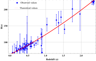
Now, using $57$ Hubble parameter measurements we will try to find the best fit values for the parameters model $k,n$ and $H_{0}$ where the best fit curve for the Hubble parameter versus redshift $z$ is represented in Fig. LABEL:fig8. Thus, The best fit values are gained as $k=0.2239\pm 0.3201$, $n=0.6886\pm 0.2868$ and $H_{0}=62.73\pm 8.43$ $km.s^{-1}.Mpc^{-1}.$

Figure 8: Best fit curve of Hubble function $H(z)$ vs. redshift $z$.

VII Conclusion and discussion

In this analysis, we have investigated an anisotropic Bianchi type-I space-time with perfect fluid in the framework of $f\left(Q\right)$ gravity, where $Q$ is the non-metricity scalar. Motivated by the work of Solanki et al. [31] we choose the $f\left(Q\right)$ function on the linear form, i.e. $f\left(Q\right)=\alpha Q+\beta$, where $\alpha$ and $\beta$ are free model parameters. We have used the ratio between the shear scalar and the expansion scalar is constant i.e. $\frac{\sigma}{\theta}=\gamma$. Here, we have examined the behavior of our model for three different values of $\gamma=0.5,0.55,0.556$.

It is observed that the metric potentials $A\left(t\right)$ and $B\left(t\right)$ vanish at the initial time (at $t=0$), and diverge at $t\rightarrow\infty$. Thus, the model obtains the initial singularity and predicts a big rip in the future. From Fig. 2, we see that the energy density of the Bianchi type-I Universe is a positive and decreasing function of cosmic time. Also, $\rho\rightarrow const$ as $t\rightarrow\infty$, which leads the fact that the volume of the space increases because of the density of matter decreases as the Universe expands in our model. The pressure in Fig. 2 takes negative values in the present and future eras, and this produces the current phase of the acceleration of the Universe, which is governed by dark energy. In Fig. 3, we can see that the Universe is dominated by radiation $\left(\omega\sim\frac{1}{3}\right)$ in the first epoch, and later it passes from the matter-dominated dust epoch $\left(\omega=0\right)$ to the Quintessence region $\omega\in\left(-\frac{1}{3},-1\right)$ and finally reaches the cosmological constant $\Lambda$ phase which causes the acceleration cosmic i.e. $\omega=-1$. We conclude that the model behaves like the standard cosmological model. To compare the current values of the EoS parameter obtained with this model with the recent Hubble measurements, we mention that Aghanim et al. [39] found constraint for the EoS parameter as follows:

• $\omega=-1.56_{-0.84}^{+0.60}$ (Planck + TT + lowE),

• $\omega=-1.58_{-0.41}^{+0.52}$ (Planck + TT, EE + lowE),

• $\omega=-1.57_{-0.40}^{+0.50}$ (Planck + TT, TE, EE + lowE + lensing),

• $\omega=-1.04_{-0.10}^{+0.10}$ (Planck + TT, TE, EE + lowE + lensing + BAO).

In Tab. II we provided the observed values in the derived model which are in excellent agreement with the above values.

In Section 4 we have examined the behavior of energy conditions in terms of the redshift of a Bianchi type-I space-time and found that WEC and NEC are all satisfied but SEC is violated. This leads directly to the creation of an accelerating phase of the Universe because $\rho\left(1+3\omega\right)<0$ results in that $\omega\simeq-1$, which corresponds to the observations. Further, for constraining the model parameter we have used Hubble data data sets ($57$ points of Hubble parameter values $H(z)$ see Tab. III). Hence, from the Hubble datasets, we have the best fit ranges for the model parameters are $k=0.2239\pm 0.3201$, $n=0.6886\pm 0.2868$ and $H_{0}=62.73\pm 8.43$.
Also, we have discussed the analysis of stability using the squared sound speed $\left(v_{s}^{2}\right)$ and found that the model is unstable throughout cosmic evolution i.e. $v_{s}^{2}<0$. In Figs.s 6 and 7, we draw the evolution of the deceleration parameter and the Hubble parameter in terms of the redshift, and it appears that the model passes from the deceleration phase to the current accelerated phase, and in the latter, it yields to $-1$. This result is consistent with the observational data of recent Planck measurements.

References

- [1] Einstein, Albert. ”The general theory of relativity.” The Meaning of Relativity. Springer, Dordrecht, 1922. 54-75.
- [2] Shapiro, Irwin I. ”Fourth test of general relativity.” Physical Review Letters 13.26 (1964): 789.
- [3] Bertotti, Bruno, Luciano Iess, and Paolo Tortora. ”A test of general relativity using radio links with the Cassini spacecraft.” Nature 425.6956 (2003): 374-376.
- [4] Will, Clifford M. ”The confrontation between general relativity and experiment.” Living reviews in relativity 17.1 (2014): 1-117.
- [5] Ricci, M. M. G., and Tullio Levi-Civita. ”Méthodes de calcul différentiel absolu et leurs applications.” Mathematische Annalen 54.1 (1900): 125-201.
- [6] Collaboration, Planck, et al. ”Planck 2013 results. XVI. Cosmological parameters.” A&A 571 (2014): A16.
- [7] Perlmutter, Saul, et al. ”Measurements of and from 42 high-redshift supernovae.” The Astrophysical Journal 517.2 (1999): 565.
- [8] Tonry, John L., et al. ”Cosmological results from high-z supernovae.” The Astrophysical Journal 594.1 (2003): 1.
- [9] Zlatev, Ivaylo, Limin Wang, and Paul J. Steinhardt. ”Quintessence, cosmic coincidence, and the cosmological constant.” Physical Review Letters 82.5 (1999): 896.
- [10] Nojiri, S. I., and S. D. Odintsov. ”eConf C0602061, 06 (2006).” Int. J. Geom. Meth. Mod. Phys 4.115 (2007): 16.
- [11] Nojiri, Shin’ichi, and Sergei D. Odintsov. ”Unified cosmic history in modified gravity: from theory to Lorentz non-invariant models.” Physics Reports 505.2-4 (2011): 59-144.
- [12] Koussour, M., and Bennai, M. ”Stability analysis of anisotropic Bianchi type-I cosmological model in teleparallel gravity.” Class. Quantum Gravity (2022).
- [13] Cai, Yi-Fu, et al. ” teleparallel gravity and cosmology.” Reports on Progress in Physics 79.10 (2016): 106901.
- [14] Koussour, M., et al. ”Holographic dark energy in Gauss-Bonnet gravity with Granda-Oliveros cut-off.” Nuclear Physics B 978 (2022): 115738..
- [15] Jiménez, Jose Beltrán, Lavinia Heisenberg, and Tomi Koivisto. ”Coincident general relativity.” Physical Review D 98.4 (2018): 044048.
- [16] Xu, Yixin, et al. ” gravity.” The European Physical Journal C 79.8 (2019): 1-19.
- [17] Albuquerque, Inês S., and Noemi Frusciante. ”A designer approach to gravity and cosmological implications.” Physics of the Dark Universe 35 (2022): 100980.
- [18] Solanki, Raja, Avik De, and P. K. Sahoo. ”Complete dark energy scenario in gravity.” Physics of the Dark Universe 36 (2022): 100996.
- [19] Jiménez, Jose Beltrán, et al. ”Cosmology in geometry.” Physical Review D 101.10 (2020): 103507.
- [20] Mandal, Sanjay, P. K. Sahoo, and J. R. L. Santos. ”Energy conditions in gravity.” Physical Review D 102.2 (2020): 024057.
- [21] Mandal, Sanjay, Deng Wang, and P. K. Sahoo. ”Cosmography in gravity.” Physical Review D 102.12 (2020): 124029.
- [22] Khyllep, Wompherdeiki, Andronikos Paliathanasis, and Jibitesh Dutta. ”Cosmological solutions and growth index of matter perturbations in gravity.” Physical Review D 103.10 (2021): 103521.
- [23] Beh, Jing-Theng, Tee-How Loo, and Avik De. ”Geodesic deviation equation in gravity.” Chinese Journal of Physics (2021).
- [24] Harko, Tiberiu, et al. ”Coupling matter in modified gravity.” Physical Review D 98.8 (2018): 084043.
- [25] Dimakis, N., A. Paliathanasis, and T. Christodoulakis. ”Quantum cosmology in theory.” Classical and Quantum Gravity 38.22 (2021): 225003.
- [26] Shekh, S. H. ”Models of holographic dark energy in gravity.” Physics of the Dark Universe 33 (2021): 100850.
- [27] De, Avik, et al. ”Isotropization of locally rotationally symmetric Bianchi-I universe in -gravity.” The European Physical Journal C 82.1 (2022): 1-11.
- [28] Lazkoz, Ruth, et al. ”Observational constraints of gravity.” Physical Review D 100.10 (2019): 104027.
- [29] Frusciante, Noemi. ”Signatures of gravity in cosmology.” Physical Review D 103.4 (2021): 044021.
- [30] Barros, Bruno J., et al. ”Testing gravity with redshift space distortions.” Physics of the Dark Universe 30 (2020): 100616.
- [31] Zhao, Dehao. ”Covariant formulation of theory.” The European Physical Journal C 82.4 (2022): 1-12.
- [32] Collins, C. Barry, and Stephen W. Hawking. ”Why is the universe isotropic?.” The Astrophysical Journal 180 (1973): 317-334.
- [33] Collins, C. B., E. N. Glass, and D. A. Wilkinson. ”Exact spatially homogeneous cosmologies.” General Relativity and Gravitation 12.10 (1980): 805-823.
- [34] Bunn, Emory F., Pedro G. Ferreira, and Joseph Silk. ”How anisotropic is our universe?.” Physical Review Letters 77.14 (1996): 2883.
- [35] Harko, T., and M. K. Mak. ”Viscous Bianchi type I universes in brane cosmology.” Classical and Quantum Gravity 20.3 (2003): 407.
- [36] Harko, T., and M. K. Mak. ”Anisotropy in Bianchi-type brane cosmologies.” Classical and Quantum Gravity 21.6 (2004): 1489.
- [37] Rodrigues, M. E., et al. ”Locally rotationally symmetric Bianchi type-I cosmological model in gravity: from early to dark energy dominated universe.” International Journal of Modern Physics D 23.01 (2014): 1450004.
- [38] Moraes, P. H. R. S., and P. K. Sahoo. ”The simplest non-minimal matter–geometry coupling in the cosmology.” The European Physical Journal C 77.7 (2017): 1-8.
- [39] Solanki, Raja, et al. ”Accelerating expansion of the universe in modified symmetric teleparallel gravity.” arXiv preprint arXiv:2201.06521 (2022).
- [40] Collaboration, Planck, et al. ”Planck 2018 results. VI. Cosmological parameters.” (2020).
- [41] Stern D. et al., ”constraining the equation of state of dark energy.” J. Cosmol. Astropart. Phys. 02, (2010) 008.
- [42] Sharov, G. S., and V. O. Vasiliev. ”How predictions of cosmological models depend on Hubble parameter data sets.” arXiv preprint arXiv:1807.07323 (2018).