First-Order Logic Axiomatization of Metric Graph Theory

Jérémie Chalopin, Manoj Changat, Victor Chepoi, and Jeny Jacob

Aix-Marseille Université, CNRS, Université de Toulon, LIS, Marseille, France

{jeremie.chalopin,victor.chepoi}@lis-lab.fr

University of Kerala, Department of Futures Studies, Trivandum, India

{mchangat,jenyjacobktr}@gmail.com

Abstract. The main goal of this note is to provide a First-Order Logic with Betweenness (FOLB) axiomatization of the main classes of graphs occurring in Metric Graph Theory, in analogy to Tarski’s axiomatization of Euclidean geometry. We provide such an axiomatization for weakly modular graphs and their principal subclasses (median and modular graphs, bridged graphs, Helly graphs, dual polar graphs, etc), basis graphs of matroids and even $\Delta$-matroids, partial cubes and their subclasses (ample partial cubes, tope graphs of oriented matroids and complexes of oriented matroids, bipartite Pasch and Peano graphs, cellular and hypercellular partial cubes, almost-median graphs, netlike partial cubes), and Gromov hyperbolic graphs. On the other hand, we show that some classes of graphs (including chordal, planar, Eulerian, and dismantlable graphs), closely related with Metric Graph Theory, but defined in a combinatorial or topological way, do not allow such an axiomatization.

1. Introduction

First-Order Logic (FOL) is the language of classical logic most widely used in various areas of mathematics and computer science. First-order logic uses quantified variables over non-logical objects and allows the use of sentences that contain variables. The first-order language of graph theory is defined in the usual way with variables ranging over the vertex-set and the edge relation as the primitive relation. However, not many graph properties can be expressed using this logic: such fundamental properties as Connectivity, Acyclicity, Bipartiteness, Planarity, Eulerian, and Hamiltonian Path are not first-order definable on finite graphs [114, 160]. Therefore developing a comprehensive first-order theory on graphs with more expressive power is an important problem. A possible approach towards such a theory is to transpose to graphs Tarski’s axiomatic approach to Euclidean geometry [157, 158, 147].

Tarski developed a First-Order Logic theory of Euclidean geometry using only “points” as the “primitive geometric objects” in contrast to other theories of Euclidean geometry of Hilbert and Birkhoff, where points, lines, planes, etc., are all primitive “geometrical objects”. In Tarski’s theory, there are two primitive geometrical relations (predicats): the ternary relation $B$ of “betweenness” and the quaternary relation $\equiv$ of “equidistance” or “congruence of segments”. The elegance of Tarski’s axiomatic theory of geometry is that the axiom system admits elimination of quantifiers: that is, every formula is provably equivalent (on the basis of the axioms) to a Boolean combination of basic formulas. The theory is complete: every assertion is either provable or refutable; the theory is decidable – there is a mechanical procedure for determining whether or not any given assertion is provable and also there is a constructive consistency proof for the theory. Tarski’s axioms are an axiom set for the substantial fragment of Euclidean geometry that is formulable in first-order logic with identity, and requiring no set theory [157, 158, 147].

The main goal of this article is the First-Order Logic axiomatization of Metric Graph Theory using the notion of Betweenness, in a similar vein as Tarski’s First-Order Logic approach to Euclidean geometry. The natural betweenness on graphs is the metric betweenness (or shortest path betweenness) resulting from the standard path metric $d$ of connected graphs $G=(V,E)$ and defined using the ternary relation $\operatorname{B}(abc)$ on the vertex set $V$ of a graph $G$ meaning that “the vertex $b$ lies on some shortest path of $G$ between the vertices $a$ and $c$”. We abbreviate the Fist Order Logic with Betweenness of graphs by FOLB.

The main subject of Metric Graph Theory (MGT) is the investigation and characterization of graph classes whose metric satisfies main properties of classical metric geometries like Euclidean $\ell_{2}$-geometry (and more generally, the $\ell_{1}$- and $\ell_{\infty}$-geometries), hyperbolic spaces, hypercubes, trees. Such central properties are convexity of balls, Helly property for balls, geometry of geodesic or metric triangles, isometric and low-distortion embeddings, the retractions, the four-point conditions, uniqueness or existence of medians, etc. The main classes of graphs central to MGT are median graphs, Helly graphs, partial cubes and ${\ell}_{1}$–graphs, bridged graphs, graphs with convex balls, Gromov hyperbolic graphs, modular and weakly modular graphs. Other classes surprisingly arise from combinatorics and geometry: basis graphs of matroids, even $\Delta$-matroids, tope graphs of oriented matroids, dual polar spaces. For a survey of classes arising in MGT, see the survey [14]). For a theory of weakly modular graphs and their subclasses, see the paper [50] and for partial cubes and $\ell_{1}$-graphs, see the books [80] and [99].

In this paper, we show that all these graph classes occurring in MGT are definable in FOLB. On the other hand, we show that chordal graphs, dismantlable graphs, Eulerian graphs, planar graphs, and partial Johnson graphs are not definable in FOLB. Chordal graphs form a subclass of bridged graphs, dismantlable graphs form a superclass of bridged and Helly graphs, partial Johnson graphs generalize partial cubes. Since often the FOLB-definability of a graph class is based not on its initial definition but on a characterization, which is not the principal or nicest one, when we introduce a graph class we define it, briefly motivate its importance, and present the used characterization. Then we refer to mentioned above papers and books or to other references for a more detailed treatment of each class. Notice that many of the classes from metric graph theory contain all trees but not all cycles; they are often defined by forbidding isometric subgraphs and cycles of given lengths. Consequently, these classes cannot be defined in the standard First Order Logic on graphs: indeed, the proof establishing that $\operatorname*{\sf Acyclicity}$ is not FOL-definable immediately implies that such classes are not FOL-definable.

The paper is organized as follows. In Section 2 we present the main basic definitions about graphs and First Order Logic. We also recall the Ehrenfeucht-Fraïssé games as the tool of proving that some queries are not definable in FOL for graphs. In Section 3 we introduce the First Order Logic with Betweenness for graphs and give the first examples of queries which are definable in this logic. In Section 4 we show that weakly modular graphs and their main subclasses and super-classes occurring in Metric Graph Theory are FOLB-definable. In Section 5 we show FOLB-definability of partial cubes and some of their subclasses and super-classes. Section 6 is devoted to FOLB-definability of Gromov hyperbolic graphs. In Section 7, we establish that some classes of graphs are not FOLB-definable. In Section 8, we explain how such FOLB characterization lead to polynomial time recognition algorithms.

2. Preliminaries

In this section, we recall the main definitions about graphs and the first-order logic. In the three subsections about first-order logic we closely follow the paper [114] by Kolaitis (we also use the book by Libkin [118]).

2.1. Graphs

A graph $G=(V,E)$ consists of a set of vertices $V:=V(G)$ and a set of edges $E:=E(G)\subseteq V\times V$. All graphs considered in this paper are finite, undirected, connected, and contain no multiple edges nor loops. For two distinct vertices $v,w\in V$ we write $v\sim w$ (respectively, $v\nsim w$) when there is an (respectively, there is no) edge connecting $v$ with $w$, that is, when $vw:=\{v,w\}\in E$. For vertices $v,w_{1},\ldots,w_{k}$, we write $v\sim w_{1},\ldots,w_{k}$ (respectively, $v\nsim w_{1},\ldots,w_{k}$) or $v\sim A$ (respectively, $v\nsim A$) when $v\sim w_{i}$ (respectively, $v\nsim w_{i}$), for each $i=1,\ldots,k$, where $A=\{w_{1},\ldots,w_{k}\}$. As maps between graphs $G=(V,E)$ and $G^{\prime}=(V^{\prime},E^{\prime})$ we always consider simplicial maps, that is functions of the form $f\colon V\to V^{\prime}$ such that if $v\sim w$ in $G$ then $f(v)=f(w)$ or $f(v)\sim f(w)$ in $G^{\prime}$. A $(u,w)$–path $(v_{0}=u,v_{1},\ldots,v_{k}=w)$ of length $k$ is a sequence of vertices with $v_{i}\sim v_{i+1}$. If $k=2,$ then we call $P$ a 2-path of $G$. If $v_{i}\neq v_{j}$ for $|i-j|\geq 1$, then $P$ is called a simple $(a,b)$–path. A $k$–cycle $(v_{0},v_{1},\ldots,v_{k-1})$ is a path $(v_{0},v_{1},\ldots,v_{k-1},v_{0})$. For a subset $A\subseteq V,$ the subgraph of $G=(V,E)$ induced by $A$ is the graph $G(A)=(A,E^{\prime})$ such that $uv\in E^{\prime}$ if and only if $uv\in E$ ($G(A)$ is sometimes called a full subgraph of $G$). A square $uvwz$ (respectively, triangle $uvw$, pentagon $uvwxz$) is an induced $4$–cycle $(u,v,w,z)$ (respectively, $3$–cycle $(u,v,w)$, $5$-cycle $(u,v,w,x,z)$).

The distance $d(u,v)=d_{G}(u,v)$ between two vertices $u$ and $v$ of a graph $G$ is the length of a shortest $(u,v)$–path. For a vertex $v$ of $G$ and an integer $r\geq 1$, we denote by $B_{r}(v,G)$ (or by $B_{r}(v)$) the ball in $G$ (and the subgraph induced by this ball) of radius $r$ centered at $v$, that is, $B_{r}(v,G)=\{x\in V:d(v,x)\leq r\}.$ More generally, the $r$–ball around a set $A\subseteq V$ is the set (or the subgraph induced by) $B_{r}(A,G)=\{v\in V:d(v,A)\leq r\},$ where $d(v,A)=\mbox{min}\{d(v,x):x\in A\}$. As usual, $N(v)=B_{1}(v,G)\setminus\{v\}$ denotes the set of neighbors of a vertex $v$ in $G$. A graph $G=(V,E)$ is isometrically embeddable into a graph $H=(W,F)$ if there exists a mapping $\varphi:V\rightarrow W$ such that $d_{H}(\varphi(u),\varphi(v))=d_{G}(u,v)$ for all vertices $u,v\in V$. More generally, for an integer $k\geq 1$, a graph $G=(V,E)$ is scale $k$ embeddable into a graph $H=(W,F)$ if there exists a mapping $\varphi:V\rightarrow W$ such that $d_{H}(\varphi(u),\varphi(v))=k\cdot d_{G}(u,v)$ for all vertices $u,v\in V$. A retraction $\varphi$ of a graph $G$ is an idempotent nonexpansive mapping of $G$ into itself, that is, $\varphi^{2}=\varphi:V(G)\rightarrow V(G)$ with $d(\varphi(x),\varphi(y))\leq d(x,y)$ for all $x,y\in W$. The subgraph of $G$ induced by the image of $G$ under $\varphi$ is referred to as a retract of $G$.

The interval $I(u,v)$ between $u$ and $v$ consists of all vertices on shortest $(u,v)$–paths, that is, of all vertices (metrically) between $u$ and $v$: $I(u,v)=\{x\in V:d(u,x)+d(x,v)=d(u,v)\}.$ If $d(u,v)=2$, then $I(u,v)$ is called a 2-interval. A 2-interval $I(u,v)$ is called thick if $I(u,v)$ contains two non-adjacent vertices $x,y\in I(u,v)\setminus\{u,v\}$. A graph $G$ is called thick if all 2-intervals of $G$ are thick. A subgraph of $G$ (or the corresponding vertex-set $A$) is called convex if it includes the interval of $G$ between any pair of its vertices. The smallest convex subgraph containing a given subgraph $S$ is called the convex hull of $S$ and is denoted by conv$(S)$. A halfspace is a convex set of $G$ whose complement is convex. An induced subgraph $H$ (or the corresponding vertex-set of $H$) of a graph $G$ is gated if for every vertex $x$ outside $H$ there exists a vertex $x^{\prime}$ in $H$ (the gate of $x$) such that $x^{\prime}\in I(x,y)$ for any $y$ of $H$. Gated sets are convex and the intersection of two gated sets is gated. By Zorn’s lemma there exists a smallest gated subgraph containing a given subgraph $S$, called the gated hull of $S$.

Let $G_{i}$, $i\in\Lambda$ be an arbitrary family of graphs. The Cartesian product $\prod_{i\in\Lambda}G_{i}$ is a graph whose vertices are all functions $x:i\mapsto x_{i}$, $x_{i}\in V(G_{i})$ and two vertices $x,y$ are adjacent if there exists an index $j\in\Lambda$ such that $x_{j}y_{j}\in E(G_{j})$ and $x_{i}=y_{i}$ for all $i\neq j$. Note that a Cartesian product of infinitely many nontrivial graphs is disconnected. Therefore, in this case the connected components of the Cartesian product are called weak Cartesian products. The direct product $\boxtimes_{i\in\Lambda}G_{i}$ of graphs $G_{i}$, $i\in\Lambda$ is a graph having the same set of vertices as the Cartesian product and two vertices $x,y$ are adjacent if $x_{i}y_{i}\in E(G_{i})$ or $x_{i}=y_{i}$ for all $i\in\Lambda$.

We continue with the definition of some graphs. The complete graph on $n$ vertices is denote by $K_{n}$ and the complete bipartite graph with parts of size $n$ and $m$ by $K_{n,m}$. The wheel $W_{k}$ is a graph obtained by connecting a single vertex – the central vertex $c$ – to all vertices of the $k$–cycle $(x_{1},x_{2},\ldots,x_{k})$; the almost wheel $W_{k}^{-}$ is the graph obtained from $W_{k}$ by deleting a spoke (i.e., an edge between the central vertex $c$ and a vertex $x_{i}$ of the $k$–cycle). Analogously $K^{-}_{4}$ and $K^{-}_{3,3}$ are the graphs obtained from $K_{4}$ and $K_{3,3}$ by removing one edge. An $n$–octahedron $K_{n\times 2}$ (or, a hyperoctahedron, for short) is the complete graph $K_{2n}$ on $2n$ vertices minus a perfect matching. A hypercube $Q_{m}$ of dimension $m$ is a graph having the subsets of a set $X$ of size $m$ as vertices and two such sets $A,B$ are adjacent in $Q_{m}$ if and only if $|A\triangle B|=1$. A halved cube $\frac{1}{2}Q_{m}$ has the vertices of a hypercube $Q_{m}$ corresponding to subsets of $X$ of even cardinality as vertices and two such vertices are adjacent in $\frac{1}{2}Q_{m}$ if and only if their distance in $Q_{m}$ is 2 (analogously one can define a halved cube on finite subsets of odd cardinality). For a positive integer $k$, the Johnson graph $J(m,k)$ has the subsets of $X$ of size $k$ as vertices and two such vertices are adjacent in $J(m,k)$ if and only if their distance in $Q_{m}$ is $2$. All Johnson graphs $J(m,k)$ with even $k$ are isometric subgraphs of the halved cube $\frac{1}{2}Q_{m}$ and the halved cube $\frac{1}{2}Q_{m}$ is scale 2 embedded in the hypercube $Q_{m}$. The hypercube $Q_{m}$ can be viewed as the Cartesian product of $m$ copies of $K_{2}$. The Hamming graph $H_{m_{1},\ldots,m_{d}}$ is a Cartesian product of the complete graphs $K_{m_{1}},\ldots K_{m_{d}}$.

2.2. First-Order Logic (FOL)

In this subsection we recall the main definitions from First-Order Logic. A vocabulary $\sigma=(P_{1},\ldots,c_{1},\ldots,c_{s})$ consists of a set of constant symbols and a set of relation symbols (called also predicates) of specified arities. Given a vocabulary $\sigma$, the variables and the constant symbols are the $\sigma$-terms. The set of formulas is defined inductively as follows:

• given terms $t_{1},\ldots,t_{k}$ and a $k$-ary predicate $P$, then $P(t_{1},\ldots,t_{k})$ is a formula;;

• for each formulas $F,F^{\prime}$, $\neg F,(F\wedge F^{\prime})$, and $F\vee F^{\prime})$ are formulas;

• if $F$ is a formula and $x$ is a variable, then $\exists xF$ and $\forall xF$ are formulas.

Atomic formulas are those constructed according to the first rule. A general first-order formula is build up from atomic formulas using Boolean connectives and the two quantifiers. Given a vocabulary $\sigma$, a $\sigma$-structure is a tuple $\mathbf{A}=(A,P^{\mathbf{A}}_{1},\ldots,P^{\mathbf{A}}_{m},c^{\mathbf{A}}_{1},\ldots c^{\mathbf{A}}_{1})$ consisting of

• a non-empty set $A$, called the universe;

• for each constant $c_{i}$, an element $c^{\mathbf{A}}_{i}$ of $A$;

• for each $k$-ary predicate $P_{i}$ in $\sigma$, a $k$-ary relation $P^{\mathbf{A}}_{i}\subset\underbrace{A\times\cdots\times A}_{k}$.

A finite $\sigma$-structure is a $\sigma$-structure $\mathbf{A}$ whose universe $A$ is finite.

Let $\mathbf{A}=(A,P^{\mathbf{A}}_{1},\ldots,P^{\mathbf{A}}_{m},c^{\mathbf{A}}_{1},\ldots,c^{\mathbf{A}}_{s})$ and $\mathbf{B}=(B,P^{\mathbf{B}}_{1},\ldots,P^{\mathbf{B}}_{m},c^{\mathbf{B}}_{1},\ldots,c^{\mathbf{B}}_{s})$ be two $\sigma$-structures. An isomorphism between $\mathbf{A}$ and $\mathbf{B}$ is a mapping $h:A\rightarrow B$ that satisfies the following conditions:

• $h$ is a one-to-one and onto function;

• for every constant symbol $c_{j},j=1,\ldots,s$, we have $h(c^{\mathbf{A}}_{j})=c^{\mathbf{B}}_{j}$;

• for each relation symbol $P_{i},i=1,\ldots,m$, of arity $t$ and any $t$-tuple $(a_{1},\ldots,a_{t})$ from $A$, we have $P^{\mathbf{A}}_{i}(a_{1},\ldots,a_{t})$ if and only if $P^{\mathbf{B}}_{i}(h(a_{1}),\ldots,h(a_{t}))$.

Given two structures $\mathbf{A}=(A,P^{\mathbf{A}}_{1},\ldots,P^{\mathbf{A}}_{m},c^{\mathbf{A}}_{1},\ldots,c^{\mathbf{A}}_{s})$ and $\mathbf{B}=(B,P^{\mathbf{B}}_{1},\ldots,P^{\mathbf{B}}_{m},c^{\mathbf{B}}_{1},\ldots,c^{\mathbf{B}}_{s})$, $\mathbf{B}$ is a substructure of $\mathbf{A}$ if $B\subseteq A$, each $P^{\mathbf{B}}_{i}$ is the restriction of $P^{\mathbf{A}}_{i}$ to $B$ (which means that $P^{\mathbf{B}}_{i}=P^{\mathbf{A}}_{i}\cap B^{t}$) and $c^{\mathbf{B}}_{j}=c^{\mathbf{A}}_{j},j=1,\ldots,s$. If $\mathbf{A}$ is a $\sigma$-structure and $D$ is a subset of $A$, then the substructure of $\mathbf{A}$ generated by $D$ is the structure $\mathbf{A}\upharpoonright D$ having the set $D\cup\{c^{\mathbf{A}}_{1},\ldots,c^{\mathbf{A}}_{s}\}$ as its universe and having the restrictions of the relations $P^{\mathbf{A}}_{i}$ on $D\cup\{c^{\mathbf{A}}_{1},\ldots,c^{\mathbf{A}}_{s}\}$ as its relations. A partial isomorphism from $\mathbf{A}$ to $\mathbf{B}$ is an isomorphism from a substructure of $\mathbf{A}$ to a substructure of $\mathbf{B}$. Given a structure $\mathbf{A}$, a variable $x$, and $a\in A$, the structure $\mathbf{A}_{[x\mapsto a]}$ is the same as $\mathbf{A}$ except that $x^{\mathbf{A}_{[x\rightarrow a]}}=a$.

Example 1.

A (undirected) graph is a $\sigma$-structure $\mathbf{G}=(V,E)$ with the vertex-set $V$ as the universe and the vocabulary $\sigma$ with one binary relation symbol $E$, where $E$ is interpreted as the edge relation. The subgraph of $\mathbf{G}$ induced by a set of vertices $D$ of $\mathbf{G}$ is the substructure of $\mathbf{G}$ generated by $D$.

Let $\mathbf{A}$ be a $\sigma$-structure with universe $A$. The value $\mathbf{A}[t]$ of each term $t$ is an element of the universe $A$, inductively defined as follows:

• for a constant symbol $c$, set $\mathbf{A}[c]=c^{\mathbf{A}}$;

• for a variable $x$, set $\mathbf{A}[x]=x^{\mathbf{A}}$;

• for a term $f(t_{1},\ldots,f_{k})$, where $f$ is a $k$-ary function symbol and $t_{1},\ldots,t_{k}$ are terms, set $\mathbf{A}[f(t_{1},\ldots,t_{k})]=f^{\mathbf{A}}(\mathbf{A}[t_{1}],\ldots,\mathbf{A}[t_{k}])$.

The satisfaction relation $\mathbf{A}\vDash F$ (which means that $\mathbf{A}$ satisfies $F$ or that $\mathbf{A}$ models F) between a $\sigma$-structure $\mathbf{A}$ and $\sigma$-formula $F$ is defined by induction over the structure of $F$:

• $\mathbf{A}\vDash P(t_{1},\ldots,t_{k})$ if and only if $(\mathbf{A}[t_{1}],\ldots,\mathbf{A}[t_{k}])\in P^{\mathbf{A}}$;

• $\mathbf{A}\vDash(F\wedge F^{\prime})$ if and only if $\mathbf{A}\vDash F$ and $\mathbf{A}\vDash F^{\prime}$;

• $\mathbf{A}\vDash(F\vee F^{\prime})$ if and only if $\mathbf{A}\vDash F$ or $\mathbf{A}\vDash F^{\prime}$;

• $\mathbf{A}\vDash\neg F$ if and only if $\mathbf{A}\nvDash F$;

• $\mathbf{A}\vDash\exists xF$ if and only if there exists $a\in A$ such that $\mathbf{A}_{[x\mapsto a]}\vDash F$;

• $\mathbf{A}\vDash\forall xF$ if and only if $\mathbf{A}_{[x\mapsto a]}\vDash F$ for all $a\in A$;

• $\mathbf{A}\vDash t_{1}=t_{2}$ if and only if $\mathbf{A}[t_{1}]=\mathbf{A}[t_{2}]$.

A first-order formula $F$ over signature $\sigma$ is satisfiable if $\mathbf{A}\vDash F$ for some $\sigma$-structure $\mathbf{A}$. If $F$ is not satisfiable it is called unsatisfiable. $F$ is called valid if $\mathbf{A}\vDash F$ for every $\sigma$-structure $\mathbf{A}$.

Following the terminology of [114, 118], we continue with the concept of query, one of the most fundamental concepts in finite model theory. Let $\sigma$ be a vocabulary. A class of $\sigma$-structures is a collection $\mathcal{C}$ of $\sigma$-structures that is closed under isomorphisms. A $k$-ary query on $\mathcal{C}$ is a mapping $Q$ with domain $\mathcal{C}$ such that $Q$ is preserved under isomorphisms and $Q(\mathbf{A})$ is a $k$-ary relation on $\mathbf{A}$ for all $\mathbf{A}\in\mathcal{C}$. A Boolean query on $\mathcal{C}$ is a mapping $Q:\mathcal{C}\rightarrow\{0,1\}$ that is preserved under isomorphisms. Consequently, $Q$ can be identified with the subclass $\mathcal{C}^{\prime}=\{\mathbf{A}\in\mathcal{C}:Q(\mathbf{A})=1\}$ of $\mathcal{C}$. For example, the $\operatorname*{\sf Connectivity}$ query on graphs $\mathbf{G}=(V,E)$ is the Boolean query such that $\operatorname*{\sf Connectivity}(\mathbf{G})=1$ if and only if the graph $\mathbf{G}$ is connected. Queries are mathematical objects that formalize the concept of a “property” of structures and makes it possible to define what means for such a “property” to be expressible in some logic.

Let $L$ be a (first-order) logic and $\mathcal{C}$ a class of $\sigma$-structures. A $k$-ary query $Q$ on $\mathcal{C}$ is $L$-definable if there exists a formula $F(x_{1},\ldots,x_{k})$ of $L$ with $x_{1},\ldots,x_{k}$ as free variables and such that for every $\mathbf{A}\in\mathcal{C}$, $Q(\mathbf{A})=\{(a_{1},\ldots,a_{k})\in A^{k}:\mathbf{A}\vDash F(a_{1},\ldots,a_{k})\}$. A Boolean query $Q$ on $\mathcal{C}$ is $L$-definable if there exists an $L$-formula $F$ such that for every $\mathbf{A}\in\mathcal{C}$, $Q(\mathbf{A})=1$ if and only if $\mathbf{A}\vDash F$. Let $L(\mathcal{C})$ denotes the collection of all $L$-definable queries on $\mathcal{C}$.

The expressive power of a logic $L$ on a class $\mathcal{C}$ of finite structures is defined by the collection of $L$-definable queries on $\mathcal{C}$, i.e., is to determine which queries on $\mathcal{C}$ are $L$-definable and which are not. To show that a query $Q$ is definable, it suffices to find some $L$-formula that defines it on every structure in $\mathcal{C}$. In contrast, showing that $Q$ is not $L$-definable entails showing that no formula of $L$ defines the property. One of the main tools in proving that a query is not definable in first-order logic of finite graphs is the method of Ehrenfeucht-Fraïssé games, defined in the next subsection.

2.3. Ehrenfeucht-Fraïssé games

Let $r$ be a positive integer, $\sigma$ a vocabulary, and $\mathbf{A}$ and $\mathbf{B}$ two $\sigma$-structures. The $r$-move Ehrenfeucht-Fraïssé game on $\mathbf{A}$ and $\mathbf{B}$ is played between two players, called the Spoiler and the Duplicator. Each run of the game has $r$ moves. In each move, the Spoiler plays first and picks an element from the universe $A$ of $\mathbf{A}$ or from the universe $B$ of $\mathbf{B}$; the Duplicator then responds by picking an element of the other structure (i.e., if Spoiler picked an element from $A$, then the Duplicator picks and element from $B$, and vice versa). Let $a_{i}\in A$ and $b_{i}\in B$ be the two elements picked by the Spoiler and the Duplicator in their $i$-th move, $1\leq i\leq r$.

• The Duplicator wins the run $(a_{1},b_{1}),\ldots,(a_{r},b_{r})$ if the mapping $a_{i}\mapsto b_{i},i=1,\ldots,r$ and $c_{j}^{\mathbf{A}}\mapsto c_{j}^{\mathbf{B}},j=1,\ldots,s$ is a partial isomorphism from $\mathbf{A}$ to $\mathbf{B}$, which means that it is an isomorphism between the substructure $\mathbf{A}\upharpoonright\{a_{1},\ldots,a_{r}\}$ of $\mathbf{A}$ restricted to $\{a_{1},\ldots,a_{r}\}$ and the substructure $\mathbf{B}\upharpoonright\{b_{1},\ldots,b_{r}\}$ of $\mathbf{B}$ restricted to $\{b_{1},\ldots,b_{r}\}$. otherwise, the Spoiler wins the run $(a_{1},b_{1}),\ldots,(a_{r},b_{r})$.

• The Duplicator wins the $r$-move Ehrenfeucht-Fraïssé game on $\mathbf{A}$ and $\mathbf{B}$ if the Duplicator can win every run of the game, i.e., if (s)he has a winning strategy for the Ehrenfeucht-Fraïssé game. Otherwise, the Spoiler wins the $r$-move Ehrenfeucht-Fraïssé game.

• We write $\mathbf{A}\sim_{r}B$ to denote that the Duplicator wins the $r$-move Ehrenfeucht-Fraïssé game on $\mathbf{A}$ and $\mathbf{B}$.

From this definition follows that $\sim_{r}$ is an equivalence relation on the class of all $\sigma$-structures. For a formal definition of the winning strategy for the Duplicator, see for example [114, Definition 3.4]. Ehrenfeucht-Fraïssé games characterize definability in first-order logic. To describe this connection, we need the following definition.

Let $F$ be a first-order formula over a vocabulary $\sigma$. The quantifier rank of $F$, denoted by $\operatorname*{qr}(F)$, is defined inductively in the following way:

• if $F$ is atomic, then $\operatorname*{qr}(F)=0$;

• if $F$ is of the form $\neg F^{\prime}$, then $qr(F)=\operatorname*{qr}(F^{\prime})$;

• if $F$ is of the form $F^{\prime}\vee F^{\prime\prime}$ or of the form $F^{\prime}\wedge F^{\prime\prime}$, then $\operatorname*{qr}(F)=\max\{\operatorname*{qr}(F^{\prime}),\operatorname*{qr}(F^{\prime\prime})\}$;

• if $F$ is of the form $\exists xF^{\prime}$ or of the form $\forall xF^{\prime}$, then $\operatorname*{qr}(F)=\operatorname*{qr}(F^{\prime})+1$.

For a positive integer $r$ and two $\sigma$-structures $\mathbf{A}$ and $\mathbf{B}$, $A\equiv_{r}\mathbf{B}$ denotes that $\mathbf{A}$ and $\mathbf{B}$ satisfy the same first-order sentences of quantifier rank $r$; $\equiv_{r}$ is an equivalence relation on the class of all $\sigma$-structures. The main result of Ehrenfeucht and Fraïssé asserts that the equivalence relations $\equiv_{r}$ and $\sim_{r}$ coincide:

Theorem 2 (​[87, 90]).

Let $r$ be a positive integer and let $\mathbf{A}$ and $\mathbf{B}$ be two $\sigma$-structures. Then the following two conditions are equivalent:

• $\mathbf{A}\equiv_{r}\mathbf{B}$, i.e., $\mathbf{A}$ and $\mathbf{B}$ have the same first-order sentences of quantifier rank $r$;

• $\mathbf{A}\sim_{r}\mathbf{B}$, i.e., the Duplicator wins the $r$-move Ehrenfeucht-Fraïssé game on $\mathbf{A}$ and $\mathbf{B}$.

Moreover, $\equiv_{r}$ has finitely many equivalence classes and each $\equiv_{r}$-equivalence class is definable by a first-order sentence of quantified rank $r$.

For a proof of this theorem, see [114]. A consequence of this theorem is the following result:

Theorem 3.

Let $\mathcal{C}$ be a class of $\sigma$-structures and $Q$ be a Boolean query on $\mathcal{C}$. Then the following statements are equivalent:

• $Q$ is first-order definable on $\mathcal{C}$;

• there exists a positive integer $r$ such that, for every $\mathbf{A},\mathbf{B}\in\mathcal{C}$, if $Q(\mathbf{A})=1$ and the Duplicator wins the $r$-move Ehrenfeucht-Fraïssé game on $\mathbf{A}$ and $\mathbf{B}$, then $Q(\mathbf{B})=1$.

This theorem provides the following method for studying first-order definability of Boolean queries on classes of $\sigma$-structures. Let $\mathcal{C}$ be a $\sigma$-structure and $Q$ be a Boolean query on $\mathcal{C}$. To show that $Q$ is not first-order definable on $\mathcal{C}$, it suffices to show that for every positive integer $r$ there are $\mathbf{A}_{r},\mathbf{B}_{r}\in\mathcal{C}$ such that

• $Q(\mathbf{A}_{r})=1$ and $Q(\mathbf{B}_{r})=0$;

• the Duplicator wins the $r$-move Ehrenfeucht-Fraïssé game on $\mathbf{A}$ and $\mathbf{B}$.

The method is also complete, i.e., if $Q$ is not first-order definable on $\mathcal{C}$, then for every positive integer $r$ such structures $\mathbf{A}_{r}$ and $\mathbf{B}_{r}$ exist.

2.4. What can be expressed and what cannot be expressed in FOL for graphs

Recall that an undirected graph is a $\sigma$-structure $\mathbf{G}=(V,E)$ with the universe $V$ and the vocabulary $\sigma$ with one binary relation symbol $\operatorname{E}$ (interpreted as the edge relation) such that $\operatorname{E}(u,v)\Rightarrow\operatorname{E}(v,u)$ and $(\forall u)(\neg\operatorname{E}(u,u))$. We start with a few queries on graphs, which are first-order definable:

Example 4.

Let $H=(V^{\prime},E^{\prime})$ be a graph with vertex-set $V^{\prime}=\{1,\ldots,p\}$. The Boolean query ${\operatorname*{\sf Subgraph}}_{H}$ meaning “$\mathbf{G}$ contains $H$ as an induced subgraph” is definable by the first-order formula

$${\operatorname*{\sf Subgraph}}_{H}\equiv(\exists v_{1})(\exists v_{2})\cdots(\exists v_{p})(\bigwedge_{ij\in E^{\prime}}\operatorname{E}(v_{i},v_{j})\wedge\bigwedge_{ij\notin E^{\prime}}\neg\operatorname{E}(v_{i},v_{j})).$$

This implies that the query $\operatorname*{\sf Subgraph}_{H_{1},\ldots,H_{p}}$ meaning “$\mathbf{G}$ contains at least one of the graphs $H_{1},\ldots,H_{p}$ as an induced subgraph” is also first-order definable.

Analogously, the binary query “there exists a path of length $k$ from $x$ to $y$” is definable by the first order formula

$$\varphi_{k}(x,y):=(\exists v_{1})(\exists v_{2})\cdots(\exists v_{k-1})(\operatorname{E}(x,v_{1})\wedge\operatorname{E}(v_{1},v_{2})\wedge\cdots\wedge\operatorname{E}(v_{k-2},v_{k-1})\wedge\operatorname{E}(v_{k-1},y)).$$

Using the formulas $\varphi_{k}$, one can show that the binary query $\operatorname*{\sf dist}_{\leq k}(x,y)$ meaning that “the distance between $x$ and $y$ is at most $k$” is definable by the first order formula

$${\operatorname*{\sf dist}}_{\leq k}(x,y)\equiv\varphi_{k}(x,y)\vee\varphi_{k-1}(x,y))\vee\cdots\vee\varphi_{1}(x,y)\vee(x=y).$$

The binary query $\operatorname*{\sf dist}_{k}(x,y)$ meaning that “the distance between $x$ and $y$ is at most $k$” can then be defined as the first order formula

$${\operatorname*{\sf dist}}_{k}(x,y)\equiv{\operatorname*{\sf dist}}_{\leq k}(x,y)\wedge\neg{\operatorname*{\sf dist}}_{\leq k-1}(x,y).$$

Using the last queries, one can easily show that the Boolean queries $\operatorname*{\sf Isometric}_{H}$ and $\operatorname*{\sf Isometric}_{H_{1},\ldots,H_{p}}$ meaning “$\mathbf{G}$ contains $H$ as an isometric subgraph” and “$\mathbf{G}$ contains at least one of the graphs $H_{1},\ldots,H_{p}$ as an isometric subgraph” are also first-order definable. For example, if $H$ is a graph with the vertex-set $\{1,\ldots,p\}$, then $\operatorname*{\sf Isometric}_{H}$ is definable by the formula

$${\operatorname*{\sf Isometric}}_{H}\equiv(\exists v_{1})(\exists v_{2})\cdots(\exists v_{p})\left(\bigwedge_{k=1}^{p}\left(\bigwedge_{\{i,j\}:d_{H}(i,j)=k}{\operatorname*{\sf dist}}_{k}(v_{i},v_{j})\right)\right).$$

On the other hand, the most queries on graphs are not first-order definable, in particular the following well-known queries:

• The $\operatorname*{\sf Acyclicity}$ query is the Boolean query such that $\operatorname*{\sf Acyclicity}(\mathbf{G})=1$ iff $\mathbf{G}$ is an acyclic graph;

• The $\operatorname*{\sf Bipartite}$ query is the Boolean query such that $\operatorname*{\sf Bipartite}(\mathbf{G})=1$ iff $\mathbf{G}$ is a bipartite graph;

• The $\operatorname*{\sf Connectivity}$ query is the Boolean query such that $\operatorname*{\sf Connectivity}(\mathbf{G})=1$ iff $G$ is a connected graph;

• The $\operatorname*{\sf Even}$ query is the Boolean query such that $\operatorname*{\sf Even}(\mathbf{G})=1$ iff $\mathbf{G}$ has an even number of vertices.

All these results can be obtained via Ehrenfeucht-Fraïssé games [114, 118].

3. First Order Logic with Betweenness (FOLB)

In this section, we introduce the first-order logic with betweenness. Betweenness was first formulated in geometry and nowadays has a rich history. Euclid, Pasch, Hilbert, Peano, and Tarski studied betweeness in Euclidean geometry axiomatically. Menger [122] and Blumenthal [41] investigated metric betweeness, i.e., betweenness in general metric spaces. Inspired by the work of Pasch, Pitcher and Smiley [135] and Sholander [148, 149, 150] were the first to investigate betweenness in the discrete setting: in lattices, partial orders, trees, and median semilattices. In graphs, the study of metric betweenness was initiated by Mulder [125]. Prenowitz and Jantosciak [141] were the first to investigate the notion of betweenness in the setting of abstract convexity by introducing the concept of join space. Hedliková represented the betweenness relation as a ternary relation and introduced the concept of ternary space; the betweenness relation in a ternary space unifies the metric, order and lattice betweenness. Finally, this led to the equivalent concept of geometric interval space [162].

3.1. Betweenness and interval spaces

Let $X$ be any finite set. For each pair $u,v$ of points in $X$, let $uv$ be a subset of $X$, called the interval between $u$ and $v$. Then $X$ is a (finite) interval space [162] if and only if

1. $u\in uv$;

2. $uv=vu$;

Every interval space gives rise to a betweenness relation: we will say that a point $x$ is between the points $u$ and $v$ (notation $uxv$) if $x\in uv$. The interval space $X$ is said to be geometric if it satisfies the following three conditions for all $u,v,w,x\in X$ [27, 163]:

1. $uu=\{u\}$,

2. $w\in uv$ implies $uw\subseteq uv$,

3. $v,w\in ux$ and $v\in uw$ implies $w\in vx$.

A particular instance of geometric interval space is any metric space $(X,d)$: the intervals are the metric intervals $uv=\{x\in X:d(u,x)+d(x,v)=d(u,v)\}$.

For each point $u$ one defines the base-point relation at $u$ as follows: $x\leq_{u}y$ if and only if $x\in uy$. The next lemma summarizes an equivalent description of geometric interval spaces [162, Section 27]:

Lemma 1.

An interval space $X$ is geometric if and only if it satisfies the following conditions:

1. $w\in ux$ and $x\in uw$ implies $w=x$;

2. $v\in uw$ and $w\in ux$ implies $v\in ux$ and $w\in vx$;

3. for each point $u$ the base-point relation $\leq_{u}$ is a partial order such that for any $v\leq_{u}w$ we have $vw=\{x:v\leq_{u}x\leq_{u}w\}$.

Let $X$ be any set together with a ternary relation $uxv$. If $u,w,v\in X$ and $uwv$, then $w$ is said to be between $u$ and $v$. The interval $uv$ is defined as the set of all $w\in X$ between $u$ and $v$. A ternary space (which can be equally called a space with betweenness) is a set $X$ together with a ternary relation $uxv$ satisfying the following conditions [100]:

1. $uwv$ implies $vwu$;

2. $uwv$ and $uvw$ implies $v=w$;

3. $uwv$ and $uvx$ implies $wvx$ and $uwx$.

From Lemma 1 it follows that a geometric interval space is exactly a ternary space satisfying the property that $u\in uv$ (i.e., $uuv$) for all $u,v\in X$.

An interval $uv$ of an interval space $X$ is called an edge if $u\neq v$ and $uv=\{u,v\}$; the edges then form the graph $G(X)$ of the interval space $X$.

Lemma 2 (​[9]).

Let $X$ be a finite geometric interval space. Then the graph $G(X)$ of $X$ is connected.

The graph $G(X)$ of a finite geometric interval space $X$ can be regarded as a metric space, where the standard graph-metric $d$ accounts the lengths of shortest paths in the graph. We denote by $I(u,v)=\{x\in X:x\mbox{ on a shortest path between }u\mbox{ and }v\}$ the corresponding intervals in $G(X)$ which have to be distinguished from the intervals $uv$ in $X$. An interval space $X$ is called graphic [9, 162] if the equality $uv=I(u,v)$ holds for all points $u,v$ of the space.

A simple sufficient condition for a finite interval space to be graphic was given in [9]. An interval space $X$ is said to satisfy the triangle condition if for any three points $u,v,w$ in $X$ with

1. $uv\cap uw=\{u\},uv\cap vw=\{v\},$ and $uw\cap vw=\{w\}$, the intervals $uv,uw,vw$ are edges whenever at least one of them is an edge.

Theorem 5 (​[9]).

A finite geometric interval space $X$ satisfying the axiom (ITC) is graphic.

Graphic interval spaces have been characterized by Mulder and Nebeský [126] (improving over the previous such characterizations obtained by Nebeský). Additionally, to axioms (I1)-(I5) of a geometric interval space, they require two additional axioms introduced in [129]:

1. $uu^{\prime}=\{u,u^{\prime}\},vv^{\prime}=\{v,v^{\prime}\},u\in u^{\prime}v^{\prime}$, and $u^{\prime},v^{\prime}\in uv$ imply $v\in u^{\prime}v^{\prime}$;

2. $uu^{\prime}=\{u,u^{\prime}\},vv^{\prime}=\{v,v^{\prime}\},u^{\prime}\in uv,v^{\prime}\notin uv$, and $v\notin u^{\prime}v^{\prime}$ imply $u^{\prime}\in uv^{\prime}$.

Theorem 6 (​[126]).

A finite geometric interval space $X$ is graphic if and only if it satisfies the axioms (I6) and (I7).

Observe that if $Y$ is a subset of an interval space $X$, we can define an interval structure on $Y$ by taking the intersection of the interval $uv$ in $X$ with $Y$ for any pair $u,v\in Y$. If $X$ is a graphic interval space, then $Y$ endowed with this inherited interval structure is also a graphic interval space. Note however that $G(Y)$ may be different from the subgraph of $G(X)$ induced by $Y$.

3.2. FOLB for graphs

Given a ternary predicate $B$ on a finite set $V$, we define the binary predicate $\operatorname{E}_{\operatorname{B}}$ on $V$ as follows: $\operatorname{E}_{\operatorname{B}}(u,v):=u\neq v\wedge\left(\operatorname{B}(u,x,v)\implies(x=u)\vee(x=v)\right)$.

A graphic interval structure is a $\sigma$-structure $(V,B)$ where $V$ is a finite set and $B$ is a ternary predicate on $V$ satisfying the following axioms:

1. $\forall u\forall v\operatorname{B}(u,u,v)$

2. $\forall u\forall v\forall x\operatorname{B}(u,x,v)\implies\operatorname{B}(v,x,u)$

3. $\forall u\forall x\operatorname{B}(u,x,u)\implies x=u$

4. $\forall u\forall v\forall w\forall x\operatorname{B}(u,w,v)\wedge\operatorname{B}(u,x,w)\implies\operatorname{B}(u,x,v)$

5. $\forall u\forall v\forall w\forall x\operatorname{B}(u,v,x)\wedge\operatorname{B}(u,w,x)\wedge\operatorname{B}(u,v,w)\implies\operatorname{B}(v,w,x)$

6. $\forall u\forall u^{\prime}\forall v\forall v^{\prime}\operatorname{E}_{\operatorname{B}}(u,u^{\prime})\wedge\operatorname{E}_{\operatorname{B}}(v,v^{\prime})\wedge\operatorname{B}(u^{\prime},u,v^{\prime})\wedge\operatorname{B}(u,u^{\prime},v)\wedge\operatorname{B}(u,v^{\prime},v)\implies\operatorname{B}(u^{\prime},v,v^{\prime})$

7. $\forall u\forall u^{\prime}\forall v\forall v^{\prime}\operatorname{E}_{\operatorname{B}}(u,u^{\prime})\wedge\operatorname{E}_{\operatorname{B}}(v,v^{\prime})\wedge\operatorname{B}(u,u^{\prime},v)\wedge\neg\operatorname{B}(u,v^{\prime},v)\wedge\neg\operatorname{B}(u^{\prime},v,v^{\prime})\implies\operatorname{B}(u,u^{\prime},v^{\prime})$.

Observe that since $B$ satisfies (IB2), $G_{\operatorname{B}}=(V,E_{\operatorname{B}})$ is an undirected graph seen as a $\sigma^{\prime}$-structure (as defined in Section 2.4). By Lemma 2, $G_{\operatorname{B}}$ is a connected graph. Since $B$ satisfies (IB1)–(IB7), by Theorem 6, for any $u,v,x\in V$, $x\in I_{G_{\operatorname{B}}}(u,v)$ if and only if $\operatorname{B}(u,x,v)$. When $\operatorname{B}(u,x,v)$ is true, it means that $x$ belongs to the interval $I_{G_{\operatorname{B}}}(u,v)$.

When considering the class $\mathcal{C}$ of $\sigma$-structures $(V,B)$ satisfying axioms (IB1)–(IB7), we say that a query $Q$ on $\mathcal{C}$ is definable in first order logic with betweeness (FOLB-definable) if it can be defined by a first order formula $F$ over $(V,B)$.

Observe that by the definition of $\operatorname{E}_{\operatorname{B}}$, any FOL-definable query is also FOLB-definable. In particular the queries $\operatorname*{\sf dist}_{k}$ and $\operatorname*{\sf dist}_{\leq k}$ are FOLB-definable.

3.3. What can be expressed in FOLB for graphs: first results

There are properties in FOLB that cannot be expressed using only FOL. Namely, we prove that $\operatorname*{\sf Bipartite}$ and $\operatorname*{\sf Tree}$ are FOLB-definable, where $\operatorname*{\sf Tree}$ is $\operatorname*{\sf Acyclicity}\wedge\operatorname*{\sf Connectivity}$. Since in FOLB we consider only connected graphs, $\operatorname*{\sf Connectivity}$ is a trivial query in FOLB.

A graph is bipartite if and only if for any edge $uv$ and any vertex $x$, the distances from $x$ to $u$ and to $v$ are different, and thus if and only if either $u\in I_{G}(x,v)$ or $v\in I_{G}(x,u)$. Consequently, $\operatorname*{\sf Bipartite}$ is definable by the following FOLB-formula:

$$\operatorname*{\sf Bipartite}\equiv\left(\forall u\forall v\forall x\operatorname{E}_{\operatorname{B}}(u,v)\implies\operatorname{B}(x,u,v)\vee\operatorname{B}(x,v,u)\right).$$

A tree is bipartite. In a bipartite connected graph, if $G$ is not a tree, there are two vertices $u,x$ such that $u$ has two neighbors in the interval $I_{G}(u,x)$. Indeed, consider a cycle $C$ and an arbitrary vertex $x$. Let $u$ be the vertex of $C$ that is the furthest from $x$. Since $G$ is bipartite, the two neighbors $v,w$ of $x$ on $C$ belong to the interval $I(x,u)$. Consequently, $\operatorname*{\sf Tree}$ is definable by the following FOLB-formula:

$$\operatorname*{\sf Tree}\equiv\left(\operatorname*{\sf Bipartite}\wedge\forall u\forall v\forall w\forall x\operatorname{E}_{\operatorname{B}}(u,v)\wedge\operatorname{E}_{\operatorname{B}}(u,w)\wedge\operatorname{B}(x,v,u)\wedge\operatorname{B}(x,w,u)\implies v=w\right).$$

We will use the predicates $\operatorname*{\sf triangle}(x,y,z)$, $\operatorname*{\sf square}(x,y,z,u),$ and $\operatorname*{\sf pentagon}(x,y,z,u,v)$, which are true if and only if the vertices $x,y,z$, $x,y,z,u$, and $x,y,z,u,v$ induce respectively a triangle, a square, or a pentagon of a graph $G$. We will also use the predicate $\operatorname*{\sf closest}(v,x,y)$, which is true if and only of the intervals $I(x,v)$ and $I(y,v)$ intersects only in the vertex $v$. $\operatorname*{\sf closest}(v,x,y)$ can be written as the FOLB-formula $(\forall v^{\prime}\operatorname{B}(x,v^{\prime},v)\wedge\operatorname{B}(y,v^{\prime},v)\implies v^{\prime}=v)$.

Given four vertices $u,v,x,y$ of $G$, the following predicate express that $x$ and $y$ belong to a common shortest path going from $u$ to $v$ (reaching first $x$ and then $y$):

$$\operatorname*{\sf colinear}(u,x,y,v)\equiv\operatorname{B}(u,x,v)\wedge\operatorname{B}(x,y,v)$$

Three vertices $x,y,z$ of a graph $G$ define a metric triangle $xyz$ [64] if $I(x,y)\cap I(x,z)=\{x\}$, $I(x,y)\cap I(y,z)=\{y\}$, and $I(x,z)\cap I(y,z)=\{z\}$. This can be expressed using the predicate

$$\operatorname*{\sf metric-triangle}(x,y,z)\equiv\operatorname*{\sf closest}(x,y,z)\wedge\operatorname*{\sf closest}(y,x,z)\wedge\operatorname*{\sf closest}(z,x,y).$$

The size of a metric triangle $xyz$ is $\max(d(x,y),d(x,z),d(y,z))$.

Given three vertices $x,y,z$, a metric triangle $x^{\prime}y^{\prime}z^{\prime}$ is a quasi-median of $x,y,z$ if $d(x,y)=d(x,x^{\prime})+d(x^{\prime},y^{\prime})+d(y^{\prime},y)$, $d(x,z)=d(x,x^{\prime})+d(x^{\prime},z^{\prime})+d(z^{\prime},z)$, and $d(y,z)=d(y,y^{\prime})+d(y^{\prime},z^{\prime})+d(z^{\prime},z)$, For any vertices $x,y,z$, one can obtain a quasi-median $x^{\prime}y^{\prime}z^{\prime}$ of $x,y,z$ by taking $x^{\prime}\in I(x,y)\cap I(x,z)$ furthest from $x$, $y^{\prime}\in I(x^{\prime},y)\cap I(y,z)$ furthest from $y$, and $z^{\prime}\in I(x^{\prime},z)\cap I(y^{\prime},z)$ furthest from $z$. It can be expressed by the following predicate:

$$\operatorname*{\sf quasi-median}(x,y,z,x^{\prime},y^{\prime},z^{\prime})\equiv \operatorname*{\sf metric-triangle}(x^{\prime},y^{\prime},z^{\prime})\wedge\operatorname*{\sf colinear}(x,x^{\prime},y^{\prime},y)$$

$$\wedge\operatorname*{\sf colinear}(x,x^{\prime},z^{\prime},z)\wedge\operatorname*{\sf colinear}(y,y^{\prime},z^{\prime},z).$$

A quasi-median $x^{\prime}y^{\prime}z^{\prime}$ of $x,y,z$ such that $x^{\prime}=y^{\prime}=z^{\prime}$ is called a median of $x,y,z$. Equivalently, $m$ belongs to $I(x,y)\cap I(x,z)\cap I(y,z)$.

$$\operatorname*{\sf median}(x,y,z,m) \equiv\operatorname*{\sf quasi-median}(x,y,z,m,m,m)$$

$$\equiv\operatorname{B}(x,m,y)\wedge\operatorname{B}(x,m,z)\wedge\operatorname{B}(y,m,z).$$

The following metric conditions on a graph $G$ play an important way in the definition of many graph classes:

• Triangle Condition ($\mathrm{TC}$): for any three vertices $v,x,y$ such that $d(v,x)=d(v,y)$ and $x\sim y$, there exists a vertex $z\in I(x,v)\cap I(y,v)$ such that $xzy$ is a triangle of $G$;

• Quadrangle Condition ($\mathrm{QC}$): for any four vertices $v,x,y,u$ such that $d(v,x)=d(v,y)=d(v,u)-1$ and $u\sim x,y$, $x\nsim y$, there exists a vertex $z\in I(x,v)\cap I(y,v)$ such that $xzyu$ is a square of $G$;

• Triangle-Pentagon Condition ($\mathrm{TPC}$): for any three vertices $v,x,y$ such that $d(v,x)=d(v,y)$ and $x\sim y$, either there exists a vertex $z\in I(x,v)\cap I(y,v)$ such that $xzy$ is a triangle of $G$, or there exist vertices $z,x^{\prime},y^{\prime}$ such that $xx^{\prime}zy^{\prime}y$ is a pentagon of $G$, $z\in I(x,v)\cap I(y,v)$, and $d(x,z)=d(y,z)=2$;

• Interval Neighborhood Condition ($\mathrm{INC}$): for any two distinct vertices $u,v\in V$, the neighbors of $u$ in $I(u,v)$ form a clique.

We denote the respective queries by $\operatorname*{\sf Triangle-Condition}$, $\operatorname*{\sf Quadrangle-Condition}$, $\operatorname*{\sf Pentagon-Condition}$, and $\operatorname*{\sf Interval-Neighborhood-Condition}$ and we show that these properties are FOLB-definable:

$$\operatorname*{\sf Triangle-Condition} \equiv\forall v\forall x\forall y\operatorname{E}_{\operatorname{B}}(x,y)\wedge\operatorname*{\sf closest}(v,x,y)\implies\operatorname*{\sf triangle}(x,y,v)$$

$$\operatorname*{\sf Quadrangle-Condition} \equiv\forall v\forall x\forall y\forall u\operatorname{E}_{\operatorname{B}}(u,x)\wedge\operatorname{E}_{\operatorname{B}}(u,y)\wedge\neg\operatorname{E}_{\operatorname{B}}(x,y)$$

$$\quad\wedge\operatorname{B}(u,x,v)\wedge\operatorname{B}(x,u,y)\wedge\operatorname{B}(u,y,v)\wedge\operatorname*{\sf closest}(v,x,y)$$

$$\quad\implies\operatorname*{\sf square}(u,x,v,y)$$

$$\operatorname*{\sf Triangle-Pentagon-Condition} \equiv\forall v\forall x\forall y\operatorname{E}_{\operatorname{B}}(x,y)\wedge\operatorname*{\sf closest}(v,x,y)\implies\operatorname*{\sf triangle}(x,y,v)$$

$$\quad\vee\exists x^{\prime}\exists y^{\prime}\operatorname*{\sf pentagon}(x,x^{\prime},v,y^{\prime},y)$$

$$\operatorname*{\sf Interval-Neighborhood-Condition} \equiv\forall u\forall v\forall x\forall y\operatorname{E}_{\operatorname{B}}(u,x)\wedge\operatorname{E}_{\operatorname{B}}(u,y)\wedge\operatorname{B}(u,x,v)\wedge\operatorname{B}(u,y,v)$$

$$\quad\implies\operatorname{E}_{\operatorname{B}}(x,y).$$

Observe that if a graph $G$ satisfies $\mathrm{INC}$, then $G$ does not contain any square. Moreover, when $G$ satisfies $\mathrm{QC}$, $G$ satisfies $\mathrm{INC}$ if and only if $G$ does not contain any square.

4. Weakly modular graphs, their subclasses and superclasses

In this section, we present the FOLB-definability of weakly modular graphs and their main subclasses and super-classes, which constitute an important part of Metric Graph Theory. Subclasses of weakly modular graphs are the following classes of graphs: median, modular, quasi-modular, quasi-median, pseudo-modular, weakly median, bridged and weakly bridged, Helly, dually polar, and sweakly modular. Meshed graphs constitute a super-class of weakly modular graphs. Basis graphs of matroids and of even $\Delta$-matroids are subclasses of meshed graphs.

4.1. Weakly modular graphs

Weakly modular graphs have been introduced in the papers [64] and [9]. A nice local-to-global theory of weakly modular graphs and their subclasses mentioned above has been developed in the recent paper [50]. For results about weakly modular graphs, the reader can consult the survey [14] and the paper [50].

A graph is weakly modular if it satisfies the triangle condition ($\mathrm{TC}$) and the quadrangle condition ($\mathrm{QC}$). Thus being weakly modular can be expressed by the following FOLB-query:

$$\textsf{Weakly Modular}\equiv\operatorname*{\sf Triangle-Condition}\wedge\operatorname*{\sf Quadrangle-Condition}.$$

In [64], weakly modular graphs have been characterized as graphs in which metric triangles $xyz$ are strongly equilateral, i.e., for any $u\in I(y,z)$, we have $d(x,u)=d(x,y)=d(x,z)$. In fact, this characterization leads to another FOLB query characterizing weakly modular graphs:

$$\operatorname*{\sf strongly-equilateral}(x,y,z) \equiv\forall u\forall v\operatorname{E}_{\operatorname{B}}(u,v)\implies$$

$$\quad\big{(}((\operatorname{B}(y,u,z)\wedge\operatorname{B}(y,v,z))\implies\neg(\operatorname{B}(x,u,v)\vee\operatorname{B}(x,v,u)))$$

$$\quad\wedge((\operatorname{B}(x,u,z)\wedge\operatorname{B}(x,v,z))\implies\neg(\operatorname{B}(y,u,v)\vee\operatorname{B}(y,v,u)))$$

$$\quad\wedge((\operatorname{B}(x,u,y)\wedge\operatorname{B}(x,v,y))\implies\neg(\operatorname{B}(z,u,v)\vee\operatorname{B}(z,v,u)))\big{)}$$

Strongly-Equilateral Triangles $$\equiv\forall x\forall y\forall z\operatorname*{\sf strongly-equilateral}(x,y,z)$$

The predicate $\operatorname*{\sf strongly-equilateral}(x,y,z)$ establishes that for any adjacent vertices $u,v$ of $I(y,z)$ (for $I(x,y)$ and $I(x,z)$, the arguments are similar), we have $u\notin I(x,v)$ and $v\notin I(x,u)$, yielding $d(x,u)=d(x,v)$. Consequently, the connectedness of $I(y,z)$ establishes that all vertices of $I(y,z)$ have the same distance to $x$. This shows that $\operatorname*{\sf strongly-equilateral}(x,y,z)$ is true if and only if $xyz$ is a strongly equilateral metric triangle.

$$\textsf{Weakly Modular}\equiv\textsf{Strongly-Equilateral Triangles}.$$

We say that a graph $G$ has equilateral metric triangles if every metric triangle $xyz$ of $G$ is equilateral, i.e., $d(x,y)=d(x,z)=d(y,z)$. One can ask if graphs with equilateral metric triangles are FOLB-definable.

A modular graph is a bipartite weakly modular graph, i.e., a bipartite graph satisfying the quadrangle condition. Thus being modular can be expressed by the following FOLB-queries:

Modular $$\equiv\operatorname*{\sf Bipartite}\wedge\textsf{Weakly Modular}$$

$$\equiv\operatorname*{\sf Bipartite}\wedge\operatorname*{\sf Quadrangle-Condition}.\$$

A graph is pseudo-modular [21] if it satisfies the triangle condition and if for any three vertices $v,x,y$ such that $d(x,y)=2$ and $d(v,x)=d(v,y)=k$, there exists a vertex $z\sim x,y$ such that $d(v,z)=k-1$. The second property can be viewed as a strengthening of the quadrangle condition. In fact, a graph is pseudo-modular if and only if all metric triangles have size at most $1$ and can thus be FOLB-defined by the following formula:

$$\textsf{Pseudo-Modular}\equiv\forall x\forall y\forall z\operatorname*{\sf metric-triangle}(x,y,z)\implies(x=y=z)\vee\operatorname*{\sf triangle}(x,y,z).$$

A quasi-modular graph is a $K_{4}^{-}$-free weakly modular graph [23] and thus being quasi-modular is a FOLB-definable property.

$$\textsf{Quasi-Modular}\equiv\textsf{Weakly Modular}\wedge\neg{\operatorname*{\sf Subgraph}}_{K_{4}^{-}}.$$

Quasi-modular graphs are pseudo-modular but the converse inclusion does not hold.

A graph $G=(V,E)$ is called meshed [14] if the following condition ($\mathrm{QC}^{-}$) is satisfied for any three vertices $v,x,y$ with $d(x,y)=2$: there exists a common neighbor $z$ of $x$ and $y$ such that $2d(v,z)\leq d(v,x)+d(v,y)$. This condition seems to be a relaxation, but it implies the triangle condition (that is not implied by the quadrangle condition). Conversely, ($\mathrm{TC}$) and ($\mathrm{QC}$) imply ($\mathrm{QC}^{-}$) and thus weakly modular graphs are meshed. In meshed graphs, any metric triangle $xyz$ is equilateral [12].

Lemma 3.

$G$ is a meshed graph if and only if for any metric triangle $vxy$, if $d(x,y)=2$, then $d(v,x)=d(v,y)=2$ and there exists $z\sim x,y$ such that $d(v,z)=2$.

Proof.

Let $G$ be a meshed graph and consider a metric triangle $vxy$ such that $d(x,y)=2$. Since metric triangles in meshed graphs are equilateral, we have $d(v,x)=d(v,y)=2$, and by ($\mathrm{QC}^{-}$), there exists $z\sim x,y$ such that $d(v,z)\leq 2$. If $d(v,z)=1$, then $z\in I(v,x)\cap I(v,y)\cap I(x,y)$ and thus $vxy$ is not a metric triangle. Consequently, $d(v,z)=2$.

Consider now a graph $G$ such that for any metric triangle $vxy$ of $G$ with $d(x,y)=2$, we have $d(v,x)=d(v,y)=2$ and there exists $z\sim x,y$ such that $d(v,z)=2$. We show that ($\mathrm{QC}^{-}$) holds in $G$. Consider three vertices $v,x,y$ such that $d(x,y)=2$ and let $v^{\prime}x^{\prime}y^{\prime}$ be a metric triangle such that $v^{\prime},x^{\prime}\in I(v,x)$, $v^{\prime},y^{\prime}\in I(v,y)$, and $x^{\prime},y^{\prime}\in I(x,y)$. If $x\neq x^{\prime}$, then either $x^{\prime}=y$ (if $y\in I(x,v)$) or $x^{\prime}\sim x,y$. In the first case, let $z$ be a common neighbor of $x$ and $y$ and in the second case, let $z=x^{\prime}$. In both cases, observe that $d(v,z)=d(v,x)-1\leq d(v,y)+1$ and thus ($\mathrm{QC}^{-}$) holds for $v,x,y$. We can thus assume now that $x=x^{\prime}$ and for similar reasons that $y=y^{\prime}$. Since $d(x,y)=2$, we know by hypothesis that $d(v^{\prime},x)=d(v^{\prime},y)=2$ and that there exists $z\sim x,y$ such that $d(v^{\prime},z)=2$. Consequently, $d(v,z)\leq d(v,v^{\prime})+d(v^{\prime},z)=d(v,v^{\prime})+2=d(v,v^{\prime})+d(v^{\prime},x)=d(v,x)=d(v,y)$ and thus ($\mathrm{QC}^{-}$) holds for $v,x,y$. ∎

Consequently, meshedness of a graph can be written as the following FOLB query:

Meshed $$\equiv\forall v\forall x\forall y\operatorname*{\sf metric-triangle}(v,x,y)\wedge{\operatorname*{\sf dist}}_{2}(x,y)\implies{\operatorname*{\sf dist}}_{2}(x,v)\wedge{\operatorname*{\sf dist}}_{2}(y,v)$$

$$\quad\wedge(\exists z\operatorname{E}_{\operatorname{B}}(x,z)\wedge\operatorname{E}_{\operatorname{B}}(y,z)\wedge{\operatorname*{\sf dist}}_{2}(z,v)).$$

The previous lemma establishes that meshed graphs are precisely the graphs in which every metric triangle $xyz$ of size $2$, there exists a common neighbor of $y$ and $z$ at distance $2$ from $x$. Therefore one can ask whether meshed graphs are exactly the graph where for each metric triangle $xyz$, $y$ and $z$ can be connected by a shortest path in which all vertices have the same distance to $x$.

4.2. Median graphs

Median graphs constitute the most important class of graphs in Metric Graph Theory. This is due to the occurrence of median graphs in completely different areas of mathematics and computer science. This is also due to their deep and rich combinatorial and geometric structure, which was an inspiration for most of subsequent generalizations. Median graphs originally arise in universal algebra [4, 32] and their properties have been first investigated in [125, 128]. It was shown in [69, 144] that the cube complexes of median graphs are exactly the CAT(0) cube complexes, i.e., cube complexes of global non-positive curvature. CAT(0) cube complexes, introduced and nicely characterized in [95] in a local-to-global way, are now one of the principal objects of investigation in geometric group theory [145]. Median graphs also occur in Computer Science: by [28] they are exactly the domains of event structures (one of the basic abstract models of concurrency) [131] and median-closed subsets of hypercubes are exactly the solution sets of 2-SAT formulas [127, 146]. The bijections between median graphs, CAT(0) cube complexes, and event structures have been used in [48, 49, 71] to disprove three conjectures in concurrency theory. Finally, median graphs, viewed as median closures of sets of vertices of a hypercube, contain all most parsimonious (Steiner) trees [24] and as such have been extensively applied in human genetics. For a survey on median graphs and their connections with other discrete and geometric structures, see the books [99, 116], the surveys [14, 115], and the paper [50].

A graph $G$ is median if any triplet of vertices has a unique median. Notice that, in modular graphs, any triplet of vertices has at least one median, and thus median graphs are the modular graphs where the medians are unique. Equivalently, median graphs are modular graphs not containing induced $K_{2,3}$ [125].

Modular $$\equiv\forall x\forall y\forall z\exists m\operatorname*{\sf median}(x,y,z,m)$$

$$\equiv\forall x\forall y\forall z\operatorname*{\sf metric-triangle}(x,y,z)\implies(x=y=z)$$

Median $$\equiv\forall x\forall y\forall z\exists!m\operatorname*{\sf median}(x,y,z,m)$$

$$\equiv\textsf{Modular}\wedge\neg{\operatorname*{\sf Subgraph}}_{K_{2,3}}.$$

Quasi-median graphs has been introduced and studied in [23] and pseudo-median graphs has been introduced in [22]. For applications of quasi-median graphs in geometric group theory, see the PhD thesis [92]. Weakly median graphs has been introduced and characterized in [64, 11]. For results and bibliographic references about quasi-median and weakly median graphs, see the survey [14].

A quasi-median (respectively, pseudo-median, weakly median) graph is a quasi-modular (respectively, pseudo-modular, weakly modular) graph in which each triplet of vertices has a unique quasi-median. These definitions already show that quasi-median, pseudo-median, and weakly median graphs can be expressed by FOLB-queries. These classes of graphs have also been characterized within their superclasses by forbidden subgraphs (see Figure 1). Therefore, similarly to median graphs, we can describe these classes by the following FOLB-queries.

Quasi-Median $$\equiv\textsf{Quasi-Modular}\wedge\neg{\operatorname*{\sf Subgraph}}_{K_{2,3}}$$

Pseudo-Median $$\equiv\textsf{Pseudo-Modular}\wedge\neg{\operatorname*{\sf Subgraph}}_{H_{1},H_{2},H_{3},H_{4}}$$

Weakly Median $$\equiv\textsf{Weakly Modular}\wedge\neg{\operatorname*{\sf Subgraph}}_{H_{1},H_{2},H_{3},H_{4}}.$$

Figure 1. Forbidden subgraphs

4.3. Bridged graphs and graphs with convex balls

The convexity of balls and the convexity of neighborhoods of convex sets are fundamental features of geodesic metric spaces, which are globally nonpositively curved [39]. CAT(0) (alias nonpositively curved geodesic metric spaces), introduced by Gromov in his seminal paper [95], and groups acting on them are fundamental objects of study in metric geometry and geometric group theory. The graphs with convex balls have been introduced and characterized in [91, 155] as graphs without embedded isometric cycles of lengths different from 3 and 5 and in which all neighbors of a vertex $u$ on shortest $(u,v)$-paths form a clique. One of their important subclass is the class of bridged graphs: these are the graphs without embedded isometric cycles of length greater than 3 and they are exactly the graphs in which the balls around convex sets are convex [91, 155]. It was proved in [69] that the simplicial complexes having bridged graphs as 1-skeletons are the simply connected simplicial complexes in which the links of vertices are flag complexes without embedded 4- and 5-cycles. Under this form, bridged graphs and complexes have been rediscovered in [109] under the name “systolic complexes” and have been investigated in geometric group theory as the good combinatorial analogs of CAT(0) metric spaces. Weakly systolic (alias weakly bridged) graphs and complexes have been introduced in [132] and further studied in [75], where it is shown that they are exactly the weakly modular graphs with convex balls. More recently, a detailed investigation of graphs with convex balls and of their triangle-pentagon complexes has been provided in [53].

A graph $G$ is a graph with convex balls if all balls of $G$ are convex sets. A graph $G$ is called bridged if all neighborhoods of convex sets are convex. Bridged graphs are exactly weakly modular graphs without $C_{4}$ and $C_{5}$ as induced subgraphs [64]. Weakly bridged graphs are the weakly modular graphs with convex balls; they are exactly the weakly modular graphs without $C_{4}$ [75]. More recently, it was shown in [53] that graphs with convex balls are exactly the graphs satisfying the Triangle-Pentagon and the Interval Neighborhood Conditions.

We can thus describe these classes by the following FOLB-queries:

Bridged $$\equiv\textsf{Weakly Modular}\wedge\neg{\operatorname*{\sf Subgraph}}_{C_{4},C_{5}}$$

Weakly Bridged $$\equiv\textsf{Weakly Modular}\wedge\neg{\operatorname*{\sf Subgraph}}_{C_{4}}$$

$$\equiv\textsf{Weakly Modular}\wedge\operatorname*{\sf Interval-Neighborhood-Condition}$$

Convex Balls $$\equiv\operatorname*{\sf Triangle-Pentagon-Condition}\wedge\operatorname*{\sf Interval-Neighborhood-Condition}.$$

Bucolic graphs have been introduced and studied in [38] and they are the graphs that can be obtained by retractions from Cartesian products of weakly bridged graphs. This is a far reaching common generalization of median graphs and (weakly) bridged graphs. Notice that median graphs are exactly the graphs which can be obtained from cubes (Cartesian products of edges) via gated amalgamations. The bucolic graphs are exactly the graphs which can be obtained from Cartesian products of weakly bridged graphs by gated amalgamations. It was shown in [38] that prism complexes of bucolic graphs have many properties of CAT(0) spaces.

Bucolic graphs have been characterized in [38] as weakly modular graphs without $K_{2,3}$, $W_{4}$, and $W_{4}^{-}$ as induced subgraphs. Consequently, they can be characterized by the following FOLB-query:

$$\textsf{Bucolic}\equiv\textsf{Weakly Modular}\wedge\neg{\operatorname*{\sf Subgraph}}_{K_{2,3},W_{4},W_{4}^{-}}.$$

4.4. Helly graphs

A geodesic metric space is injective if any family of pairwise intersecting balls has a non-empty intersection. Similarly to CAT(0) spaces, injective metric spaces (called also hyperconvex spaces or absolute retracts) appear independently in various fields of mathematics and computer science: in topology and metric geometry, in combinatorics, in functional analysis and fixed point theory, and in algorithmics. The distinguishing feature of injective spaces is that any metric space admits an injective hull, i.e., the smallest injective space into which the input space isometrically embeds [84, 107]. Helly graphs are a discrete counterpart of injective metric spaces and, again, there are many equivalent definitions of such graphs, hence they are also known as e.g. absolute retracts [25, 26, 142, 133]. More recently, a local-to-global characterization of Helly graphs has been given in [50] and the groups acting on Helly graphs have been investigated in [51].

A family of subsets $\mathcal{F}$ of a set $X$ satisfies the Helly property if for any subfamily ${\mathcal{F}}^{\prime}$ of $\mathcal{F}$, the intersection $\bigcap{\mathcal{F}}^{\prime}=\bigcap\{F:F\in{\mathcal{F}}^{\prime}\}$ is nonempty if and only if $F\cap F^{\prime}\neq\emptyset$ for any pair $F,F^{\prime}\in{\mathcal{F}}^{\prime}$.

A graph $G$ is a Helly graph if the family of balls of $G$ has the Helly property. A clique-Helly graph is a graph in which the collection of maximal cliques has the Helly property. Observe that each Helly graph is clique-Helly but the converse does not hold: indeed, clique-Hellyness is a local property while Hellyness is a global property. It was shown in [50] that $G$ is Helly if and only if $G$ is clique-Helly and the clique complex $X(G)$ of a graph $G$ is simply connected. The following result also follows from [50]:

Lemma 4.

A graph $G$ is Helly if and only if $G$ is a clique-Helly weakly modular graph in which any $C_{4}$ is included in a $W_{4}$.

Clique-Hellyness of a graph can be characterized by the following condition [82, 156] that is a particular case of the Berge-Duchet condition [30]. A graph $G$ is clique-Helly if and only if for any triangle $T$ of $G$ the set $T^{*}$ of all vertices of $G$ adjacent with at least two vertices of $T$ contains a vertex adjacent to all remaining vertices of $T^{*}$.

Since it is easy to express the fact that any square is included in a 4-wheel, we can describe Helly and clique-Helly graphs by the following FOLB-queries.

C4W4 $$\equiv\forall w\forall x\forall y\forall z\operatorname*{\sf square}(w,x,y,z)\implies\exists u\left(\operatorname{E}_{\operatorname{B}}(w,u)\wedge\operatorname{E}_{\operatorname{B}}(x,u)\wedge\operatorname{E}_{\operatorname{B}}(y,u)\wedge\operatorname{E}_{\operatorname{B}}(z,u)\right)$$

Clique-Helly $$\equiv\forall x\forall y\forall z\operatorname*{\sf triangle}(x,y,z)\implies\big{(}\exists u\forall v\big{(}v\neq u\wedge(\operatorname*{\sf triangle}(x,y,v)\vee\operatorname*{\sf triangle}(x,z,v)$$

$$\quad\vee\operatorname*{\sf triangle}(y,z,v))\big{)}\implies\operatorname{E}_{\operatorname{B}}(u,v)\big{)}$$

Helly $$\equiv\textsf{Clique-Helly}\wedge\textsf{Weakly Modular}\wedge\textsf{C4W4}.$$

4.5. Dual polar graphs, sweakly modular graphs, and basis graphs

Projective and polar spaces are the most fundamental types of incidence geometries; for definition and for a full account of their theory, see [152, 159]. Dual polar spaces are duals of polar spaces, seen as incidence geometries. It was observed in [14] that dual polar graphs, which are the collinearity graphs of dual polar spaces, are weakly modular. This is a simple consequence of Cameron’s characterization [46] of dual polar graphs (which is of metric type). Notice also that there is a local-to-global characterization of dual polar graphs, due to Brouwer and Cohen [40]. Moreover, it was shown in [50] that dual polar graphs are exactly the thick weakly modular graphs without $K_{4}^{-}$ and $K_{3,3}^{-}$ as isometric subgraphs.

The swm-graphs (sweakly modular graphs) represent a natural extension of dual polar graphs, because they are defined as the weakly modular graphs not containing induced $K^{-}_{4}$ and isometric $K^{-}_{3,3}$ [50]. They also extend the strongly modular graphs of [102], that are exactly the modular graphs not containing induced $K^{-}_{4}$ and isometric $K^{-}_{3,3}$. Strongly modular graphs arise in the dichotomy theorem of [102] as exactly the graphs for which the multifacility location problem (alias the 0-extension problem) is polynomial. One can define a cell structure on sweakly modular graphs, where cells are orthoschemes corresponding to gated dual polar graphs. In [50], various characterization and properties of cell complexes arising from swm-graphs are given.

Due to the characterizations of dual polar graphs and swm-graphs given above, they can be described by the following FOLB-queries:

Thick $$\equiv\forall u\forall v{\operatorname*{\sf dist}}_{2}(u,v)\implies\exists x\exists y\operatorname*{\sf square}(u,x,v,y)$$

Dual Polar $$\equiv\textsf{Weakly Modular}\wedge\textsf{Thick}\wedge\neg{\operatorname*{\sf Isometric}}_{K_{4}^{-},K_{3,3}^{-}}$$

Strongly Modular $$\equiv\textsf{Modular}\wedge\neg{\operatorname*{\sf Isometric}}_{K_{4}^{-},K_{3,3}^{-}}$$

Sweakly Modular $$\equiv\textsf{Weakly Modular}\wedge\neg{\operatorname*{\sf Isometric}}_{K_{4}^{-},K_{3,3}^{-}}.$$

Matroids constitute an important unifying structure in combinatorics, geometry, algorithmics, and combinatorial optimization [143]. Matroids can be defined in several equivalent ways, in particular in terms of bases. Basis graphs of matroids have the bases as vertex-sets and elementary exchanges as edges. Basis graphs faithfully represent their matroids, thus studying the basis graph amounts to studying the matroid itself. Basis graphs are also know to coincide with the 1-skeleton of the basis polytope of a matroid. Maurer [121] characterized basis graphs of matroids in a pretty way by involving two local conditions and a global metric condition. He also conjectured that the metric conjecture can be replaced by a local condition and simple connectivity of its triangle-square complex. This conjecture was confirmed in [47]. Delta-matroids constitute an interesting generalization of matroids. They have been introduced in different but independent way in the papers [43, 54] and [85] and later have been considered as the Lagrangian matroids in the context of Coxeter matroids [42]. A characterization of basis graphs of even Delta-matroids in the spirit of Maurer’s characterization was given in [70]. Using it, a local-to-global characterization was given in [47].

A matroid on a finite set of elements $I$ is a collection $\mathcal{B}$ of subsets of $I$, called bases, which satisfy the following exchange axiom: for all $A,B\in\mathcal{B}$ and $a\in A\setminus B$ there exists $b\in B\setminus A$ such that $A\setminus\{a\}\cup\{b\}\in\mathcal{B}$ (the base $A\setminus\{a\}\cup\{b\}$ is obtained from the base $A$ by an elementary exchange). The basis graph $G=G({\mathcal{B}})$ of a matroid $\mathcal{B}$ is the graph whose vertices are the bases of $\mathcal{B}$ and edges are the pairs $A,B$ of bases differing by an elementary exchange, i.e., $|A\Delta B|=2$. Delta-matroids are defined in the same way as the matroids by replacing everywhere in the basis exchange axiom the set difference by the symmetric difference. An even Delta-matroid is a delta-matroid in which all bases have an even number of elements. The basis graph of an even Delta-matroid is defined in the same way as the basis graph of a matroid. The basis graphs of matroids are isometric subgraphs of Johnson graphs (because all bases have the same cardinality) and the basis graphs of even Delta-matroids are isometric subgraphs of halved-cubes (because all bases have even size).

By Maurer’s [121] characterization and its improvement provided in [47], a graph is the basis graph of a matroid if and only if it satisfies the two following conditions:

• Positioning Condition ($\mathrm{PosC}$): for any square $wxyz$ and any vertex $v$, $d(v,w)+d(v,y)=d(v,x)+d(v,z)$.

• $2$-Interval Condition $3$ ($\mathrm{2IC3}$): for any two vertices $u,v$ at distance $2$, $I(u,v)$ induces a square, a pyramid, or a $3$-octahedron.

In fact, Maurer’s characterization also uses the link condition that the neighborhood of each vertex induces the line graph of a bipartite graph, however he conjectured that this condition is redundant and this was confirmed in [47].

Observe that the positioning condition can be restated as follows: for any square $S=wxyz$ and any vertex $v$, either all vertices of $S$ are at the same distance $k$ to $v$, or two adjacent vertices of $S$ are at distance $k$ from $v$ and the two other adjacent vertices are at distance $k+1$ of $v$, or one vertex is at distance $k+1$ of $v$, its neighbors are at distance $k$ of $v$, and the fourth vertex is at distance $k-1$ of $v$. This can be written as the following FOLB query:

Positioning-Condition $$\equiv\forall v\forall w\forall x\forall y\forall z\operatorname*{\sf square}(w,x,y,z)$$

$$\quad\implies\left(\operatorname{B}(w,z,v)\wedge\operatorname{B}(w,x,v)\implies\operatorname{B}(z,y,v)\wedge\operatorname{B}(x,y,v)\right)$$

$$\quad\quad\wedge\left(\operatorname{B}(z,w,v)\wedge\operatorname{B}(x,w,v)\implies\operatorname{B}(y,z,v)\wedge\operatorname{B}(y,x,v))\right).$$

Obviously, the $2$-interval condition can also be written as a FOLB-query 2-Interval-Condition-3 which is long but can be obtained in a straightforward way from the definition.

By the result of [70], a graph is the basis graph of an even $\Delta$-matroid if and only if it satisfies the Positioning Condition ($\mathrm{PosC}$) and the following two conditions:

• $2$-Interval Condition $4$ ($\mathrm{2IC4}$): for any two vertices $u,v$ at distance $2$, $I(u,v)$ contains a square and is a subgraph of a $4$-octahedron.

• Link Condition ($\mathrm{LC}$): the neighborhood of each vertex induces the line graph of a graph.

For the same reasons as for ($\mathrm{2IC3}$), ($\mathrm{2IC4}$) can be described by a FOLB-query.

By a theorem of Beineke [29], a graph is a line graph if and only if does not contain a graph from a list of nine forbidden induced subgraphs $W_{5}=F_{0},F_{1},F_{2},\ldots,F_{8}$ (see [70, Fig.1]). For each $F_{i}$, let $F_{i}^{\prime}$ be the graph obtained from $F_{i}$ by adding a universal vertex to $F_{i}$. A graph $G$ satisfies the link condition if and only if $G$ does not contain any $F_{i}^{\prime}$ as an induced subgraph. Consequently, basis graphs of matroids and of even $\Delta$-matroids can be described by the following queries:

Matroids $$\equiv\textsf{2-Interval-Condition-3}\wedge\textsf{Positioning-Condition}$$

$$\Delta \equiv\textsf{2-Interval-Condition-4}\wedge\textsf{Positioning-Condition}\wedge\neg{\operatorname*{\sf Subgraph}}_{F^{\prime}_{0},F^{\prime}_{1}\ldots,F^{\prime}_{8}}.$$-Matroids

Notice also that Johnson graphs are the basis graphs of uniform matroids. In view of the characterizations of basis graphs of matroids, Johnson graphs are exactly the graphs satisfying ($\mathrm{PosC}$) and in which each 2-interval is a 3-octahedron. Analogously, the halved cubes are the graphs satisfying the Positionning Condition, in which each 2-interval is a 3-octahedron, and in which the neighborhood of each vertex is the complete graph. Clearly, these versions of ($\mathrm{2IC3}$), ($\mathrm{2IC4}$), and ($\mathrm{LC}$) are FOLB-definable.

5. Partial cubes, their subclasses and superclasses

In this section, we present the FOLB-definability of partial cubes and their main subclasses and super-classes, which alltogether constitute another important part of Metric Graph Theory. Subclasses of partial cubes are the following classes of graphs: median, ample, oriented matroids, complexes of oriented matroid, bipartite Pasch, bipartite Peano, cellular, hypercellular, two-dimensional partial cubes, partial cubes of VC-dimension $d$, almost median, and semimedian graphs. Partial Hamming graphs is a superclass of partial cubes containing quasi-median graphs as a subclass. Partial Johnson graphs, partial halved-cubes, and $\ell_{1}$-graphs are three very important and general super-classes of partial cubes. Basis graphs of matroids are partial Johnson graphs and basis graphs of even $\Delta$-matroids are partial halved-cubes.

5.1. Partial cubes and partial Hamming graphs

The partial cubes are the graphs which admits an isometric embedding into hypercubes. Even if at first look it seems that this class of graphs is quite restricted, many classes of graphs arising in geometry or combinatorics are partial cubes. Already Deligne [79] noticed that the number of hyperplanes separating two regions defined by arrangements of hyperplanes in ${\mathbb{R}}^{d}$ coincide with the distance between these regions in the graph of regions, whence these graphs are partial cubes. Partial cubes also occur in the paper of Graham and Pollak [96] about the compact routing in graphs.

Partial cubes have been nicely characterized by Djoković [81] via the convexity of half-spaces. Namely, he proved that a graph $G=(V,E)$ is a partial cube if and only if $G$ is bipartite and for any edge $uv$ the sets $W(u,v)=\{x\in V:d(x,u)<d(x,v)\}$ and $W(v,u)=\{x\in V:d(x,v)<d(x,u)\}$ are complementary halfspaces of $G$. Djoković also introduced the parallelism relation between the edges of a partial cube: two edges $e=uv$ and $e^{\prime}=u^{\prime}v^{\prime}$ of a bipartite graph $G$ are in relation $\Theta$ if $W(u,v)=W(u^{\prime},v^{\prime})$ and $W(v,u)=W(v^{\prime},u^{\prime})$. The relation $\Theta$ is reflexive and symmetric and it is shown in [81] that $\Theta$ is transitive (i.e., is an equivalence relation) if and only if $G$ is a partial cube.

Djoković’s characterization of partial cubes in terms of convexity of the sets $W(u,v)$ and $W(v,u)$ leads to the FOLB-definability of partial cubes:

$$\operatorname*{\sf convex-halfspace}(u,v) \equiv\forall x\forall y\forall z\operatorname{B}(x,u,v)\wedge\operatorname{B}(y,u,v)\wedge\operatorname{B}(x,z,y)\implies\operatorname{B}(z,u,v)$$

$$\operatorname*{\sf convex-complement}(u,v) \equiv\forall x\forall y\forall z(\neg\operatorname{B}(x,u,v))\wedge(\neg\operatorname{B}(y,u,v))\wedge\operatorname{B}(x,z,y)\implies(\neg\operatorname{B}(z,u,v)).$$

Partial Cube $$\equiv\operatorname*{\sf Bipartite}\wedge\forall u\forall v\operatorname{E}_{\operatorname{B}}(u,v)\implies\operatorname*{\sf convex-halfspace}(u,v)\wedge\operatorname*{\sf convex-complement}(u,v)$$

$$\equiv\operatorname*{\sf Bipartite}\wedge\forall u\forall v\operatorname{E}_{\operatorname{B}}(u,v)\implies\operatorname*{\sf convex-halfspace}(u,v)\wedge\operatorname*{\sf convex-halfspace}(v,u)$$

$$\equiv\operatorname*{\sf Bipartite}\wedge\forall u\forall v\operatorname{E}_{\operatorname{B}}(u,v)\implies\operatorname*{\sf convex-halfspace}(u,v).$$

Recall that Hamming graphs are Cartesian products of cliques. Consequently, hypercubes are binary Hamming graphs, i.e., Cartesian products of edges. The study of partial Hamming graphs (i.e., of graphs which are isometrically embeddable into Hamming graphs) was initiated by Winkler [166]. Answering a question raised in [166], several characterizations of partial Hamming graphs have been given in the papers [65] and [165]. Quasi-median graphs are partial Hamming graphs.

For FOLB-definability of partial Hamming graphs, we will use the following characterization from [65], which is in the spirit of Djoković’s theorem. For any edge $uv$ of a graph $G$, let $W_{=}(u,v)=\{x\in V:d(x,u)=d(x,v)\}$. Then the sets $W(u,v),W(v,u),$ and $W_{=}(u,v)$ partition the vertex-set of $G$. According to [65], a graph $G$ is a partial Hamming graph if and only of for any edge $uv$ the sets $W(u,v),W(v,u),W_{=}(u,v)$ and their complements are convex (i.e., are halfspaces of $G$).

$$\operatorname*{\sf convex-halfspace-eq}(u,v) \equiv\forall x\forall y\forall z\neg(\operatorname{B}(x,u,v)\vee\operatorname{B}(x,v,u))\wedge\neg(\operatorname{B}(y,u,v)\vee\operatorname{B}(y,v,u))\wedge\operatorname{B}(x,z,y)$$

$$\implies\neg(\operatorname{B}(z,u,v)\vee\operatorname{B}(z,v,u))$$

$$\operatorname*{\sf convex-complement-eq}(u,v) \equiv\forall x\forall y\forall z(\operatorname{B}(x,u,v)\vee\operatorname{B}(x,v,u))\wedge(\operatorname{B}(y,u,v)\vee\operatorname{B}(y,v,u))\wedge\operatorname{B}(x,z,y)$$

$$\implies(\operatorname{B}(z,u,v)\vee\operatorname{B}(z,v,u)).$$

Consequently, we obtain:

Partial Hamming $$\equiv\forall u\forall v\operatorname{E}_{\operatorname{B}}(u,v)\implies\operatorname*{\sf convex-halfspace}(u,v)\wedge\operatorname*{\sf convex-halfspace}(v,u)\wedge$$

$$\quad\operatorname*{\sf convex-halfspace-eq}(u,v)\wedge\operatorname*{\sf convex-complement}(u,v)\wedge\operatorname*{\sf convex-complement}(v,u)\wedge$$

$$\quad\operatorname*{\sf convex-complement-eq}(u,v)$$

$$\equiv\forall u\forall v\operatorname{E}_{\operatorname{B}}(u,v)\implies\operatorname*{\sf convex-halfspace}(u,v)\wedge\operatorname*{\sf convex-halfspace-eq}(u,v)$$

$$\quad\wedge\operatorname*{\sf convex-complement}(u,v)\wedge\operatorname*{\sf convex-complement-eq}(u,v).$$

An $\ell_{1}$-graph is a graph which admits an isometric embedding into some ${\mathbb{R}}^{n}$ endowed with the $\ell_{1}$-metric. A partial Johnson graph is a graph which admits an isometric embedding into a Johnson graph and a partial halved cube is a graph which admits an isometric embedding into a halved cube. Notice that basis graphs of matroids are partial Johnson graphs and basis graphs of even Delta-matroids are partial halved cubes [70]. Weakly median graphs are $\ell_{1}$-graphs [11]. For other classes of $\ell_{1}$-graphs, see the survey [14]. The $\ell_{1}$-graphs have been characterized by Shpectorov [151], who first proved that $\ell_{1}$-graphs are exactly the graphs which admit a scale $k$ embedding into a hypercube for some finite $k$. Second, he proved that a graph $G$ is an $\ell_{1}$-graph if and only if $G$ is isometrically embeddable into the Cartesian product of complete graphs, hyperoctahedra, and halved cubes. The factors and the embedding can be efficiently constructed from $G$, which lead to a polynomial time recognition of $\ell_{1}$-graphs. Nevertheless the characterization of $\ell_{1}$-graphs given in [151] cannot be used for FOLB-definability of $\ell_{1}$-graphs. The characterization of partial halved cubes is also open and was formulated as an open question already in [80]. A Djoković-like characterization of partial Johnson graphs was given in [72], where it was proved that a graph $G$ is a partial Johnson graph if and only if (1) for any edge $uv$ the set $W_{=}(u,v)$ consists of at most two connected components $W^{\prime}_{=}(u,v),W^{\prime\prime}_{=}(u,v)$ (which are allowed to be empty) such that $(W(u,v)\cup W^{\prime}_{=}(u,v),W(v,u)\cup W^{\prime\prime}_{=}(u,v))$ and $(W(u,v)\cup W^{\prime\prime}_{=}(u,v),W(v,u)\cup W^{\prime}_{=}(u,v))$ are pairs of complementary halfspaces of $G$ and (2) a specially defined atom graph of $G$ is the line graph of a bipartite graph. While condition (1) is FOLB-definable, condition (2) (which is in the same vein as the link condition for basis graphs of matroids, which was fortunately redundant) is not. In fact, in the last section we will show that being a partial Johnson graph is not FOLB-definable. This is mainly due to the fact that even wheels are partial Johnson graphs and odd wheels are not (but even and odd wheels are embeddable into halved cubes). The case of partial halved cubes and $\ell_{1}$-graphs is open:

Question 7.

Are classes of partial halved cubes and $\ell_{1}$-graphs FOLB-definable?

5.2. Ample classes, OMs, and COMs

That median graphs are partial cubes has been shown in [125]. Another class of partial cubes extending median graphs is the class of ample/lopsided/extremal graphs, introduced independently in [15, 36, 117] (using different but equivalent definitions). The basic definition of ample graphs is via shattering: the vertex-sets of such graphs are set families $\mathcal{F}$ and such a graph $G$ is ample if whenever some set $Y$ is obtained by shattering by $\mathcal{F}$, then $G$ contains a cube whose coordinate set is $Y$. A closer to the subject of this section, is the following characterization of ampleness provided in [15]: a subgraph $G$ of a hypercube is ample if any two parallel cubes of $G$ can be connected in $G$ by a geodesic gallery. In case of vertices, this is just the reformulation of being a partial cube. In general, two parallel cubes are two cubes of $G$ having the same set of coordinates and a geodesic gallery is a shortest path consisting of parallel cubes only. Other combinatorial, recursive, and metric characterizations of ample graphs can be found in [15, 36, 117]. We will use a nice characterization of Lawrence [117] asserting that a subgraph $G$ of a hypercube is ample if and only if any subgraph $H$ of $G$ that is closed by taking antipodes is either a cube or empty. Additionally to median graphs, ample graphs comprise other interesting subclasses, for example the convex geometries [86], an important combinatorial structure arising in abstract convexity.

Oriented matroids (OMs), co-invented by Bland and Las Vergnas [33] and Folkman and Lawrence [89], represent a unified combinatorial theory of orientations of ordinary matroids. They capture the basic properties of sign vectors representing the circuits in a directed graph and the regions in a central hyperplane arrangement in ${\mathbb{R}}^{m}$. Oriented matroids are systems of sign vectors (i.e., $\{-1,0,+1\}$-vectors) satisfying three simple axioms (composition, strong elimination, and symmetry) and may be defined in a multitude of ways, see the book by Björner et al. [35]. Complexes of Oriented Matroids (COMs) were introduced not long ago in [16] as a natural common generalization of ample classes and OMs. They satisfy the same set of three axioms as OMs, where one of the axioms (of symmetry) was relaxed (to local symmetry). Ample classes can be seen as COMs with cubical cells, while OMs are COMs with a single cell. In general COMs, the cells are OMs glued together in such a way that the resulting cell complex is contractible. In the realizable setting, a COM corresponds to the intersection pattern of a hyperplane arrangement (not necessarily central) with an open convex. Notice that realizable ample classes correspond to the intersection pattern of a convex set with coordinate hyperplanes of ${\mathbb{R}}^{m}$ [117] and that realizable OMs correspond to the regions in a central hyperplane arrangement in ${\mathbb{R}}^{m}$. COMs contains other important classes of geometric and combinatorial objects: it is shown in [16] that linear extensions of a poset or acyclic orientations of mixed graphs, and CAT(0) Coxeter complexes (arising in geometric group theory [78, 98]) are COMs.

The topes of an OM or a COM $\mathcal{L}$ are the maximal sign vectors of $\mathcal{L}$ with respect to the order on sign vectors where $0<-1$ and $0<+1$. In both cases, they are $\{-1,+1\}$-vectors, thus they can be viewed as subsets of vertices of the hypercube of dimension $m$ (the size of the ground set). The tope graphs of OMs and COMs are the subgraphs of the hypercube $Q_{m}$ induced by the set of topes. Generalizing the observation of [79], it was shown in [34] (see also [35]) that tope graphs of OMs are partial cubes. In fact, tope graphs of OMs are centrally-symmetric and are isometric subgraphs of $Q_{m}$, i.e., are antipodal partial cubes [34]. A characterization of tope graphs of OMs was given in [77]. That tope graphs of COMs are also partial cubes has been shown in [16].

A nice characterization of tope graphs of COMs was recently given by Knauer and Marc [113]. This characterization is nice also because, similarly to how COMs unify ample sets and OMs, this result unifies the characterization of ample graphs of Lawrence [117] and the characterization of tope graphs of OMs of da Silva [77]. An antipodal graph is a graph such that for any vertex $v$ there exists a vertex $v^{\bot}$ such that any vertex $x$ of $G$ is metrically between $v$ and $v^{\bot}$, i.e.. $x\in I(v,v^{\bot})$. Then the result of [113] says that a partial cube $G$ is a tope graph of a COM if and only if any antipodal subgraph of $G$ is gated. To obtain the characterization of ample graphs of [117], additionally we have to require that each antipodal subgraph of $G$ is a cube. To obtain the characterization of tope graphs of OMs of [77] one has to require that $G$ itself is antipodal.

Since antipodal graphs are necessarily intervals, first we write two predicates $\operatorname*{\sf antipodal-int}(u,v)$ and $\operatorname*{\sf gated-int}(u,v)$, which are true if and only if the subgraph induced by $I(u,v)$ is respectively antipodal or gated. Then we write the predicate $\operatorname*{\sf cube-int}(u,v)$ which is true if and only if $I(u,v)$ induces a cube. This uses the characterization of hypercubes as median graphs in which each 2-interval is a square, i.e., as thick median graphs [20].

$$\operatorname*{\sf antipodal-int}(u,v) \equiv\forall x\operatorname{B}(u,x,v)\implies\left(\exists y\forall z\operatorname{B}(u,z,v)\iff\operatorname{B}(x,z,y)\right)$$

$$\operatorname*{\sf gated-int}(u,v) \equiv\forall x\exists x^{\prime}\operatorname{B}(u,x^{\prime},v)\wedge\left(\forall y\operatorname{B}(u,y,v)\implies\operatorname{B}(x,x^{\prime},y)\right)$$

$$\operatorname*{\sf cube-int}(u,v) \equiv\big{(}\forall x\forall y\forall z\operatorname{B}(u,x,v)\wedge\operatorname{B}(u,y,v)\wedge\operatorname{B}(u,z,v)$$

$$\quad\implies\exists m\operatorname*{\sf median}(x,y,z,m)\wedge\operatorname{B}(u,m,v)\big{)}$$

$$\quad\wedge\big{(}\forall x\forall y\operatorname{B}(u,x,v)\wedge\operatorname{B}(u,y,v)\wedge{\operatorname*{\sf dist}}_{2}(x,y)$$

$$\quad\implies\exists a\exists b\,a\neq b\wedge\operatorname{E}_{\operatorname{B}}(a,x)\wedge\operatorname{E}_{\operatorname{B}}(a,y)\wedge\operatorname{E}_{\operatorname{B}}(b,x)\wedge\operatorname{E}_{\operatorname{B}}(b,y)\big{)}.$$

This leads us to the FOLB-definability of ample graphs, tope graphs of OMs, and tope graphs of COMs:

COM $$\equiv\textsf{Partial Cube}\wedge\forall u\forall v\operatorname*{\sf antipodal-int}(u,v)\implies\operatorname*{\sf gated-int}(u,v)$$

Ample $$\equiv\textsf{COM}\wedge\forall u\forall v\operatorname*{\sf antipodal-int}(u,v)\implies\operatorname*{\sf cube-int}(u,v)$$

Antipodal $$\equiv\forall x\exists y\forall z\operatorname{B}(x,z,y)$$

Oriented Matroid $$\equiv\textsf{COM}\wedge\textsf{Antipodal}.$$

5.3. Pasch, Peano, cellular and hypercellular graphs

Some classes of graphs in Metric Graph Theory arise from the theory of abstract convexity and are motivated by the properties of classical (Euclidean) convexity. In previous section, we already considered graphs with convex balls and bridged graphs, which are discrete analogs of the fundamental properties of Euclidean convexity that balls are convex and that neighborhoods of convex sets are also convex. One fundamental property of Euclidean convexity is separability: any two disjoint convex sets can be separated by complementary halfspaces and thus can be separated by a hyperplane. Its generalization to topological vector spaces is the Hahn–Banach theorem. One consequence of this separability result is that any convex set is the intersection of all half-spaces containing it. Another geometric property of Euclidean convexity is that the convex hull of a convex set $A$ and a point $x$ is the union of all segments $[x,p]$ with $p\in A$.

A convexity structure [154, 162] is a pair $(X,{\mathcal{C}})$, where $X$ is a set and $\mathcal{C}$ is a family of subsets of $X$ containing $\varnothing$ and $X$, and closed by taking intersections and directed unions. The members of $\mathcal{C}$ are called convex subsets. Given $S\subset X$, the intersection of all convex subsets containing $S$ is called the convex hull of $S$ and is denoted by $\operatorname{conv}(S)$. A convexity $\mathcal{C}$ is called domain finite if a set is convex if and only if it contains the convex hull of its finite subsets and of arity k if a set is convex if and only if it contains the convex hull of its subsets of size at most $k$. Geodesic convexity in graphs and, more generally, the convexity in interval spaces, are examples of convexity structures of arity 2.

A convexity structure is join-hull commutative (JHC) if for any convex set $A$ and any point $x$, $\operatorname{conv}(A\cup\{x\})=\bigcup_{a\in A}\operatorname{conv}(a,x)$. In the case of interval spaces and graphs one can consider a stronger version: convexity structure is join-hull commutative if for any convex set $A$ and any point $x$, $\operatorname{conv}(A\cup\{x\})=\bigcup_{a\in A}I(a,x)$. The definition implies that join-hull commutative domain finite convex structures have arity 2. Join-hull commutativity is also equivalent to the more general property that $\operatorname{conv}(A\cup B)=\bigcup_{a\in A,b\in B}\operatorname{conv}(a,b)$ [111]. It was shown in [45] that join-hull commutativity is equivalent to the classical axiom in geometry, called the Peano axiom: for any $u,v,w\in X$, for any $x\in\operatorname{conv}(w,v)$, and for any $y\in\operatorname{conv}(u,x)$ there exists $z\in\operatorname{conv}(u,v)$ such that $y\in\operatorname{conv}(w,z)$. If the convexity structure is defined by an interval structure, then the Peano axiom can be rewritten as: for any $u,v,w\in X$, for any $x\in I(w,v)$, and for any $y\in I(u,x)$ there exists $z\in I(u,v)$ such that $y\in I(w,z)$.

For convexity structures there exist several non-equivalent separability properties [154, 162]:

• $(S_{2})$ any distinct two points $x,y$ can be separated by complementary halfspaces, i.e., there exist $H,X\setminus H\in{\mathcal{C}}$ such that $x\in H$ and $y\in X\setminus H$;

• $(S_{3})$ any convex set $C$ and point $x\notin C$ can be separated by complementary halfspaces;

• $(S_{4})$ any disjoint convex sets $A,B\in{\mathcal{C}}$ can be separated by complementary halfspaces.

$(S_{4})$ is often called Kakutani separation property [161, 162]. One can easily see that $(S_{3})$ is equivalent to the fact that each convex set $C$ is the intersection of the halfspaces containing $C$. Ellis [88] proved that if a convexity is join-hull commutativity, $(S_{4})$ is equivalent to the Pasch axiom from geometry (this result was rediscovered by [161]). However not any $(S_{4})$ convexity is JHC: for example, the geodesic convexity of the graph consisting of a 4-wheel $W_{4}$ plus a vertex $x$ adjacent to two adjacent vertices of the 4-cycle $C_{4}$ of $W_{4}$ is $(S_{4})$ but not JHC: if the convex set $A$ consists of the edge of $C_{4}$ not incident to $x$, then $conv(A\cup\{x\})$ consists of all vertices of the graphs, while $\bigcup_{a\in A}I(a,x)$ does not contain the central vertex of $W_{4}$. However, it was shown in [60, 66] that for all convexity structures of arity 2 (in particular for geodesic convexity in graphs), the Pasch axiom is equivalent to $(S_{4})$ (analogous conditions were also established for all arities). In case of geodesic convexity in graphs, $(S_{4})$ implies that the intervals are convex, thus the Pasch axiom can be written in terms of intervals. Recall that the Pasch axiom is one of the main axioms in Tarski’s and Hilbert’s systems of axioms of geometry. For convexities of arity 2, the Pasch axiom can be formulated as follows: for any $u,v,w\in X$, for any $x\in\operatorname{conv}(w,u),y\in\operatorname{conv}(w,v)$, there exists $z\in\operatorname{conv}(u,y)\cap\operatorname{conv}(v,x)$. For graphs this is equivalent to: for any $u,v,w\in X$, for any $x\in I(w,u),y\in I(w,v)$, there exists $z\in I(u,y)\cap I(v,x)$.

The weakly median graphs are exactly the Pasch and also Pasch-Peano weakly modular graphs [66]. Bipartite Pasch graphs are partial cubes and they have been characterized in [61, 66] in terms of pc-minors. It was shown in [113] that bipartite Pasch graphs are tope graphs of COMs. Median graphs are Pasch. Bipartite Peano graphs are also partial cubes [63, 140] and they have been investigated in [140]. Pasch-Peano graphs have been investigated in [17] (see these results in the book [162]).

One can easily show (see [1, 8, 61, 63]) that for bipartite graphs the conditions $(S_{2})$ and $(S_{3})$ are equivalent and they are both equivalent to the fact that $G$ is a partial cube. However, beyond bipartite graphs, no characterization of graphs or convexity structures satisfying $(S_{3})$ (similar to that for $(S_{4})$ provided in [60, 66]) is known. On the other hand, the importance of $(S_{3})$ was recently highlighted by a general result of [124] showing that in $(S_{3})$ convexity structures, Radon number characterizes the existence of weak $\epsilon$-nets. Nevertheless, under join-hull commutativity it was shown in [60] that $(S_{3})$ is equivalent to the following Pasch-like condition, called sand-glass axiom in [162]: for any $u,v,u^{\prime},v^{\prime},y$ such that $y\in\operatorname{conv}(u,u^{\prime})\cap\operatorname{conv}(v,v^{\prime})$ and for any $x\in\operatorname{conv}(u,v)$ there exists $x^{\prime}\in\operatorname{conv}(u^{\prime},v^{\prime})$ such that $y\in\operatorname{conv}(x,x^{\prime})$.

Finally, we will say that a graph $G$ is a graph with convex intervals if all intervals $I(u,v)$ of $G$ are convex sets. Graphs satisfying separability properties $(S_{3})$ and $(S_{4})$ as well as graphs satisfying (JHC) with intervals are graphs with convex intervals. Property of having convex intervals is FOLB-definable:

Convex Intervals $$\equiv\forall u\forall v\forall x\forall y\forall z\left(\operatorname{B}(u,x,v)\wedge\operatorname{B}(u,y,v)\wedge\operatorname{B}(x,z,y)\right)\implies\operatorname{B}(u,z,v).$$

The join hull commutativity is also FOLB-definable:

JHC $$\equiv\textsf{Peano}\equiv\forall u\forall v\forall w\forall x\forall y\left(\operatorname{B}(v,x,w)\wedge\operatorname{B}(u,y,x)\right)\implies\exists z\left(\operatorname{B}(u,z,v)\wedge\operatorname{B}(w,y,z)\right).$$

JHC $$\operatorname*{\sf Bipartite}\equiv\textsf{Peano}\wedge\textsf{Partial Cube}.$$

Finally, summarizing the results about the separability properties $(S_{2}),(S_{3})$ and $(S_{4})$, we obtain the following FOLB-definability:

Pasch $$\equiv\forall u\forall v\forall w\forall x\forall y\left(\operatorname{B}(u,x,w)\wedge\operatorname{B}(v,y,w)\right)\implies\exists z\left(\operatorname{B}(u,z,y)\wedge\operatorname{B}(v,z,x)\right)$$

Sand Glass $$\equiv\forall u\forall v\forall u^{\prime}\forall v^{\prime}\forall x\forall y\left(\operatorname{B}(u,y,u^{\prime})\wedge\operatorname{B}(v,y,v^{\prime})\wedge\operatorname{B}(u,x,v)\right)$$

$$\quad\implies\exists x^{\prime}\left(\operatorname{B}(u^{\prime},x^{\prime},v^{\prime})\wedge\operatorname{B}(x,y,x^{\prime})\right)$$

S4separability $$\equiv\textsf{Pasch}$$

$$\textsf{S3separability}\wedge\textsf{Peano} \equiv\textsf{Sand Glass}\wedge\textsf{Peano}$$

Pasch-Peano $$\equiv\textsf{Pasch}\wedge\textsf{Peano}$$

Bipartite Pasch $$\equiv\textsf{Pasch}\wedge\textsf{Partial Cube}$$

Bipartite Peano $$\equiv\textsf{Peano}\wedge\textsf{Partial Cube}$$

Partial Cube $$\equiv\textsf{S2separability}\wedge\operatorname*{\sf Bipartite}\equiv\textsf{S3separability}\wedge\operatorname*{\sf Bipartite}$$

Weakly Median $$\equiv\textsf{Weakly Modular Pasch}\equiv\textsf{Pasch-Peano}\wedge\textsf{Weakly Modular}.$$

Question 8.

Are the separation properties $(S_{2})$ and $(S_{3})$ on graphs FOLB-definable? Can $(S_{3})$ be characterized by a condition on a fixed number of vertices?

Cellular graphs are the bipartite graphs whose distance is totally decomposable in the sense of Bandelt and Dress [18]. Their structure has been investigated in [10], where it is shown that in such graphs all isometric cycles are gated and that the graph itself can be obtained from its isometric cycles via gated amalgamations. Moreover, cellular graphs are characterized in [10] in terms of convexity: those are exactly the bipartite graphs for which $\operatorname{conv}(S)=\bigcup_{x,y\in S}I(x,y)$ holds for any set $S$ and equivalently are exactly the bipartite graphs for which $\operatorname{conv}(u,v,w)=I(u,v)\cup I(v,w)\cup I(w,u)$ for any three vertices $u,v,w$. This last characterization shows FOLB-definability of cellular graphs:

Cellular $$\equiv\operatorname*{\sf Bipartite}\wedge\forall u\forall v\forall w\forall x\forall y\forall z\big{(}\operatorname{B}(u,x,v)\vee\operatorname{B}(v,x,w)\vee\operatorname{B}(w,x,u)\big{)}\wedge\operatorname{B}(x,z,y)$$

$$\quad\wedge\big{(}\operatorname{B}(u,y,v)\vee\operatorname{B}(v,y,w)\vee\operatorname{B}(w,y,u)\big{)}\implies\big{(}\operatorname{B}(u,z,v)\vee\operatorname{B}(v,z,w)\vee\operatorname{B}(w,z,u)\big{)}.$$

5.4. Almost-median, semi-median graphs and netlike partial cubes

Almost-median graphs and semi-median graphs introduced in [106] are two classes of partial cubes generalizing median graphs and ample partial cubes. Given an edge $uv$ of a partial cube $G$, the boundary $U(u,v)$ of the halfspace $W(u,v)$ is the set of vertices of $W(u,v)$ having a neighbor in the complementary halfspace $W(v,u)$, i.e., the vertices of $W(u,v)$ that are incident to an edge in the $\Theta$-class of the edge $uv$. The boundaries $U(u,v)$ and $U(v,u)$ induce isomorphic subgraphs of $G$ and these subgraphs are isomorphic to the hyperplane $H(uv)$ of the $\Theta$-class of the edge $uv$. The hyperplane $H(uv)$ has the middles of the edges of the $\Theta$-class $\Theta(uv)$ and the middles of the edges $u^{\prime}v^{\prime}$ and $u^{\prime\prime}v^{\prime\prime}$ are adjacent if $u^{\prime}v^{\prime}v^{\prime\prime}u^{\prime\prime}$ is a square of $G$. The hyperplanes play an important role in the theory of median graphs viewed as CAT(0) cube complexes. Median graphs are in fact the partial cubes in which all boundaries are gated/convex [6]. The boundaries and the hyperplanes of ample partial cubes are also ample and this characterizes ample partial cubes [15]. Almost-median and semi-median graphs are a generalization of median and ample classes. A partial cube $G$ is almost-median (respectively, semi-median) if all boundaries are isometric (respectively, connected) subgraphs of $G$, i.e., they are partial cubes. From their definition, almost-median graphs can be described by the following FOLB-query:

Almost Median $$\equiv\textsf{Partial Cube}\wedge\forall u\forall v\forall x^{\prime}\forall y^{\prime}\forall x^{\prime\prime}\forall y^{\prime\prime}\operatorname{E}_{\operatorname{B}}(u,v)\wedge\operatorname{B}(x^{\prime},u,v)\wedge\operatorname{B}(x^{\prime\prime},v,u)\wedge\operatorname{E}_{\operatorname{B}}(x^{\prime},x^{\prime\prime})$$

$$\quad\wedge\operatorname{B}(y^{\prime},u,v)\wedge\operatorname{B}(y^{\prime\prime},v,u)\wedge\operatorname{E}_{\operatorname{B}}(y^{\prime},y^{\prime\prime})\wedge\neg\operatorname{E}_{\operatorname{B}}(x^{\prime},y^{\prime})\implies\exists z^{\prime}\exists z^{\prime\prime}\operatorname{B}(x^{\prime},z^{\prime},y^{\prime})$$

$$\quad\wedge\operatorname{B}(x^{\prime\prime},z^{\prime\prime},y^{\prime\prime})\wedge\operatorname{E}_{\operatorname{B}}(z^{\prime},z^{\prime\prime})$$

Almost-median graphs have characterized in [37, 112, 133]. By a result of [112] and [133], a partial cube is almost-median if and only if it satisfies the following almost quadrangle condition.

• Almost Quadrangle Condition ($\mathrm{AQC}$): for any four vertices $v,x,y,u$ such that $d(v,x)=d(v,y)=d(v,u)-1$ and $u\sim x,y$, $x\nsim y$, there exists $z\in I(x,v)$ and $w\in I(u,z)$ such that $xzwu$ is a square of $G$;

The corresponding FOLB query is:

$$\operatorname*{\sf Almost-Quadrangle-Condition}\equiv \forall v\forall x\forall y\forall u\operatorname{E}_{\operatorname{B}}(u,x)\wedge\operatorname{E}_{\operatorname{B}}(u,y)\wedge\operatorname{B}(u,x,v)\wedge\operatorname{B}(x,u,y)\wedge\operatorname{B}(u,y,v)\wedge$$

$$x\neq y\wedge(\neg\operatorname{E}_{\operatorname{B}}(x,y))\implies\exists z\exists w\operatorname{B}(x,z,v)\wedge\operatorname*{\sf square}(u,x,z,w)$$

Consequently almost-median graphs can also be described by the following FOLB-query.

Almost Median $$\equiv\textsf{Partial Cube}\wedge\operatorname*{\sf Almost-Quadrangle-Condition}$$

Question 9.

Are semi-median graphs FOLB-definable?

Netlike partial cubes form another class of partial cubes that is defined by some property of its boundaries.

For a graph $H$, we denote by $CV(H)$ the set of vertices belonging to a cycle of $H$. We denote also $3V(H)$ the set of vertices of degree at least $3$ in $H$. Given a subset $A$ of the vertices of a graph $G$, we denote by $I(A)$ the subgraph induced by the set $\bigcup_{x,y\in A}I(x,y)$. Notice that the convex hull $\operatorname{conv}(A)$ of $A$ can be obtained by iterating applications of the operator $I$ and that $I(\operatorname{conv}(A))=\operatorname{conv}(A)$. Finally, a set $A$ of vertices of $G$ is ph-stable [136] if for all $u,v\in I(A)$, there exists $w\in A$ such that $v\in I(u,w)$. A set $A$ of vertices is $\mathcal{C}$-convex if $CV(I(A))\subseteq A$. Analogously, a set $A$ of vertices is degree-$3$-convex if $3V(I(A))\subseteq A$. According to Polat [136], a partial cube $G$ is netlike if for every edge $uv$, the boundaries $U(u,v)$ and $U(v,u)$ are $\mathcal{C}$-convex. Median graphs, cellular bipartite graphs and benzenoids are example of netlike partial cubes. By [136, Theorem 3.8], a partial cube $G$ is netlike if and only if for each edge $uv$ of $G$, the boundaries $U(u,v)$ and $U(v,u)$ are ph-stable and degree-$3$-convex. This characterization allows to show that netliked partial cubes are FOLB-definable.

$$\operatorname*{\sf InBdy}(u,v,z) \equiv\exists z^{\prime}\operatorname{B}(v,u,z)\wedge\operatorname{B}(u,v,z^{\prime})\wedge\operatorname{E}_{\operatorname{B}}(z,z^{\prime})$$

$$\operatorname*{\sf InIntBdy}(u,v,z) \equiv\exists z^{\prime}\exists z^{\prime\prime}\operatorname*{\sf InBdy}(u,v,z^{\prime})\wedge\operatorname*{\sf InBdy}(u,v,z^{\prime\prime})\wedge\operatorname{B}(z^{\prime},z,z^{\prime\prime})$$

$$\operatorname*{\sf ph-stable}(u,v) \equiv\forall x\forall y\operatorname*{\sf InIntBdy}(u,v,x)\wedge\operatorname*{\sf InIntBdy}(u,v,y)\implies\exists w\operatorname*{\sf InBdy}(u,v,x)\wedge\operatorname{B}(x,y,w)$$

$$\operatorname*{\sf deg-3-conv}(u,v) \equiv\forall z\forall y_{1}\forall y_{2}\forall y_{3}\operatorname*{\sf InIntBdy}(u,v,z)\wedge\operatorname*{\sf InIntBdy}(u,v,y_{1})\wedge\operatorname*{\sf InIntBdy}(u,v,y_{2})$$

$$\quad\wedge\operatorname*{\sf InIntBdy}(u,v,y_{3})\wedge\operatorname{E}_{\operatorname{B}}(z,y_{1})\wedge\operatorname{E}_{\operatorname{B}}(z,y_{2})\wedge\operatorname{E}_{\operatorname{B}}(z,y_{3})\wedge y_{1}\neq y_{2}$$

$$\quad\wedge y_{1}\neq y_{3}\wedge y_{2}\neq y_{3}\implies\operatorname*{\sf InBdy}(u,v,z)$$

Netlike Partial Cube $$\equiv\textsf{Partial Cube}\wedge\forall u\forall v\left(\operatorname{E}_{\operatorname{B}}(u,v)\implies\operatorname*{\sf ph-stable}(u,v)\wedge\operatorname*{\sf deg-3-conv}(u,v)\right)$$

For other results on netlike partial cubes, see the series of papers of Polat [136, 137, 138, 139].

6. Gromov hyperbolic graphs and their subclasses

6.1. Hyperbolic graphs

Hyperbolic metric spaces and Hyperbolic graphs have been defined by Gromov [95] and is a fundamental object of study in geometric group theory. A graph $G$ is $\delta$–hyperbolic [39, 95] if for any four vertices $u,v,x,y$ of $X$, the two larger of the three distance sums $d(u,v)+d(x,y)$, $d(u,x)+d(v,y)$, $d(u,y)+d(v,x)$ differ by at most $2\delta\geq 0$. The hyperbolicity of a graph $G$ is $\delta^{*}(G)=\inf\{\delta:\text{$G$ is $\delta$-hyperbolic}\}$. For graphs (and geodesic metric spaces), $\delta$–hyperbolicity can be defined (up to a constant factor) as spaces in which all geodesic triangles are $\delta$–slim. In a graph $G$ a geodesic triangle $\delta(x,y,z)$ is a triplet of vertices $x,y,z$ and a triplet of geodesics (shortest paths) $[x,y]$, $[x,z]$, and $[y,z]$. A geodesic triangle $\Delta(x,y,z)$ is called $\delta$–slim if for any point $u$ on the geodesic $[x,y]$ the distance from $u$ to $[x,z]\cup[z,y]$ is at most $\delta$. If a graph $G$ has $\delta$-slim triangles, then $G$ is $2\delta$-hyperbolic and conversely if $G$ is $\delta$-hyperbolic, then $G$ has $3\delta$-slim triangles (see [39, 93]). There are many other characterizations of $\delta$-hyperbolicity [39, 95, 93] such as characterizations via $\delta$-thin triangles, thinness of intervals, or linear isoperimetric inequality.

We give a new “definition” of hyperbolicity that relaxes the slimness of geodesic triangles. We say that a graph $G$ is interval-$\delta$-slim if for any triplets of vertices $x,y,z$ and for each $u\in I(y,z)$, there exists $v\in I(x,y)\cup I(x,z)$ such that $d(u,v)\leq\delta$.

Lemma 5.

If $G$ is interval-$\delta$-slim, then $G$ has $3\delta$-slim triangles and $G$ is $6\delta$-hyperbolic.

Conversely, if $G$ is $\delta$-hyperbolic, then $G$ has $3\delta$-slim triangles and $G$ is interval-$3\delta$-slim.

Proof.

Suppose that $G$ is interval-$\delta$-slim. Observe first that $G$ has $2\delta$-thin intervals, i.e., for any $u,v\in I(x,y)$ such that $d(u,x)=d(v,x)$, we have $d(u,v)\leq 2\delta$. Indeed consider the triplet $x,y,v$ and the vertex $u\in I(x,y)$. Since $G$ is interval-$\delta$-slim, there exists a vertex $t\in I(v,x)\cup I(v,y)$ with $d(u,t)\leq\delta$. Without loss of generality, suppose that $t\in I(v,x)$. Consequently, $d(v,t)+d(t,x)=d(v,x)=d(u,x)\leq d(u,t)+d(t,x)$ and thus $d(v,t)\leq d(u,t)\leq\delta$. Now pick any geodesic triangle $\Delta(x,y,z)$ and $u\in[y,z]$. Since $G$ is interval-$\delta$-slim, there exists $v\in I(x,y)\cup I(x,z)$ with $d(u,v)\leq\delta$. Let $v\in I(x,y)$ and let $w\in[x,y]$ such that $d(x,v)=d(x,w)$. By the $2\delta$-thinness of the intervals, $d(v,w)\leq 2\delta$ and thus $d(u,w)\leq 3\delta$ by the triangle inequality. Consequently, $G$ has $3\delta$-slim triangles and is $6\delta$-hyperbolic since graphs with $\delta$-slim triangles are $2\delta$-hyperbolic.

Conversely, if $G$ has $\delta$-slim triangles, then trivially $G$ is interval-$\delta$-slim and the second assertion of the theorem follows from the fact that $\delta$-hyperbolic graphs have $3\delta$-slim triangles. ∎

It seems challenging to find a FOLB-query characterizing the graphs whose hyperbolicity is at most $\delta$. However, we can characterize in FOLB interval-$\delta$-slim graphs by the following query.

$${\operatorname*{\sf Interval-Slim}}_{\delta} \equiv\forall x\forall y\forall z\forall u\operatorname{B}(y,u,z)\implies\exists v(\operatorname{B}(x,v,y)\vee\operatorname{B}(x,v,z))\wedge{\operatorname*{\sf dist}}_{\leq\delta}(u,v)$$

By Lemma 5, for any graph $G$, if $G$ satisfies ${\operatorname*{\sf Interval-Slim}}_{\delta}$ then $\delta^{*}(G)\leq 6\delta$ and if $G$ does not satisfy ${\operatorname*{\sf Interval-Slim}}_{\delta}$, then $\delta^{*}(G)>\delta/3$. When the hyperbolicity $\delta^{*}(G)$ of $G$ is between $\delta/3$ and $6\delta$, $G$ can satisfy the query ${\operatorname*{\sf Interval-Slim}}_{\delta}$ or not.

6.2. Subclasses of hyperbolic graphs

In geometric group theory several types of hyperbolic graphs and complexes are investigated. This is due to the fact that the groups acting geometrically on a hyperbolic graph satisfy strong properties [39, 93, 95]. Among such classes of graphs are the curve graphs and the arc graphs. The curve graph of a compact oriented surface $S$ is the graph whose vertex set is the set of homotopy classes of essential simple closed curves and whose edges correspond to disjoint curves. The arc graph of $S$ is the subgraph of the curve graph induced by the vertices that are homotopy classes of arcs. It was proved in [119] and [120] that curve graphs and arc graphs are hyperbolic, i.e., they have finite hyperbolicity (notice that these graphs are not finite, they are not even locally finite). Later work by various authors gave alternate proofs of this fact and better information on the hyperbolicity of the curve complex [3, 44]. Finally, it was shown in [101] that arc graphs are 7-hyperbolic and that curve graphs are 17-hyperbolic. Unfortunately, there is no characterization of arc graphs and curve graphs, therefore their FOLB-definability is an open (and probably difficult) question. Hyperbolic systolic and CAT(0) cubical complexes have been also investigated in geometric group theory and metric graph theory. For example, it was shown in [109] that 7-systolic complexes (i.e., systolic complexes not containing 6-wheels) are 11-hyperbolic. Later, in [73] it was shown that in fact they are 1-hyperbolic. It was shown in [73] and [97] that a median graph $G$ (a 1-skeleton of a CAT(0) cube complex) is $\delta$-hyperbolic if and only if $G$ does not contain isometrically embedded square $\delta\times\delta$-grids. This kind of characterization of hyperbolicity in terms of grids (triangular or square) was generalized in [50, 73] to all weakly modular graphs and a sharp characterization of $\delta$-hyperbolic Helly graphs was obtained in [83].

Notice that trees are $0$-hyperbolic. Moreover, the $0$-hyperbolic graphs are exactly the block-graphs, i.e., the graphs in which all blocks (2-connected components) are complete graphs. The next hyperbolicity constant is $\frac{1}{2}$. The graphs whose hyperbolicity is at most $\frac{1}{2}$ have been characterized in [13] (where they are called $1$-hyperbolic graphs): these are exactly the graphs with convex balls not containing 6 isometric subgraphs $H_{a},H_{b},H_{c},H_{d},H_{e},H_{f}$ (see Fig. 2 of [13]), which we denote by $H_{1},\ldots,H_{6}$. The 1-hyperbolic graphs have not yet been characterized. This class contains chordal graphs, 7-systolic graphs, and distance hereditary graphs. A graph $G$ is distance hereditary [19, 103] if any induced subgraph of $G$ is an isometric subgraph, i.e., if any induced path is a shortest path. Distance hereditary graphs have been characterized in various ways in [19, 103]. For example, it was shown in [19] that a graph $G$ is distance hereditary if and only if $G$ does not contain the following graphs as induced subgraphs: the cycles $C_{k},k\geq 5$, the 3-fan, the house, and the domino (see Fig. 1-3 of [19]). Also it was shown in [19] that distance hereditary graphs are exactly the graphs in which for any four vertices $u,v,x,y$ among the three distance sums $d(u,v)+d(x,y)$, $d(u,x)+d(v,y)$, $d(u,y)+d(v,x)$ at least two are equal and if the two smallest distance sums are equal, then the largest differ from them by at most 2. This shows that distance hereditary graphs are 1-hyperbolic. For FOLB-definability of distance hereditary graphs we will use the following characterization from [19]: for any three vertices $u,v,w$ at least two of the following inclusions hold: $I(u,v)\subseteq I(u,w)\cup I(w,v),I(u,w)\subseteq I(u,v)\cup I(v,w)$, and $I(v,w)\subseteq I(v,u)\cup I(u,w)$. A subclass of distance hereditary graphs is constituted by ptolemaic graphs [104, 110]. Those are the graphs which verify the Ptolemaic inequality from Euclidean geometry: for any four vertices $u,v,x,y$ $d(u,v)\cdot d(x,y)\leq d(u,x)\cdot d(v,y)+d(u,y)\cdot d(v,x)$. It was shown in [19] that the ptolemaic graphs are exactly the chordal distance hereditary graphs and thus are exactly the chordal graphs not containing the 3-fan $3F$, and they are distance hereditary graphs without $C_{4}$ and $3F$. Notice that ptolemaic graphs are exactly the graphs whose geodesic convexity satisfies the Krein-Milman property that any convex set is the convex hull of its extremal vertices [153]. Notice also that block graphs are exactly the ptolemaic graphs not containing an induced $K_{4}^{-}$.

We conclude with the definition of graphs with $\alpha_{i}$-metrics, which been introduced and studied in [62]. A graph $G$ has an $\alpha_{i}$-metric [62] if for any edge $vw$ of $G$ and any two vertices $u,x$ such that $v\in I(u,w)$ and $w\in I(v,x)$, the inequality $d(u,x)\geq d(u,v)+d(w,x)+d(w,v)-i$ holds. The motivation again comes from Euclidean geometry: if $v,w$ are two close points and we extend the segment $[v,w]$ to a segment $[u,w]$ via $v$ and to a segment $[v,x]$ via $w$, then the points $v,w$ belong to the segment $[u,x]$. Or more informally, if we shoot a ray from $w$ trough $v$ and a ray from $v$ through $w$, then these two rays will define a line. Therefore, the $\alpha_{i}$-metric shows how $d(u,x)$ is close to $d(u,v)+d(v,w)+d(w,x)$. It was shown in [62] that ptolemaic graphs are exactly the graphs with $\alpha_{0}$-metrics and that chordal graphs are graphs with $\alpha_{1}$-metric. The graphs with $\alpha_{1}$-metrics have been characterized in [167]: these are exactly the graphs with convex balls not containing the graph $H_{c}$ as an isometric subgraph (where $H_{c}$ is a graph from the list of forbidden subgraphs for $\frac{1}{2}$-hyperbolicity of [13]). It will be interesting to investigate in more details the structure and the characterizations of graphs with $\alpha_{i}$-metrics as has been done for hyperbolic graphs. Since Euclidean spaces have $\alpha_{0}$-metrics it is clear that $\alpha_{0}$-metrics are not hyperbolic. For graphs, the links between $\delta$-hyperbolic graphs and graphs with $\alpha_{i}$-metrics are less clear.

Now, we have collected all necessary material to present the FOLB-definability of all previously defined classes of graphs. The interval functions of block graphs, ptolemaic graphs, and distance hereditary graphs have been provided in [5, 58, 59]; our characterizations of those classes are different.

Block Graph $$\equiv{\operatorname*{\sf Hyperbolic}}_{0}\equiv{\operatorname*{\sf Interval-Slim}}_{0,0}\equiv\textsf{Ptolemaic}\wedge\neg{\operatorname*{\sf Subgraph}}_{K_{4}^{-}}$$

$${\operatorname*{\sf Hyperbolic}}_{\frac{1}{2}} \equiv\textsf{Convex Balls}\wedge\neg{\operatorname*{\sf Isometric}}_{H_{a},H_{b},H_{c},H_{d},H_{e},H_{f}}$$

$${\alpha_{0}-\textsf{Metric}} \equiv\textsf{Ptolemaic}$$

$${\alpha_{1}-\textsf{Metric}} \equiv\textsf{Convex Balls}\wedge\neg{\operatorname*{\sf Isometric}}_{H_{c}}$$

$$\operatorname*{\sf int-incl}(u,v,w) \equiv\forall x\operatorname{B}(u,x,v)\implies\operatorname{B}(u,x,w)\wedge\operatorname{B}(v,x,w)$$

Distance Hereditary $$\equiv\forall u\forall v\forall w(\operatorname*{\sf int-incl}(u,v,w)\wedge\operatorname*{\sf int-incl}(u,w,v))$$

$$\vee(\operatorname*{\sf int-incl}(u,v,w)\wedge\operatorname*{\sf int-incl}(v,w,u))\vee(\operatorname*{\sf int-incl}(u,w,v)\wedge\operatorname*{\sf int-incl}(v,w,u))$$

Ptolemaic $$\equiv\textsf{Distance Hereditary}\wedge\neg{\operatorname*{\sf Subgraph}}_{C_{4},3F}$$

Notice that the condition $\alpha_{0}$ is easily FOLB-definable: for any adjacent vertices $v,w$ of $G$ and any two vertices $u,x$ such that $v\in I(u,w)$ and $w\in I(v,x)$ we have $v,w\in I(u,x)$. However, we do not know if the class of graphs with $\alpha_{i}$-metrics with $i\geq 2$ is FOLB-definable.

Summarizing the results of the last three sections, we obtain the following result about classes of graphs from Metric Graph Theory, which are FOLB-definable:

Theorem 10.

The following classes of graphs are FOLB-definable:

• weakly modular, modular, quasi-modular, pseudo-modular, strongly modular, sweakly modular;

• bipartite, median, pseudo-median, quasi-median, weakly median;

• bridged, weakly bridged, bucolic, graphs with convex balls, graphs with $\alpha_{1}$-metric;

• Helly, clique Helly, dual polar;

• meshed, basis graphs of matroids, basis graphs of $\Delta$-matroids;

• partial cubes, partial Hamming graphs, ample, tope graphs of OMs and COMs;

• Pasch, graphs with $S_{4}$ separability, Peano, join-hull commutative, graphs with convex intervals, graphs with sand-glass property, bipartite graphs with $S_{2}$, bipartite graphs with $S_{3}$;

• cellular, hypercellular, almost median, netlike partial cubes;

• graphs with interval $\delta$-slim triangles, 0-hyperbolic and $\frac{1}{2}$-hyperbolic graphs, distance hereditary, ptolemaic, block graphs.

In the next section, we will prove that some classes of graphs defined in previous sections are not FOLB-definable. On the other hand, we do not know if the following classes of graphs are FOLB-definable: partial halved cubes, $\ell_{1}$-graphs, $S_{2}$ graphs, $S_{3}$ graphs, semi-median graphs, and graphs of hyperbolicity at most $\delta$.

7. Graph classes not expressable in FOLB

In the previous sections we have seen that several queries as $\operatorname*{\sf Acyclicity}$ and $\operatorname*{\sf Bipartite}$ are not FOL-definable but are FOLB-definable. In this section, we prove that several queries remain not definable in the extended logic FOLB. Recall that a graph $G$ is chordal if $G$ does not contain induced cycles of length $>3$. A graph is Eulerian if it has a circuit traversing each edge exactly once; recall that a graph $G$ is Eulerian if and only if $G$ is connected and all vertices of $G$ have even degree. A graph $G$ is planar if $G$ admits a drawing in the plane such that two non-incident edges do not intersect and two incident edges intersect only in their common end. By Kuratowski’s theorem, a graph $G$ is planar if an only of $G$ does not have $K_{3,3}$ and $K_{5}$ as a minor. A graph $G$ is dismantlable if the vertices of $G$ can be linearly ordered $v_{1},\ldots,v_{n}$ such that for each $1<i\leq n$ the vertex $v_{i}$ is dominated by a vertex $v_{j},j<i$ in the subgraph $G_{i}$ induced by $\{v_{1},\ldots,v_{i}\}$; $v_{i}$ is dominated by $v_{j}$ if $v_{j}$ is a neighbor of $v_{i}$ and all other neighbors of $v_{i}$ in $G_{i}$ are adjacent to $v_{j}$ (the order $v_{1},\ldots,v_{n}$ is called a dismantling ordering). A graph $G$ admits a distance preserving ordering (DPO for short) if its vertices can be linearly ordered $v_{1},\ldots,v_{n}$ such that for each $1<i\leq n$ the subgraph $G_{i}$ induced by $\{v_{1},\ldots,v_{i}\}$ is an isometric subgraph of $G$. Any dismantling ordering is a distance preserving ordering but the converse is not true. Finally, as defined above, recall that a graph $G$ is a partial Johnson graph if $G$ isometrically embeds into a Johnson graph.

In this section, we consider the following queries:

• The Chordal query is the Boolean query such that $\textsf{Chordal}(\mathbf{G})=1$ iff $\mathbf{G}$ is a chordal graph;

• The Planar query is the Boolean query such that $\textsf{Planar}(\mathbf{G})=1$ iff $\mathbf{G}$ is a planar graph;

• The Eulerian query is the Boolean query such that $\textsf{Eulerian}(\mathbf{G})=1$ iff $\mathbf{G}$ is an Eulerian graph;

• The Dismantlable query is the Boolean query such that $\textsf{Dismantlable}(\mathbf{G})=1$ iff $G$ is a dismantlable graph;

• The DPO query is the Boolean query such that $\textsf{DPO}(\mathbf{G})=1$ iff $G$ admits a distance preserving ordering;

• The Partial Johnson query is the Boolean query such that $\textsf{Partial Johnson}(\mathbf{G})=1$ iff $\mathbf{G}$ is a partial Johnson graph.

Planar and Eulerian graphs are two classical classes of graphs  [164]. Chordal graphs constitute an important class of graphs in algorithmic graph theory due to their connection to tree decompositions [94]. Chordal graphs are bridged and 1-hyperbolic. Chordal graphs are exactly the graphs admitting perfect elimination orderings, i.e., linear orders $v_{1},\ldots,v_{n}$ such that for each $1<i\leq n$ the neighbors of the vertex $v_{i}$ in $G_{i}$ induce a clique. Perfect elimination orderings are dismantling and distance preserving orders. Dismantlable graphs are exactly the cop-win graphs [130], i.e., the finite graphs in which the cop can always catch the robber. It is known that several classes of graphs arising in Metric Graph Theory are dismantlable: bridged [2, 67] and weakly bridged graphs [75], squares of graphs with convex balls [53], and Helly graphs [25]. Dismantlability of graphs can be viewed as a strong form of collapsibility of their clique complexes and can be viewed as a tool to prove contractibility of such complexes. Deciding if a graph $G$ is dismantlable is easy because it reduces to recursively finding dismantlable vertices and removing them. Graphs admitting distance preserving orderings have been introduced in [68], where it was shown that several classes of graphs admit DPO. In [50] it is shown that all weakly modular graphs admit DPO. As shown in [52], the partial cubes admitting a distance preserving ordering are exactly the ample partial cubes that admit a corner peeling. Finally, it was proved in [76] that the problem of deciding if a graph has such a DPO is NP-complete.

Proposition 1.

The following queries $\textsf{Chordal},\textsf{Planar},\textsf{Dismantlable},\textsf{Partial Johnson}$, and Eulerian are not FOLB-definable.

Proof.

The proofs are similar in spirit to the proof that the queries $\operatorname*{\sf Acyclicity}$ and $\operatorname*{\sf Bipartite}$ are not FOL-definable using Ehrenfeucht-Fraïssé games, see [114, 118].

To the query Chordal. For any $r\geq 1$, let $d\geq 3^{r+2}$. Consider the graphs $A=(V_{1},E_{1})$ and $B=(V_{2},E_{2})$, where $A$ is a path $(x_{1},x_{2},\ldots,x_{4d-1},x_{4d})$ with $4d$ vertices and $B$ is a union of a path $(y_{1},y_{2},\ldots,y_{2d-1},y_{2d})$ and a cycle $(y_{2d+1},\ldots,y_{4d},y_{2d+1})$ with $2d$ vertices each. Let $A^{*}$ be the graph obtained by adding a vertex $x^{*}$ and making it adjacent to all vertices of $A$ and let $B^{*}$ be the graph obtained by adding a vertex $y^{*}$ and making it adjacent to all vertices in $B$; see Fig. 2. By construction, $A^{*}$ is chordal and $B^{*}$ is not chordal. Set $V_{1}^{*}:=V_{1}\cup\{x^{*}\}$ and $V_{2}^{*}:=V_{2}\cup\{y^{*}\}$.

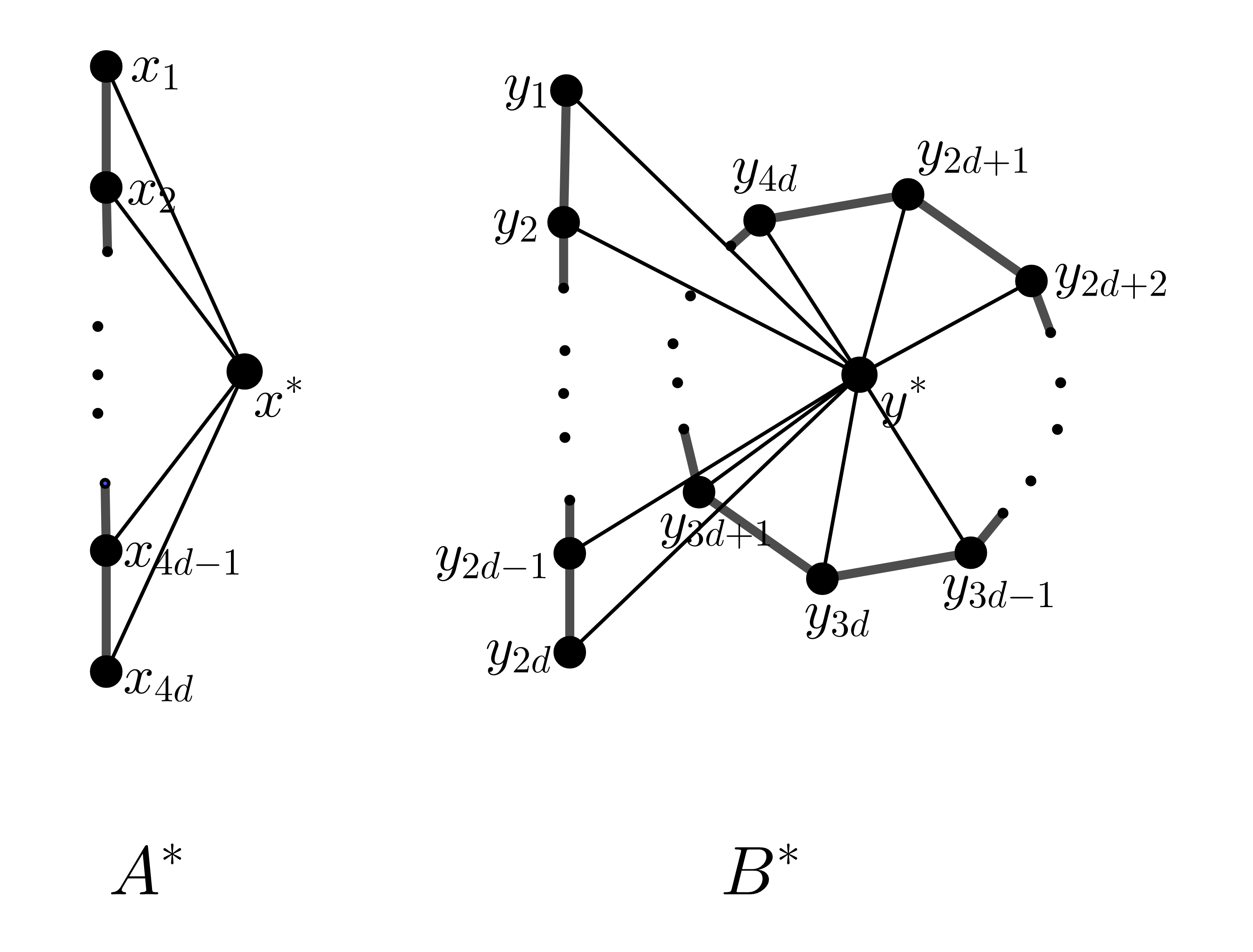
Figure 2. The graphs $A^{*}$ and $B^{*}$ for the query Chordal

Let $B_{1}$ and $B_{2}$ be the betweenness predicates of the graphs $A^{*}$ and $B^{*}$ and let $\mathbf{A}^{*}=(V_{1}^{*},B_{1})$ and $\mathbf{B}^{*}=(V_{2}^{*},B_{2})$ denote the graphic interval structures of $A^{*}$ and $B^{*}$. The edges of the graphs $A^{*}$ and $B^{*}$ are $E_{B_{1}}$ and $E_{B_{2}}$, respectively. Notice that both graphs $A^{*}$ and $B^{*}$ have diameter 2 and that $x^{*}$ (respectively, $y^{*}$) is contained in all intervals between two non-adjacent vertices $u,v$ of $A$ (respectively, of $B$). Consequently, for any vertices $u,v\in A$ (respectively, $u,v\in B$), we have $I(u,v)=\{u,v\}$ when $d_{A}(u,v)=1$ (respectively, $d_{B}(u,v)=1$), $I(u,v)=\{u,x^{*},v\}$ (respectively, $I(u,v)=\{u,y^{*},v\}$) if $d_{A}(u,v)\geq 3$ (respectively, $d_{B}(u,v)\geq 3$), and $I(u,v)=\{u,x^{*},z,v\}$ (respectively, $I(u,v)=\{u,y^{*},z,v\}$) if $d_{A}(u,v)=2$ (respectively, $d_{B}(u,v)=2$) and $z$ is the unique common neighbor of $u$ and $v$ in $A$ (respectively, in $B$). Using this structure of intervals in $A^{*}$ and $B^{*}$, we can establish the following result:

Claim 1.

Let $f$ be a partial map from $V_{1}^{*}$ to $V_{2}^{*}$ such that $f(x^{*})=y^{*}$ if $x^{*}$ is in the domain $X$ of $f$ or if $y^{*}$ is in the codomain $Y$ of $f$. If $f$ is an isomorphism between the subgraphs $H_{1}$ and $H_{2}$ induced by the sets $X$ and $Y$ in the graphs $A^{*}$ and $B^{*}$, respectively, then $f$ is a partial isomorphism between the interval structures $\mathbf{A}^{*}$ and $\mathbf{B}^{*}$.

Proof.

Since $f$ is an isomorphism from $H_{1}$ to $H_{2}$, observe that $f$ is necessarily injective. To establish the claim, we have to show that for any $u,v,z$ of $X$, we have $B_{1}(u,z,v)$ if and only if $B_{2}(f(u),f(z),f(v))$. This trivially holds if $u=v$ or if $z\in\{u,v\}$. Since $f$ is injective, this also holds if $f(u)=f(v)$ or if $f(z)\in\{f(u),f(v)\}$.

Thus suppose that $u\neq v$, $f(u)\neq f(v)$, $z\notin\{u,v\}$ and $f(z)\notin\{f(u),f(v)\}$. Since $f$ is an isomorphism from $H_{1}$ to $H_{2}$, we have that $u\sim v$ if and only if $f(u)\sim f(v)$. In this case, since $z\notin\{u,v\}$ and $f(z)\notin\{f(u),f(v)\}$, neither $B_{1}(u,z,v)$ nor $B_{2}(f(u),f(z),f(v))$ holds. Assume now that $u\nsim v$ and $f(u)\nsim f(v)$. Since $u$ and $v$ (respectively, $f(u)$ and $f(v)$) are at distance $2$ in $A^{*}$ (respectively, in $B^{*}$), we have $B_{1}(u,z,v)$ (respectively, $B_{2}(f(u),f(z),f(v))$) if and only if $z\sim u,v$ (respectively, $f(z)\sim f(u),f(v)$). Since $f$ is an isomorphism from $H_{1}$ to $H_{2}$, we have $z\sim u,v$ if and only if $f(z)\sim f(u),f(v)$ and consequently, $B_{1}(u,z,v)$ if and only if $B_{2}(f(u),f(z),f(v))$. This ends the proof of the claim. ∎

By Claim 1, to prove that the Duplicator wins the $r$-move EF-games on the interval structures ${\mathbf{A}}^{*}$ and ${\mathbf{B}}^{*}$ it sufficed to prove that the Duplicator wins the $r$-move EF-games on the graphs $A^{*}$ and $B^{*}$. We denote by $a_{i}$ and $b_{i}$ the vertices played in $A^{*}$ and $B^{*}$ at $i$th move of the game. Since $x^{*},y^{*},x_{1},x_{4d},y_{1},y_{2d}$ play a special role in the graphs $A^{*}$ and $B^{*}$ (they are the only vertices that are not of degree $4$), we set $a_{0}=x^{*}$, $b_{0}=y^{*}$, $a_{-1}=x_{1}$, $b_{-1}=y_{1}$, $a_{-2}=x_{4d}$, and $b_{-2}=y_{2d}$.

We describe a strategy for Duplicator to ensure that at any step $i$ of the game, the following conditions hold for all $-2\leq j\leq i$:

1. $a_{j}=a_{0}=x^{*}$ if and only if $b_{j}=b_{0}=y^{*}$,

2. if $a_{j}\neq x^{*}$, then there exists an isomorphism $f$ from the ball $B_{3^{r-i}}(a_{j},A)$ to the ball $B_{3^{r-i}}(b_{j},B)$ such that $f(a_{\ell})=b_{\ell}$ (respectively, $f^{-1}(b_{\ell})=a_{\ell}$) for any $a_{\ell}\in B_{3^{r-i}}(a_{j},A)$ (respectively, $b_{\ell}\in B_{3^{r-i}}(b_{j},B)$).

Observe that by our choice of $d$, when $a_{j}\neq x^{*}$ and $b_{j}\neq y^{*}$, the ball $B_{3^{r-i}}(a_{j},A)$ (respectively, $B_{3^{r-i}}(b_{j},B)$) is a path that is an isometric subgraph of $A$ (respectively, of $B$) for any $0\leq i\leq r$ and $-2\leq j\leq i$. Note also that condition (2) implies that:

1. if $x^{*}\notin\{a_{j},a_{\ell}\}$, then $d_{A}(a_{j},a_{\ell})>3^{r-i}$ if and only if $d_{B}(b_{j},b_{\ell})>3^{r-i}$,

2. if $x^{*}\notin\{a_{j},a_{\ell}\}$ and $d_{A}(a_{j},a_{\ell})\leq 3^{r-i}$, then $d_{A}(a_{j},a_{\ell})=d_{B}(b_{j},b_{\ell})$.

Before the start of the game, we have $i=0$ and the conditions (1) and (2) hold since $d_{A}(a_{-2},a_{-1})=4d-1\geq 4\cdot 3^{r+2}-1>3^{r}$ and $d_{B}(b_{-2},b_{-1})=2d-1\geq 2\cdot 3^{r+2}-1>3^{r}$. Assume now that conditions (1) and (2) hold for the first $i$ steps of the game and assume that the Spoiler picks $a_{i+1}\in A$ (the case where the Spoiler picks $b_{i+1}\in B$ is similar). First, suppose that $a_{i+1}=a_{j}$ for some $j\leq i$ (this holds in particular if $a_{i+1}\in\{x^{*},x_{1},x_{4d}\}$). In this case, set $b_{i+1}=b_{j}$ and observe that conditions (1) and (2) still hold after step $i+1$. Thus, further suppose that $a_{i+1}\neq a_{j}$ for any $j\leq i$. We distinguish two cases.

Case 1.

$d_{A}(a_{i+1},a_{j})>3^{r-(i+1)}$ for all $-2\leq j\leq i$ such that $a_{j}\neq x^{*}$.

For any $-2\leq j\leq i$ such that $b_{j}\in\{y_{1},\ldots,y_{d}\}$, the ball $B_{3^{r-(i+1)}}(b_{j},3^{r-(i+1)})$ contains at most $2\cdot 3^{r-(i+1)}+1$ vertices. Consequently, $\bigcup_{b_{j}\in\{y_{1},\ldots,y_{d}\}}B_{3^{r-(i+1)}}(b_{j},B)$ contains at most $(i+2)(2\cdot 3^{r-(i+1)}+1)$ vertices. Since $2d\geq 2\cdot 3^{r+2}>(i+2)(2\cdot 3^{r-(i+1)}+1)$, there exists a vertex $y_{k}$ with $1\leq k\leq 2d$ such that $y_{k}$ does not belong to any of these balls of radius $3^{r-(i+1)}$, i.e., for any $b_{j}$ such that $b_{j}\in\{y_{1},\ldots,y_{d}\}$, we have $d_{B}(y_{k},b_{j})>3^{r-(i+1)}$. Let Duplicator pick $b_{i+1}=y_{k}$ and observe that condition (1) is satisfied with this choice of $b_{i+1}$. We now show that condition (2) is also satisfied. For any $2\leq j\leq i$ such that $a_{j}\neq x^{*}$, we have $d_{A}(a_{i+1},a_{j})>3^{r-(i+1)}$ and $d_{B}(b_{i+1},b_{j})>3^{r-(i+1)}$. In particular, $d_{A}(a_{i+1},a_{-2})$, $d_{A}(a_{i+1},a_{-1})$, $d_{B}(b_{i+1},b_{-1})$, $d_{B}(b_{i+1},b_{-1})$ are greater than $3^{r-(i+1)}$ and thus the balls $B_{3^{r-(i+1)}}(a_{i+1},A)$ and $B_{3^{r-(i+1)}}(b_{i+1},B)$ are both paths of length $3^{r-i}$ that do not contain any vertex $a_{\ell}$ or $b_{\ell}$ with $\ell\leq i$, and thus condition (2) is satisfied for $a_{i+1}$. For all other vertices, condition (2) trivially holds by induction hypothesis.

Case 2.

There exists $-2\leq j\leq i$ such that $a_{j}\neq x^{*}$ and $d_{A}(a_{j},a_{i+1})\leq 3^{r-(i+1)}$.

By induction hypothesis, there is an isomorphism $f$ from the ball $B_{3^{r-i}}(a_{j},A)$ to the ball $B_{3^{r-i}}(b_{j},B)$ such that for any $a_{\ell}\in B_{3^{r-i}}(a_{j},A)$ (respectively, $b_{\ell}\in B_{3^{r-i}}(b_{j},B)$), we have $f(a_{\ell})=b_{\ell}$ (respectively, $f^{-1}(b_{\ell})=a_{\ell}$). Let Duplicator pick $b_{i+1}=f(a_{i+1})$ and note that condition (1) holds with such a choice. We now show that condition (2) also holds. Observe that for any $-2\leq\ell\leq i+1$ such that $a_{\ell}\in A$ and $a_{i+1}\in B_{3^{r-(i+1)}}(a_{\ell},A)$, the ball $B_{3^{r-(i+1)}}(a_{\ell},A)$ is included in $B_{3^{r-i}}(a_{j},A)$. Indeed, if $d_{A}(a_{\ell},a_{i+1})\leq 3^{r-(i+1)}$, we have $d_{A}(a_{\ell},a_{j})\leq d_{A}(a_{\ell},a_{i+1})+d_{A}(a_{i+1},a_{j})\leq 2\cdot 3^{r-(i+1)}$ and thus $B_{3^{r-(i+1)}}(a_{\ell},A)$ is included in $B_{3^{r-i}}(a_{\ell},A)$. Similarly, since $d_{B}(b_{i+1},b_{j})=d_{A}(a_{i+1},a_{j})\leq 3^{r-(i+1)}$, for any $-2\leq\ell\leq i+1$ such that $b_{\ell}\in B$ and $b_{i+1}\in B_{3^{r-(i+1)}}(b_{\ell},B)$, the ball $B_{3^{r-(i+1)}}(b_{\ell},B)$ is included in $B_{3^{r-i}}(b_{j},B)$. Therefore, $a_{i+1}\in B_{3^{r-(i+1)}}(a_{\ell},A)$ if and only if $b_{i+1}\in B_{3^{r-(i+1)}}(b_{\ell},B)$ and when it is the case, $f$ induces an isomorphism between the balls $B_{3^{r-(i+1)}}(a_{\ell},A)$ and $B_{3^{r-(i+1)}}(f(a_{\ell}),B)=B_{3^{r-(i+1)}}(b_{\ell},B)$. By induction hypothesis and since $f(a_{i+1})=b_{i+1}$, for any $-2\leq k\leq i+1$ such that $a_{k}\in B_{3^{r-(i+1)}}(a_{\ell},A)$ (respectively, $b_{k}\in B_{3^{r-(i+1)}}(b_{\ell},B)$), we have $f(a_{k})=b_{k}$ (respectively, $f^{-1}(b_{k})=a_{k}$). This establishes condition (2) for all balls containing $a_{i+1}$. For the other balls, the result holds trivially by induction hypothesis.

At the end of the game, i.e., after $r$ rounds, for any $-2\leq j,\ell\leq r$, we show that $a_{j}\sim a_{\ell}$ in $A^{*}$ if and only if $b_{j}\sim b_{\ell}$ in $B^{*}$. Note that by conditions (1) and (2), we have $a_{j}=a_{\ell}$ if and only if $b_{j}=b_{\ell}$. In this case, we have $a_{j}\nsim a_{\ell}$ and $b_{j}\nsim b_{\ell}$. Assume now that $a_{j}\neq a_{\ell}$ and $b_{j}\neq b_{\ell}$. If $a_{j}=x^{*}$ (respectively, $a_{\ell}=x^{*}$, $b_{j}=y^{*}$, $b_{\ell}=y^{*}$), then by condition (1), we have $b_{j}=y^{*}$ (respectively, $b_{\ell}=y^{*}$, $a_{j}=x^{*}$, $a_{\ell}=x^{*}$) and in this case we have $a_{j}\sim a_{\ell}$ and $b_{j}\sim b_{\ell}$ since $x^{*}$ and $y^{*}$ are respectively adjacent to all vertices of $A$ and $B$. Suppose now that $a_{j},a_{\ell}\in A$, $b_{j},b_{\ell}\in B$, and $a_{j}\sim a_{\ell}$ (respectively, $b_{j}\sim b_{\ell}$). By Condition (2), there is an isomorphism $f$ from $B_{1}(a_{j},A)$ to $B_{1}(b_{j},B)$ such that $f(a_{\ell})=b_{\ell}$ (respectively, $f^{-1}(b_{\ell})=a_{\ell})$. Consequently, $b_{\ell}=f(a_{\ell})\sim b_{j}=f(a_{j})$ (respectively, $a_{\ell}=f^{-1}(b_{\ell})\sim a_{j}=f^{-1}(b_{j})$ ) since $a_{\ell}\sim a_{j}$ (respectively, $b_{\ell}\sim b_{j}$).

Consequently, the map $f:a_{j}\mapsto b_{j}$ defines an isomorphism between the graphs induced by $X=\{a_{-2},a_{-1},\ldots,a_{r}\}$ in $A^{*}$ and $Y=\{b_{-2},b_{-1},\ldots,b_{r}\}$ in $B^{*}$. By Claim 1, we get that the Duplicator wins the $r$-moves EF-game on the interval structure ${\mathbf{A}}^{*}=(V_{1}^{*},B_{1})$ and ${\mathbf{B}}^{*}=(V_{2}^{*},B_{2})$. By Theorem 3, Chordal is not FOLB-definable.

To the query Dismantlable. We consider the same graphs $A=(V_{1},E_{1})$ and $B=(V_{2},E_{2})$ as in query Chordal. Let $A^{*}$ be the graph obtained by adding two non-adjacent vertices $x^{*}_{1}$ and $x^{*}_{2}$ and making them adjacent to all vertices in $A$ and let $B^{*}$ be the graph obtained by adding two non-adjacent vertices $y^{*}_{1}$ and $y^{*}_{2}$ and making them adjacent to all vertices of $B$; see Fig. 3. Then $x_{1},x_{2},\ldots,x_{4d-1},x^{*}_{1},x^{*}_{2},x_{4d}$ is a dismantling order of $A^{*}$ because each vertex $x_{i},i<4d$ is dominated in the subgraph induced by the remaining vertices by the vertex $x_{i+1}$ while the subgraph induced by the last three vertices $x^{*}_{1},x^{*}_{2},x_{4d}$ is a 2-path with $x_{4d}$ as the middle vertex. On the other hand, the graph $B^{*}$ is not dismantlable because the unique way to partially dismantle $B^{*}$ is to remove the vertices of the path of $B_{r}$ either in order $y_{1},y_{2},\ldots,y_{2d}$ or in the reverse order $y_{2d},y_{2d-1}\ldots,y_{1}$. The resulting subgraph of $B^{*}$ is a double wheel induced by the cycle $(y_{2d+1},\ldots,y_{4d})$ and two non-adjacent vertices $y_{1}^{*}$ and $y^{*}_{2}$ and this subgraph does not contain any dominated vertex.

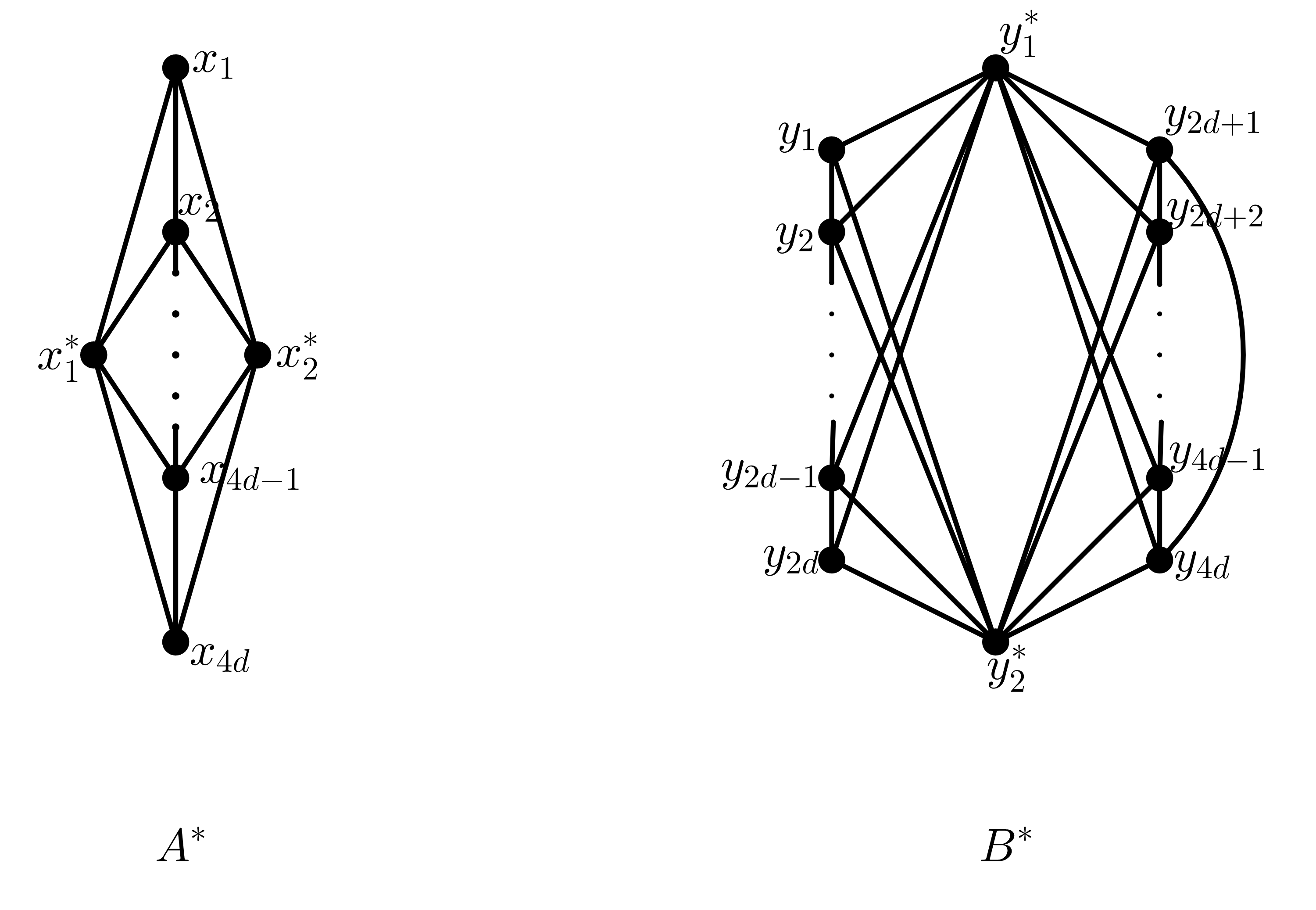
Figure 3. The graphs $A^{*}$ and $B^{*}$ for the query Dismantlable

Let $B_{1}$ and $B_{2}$ be the betweenness predicates of the graphs $A^{*}$ and $B^{*}$. Let ${\mathbf{A}}^{*}=(V_{1}^{*},B_{1})$ and $\mathbf{B}^{*}=(V_{2}^{*},B_{2})$, where $V_{1}^{*}=V_{1}\cup\{x^{*}_{1},x^{*}_{2}\}$ and $V_{2}^{*}=V_{2}\cup\{y^{*}_{1},y^{*}_{2}\}$. Note that both graphs $A^{*}$ and $B^{*}$ have diameter 2 and that $x_{1}^{*},x_{2}^{*}$ (respectively, $y_{1}^{*},y_{2}^{*}$) are contained in all intervals between non-adjacent vertices $u,v$ of $A$ (respectively, of $B$). Consequently, for any vertices $u,v\in A$ (respectively, $u,v\in B$), we have $I(u,v)=\{u,v\}$ when $d_{A}(u,v)=1$ (respectively, $d_{B}(u,v)=1$), $I(u,v)=\{u,x_{1}^{*},x_{2}^{*},v\}$ (respectively, $I(u,v)=\{u,y_{1}^{*},y_{2}^{*},v\}$) if $d_{A}(u,v)\geq 3$ (respectively, $d_{B}(u,v)\geq 3$), and $I(u,v)=\{u,x_{1}^{*},x_{2}^{*},z,v\}$ (respectively, $I(u,v)=\{u,y_{1}^{*},y_{2}^{*},z,v\}$) if $d_{A}(u,v)=2$ (respectively, $d_{B}(u,v)=2$) and $z$ is the unique common neighbor of $u$ and $v$ in $A$ (respectively, in $B$). Observe also that $I(x_{1}^{*},x_{2}^{*})=V(A^{*})$ and $I(y_{1}^{*},y_{2}^{*})=V(B^{*})$.

Using this structure of intervals and a proof similar to the proof of Claim 1, one can establish that for any map $f$ from $X\subseteq V_{1}^{*}$ to $Y\subseteq V_{2}^{*}$ such that $f(x_{1}^{*})=y_{1}^{*}$ if $x_{1}^{*}\in X$ or $y_{1}^{*}\in Y$, $f(x_{2}^{*})=y_{2}^{*}$ if $x_{2}^{*}\in X$ or $y_{2}^{*}\in Y$, if $f$ is an isomorphism between the subgraphs induced by $X$ and $Y$ in the graphs $A^{*}$ and $B^{*}$, then $f$ is a partial isomorphism between the interval structures $A^{*}$ and $B^{*}$. Then, using a proof similar as in the case of chordal graphs, we can establish that Duplicator wins the EF-games on $\mathbf{A}^{*}$ and $\mathbf{B}^{*}$. By Theorem 3, this implies that Dismantlable is not FOLB-definable.

To the query Planar. We consider the same graphs $A=(V_{1},E_{1})$ and $B=(V_{2},E_{2})$ as in queries Chordal and Dismantlable and the same graphs $A^{*}$ and $B^{*}$ in the query Dismantlable. The graph $A^{*}$ is planar: a planar drawing of $A^{*}$ is given in Fig. 3. On the other hand, $B^{*}$ is not planar because it contains $K_{5}$ as a minor. This $K_{5}$-minor is defined by any three distinct vertices $y_{i},y_{j},y_{k}$ of the cycle $C$ of $B$ and the vertices $y^{*}_{1},y^{*}_{2}$. The vertices $y_{i},y_{j},y_{k}$ are connected by three disjoint subpaths of the cycle $C$, $y^{*}_{1}$ and $y^{*}_{2}$ are connected to $y_{i},y_{j},y_{k}$ by edges, and $y_{1}^{*}$ and $y^{*}_{2}$ are connected by a path of length 2 passing via the path of $B$. The result then follows from the fact that the Duplicator wins the EF-game on $\mathbf{A}^{*}$ and $\mathbf{B}^{*}$.

To the query Partial Johnson. Consider the graphs $A=(V_{1},E_{1})$ and $B=(V_{2},E_{2})$, where $A$ is a cycle $(x_{1},x_{2},\ldots,x_{2d-1},x_{2d},x_{1})$ with $2d$ vertices and $B$ consists of two odd cycles $(y_{1},y_{2},\ldots,y_{d-1},y_{d})$ and $(y_{d+1},\ldots,y_{2d},y_{d+1})$. Let $A^{*}$ be the graph obtained by adding a vertex $x^{*}$ and making it adjacent to all vertices of $A$ and let $B^{*}$ be the graph obtained by adding a vertex $y^{*}$ and making it adjacent to all vertices in $B$. One can directly check (or use the result of [72]) that $A^{*}$ is a partial Johnson graph and $B^{*}$ is not a partial Johnson graph because $B^{*}$ contains odd wheels. Since the structure of intervals in this pairs of graphs is similar to the graphs considered in the case of the query Chordal, an analogous of Claim 1 for this pair of graphs also holds. Then, using the same proof as in the case of chordal graphs (where the vertices $a_{-2},a_{-1},b_{-2},b_{-1}$ are not defined), we can establish that Duplicator wins the EF-games on $\mathbf{A}^{*}$ and $\mathbf{B}^{*}$. By Theorem 3, this implies that Dismantlable is not FOLB-definable.

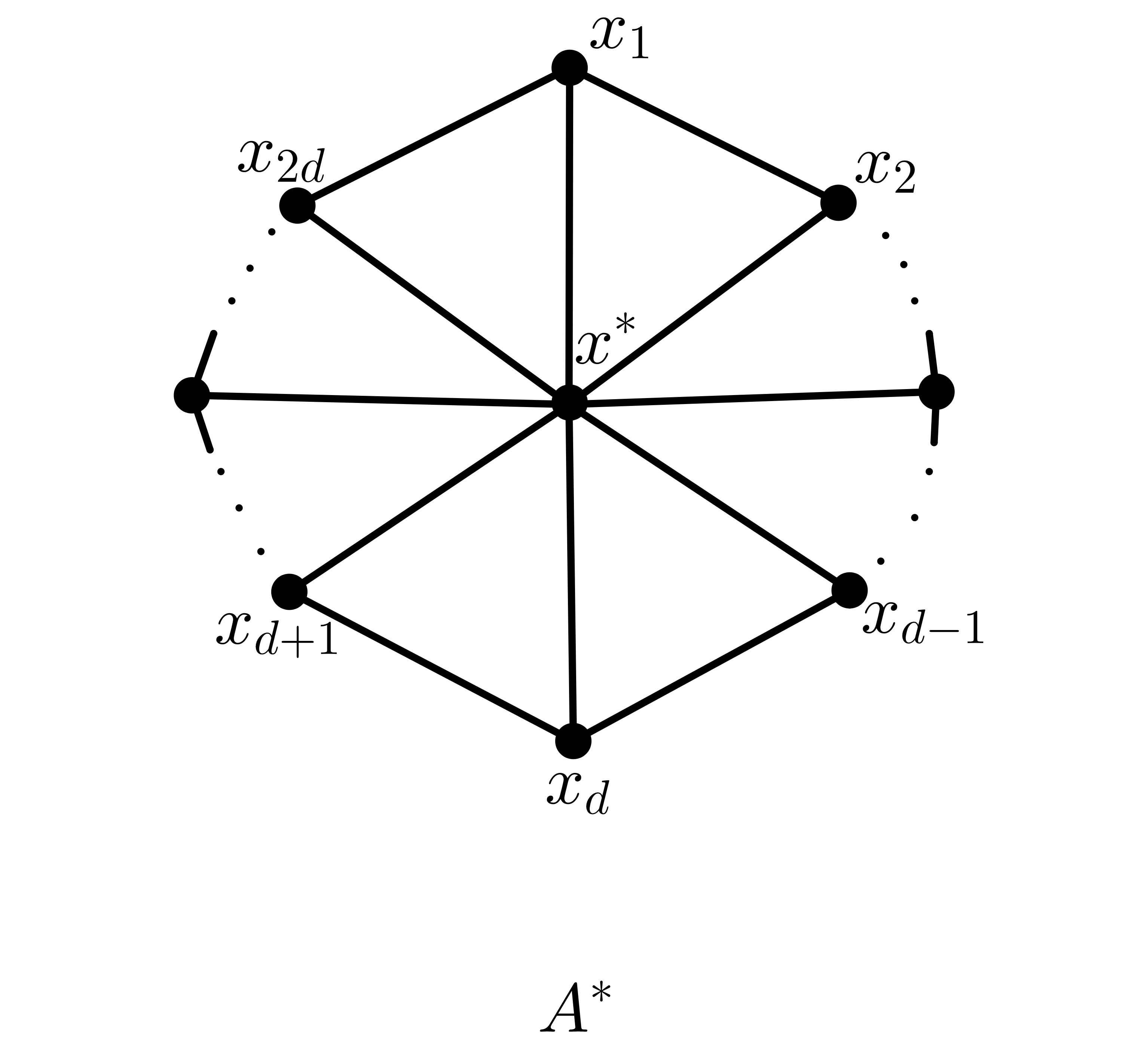
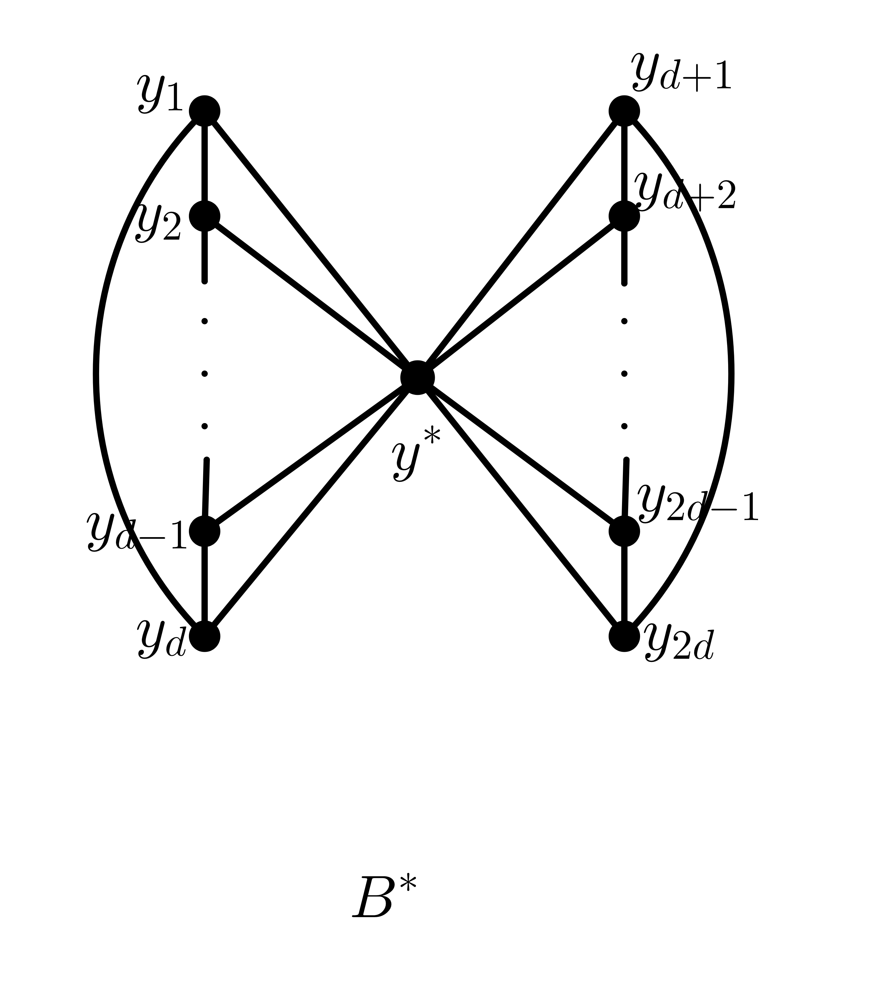
Figure 4. The graphs $A^{*}$ and $B^{*}$ for the query Partial Johnson

To the query Eulerian. For any $r\geq 1$, consider the graphs $A=(V_{1},E_{1})$ and $B=(V_{2},E_{2})$, where $A=\overline{K}_{2r}$ is a stable set of size $2r$ and $B=\overline{K}_{2r+1}$ is a stable set of size $2r+1$. Let $A^{*}$ be the graph obtained by adding two non-adjacent vertices $x^{*}_{1}$ and $x^{*}_{2}$ and making them adjacent to all vertices in $A_{r}$ and let $B^{*}$ be the graph obtained by adding two non-adjacent vertices $y^{*}_{1}$ and $y^{*}_{2}$ and making them adjacent to all vertices of $B_{r}$. Clearly, $A^{*}$ and $B^{*}$ are the complete bipartite graphs $K_{2,2r}$ and $K_{2,2r+1}$. Let $V_{1}=\{x_{1},\ldots,x_{2r}\},V_{2}=\{y_{1},\ldots,y_{2r},y_{2r+1}\}$ and $V_{1}^{*}=V_{1}\cup\{x^{*}_{1},x^{*}_{2}\},V_{2}^{*}=V_{2}\cup\{y^{*}_{1},y^{*}_{2}\}$. Obviously, $A^{*}$ is an Eulerian graph and $B^{*}$ is not Eulerian. Let $B_{1}$ and $B_{2}$ be the betweenness predicates of the graphs $A^{*}$ and $B^{*}$ and consider the interval structures $\mathbf{A}^{*}=(V_{1}^{*},B_{1})$ and $\mathbf{B}^{*}=(V_{2}^{*},B_{2})$. Both graphs $A^{*}$ and $B^{*}$ have diameter 2 and one easily see that for any two vertices $u,v$ of $A$ (respectively, $B$), we have $I(u,v)=\{u,x^{*}_{1},x^{*}_{2},v\}$ (respectively, $I(u,v)=\{u,y^{*}_{1},y^{*}_{2},v\}$). Observe also that $I(x_{1}^{*},x_{2}^{*})=V_{1}^{*}$ and $I(y_{1}^{*},y_{2}^{*})=V_{2}^{*}$.

Using this structure of intervals and a proof similar (but simpler) to the proof of Claim 1, one can establish that for any map $f$ from $X\subseteq V_{1}^{*}$ to $Y\subseteq V_{2}^{*}$ such that $f(x_{1}^{*})=y_{1}^{*}$ if $x_{1}^{*}\in X$ or $y_{1}^{*}\in Y$, $f(x_{2}^{*})=y_{2}^{*}$ if $x_{2}^{*}\in X$ or $y_{2}^{*}\in Y$, if $f$ is an isomorphism between the subgraphs induced by $X$ and $Y$ in the graphs $A^{*}$ and $B^{*}$, then $f$ is a partial isomorphism between the interval structures $A^{*}$ and $B^{*}$. Then, using a proof similar as in the case of chordal graphs, we can establish that Duplicator wins the EF-games on $\mathbf{A}^{*}$ and $\mathbf{B}^{*}$. By Theorem 3, this implies that Eulerian is not FOLB-definable. ∎

Since FOLB-queries can be tested in polynomial time on any graph $G$ (see Section 8), any property that is NP-hard to recognize is unlikely to be expressible as a FOLB-query. It is known that it is NP-complete to decide whether a given graph admits a distance preserving order [76]. Therefore if P$\neq$NP, DPO cannot be expressed as a FOLB-query. In fact, one can show that DPO is not expressible as a FOLB-query. To establish this result, one can proceed as in the proof of Proposition 1 in order to prove that Duplicator wins the games on the two graphs $A^{*}$ and $B^{*}$ from Figure 5 ($A^{*}$ has a distance preserving order while $B^{*}$ does not). Since these graphs have diameter 4, in order to give a formal proof, we need to adapt Claim 1 and the inductive condictions (1) and (2) used in the proof of Proposition 1. Notice that in these graphs, we have nine different types of intervals. We do not give a proof of this result, because this would need a lengthy proof leading to an expected conclusion.

Figure 5. The graphs $A^{*}$ and $B^{*}$ for the query DPO

8. Running time of FOLB queries

Let $\phi$ be an FO sentence in vocabulary $\sigma$, and let $\mathbf{A}$ be a $\sigma$-structure. Encoding of a formula $\phi$, $enc(\phi)$, could be its syntactic tree represented as a string. The length of this string, $enc(\phi)$, is denoted by $||\phi||$. We define the encoding $enc(\mathbf{A})$ of a structure $\mathbf{A}$ as the concatenation of $0^{n}1$ and all the $enc(R_{i})$, where $n$ is the cardinality of the domain of $\mathbf{A}$ and $R_{i}$, for each $i=1,2,\ldots,l$ is the relation symbol in the signature of $\mathbf{A}$. That is, $enc(\mathbf{A})=0^{n}1.enc(R_{1})\cdots enc(R_{l})$. The length of this string is $||\mathbf{A}||=(n+1)+\sum_{i=1}^{p}n^{arity(R_{i})}$. The width of an FO formula $\phi$ is the maximum number of free variables in a subformula of $\phi$. The running time of FO queries in terms of the size of encodings of a FO query and a structure is given in [118] as follows:

Proposition 2 (​​[118]).

Let $\phi$ be an FO sentence in vocabulary $\sigma$ and let $\mathbf{A}$ be a $\sigma$-structure. If the width of $\phi$ is $k$, then checking whether $\mathbf{A}$ is a model of $\phi$ can be done in time $O(||\phi||\times||\mathbf{A}||^{k})$.

This gives a polynomial time algorithm for evaluating FO queries on finite structures, for a fixed sentence $\phi$.

The interval structure $\mathbf{G}=(V,B)$ with $|V|=n$ and $B$, being a ternary relation, can be encoded by a string of length $||\mathbf{G}||=(n+1+n^{3})$. Furthermore, for the fixed formula $\phi$, the $||\phi||$ is a constant, say $c$. The total number of variables used in $\phi$ will be the upper bound for $k$. Note that every FOLB sentence defined in this paper uses a fixed number of variables and, in some cases, the subformulas given by the query $\operatorname*{\sf Subgraph}$ or $\operatorname*{\sf Isometric}$ in sentence $\phi$ maximum contributes to the width of $\phi$. Thus for a fixed sentence $\phi$ in FOLB, checking whether $\mathbf{A}$ is a model of $\phi$ can be done in time $O(||\phi||\times||\mathbf{A}||^{k})$ $=$ $O(c\times(n+1+n^{3})^{k})=O(c\times n^{3k})$. Note that a particular FOLB-query for a graph class $\mathcal{C}$ actually characterizes $\mathcal{C}$. The recognition of a graph class $\mathcal{C}$ is defined as the decision problem “does a given graph $G$ belong the graph class $\mathcal{C}$?". The input is an arbitrary graph $G$ and the output is True if and only if $G$ belongs to $\mathcal{C}$ and False otherwise. If there is a corresponding FOLB-query characterising the graph class $\mathcal{C}$, then for a given graph $G$, we can ensure that there exists an algorithm to check whether $G$ is in the graph class $\mathcal{C}$ using that FOLB query. From all these observations we obtain the following remark:

Proposition 3.

All FOLB-definable graph classes given in Theorem 10 can be recognized in polynomial time.

Notice that most of the classes of graphs from Theorem 10 can be recognized by more efficient algorithms than those using Propositions 2 and 3.

9. Conclusion

In this paper, we showed that most of graph classes investigated in Metric Graph Theory are definable in FOLB. On the other hand, we showed that several sub- or super-classes of them are not definable in FOLB. Tarski’s theory uses the predicates “betweenness” and “congruence”. For graphs, the congruence is the quaternary relation $\equiv$ meaning that $uv\equiv u^{\prime}v^{\prime}$ if $d(u,v)=d(u^{\prime},v^{\prime})$ and we can call the resulting logic the Fist Order Logic with Betweenness and Congruency, abbreviated FOLBC. However, for graphs it seems that FOLBC is not more expressible than FOLB. At least the graph classes not expressible in FOLB remains not expressible in FOLBC and for all classes for which FOLB-definability is open the FOLBC-definability is open as well. On the other hand, if instead of the congruency axiom one can compute distances between vertices of a graph, then the property “the hyperbolicity of a graph is at most $\delta$” becomes easily expressible. Distance computation and angle measurement (Scale and Protractor) is at the basis of classical metric approach to plane geometry due to Birkhoff [31] (see the book [123]). Note that FOLB can be extended to disconnected graphs [55]. Another perspective is to consider the Monadic Second Order Logic with Betweenness for graphs. Finally, an important long term research perspective is the algorithmic status of FOLB model checking on FOLB-definable classes of graphs: : for a FOLB-definable class $\mathcal{C}$, can we find an algorithm that given a FOLB formula $\phi$ and a graph $G\in\mathcal{C}$ on $n$ vertices check whether $G$ satisfies $\phi$ in time $f(\phi)\cdot\operatorname{poly}(n)$ where the polynomial in $n$ is independent of $\phi$.

References

- [1] M. Albenque and K. Knauer, Convexity in partial cubes: the hull number, Discr. Math. 339 (2016), 866–876.
- [2] R. P. Anstee and M. Farber, On bridged graphs and cop-win graphs, J. Combin. Theory Ser. B 44 (1988), no. 1, 22–28.
- [3] T. Aougab, Uniform hyperbolicity of the graphs of curves, Geom. Topol. 17 (2013), 2855–-2875.
- [4] S. P. Avann, Metric ternary distributive semi-lattices. Proc. Amer. Math. Soc., 12 (1961) 407–414.
- [5] K. Balakrishnan, M. Changat, A.K. Lakshmikuttyamma, J. Mathew, H.M. Mulder, P.G. Narasimha-Shenoi, and N. Narayanan, N., Axiomatic characterization of the interval function of a block graph. Discr. Math., 338 (2015), 885–894.
- [6] H.-J. Bandelt, Characterizing median graphs, manuscript (1982).
- [7] H.-J. Bandelt, Retracts of hypercubes, J. Graph Th., 8 (1984), 501–510.
- [8] H.-J. Bandelt, Graphs with intrinsic convexities, J. Graph Th., 13 (1989), 215–228.
- [9] H.-J. Bandelt and V. Chepoi, A Helly theorem in weakly modular space, Discr. Math. 160 (1996), 25–39.
- [10] H.-J. Bandelt and V. Chepoi, Cellular bipartite graphs, Europ. J. Combin. 17 (1996), 121–134.
- [11] H.-J. Bandelt and V. Chepoi, Decomposition and -embedding of weakly median graphs, Europ. J. Combin. 21 (2000), 701–714.
- [12] H.-J. Bandelt and V. Chepoi, Graphs with connected medians, SIAM J. Discr. Math. 16 (2002), 268–282.
- [13] H.-J. Bandelt, V. Chepoi, 1-Hyperbolic graphs, SIAM J. Discr. Math. 16 (2003) 323–334.
- [14] H.-J. Bandelt and V. Chepoi, Metric graph theory and geometry: a survey, Surveys on Discrete and Computational Geometry: Twenty Years Later, J.E. Goodman, J. Pach, and R. Pollack (eds), Contemp. Math., 453 (2008), pp. 49–86.
- [15] H.-J. Bandelt, V. Chepoi, A. Dress, and J. Koolen, Combinatorics of lopsided sets, Eur. J. Comb. 27 (2006), 669–689.
- [16] H.-J. Bandelt, V. Chepoi, and K. Knauer, COMs: complexes of oriented matroids, J. Combin. Th., Ser. A 156 (2018), 195–237.
- [17] H.-J. Bandelt, V. Chepoi, and M. van de Vel, Pasch-Peano spaces and graphs, preprint, 1993.
- [18] H.-J. Bandelt and A.W.M. Dress, A canonical decomposition theory for metrics on a finite set, Adv. Math. 92 (1992), 47–105.
- [19] H.-J. Bandelt and H.M. Mulder, Distance-hereditary graphs, J. Combin. Th. Ser. B 41 (1986), 182–208.
- [20] H.-J. Bandelt and H. M. Mulder, Infinite median graphs, (0,2)-graphs, and hypercubes, J. Graph Theory 7 (1983), 487–497.
- [21] H.-J. Bandelt and H.M. Mulder, Pseudo-modular graphs, Discr. Math. 62 (1986), 245–260.
- [22] H.-J. Bandelt and H.M. Mulder, Pseudo-median graphs are join spaces, Discr. Math. 109 (1992), 13-26.
- [23] H.-J. Bandelt, H.M. Mulder, and E. Wilkeit, Quasi-median graphs and algebras, J. Graph Th. 18 (1994), 681–703.
- [24] H.-J. Bandelt, P. Forster, and A. Röhl, Median-joining networks for inferring intraspecic phylogenies, Mol. Biol. Evol. 16 (199), 37–48.
- [25] H.-J. Bandelt and E. Pesch, Dismantling absolute retracts of reflexive graphs, European J. Combin. 10 (1989), no. 3, 211–220.
- [26] H.-J. Bandelt and E. Prisner, Clique graphs and Helly graphs, J. Combin. Theory Ser. B 51 (1991), no. 1, 34–45,
- [27] H.-J. Bandelt, M. van de Vel, and E. Verheul, Modular interval spaces, Math. Nachr. 163 (1993), 177–201.
- [28] J.-P. Barthélémy and J. Constantin, Median graphs, parallelism and posets, Discrete Math. 111 (1993), no. 1-3, 49–63.
- [29] L.W. Beineke, Characterizations of derived graphs, J. Combin. Th. Ser B, 9 (1970), 129–135.
- [30] C. Berge and P. Duchet, A generalization of Gilmore’s theorem, Recent advances in graph theory (Proc. Second Czechoslovak Sympos., Prague, 1974), 1975, pp. 49–55.
- [31] G.D. Birkhoff, A set of postulates for plane geometry, based on scale and protractor, Annals of Math., 33 (1932), 329–345.
- [32] G. Birkhoff and S. A. Kiss, A ternary operation in distributive lattices, Bull. Amer. Math. Soc., 53 (1947) 749–752.
- [33] R. Bland and M. Las Vergnas, Orientability of matroids, J. Combin. Th. Ser. B, 23 (1978), 94–123.
- [34] A. Björner, P. H. Edelman, and G. M. Ziegler, Hyperplane arrangements with a lattice of regions, Discr. Comput. Geom., 5 (1990), pp. 263–288.
- [35] A. Björner, M. Las Vergnas, B. Sturmfels, N. White, and G. Ziegler, Oriented Matroids, Encyclopedia of Mathematics and its Applications, vol. 46, Cambridge University Press, Cambridge, 1993.
- [36] B. Bollobás and A.J. Radcliffe, Defect Sauer results, J. Comb. Th. Ser. A 72 (1995), 189–208.
- [37] B. Brešar, Characterizing almost-median graphs, Eur. J. Combin., 28 (2007), 916–920.
- [38] B. Brešar, J. Chalopin, V. Chepoi, T. Gologranc, and D. Osajda, Bucolic complexes, Adv. Math. 243 (2013), 127–167.
- [39] M. R. Bridson and A. Haefliger, Metric spaces of non-positive curvature, Grundlehren der Mathematischen Wissenschaften [Fundamental Principles of Mathematical Sciences], vol. 319, Springer-Verlag, Berlin, 1999.
- [40] A. E. Brouwer and A. M. Cohen, Local recognition of Tits geometries of classical type, Geom. Dedicata 20 (1986), no. 2, 181–19
- [41] L.M. Blumenthal, Theory and Applications of Distance Geometry, Oxford University Press, 1953.
- [42] A.V. Borovik, I.M. Gelfand, and N. White, Coxeter Matroids, Progr. Math., vol. 216, Birkhäuser, Boston, 2003.
- [43] A. Bouchet, Greedy algorithm and symmetric matroids, Math. Program. 38 (1987) 147–159.
- [44] B.H. Bowditch, Intersection numbers and the hyperbolicity of the curve complex, J. Reine Angew. Math. 598 (2006), 105–-129.
- [45] J. Calder, Some elementary properties of interval convexities, J. London Math. Soc. 3 (1971), 422–428.
- [46] P. J. Cameron, Dual polar spaces, Geom. Dedicata 12 (1982), no. 1, 75–85.
- [47] J. Chalopin, V. Chepoi, and D. Osajda, On two conjectures of Maurer concerning basis graphs of matroids, J. Combin. Theory Ser. B 114 (2015), 1–32.
- [48] J. Chalopin and V. Chepoi, A counterexample to Thiagarajan’s conjecture, J. Comput. Syst. Sci. 113 (2020), 76–100.
- [49] J. Chalopin and V. Chepoi, 1-Safe Petri nets and special cube complexes: equivalence and applications, ACM Transactions on Computational Logic, Vol. 20, No. 3, Article 17, 49 pages.
- [50] J. Chalopin, V. Chepoi, and H. Hirai, and D. Osajda, Weakly modular graphs and nonpositive curvature, Memoirs of AMS, 268 (2020), no. 1309.
- [51] J. Chalopin, V. Chepoi, H. Hirai, A. Genevois, and D. Osajda, Helly groups.
- [52] J. Chalopin, V. Chepoi, S. Moran, and M. Warmuth, Unlabeled sample compression schemes and corner peelings for ample and maximum classes, J. Comput. Syst. Sci, 127 (2022), 1–28.
- [53] J. Chalopin, V. Chepoi, and U. Giocanti, Graphs with convex balls.
- [54] R. Chandrasekaran and S.N. Kabadi, Pseudomatroids, Discrete Math. 71 (1988) 205–217.
- [55] M. Changat, F.H. Nezhad, H.M. Mulder, and N. Narayanan, A note on the interval function of a disconnected graph, Discussiones Mathematicae Graph Theory, 38 (2018), 39–48.
- [56] M. Changat, H.M. Ferdoos, and N. Narayanan, Axiomatic characterization of the interval function of a bipartite graph, Discrete Applied Mathematics 286 (2020): 19-28.
- [57] M. Changat, P.G. Narasimha-Shenoi, and G. Seethakuttyamma, Betweenness in graphs: a short survey on shortest and induced path betweenness, AKCE International Journal of Graphs and Combinatorics (2018).
- [58] Changat M, Lakshmikuttyamma AK, Mathews J, Peterin I, Narasimha-Shenoi PG, Seethakuttyamma G, and Špacapan S., A forbidden subgraph characterization of some graph classes using betweenness axioms, Discr. Math. 313 (2013), 951-8.
- [59] Changat M., Sheela LK, Narasimha-Shenoi PG, The interval function, Ptolemaic, distance hereditary, bridged graphs and axiomatic characterizations, arXiv preprint arXiv:2005.06751. 2020.
- [60] V.D. Chepoi, Some properties of domain finite convexity structures (in Russian), Res. Algebra, Geometry and Appl. (Moldova State University) (1986), 142–148.
- [61] V. Chepoi, Geometric properties of -convexity in bipartite graphs, Modelironvanie Informacionnych Sistem (Chişinău, Stiinţa), 1986, 88–100.
- [62] V. Chepoi, Some properties of -convexity in triangulated graphs, Mat. Issled., 87, (Chişinău, Stiinţa), 1986, 164–177.
- [63] V. Chepoi, -Convex sets in graphs, Dissertation, Moldova State Univ., Chişinău, 1986.
- [64] V. Chepoi, Classifying graphs by metric triangles, Metody Diskretnogo Analiza 49 (1989), 75–93 (Russian).
- [65] V. Chepoi, Isometric subgraphs of Hamming graphs and -convexity, Cybernetics 24 (1988), 6–10.
- [66] V. Chepoi, Separation of two convex sets in convexity structures, J. Geometry 50 (1994), 30–51.
- [67] V. Chepoi, Bridged graphs are cop-win graphs: an algorithmic proof, J. Combin. Theory Ser. B 69 (1997), no. 1, 97–100.
- [68] V. Chepoi, On distance-preserving and domination elimination orderings, SIAM J. Discrete Math. 11 (1998), no. 3, 414–436.
- [69] V. Chepoi, Graphs of some CAT(0) complexes, Adv. Appl. Math. 24 (2000), 125–179.
- [70] V. Chepoi, Basis graphs of even delta-matroids, J. Combin. Th. Ser. B. 97 (2007), no. 2, 175–192
- [71] V. Chepoi, Nice labeling problem for event structures: a counterexample, SIAM J. Comput. 41 (2012), 715–-727.
- [72] V. Chepoi, Distance-preserving subgraphs of Johnson graphs, Combinatorica 37 (2017), 1039–1055.
- [73] V. Chepoi, F. Dragan, B. Estellon, M. Habib, and Y. Vaxès, Diameters, centers, and approximating trees of delta-hyperbolic geodesic spaces and graphs, Symposium on Computational Geometry, SoCG’2008, pp.59–68.
- [74] V. Chepoi, K. Knauer, and T. Marc, Hypercellular graphs: Partial cubes without as partial cube minor, Discr. Math. 343 (2020), 111678.
- [75] V. Chepoi and D. Osajda, Dismantlability of weakly systolic complexes and applications, Trans. Amer. Math. Soc. 367 (2015), no. 2, 1247–1272.
- [76] D. Coudert, G. Ducoffe, N. Nisse, and M. Soto, On distance-preserving elimination orderings in graphs: complexity and algorithms, Discret. Appl. Math. 243 (2018), 140–153.
- [77] I. da Silva, Axioms for maximal vectors of an oriented matroid: a combinatorial characterization of the regions determined by an arrangement of pseudohyperplanes, Eur. J. Comb., 16 (1995), 125–145.
- [78] M. W. Davis, The geometry and topology of Coxeter groups, vol. 32 of London Mathematical Society Monographs Series, Princeton University Press, 2008.
- [79] P. Deligne, Les immeubles des groupes de tresses généralisés, Inventiones mathematicae 17 (1972), 273–302.
- [80] M. Deza and M. Laurent, Geometry of Cuts and Metrics, Springer-Verlag, Berlin, 1997.
- [81] D.Ž. Djoković, Distance–preserving subgraphs of hypercubes, J. Comb. Th. Ser. B 14 (1973), 263–267.
- [82] F. F. Dragan, Centers of graphs and the Helly property (in Russian), Chişinău, Republica Moldova, 1988.
- [83] F.F. Dragan and H. M. Guarnera, Obstructions to a small hyperbolicity in Helly graphs, Discrete Math. 342 (2019), no. 2, 326–338.
- [84] A. W. M. Dress, Trees, tight extensions of metric spaces, and the cohomological dimension of certain groups: a note on combinatorial properties of metric spaces, Adv. in Math. 53 (1984), no. 3, 321–402.
- [85] A.W.M. Dress, T. Havel, Some combinatorial properties of discriminants in metric vector spaces, Adv. Math. 62 (1986) 285–312.
- [86] P.H. Edelman and R.E. Jamison, The theory of convex geometries, Geom. Dedicata 19 (1985), 247–270.
- [87] A. Ehrenfeucht, An application of games to the completeness problem for formalized theories, Fund. Math., 49 (1961), 129–-141.
- [88] J.E. Ellis, A general set-separation theorem, Duke Math. J. 19 (1952) 417–421.
- [89] J. Folkman and J. Lawrence, Oriented matroids, J. Combin. Th. Ser. B, 25 (1978), 199–236.
- [90] R. Fraïssé, Sur quelques classifications des syst‘emes de relations, Publ. Sci. Univ. Alger. Sér. A, 1 (1954), 35–-182.
- [91] M. Farber and R. E. Jamison, On local convexity in graphs, Discrete Math. 66 (1987), no. 3, 231–247.
- [92] A. Genevois, Cubical-like geometry of quasi-median graphs and applications to geometric group theory. PhD thesis, arxiv:1712.01618, 2017.
- [93] E. Ghys, A.H. Haefliger, A. Verjovsky (eds.), Group Theory from a Geometric Viewpoint, World Scientific, Singapore, 1991.
- [94] M.C. Golumbic, Algorthmic graph theory and perfect graphs, 2nd Edition, Ann. Discr. Math. 57, 2004.
- [95] M. Gromov, Hyperbolic groups, Essays in group theory, Math. Sci. Res. Inst. Publ., vol. 8, Springer, New York, 1987, pp. 75–263.
- [96] R. L. Graham et H. O. Pollak, On the addressing problem for loop switching, The Bell System Technical Journal 50 (1971), p. 2495–2519.
- [97] M.F. Hagen, Weak hyperbolicity of cube complexes and quasi-arboreal groups. J. Topol. 7 (2014), 385–418.
- [98] F. Haglund and F. Paulin, Simplicité de groupes d’automorphismes d’espaces à courbure négative, The Epstein birthday schrift, Geom. Topol. Monogr., 1 (1998), 181–248. Geom. Topol. Publ., Coventry.
- [99] R. Hammack, W. Imrich, and S. Klavz̆ar, Handbook of Product Graphs, Discrete Math. Appl. CRC press, Boca Raton, 2nd edition, 2011.
- [100] J. Hedlíková, Ternary spaces, media, and Chebyshev sets, Czechoslovak Math. J. 33 (1983), 373–389.
- [101] S. Hensel, P. Przytycki, and R.C.H. Web, 1-Slim triangles and uniform hyperbolicity for arc graphs and curve graphs, Journal of the Eur. Math. Soc. 17 (2015), 755–762.
- [102] H. Hirai, Discrete convexity and polynomial solvability in minimum 0-extension problems, Math. Program. 155 (2016), no. 1-2, Ser. A, 1–55.
- [103] E. Howorka, A characterization of distance-hereditary graphs, Quart. J. Math. Oxford Ser. 2, 28 (1977), 417–420.
- [104] E. Howorka, A characterization of ptolemaic graphs, J. Graph Th. 5 (1981), 323–331.
- [105] N. Immerman, Descriptive Complexity. Springer-Verlag, 1998.
- [106] W. Imrich and S. Klavžar, A convexity lemma and expansion procedures for bipartite graphs, Eur. J Comb. 19 (1998), 677–685.
- [107] J.R. Isbell, Six theorems about injective metric spaces, Comment. Math. Helv. 39 (1964), 65–-76.
- [108] J.R. Isbell, Median algebra, Trans. Amer. Math. Soc. 260 (1980) 319–362.
- [109] T. Januszkiewicz and J. Świa̧tkowski, Simplicial nonpositive curvature, Publ. Math. Inst. Hautes Études Sci. 104 (2006), 1–85.
- [110] D. C. Kay AND G. Chartrand, A characterization of certain ptolemaic graphs, Canad. J. Math. 17 (1965), 342–346.
- [111] D.C. Kay and E.W. Womble, Axiomatic convexity theory and the relationship between the Caratheodory, Helly and Radon numbers, Pac. J. Math. 38 (1971) 471–485.
- [112] S. Klavžar and S. Shpectorov, Characterizing almost-median graphs, II, Discr. Math. 312 (2012), 462–464.
- [113] K. Knauer and T. Marc, On tope graphs of complexes of oriented matroids, Discr. Comput. Geom. 63 (2020), 377–417.
- [114] P.G. Kolaitis, On the expressive power of logics on finite models, Finite Model Theory and its Applications. Springer, Berlin, Heidelberg, 2007. 27–123.
- [115] S. Klavžar and H. M. Mulder, Median graphs: characterizations, location theory and related structures, J. Combin. Math. Combin. Comput., 30 (1999), 103–127.
- [116] D. E. Knuth, The Art of Computer Programming, Volume 4A, Fascicle 0: Introduction to Combinatorial Algorithms and Boolean Functions. Addison-Wesley, 2008.
- [117] J. Lawrence, Lopsided sets and orthant-intersection of convex sets, Pac. J. Math. 104 (1983), 155–173.
- [118] L. Libkin, Elements of Finite Model Theory, Springer Science & Business Media, 2013.
- [119] H. Masur and Y. N. Minsky, (Geometry of the complex of curves. I. Hyperbolicity, Invent. Math. 138 (1999), 103–-149.
- [120] H. Masur and S. Schleimer, The geometry of the disk complex, J. Amer. Math. Soc. 26 (2013), 1–-62.
- [121] S. B. Maurer, Matroid basis graphs. I, J. Combin. Theory Ser. B 14 (1973), 216–240.
- [122] K. Menger, Untersuchungen über allgemeine Metrik, Math. Ann. 100 (1928), 75–163.
- [123] R.S. Millman and G.D. Parker, Geometry: A Metric Approach with Models, Springer, 1981.
- [124] S. Moran and A. Yehudayoff, On weak epsilon-nets and the Radon number, Discr. Comput. Geom. 64 (2020), 1125–1140.
- [125] H.M. Mulder, The Interval Function of a Graph, volume 132 of Mathematical Centre Tracts. Mathematisch Centrum, Amsterdam, 1980.
- [126] H.M. Mulder and L. Nebeský, Axiomatic characterization of the interval function of a graph, European Journal of Combinatorics 30 (2009), 1172–1185.
- [127] H. M. Mulder and A. Schrijver, Median graphs and Helly hypergraphs, Discrete Math. 25 (1979), 41–50.
- [128] L. Nebesky, Median graphs, Comment. Math. Univ. Carolinae, 12 (1971) 317–325.
- [129] L. Nebeský, A characterization of the interval function of a connected graph, Czechoslovak Math. J. 44 (119) (1994), 173–178.
- [130] R. Nowakowski and P. Winkler, Vertex-to-vertex pursuit in a graph, Discrete Math. 43 (1983), no. 2-3, 235–239.
- [131] M. Nielsen, G. D. Plotkin, and G. Winskel, Petri nets, event structures and domains, I, Theoret. Comput. Sci. 13 (1981), 85–108.
- [132] D. Osajda, A combinatorial non-positive curvature I: weak systolicity, arXiv preprint arXiv:1305.4661 (2013).
- [133] E. Pesch, Minimal extensions of graphs to absolute retracts, J. Graph Theory 11 (1987), no. 4, 585–-598.
- [134] I. Peterin, Quasi-almostmedian graphs, Ars Comb. 108 (2013), 105–115.
- [135] E. Pitcher and M. F. Smiley, Transitivities of betweenness, Trans. Amer. Math. Soc. 52 (1942), 95–114.
- [136] N. Polat, Netlike partial cubes I. General properties, Discr. Math. 307 (2007), 2704–2722.
- [137] N. Polat, Netlike partial cubes II. Retracts and netlike subgraphs, Discr. Math. 309 (2009), 1986–1998.
- [138] N. Polat, Netlike partial cubes III. The median cycle property, Discr. Math. 309 (2009), 2119–2133.
- [139] N. Polat, Netlike partial cubes IV. Fixed finite subgraph theorems, Europ. J. Combin. 30 (2009), 1194–1204.
- [140] N. Polat, Peano partial cubes, arXiv:1901.09075, 2019.
- [141] W. Prenowitz and J. Jantosciak, Geometries and join spaces, J. Reine Angew. Math., 257 (1972), 100–128.
- [142] A. Quilliot, On the Helly property working as a compactness criterion on graphs, J. Combin. Theory Ser. A 40 (1985), no. 1, 186–-193.
- [143] J. Oxley, Matroid theory, 2nd ed., Oxford Graduate Texts in Mathematics, vol. 21, Oxford University Press, Oxford, 2011.
- [144] M. Roller, Poc sets, median algebras and group actions, Preprint, University of Southampton, 1998.
- [145] M. Sageev, CAT(0) cube complexes and groups. In M. Bestvina, M. Sageev, and K. Vogtmann, editors, Geometric Group Theory, volume 21 of IAS/Park City Math. Ser., pages 6–53. Amer. Math. Soc., Inst. Adv. Study, 2012.
- [146] T. J. Schaefer, The complexity of satisability problems, In STOC 1978, pages 216–226. ACM, 1978.
- [147] W. Schwabhäuser, W. Szmielew, and A. Tarski, Metamathematische Methoden in der Geometrie. Springer-Verlag, 1983.
- [148] M. Sholander, Trees, lattices, order, and betweenness, Proc. Amer. Math. Soc. 3 (1952), 369–381.
- [149] M. Sholander, Medians and betweenness, Proc. Amer. Math. Soc. 5 (1954), 801–807.
- [150] M. Sholander, Medians, lattices, and trees, Proc. Amer. Math. Soc. 5 (1954), 808–812.
- [151] S. V. Shpectorov, On scale embeddings of graphs into hypercubes, European J. Combin. 14 (1993), 117–-130.
- [152] E. E. Shult, Points and Lines, Universitext, Springer, Heidelberg, 2011.
- [153] V.P. Soltan, -Convexity in graphs, Soviet Math. Dokl. 28 (1983), 419–421.
- [154] V.P. Soltan, Introduction to the Axiomatic Theory of Convexity (in Russian), Chişinău, Stiinţa, 1984.
- [155] V. P. Soltan and V. Chepoi, Conditions for invariance of set diameters under -convexification in a graph, Kibernetika (Kiev) 6 (1983), 14–18 (Russian, with English summary); English transl., Cybernetics 19 (1983), no. 6, 750–756.
- [156] J. L. Szwarcfiter, Recognizing clique-Helly graphs, Ars Combin. 45 (1997), 29–32.
- [157] A. Tarski, What is elementary geometry? in Leon Henkin, Patrick Suppes and Alfred Tarski (ed.), The axiomatic method. With special reference to geometry and physics. Proceedings of an International Symposium held at the Univ. of Calif., Berkeley, Dec. 26, 1957-Jan. 4, 1958, Studies in Logic and the Foundations of Mathematics, Amsterdam: North-Holland, pp. 16–29.
- [158] A. Tarski and S. Givant, Tarski’s system of geometry, Bulletin of Symbolic Logic, 5 (1999), 175–214.
- [159] J. Tits, Buildings of spherical type and finite BN-pairs, Lecture Notes in Math- ematics, Vol. 386, Springer-Verlag, Berlin, 1974.
- [160] G. Turán, On the definability of properties of finite graphs, Discrete Mathematics 49 (1984), 291–302.
- [161] M. van de Vel, Invariant arcs, Whitney levels, and Kelley continua, Trans. Amer. Math. Soc., 326 (1991), 749–771.
- [162] M. van de Vel, Theory of Convex Structures, Elsevier, Amsterdam, 1993.
- [163] E. Verheul, Multimedians in metric and normed spaces, Dissertation, Vrije Universiteit, Amsterdam, 1991.
- [164] D. B. West, Introduction to Graph Theory, 2nd Edition, Pearson, 2000.
- [165] E. Wilkeit, Isometric embeddings in Hamming graphs, J. Combin. Th., Ser. B 50 (1990), 179–197.
- [166] P. M. Winkler, Isometric embedding in product of complete graphs, Discrete Appl. Math., 7 (1984), 221–225.
- [167] S.V. Yushmanov and V. Chepoi, A general method of investigation of metric graph properties related to the eccentricity, in Mathematical Problems in Cybernetics, vol. 3, Nauka, Moscow, 1991, pp. 217–232 (Russian).