Principal Eigenvalue and Landscape Function of the Anderson Model on a Large Box

Abstract

We state a precise formulation of a conjecture concerning the product of the principal eigenvalue and the sup-norm of the landscape function of the Anderson model restricted to a large box. We first provide the asymptotic of the principal eigenvalue as the size of the box grows and then use it to give a partial proof of the conjecture. We give a complete proof for the one dimensional case.

1 Introduction and Results

The landscape function, introduced by Filoche and Mayboroda in [FM12], has been conjectured to capture the low eigenvalues of the Anderson model operator, discrete or continuous, restricted to a finite large box. We can find this conjecture loosely stated in [DFM21, Equation 1.4] as: If 0 is the minimum of the support of the potential distribution then

$$\lambda_{i}L_{i}\approx 1+\frac{d}{4}\qquad 1\leq i\ll n^{d}$$

where $\{\lambda_{i}\}_{i}$ are the eigenvalues ordered increasingly, $\{L_{i}\}_{i}$ are the local maxima of the landscape function ordered decreasingly, $d$ is the dimension, and $n$ is the linear size on the box. Numerical experiments with Bernoulli and Uniform potential distributions support the conjecture (see [ADF⁺19],[ADJ⁺16]), but to this moment there is no mathematical proof. In this article we give a precise formulation of the conjecture on the discrete setting for the case $i=1$, that is, for the product of the principal (smallest) eigenvalue and the sup-norm of the Landscape function on a large box. We claim such product converges almost surely to an explicit dimensional constant, different from $1+\frac{d}{4}$, as the size of the box goes to infinity and give the proof of the $\liminf$. For a special case in $d=1$, we also give the proof of the $\limsup$.

We start with some definitions and notation. Given a non-empty and finite $A\subseteq\mathbb{Z}^{d}$ and a positive potential $W:A\rightarrow[0,\infty)$ we consider the Schrödinger operator

$$-\Delta_{A}+W:\ell^{2}(A) \longrightarrow\ell^{2}(A),$$

$$\phi \longmapsto(-\Delta_{A}+W)\phi(x)\coloneqq\sum_{\left|y-x\right|=1}\left[\phi(x)-\phi(y)\right]+W(x)\phi(x),$$

where $-\Delta_{A}$ has Dirichlet boundary conditions. From it, we define its principal eigenvalue and landscape function

$$\lambda_{A,W}\coloneqq\inf\sigma(-\Delta_{A}+W),\qquad L_{A,W}\coloneqq(-\Delta_{A}+W)^{-1}\mathds{1}_{A}.$$

Notice that $\lambda_{A,W}>0$ and $L_{A,W}$ is always well defined on $A$ since $-\Delta_{A}>0$ and $W\geq 0$.

Let $V=\{V(x)\}_{x\in\mathbb{Z}^{d}}$ be an i.i.d. random non-negative potential whose probability measure and expectation we denote $\mathbb{P}$ and $\mathbb{E}$, and define for $n\in\mathbb{N}$ the box $\Lambda_{n}\coloneqq[-n,n]^{d}\cap\mathbb{Z}^{d}$. Our main objectives are the asymptotics of $\lambda_{\Lambda_{n},V}$ and $\left\|L_{\Lambda_{n},V}\right\|_{\infty}$ as $n\to\infty$, where, as customary, the restriction of $V$ to $\Lambda_{n}$ is implicit.

In addition to $V$ being non-negative (i.e., $\mathbb{P}\left[V(0)\in(-\infty,0)\right]=0$) we will always assume the distribution function $F(t)=\mathbb{P}\left[V(0)\leq t\right]$ satisfies one of the following mutually exclusive conditions:

1. $0<F(0)<1$, (Example: Bernoulli$(p)$ distribution)

2. $F(t)=c\,t^{\eta}(1+o(1))$ as $t\downarrow 0$ for some $c,\,\eta>0$. (Example: Uniform$(0,1)$ distribution)

We write $n$ instead of $\Lambda_{n}$ whenever convenient (e.g. $-\Delta_{n}=-\Delta_{\Lambda_{n}}$, $\lambda_{n,V}=\lambda_{\Lambda_{n},V}$). We denote by $\omega_{d}$ and $\mu_{d}$ respectively, the volume of the unit ball in $\mathbb{R}^{d}$ and the principal eigenvalue of the continuous Laplacian ($-\sum_{i=1}^{d}\partial^{2}/\partial x_{i}^{2}$) on such ball with Dirichlet boundary conditions.

We now state our conjecture and results. We are always assuming that $V$ is non-negative and satisfies (C1) or (C2). We claim that:

Conjecture 0.

$\displaystyle\lim_{n\to\infty}\lambda_{n,V}\left\|L_{n,V}\right\|_{\infty}=\frac{\mu_{d}}{2d}$ $\mathbb{P}$-a.s.

The heuristic argument behind this conjecture is that both $\lambda_{n,V}$ and $\left\|L_{n,V}\right\|_{\infty}$ are controlled by the largest ball inside of $\Lambda_{n}$ with zero or very low potential. If the radius of such ball is $r$ then, roughly, $\lambda_{n,V}$ is proportional to $r^{-2}$ and $\left\|L_{n,V}\right\|_{\infty}$ is proportional to $r^{2}$, making the product of order one in $r$. The appearance of the continuous constant $\frac{\mu_{d}}{2d}$ is another instance of the solution of a discrete problem converging to the solution of the corresponding continuous one. The disagreement between the dimensional constants $\frac{\mu_{d}}{2d}$ and $1+\frac{d}{4}$ is simply explained by the fact that $1+\frac{d}{4}$ was ”guessed” from the numerical experiments, and the two constants are close to each other. For example, for $d=1$ we have $1+\frac{1}{4}=1.25$ and $\frac{\mu_{1}}{2}=\frac{\pi^{2}}{8}\approx 1.23$.

Using the Min-Max Principle and our hypothesis on $V$ it is straightforward to show that $\lambda_{n,V}$ is decreasing in $n$ and converges to $0$. Our first result is on the speed of this convergence, depending on whether $V$ satisfies (C1) or (C2):

Theorem 1.

• For (C1), $\displaystyle\lim_{n\to\infty}\lambda_{n,V}\left(\frac{\omega_{d}\left|\ln F(0)\right|}{d\ln n}\right)^{-2/d}=\mu_{d}$ $\mathbb{P}$-a.s.

• For (C2), $\displaystyle\lim_{n\to\infty}\lambda_{n,V}\left(\frac{2\eta\omega_{d}\ln\ln n}{d^{2}\ln n}\right)^{-2/d}=\mu_{d}$ $\mathbb{P}$-a.s.

The proof of Theorem 1 is given in Section 2, and it is divided into the upper and lower bounds of $\lambda_{n,V}$. The upper bound follows form the Min-Max Principle and the previously mentioned heuristic of the largest ball with zero or very low potential. The lower bound is a bit more involved; it uses a Lifshitz tails result form [BK01] and the connection between the integrated density of states of the (infinite) Anderson model and the distribution function of $\lambda_{n,V}$.

We tried to illustrate Theorem 1, say in the case $d=1$ and $V(0)\overset{\text{d}}{=}$ Bernoulli$(p)$, by plotting $\lambda_{n,V}\left(\frac{\omega_{1}\left|\ln(1-p)\right|}{\ln n}\right)^{-2}\,\text{v.s.}\,n$ for a single realization of the potential. However, the plot does not show any kind of accumulation up to $n=10^{5}$, suggesting the convergence is very slow. Instead, we draw the empirical distribution of $\lambda_{n,V}\left(\frac{\omega_{1}\left|\ln(1-p)\right|}{\ln n}\right)^{-2}-\mu_{1}$ from $10^{5}$ realizations for $n=10^{2},10^{3},10^{4},10^{5}$. These are given in Figure 1, from which we can see that the empirical mean, variance, and distribution concentrate towards $0$ as $n$ increases.

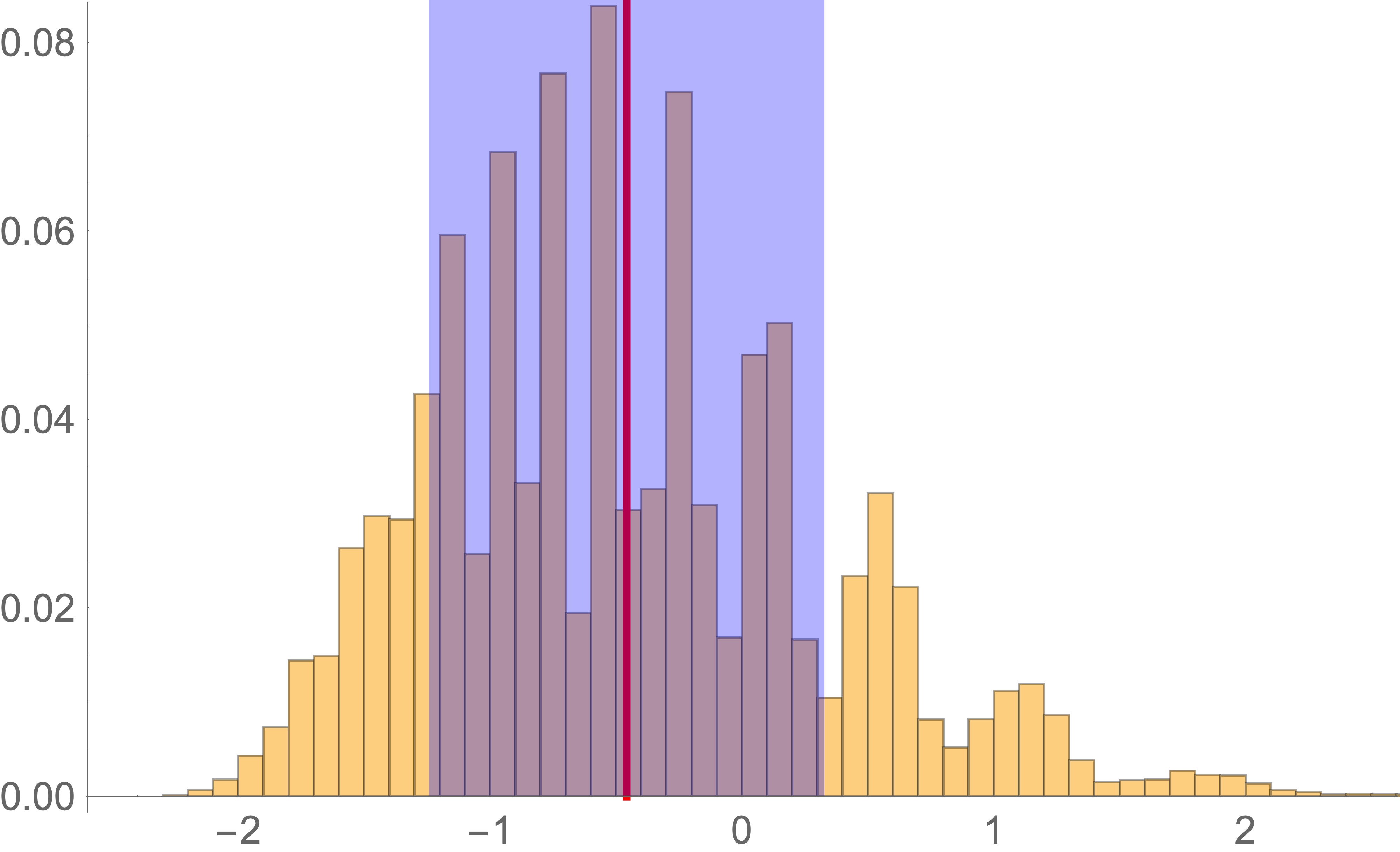
(a) $n=10^{2}$, $m=-0.4586$, $s=0.7844$

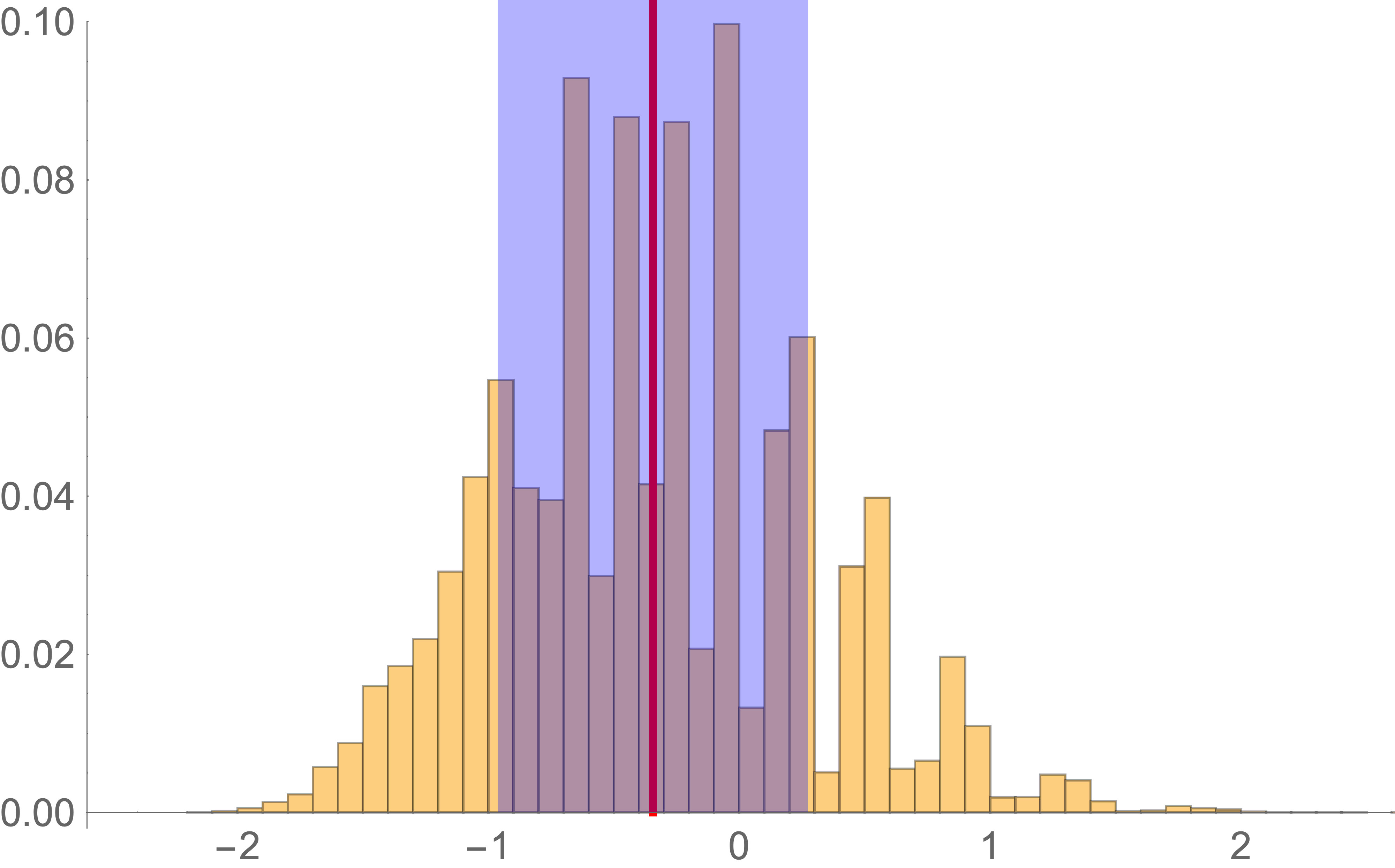
(b) $n=10^{3}$, $m=-0.3449$, $s=0.6175$

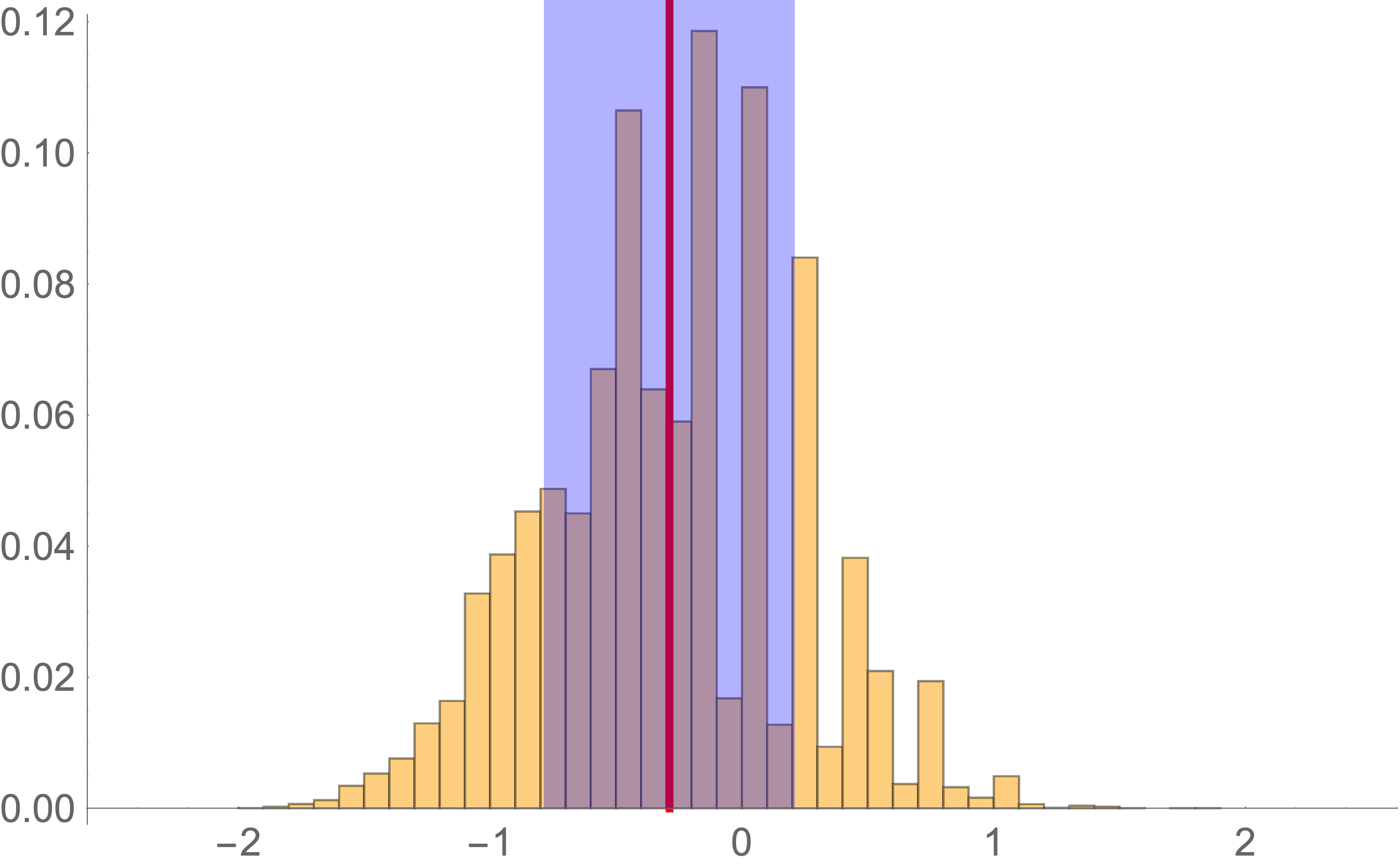
(c) $n=10^{4}$, $m=-0.2881$, $s=0.4976$

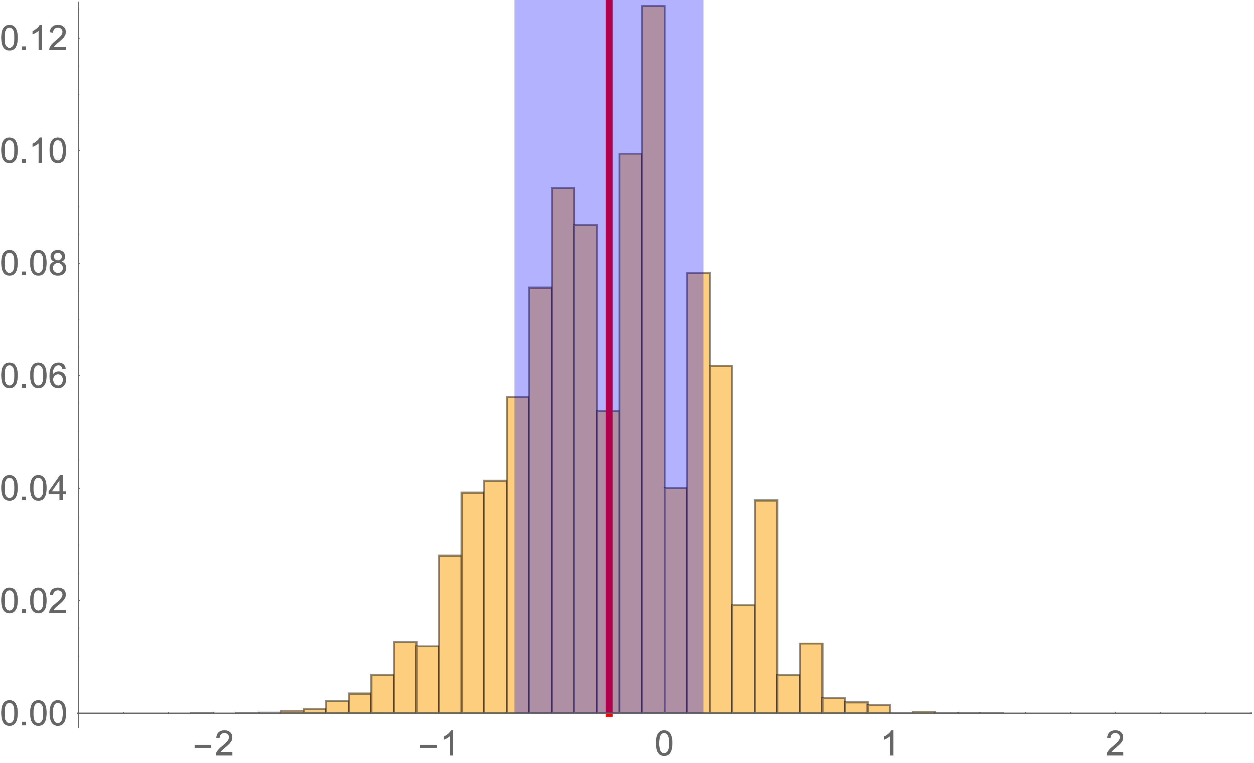
(d) $n=10^{5}$, $m=-0.2465$, $s=0.4186$

Figure 1: Empirical distribution of $\lambda_{n,V}\left(\frac{\omega_{1}\left|\ln F(0)\right|}{\ln n}\right)^{-2}-\mu_{1}$ for $d=1$ and $V(0)\overset{\text{d}}{=}$ Bernoulli$(0.3)$ computed form $10^{5}$ samples. The empirical mean ($m$) and empirical standard deviation ($s$) are shown in red and blue respectively.

Our second result is a partial proof of Conjecture ‣ 1, and a complete proof when $d=1$.

Theorem 2.

• $\displaystyle\varliminf_{n\to\infty}\lambda_{n,V}\left\|L_{n,V}\right\|_{\infty}\geq\frac{\mu_{d}}{2d}$ $\mathbb{P}$-a.s.

• If $d=1$ then $\displaystyle\lim_{n\to\infty}\lambda_{n,V}\left\|L_{n,V}\right\|_{\infty}=\frac{\mu_{1}}{2}$ $\mathbb{P}$-a.s.

Remark.

The preprint [CWZ21] has a proof of ii) in the continuous setting for the (C1) case. Both proofs follow the heuristic of the largest ball with zero or very low potential, but differ on how to obtain the lower bound of $\lambda_{n,V}$ and the upper bound of $L_{n,V}$.

We prove Theorem 2 in Section 3 after deriving some general properties of landscape functions. Most notable among these properties is Proposition 9, which states that $\lambda_{A,W}\left\|L_{A,W}\right\|_{\infty}$ is bounded form above and bellow by two dimensional constants uniformly on $A$ and $W$. This is a consequence of an upper bound of the $\ell^{\infty}\to\ell^{\infty}$ norm of the semigroup generated by the Schrödinger operator, which we adapted from the book [Szn98] to the discrete setting. The statement i) of Theorem 2 follows from domain monotonicity of the landscape function and the asymptotic of $\lambda_{n,V}$ given in Theorem 1, while ii) is based on the geometric resolvent identity and the restrictions of one dimensional geometry. In Figure 2 we illustrate ii) by showing the convergence of the empirical distribution of $\lambda_{n,V}\left\|L_{n,V}\right\|_{\infty}-\frac{\mu_{1}}{2}$ towards $0$.

In the proofs that follow, $C(d)$ is a finite positive constant that may only depend on the dimension and can change form line to line. By $a_{t}\sim_{t}b_{t}$ we mean $\lim_{t\to\infty}\frac{a_{t}}{b_{t}}=1$.

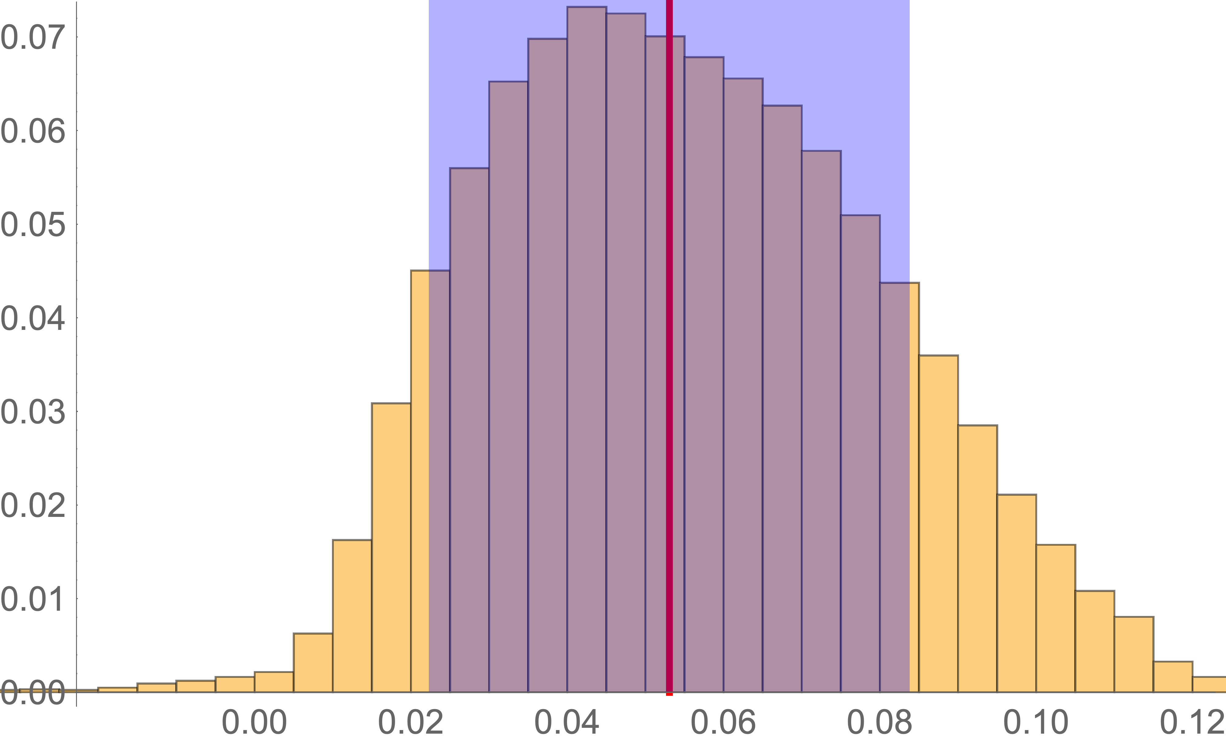
(a) $n=10^{2}$, $m=5.3\times 10^{-2}$, $s=3.0\times 10^{-2}$

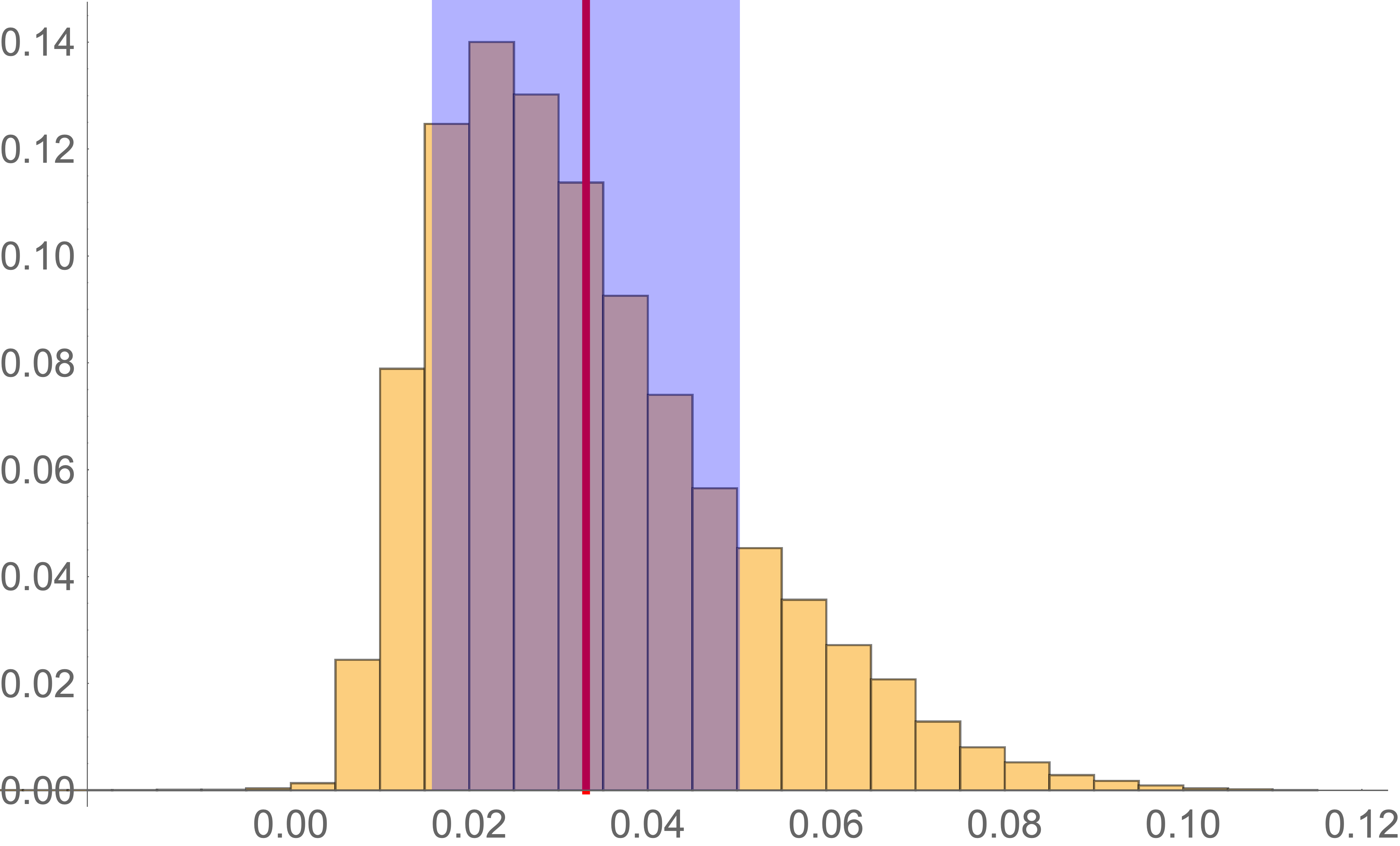
(b) $n=10^{3}$, $m=3.3\times 10^{-2}$, $s=1.7\times 10^{-2}$

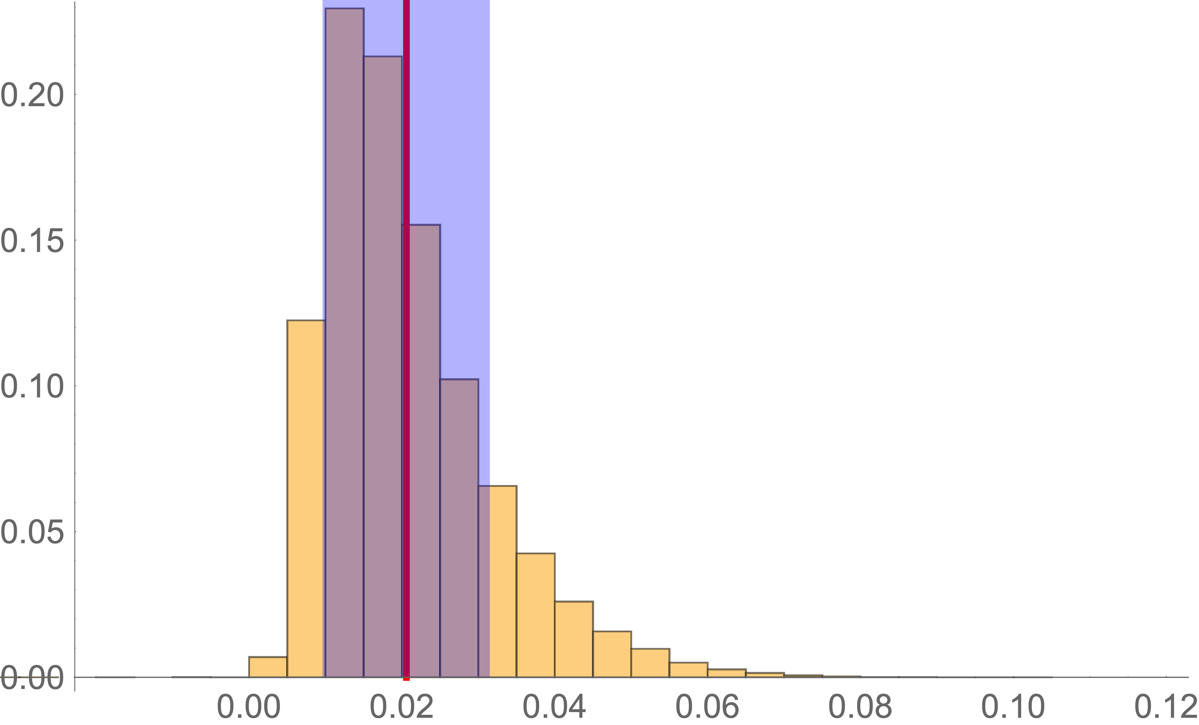
(c) $n=10^{4}$, $m=2.0\times 10^{-2}$, $s=1.0\times 10^{-2}$

(d) $n=10^{5}$, $m=1.3\times 10^{-2}$, $s=7.3\times 10^{-3}$

Figure 2: Empirical distribution of $\lambda_{n,V}\left\|L_{n,V}\right\|_{\infty}-\frac{\mu_{1}}{2}$ for $d=1$ and $V(0)\overset{\text{d}}{=}$ Bernoulli$(0.3)$ computed form $10^{5}$ samples. The empirical mean ($m$) and empirical standard deviation ($s$) are shown in red and blue respectively.

2 Principal Eigenvalue (Proof of Theorem 1)

2.1 Upper Bound of $\lambda_{n,V}$

We introduce the sequences

$$\varepsilon_{n}\coloneqq\begin{cases}0,&\textbf{(C1)},\\ (\ln n)^{-2/d},&\textbf{(C2)},\end{cases}\qquad y_{n}\coloneqq\left(\frac{d\ln n}{\omega_{d}\left|\ln F(\varepsilon_{n})\right|}\right)^{1/d},$$

so we can write the goal of this subsection as

$$\varlimsup_{n\to\infty}y_{n}^{2}\lambda_{n,V}\leq\mu_{d}\quad\mathbb{P}\text{-a.s.}$$ (1)

As usual, getting a sharp upper bound on $\lambda_{n,V}$ is much easier than a sharp lower bound. It just requires choosing a good test function and applying the Min-Max Principle.

Let $Y_{n}$ be the radius of the largest open euclidean ball contained in $\Lambda_{n}$ in which $V$ is uniformly bounded by $\varepsilon_{n}$, that is,

$$Y_{n}\coloneqq\max\left\{r\in\mathbb{N}\,\middle|\,\exists x\in\Lambda_{n}\,\text{ such that }\,B(x,r)\cap\mathbb{Z}^{d}\subseteq\Lambda_{n}\cap V^{-1}\big{(}[0,\varepsilon_{n}]\big{)}\right\},$$

where $B(x,r)=\{x^{\prime}\in\mathbb{R}^{d}\,|\,\left|x-x^{\prime}\right|<r\}\subseteq\mathbb{R}^{d}$. Also, let $x_{n}\in\Lambda_{n}$ be the center of a ball at which the maximum is attained (it may not be unique). The asymptotic growth of $Y_{n}$ is given in the next proposition, whose proof we delay a short moment.

Proposition 3.

$\displaystyle Y_{n}\sim_{n}y_{n}$ $\mathbb{P}$-a.s.

Let $\phi\in\ell^{2}(B(x_{n},Y_{n})\cap\mathbb{Z}^{d})$ be the normalized eigenvector of $-\Delta_{B(x_{n},Y_{n})}$ associated to $\lambda_{B(x_{n},Y_{n})\cap\mathbb{Z}^{d},0}$ and extend it by $0$ to $\Lambda_{n}$. Then, by the Min-Max Principle, we have

$$\lambda_{n,V} \leq\left\langle\phi,\left(-\Delta_{n}+V\right)\phi\right\rangle_{\ell^{2}(\Lambda_{n})}=\left\langle\phi,\left(-\Delta_{B(x_{n},Y_{n})\cap\mathbb{Z}^{d}}+V\right)\phi\right\rangle_{\ell^{2}(B(x_{n},Y_{n})\cap\mathbb{Z}^{d})}$$

$$\leq\lambda_{B(x_{n},Y_{n})\cap\mathbb{Z}^{d},0}+\varepsilon_{n}$$

and therefore

$$\varlimsup_{n\to\infty}y_{n}^{2}\lambda_{n,V}\leq\lim_{n\to\infty}y_{n}^{2}\left(\lambda_{B(x_{n},Y_{n})\cap\mathbb{Z}^{d},0}+\varepsilon_{n}\right)=\lim_{n\to\infty}\frac{y_{n}^{2}}{Y_{n}^{2}}Y_{n}^{2}\lambda_{B(x_{n},Y_{n})\cap\mathbb{Z}^{d},0}=\mu_{d}\quad\mathbb{P}\text{-a.s.},$$

where we have used Proposition 3, $\displaystyle\lim_{r\to\infty}r^{2}\lambda_{B(0,r)\cap\mathbb{Z}^{d},0}=\mu_{d}$ and translation invariance. This last limit is a consequence of the discrete Laplacian converging to the continuous one, or random walk converging to Brownian motion. A proof following the latter approach can be found in [LL10, Proposition 8.4.2], where an extra factor $d$ appears as a result of the probabilistic normalization of the Laplacian.

Proof of Proposition 3.

If $Y_{n}<y_{n}(1-\delta)^{1/d}$ for some $0<\delta<1$, then the inscribed ball of each of the $\left(\frac{2n}{2y_{n}(1-\delta)^{1/d}}\right)^{d}(1+o(1))$ disjoint cubes, of side length $\left\lceil 2y_{n}(1-\delta)^{1/d}\right\rceil$, that make up $\Lambda_{n}$ contains a point $x$ with $V(x)>\varepsilon_{n}$. Approximating the number of points in such balls by $\#(B(0,r)\cap\mathbb{Z}^{d})\sim_{r}\operatorname{Vol}(B(0,r))=\omega_{d}r^{d}$, we obtain for large $n$

$$\mathbb{P}\left[Y_{n}<y_{n}(1-\delta)^{1/d}\right] \leq\left(1-F(\varepsilon_{n})^{\omega_{d}y_{n}^{d}(1-\delta)(1+o(1))}\right)^{\frac{n^{d}}{y_{n}^{d}(1-\delta)}(1+o(1))}$$

$$=\left(1-\frac{1}{n^{d(1-\delta)(1+o(1))}}\right)^{\frac{n^{d}\omega_{d}\left|\ln F(\varepsilon_{n})\right|}{d(\ln n)(1-\delta)}(1+o(1))}$$

$$\leq\exp\left(-\frac{n^{\delta}\omega_{d}\left|\ln F(\varepsilon_{n})\right|}{2d(\ln n)(1-\delta)}\right),$$

which is summable. Therefore, the Borel–Cantelli Lemma and sending $\delta\to 0$ give

$$1\leq\varliminf_{n\to\infty}y_{n}^{-1}Y_{n}\quad\mathbb{P}\text{-a.s.}$$

We show the $\limsup$ bound first on an exponential sub-sequence and then we extend it to the whole sequence. The extending argument requires a monotone sequence of random variables, which $Y_{n}$ may fail to be if (C2) holds. For this reason we introduce

$$Y_{n,n^{\prime}}\coloneqq\max\left\{r\in\mathbb{N}\,\middle|\,\exists x\in\Lambda_{n}\,\text{ such that }\,B(x,r)\cap\mathbb{Z}^{d}\subseteq\Lambda_{n}\cap V^{-1}\big{(}[0,\varepsilon_{n^{\prime}}]\big{)}\right\},$$

which is increasing on $n$, decreasing on $n^{\prime}$ and satisfies $Y_{n,n}=Y_{n}$. Since for $\delta>0$ and large $m$ we have

$$\mathbb{P}\left[Y_{\left\lfloor e^{m+1}\right\rfloor,\left\lfloor e^{m}\right\rfloor}>y_{\left\lfloor e^{m}\right\rfloor}(1+\delta)^{1/d}\right] \leq\sum_{x\in\Lambda_{\left\lfloor e^{m+1}\right\rfloor}}\mathbb{P}\left[B(x,y_{\left\lfloor e^{m}\right\rfloor}(1+\delta)^{1/d})\cap\mathbb{Z}^{d}\subseteq V^{-1}[0,\varepsilon_{\left\lfloor e^{m}\right\rfloor}]\right]$$

$$=\#\Lambda_{\left\lfloor e^{m+1}\right\rfloor}F(\varepsilon_{\left\lfloor e^{m}\right\rfloor})^{\omega_{d}y_{\left\lfloor e^{m}\right\rfloor}^{d}(1+\delta)(1+o(1))}$$

$$=\frac{\#\Lambda_{\left\lfloor e^{m+1}\right\rfloor}}{\left\lfloor e^{m}\right\rfloor^{d(1+\delta)(1+o(1))}}$$

$$\leq C(d)e^{-md\delta/2},$$

the Borel–Cantelli Lemma and the limit $\delta\to 0$ give

$$\varlimsup_{m\to\infty}y_{\left\lfloor e^{m}\right\rfloor}^{-1}Y_{\left\lfloor e^{m+1}\right\rfloor,\left\lfloor e^{m}\right\rfloor}\leq 1\quad\mathbb{P}\text{-a.s.}$$

For $n\in\mathbb{N}$ define $m(n)\in\mathbb{N}$ by $\left\lfloor e^{m(n)}\right\rfloor\leq n<\left\lfloor e^{m(n)+1}\right\rfloor$. Since $y_{n}\sim_{n}y_{\left\lfloor e^{m(n)}\right\rfloor}$ and $Y_{n}\leq Y_{\left\lfloor e^{m(n)+1}\right\rfloor,\left\lfloor e^{m(n)}\right\rfloor}$ we conclude

$$\varlimsup_{n\to\infty}y_{n}^{-1}Y_{n}\leq\varlimsup_{n\to\infty}y_{n}^{-1}Y_{\left\lfloor e^{m(n)+1}\right\rfloor,\left\lfloor e^{m(n)}\right\rfloor}=\varlimsup_{n\to\infty}y_{\left\lfloor e^{m(n)}\right\rfloor}^{-1}Y_{\left\lfloor e^{m(n)+1}\right\rfloor,\left\lfloor e^{m(n)}\right\rfloor}\leq 1\quad\mathbb{P}\text{-a.s.}\qed$$

2.2 Lower Bound of $\lambda_{n,V}$

In this subsection we show that $\mathbb{P}$-a.s. we have

$$1\leq\varliminf_{n\to\infty}\frac{\lambda_{n,V}}{\mu_{d}\left(\frac{\omega_{d}\left|\ln F(0)\right|}{d\ln n}\right)^{2/d}}\qquad\text{and}\qquad 1\leq\varliminf_{n\to\infty}\frac{\lambda_{n,V}}{\mu_{d}\left(\frac{2\eta\omega_{d}\ln\ln n}{d^{2}\ln n}\right)^{2/d}}$$ (2)

for (C1) and (C2) respectively. The main input for this is a Lifshitz tail result on the integrated density of states from [BK01]. We recall the integrated density of states of the Anderson model is a deterministic distribution function given by the $\mathbb{P}$-a.s. limit

$$I(t)\coloneqq\lim_{n\to\infty}\frac{1}{\#\Lambda_{n}}\#\{\lambda\in\sigma(-\Delta_{n}+V)\,|\,\lambda\leq t\},\qquad t\in\mathbb{R},$$

where the eigenvalues are counted with multiplicities. The central hypothesis of [BK01] is a scaling assumption of the cumulant-generating function $H(t)\coloneqq\ln\mathbb{E}\left[e^{-tV(0)}\right]$ of $V(0)$, which we prove in the following proposition. To state it, we first need to define

$$(1,\infty)\ni t\longmapsto\alpha(t)\coloneqq\begin{cases}t^{1/(d+2)},&\textbf{(C1)},\\ \left(\frac{t}{\ln t}\right)^{1/(d+2)},&\textbf{(C2)},\end{cases}\qquad\widetilde{H}\coloneqq\begin{cases}\left|\ln F(0)\right|,&\textbf{(C1)},\\ \frac{2\eta}{d+2},&\textbf{(C2)}.\end{cases}$$

Proposition 4.

For any compact $K\subseteq(0,\infty)$ we have

$$\lim_{t\to\infty}\frac{\alpha^{d+2}(t)}{t}H\left(\frac{t}{\alpha^{d}(t)}y\right)=-\widetilde{H}$$

uniformly on $y\in K$.

Proof.

First assume (C1). In this case $\frac{\alpha^{d+2}(t)}{t}=1$ and $\frac{t}{\alpha^{d}(t)}=t^{2/(d+2)}$. Since for $t>0$ we have

$$\ln F(0)\leq H(t) =\ln\left(\mathbb{E}\left[e^{-tV(0)}\mathds{1}_{V(0)\leq\frac{1}{\sqrt{t}}}\right]+\mathbb{E}\left[e^{-tV(0)}\mathds{1}_{V(0)>\frac{1}{\sqrt{t}}}\right]\right)$$

$$\leq\ln\left(F\left(1/\sqrt{t}\right)+e^{-\sqrt{t}}\right),$$

we conclude that

$$\sup_{y\in K}\left|\frac{\alpha^{d+2}(t)}{t}H\left(\frac{t}{\alpha^{d}(t)}y\right)-\ln F(0)\right| \leq\sup_{y\in K}\ln\left(F\left(\frac{1}{t^{1/d+2}\sqrt{y}}\right)+e^{-t^{1/d+2}\sqrt{y}}\right)-\ln F(0)$$

$$=\ln\left(F\left(\frac{1}{t^{1/d+2}\sqrt{\min K}}\right)+e^{-t^{1/d+2}\sqrt{\min K}}\right)-\ln F(0)$$

$$\quad\xrightarrow[t\to\infty]{}0.$$

Now assume (C2). In this case $\frac{\alpha^{d+2}(t)}{t}=\frac{1}{\ln t}$ and $\frac{t}{\alpha^{d}(t)}=t^{2/(d+2)}(\ln t)^{d/(d+2)}$. We introduce a parameter $0<\delta<1$ and observe

$$H(t)=\ln\left(\mathbb{E}\left[e^{-tV(0)}\mathds{1}_{V(0)\leq t^{-\delta}}\right]+\mathbb{E}\left[e^{-tV(0)}\mathds{1}_{V(0)>t^{-\delta}}\right]\right)\leq\ln\left(F\left(t^{-\delta}\right)+e^{-t^{1-\delta}}\right),\qquad t>0,$$

which implies

$$\varlimsup_{t\to\infty}\sup_{y\in K}\frac{\alpha^{d+2}(t)}{t}H\left(\frac{t}{\alpha^{d}(t)}y\right)$$

$$\qquad\leq\varlimsup_{t\to\infty}\sup_{y\in K}\frac{1}{\ln t}\ln\left(F\left(\left[\frac{t}{\alpha^{d}(t)}y\right]^{-\delta}\right)+\exp\left(-\left[\frac{t}{\alpha^{d}(t)}y\right]^{1-\delta}\right)\right)$$

$$\qquad=\varlimsup_{t\to\infty}\frac{1}{\ln t}\ln\left(F\left(\left[\frac{t}{\alpha^{d}(t)}\min K\right]^{-\delta}\right)+\exp\left(-\left[\frac{t}{\alpha^{d}(t)}\min K\right]^{1-\delta}\right)\right)$$

$$\qquad=-\frac{2\delta\eta}{d+2}\xrightarrow[\delta\to 1]{}-\frac{2\eta}{d+2}.$$

For the $\displaystyle\varliminf_{t\to\infty}\inf_{y\in K}$ we use

$$H(t)=\ln\left(\mathbb{E}\left[e^{-tV(0)}\mathds{1}_{V(0)\leq t^{-1}}\right]+\mathbb{E}\left[e^{-tV(0)}\mathds{1}_{V(0)>t^{-1}}\right]\right)\geq\ln\left(e^{-1}F(t^{-1})\right),\qquad t>0$$

to obtain

$$\varliminf_{t\to\infty}\inf_{y\in K}\frac{\alpha^{d+2}(t)}{t}H\left(\frac{t}{\alpha^{d}(t)}y\right) \geq\varliminf_{t\to\infty}\inf_{y\in K}\frac{1}{\ln t}\ln\left(e^{-1}F\left(\left[\frac{t}{\alpha^{d}(t)}y\right]^{-1}\right)\right)$$

$$\geq\varliminf_{t\to\infty}\frac{1}{\ln t}\ln\left(e^{-1}F\left(\left[\frac{t}{\alpha^{d}(t)}\max K\right]^{-1}\right)\right)=-\frac{2\eta}{d+2}.\qed$$

Having checked the scaling assumption on $H$, we now have the Lifshitz tail result:

Theorem 5 (Theorem 1.3 of [BK01]).

Define $\displaystyle\chi\coloneqq\inf_{g\in H^{1}(\mathbb{R}^{d}),\,\left\|g\right\|_{2}=1}\left(\left\|\nabla g\right\|_{2}^{2}+\widetilde{H}\operatorname{Vol}(\operatorname{supp}g)\right)$, then

$$\lim_{t\downarrow 0}\frac{\ln I(t)}{t\alpha^{-1}\left(t^{-1/2}\right)}=-2\,d^{d/2}\left(\frac{\chi}{d+2}\right)^{(d+2)/2}.$$

Remark.

The function $t\mapsto\alpha(t)$ is eventually increasing so $\alpha^{-1}(t)$ is well defined for large $t$. The original statement from [BK01] is far more general; our conditions on $V$ make $H$ fall into, what is there called, the $(\gamma=0)$-class.

The constant $\chi$ can be explicitly computed by means of the Faber-Krahn inequality:

Proposition 6.

$\displaystyle\chi=(d+2)\left(\frac{\widetilde{H}\omega_{d}}{2}\right)^{2/(d+2)}\left(\frac{\mu_{d}}{d}\right)^{d/(d+2)}$.

Proof.

Starting from $\chi=\inf_{g\in H^{1}(\mathbb{R}^{d}),\,\left\|g\right\|_{2}=1}\left(\left\|\nabla g\right\|_{2}^{2}+D\operatorname{Vol}(\operatorname{supp}g)\right)$ we see that we only need to consider the finite volume case. Hence

$$\chi=\inf_{\begin{subarray}{c}A\subseteq\mathbb{R}^{d},\\ \operatorname{Vol}(A)<\infty\end{subarray}}\inf_{\begin{subarray}{c}g\in H^{1}(\mathbb{R}^{d}),\,\left\|g\right\|_{2}=1,\\ \operatorname{supp}g=A\end{subarray}}\left(\left\|\nabla g\right\|_{2}^{2}+\widetilde{H}\operatorname{Vol}(A)\right)=\inf_{\begin{subarray}{c}A\subseteq\mathbb{R}^{d},\\ \operatorname{Vol}(A)<\infty\end{subarray}}\left(\mu(A)+\widetilde{H}\operatorname{Vol}(A)\right),$$

where $\mu(A)$ is the principal eigenvalue of the continuous Laplacian ($-\sum_{i=1}^{d}\partial^{2}/\partial x_{i}^{2}$) defined on $A$ with Dirichlet boundary conditions. The Faber-Krahn inequality states that over all domains of a given volume the one with the lowest principal eigenvalue is the ball, therefore, using $\mu(B(0,r))=\mu_{d}/r^{2}$ and $\operatorname{Vol}(B(0,r))=\omega_{d}r^{d}$ we obtain

$$\chi=\inf_{0<r<\infty}\left(\frac{\mu_{d}}{r^{2}}+\widetilde{H}\omega_{d}r^{d}\right).$$

Evaluating at the only critical point $\displaystyle r=\left(\frac{2\mu_{d}}{\widetilde{H}\omega_{d}d}\right)^{1/(d+2)}$ finishes the proof. ∎

We now exploit the connection between $I$ and the distribution of $\lambda_{n,V}$. This is a classic argument that can be found, for instance, in [AW15, Equation 4.46]. We present here a slightly modified version. Let $n\in\mathbb{N}$ and define a new potential

$$V^{\prime}(x)\coloneqq\begin{cases}\infty,&x\in(2n+2)\mathbb{Z}^{d},\\ V(x),&\text{else}.\end{cases}$$

Clearly $V\leq V^{\prime}$ so for any $k\in\mathbb{N}$ and $t\in\mathbb{R}$ we have

$$\frac{\#\{\lambda\in\sigma(-\Delta_{(2n+2)k}+V)\,|\,\lambda\leq t\}}{\#\Lambda_{(2n+2)k}}\geq\frac{\#\{\lambda\in\sigma(-\Delta_{(2n+2)k}+V^{\prime})\,|\,\lambda\leq t\}}{\#\Lambda_{(2n+2)k}}$$

where we use implicitly the convention of Dirichlet boundary conditions wherever $V^{\prime}$ is infinite. Taking $k\to\infty$ and noting that the infinities of $V^{\prime}$ decompose $-\Delta_{(2n+2)k}+V^{\prime}$ in to a direct sum of $(2k)^{d}$ independent terms equal in distribution to $-\Delta_{n}+V$ we obtain

$$I(t) \geq\left(\lim_{k\to\infty}\frac{(2k)^{d}}{\#\Lambda_{(2n+2)k}}\right)\mathbb{E}\left[\#\{\lambda\in\sigma(-\Delta_{n}+V)\,|\,\lambda\leq t\}\right]$$

$$\geq\left(\frac{1}{2n+2}\right)^{d}\mathbb{P}\left[\lambda_{n,V}\leq t\right].$$

From the previous inequality, Theorem 5 and Proposition 6 we have

$$\mathbb{P}\left[\lambda_{n,V}\leq t\right]\leq C(d)n^{d}I(t)\leq C(d)\,n^{d}\exp\left[-f(1/t)(1+o(1))\right]\quad\text{as }t\downarrow 0,$$ (3)

where we have introduced $\displaystyle f(t)\coloneqq\frac{\widetilde{H}\omega_{d}\mu_{d}^{d/2}\alpha^{-1}(t^{1/2})}{t}$. To finish the proof we need the asymptotic of $f^{-1}(t)$ as $t\to\infty$:

Proposition 7.

• For (C1), $\displaystyle f^{-1}(t)=\frac{1}{\mu_{d}}\left(\frac{t}{\omega_{d}\left|\ln F(0)\right|}\right)^{2/d}$.

• For (C2), $\displaystyle f^{-1}(t)\sim_{t}\frac{1}{\mu_{d}}\left(\frac{d\,t}{2\eta\omega_{d}\ln t}\right)^{2/d}$.

Proof.

For (C1) there is nothing to prove since $f(t)=\omega_{d}\left|\ln F(0)\right|\mu_{d}^{d/2}t^{d/2}$. For (C2) we have

$$f(t)=\frac{k\alpha^{-1}(t^{1/2})}{t}=kt^{d/2}\ln\alpha^{-1}(t^{1/2}),$$

with all the constants collected in $k=\frac{2\eta\omega_{d}\mu_{d}^{d/2}}{d+2}$. Since $\alpha$ is eventually increasing and has infinite limit, the same is true for $f$, in particular $f^{-1}(t)$ exists for large $t$. By solving for the $\alpha^{-1}$ term in the first equality above, applying $\alpha$ and simplifying some exponents we arrive at $t=\left(\frac{f(t)}{k\ln\left[tf(t)/k\right]}\right)^{2/d}$. Replacing $t$ by $f^{-1}(t)$ we obtain

$$f^{-1}(t)=\left(\frac{t}{k\ln\left[tf^{-1}(t)/k\right]}\right)^{2/d},$$

and then multiplying by $t$ and taking the logarithm leads to

$$\ln[tf^{-1}(t)]=\frac{d+2}{d}\ln t-\frac{2}{d}\ln\left[k\ln\left[tf^{-1}(t)/k\right]\right],$$

which implies

$$f^{-1}(t)\sim_{t}\left(\frac{d\,t}{(d+2)k\ln t}\right)^{2/d}=\frac{1}{\mu_{d}}\left(\frac{d\,t}{2\eta\omega_{d}\ln t}\right)^{2/d}.\qed$$

Going back to (3) with $n=\left\lfloor e^{m}\right\rfloor$ and $t=1/f^{-1}((1+\delta)dm)$ for some $m\in\mathbb{N}$ and $\delta>0$, we see that

$$\mathbb{P}\left[\lambda_{\left\lfloor e^{m}\right\rfloor,V}f^{-1}((1+\delta)dm)\leq 1\right] \leq C(d)\left(\left\lfloor e^{m}\right\rfloor\right)^{d}\exp\left[-(1+\delta)dm(1+o(1))\right]$$

$$\leq C(d)\,e^{-md\delta/2},$$

which is summable over $m\in\mathbb{N}$. Therefore, by the Borel–Cantelli Lemma we have

$$1\leq\varliminf_{m\to\infty}\lambda_{\left\lfloor e^{m}\right\rfloor,V}f^{-1}((1+\delta)dm)=(1+\delta)^{2/d}\varliminf_{m\to\infty}\lambda_{\left\lfloor e^{m}\right\rfloor,V}f^{-1}(dm)\quad\mathbb{P}\text{-a.s.}$$

As in the proof of Proposition 3, we define $m(n)\in\mathbb{N}$ by $\left\lfloor e^{m(n)}\right\rfloor\leq n<\left\lfloor e^{m(n)+1}\right\rfloor$, so that $\ln n\sim_{n}(m(n)+1)$. Since $n\mapsto\lambda_{n,V}$ is monotone decreasing we have

$$\varliminf_{n\to\infty}\lambda_{n,V}f^{-1}(d\ln n) \geq\varliminf_{n\to\infty}\lambda_{\left\lfloor e^{m(n)+1}\right\rfloor,V}f^{-1}(d\ln n)$$

$$=\varliminf_{n\to\infty}\lambda_{\left\lfloor e^{m(n)+1}\right\rfloor,V}f^{-1}(d(m(n)+1))\geq(1+\delta)^{-2/d}\quad\mathbb{P}\text{-a.s.}$$

By sending $\delta\to 0$ and replacing the $f^{-1}$ term by its asymptotic given in Proposition 7 we obtain the desired result of this subsection.

3 Landscape Function

We start this section by deriving some general properties of landscape functions.

For a finite $A\subseteq\mathbb{Z}^{d}$ and $W:A\rightarrow[0,\infty)$ we introduce the Green function (with $0$ as spectral parameter)

$$G_{A,W}(x,y)\coloneqq\begin{cases}\left\langle\delta_{x},(-\Delta_{A}+W)^{-1}\delta_{y}\right\rangle_{\ell^{2}(A)},&(x,y)\in A\times A,\\ 0,&(x,y)\in(\mathbb{Z}^{d}\times\mathbb{Z}^{d})\setminus(A\times A).\end{cases}$$

This function is known to be symmetric, non-negative, decreasing on the potential $W$; and to satisfy the geometric resolvent identity (see [Kir08, Section 5.3]): if $A^{\prime}\subseteq A$ then

$$G_{A,W}(x,y)=G_{A^{\prime},W}(x,y)+\sum_{(i,j)\in\partial A^{\prime}}G_{A^{\prime},W}(x,i)G_{A,W}(j,y),$$

where $\partial A^{\prime}\coloneqq\{(i,j)\in\mathbb{Z}^{d}\times\mathbb{Z}^{d}\,|\,i\in A^{\prime},\,j\notin A^{\prime},\,\left|i-j\right|=1\}$ is the boundary of $A^{\prime}$. By extending the definition of $L_{A,W}$ to $L_{A,W}(x)\coloneqq\sum_{y\in\mathbb{Z}^{d}}G_{A,W}(x,y)$ for all $x\in\mathbb{Z}^{d}$, the previously stated properties of $G_{A,W}$ translate into non-negativity, potential monotonicity and domain monotonicity of landscape functions:

• $L_{A,W}\geq 0$ and $L_{A,W}(x)=0$ if $x\in\mathbb{Z}^{d}\setminus A$.

• If $0\leq W^{\prime}\leq W$ then $L_{A,W}\leq L_{A,W^{\prime}}$.

• If $A^{\prime}\subseteq A$ then

  $$L_{A,W}(x)=L_{A^{\prime},W}(x)+\sum_{(i,j)\in\partial A^{\prime}}G_{A^{\prime},W}(x,i)L_{A,W}(j)\geq L_{A^{\prime},W}(x).$$ (4)

Our last general property is that $\lambda_{A,W}\left\|L_{A,W}\right\|_{\infty}$ is bounded from above and bellow by two positive constants uniformly on $A$ and $W$. This is based on the following upper bound of the $\ell^{\infty}\to\ell^{\infty}$ norm of the semigroup, which can be found, for the continuous setting, in [Szn98, Chapter 3, Theorem 1.2]. We could not find a proof in the literature for the discrete case, so we provide one in Appendix A.

Theorem 8.

For any finite $A\subseteq\mathbb{Z}^{d}$ and $W:A\rightarrow[0,\infty)$ we have

$$\left\|\exp\left(-t[-\Delta_{A}+W]\right)\mathds{1}_{A}\right\|_{\infty}\leq C(d)\left(1+\left[\lambda_{A,W}t\right]^{d/2}\right)\exp\left(-\lambda_{A,W}t\right),\qquad t\geq 0.$$

As an an immediate consequence we obtain:

Proposition 9.

For any finite $A\subseteq\mathbb{Z}^{d}$ and $W:A\rightarrow[0,\infty)$ we have

$$1\leq\lambda_{A,W}\left\|L_{A,W}\right\|_{\infty}\leq C(d).$$

Remark.

The lower bound is sharp. It is attained when $A$ is a single point of $\mathbb{Z}^{d}$.

Proof.

For the upper bound we use Theorem 8 and the substitution $u=\lambda_{A,W}t$:

$$\left\|L_{A,W}\right\|_{\infty} =\left\|\int_{0}^{\infty}\exp\left(-t[-\Delta_{A}+W]\right)\mathds{1}_{A}\,\mathrm{d}t\right\|_{\infty}$$

$$\leq C(d)\int_{0}^{\infty}\left(1+\left[\lambda_{A,W}t\right]^{d/2}\right)\exp\left(-\lambda_{A,W}t\right)\,\mathrm{d}t$$

$$=\frac{C(d)}{\lambda_{A,W}}\int_{0}^{\infty}\left(1+u^{d/2}\right)e^{-u}\,\mathrm{d}u=\frac{C(d)}{\lambda_{A,W}}.$$

For the lower bound we just need to notice that the positivity of $G_{A,W}$ implies

$$\sup_{\phi\in\ell^{2}(A)\setminus\{0\}}\frac{\left\|(-\Delta_{A}+W)^{-1}\phi\right\|_{\infty}}{\left\|\phi\right\|_{\infty}}=\sup_{\phi\in\ell^{2}(A)\setminus\{0\}}\frac{\left\|\sum_{y\in A}G_{A,W}(\cdot,y)\phi(y)\right\|_{\infty}}{\left\|\phi\right\|_{\infty}}=\left\|L_{A,W}\right\|_{\infty}.$$

By plugging in the eigenvector associated to $\lambda_{A,W}$ we obtain $\left\|L_{A,W}\right\|_{\infty}\geq\frac{1}{\lambda_{A,W}}$. ∎

3.1 Proof of Theorem 2 i)

We start with the asymptotic of the sup-norm of the landscape function on balls with $0$ potential.

Proposition 10.

$\displaystyle\left\|L_{B(0,r)\cap\mathbb{Z}^{d},0}\right\|_{\infty}\sim_{r}\frac{r^{2}}{2d}$.

Proof.

Let $r>0$ and consider the function $\phi_{r}(x)\coloneqq\frac{r^{2}-\left|x\right|^{2}}{2d}$ defined on $\mathbb{Z}^{d}$. Clearly $-\Delta\phi_{r}(x)=1$ for all $x\in\mathbb{Z}^{d}$ and therefore $L_{B(0,r)\cap\mathbb{Z}^{d},0}-\phi_{r}$ is harmonic in $B(0,r)\cap\mathbb{Z}^{d}$. By the Maximum Principle we have

$$\left|\left\|L_{B(0,r)\cap\mathbb{Z}^{d},0}\right\|_{\infty}-\frac{r^{2}}{2d}\right| =\left|\sup_{x\in B(0,r)\cap\mathbb{Z}^{d}}L_{B(0,r)\cap\mathbb{Z}^{d},0}(x)-\sup_{x\in B(0,r)\cap\mathbb{Z}^{d}}\phi_{r}(x)\right|$$

$$\leq\sup_{x\in B(0,r)\cap\mathbb{Z}^{d}}\left|L_{B(0,r)\cap\mathbb{Z}^{d},0}(x)-\phi_{r}(x)\right|$$

$$=\sup_{x\in\partial^{+}\left[B(0,r)\cap\mathbb{Z}^{d}\right]}\left|L_{B(0,r)\cap\mathbb{Z}^{d},0}(x)-\phi_{r}(x)\right|$$

$$=\sup_{x\in\partial^{+}\left[B(0,r)\cap\mathbb{Z}^{d}\right]}\left|\phi_{r}(x)\right|\leq C(d)\,r(1+o(1))$$

where $\partial^{+}A\coloneqq\left\{x\in\mathbb{Z}^{d}\setminus A\,\middle|\,\exists\,y\in A\text{ such that }\left|x-y\right|=1\right\}$ is the outer boundary of $A\subseteq\mathbb{Z}^{d}$. Dividing by $\frac{r^{2}}{2d}$ and taking the limit $r\to\infty$ give the proposition. ∎

Recall the definitions of $\varepsilon_{n}$, $Y_{n}$, $x_{n}$ and $y_{n}$ from Subsection 2.1 and notice that Theorem 1 can be restated as $\lambda_{n,V}\sim_{n}\frac{\mu_{d}}{y_{n}^{2}}$ $\mathbb{P}$-a.s. From domain monotonicity of landscape functions we have

$$L_{n,V}\geq L_{B(x_{n},Y_{n})\cap\mathbb{Z}^{d},V}.$$

For (C1), $V$ is identically $0$ in $B(x_{n},Y_{n})\cap\mathbb{Z}^{d}$ so Theorem 1, Proposition 10 and translation invariance give

$$\varliminf_{n\to\infty}\lambda_{n,V}\left\|L_{n,V}\right\|_{\infty}\geq\lim_{n\to\infty}\lambda_{n,V}\left\|L_{B(x_{n},Y_{n})\cap\mathbb{Z}^{d},0}\right\|_{\infty}=\lim_{n\to\infty}\frac{\mu_{d}}{y_{n}^{2}}\frac{Y_{n}^{2}}{2d}=\frac{\mu_{d}}{2d}\quad\mathbb{P}\text{-a.s.}$$

For (C2), we use the second resolvent identity, domain monotonicity of the eigenvalue, and Propositions 9, 10, 3 to obtain

$$\lambda_{n,V}\left\|L_{B(x_{n},Y_{n})\cap\mathbb{Z}^{d},0}-L_{B(x_{n},Y_{n})\cap\mathbb{Z}^{d},V}\right\|_{\infty} =\lambda_{n,V}\left\|(-\Delta_{B(x_{n},Y_{n})\cap\mathbb{Z}^{d},0})^{-1}VL_{B(x_{n},Y_{n})\cap\mathbb{Z}^{d},V}\right\|_{\infty}$$

$$\leq C(d)\varepsilon_{n}\left\|L_{B(x_{n},Y_{n})\cap\mathbb{Z}^{d},0}\right\|_{\infty}$$

$$\leq C(d)\varepsilon_{n}Y_{n}^{2}\xrightarrow[n\to\infty]{\mathbb{P}\text{-a.s.}}0,$$

which implies

$$\varliminf_{n\to\infty}\lambda_{n,V}\left\|L_{n,V}\right\|_{\infty} \geq\lim_{n\to\infty}\lambda_{n,V}\left\|L_{B(x_{n},Y_{n})\cap\mathbb{Z}^{d},V}\right\|_{\infty}$$

$$=\lim_{n\to\infty}\lambda_{n,V}\left\|L_{B(x_{n},Y_{n})\cap\mathbb{Z}^{d},0}\right\|_{\infty}=\frac{\mu_{d}}{2d}\quad\mathbb{P}\text{-a.s.}$$

This concludes the proof of Theorem 2 i).

3.2 Proof of Theorem 2 ii)

We assume from this point on that $d=1$. We set $\llbracket a,b\rrbracket\coloneqq[a,b]\cap\mathbb{Z}$ for any two $a,b\in\mathbb{Z}$. This proof is based on the following deterministic bound of the Green function in terms of the values of the potential.

Proposition 11.

Let $n\in\mathbb{N}$ and $W:\llbracket 1,n\rrbracket\rightarrow[0,\infty)$. For any $y\in\llbracket 1,n\rrbracket$ we have

$$G_{\llbracket 1,n\rrbracket,W}(1,y) \leq\left(\sum_{j=0}^{y-1}(y-j)W(y-j)\right)^{-1},$$

$$G_{\llbracket 1,n\rrbracket,W}(y,n) \leq\left(\sum_{j=0}^{n-y}(n-y+1-j)W(y+j)\right)^{-1}.$$

Proof.

We only prove the first inequality; the second one follows from reflecting $W$ across the midpoint of $\llbracket 1,n\rrbracket$ and the symmetry of the Green function.

Fix some $y\in\llbracket 1,n\rrbracket$. By potential monotonicity we have $G_{\llbracket 1,n\rrbracket,W}\leq G_{\llbracket 1,n\rrbracket,W\mathds{1}_{\llbracket 1,y\rrbracket}}$. The Cramer’s rule lets us write

$$G_{\llbracket 1,n\rrbracket,W\mathds{1}_{\llbracket 1,y\rrbracket}}(1,y)=\frac{\det\left([-\Delta_{\llbracket 1,n\rrbracket}+W\mathds{1}_{\llbracket 1,y\rrbracket}]_{1\to\delta_{y}}\right)}{\det(-\Delta_{\llbracket 1,n\rrbracket}+W\mathds{1}_{\llbracket 1,y\rrbracket})},$$

where $[-\Delta_{\llbracket 1,n\rrbracket}+W\mathds{1}_{\llbracket 1,y\rrbracket}]_{1\to\delta_{y}}$ is the matrix obtained by replacing the first column (in the canonical $\delta_{j}$ basis) of $-\Delta_{\llbracket 1,n\rrbracket}+W\mathds{1}_{\llbracket 1,y\rrbracket}$ by $\delta_{y}$. By computing the determinant from such first column we see that

$$\det\left([-\Delta_{\llbracket 1,n\rrbracket}+W\mathds{1}_{\llbracket 1,y\rrbracket}]_{1\to\delta_{y}}\right) =(-1)^{y+1}\det\left(\begin{array}[]{c|c}T&0\\ \hline\cr M&-\Delta_{\llbracket 1,n-y\rrbracket}\end{array}\right)$$

$$=(-1)^{y+1}\det(T)\det(-\Delta_{\llbracket 1,n-y\rrbracket})=n-y+1,$$

since $T$ is a lower triangular square matrix of size $y-1$ with $(-1)$ on all the diagonal, and $\det(-\Delta_{\llbracket 1,k\rrbracket})=k+1$ for all $k\in\mathbb{N}$ (we use the convention $\det(-\Delta_{\varnothing})=1$).

Consider $\det(-\Delta_{\llbracket 1,n\rrbracket}+W\mathds{1}_{\llbracket 1,y\rrbracket})$ as a polynomial in $(W(j))_{j=1}^{y}$. It is clear that it does not contain squares, or grater powers, of any $W(j)$. Moreover, the coefficient of the monomial $W(j_{1})W(j_{2})\cdots W(j_{k-1})W(j_{k})$ with $1\leq j_{1}<j_{2}<\ldots j_{k-1}<j_{k}\leq y$ and $k\geq 1$ can easily be computed as

$$\det(-\Delta_{\llbracket 1,j_{1}-1\rrbracket}) \det(-\Delta_{\llbracket j_{1}+1,j_{2}-1\rrbracket})\cdots\det(-\Delta_{\llbracket j_{k-1}+1,j_{k}-1\rrbracket})\det(-\Delta_{\llbracket j_{k}+1,n\rrbracket})$$

$$=j_{1}(j_{2}-j_{1})\cdots(j_{k}-j_{k-1})(n+1-j_{k}).$$

The remaining constant coefficient is $\det(-\Delta_{\llbracket 1,n\rrbracket})=n+1$, which means all coefficients of $\det(-\Delta_{\llbracket 1,n\rrbracket}+W\mathds{1}_{\llbracket 1,y\rrbracket})$ are positive and therefore

$$G_{\llbracket 1,n\rrbracket,W}(1,y) \leq\frac{n+1-y}{\det(-\Delta_{\llbracket 1,n\rrbracket}+W\mathds{1}_{\llbracket 1,y\rrbracket})}\leq\frac{n+1-y}{\sum_{j=1}^{y}j(n+1-j)W(x)}$$

$$\leq\left(\sum_{j=1}^{y}jW(j)\right)^{-1}=\left(\sum_{j=0}^{y-1}(y-j)W(y-j)\right)^{-1}.\qed$$

With the previous proposition in mind we define for $\delta>0$ and $x\in\mathbb{Z}^{d}$

$$Z^{+}_{\delta}(x) \coloneqq\min\left\{n\in\mathbb{N}\,\middle|\,\sum_{j=1}^{n}(n+1-j)V(x+j)>\delta^{-1}\right\},$$

$$Z^{-}_{\delta}(x) \coloneqq\min\left\{n\in\mathbb{N}\,\middle|\,\sum_{j=1}^{n}(n+1-j)V(x-j)>\delta^{-1}\right\},$$

$$A_{\delta}(x) \coloneqq\llbracket x-Z^{-}_{\delta}(x),x+Z^{+}_{\delta}(x)\rrbracket.$$

Notice that $V(x)$ is not included in the definition of $Z^{\pm}_{\delta}(x)$ and therefore $Z^{+}_{\delta}(x)$ and $Z^{-}_{\delta}(x)$ are independent for all $x\in\mathbb{Z}$.

It follows from (4), the definitions above, potential monotonicity, and Propositions 9, 11 that

$$\lambda_{n,V}\left\|L_{n,V}\right\|_{\infty} \leq\lambda_{n,V}\max_{x\in\Lambda_{n}}\left[L_{A_{\delta}(x),0}(x)+2\delta\left\|L_{n,V}\right\|_{\infty}\right]$$

$$\leq\lambda_{n,V}\max_{x\in\Lambda_{n}}\left\|L_{A_{\delta}(x),0}\right\|_{\infty}+2\delta C(1).$$

By domain monotonicity and translation invariance, the last maximum above is attained at the $x\in\Lambda_{n}$ that also maximises $\#A_{\delta}(x)=Z^{+}_{\delta}(x)+Z^{-}_{\delta}(x)+1$. Moreover, $V$ being i.i.d. implies $\lim_{n\to\infty}\max_{x\in\Lambda_{n}}Z^{+}_{\delta}(x)+Z^{-}_{\delta}(x)=\infty\quad\mathbb{P}$-a.s. and therefore Proposition 10 and Theorem 1 give

$$\varlimsup_{n\to\infty}\lambda_{n,V}\left\|L_{n,V}\right\|_{\infty}\leq\frac{\mu_{1}}{2}\varlimsup_{n\to\infty}\left(\frac{\max_{x\in\Lambda_{n}}Z^{+}_{\delta}(x)+Z^{-}_{\delta}(x)}{2y_{n}}\right)^{2}+2\delta C(1)\quad\mathbb{P}\text{-a.s.}$$

The proof of Theorem 2 ii) is finished with the next proposition followed by the limit $\delta\to 0$.

Proposition 12.

For all $\delta>0$, $\displaystyle\varlimsup_{n\to\infty}\frac{1}{2y_{n}}\max_{x\in\Lambda_{n}}[Z^{+}_{\delta}(x)+Z^{-}_{\delta}(x)]\leq 1\quad\mathbb{P}$-a.s.

Proof.

We will prove this over an exponential subsequence; the extension is done as in the proof of Proposition 3 using the monotonicity of $n\mapsto\max_{x\in\Lambda_{n}}[Z^{+}_{\delta}(x)+Z^{-}_{\delta}(x)]$. In addition to $Z^{+}_{\delta}(x)$ being independent of $Z^{-}_{\delta}(x)$ for all $x\in\mathbb{Z}^{d}$, we also have that all $Z^{\pm}_{\delta}(x)$ are equal in distribution to $Z^{+}_{\delta}(0)$.

Assume (C1). For all $t>0$ we have

$$\mathbb{E}\left[e^{-tV(0)}\right]=\mathbb{E}\left[e^{-tV(0)}\mathds{1}_{V(0)\leq\frac{1}{\sqrt{t}}}\right]+\mathbb{E}\left[e^{-tV(0)}\mathds{1}_{V(0)>\frac{1}{\sqrt{t}}}\right]\leq F\left(1/\sqrt{t}\right)+e^{-\sqrt{t}}.$$

With this, we use the exponential Markov inequality and independence to obtain

$$\mathbb{P}\left[Z_{\delta}^{+}(0)>n\right] =\mathbb{P}\left[\sum_{j=1}^{n}(n+1-j)V(x+j)^{-1}\leq\delta^{-1}\right]$$

$$\leq e^{t/\delta}\prod_{j=1}^{n}\mathbb{E}\left[\exp(-tjV(0))\right]\leq e^{t/\delta}\left(F\left(1/\sqrt{t}\right)+e^{-\sqrt{t}}\right)^{n},\qquad n\in\mathbb{N}.$$

Now we proceed with the distribution of $Z^{+}_{\delta}(0)+Z^{-}_{\delta}(0)$ as

$$\mathbb{P}\left[Z^{+}_{\delta}(0)+Z^{-}_{\delta}(0)>n\right] =\mathbb{P}\left[Z^{+}_{\delta}(0)>n-1\right]+\sum_{j=1}^{n-1}\mathbb{P}\left[Z^{+}_{\delta}(0)=j\right]\mathbb{P}\left[Z^{-}_{\delta}(0)>n-j\right]$$

$$\leq 2\mathbb{P}\left[Z^{+}_{\delta}(0)>n-1\right]+\sum_{j=2}^{n-1}\mathbb{P}\left[Z^{+}_{\delta}(0)>j-1\right]\mathbb{P}\left[Z^{+}_{\delta}(0)>n-j\right]$$

$$\leq 2e^{t/\delta}\left(F\left(1/\sqrt{t}\right)+e^{-\sqrt{t}}\right)^{n-1}+(n-2)e^{2t/\delta}\left(F\left(1/\sqrt{t}\right)+e^{-\sqrt{t}}\right)^{n-1}$$

$$\leq ne^{2t/\delta}\left(F\left(1/\sqrt{t}\right)+e^{-\sqrt{t}}\right)^{n-1}.$$

For any $\varepsilon>0$ define $t(\varepsilon)$ by $\ln\left(F\left(1/\sqrt{t(\varepsilon)}\right)+e^{-\sqrt{t(\varepsilon)}}\right)\leq\frac{\ln F(0)}{1+\varepsilon}$ so that

$$\mathbb{P}\left[\max_{x\in\Lambda_{n}}[Z^{+}_{\delta}(x)+Z^{-}_{\delta}(x)]>\left\lfloor(1+\varepsilon)^{2}2y_{n}\right\rfloor\right] \leq C(1)n\,\mathbb{P}\left[Z^{+}_{\delta}(0)+Z^{-}_{\delta}(0)>\left\lfloor(1+\varepsilon)^{2}2y_{n}\right\rfloor\right]$$

$$\leq C(1)e^{2t(\varepsilon)/\delta}n\exp\left[(1+\varepsilon)^{2}2y_{n}\frac{\ln F(0)}{1+\varepsilon}(1+o(1))\right]$$

$$=C(1)e^{2t(\varepsilon)/\delta}n^{-\varepsilon(1+o(1))},$$

which is summable over the exponential subsequence $n=\left\lfloor e^{m}\right\rfloor$, $m\in\mathbb{N}$.

Assume (C2). We follow the same steps as for (C1) above. To bound the Laplace transform of $V(0)$ we consider the function $f(t)\coloneqq a[F(t)]^{1/\eta}$ for some $a>0$. From (C2) follows that there exists $t_{0}\in(0,\infty)$ such that $F(t)\leq 2\,c\,t^{\eta}$ for all $t\in[0,t_{0}]$. Therefore, by choosing $a\coloneqq(t_{0}^{-1}+(2c)^{1/\eta})^{-1}$ we obtain

$$0\leq f(t)\leq\begin{cases}a(2c)^{1/\eta}t\leq t,&t\in[0,t_{0}],\\ a\leq t_{0}\leq t,&t\in(t_{0},\infty).\end{cases}$$

Moreover, since $\mathbb{P}\left[f(V(0))\leq t\right]=\left(\frac{t}{a}\right)^{\eta}$ for $t\in[0,a]$, we have

$$\mathbb{E}\left[\exp(-tV(0))\right] \leq\mathbb{E}\left[\exp(-tf(V(0)))\right]=\frac{\eta}{(a)^{\eta}}\int_{0}^{a}e^{-ty}y^{\eta-1}\,\mathrm{d}y$$

$$\leq\frac{\eta}{(a)^{\eta}}\int_{0}^{\infty}e^{-ty}y^{\eta-1}\,\mathrm{d}y=\frac{\eta\Gamma(\eta)}{(at)^{\eta}},\qquad t>0.$$

The exponential Markov inequality at $t=n\eta\delta$, independence, and the Stirling bound $(n/e)^{n}\leq n!$ lead us to

$$\mathbb{P}\left[Z_{\delta}^{+}(0)>n\right] \leq e^{t/\delta}\prod_{j=1}^{n}\mathbb{E}\left[\exp(-tjV(0))\right]\leq\left(\frac{\eta\Gamma(\eta)}{(at)^{\eta}}\right)^{n}\frac{e^{t/\delta}}{(n!)^{\eta}}$$

$$\leq\left(\frac{\eta^{1-\eta}\Gamma(\eta)e^{2\eta}}{a^{\eta}\delta}\right)^{n}n^{-2\eta n}\eqqcolon K_{\delta}^{n}\,n^{-2\eta n},\qquad n\in\mathbb{N},$$

from which follows

$$\mathbb{P}\left[Z^{+}_{\delta}(0)+Z^{-}_{\delta}(0)>n\right]\leq 2K_{\delta}^{n-1}(n-1)^{-2\eta(n-1)}+K_{\delta}^{n-1}\sum_{j=2}^{n-1}\left(j-1\right)^{-2\eta(j-1)}(n-j)^{-2\eta(n-j)}.$$

The function $[2,n-1]\ni j\mapsto\left(j-1\right)^{-(j-1)}(n-j)^{-(n-j)}$ attains its unique maximum at $j=(n+1)/2$, therefore

$$\mathbb{P}\left[Z^{+}_{\delta}(0)+Z^{-}_{\delta}(0)>n\right] \leq 2K_{\delta}^{n-1}(n-1)^{-2\eta(n-1)}+(4^{\eta}K_{\delta})^{n-1}(n-2)(n-1)^{-2\eta(n-1)}$$

$$\leq(4^{\eta}K_{\delta})^{n-1}n(n-1)^{-2\eta(n-1)}.$$

Finally, for $\varepsilon>0$ we have

$$\mathbb{P}\left[\max_{x\in\Lambda_{n}}[Z^{+}_{\delta}(x)+Z^{-}_{\delta}(x)]>\left\lfloor(1+\varepsilon)2y_{n}\right\rfloor\right] \leq C(1)n\,\mathbb{P}\left[Z^{+}_{\delta}(0)+Z^{-}_{\delta}(0)>\left\lfloor(1+\varepsilon)2y_{n}\right\rfloor\right]$$

$$=C(1)n\exp\left[-(1+\varepsilon)4\eta y_{n}(\ln y_{n})(1+o(1))\right]$$

$$=C(1)n\exp\left[-(1+\varepsilon)4\eta y_{n}(\ln\ln n)(1+o(1))\right]$$

$$=C(1)n^{-\varepsilon(1+o(1))},$$

which is summable over the exponential subsequence $n=\left\lfloor e^{m}\right\rfloor$, $m\in\mathbb{N}$. ∎

Appendix A Proof of Theorem 8

Let $(X_{t})_{t\geq 0}$ be a continuous time simple symmetric random walk on $\mathbb{Z}^{d}$ with jump intensity $1$, and let $\mathrm{P}_{x}$, $\mathrm{E}_{x}$ be the associated probability measure and expectation conditioned on $X_{0}=x$. We remark that $(X_{t})_{t\geq 0}$ is the Markov process that generates $-\Delta/(2d)$ on $\ell^{2}(\mathbb{Z}^{d})$.

For a finite $A\subseteq\mathbb{Z}^{d}$ and $W:A\rightarrow[0,\infty)$, the Feynman–Kac formula lets us write the semigroup generated by $-\Delta_{A}+W$ as

$$\exp\left(-\frac{t}{2d}[-\Delta_{A}+W]\right)\phi(x)=\mathrm{E}_{x}\left[\phi(X_{t})\exp\left(-\int_{0}^{t}\frac{W(X_{s})}{2d}\,\mathrm{d}s\right)\mathds{1}_{t<\tau_{A}}\right],\quad\phi\in\ell^{2}(A),\,x\in A,$$

where $\tau_{A}\coloneqq\inf\{t\geq 0\,|\,X_{t}\notin A\}$ is the exit time of $A$. To simplify notation we set $\lambda=\frac{\lambda_{A,W}}{2d}$, $K_{t}=\exp\left(-\frac{t}{2d}[-\Delta_{A}+W]\right)$ and $k_{t}(x,y)=\left\langle\delta_{x},K_{t}\delta_{y}\right\rangle_{\ell^{2}(A)}$ (the kernel of the semigroup). Depending on $\lambda$ we distinguish two cases.

• Case $\lambda\leq\frac{1}{d}$.

Let $\overline{B_{\infty}}(x,r)\coloneqq\{y\in\mathbb{R}^{d}\,|\,\left\|x-y\right\|_{\infty}\leq r\}$. For $t\geq 1$ and $x\in A$ we have

$$K_{t/\lambda}\mathds{1}_{A}(x) =K_{t/\lambda}\mathds{1}_{A\cap\overline{B_{\infty}}(x,r)}(x)+K_{t/\lambda}\mathds{1}_{A\setminus\overline{B_{\infty}}(x,r)}(x)$$

$$\leq\left\langle k_{1/\lambda}(x,\cdot),K_{(t-1)/\lambda}\mathds{1}_{A\cap\overline{B_{\infty}}(x,r)}\right\rangle_{\ell^{2}(A)}+\mathrm{P}_{0}\left[X_{t/\lambda}\notin\overline{B_{\infty}}(0,r)\right]$$

$$\leq C(d)\sqrt{\mathrm{P}_{0}\left[X_{2/\lambda}=0\right]}r^{d/2}e^{-(t-1)}+\mathrm{P}_{0}\left[X_{t/\lambda}\notin\overline{B_{\infty}}(0,r)\right],$$

where we chose $r=2t\sqrt{\frac{e}{\lambda d}}$.

The term $\mathrm{P}_{0}\left[X_{2/\lambda}=0\right]$ can be estimated using the characteristic function of $X_{s}$, which is $\phi_{s}(\theta)=\exp\left(-s+\frac{s}{d}\sum_{i=1}^{d}\cos(\theta_{i})\right)$, by means of

$$\mathrm{P}_{0}\left[X_{s}=0\right]=\frac{1}{(2\pi)^{d}}\int_{[-\pi,\pi]^{d}}\phi_{s}(\theta)\,\mathrm{d}\theta=\frac{e^{-s}}{(2\pi)^{d}}\left[\int_{[-\pi,\pi]}\exp\left(\frac{s}{d}\cos\theta_{1}\right)\,\mathrm{d}\theta_{1}\right]^{d}.$$

Laplace’s method applied to the right-most integral yields $\mathrm{P}_{0}\left[X_{s}=0\right]s^{d/2}\xrightarrow[s\to\infty]{}\left(\frac{d}{2\pi}\right)^{d/2}$ and therefore $\mathrm{P}_{0}\left[X_{2/\lambda}=0\right]\leq C(d)\lambda^{d/2}$.

For the other probability we use the bound (see [Bar17, Lemma 4.6])

$$P[S_{n}>y]\leq e^{-y^{2}/(2n)},\qquad y>0,$$

where $S_{n}$ is a discrete time simple symmetric random walk on $\mathbb{Z}$ starting at $0$, and $P$ is its probability measure. Recalling that the first component of $X_{t}$, which we denote $X_{t}^{1}$, is a continuous time simple symmetric random walk on $\mathbb{Z}$ with jump intensity $1/d$ we have

$$\mathrm{P}_{0}\left[X_{t/\lambda}\notin\overline{B_{\infty}}(0,r)\right]\leq 2d\mathrm{P}_{0}\left[X_{t/\lambda}^{1}>r\right]\leq 2d\sum_{n\geq 0}\frac{e^{-t/(\lambda d)}}{n!}\left(\frac{t}{\lambda d}\right)^{n}P[S_{n}>r].$$

We split the series at $n=\frac{2et}{\lambda d}$ and bound the two terms separately:

$$\sum_{n\leq\frac{2et}{\lambda d}}\frac{e^{-t/(\lambda d)}}{n!}\left(\frac{t}{\lambda d}\right)^{n}P[S_{n}>r] \leq\sum_{n\leq\frac{2et}{\lambda d}}\frac{e^{-t/(\lambda d)}}{n!}\left(\frac{t}{\lambda d}\right)^{n}e^{-r^{2}/(2n)}$$

$$\leq\exp\left(-\frac{r^{2}\lambda d}{4et}\right)\sum_{n\leq\frac{2et}{\lambda d}}\frac{e^{-t/(\lambda d)}}{n!}\left(\frac{t}{\lambda d}\right)^{n}\leq\exp\left(-\frac{r^{2}\lambda d}{4et}\right)=e^{t},$$

$$\sum_{n\geq\frac{2et}{\lambda d}}\frac{e^{-t/(\lambda d)}}{n!}\left(\frac{t}{\lambda d}\right)^{n}P[S_{n}>r] \leq e^{-t/(\lambda d)}\sum_{n\geq\frac{2et}{\lambda d}}\frac{1}{n!}\left(\frac{t}{\lambda d}\right)^{n}$$

$$\leq e^{-t/(\lambda d)}\sum_{n\geq 0}\frac{1}{n!}\left(\frac{n}{2e}\right)^{n}\leq C(1)e^{-t}.$$

With this we have shown $\left\|K_{t/\lambda}\mathds{1}_{A}\right\|_{\infty}\leq C(d)\left(1+t^{d/2}\right)e^{-t}$ for $t\geq 1$. Since $K_{t/\lambda}\mathds{1}(x)$ is always bounded by $1$ we can add $\left(\inf_{0\leq t\leq 1}\left(1+t^{d/2}\right)e^{-t}\right)^{-1}$ to $C(d)$, if necessary, to have

$$\left\|K_{t/\lambda}\mathds{1}_{A}\right\|_{\infty}\leq C(d)\left(1+t^{d/2}\right)e^{-t},\qquad t\geq 0.$$

Replacing $t$ by $2d\lambda t$ and gives the desired bound.

• Case $\lambda\geq\frac{1}{d}$.

This case follows form the heat kernel bound (see [Bar17, Theorem 5.17])

$$\mathrm{P}_{0}\left[X_{t}=y\right]\leq C(d)\exp\left[-t-\left\|y\right\|_{1}\ln\left(\frac{\left\|y\right\|_{1}}{et}\right)\right],\qquad\left\|y\right\|_{1}\geq et.$$

We proceed as before but now we use $\overline{B_{1}}(x,r)\coloneqq\{y\in\mathbb{R}^{d}\,|\,\left\|x-y\right\|_{1}\leq r\}$. For $t\geq 0$ we have

$$K_{t}\mathds{1}_{A}(x) =K_{t}\mathds{1}_{A\cap\overline{B_{1}}(x,r)}(x)+K_{t}\mathds{1}_{A\setminus\overline{B_{1}}(x,r)}(x)$$

$$\leq\left\langle\delta_{x},K_{t}\mathds{1}_{A\cap\overline{B_{1}}(x,r)}\right\rangle_{\ell^{2}(A)}+\mathrm{P}_{0}\left[X_{t}\notin\overline{B_{1}}(0,r)\right]$$

$$\leq C(d)r^{d/2}e^{-\lambda t}+\mathrm{P}_{0}\left[X_{t}\notin\overline{B_{1}}(0,r)\right],$$

with $r=\lambda tde^{2}$. Clearly $r\geq et$, so we can apply the heat kernel bound to obtain

$$\mathrm{P}_{0}\left[X_{t}^{1}\notin\overline{B_{1}}(0,r)\right] \leq C(d)\sum_{\begin{subarray}{c}y\in\mathbb{Z}^{d}\\ \left\|y\right\|_{1}>r\end{subarray}}\exp\left[-t-\left\|y\right\|_{1}\ln\left(\frac{\left\|y\right\|_{1}}{et}\right)\right]$$

$$\leq C(d)\sum_{\begin{subarray}{c}y\in\mathbb{Z}^{d}\\ \left\|y\right\|_{1}>r\end{subarray}}\exp\left[-\left\|y\right\|_{1}\ln(ed)\right]$$

$$\leq C(d)e^{-r}\sum_{y\in\mathbb{Z}^{d}}\exp\left[-\left\|y\right\|_{1}\right]$$

$$=C(d)e^{-r}\leq C(d)e^{-\lambda t},$$

and therefore $\left\|K_{t}\mathds{1}_{A}\right\|_{\infty}\leq C(d)\left(1+[\lambda t]^{d/2}\right)e^{-\lambda t}$. Replacing $t$ by $2dt$ and gives the desired bound.

References

[ADF+19]
Douglas N. Arnold, Guy David, Marcel Filoche, David Jerison, and Svitlana
Mayboroda.
Computing spectra without solving eigenvalue problems.
SIAM Journal on Scientific Computing, 41(1):B69–B92, 2019.
[ADJ+16]
Douglas N. Arnold, Guy David, David Jerison, Svitlana Mayboroda, and Marcel
Filoche.
Effective confining potential of quantum states in disordered media.
Phys. Rev. Lett., 116:056602, 2016.
[AW15]
Michael Aizenman and Simone Warzel.
Random operators: disorder effects on quantum spectra and
dynamics, volume 168 of Graduate Studies in Mathematics.
American Mathematical Society, Providence, RI, 2015.
[Bar17]
Martin T. Barlow.
Random walks and heat kernels on graphs, volume 438 of London Mathematical Society Lecture Note Series.
Cambridge University Press, Cambridge, 2017.
[BK01]
Marek Biskup and Wolfgang König.
Long-time tails in the parabolic Anderson model with bounded
potential.
The Annals of Probability, 29(2):636 – 682, 2001.
[CWZ21]
Ilias Chenn, Wei Wang, and Shiwen Zhang.
Approximating the ground state eigenvalue via the effective
potential.
arXiv preprint arXiv:2107.04969, 2021.
[DFM21]
G. David, M. Filoche, and S. Mayboroda.
The landscape law for the integrated density of states.
Advances in Mathematics, 390:107946, 2021.
[FM12]
Marcel Filoche and Svitlana Mayboroda.
Universal mechanism for anderson and weak localization.
Proceedings of the National Academy of Sciences,
109(37):14761–14766, 2012.
[Kir08]
Werner Kirsch.
An invitation to random Schrödinger operators.
In Random Schrödinger operators, volume 25 of Panoramas
et Synthèses. Société Mathématique de France, Paris, 2008.
[LL10]
Gregory F. Lawler and Vlada Limic.
Random walk: a modern introduction, volume 123 of Cambridge Studies in Advanced Mathematics.
Cambridge University Press, Cambridge, 2010.
[Szn98]
Alain-Sol Sznitman.
Brownian motion, obstacles and random media.
Springer Monographs in Mathematics. Springer-Verlag, Berlin, 1998.