Discriminating Against Unrealistic Interpolations
in Generative Adversarial Networks

Abstract

Interpolations in the latent space of deep generative models is one of the standard tools to synthesize semantically meaningful mixtures of generated samples. As the generator function is non-linear, commonly used linear interpolations in the latent space do not yield the shortest paths in the sample space, resulting in non-smooth interpolations. Recent work has therefore equipped the latent space with a suitable metric to enforce shortest paths on the manifold of generated samples. These are often, however, susceptible of veering away from the manifold of real samples, resulting in smooth but unrealistic generation that requires an additional method to assess the sample quality along paths. Generative Adversarial Networks (GANs), by construction, measure the sample quality using its discriminator network. In this paper, we establish that the discriminator can be used effectively to avoid regions of low sample quality along shortest paths. By reusing the discriminator network to modify the metric on the latent space, we propose a lightweight solution for improved interpolations in pre-trained GANs.

1 Introduction

Deep generative models, a class of deep learning methods used to synthesize data representative of some observed but typically unknown data distribution, have in recent years seen a terrific increase in active research. As a consequence, some of these methods can now achieve truly stunning results, e.g., very realistic images depicting people or objects which don’t exist in real life. At the forefront among these are generative adversarial networks (GANs), a quickly expanding subclass of deep generative models following the seminal work by Goodfellow et al. [11], which are distinguished by their ability to not only learn to synthesize data, but also learn to assess how representative of the dataset the synthetic data is. These two learning processes are pitched against each other in an adversarial game, with the goal of the former being able to synthesize data so well that the latter can’t tell it apart from real data.

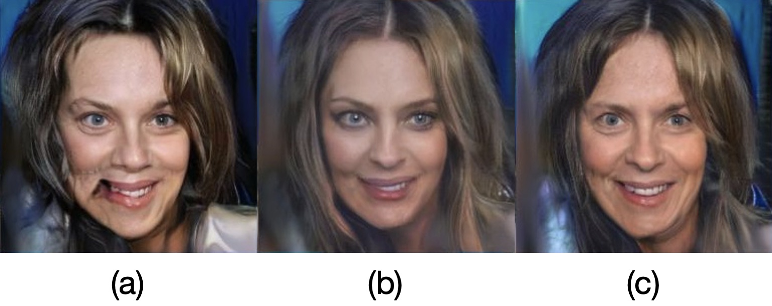
Figure 1: Single points on interpolated paths for ProGAN by Karras et al. [14] on CelebA-HQ using (a) Linear, (b) shortest path and (c) our approach. Full paths in Figure 9.

For many generative models, including GANs, the (so called) generator can be seen as producing samples on a lower dimensional manifold immersed in the high dimensional sample space. Similarly, we herein assume that the set of real data points, of which the dataset is a representative example, form a lower dimensional manifold immersed in sample space, however unknown. The goal of the generator is thereby not only to produce samples coinciding with the observed dataset, but to achieve perfect alignment between the generator and real data manifold.

Due to factors such as finite-size datasets, suboptimal training, choice of network architecture and its capacity, there will in general exist some degree of mismatch between these manifolds. One type of mismatch is commonly called mode collapse; when all points in latent space map to either a single, or too few, points in sample space, such that the generator’s output is apparently less rich than the real data manifold. In this work, we focus on another type of mismatch; when (the well-trained) generator occasionally produces unrealistic outputs, i.e., samples from outside of the real data manifold, as exemplified in Figure 1(a). This mismatch may be less obvious during training, but can be detrimental for interpolations in the latent space; a common post-processing tool for generating semantically meaningful data. E.g., using two latent points known to produce data with certain semantic features, one may use convex combinations (linear interpolations) of these to synthesize data where these features are mixed, see, e.g., Karras et al. [14] and Chen et al. [9]. Similarly, Bengio et al. [4] and Radford et al. [25], interpolate linearly between points and feature-dependent clusters identified post training.

If the latent space is equipped with a Euclidean metric, a linear interpolation defines a shortest path, i.e., a geodesic. The image of this path under the generator will however not, in general, be a shortest path on its manifold in sample space. One may instead equip the generator’s output space with a sensible and interpretable metric and pull this back to the latent space, thereby defining a Riemannian metric (see Arvanitidis [2] and Chen [8]). Searching for shortest paths in the latent space with respect to this newly defined metric will then lead to shortest paths on the manifold of the generator, but not necessarily on the true data manifold; causing the synthesis of unrealistic data, as illustrated in Figure 1(b), where the shortest path becomes blurry. To that end, this paper investigates a general yet simple approach to modify the Riemannian metric so that the mismatch between the generator and the true data manifold is taken into account, and a shortest path will only traverse regions of high data fidelity. For GANs, we show that a well-trained discriminator has the ability to provide gradient information between real and generated samples, and may thus be used as the modifier of the metric. Formulated as a machine learning method, the proposed method creates short and realistic interpolations between points in the latent space, see Figure 1(c).

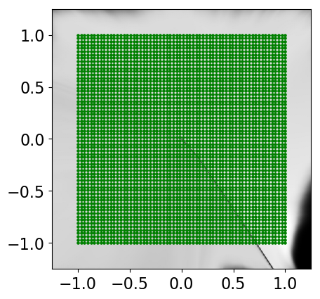
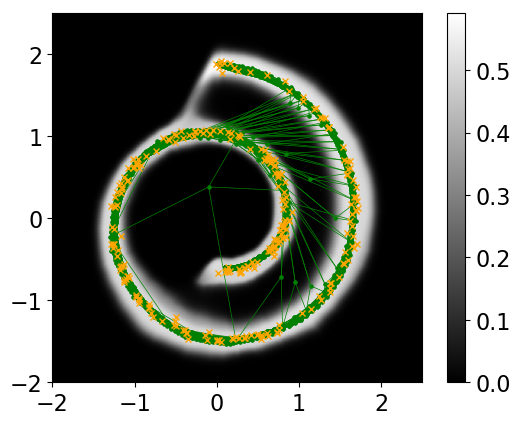
Figure 2: Latent space $Z$ (left) and the generator manifold $G(Z)$ (right) for the Swiss roll using a discrete grid of $64^{2}$ points. Orange $X$s and grayscale background denote real data points and discriminator values, respectively.

As a proof of concept, a toy example shows that mismatch of image and true data manifold already appears for simple problems; a GAN trained on the two-dimensional Swiss roll illustrates how the generator might learn a manifold larger than the data manifold (see Figure 2). Shortest paths on the image manifold thus fall off the Swiss roll, while the geodesics from our modified metric don’t. The proposed method is also implemented for ProGAN (by Karras et al. [14]) trained on the CelebA dataset (Liu et al. [21]), illustrating its ability to outperform both linear interpolations and shortest paths by producing realistic interpolations on the generator manifold.

2 Related work

It has been shown in a number of recent works that the proper way to measure distances in the latent space is to endow it with a Riemannian metric. Arvanitidis et al. [2] calculate shortest paths by solving an ordinary differential equation (ODE), applied to a variational autoencoder (or VAE, see [17]) to account for the curvature of the latent space. Subsequently, Yang et al. [32] show that a shortest path may also be found using a discrete analogue of the ODE in finite many sample points along the path. Both Shao et al. [27] and Chen et al. et al. [8] show similar results using discrete sample points. The latter work shows that linear interpolations are still serviceable, and hypothesises that the reason is that the curvature of the Riemannian metric is typically quite flat already, i.e., close to Euclidean. In subsequent work, Kühnel et al. [18] develop a framework for performing statistics (such as calculating the mean value) in a non-Euclidean latent space.

A number of works attempt to flatten or address the curvature of the latent space during training of the generator, thus improving linear interpolations. In the work by Berthelot et al. [5], the performance issues of autoencoders (see [26]) are improved by an additional network measuring image quality that is used to regularize the training of the autoencoder. Similarly, for VAEs, Chen et al. [7] proposed to flatten the generator manifold by replacing the VAEs standard Gaussian prior with a customized type of hierarchical prior. Using a different approach from the same authors, Chen et al. [6], approximate the generator manifold using a finite graph of generated samples and then use classical search algorithms to find the shortest paths. In a recent work, Stolberg-Larsen et al. [29] consider interpolations over partially disjoint generator manifolds, which could be used for datasets containing (partially disjoint) subclasses of data, for which Euclidean distances are ill-defined. Using a novel architecture of multiple generators, interpolations are done by matching the generator output using finite sample graphs. In two recent papers by Karras et al. [15, 16], the authors train a GAN using a generator architecture similar to networks performing style transfer to smoothly mix features between the images of faces or other objects using an intermediate latent space instead of the conventional latent space. To enforce smooth and realistic interpolations, the curvature of the intermediate latent space is regularized during training, thereby encouraging linear interpolations to be shortest paths. In this work, we will only consider traditional GAN architectures.

Two issues with the approaches above arise: Firstly, constraining the curvature might impede the quality of image generation, and secondly, it would be desirable to separate path finding from network training, as one may then reuse pre-trained networks. In a paper by Laine [19], shortest paths are found by pulling back the Euclidean metric on intermediary feature spaces in the VGG19 classification network [28], whose representations have been shown to correlate well with human perception [33]. Similarly, a recent work by Arvanitidis [3] studies suitable metrics on the sample space for defining the Riemannian pull-back metric. While their method is targeted toward probabilistic generators, they also consider how certain regions (in their example, blond people) can be effectively avoided in interpolating curves by assigning high cost to those regions. While our work was derived independently from their results, it may be considered as a continuation of their work, showing that the existing discriminator of a GAN is a suitable, yet simple ingredient to avoiding regions of unrealistic samples in interpolations.

3 Background

The mathematical convention around which deep generative modeling is built stems from statistical inference; the dataset serving as inspiration for the data synthesis is assumed to be a set of samples from some data distribution, i.e., ${\bf x}_{i}\sim p_{X},i=1,\dots,N,$ and the generative process attempts to draw new samples ${\bf x}$ from this distribution. Since the data distribution is generally intractable to model directly, the approach used in deep generative modeling is to construct a method for drawing samples from a conditional probability $p_{X|Z}({\bf x}|{\bf z})$, where a latent space $Z$ is equipped with a probability distribution $p_{Z}({\bf z})$ that is simple to sample from. The method for sampling from $p_{X|Z}$ exploits the immense capabilities of deep neural networks to approximate $p_{X|Z}$ with help of a generator function $G:Z\rightarrow X$. While the generator $G$ may be probabilistic for some generative models, for GANs, among others, the generator is constructed using a deterministic feed-forward network resulting in a degenerate conditional probability distribution $p_{G}({\bf x}|{\bf z})=\delta\left({\bf x}-G({\bf z})\right)$. Using the law of total probability, we have

$$p_{G}({\bf x})=\int_{{\bf z}\in Z}p_{G}({\bf x}|{\bf z})p_{Z}({\bf z})d{\bf z},$$ (1)

and it is apparent that for the desired simple latent distributions $p_{Z}$, the conditional distribution needs to compensate by means of complexity.

Assuming a smooth generator $G:Z\subseteq\mathbb{R}^{d}\rightarrow X=\mathbb{R}^{D}$, $d<D$, the image of $G$ is a $d$-dimensional immersed manifold in the $D$-dimensional sample space, which means that it is locally homeomorphic to a $d$-dimensional Euclidean space, but might intersect itself globally. To find the most direct path on this manifold between two given samples, it must be clarified how to measure distances in the latent space in a meaningful way. In many applications, a sensible metric can be defined on the sample space instead. For images, for example, one may argue that the Euclidean distance over pixel values makes up a meaningful, yet simple, metric. Alternatively, we can measure the distance between images using the Euclidean metric in layers of a network pre-trained on image data (e.g., the VGG19 network [28]). Such metric on the sample space may then be pulled back to the latent space, so that the distance between two points in the latent space is defined by the distance between their corresponding points in the sample space along the generator manifold (see, e.g., [2, 3, 19]). To that end, let $\boldsymbol{\gamma}:[0,1]\rightarrow Z$ be a smooth curve between ${\boldsymbol{\gamma}}(a)$ and ${\boldsymbol{\gamma}}(b)$ in the latent space, which maps to a corresponding curve $G(\boldsymbol{{\boldsymbol{\gamma}}})=(G\circ{\boldsymbol{\gamma}}):[0,1]\rightarrow X$ on the generator manifold. Let $H:X\rightarrow Y$ denote a possible map from $X$ into another space where Euclidean distance aligns better with human perception of distance. The length of $\boldsymbol{{\boldsymbol{\gamma}}}$ in latent space $Z$ is measured by

$$L(\boldsymbol{\gamma}) =\int_{0}^{1}\left\lVert\ \dot{\boldsymbol{\gamma}}(t)\right\rVert_{R}dt=\int_{0}^{1}\left\lVert\ \frac{\partial}{\partial t}{(H\circ G\circ\boldsymbol{\gamma}})(t)\right\rVert_{2}dt,$$ (2)

where $\left\lVert\ \dot{\boldsymbol{\gamma}}(t)\right\rVert_{R}dt$ denotes the length of an infinitesmal curve element at $t\in[0,1]$ with respect to the Riemannian metric defined by the pullback metric of the Euclidean metric (see, e.g., DoCarmo [10] and Arvanitidis [3]). This Riemannian metric is defined by the matrix $\mathbf{M}_{\boldsymbol{\gamma}(t)}={\mathbf{J}_{\boldsymbol{\gamma}(t)}}^{\top}\mathbf{J}_{\boldsymbol{\gamma}(t)}$, where $\mathbf{J}_{\boldsymbol{\gamma}(t)}$ denotes the first-order derivatives (Jacobian) of $(H\circ G)$ at $\boldsymbol{\gamma}(t)\in Z$, and

$$\left\lVert\ \dot{\boldsymbol{\gamma}}(t)\right\rVert_{R}dt =\left\lVert\ \frac{\partial}{\partial t}{(H\circ G\circ\boldsymbol{\gamma}})(t)\right\rVert_{2}dt$$ (3)

$$=\left\lVert\mathbf{J}_{\boldsymbol{\gamma}(t)}\ \dot{\boldsymbol{\gamma}}(t)\right\rVert_{2}\,dt$$ (4)

$$=\sqrt{\ \dot{\boldsymbol{\gamma}}(t)^{\top}\mathbf{M}_{\boldsymbol{\gamma}(t)}\ \dot{\boldsymbol{\gamma}}(t)}\,dt.$$ (5)

For Euclidean distances along the generator manifold, $H$ simply denotes the identity function, while for distances in VGG network layers, $H$ denotes its corresponding feature maps. A shortest path, called geodesic, may thus be found by minimizing (2) with respect to $\boldsymbol{\gamma}(t)$ for fixed endpoints ${\boldsymbol{\gamma}}(0),{\boldsymbol{\gamma}}(1)$. To also enforce constant speed for a parametrization of the geodesic, one may instead minimize the corresponding energy functional (see [23, p.182]), i.e., the integral over the square of the curve lengths,

$$E(\boldsymbol{\gamma})=\int_{t=a}^{b}\ \dot{\boldsymbol{\gamma}}(t)^{\top}\mathbf{M}_{\boldsymbol{\gamma}(t)}\ \dot{\boldsymbol{\gamma}}(t)\ dt.$$ (6)

Both (2) and (6) may be minimized numerically by solving a set of ordinary differential equations, albeit at a significant computational cost, as this involves calculating the second-order derivative of the generator (see Shao et al. [27])

In this work, we are interested in finding geodesics on the true data distribution, but in the image of a generator of a GAN. A GAN consists of a generator function $G$ together with a discriminator function $D:X\rightarrow\mathbb{R}$ which is trained to return high values for the samples in (and representative of) the dataset, i.e., ${\bf x}_{i}\in X$, for $i=1,\dots,N$, and low values otherwise. Introduced in 2014 by Goodfellow et al. [11], GANs have been one of the most successful methods of generative modeling with numerous applications. For a comprehensive overview on their architecture and how to train them, we refer the reader to [31], and the references therein. A variant of the original GAN based on the Wasserstein distance between the data distribution $p_{X}$ and its approximation $p_{G}$, called WGAN-GP (see Arjovsky [1] and Gulrajani [12]), is of central interest to our work as it has been used to train highly competitive generative models on image data.

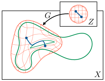
Figure 3: Real data manifold (green) vs. the generator manifold (red dashed), where linear coordinates in $Z$ result in nonlinear coordinates in $X$. Blue line shows a linear interpolation in the latent space mapped to the sample space.

4 An adaptive metric for generative
adversarial networks

The goal of generative modeling is to match the generated distribution $p_{G}$ in (1) with the data distribution $p_{X}$. Assuming that there is no mismatch between the generator image and the data manifold, it must hold for the deterministic GAN approach that,

$$p_{X}({\bf x}) =p_{G}({\bf x})$$ (7)

$$=\int_{{\bf z}\in Z}\delta({\bf x}-G({\bf z}))p_{Z}({\bf z})d{\bf z}$$ (8)

$$=p_{Z}(G^{-1}({\bf x})),$$ (9)

for the pre-image of $G$, i.e., $G^{-1}({\bf x})=\{{\bf z}:G({\bf z})={\bf x}\}$. Since the generator $G$ is modeled as a (continuous) feed-forward network with a pre-determined architecture and a simplistic latent distribution where typically $d<D$, it cannot be guaranteed to find network parameters such that equations (7)–(9) hold in general. Also, since the data manifold is not known everywhere, but only in the sample points included in the finite-sized dataset, the (continuous) generator needs to extrapolate between the observed points on the data manifold; an estimation procedure that forms another source of manifold mismatch. One may distinguish between two types of mismatch; firstly when the generator synthesizes unrealistic data, then

$$\exists\,{\bf z}:G({\bf z})\notin X,$$ (10)

and, secondly, when the the generator cannot reach all points on the data manifold (mode collapse), then

$$\exists\,{\bf x}:\{{\bf z}:G({\bf z})={\bf x}\}=\varnothing.$$ (11)

An illustration of these two mismatches can be seen in Figure 3, where unrealistic generation happens at the hole in the manifold and outside of the green set on the left, while mode collapse occurs outside of the red dashed set on the right. The mode collapse mismatch is a common issue for GANs; and many approaches exist for circumventing it, see, e.g., [22] and the references therein for a good overview. This paper instead focuses on the first type of mismatch, were the generator synthesizes samples which are not in the (unknown) data manifold, i.e., being unrealistic, and describes an approach for circumventing it. To that end, consider the adapted curve length

$$L^{*}(\boldsymbol{\gamma})=\int_{t=a}^{b}\left\lVert\ \dot{\boldsymbol{\gamma}}(t)\right\rVert_{R^{*}}dt,$$ (12)

where the curve length is defined by a proposed metric, which is infinite outside the data manifold. For the Euclidean norm in sample space this is

$$\mathbf{M}^{*}_{{\bf z}} =\left\{\begin{array}[]{ll}\mathbf{J}_{{\bf z}}^{\top}\mathbf{J}_{{\bf z}}&G({\bf z})\in X\\ \infty\cdot{\bf I}&G({\bf z})\notin X\end{array}\right.,$$ (15)

such that the adapted norm is

$$\left\lVert\dot{{\bf z}}\right\rVert_{R^{*}} =\left\{\begin{array}[]{ll}\left\lVert\mathbf{J}_{{\bf z}}\dot{{\bf z}}\right\rVert_{2}&G({\bf z})\in X\\ \infty&G({\bf z})\notin X\end{array}\right.,$$ (18)

or equivalently,

$$\left\lVert\dot{{\bf z}}\right\rVert_{R^{*}} =\left\lVert\mathbf{J}_{{\bf z}}\dot{{\bf z}}\right\rVert_{2}+\phi({\bf z})$$ (19)

$$\phi({\bf z}) =\left\{\begin{array}[]{ll}0&G({\bf z})\in X\\ \infty&G({\bf z})\notin X\end{array}\right..$$ (22)

In this formulation, $\phi:Z\rightarrow\mathbb{R}$ is a penalty function such that any curve traversing points outside the data manifold has infinite length, ruling these out as shortest paths. However, calculating $\left\lVert\cdot\right\rVert_{R^{*}}$ requires knowledge of the data manifold beforehand, which is infeasible, and to that end, one may approximate $\phi$ using some auxiliary function. Depending on the deep generative modeling method, $\phi$ may be approximated in different ways, however always such that the function has small values for realistic data, and large values for unrealistic data. For GANs, a natural choice of auxiliary function would be based on the discriminator, $D:X\rightarrow\mathbb{R}$. In the origin work by Goodfellow et al., [11] the discriminator maps each data sample into the interval $(0,1)$ and its image $D({\bf x})$ on some ${\bf x}\in X$ is interpreted as the probabilty of ${\bf x}$ being a sample from the real data distribution $p_{X}$. So, to calculate shortest paths for a GAN, the auxiliary function may be approximated as

$$\phi({\bf z})\approx\frac{\lambda}{D(G({\bf z}))+\epsilon},$$ (23)

where $\lambda>0$ is a hyperparameter of the model, and $\epsilon~{}>~{}0$ a  small number added to ensure numerical stability when $D({\bf x})\approx 0$.

For computational reasons, the shortest path may be approximately calculated using a discretized version of ${\boldsymbol{\gamma}}(t)$. To that end, consider a sequence of $T+1$ points in the latent space along the curve ${\boldsymbol{\gamma}}$, i.e., ${\boldsymbol{\gamma}}(t_{i}),i=0,\dots,T$, such that ${\boldsymbol{\gamma}}(t_{0})={\boldsymbol{\gamma}}(0)$ and ${\boldsymbol{\gamma}}(t_{T})={\boldsymbol{\gamma}}(1)$. In sample space, this sequence forms a corresponding discrete path $(G\circ{\boldsymbol{\gamma}})(t_{i}),i=0,\dots,T$, for which the discrete analogue of the energy functional for the proposed metric becomes

$$E^{*}_{t_{i}}({\boldsymbol{\gamma}})=\sum_{i=1}^{T}\frac{1}{T} \left\lVert(G\circ{\boldsymbol{\gamma}})(t_{i})-(G\circ{\boldsymbol{\gamma}})(t_{i-1})\right\rVert_{R^{*}}^{2},$$ (24)

which we approximate, using (23), by

$$E^{*}_{t_{i}}({\boldsymbol{\gamma}})\approx\sum_{i=1}^{T}\frac{1}{T} \bigg{(}\left\lVert(H\circ G\circ{\boldsymbol{\gamma}})(t_{i})-(H\circ G\circ{\boldsymbol{\gamma}})(t_{i-1})\right\rVert_{2}$$

$$+\lambda\Big{(}(D\circ G\circ{\boldsymbol{\gamma}})(t_{i})+\epsilon\Big{)}^{-1}\bigg{)}^{2}.$$ (25)

In order to find a geodesic between ${\boldsymbol{\gamma}}(0)$ and ${\boldsymbol{\gamma}}(1)$, we follow the approach of Yang et al. [32] to model the curve using a polynomial parametrization with trainable parameters $\psi$, for which the geodesic can be found by minimizing $E^{*}_{t_{i}}({\boldsymbol{\gamma}}_{\psi})$ over $\psi$ via gradient descent or its variants applied on the discretized objective from (4).

Adapting our method to Wasserstein GANs. In order to reuse pre-trained models of high quality generators, we aim to apply the proposed method to Wasserstein GANs, where the discriminator is usually called the critic; a terminology adopted herein. The change from discriminator to critic requires some adjustments of our method. A distinguishing difference of Wasserstein GANs to regular GANs is to replace the $(0,1)$-valued discriminator by one that can assign an arbitrary real number. The task of assigning high values to real and low values to generated samples remains unchanged, and a Lipschitz constraint on the discriminator prevents the divergence of their mean difference. With (23) relying on the assumption of a $(0,1)$-valued discriminator, but this not holding for the critic, we normalize critic values to $(0.1)$ using an approximate maximum and minimum critic value determined from generated samples. A more difficult issue is the lack of well-defined bounds and, more generally, that critic values cannot be interpreted as a probability of the sample being real. While the critic of a WGAN provides gradient information between real and generated samples toward improved equality, it is possible that non-realistic samples attain high critic values, for example if they fall outside the convex hull of real and generated samples. Figure 4 shows such an example of a real and generated data distribution and a theoretically optimal Wasserstein GAN critic, where the highest critic values are found off the real manifold. (The optimality of the displayed critic follows from [30, Theorem 5.10], and Observation 4 in [24] provides another illustration where an optimal critic assigns a higher critic value to a generated sample than a real). Therefore, caution is advised when enforcing high critic values, but since our main motivation is to improve the quality of images close to a shortest path, useful gradient information is all we need.

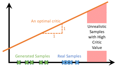
Figure 4: Values of optimal Wasserstein critics do not correspond to realisticness, but the gradient information is useful

5 Experiments

Our experiments compare the following list of interpolation methods: (a) Linear - Linear interpolations in latent space, which are mapped by the generator $G$ onto the image manifold. (b) sqDiff - Shortest path on the image manifold measured with the Euclidean metric in sample space; i.e., the minimum of (6) with $H$ being the identity function. This minimizes squared differences of images under $G$ and is a method proposed in [2, 8, 27]. (c) sqDiff+D - A herein proposed method using (4), where the metric combines sqDiff with enforcing high discriminator values. (d) VGG - Shortest path on the image manifold as measured by a weighted Euclidean distance between features in different layers of the VGG network (as detailed in [19]). VGG+D - A herein proposed method combining the method by Laine [19] with enforcing high discriminator values; i.e., (4) with $H$ being feature maps of the VGG network. (f) Linear in sample space - As a comparison to sqDiff we show the shortest path in sample space with respect to its Euclidean metric, which is a straight line. This path is independent of the generator function, illustrating a completely naive interpolation.

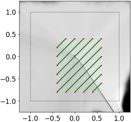
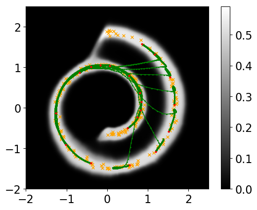
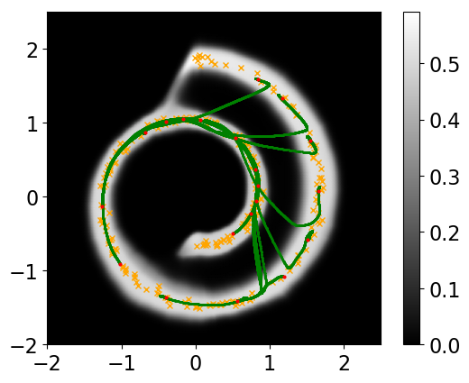
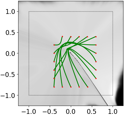
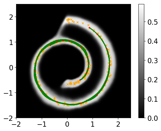
Figure 5: Comparison of interpolation paths (green) in latent space (left) sample space (right) for swiss roll; Top to bottom: (a) Linear, (b) sqDiff, and (c) sqDiff+D (proposed).

For each of the methods sqDiff, sqDiff+D, VGG and VGG+D, we parametrize a path using a multi-dimensional polynomial with fixed endpoints by specifying the coefficients of the constant and the linear part. The coefficients to higher order terms are learned by minimizing the respective objectives. For a fair comparison, all methods are trained for the same number of epochs. We find that all methods benefit from ”early stopping”, i.e., not training until convergence. This is theoretically justified above for methods using a Wasserstein critic, but we also find that the bias toward blurry images of sqDiff and VGG (explained below) becomes more severe with more training iterations. We describe all hyperparameter settings and implementation details in Appendix A. Our code is published under https://github.com/petzkahe/progan_geodesics.

5.1 Swiss roll

As a proof of principle, we consider the two-dimensional toy dataset of the so-called swiss roll. We trained a GAN with a two-dimensional latent space and visualized both generated samples (in green) and discriminator values (grayscale background) in Figure 2 on page 2. By sampling from a dense grid in latent space, we can visualize how the GAN maps the two-dimensional latent space onto the swiss roll. At the end of training, generated samples stay on the swiss roll with high probability. Still, a low density of samples do fall off the swiss roll, implying large gradients of the generator at the corresponding latent points ${\bf z}$, resulting in large metric $\mathbf{M}_{\bf z}$. Nonetheless, geodesics with respect to the method sqDiff traverse this region of unrealistic samples if the resulting path is shorter in the sample space $\mathbb{R}^{2}$. Figure 5 compares paths obtained from Linear, sqDiff and sqDiff+D. sqDiff results in paths in sample space that are more smooth than the paths of Linear, but, as predicted, will often fall off the swiss roll. Taking the discriminator information into consideration, our proposed method sqDiff+D avoids regions of predicted fake samples and is therefore able to find smooth paths following the swiss roll.

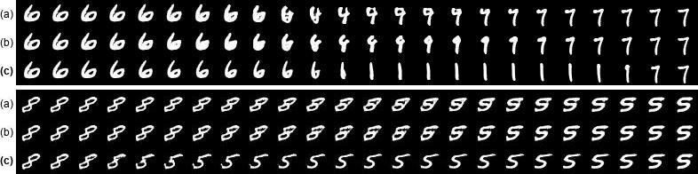
Figure 6: (a) Linear, (b) sqDiff and (c) sqDiff+D (ours) on MNIST showing our method to find a realistic smooth path.

5.2 MNIST

In a typical next step, we apply our method to the MNIST dataset [20]. Due to the discrete classes of digits, it seems debatable how a direct path between digits should look. The method sqDiff is expected to smoothly traverse through non-realistic samples, whereas Linear may traverse many digits on a lengthy path. Figure 6 shows that our method sqDiff+D is able to find a short path of high quality with quick transitions between digits.

5.3 ProGAN on CelebA

We apply our proposed method to CelebA images [21] using the tensorflow implementation of ProGAN by Karras et al. [14]; a progressively grown Wasserstein GAN (see WGAN-GP [1, 12]). We download the pre-trained network and reuse it in all of our experiments. As a pre-processing step, we set the feature map used for Minibatch Distcrimination (see [13]) to zero , which is necessary to obtain well-defined critic values, independent of the batch statistics. Then, as the Wasserstein critic is not limited to $(0,1]$, we sample a large number of points in the latent space, for which we evaluate the critic values and make note of the range of values. In subsequent evaluations, all critic values are scaled by this range in order to obtain values in $(0,1]$, as used in the proposed loss.

An evaluation of the pre-trained critic. Our method assumes a critic that is able to differentiate the quality of generated samples. Figure 7 (a) shows a histogram of critic values on generated (fake) and real samples for the critic trained in [14]. The significant overlap is a proof of the WGAN objective to be at an equilibrium. However, random samples (shown in Appendix B.1.1) show that, despite the high quality of samples, it is still often easy for a human to tell real apart from generated samples, which ideally should be detected by the critic network. To find the relevant gradient information, we fine-tune the provided networks. We deviate from an equal learning rate for critic and generator network to a learning rate of $5*10^{-4}$ for the critic and a learning rate of $10^{-4}$ for the generator, allowing the critic to gradually improve in comparison to the generator, but without worsening the generator results (We also experimented with training the discriminator only, but found the problem of observing high critic values for unrealistic samples as discussed above to worsen under this training regime. At the same time, maintaining a positive, but small, learning rate for the generator kept the generating close to constant.) We pick a model after training on 70k images ($<6~{}{\%}$ additional training). Figure 7 (b) shows the histogram of real and generated samples for this critic, which shows that the new critic has some understanding of differentiating real and fake.

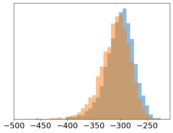
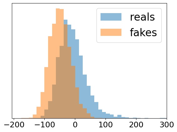
Figure 7: Histogram of critic values over each 5000 real (blue) and 5000 generated/fake (orange) samples. Left: ProGAN from [14]. Right: Our fine-tuned ProGAN

The necessity to fine-tune a critic before the application of our method could in principle be circumvented by training the ProGAN from scratch with an adapted training schedule. Otherwise, as in our case, the extra training is negligible in comparison to the training time of the provided model.

Comparison of the linear and proposed methods. Randomly sampling points from the generator often gives images that can be easily distinguished from real samples (see B.1.1). As a result, the linear interpolation shows several artifacts from generation. If, however, two generated samples of high quality are observed, then we find that the linear interpolation in latent space often results in curves of high quality images, a fact that has been previously observed by Chen et al. in [8]. We distinguish three scenarios for comparison of our proposed method to the linear interpolation in latent space: (i) Linear interpolation in sample space results in images of low quality, as shown in Figure 9. In this case, our method is able to find a much better path of high quality. (ii) Linear interpolation shows samples of high quality, but the path is not a direct path, as shown in Figure 10 (left). In this case, our method finds a more direct path of similarly high quality. (iii) Linear interpolation gives a direct path of high quality, as shown in Figure 10 (right). In this case, our method does not change the path and approximately agrees with the linear method.

Comparison of sqDiff and VGG with the proposed methods. We find that both sqDiff and VGG both work well in finding a short and direct path, which can help to avoid bad regions crossed by Linear. However, we find that both methods often result in blurry images with VGG slightly outperforming sqDiff. Despite a shorter path, this often results in paths of lower image quality than linear interpolation in latent space, see Figure 9 and 10 (left). Our method additionally enforces high discriminator values. It thereby follows the short paths obtained from these methods, but results in higher quality samples with images that are more crisp. Figure 11 shows critic values along the curve of Figure 9 (left) as well as averaged critic values over several paths. Reflecting visual analysis, the linear method usually obtains higher critic values than both sqDiff and VGG, but our method improves the poor image quality of the shortest path by realizing higher critic values close by.

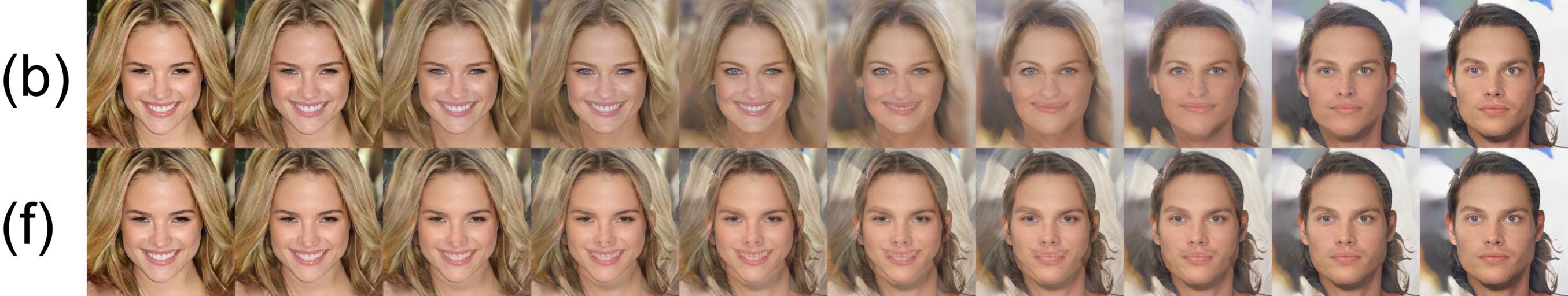
Figure 8: sqDiff approximates linear interpolation in sample space on the image manifold, resulting in blurry images that our proposed method can improve upon.

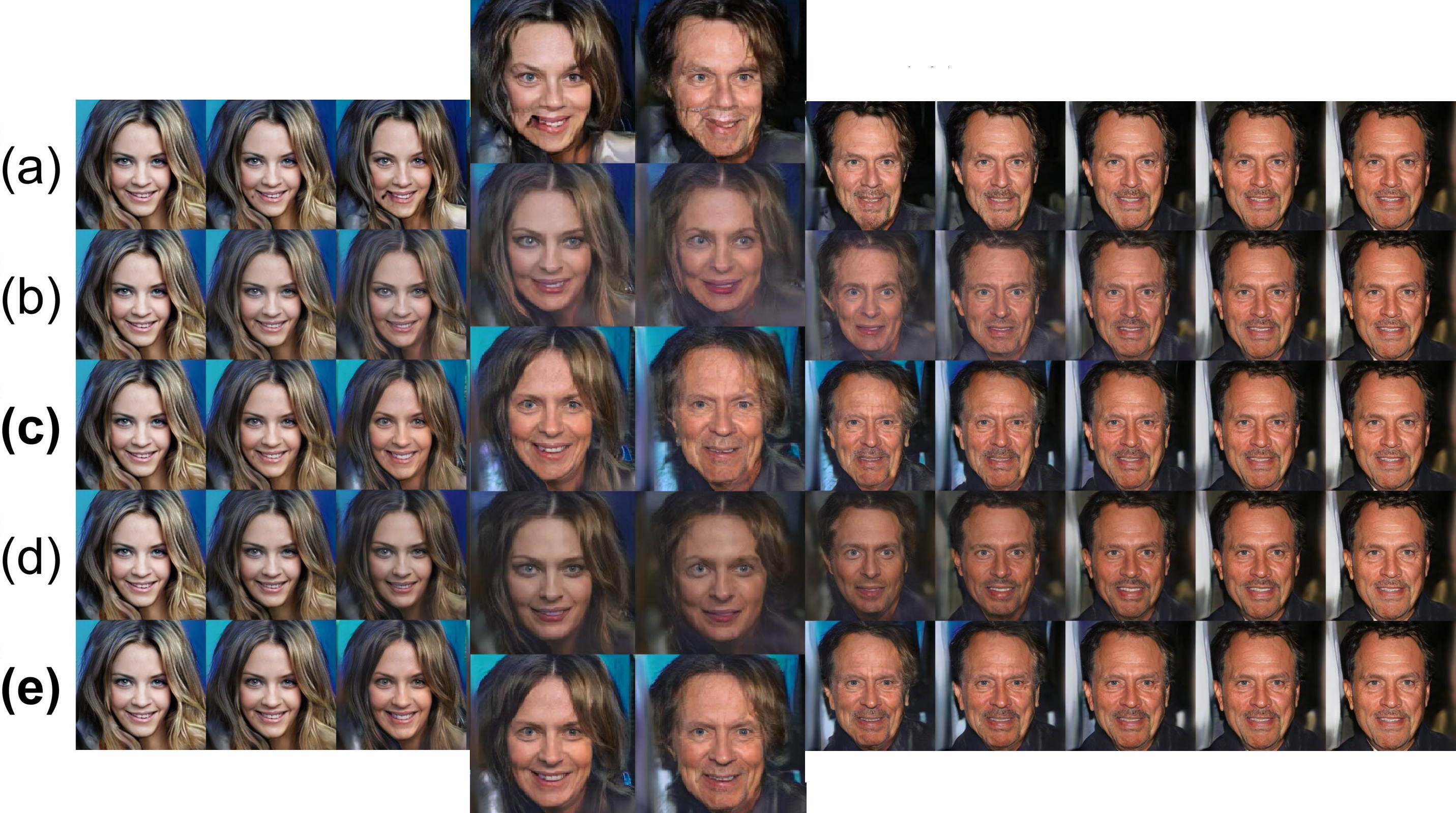
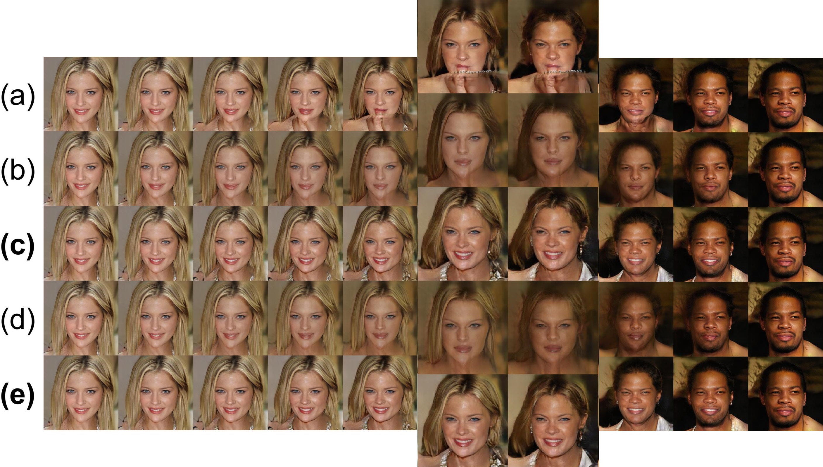
Figure 9: Comparison of (a) Linear, (b) sqDiff, (c) sqDiff+D, (d) VGG and (e) VGG+D. Linear falls off the real data manifold and sqDiff and VGG result in blurry images of low quality. Our proposed methods recover crisp images from the short paths of sqDiff and VGG resulting in a interpolating path of high quality images.

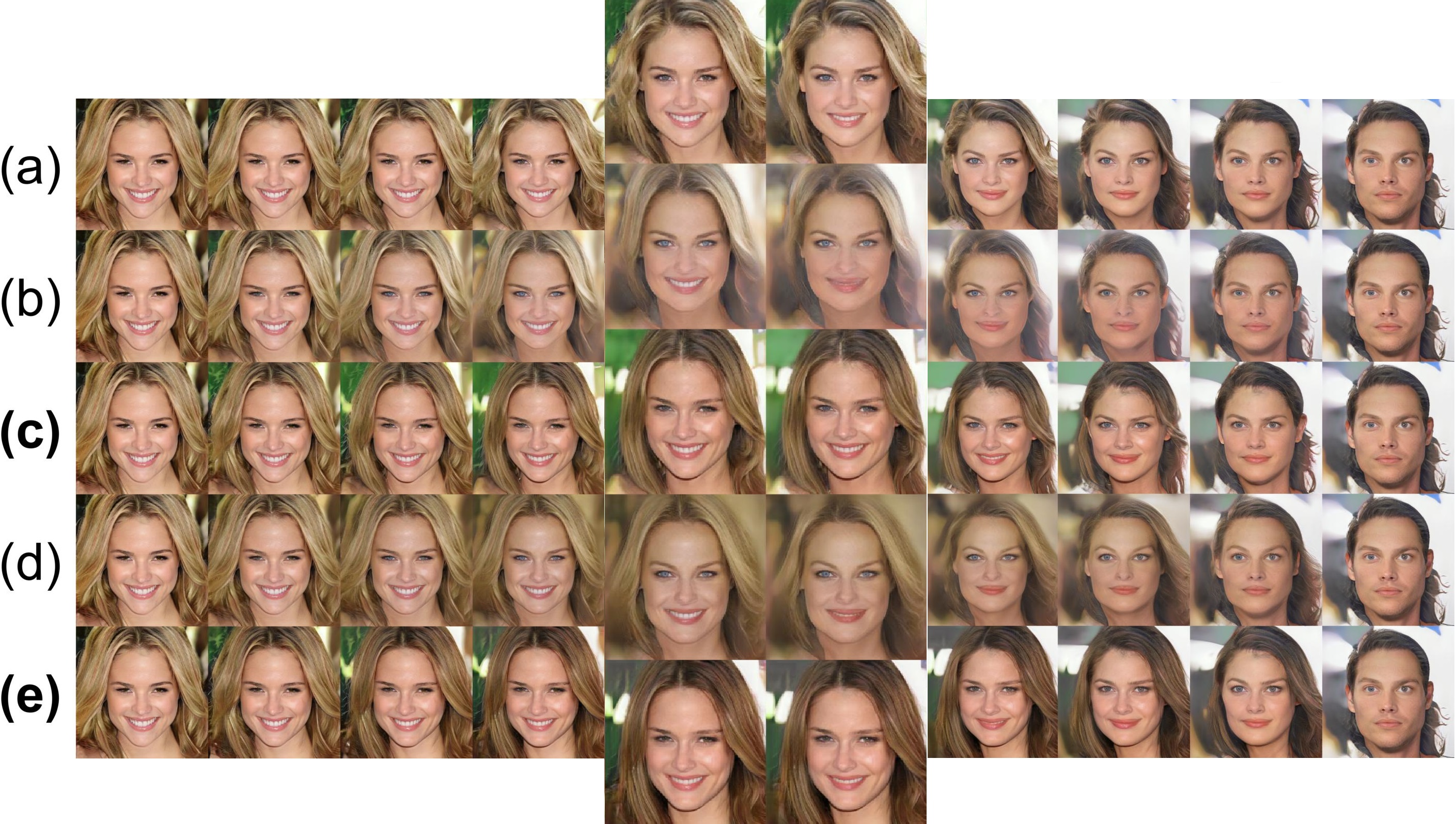
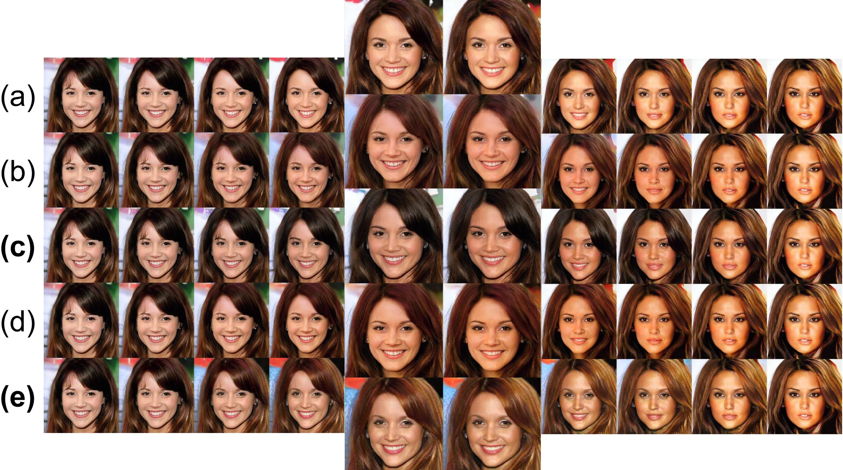
Figure 10: Comparison of (a) Linear, (b) sqDiff, (c) sqDiff+D, (d) VGG and (e) VGG+D. Quality of Linear is good and (left) not close to the short path dqDiff so that sqDiff+D and VGG+D recover from blurry images from sqDiff and VGG resp., or (right) close to an expected geodesic on the image manifold, in which case all methods approximately agree.

We explain the blurriness observed in both sqDiff and VGG by a curve that follows the requested objective too closely. Suppose the generator would be capable of producing any image in the sample space, then the closest path according to sqDiff would be linear interpolation in sample space, which results in a blurry path as visualized in comparison in Figure 8. The trained generator is expected to generate real-looking faces from anywhere in latent space, so we cannot find this curve exactly, but due to a mismatch of manifolds of real and generated images, similar paths can be found. Linear interpolation in feature spaces of the VGG network improve upon this, but some blurriness remains.

Limitations The success of the proposed method relies on discriminator (or critic) values that can distinguish samples of good quality from samples with poor quality. For the swiss roll, the good performance of the discriminator can be seen from the background color in Figure 6. For the other datasets, we find that the discriminator is not always reliable on single images, discovering a peculiar property of the trained critic. By evaluating the critic on small perturbations in the latent space, the critic values cover a large part critic’s range without a significant visual change of the generated image. We showcase this phenomenon in Figure 17 in Appendix B.1.4 for the CelebA dataset.

The reasons are potentially twofold: For one, a general property of Lipschitz-1 functions from a high-dimensional space of dimension $D$ (here $D=3\cdot 1024^{2}$) to a one-dimensional space is that small changes of size $\epsilon$ to all input dimensions can change the output by $\sqrt{(}D)\epsilon$. Here, to cover a range of $100$ in critic value, a change of all pixels by $0.0564$ can be sufficient. Secondly, the use of minibatch discrimination may disrupt the correlation between critic value and subjective realisticness, both locally and globally. For consistently penalizing the realisticness of shortest paths, we remove the minibatch standard deviation feature map. But the relative ordering of samples may still not correspond to image quality.

The observation implies that regions of poor image quality can not always be avoided on the CelebA dataset by enforcing high critic values. Indeed, we find that the proposed method can not always recover from poor image quality along the interpolating curves. However, we still find VGG+D outperforms all competing methods resulting in paths that are always at least as good as the interpolations found with the other methods. In particular, enforcing high critic values escapes blurry regions traversed by methods sqDiff and VGG.

Further, we note that some care must be taken in selecting and fine-tuning the critic network to prevent biased interpolations. By only fine-tuning the pre-trained ProGAN’s critic network, we found a critic that it favored bright lightening conditions. As a direct consequence, our method became biased toward white people and appeared to suffer from the overshooting problem discussed above, converging to extremely bright samples (see B.1.3).

Summary of results. Taken together, we find that our proposed method is always as least as good as linear interpolation in sample space, but can improve upon it in case of failure. While the competing methods sqDiff and VGG alone result in direct paths between two endpoints, they result in blurry images. Our method proposes to exploit gradient information from the critic network, enabling us to find direct paths of higher quality.

6 Discussion and Conclusion

At a theoretical equilibrium of a GAN objective, there is no gradient information from the discriminator between generated and real images. If the generator optimally matches the true data distribution, then the lack of discriminator information reduces the proposed methods to sqDiff and VGG respectively. As a result, our method is only interesting for imperfect generators that do not match the true data distribution, which is the practical case for state-of-the-art GANs. For such a generator, our results show that the discriminator information can be used to improve the sample quality of interpolatiog curves. Further improvements with the proposed method can be expected using a tailored training schedules for GANs to produce strong discriminators in the setting of sparse realistic datasets.

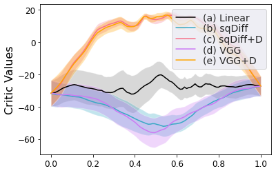
Figure 11: Critic values along paths. Left: Mean $\pm 1$ standard error of mean (12 paths). Right: Paths of Figure 9 left.

To conclude, we have presented a method for incorporating both networks of a GAN into a method for learning realistic interpolations on the generator’s image manifold. The proposed method is lightweight as it is post-hoc; reusing the discriminator that is learned in parallel to the generator. Incorporating discriminator values together with meaningful distances in a metric can avoid regions where the generator image and real data distribution do not align, resulting in paths that stay on the real data manifold. In its essence, high quality paths were achieved by discriminating against unrealistic samples.

Swiss roll		MNIST		CelebA-HQ
D	self-trained	D	trained using [14]	D	fine-tuned from [14]
n_interp_pts	1024	n_interp_pts	24	n_interp_pts	10
poly_degree	6	poly_degree	4	poly_degree	3
n_train_steps	1000	n_train_steps	100	n_train_steps	300
learn_rate	$10^{-3}$	learn_rate	$10^{-3}$	learn_rate	$10^{-3}$
hyperparam $\lambda$	$50$	hyperparam $\lambda$	$0.6$	hyperparam $\lambda$	$0.4$
coefficient_init	$10^{-1}$	coefficient_init	$10^{-4}$	coefficient_init	$10^{-4}$

LSUN Cars		LSUN bedrooms
D	fine-tuned from [14]	D	fine-tuned from [14]
n_interp_pts	10	n_interp_pts	10
poly_degree	3	poly_degree	3
n_train_steps	300	n_train_steps	200
learn_rate	$10^{-3}$	learn_rate	$10^{-3}$
hyperparam $\lambda$	$0.2$	hyperparam $\lambda$	0.2
coefficient_init	$10^{-4}$	coefficient_init	$10^{-4}$

Appendix A Training setup

A.1 Polynomial parametrization

To find shortest paths, i.e., geodesics, with respect to the different metrics, we parametrize a multi-dimensional polynomial

$$p(t)=a_{0}+a_{1}t+a_{2}t^{2}...+a_{n}t^{n},$$

where each $a_{i}\in\mathbb{R}^{d}$ for $d$ the dimension of the latent space. When learning shortest paths by minimizing curve lengths over the polynomial coefficients $a_{i}$, we do not want the start and endpoint to change. To that end, we consider coefficients $a_{i},i\geq 2$ as free parameters and calculate the constant part $a_{0}$ and the linear part $a_{1}$ to satisfy the constraints at the endpoint.

The standard choice for the parametrization of curves chooses a time-interval of $t\in[0,1]$. For higher degrees $j$ of polynomials, small numbers for $t$ result in vanishing contributions $a_{j}t^{j}$. To mitigate this problem, we parametrize all curves using the interval $t\in[1,2]$ instead.

A.2 Parameters of implementation

Our implementation allows the selection of several parameters for learning interpolating curves. The following list comprises the most relevant parameters

• D; The discriminator model to use for methods sqDiff+D and VGG+D.

• Start, End; Seeds for start and endpoint of the path.

• n_interp_pts; The number of interpolating points on the curve

• poly_degree; The polynomial degree of the interpolating curve

• n_train_steps; The number of training steps to update the curve parameters using Adam optimizer to minimize the respective objectives for path minimization with respect to the different metrics

• learn_rate; The learning rate used for the Adam optimizer minimizing path length.

• hyperparam $\lambda$; Hyperparameter used for strength of regularization of the curves using discriminator values as in (4) divided by dimension of image space of $H$.

• coefficient_init; Initialization of polynomial coefficients to learn is chosen uniformly random in the interval of this size

• Methods;Choice of method to use. Our implementation features linear interpolation, sqDiff, sqDiff+D, VGG, VGG+D, Linear interpolation in sample space and looking for high discriminator values only.

For each dataset, we manually searched for suitable hyperparameters based on visual exploration, Once we found a good setting, we used that choice of hyperparameters for the generation of all results.

Differences in hyperarameter settings between Swiss Roll versus MNIST and CelebA-HQ can be explained by using a regular GAN with $(0,1)$-valued discriminator for the swiss roll, while using a Wasserstein GAN for the other experiments (see Section 4, Adapting our method to Wasserstein GANs.

A.3 More implementation details

A.3.1 Swiss Roll

Examining the discriminator values for the GAN trained on Swiss roll in Figure 5, one sees that there is a thin black region of low values between the origin and the south-east corner. Following the, e.g., linear, paths crossing over this region one sees (in sample space) that these paths fall off the swiss roll’s real data manifold, by jumping across the roll instead of following along it. When training the GAN, this bad region of latent points is apparently not removed, but instead shrunk, becoming very very thin. Nonetheless, when interpolating across it, the results are detrimental. During training of sqDiff and the proposed sqDiff+D, we found that, starting from linear interpolation, there was not always enough gradient information available to escape the unrealistic path. Instead, we trained an ensamble of paths, having the same endpoints but different (and larger) initialization, where after training the path with smallest objective was chosen. In addition, because the bad region of latent points was so thin, to make the selection of hyperparameter less important, we replaced the discrete discriminator values along the paths by the geometric average of discriminator values between adjacent points, thus widening and flattening the region somewhat.

Appendix B Additional Experiments

B.1 CelebA-HQ

B.1.1 A grid of samples

In Figure 12, we examine a set of synthetic CelebA-HQ images (from our fine-tuned ProGAN) and corresponding critic values, sampled using latent codes drawn from $p_{Z}$, i.e., randomly from the generator manifold. It is apparently clear that many images are very realistic, meaning that they would fool a human examiner, but that a surprising amount (perhaps 20 % in this set) are still quite unrealistic, exhibiting either unnatural facial distortions, or show a varying amount of artifacts in either the foreground or in the background, which wouldn’t fool the human examiner. Indeed, to sucessfully utilize this generator in real-world applications, some points in the latent space will need to be avoided.

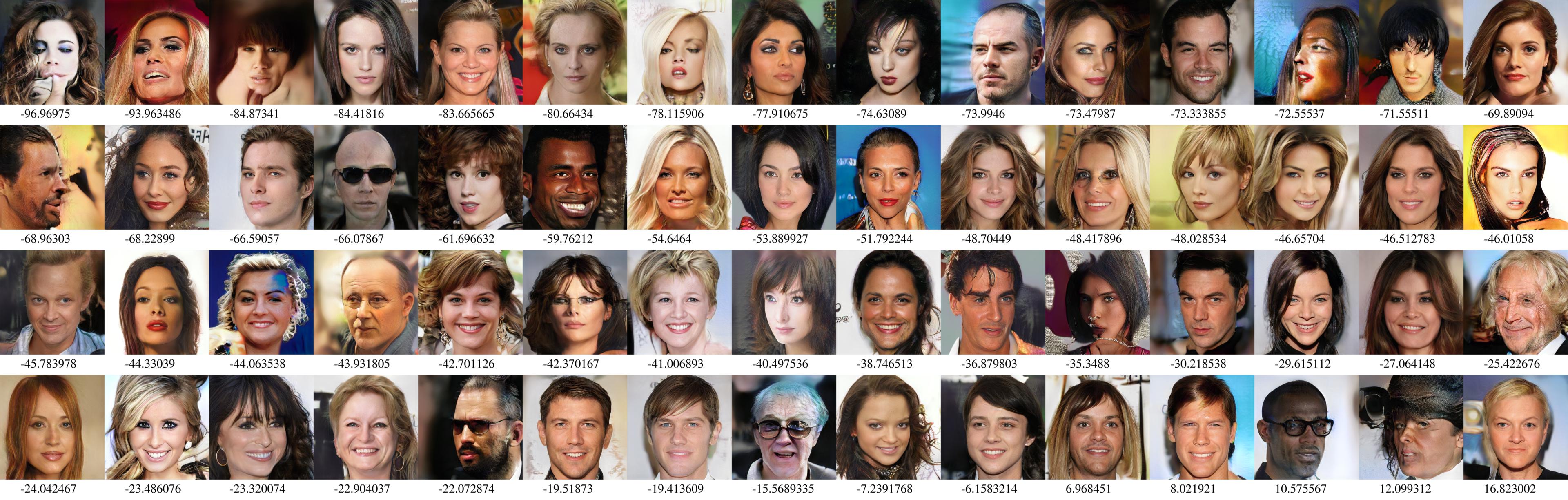
Figure 12: Randomly generated CelebA-HQ images using ProGAN.

To that end, figures 13 and 14 showcase the discriminator’s ability to separate the most realistic from the least realistic generations, by displaying a set of images with low and high discriminator values, respectively. These images form the two tails of the discriminator value distribution, sampled from a collection of 20k generated images. Considering the number of unrealistic examples in each set, they are not all and none, unfortunately, but they are in majority among the worst, and in clear minority among the best.

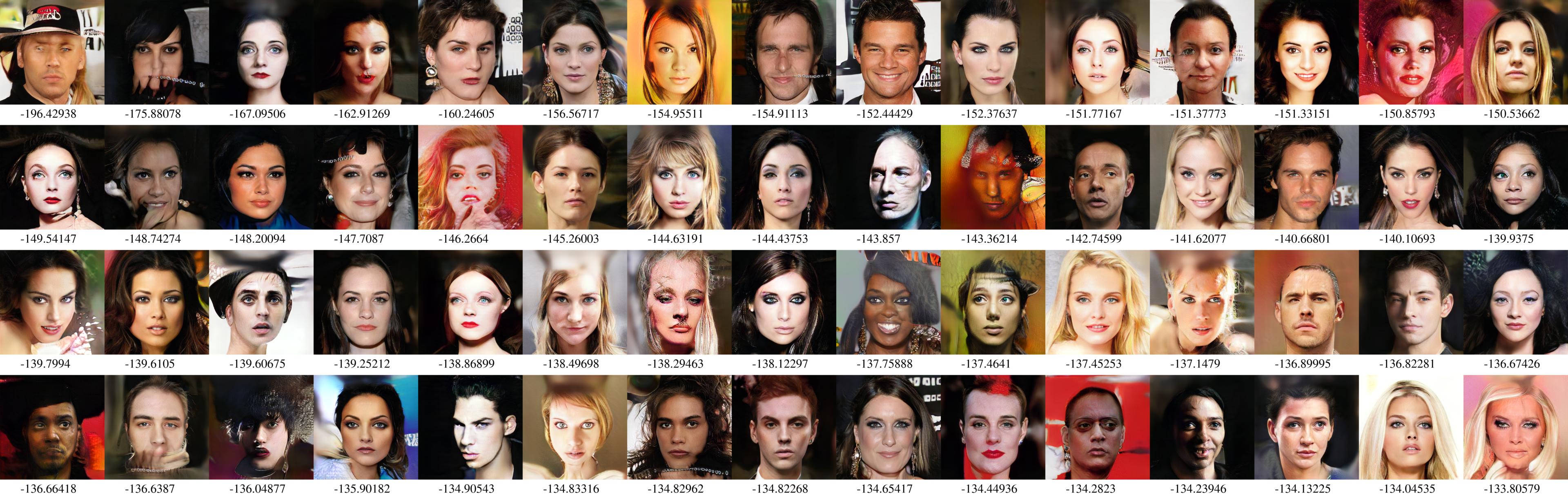
Figure 13: Worst-case images (among 20k random samples) according to our fine-tuned ProGAN discriminator network.

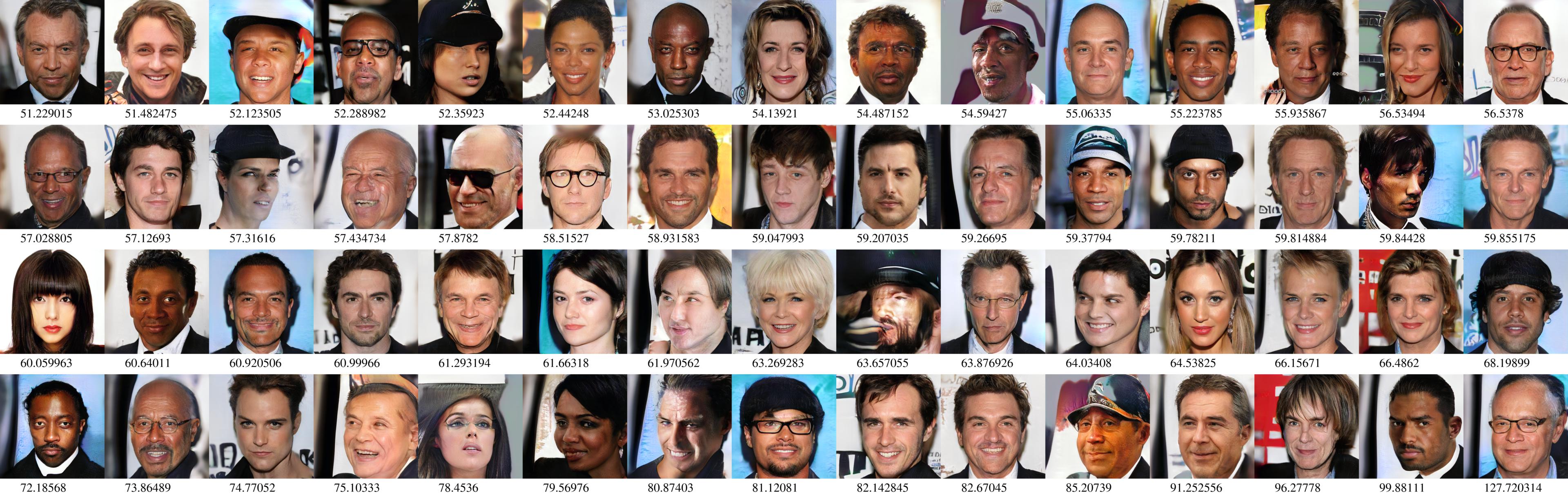
Figure 14: Best-case images (among 20k random samples) according to our fine-tuned ProGAN discriminator network.

B.1.2 Additional geodesics

Below follows some more examples of trained paths for ProGAN trained on CelebA-HQ for (a) Linear, (b) sqDiff, (c) sqDiff+D, (d) VGG and (e) VGG+D on CelebA.

Squared differences along paths

We show mean squared differences $\left|\left|G(\gamma(t_{i+1}))-G(\gamma(t_{i}))\right|\right|^{2}_{2}$ along 100 interpolation points for the twelve geodesics used for Figure 11, confirming that those are minimized for the method sqDiff. Similarly, VGG leads to small squared differences in image space, explaining the perceived blurriness. While Linear leads to large squared differences along the geodesic, our proposed methods sqDiff+D and VGG+D result in shorter paths (as measured by the squared differences in sample space). We explain the short distances close to the endpoints by the fact that, in the implementation of [14], latent vectors are projected onto a $512$-dimensional sphere of radius $\sqrt{512}$ before an application of the generator, so that larger distances on the sphere in latent space appear when coordinates cross the zero point.

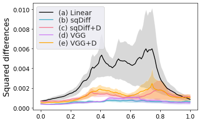
Figure 15: Squared Differences along paths. Mean $\pm 1$ standard error of mean (12 paths - the same paths as were used in Figure 11). The proposed methods sqDiff+D and VGG+D fall between the shortest possible path found by sqDiff and the Linear method.

Squared VGG feature differences along paths

We show squared feature differences of the VGG19 network as a measure of distance covered along paths. Following [19], we consider a weighted mean (by reciprocal of layer dimensions) of the layers conv_1_2,conv_2_2, conv_3_2, conv_4_2 and conv_5_2. We find that VGG minimizes this measure close to the endpoints, but obtains slightly larger values than sqDiff in the middle of the path. In general, sqDiff and VGG are similar in distance, confirming visual evaluation that both result in blurry paths. Apparently, the way to minmize $||H(G(\gamma(t_{i})))-H(G(\gamma(t_{i-1})))||$ in feature spaces defined by a continuous feature map $H$ is partially achieved by minimizing distances in image space $||G(\gamma(t_{i}))-G(\gamma(t_{i-1})||$, which is not entirely surprising. We also note that we do not train until convergence, which may explain the parts where VGG obtains slightly larger values than sqDiff. The comparison to the other curves is similar as above. Linear covers the largest distance, while the proposed methods sqDiff+D and VGG+D settle in the middle.

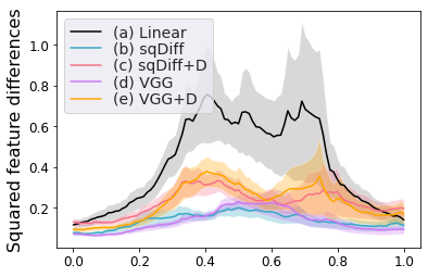
Figure 16: Squared Differences in VGG feature spaces along paths. Mean $\pm 1$ standard error of mean (12 paths - the same paths as were used in Figure 11).

B.1.3 Biased discriminators

Starting from the model trained by [14] and finetuning the discriminator only (on 2000 images) resulted in a critic that produced high quality images, but with a bias toward white people and bright illumination. All hyperparameter setting are unchanged from the images above in the following biased interpolations:

B.1.4 Local perturbations in latent space

Figure 17 shows generated samples and their critic values. Each row corresponds to images generated from small, local perturbations to the latent vector. While the generated samples do not change significantly, the critic values cover a large part of the range of the critic values. This showcases that critic values on single images may not always provide useful information for improvements of the sample quality.

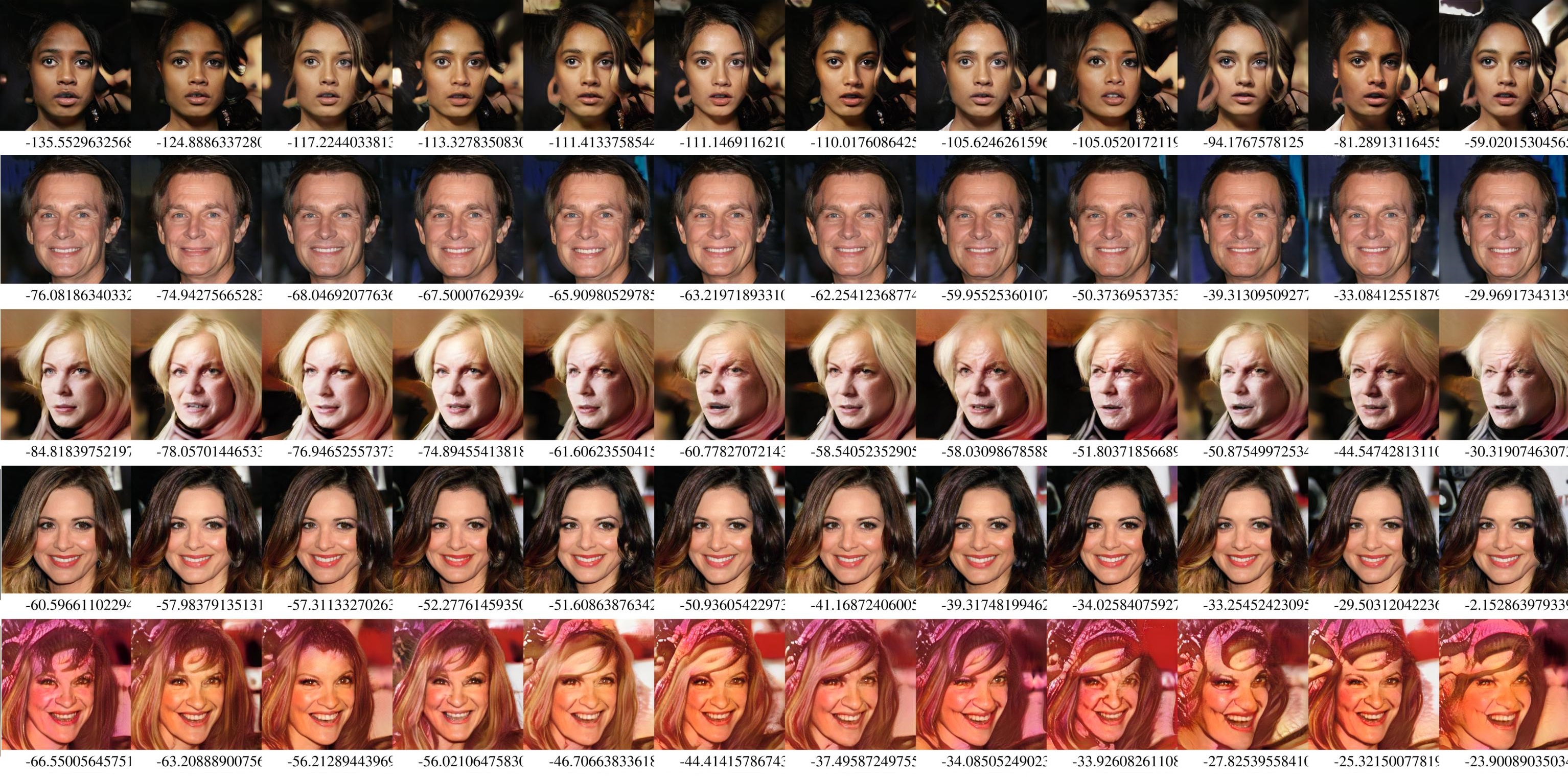
Figure 17: Critic values of ProGAN on generated images from small perturbations of a fixed latent vector. While the generated samples do not change significantly, the critic values cover a wide range.

B.2 MNIST

In the following figures, we illustrate some additional examples of trained paths for the ProGAN trained on MNIST using the same settings as above. Rows illustrate (a) Linear on top, (b) sqDiff in the middle, and (c) sqDiff+D at the bottom.

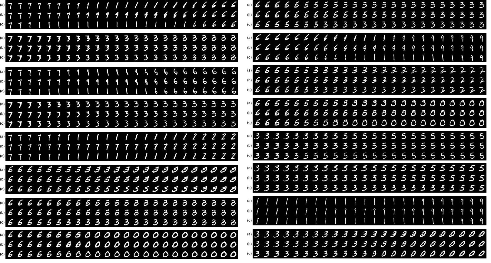
Figure 18: Comparison of (a) Linear, (b) sqDiff, and (c) sqDiff+D on MNIST.

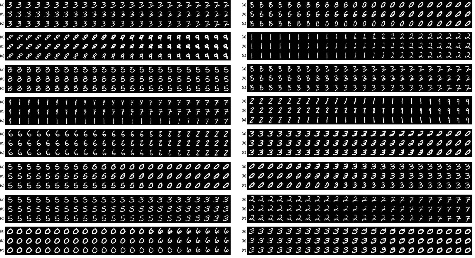
Figure 19: Comparison of (a) Linear, (b) sqDiff, and (c) sqDiff+D on MNIST.

B.3 LSUN-Cars

We additionally experimented on the LSUN-Car dataset. Both methods sqDiff and VGG to result in very blurry images on this dataset when trying to minimize the path length in sample space or VGG feature space. This is detrimental to our method that tries to improve upon the short path by incorporating critic values into the metric. We also found the Linear method to work well when the endpoints were chosen similarly, but otherwise linear fails to find a good interpolations. Whenever linear failed, we were not able to find short and realistic paths using the proposed method VGG+D, but the experiments show the possibility to improve the image quality significantly over VGG by using discriminator information. This functionality is demonstrated by the following two Figures, where the first choice of hyperparameter $\lambda$ balances shortest path and discriminator information, while the second puts emphasis on discriminator information leaving the shortest path significantly.

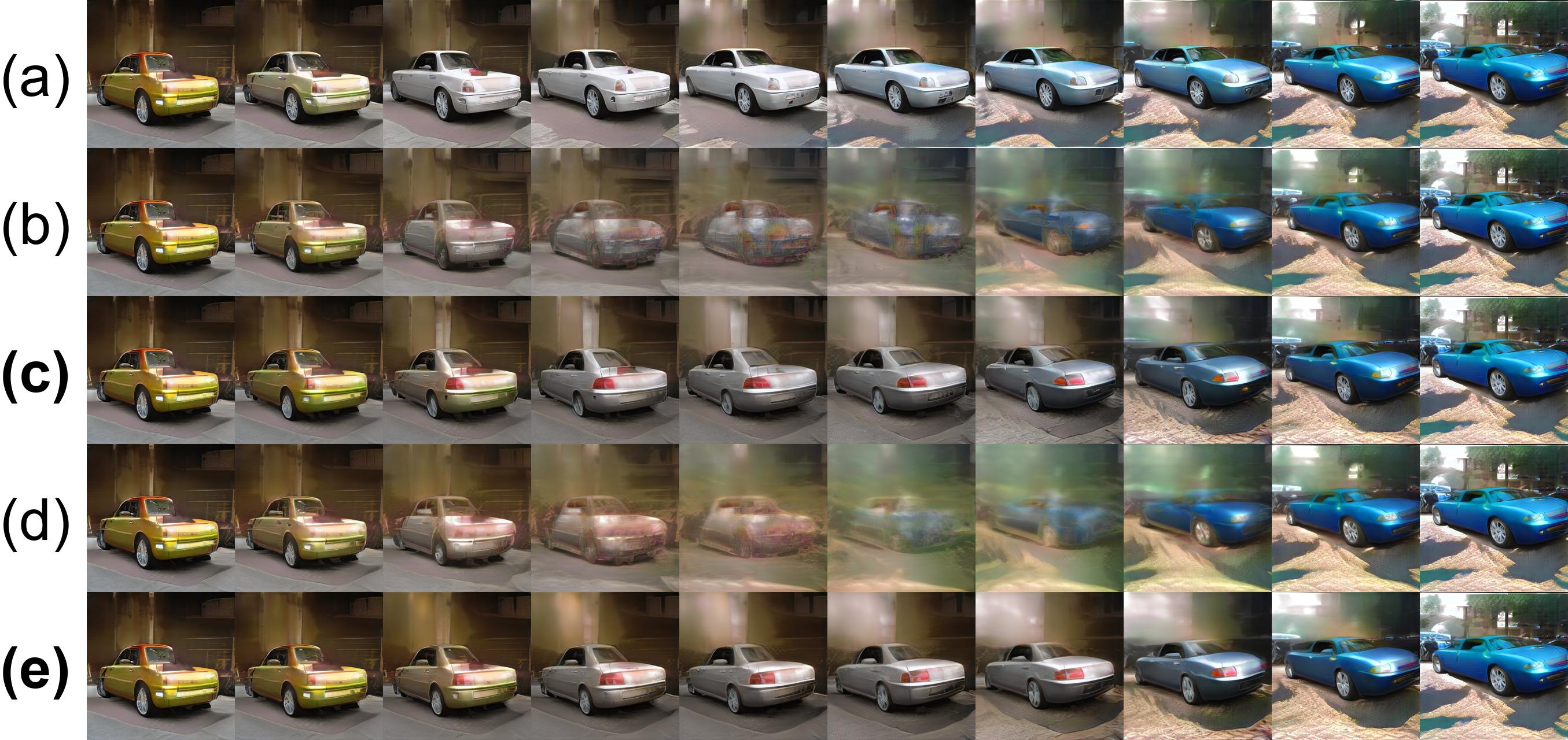
Figure 20: Comparison of (a) Linear, (b) sqDiff, (c) sqDiff+D, (d) VGG and (e) VGG+D on MNIST. sqDiff and VGG result in blurry images. Enforcing high discriminator in (c) and (e) improves image quality.

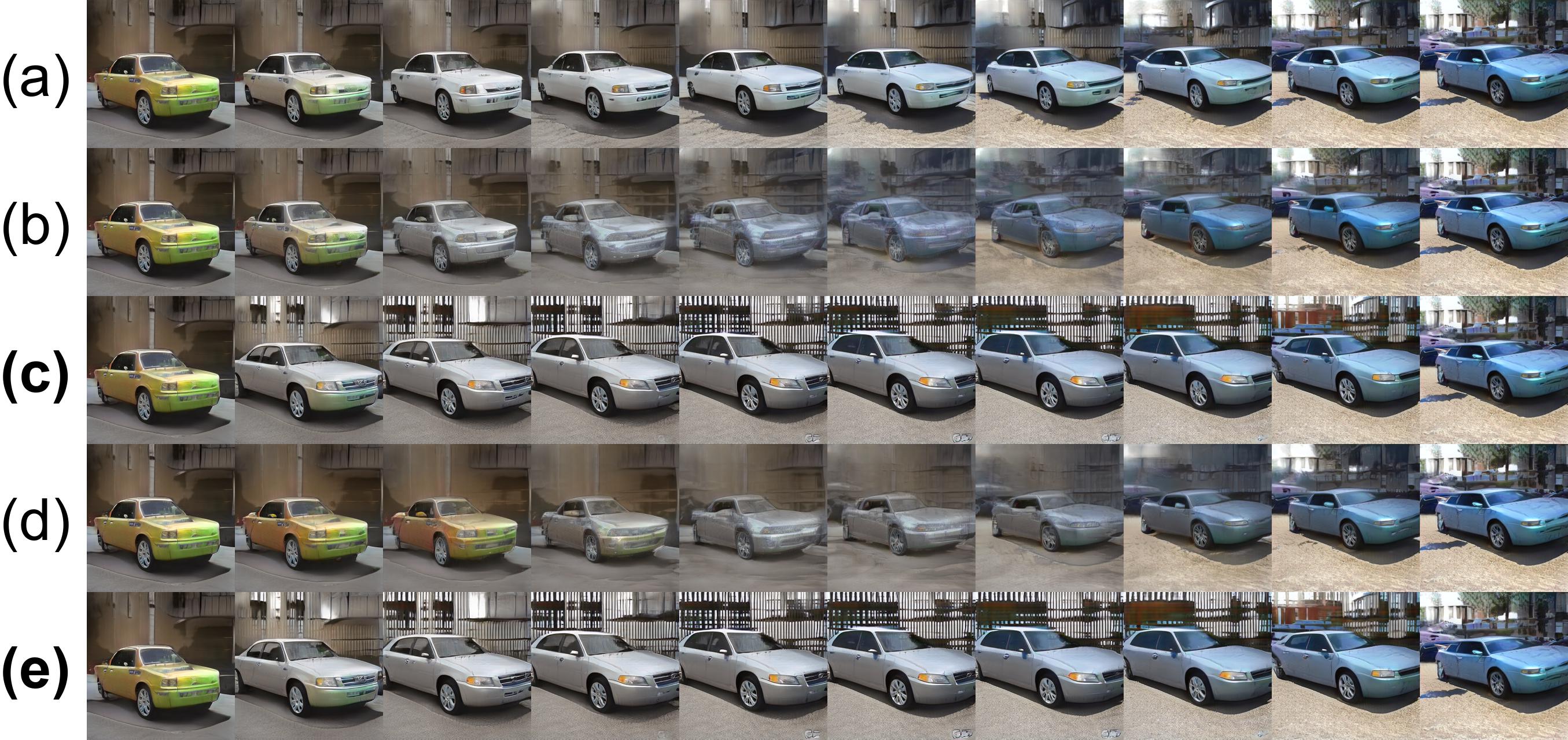
Figure 21: Comparison of (a) Linear, (b) sqDiff, (c) sqDiff+D, (d) VGG and (e) VGG+D on MNIST. The same endpoints as in Fig. 20, but with larger hyperparameter $\lambda$ putting more emphasis on high discriminator values than the objective to find shortest paths. While image quality improves, the path deviates from short paths significantly.

More examples comparing (a) Linear, (d) VGG and (e) VGG+D.

B.4 LSUN-Bedrooms

For the LSUN dataset of bedrooms, we exemplify here that our proposed method again recovers sharp images from blurry images along paths using VGG, and that the paths found by VGG+D can be more direct (see in particular the change of color in the third exaple).

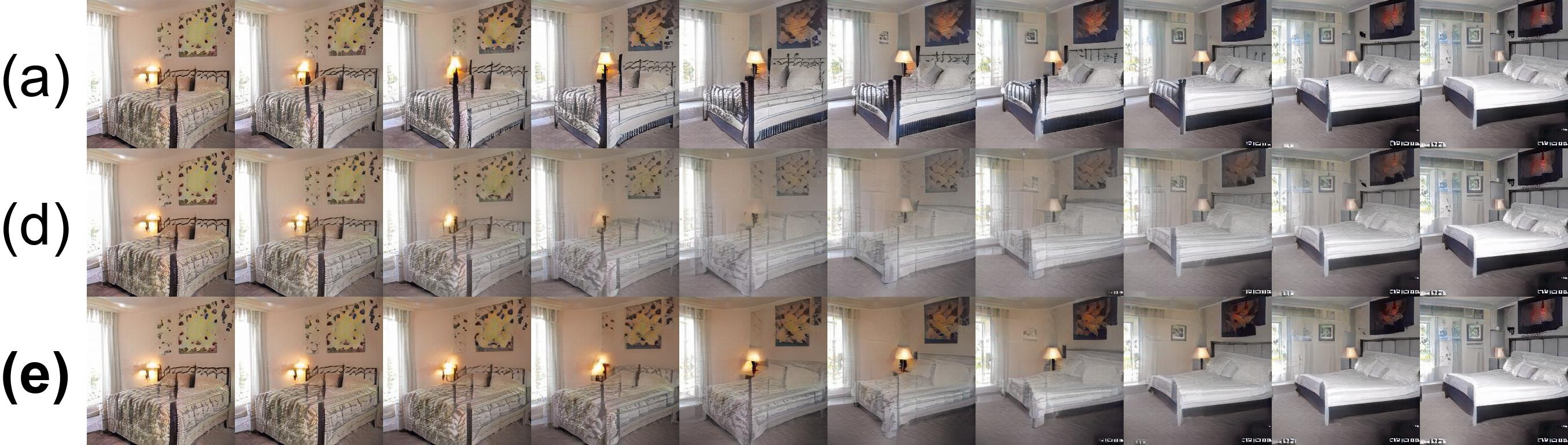
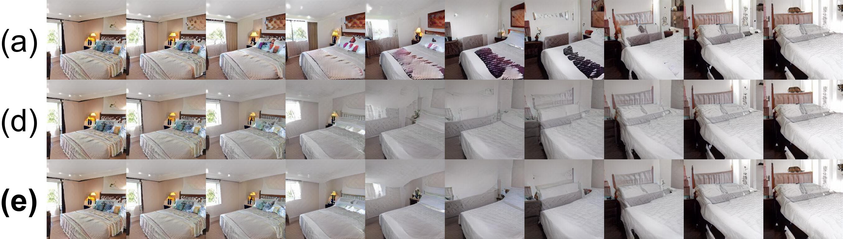
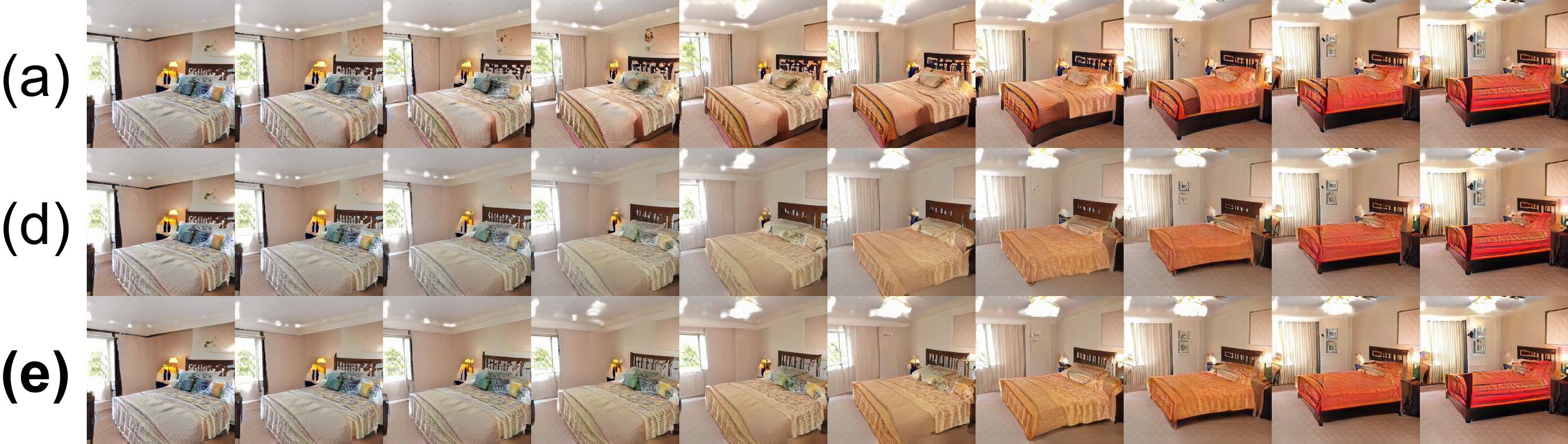
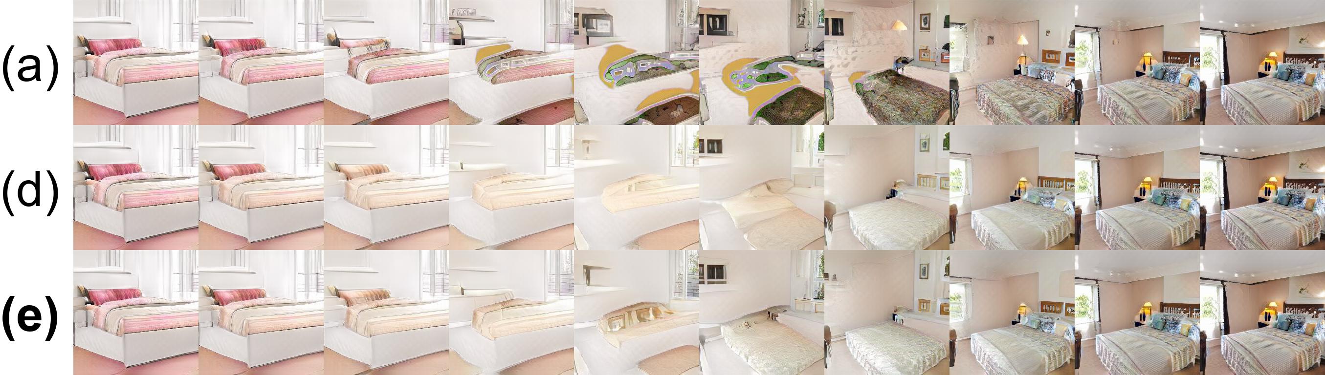
Figure 22: Comparison of (a) Linear, (d) VGG and the proposed method (e) VGG+D on LSUN-bedrooms.

References

- [1] Martin Arjovsky, Soumith Chintala, and Léon Bottou. Wasserstein generative adversarial networks. In Proceedings of the 34th International Conference on Machine Learning ICML, 2017.
- [2] Georgios Arvanitidis, Lars Kai Hansen, and Søren Hauberg. Latent space oddity: on the curvature of deep generative models. In Proceedings of the 6th International Conference on Learning Representations ICLR, 2018.
- [3] Georgios Arvanitidis, Søren Hauberg, and Bernhard Schölkopf. Geometrically enriched latent spaces. Proceedings of the 24th International Conference on Artificial Intelligence and Statistics, 2021.
- [4] Yoshua Bengio, Grégoire Mesnil, Yann Dauphin, and Salah Rifai. Better mixing via deep representations. In Proceedings of the 30th International Conference on Machine Learning, ICML, 2013.
- [5] David Berthelot*, Colin Raffel*, Aurko Roy, and Ian Goodfellow. Understanding and improving interpolation in autoencoders via an adversarial regularizer. In International Conference on Learning Representations, 2019.
- [6] Nutan Chen, Francesco Ferroni, Alexej Klushyn, Alexandros Paraschos, Justin Bayer, and Patrick van der Smagt. Fast approximate geodesics for deep generative models. In Artificial Neural Networks and Machine Learning ICANN: Deep Learning, 2019.
- [7] Nutan Chen, Alexej Klushyn, Francesco Ferroni, Justin Bayer, and Patrick van der Smagt. Learning flat latent manifolds with VAEs. Preprint arXiv:2002.04881, 2020.
- [8] Nutan Chen, Alexej Klushyn, Richard Kurle, Xueyan Jiang, Justin Bayer, and Patrick van der Smagt. Metrics for deep generative models. In International Conference on Artificial Intelligence and Statistics, AISTATS, 2018.
- [9] Xi Chen, Yan Duan, Rein Houthooft, John Schulman, Ilya Sutskever, and Pieter Abbeel. Infogan: Interpretable representation learning by information maximizing generative adversarial nets. In Advances in Neural Information Processing Systems 29 NeurIPS, 2016.
- [10] Manfredo P. do Carmo. Riemannian Geometry. Mathematics (Boston, Mass.). Birkhäuser, 1992.
- [11] Ian Goodfellow, Jean Pouget-Abadie, Mehdi Mirza, Bing Xu, David Warde-Farley, Sherjil Ozair, Aaron Courville, and Yoshua Bengio. Generative adversarial nets. In Advances in Neural Information Processing Systems 27 NeurIPS, 2014.
- [12] Ishaan Gulrajani, Faruk Ahmed, Martin Arjovsky, Vincent Dumoulin, and Aaron Courville. Improved training of Wasserstein GANs. In Advances in on Neural Information Processing Systems 30 NeurIPS, 2017.
- [13] Sergey Ioffe and Christian Szegedy. Batch normalization: Accelerating deep network training by reducing internal covariate shift. In Proceedings of the 32nd International Conference on Machine Learning ICML, 2015.
- [14] Tero Karras, Timo Aila, Samuli Laine, and Jaakko Lehtinen. Progressive growing of gans for improved quality, stability, and variation. In Proceedings of the 6th International Conference on Learning Representations ICLR, 2018.
- [15] Tero Karras, Samuli Laine, and Timo Aila. A style-based generator architecture for generative adversarial networks. In Proceedings of the IEEE/CVF Conference on Computer Vision and Pattern Recognition CVPR, 2019.
- [16] Tero Karras, Samuli Laine, Miika Aittala, Janne Hellsten, Jaakko Lehtinen, and Timo Aila. Analyzing and improving the image quality of stylegan. In Procceedings of the IEEE/CVF Conference on Computer Vision and Pattern Recognition CVPR, 2020.
- [17] Diederik P. Kingma and Max Welling. Auto-encoding variational bayes. In Proceedings of the 2nd International Conference on Learning Representations, ICLR, 2014.
- [18] Line Kühnel, Tom Fletcher, Sarang C. Joshi, and Stefan Sommer. Latent space non-linear statistics. Preprint arXiv:1805.07632, 2018.
- [19] Samuli Laine. Feature-based metrics for exploring the latent space of generative models. In Proceedings of the 6th International Conference on Learning Representations ICLR, 2018.
- [20] Yann LeCun, Corinna Cortes, and CJ Burges. MNIST handwritten digit database. ATT Labs [Online]. Available: http://yann.lecun.com/exdb/mnist, 2, 2010.
- [21] Ziwei Liu, Ping Luo, Xiaogang Wang, and Xiaoou Tang. Deep learning face attributes in the wild. In Proceedings of International Conference on Computer Vision ICCV, December 2015.
- [22] Lars M. Mescheder, Andreas Geiger, and Sebastian Nowozin. Which training methods for gans do actually converge? In Proceedings of the 35th International Conference on Machine Learning, ICML, 2018.
- [23] Peter Petersen. Riemannian Geometry. Graduate Texts in Mathematics: 171. Springer International Publishing, 2016.
- [24] Henning Petzka, Asja Fischer, and Denis Lukovnikov. On the regularization of wasserstein gans. In Proceedings of the 6th International Conference on Learning Representations ICLR, 2018.
- [25] Alec Radford, Luke Metz, and Soumith Chintala. Unsupervised representation learning with deep convolutional generative adversarial networks. In Proceedings of the 4th International Conference on Learning Representations, ICLR, 2016.
- [26] David. E. Rumelhart, Geoffrey. E. Hinton, and Ronald J. Williams. Parallel distributed processing: Explorations in the microstructure of cognition, vol. 1. chapter Learning Internal Representations by Error Propagation. MIT Press, 1986.
- [27] Hang Shao, Abhishek Kumar, and P. Thomas Fletcher. The Riemannian geometry of deep generative models. In 2018 IEEE Conference on Computer Vision and Pattern Recognition Workshops, 2018.
- [28] Karen Simonyan and Andrew Zisserman. Very deep convolutional networks for large-scale image recognition. In Proceedings of the 3rd International Conference on Learning Representations ICLR, 2015.
- [29] Jakob Stolberg-Larsen and Stefan Sommer. Atlas generative models and geodesic interpolation. Preprint arXiv:2102.00264, 2021.
- [30] Cédric Villani. Optimal transport: old and new, volume 338. Springer Science & Business Media, 2008.
- [31] Zhengwei Wang, Qi She, and Tomás E. Ward. Generative adversarial networks in computer vision: A survey and taxonomy. 2021.
- [32] Tao Yang, Georgios Arvanitidis, Dongmei Fu, Xiaogang Li, and Søren Hauberg. Geodesic clustering in deep generative models. Preprint arXiv:1809.04747, 2020.
- [33] Richard Zhang, Phillip Isola, Alexei A Efros, Eli Shechtman, and Oliver Wang. The unreasonable effectiveness of deep features as a perceptual metric. In Proceedings of the IEEE conference on computer vision and pattern recognition CVPR, 2018.