Shell-model calculation of ¹⁰⁰Mo double-$\beta$ decay

Abstract

For the first time, the calculation of the nuclear matrix element of the double-$\beta$ decay of ¹⁰⁰Mo, with and without the emission of two neutrinos, is performed in the framework of the nuclear shell model. This task is accomplished starting from a realistic nucleon-nucleon potential, then the effective shell-model Hamiltonian and decay operators are derived within the many-body perturbation theory. The exotic features which characterize the structure of Mo isotopes – such as shape coexistence and triaxiality softness – push the shell-model computational problem beyond its present limits, making it necessary to truncate the model space. This has been done with the goal to preserve as much as possible the role of the rejected degrees of freedom in an effective approach that has been introduced and tested in previous studies. This procedure is grounded on the analysis of the effective single-particle energies of a large-scale shell-model Hamiltonian, that leads to a truncation of the number of the orbitals belonging to the model space. Then, the original Hamiltonian generates a new one by way of a unitary transformation onto the reduced model space, to retain effectively the role of the excluded single-particle orbitals. The predictivity of our calculation of the nuclear matrix element for the neutrinoless double-$\beta$ decay of ¹⁰⁰Mo is supported by the comparison with experiment of the calculated spectra, electromagnetic transition strengths, Gamow-Teller transition strengths and the two-neutrino double-$\beta$ nuclear matrix elements.

I Introduction

Between the late 1990s and the early 2000s, the observation that solar and atmospheric neutrinos oscillate Fukuda et al. (1998); Ahmad et al. (2001) has indicated that these elusive particles have non-zero mass, and supported the investigations to search for physics beyond the Standard Model Falcone and Tramontano (2001); Mohapatra and Smirnov (2006). This discovery has revived the interest in the study of neutrinoless double-$\beta$ decay ($0\nu\beta\beta$), a rare second-order electroweak process that, if occuring, would provide fundamental knowledge about the nature of the neutrino. In fact, such a decay would demonstrate that neutrinos are Majorana particles, namely they are their own antiparticles, and violate the conservation of the lepton quantum number. Moreover, the measurement of the half-life of $0\nu\beta\beta$ decay would be a source of knowledge about the absolute scale of neutrino masses and their hierarchy, normal or inverted Dell’Oro et al. (2016).

The standard mechanism that is considered in a $0\nu\beta\beta$ decay is the exchange of a light Majorana neutrino, and in such a framework the half-life is expressed as

$$\left[T^{0\nu}_{1/2}\right]^{-1}=G^{0\nu}g_{A}^{4}\left|M^{0\nu}\right|^{2}\left|\frac{\langle m_{\nu}\rangle}{m_{e}}\right|^{2}~{},$$ (1)

where $G^{0\nu}$ is the phase-space factor Kotila and Iachello (2012, 2013), $M^{0\nu}$ is the nuclear matrix element directly related to the wave functions of the parent and grand-daughter nuclei, $g_{A}$ is the axial coupling constant, $m_{e}$ is the electron mass, and $\langle m_{\nu}\rangle=\sum_{i}(U_{ei})^{2}m_{i}$ is the effective neutrino mass, as expressed in terms of the neutrino masses $m_{i}$ and their mixing matrix elements $U_{ei}$.

The expression in (1) makes explicit the crucial role of the physics of nuclear structure, since the calculation of $M^{0\nu}$, which cannot be measured, provides the value of the neutrino effective mass in terms of the half-life $T^{0\nu}_{1/2}$ and of the nuclear structure factor $F_{N}=G^{0\nu}\left|M^{0\nu}\right|^{2}g_{A}^{4}$. The value of $M^{0\nu}$ is also important to estimate the half-life an experiment should measure in order to be sensitive to a particular value of the neutrino effective mass Avignone et al. (2008), by combining the nuclear structure factor, the neutrino mixing parameters Tanabashi et al. (2018), and present limits on $\langle m_{\nu}\rangle$ from current observations.

It is then highly desirable that the theory could provide reliable calculations of $M^{0\nu}$, namely that all uncertainties and truncations which characterize the application of a nuclear model are under control, leading eventually to an estimate of the theoretical error. This is currently within reach of ab initio calculations, but at present this approach has been pursued mainly for light nuclei Pastore et al. (2018); Cirigliano et al. (2018, 2019) whereas the best candidates of experimental interest are located in the region of medium- and heavy-mass nuclei. The nuclear matrix element of $0\nu\beta\beta$ decay of ⁴⁸Ca, the lightest nuclide of experimental interest, has been also calculated using both an ab initio approach which combines the in-medium similarity renormalization group (IMSRG) with the generator coordinate method Yao et al. (2020), and the coupled cluster method Novario et al. (2021). More recently, a calculation of $M^{0\nu}$s  for the $0\nu\beta\beta$-decay of ⁴⁸Ca, ⁷⁶Ge, and ⁸²Se has been performed in terms of in-medium similarity renormalization group Belley et al. (2021).

Presently, the study of nuclei that are the target of on-going experiments cannot be performed within the ab initio framework, and the nuclear structure models which are mostly employed are the interacting boson model (IBM) Barea et al. (2013), the quasiparticle random-phase approximation (QRPA) Terasaki (2015); Fang et al. (2018), energy density functional methods (EDF)Rodríguez and Martínez-Pinedo (2010); Rodríguez and Gabriel (2013), the covariant density functional theory Yao et al. (2015); Song et al. (2017), the generator-goordinate method (GCM) Jiao et al. (2017, 2018), and the shell model (SM) Sen’kov and Horoi (2013); Holt and Engel (2013); Sen’kov et al. (2014); Neacsu and Horoi (2015); Menéndez (2017); Coraggio et al. (2020a).

Among several candidates to the detection of $0\nu\beta\beta$ decay, ¹⁰⁰Mo is nowadays one of the most interesting one. As a matter of fact, ¹⁰⁰Mo is characterized by one of the largest decay energies ($Q_{\beta\beta}=3034.36\pm 0.17$ keV) Wang et al. (2017) which largely suppresses the $\gamma$ background, and its natural abundance of $9.7\%$ makes experiments, which are targeted to this nuclide, to be arranged with ton-scale detectors.

Experiments that are searching $0\nu\beta\beta$ decay of ¹⁰⁰Mo are AMoRE Alenkov et al. (2019); Bhang et al. (2012), NEMO 3 Arnold et al. (2007), CUPID-Mo Armengaud et al. (2020, 2021), and in a future the ton-scale CUPID (CUORE Upgrade with Particle IDentification) The CUPID Interest Group (2019).

Recently, the CUPID-Mo experiment has posed a new limit on the half-life of $0\nu\beta\beta$ decay in ¹⁰⁰Mo of $T^{0\nu}_{1/2}>1.5\times 10^{24}$ yr Armengaud et al. (2021).

Despite the encouranging features as a candidate to the detection of neutrinoless double-$\beta$ decay, the structure of ¹⁰⁰Mo poses serious difficulties for a microscopic calculation of the $\beta$-decay properties of this nuclide and consequently of its $0\nu\beta\beta$-decay nuclear matrix element. As a matter of fact, since 1970s there is experimental evidence for a rotational behavior of neutron-rich Mo isotopes Cheifetz et al. (1970), and many nuclear structure studies have been carried out to study their transition from spherical to deformed shapes, as well as to search for shape coexistence and triaxiality von Brentano et al. (2004); Cejnar and Jolie (2004); Zhang et al. (2015); Xiang et al. (2016); Abusara et al. (2017).

Collective models are then better endowed for a satisfactory description of heavy-mass molybdenum isotopes than microscopic ones, and there are few calculations of ¹⁰⁰Mo spectroscopic properties within the nuclear shell model Johnstone and Towner (1998); Özen and Dean (2006). As a matter of fact, calculation of $\beta$-decay properties of ¹⁰⁰Mo and estimates of its $0\nu\beta\beta$-decay nuclear matrix element have been carried out within the framework of EDF Vaquero et al. (2013); Yao et al. (2015), IBM Barea et al. (2013, 2015), and extensively with QRPA and proton-neutron QRPA (pn-QRPA) Tomoda (1991); Pantis et al. (1996); Chaturvedi et al. (2003); Šimkovic et al. (2013); Hyvärinen and Suhonen (2015).

In the present work, for the first time, the study of the double-$\beta$ decay of ¹⁰⁰Mo is approached from the point of view of the realistic shell model (RSM) Coraggio et al. (2009), namely the effective SM Hamiltonian $H_{\rm eff}$  and decay operators are consistently derived starting from a realistic nucleon-nucleon ($NN$) potential $V^{NN}$.

The outset is the high-precision CD-Bonn $NN$ potential Machleidt (2001), whose repulsive high-momentum components are renormalized using the $V_{{\rm low}\mbox{-}k}$ procedure Bogner et al. (2002). The low-momentum $V_{{\rm low}\mbox{-}k}$ is amenable to a perturbative expansion of the shell-model effective Hamiltonian Kuo et al. (1995); Hjorth-Jensen et al. (1995); Suzuki and Okamoto (1995); Coraggio et al. (2012) and decay operators Ellis and Osnes (1977); Coraggio and Itaco (2020), so that single-particle (SP) energies, two-body matrix elements of the residual interaction (TBMEs), matrix elements of effective electromagnetic transitions and GT-decay operators, as well as two-body matrix elements of the effective $0\nu\beta\beta$-decay operator are derived in terms of a microscopic approach, without adjusting SM parameters to reproduce data. This approach has been recently employed first to study two-neutrino double-$\beta$ ($2\nu\beta\beta$) decay of ⁴⁸Ca, ⁷⁶Ge, ⁸²Se, ¹³⁰Te, and ¹³⁶Xe Coraggio et al. (2017, 2019), and then to calculate $M^{0\nu}$s of the same nuclides for their $0\nu\beta\beta$ decay Coraggio et al. (2020b).

The model space we choose to calculate the nuclear wave functions of ¹⁰⁰Mo and ¹⁰⁰Ru, which are the main characters of the decay process we investigate in this work, is spanned by four $0f_{5/2},1p_{3/2},1p_{1/2},0g_{9/2}$ proton orbitals and five $0g_{7/2},1d_{5/2},1d_{3/2},2s_{1/2},0h_{11/2}$ neutron orbitals outside ⁷⁸Ni core, which is characterized by the $Z=28,N=50$ shell closures. This means that the structure of ¹⁰⁰Mo should be described in terms of 14 and 8 valence protons and neutrons, respectively, interacting in such a large model space, while ¹⁰⁰Ru is characterized by 16 and 6 valence protons and neutrons.

It has to be noted that such a model space may be not large enough to account for the ground-state deformation of nuclei around $A\sim 100$ such as ¹⁰⁰Zr Sieja et al. (2009), and that perhaps $Z,N=50$ cross-shell excitations should be explicitly included to reproduce the large observed $B(E2;2^{+}_{1}\rightarrow 0^{+}_{1})$ values Coraggio et al. (2016). However, as we will see in Section III, this choice of the model space does not seem to affect the overall comparison between the experimental and our calculated $B(E2)$s, both for ¹⁰⁰Mo and ¹⁰⁰Ru.

The computational problem owns a high degree of difficulty, being at the limit of actual capabilities and burdensome to handle. Then, we have employed a procedure that aims to reduce the computational complexity of large-scale shell-model calculations, by preserving effectively the role of the rejected degrees of freedom. First, the truncation is driven by the analysis of the effective SP energies (ESPE) of the original Hamiltonian, so to locate the relevant degrees of freedom to describe $A=100$ Mo,Tc, and Ru isotopes, namely the single-particle orbitals that will constitute a smaller and manageable model space. As a second step, we perform an unitary transformation of the original Hamiltonian, defined in the model space that is made up respectively by four and five proton and neutron orbitals (labelled as $[45]$), onto the truncated model space. This transformation generates a new shell-model Hamiltonian that, even if defined within a smaller number of configurations, retains effectively the role of the excluded SP orbitals.

This double-step procedure, that is to derive a first $H_{\rm eff}$ in a large space and then from this a new one in a smaller space, has been introduced in Refs. Coraggio et al. (2015, 2016) for nuclei in the mass region $A\approx 100$ outside ⁸⁸Sr core, and successfully applied also for Mo isotopes up to $A=98$ Coraggio et al. (2016).

In the following section we outline first the derivation of $H_{\rm eff}$ and SM effective decay operators by way of the many-body perturbation theory. Then, we sketch out some details about the double-step procedure to derive a new $H_{\rm eff}$ in a smaller space, and show an example aimed to support its validity. In Section III we report the calculated low-energy spectroscopic properties of the nuclei involved in the double-$\beta$ decay process under investigation, the parent and grand-daughter nuclei ¹⁰⁰Mo,Ru, as well as the calculated GT-strength distributions and $M^{2\nu}$s, and compare them with available data. In the same section we report the results of the calculation of $M^{0\nu}$ for ¹⁰⁰Mo, together with an analysis of the angular momentum-parity matrix-element distributions, and a comparison with the results obtained with other nuclear structure models. Finally, the last section is devoted to a summary of the present work and an outlook of our future developments.

II Theoretical framework

II.1 The effective SM Hamiltonian

The starting point of our calculation is the high-precision CD-Bonn $NN$ potential Machleidt (2001), whose repulsive high-momentum components – that prevent a perturbative approach to the many-body problem – are renormalized by way of the $V_{{\rm low}\mbox{-}k}$ approach Bogner et al. (2002); Coraggio et al. (2009).

This unitary transformation provides a smooth potential that preserves the values of all $NN$ observables calculated with the CD-Bonn potential, as well as the contribution of the short-range correlations (SRC). The latters account for the action of a two-body decay operator on an unperturbed (uncorrelated) wave function, which is employed to derive the SM effective $0\nu\beta\beta$  operator, that is different from acting the same operator on the real (correlated) nuclear wave function. The details about the treatment of SRC consistently with the $V_{{\rm low}\mbox{-}k}$  transformation are reported in Refs. Coraggio et al. (2020b, a, c).

The $V_{{\rm low}\mbox{-}k}$ matrix elements are then employed as interaction vertices of the perturbative expansion of $H_{\rm eff}$, and detailed surveys about this topic can be found in Refs. Hjorth-Jensen et al. (1995); Coraggio et al. (2012); Coraggio and Itaco (2020). Here, we sketch briefly the procedure that has been followed to derive $H_{\rm eff}$ and SM effective decay operators.

We begin by considering the full nuclear Hamiltonian for $A$ interacting nucleons $H$, which, within the nuclear shell model, is broken up as a sum of a one-body term $H_{0}$, whose eigenvectors set up the SM basis, and a residual interaction $H_{1}$, by way of harmonic-oscillator (HO) one-body potential $U$:

$$H = T+V_{{\rm low}\mbox{-}k}=(T+U)+(V_{{\rm low}\mbox{-}k}-U)=$$

$$= H_{0}+H_{1}~{}.$$ (2)

Since this Hamiltonian cannot be diagonalized for a many-body system in an infinite basis of eigenvectors of $H_{0}$, we derive an effective Hamiltonian, which operates in a truncated model space that, in order to obtain a satisfactory description of ¹⁰⁰Mo, is spanned by four proton – $0f_{5/2},1p_{3/2},1p_{1/2},0g_{9/2}$ – and five neutron orbitals – $0g_{7/2},1d_{5/2},1d_{3/2},2s_{1/2},0h_{11/2}$ – outside ⁷⁸Ni core. From now on, we dub this model space as $[45]$.

To this end, we perform a similarity transformation which provides, within the full Hilbert space of the configurations, a decoupling of the model space $P$, where the valence nucleons are constrained, from its complement $Q=1-P$.

This may be obtained within the time-dependent perturbation theory, namely we derive $H_{\rm eff}$ through the Kuo-Lee-Ratcliff folded-diagram expansion in terms of the $\hat{Q}$ box vertex function Kuo and Osnes (1990); Hjorth-Jensen et al. (1995); Coraggio et al. (2012):

$$H^{\rm eff}_{1}(\omega)=\hat{Q}(\epsilon_{0})-PH_{1}Q\frac{1}{\epsilon_{0}-QHQ}\omega H^{\rm eff}_{1}(\omega)~{},$$ (3)

where $\omega$ is the wave operator decoupling the $P$ and $Q$ subspaces, and $\epsilon_{0}$ is the eigenvalue of the unperturbed degenerate Hamiltonian $H_{0}$.

The $\hat{Q}$ box is defined as

$$\hat{Q}(\epsilon)=PH_{1}P+PH_{1}Q\frac{1}{\epsilon-QHQ}QH_{1}P~{},$$ (4)

and $\epsilon$ is an energy parameter called “starting energy”.

An exact calculation of the $\hat{Q}$ box is computationally prohibitive, so the term $1/(\epsilon-QHQ)$ is expanded as a power series

$$\frac{1}{\epsilon-QHQ}=\sum_{n=0}^{\infty}\frac{1}{\epsilon-QH_{0}Q}\left(\frac{QH_{1}Q}{\epsilon-QH_{0}Q}\right)^{n}~{},$$ (5)

namely we perform an expansion of the $\hat{Q}$ box up to the third order in perturbation theory Coraggio and Itaco (2020).

Then, the $\hat{Q}$ box is the building block to solve the non-linear matrix equation (3) to derive $H_{\rm eff}$  through iterative techniques such as the Kuo-Krenciglowa and Lee-Suzuki ones Krenciglowa and Kuo (1974); Suzuki and Lee (1980), or graphical non-iterative methods Suzuki et al. (2011).

This theoretical framework has been well established for systems with one- and two-valence nucleon systems, but, because of the choice of the model space, the nuclei that are involved in the decay process under investigation – ¹⁰⁰Mo,Tc,Ru – are characterized by 22 valence nucleons. Then, one should derive a many-body $H_{\rm eff}$ which depends on this number of valence particles, and introduce a formalism that may become very difficult to be managed. A minimal choice is to include in the calculation of the $\hat{Q}$ box at least contributions from three-body diagrams, which account for the interaction via the two-body force of the valence nucleons with configurations outside the model space (see Fig. 1).

Figure 1: Second-order three-body diagrams. The sum over the intermediate lines runs over particle and hole states outside the model space. For each topology A and B, it has been reported only one of the diagrams which correspond to the permutations of the external lines.

Since we employ the SM code ANTOINE to calculate the spectra and double $\beta$-decay nuclear matrix elements Caurier et al. (2005a), a diagonalization of a three-body $H_{\rm eff}$ cannot be performed and we derive a density-dependent two-body term from the three-body contribution arising at second order in perturbation theory. The details of such an approach can be found in Refs. Coraggio and Itaco (2020); Coraggio et al. (2020d), as well as a discussion about the role of such contributions to the eigenvalues of the SM Hamiltonian.

In the Introduction we have pointed out that the current limits of the available SM codes prevent the calculation of the nuclear matrix elements of double-$\beta$ decay within the $[45]$ model space. In order to overcome this computational difficulty, we perform a truncation of the number of SP orbitals following a method we have introduced in Ref. Coraggio et al. (2015), and whose details may be found in Ref. Coraggio et al. (2016).

We now sketch the main steps of this procedure.

First, we study the evolution of the proton and/or neutron ESPE as a function of the valence nucleons, that may justify the exclusion of one or more SP levels from the original model space (in our case $[45]$). Since ¹⁰⁰Mo is described in terms of 14 valence protons and 8 valence neutrons with respect to ⁷⁸Ni, this means that a truncation may be applied only to the number of the neutron orbitals.

Table 1: Theoretical proton and neutron SP energy spacings (in MeV) from $H_{\rm eff}^{[45]}$.

Proton orbitals	$\epsilon_{p}$	Neutron orbitals	$\epsilon_{n}$
$0f_{5/2}$	0.0	$0g_{7/2}$	2.8
$1p_{3/2}$	1.6	$1d_{5/2}$	0.4
$1p_{1/2}$	2.1	$1d_{3/2}$	1.1
$0g_{9/2}$	4.3	$2s_{1/2}$	0.0
		$0h_{11/2}$	3.2

In Table 1 we report the SP energy spacings calculated using the effective Hamiltonian $H_{\rm eff}^{[45]}$, which is defined within the model space $[45]$, and in Fig. 2 we show the behavior of the neutron ESPE of the Mo isotopes. From the inspection of the table and the figure, we observe that there is an energy gap separating the $1d_{5/2},1d_{3/2},2s_{1/2}$ neutron orbitals from the $0g_{7/2},0h_{11/2}$ ones, which enlarges by increasing the number of valence neutrons.

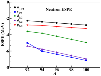
Figure 2: Neutron effective single-particle energies of Mo isotopes calculated with $H_{\rm eff}^{[45]}$.

Therefore, we deem it reasonable the possibility to exclude both $0g_{7/2}$ and $0h_{11/2}$ neutron orbitals, and deal with a smaller model space that should still provide the relevant features of the physics of the nuclei under investigation, namely the parent and grand-daughter nuclei ¹⁰⁰Mo,Ru. However, to calculate the nuclear matrix element for the two-neutrino double-$\beta$ decay $M^{2\nu}$ of ¹⁰⁰Mo we need to retain at least the neutron $0g_{7/2}$ orbital in the model space, otherwise the selection rules of the GT operator would forbid such a decay because of the choice of the proton model subspace.

On these grounds, we derive a new effective Hamiltonian $H_{\rm eff}^{[44]}$, defined within a model space spanned by the $0f_{5/2},1p_{3/2},1p_{1/2},0g_{9/2}$ proton and $0g_{7/2},1d_{5/2},1d_{3/2},2s_{1/2}$ neutron orbitals, by way of a unitary transformation of $H_{\rm eff}^{[45]}$ (see details in Ref. Coraggio et al. (2016)). We label this smaller model space $[44]$ and in Fig. 3 we have reported the energy spectrum of ⁹⁶Mo, that is calculated employing the $H_{\rm eff}^{[45]}$ and $H_{\rm eff}^{[44]}$, and also constraining the action of $H_{\rm eff}^{[45]}$ in the $[44]$ model space.

From the inspection of Fig. 3, it can be noted that $H_{\rm eff}^{[44]}$ is able to provide a better agreement with the energy spectrum obtained through the “mother Hamiltonian” $H^{[45]}$ than the results provided by constraining the diagonalization of the latter Hamiltonian to model space $[44]$. It is also worth pointing out that the values of the $B(E2)$ transition rates, that are calculated with $H_{\rm eff}^{[45]}$ and $H_{\rm eff}^{[44]}$, are very close.

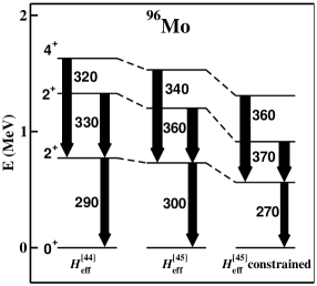
Figure 3: Low-energy spectrum of ⁹⁶Mo, calculated with $H_{\rm eff}^{[45]}$, $H_{\rm eff}^{[44]}$, and constraining $H_{\rm eff}^{[45]}$ in the $[44]$ model space. They are reported also the value of the significant $B(E2)$ transition rates in $e^{2}{\rm fm}^{4}$.

The above results evidence the adequacy of the truncation scheme we have adopted, and the diagonalization of the SM Hamiltonian for ¹⁰⁰Mo and ¹⁰⁰Ru has been performed by way of $H_{\rm eff}^{[44]}$.

The TBMEs of $H_{\rm eff}^{[44]}$, that have been calculated also including three-body correlations to account the number of valence nucleons characterizing ¹⁰⁰Mo, can be found in the Supplemental Material sup .

II.2 Effective shell-model decay operators

We are interested not only in calculating energies, but also the matrix elements of decay operators $\Theta$ which are connected to measurable quantities such as $B(E2)$ strengths, and the nuclear matrix element of the $2\nu\beta\beta$ decay $M^{2\nu}$, as well as the $0\nu\beta\beta$ decay matrix element $M^{0\nu}$.

Since the diagonalization of the $H_{\rm eff}$ does not provide the true wave-functions, but their projections onto the chosen model space $P$, we need to renormalize any decay operator $\Theta$ to take into account the neglected degrees of freedom corresponding to the $Q$-space.

The derivation of SM effective operators within a perturbative approach dates back to the earliest attempts to employ realistic potentials for SM calculations Mavromatis et al. (1966); Mavromatis and Zamick (1967); Federman and Zamick (1969); Ellis and Osnes (1977); Towner and Khanna (1983); Towner (1987), and we follow the procedure that has been introduced by Suzuki and Okamoto in Ref. Suzuki and Okamoto (1995). This allows a calculation of decay operators $\Theta_{\rm eff}$ which is consistent with the one we carry out of $H_{\rm eff}$, and that is based on perturbative expansion of a vertex function $\hat{\Theta}$ box, analogously with the derivation of $H_{\rm eff}$ in terms of the $\hat{Q}$ box (see section II.1). The procedure has been reported in details in Ref. Coraggio and Itaco (2020), and in the following we only report the main building blocks.

The starting point is the perturbative calculation of the two energy-dependent vertex functions

$$\hat{\Theta}(\epsilon)=P\Theta P+P\Theta Q\frac{1}{\epsilon-QHQ}QH_{1}P~{},$$

$$\hat{\Theta}(\epsilon_{1};\epsilon_{2})=PH_{1}Q\frac{1}{\epsilon_{1}-QHQ}Q\Theta Q\frac{1}{\epsilon_{2}-QHQ}QH_{1}P~{},$$

and of their derivatives calculated in $\epsilon=\epsilon_{0}$, $\epsilon_{0}$ being the eigenvalue of the degenerate unperturbed Hamiltonian $H_{0}$:

$$\hat{\Theta}_{m}=\frac{1}{m!}\frac{d^{m}\hat{\Theta}(\epsilon)}{d\epsilon^{m}}\biggl{|}_{\epsilon=\epsilon_{0}}~{},$$

$$\hat{\Theta}_{mn}=\frac{1}{m!n!}\frac{d^{m}}{d\epsilon_{1}^{m}}\frac{d^{n}}{d\epsilon_{2}^{n}}\hat{\Theta}(\epsilon_{1};\epsilon_{2})\biggl{|}_{\epsilon_{1}=\epsilon_{0},\epsilon_{2}=\epsilon_{0}}~{}$$

Then, a series of operators $\chi_{n}$ is calculated:

$$\chi_{0} = (\hat{\Theta}_{0}+h.c.)+\hat{\Theta}_{00}~{}~{},$$ (6)

$$\chi_{1} = (\hat{\Theta}_{1}\hat{Q}+h.c.)+(\hat{\Theta}_{01}\hat{Q}+h.c.)~{}~{},$$

$$\chi_{2} = (\hat{\Theta}_{1}\hat{Q}_{1}\hat{Q}+h.c.)+(\hat{\Theta}_{2}\hat{Q}\hat{Q}+h.c.)+$$

$$(\hat{\Theta}_{02}\hat{Q}\hat{Q}+h.c.)+\hat{Q}\hat{\Theta}_{11}\hat{Q}~{}~{},$$

$$\cdots$$

that allows to write $\Theta_{\rm eff}$ in the following form:

$$\Theta_{\rm eff}=H_{\rm eff}\hat{Q}^{-1}(\chi_{0}+\chi_{1}+\chi_{2}+\cdots)~{}~{}.$$ (8)

In this work we arrest the $\chi_{n}$ series at $n=2$, and the $\hat{\Theta}$ function is expanded up to third order in perturbation theory.

The issue of the convergence of the $\chi_{n}$ series and of the perturbative expansion of the $\hat{\Theta}$ box has been treated in Refs. Coraggio et al. (2018, 2019); Coraggio et al. (2020b), and in Fig. 4 they are reported all the diagrams up to second order appearing in the $\hat{\Theta}(\epsilon_{0})$ expansion for a one-body operator $\Theta$.

Figure 4: One-body second-order diagrams included in the perturbative expansion of $\hat{\Theta}(\epsilon_{0})$. The asterisk indicates the bare operator $\Theta$, the wavy lines the two-body $NN$ interaction, the circle with a cross inside accounts for the ($V\mbox{-}U$)-insertion contribution (see Ref. Coraggio and Itaco (2020)).

In the present work, the decay operators $\Theta$ are the one-body electric-quadrupole transition $E2$ $q_{\scriptscriptstyle{p,n}}r^{2}Y^{2}_{m}(\hat{r})$ – the charge $q_{\scriptscriptstyle{p,n}}$ being $e$ for protons and 0 for neutrons – and GT $\vec{\sigma}\tau^{\pm}$ operators, as well as the two-body transition operator for the $0\nu\beta\beta$decay (see Eqs. (16 – 18) in the following subsection).

II.3 The $2\nu\beta\beta$- and $0\nu\beta\beta$-decay operators

This section is devoted to outline the structure of $2\nu\beta\beta$- and $0\nu\beta\beta$-decay operators.

It is worth pointing out that these two nuclear-decay mechanisms differ in the characteristic value of the momentum transfer, which for $2\nu\beta\beta$ decay is few MeVs, at variance with the order of hundreds of MeVs in $0\nu\beta\beta$ decay. This difference, as we will see in the following, affects the procedure to be followed to calculate $M^{2\nu}$ and $M^{0\nu}$.

As is well known, $2\nu\beta\beta$  decays are the occurrence of two single-$\beta$ decay transitions inside a nucleus, and the expressions of the GT and Fermi components of their nuclear matrix elements $M^{2\nu}$ are the following

$$M_{\rm GT}^{2\nu} = \sum_{n}\frac{\langle 0^{+}_{f}||(\vec{\sigma}\tau^{-})_{\scriptscriptstyle{\mathcal{I}}}||1^{+}_{n}\rangle\langle 1^{+}_{n}||(\vec{\sigma}\tau^{-})_{\scriptscriptstyle{\mathcal{I}}}||0^{+}_{i}\rangle}{E_{n}+E_{0}}~{}~{},$$ (9)

$$M_{\rm F}^{2\nu} = \sum_{n}\frac{\langle 0^{+}_{f}||(\tau^{-})_{\scriptscriptstyle{\mathcal{I}}}||0^{+}_{n}\rangle\langle 0^{+}_{n}||(\tau^{-})_{\scriptscriptstyle{\mathcal{I}}}||0^{+}_{i}\rangle}{E_{n}+E_{0}}~{}~{},$$ (10)

where the subscript $\mathcal{I}$ indicates we are employing the matrix elements of either the bare or the effective one-body GT and F operators.

In these equations, $E_{n}$ is the excitation energy of the $J^{\pi}=0^{+}_{n},1^{+}_{n}$ intermediate state, and $E_{0}=\frac{1}{2}Q_{\beta\beta}(0^{+})+\Delta M$, where $Q_{\beta\beta}(0^{+})$ and $\Delta M$ are the $Q$ value of the transition and the mass difference of the parent and daughter nuclear states, respectively. The index $n$ runs over all possible intermediate states induced by the given transition operator. It should be pointed out that the Fermi component plays a marginal role Haxton and Stephenson Jr. (1984); Elliott and Petr (2002) and in most calculations is neglected altogether.

The most efficient way to obtain $M^{2\nu}$, by including a number of intermediate states that is sufficient to provide the needed accuracy for its calculation, is the Lanczos strength-function method Caurier et al. (2005b) which we have adopted for our calculations.

The evaluation of $M^{2\nu}$ could be also carried out employing the so-called closure approximation, commonly adopted to study $0\nu\beta\beta$-decay NMEs Haxton and Stephenson Jr. (1984). On these grounds, within such an approximation the energies of the intermediate states, $E_{n}$, appearing in Eqs. (9,10), may be replaced by an average value $E_{n}+E_{0}\rightarrow\langle E\rangle$, that allows to avoid to explicitly calculate the intermediate $J^{\pi}=1^{+}_{n}$ states, but then the two one-body transition operators become a two-body operator.

Actually, the closure approximation is a valuable tool to evaluate $M^{0\nu}$, since in the $0\nu\beta\beta$ decay the neutrino’s momentum is about one order of magnitude larger than the average excitation energy of the intermediate states. This allows to neglect, within this process, the intermediate-state-dependent energies from the energy denominator appearing in the neutrino potential, as we will see in a while. On the contrary, the closure approximation is unsatisfactory when used to calculate $M^{2\nu}$, because, as mentioned before, the momentum transfer in $2\nu\beta\beta$ process is much smaller.

Once the theoretical value on $M^{2\nu}$ has been calculated, it can be then compared with the experimental counterpart, which is extracted from the observed half life $T^{2\nu}_{1/2}$

$$\left[T^{2\nu}_{1/2}\right]^{-1}=G^{2\nu}\left|M_{\rm GT}^{2\nu}\right|^{2}~{}~{},$$ (11)

$G^{2\nu}$ being the $2\nu\beta\beta$-decay phase-space (or kinematic) factor Kotila and Iachello (2012, 2013).

We now turn our attention to the bare $0\nu\beta\beta$ operator, for the light-neutrino-exchange channel Engel and Menéndez (2017).

The formal expression of $M_{\alpha}^{0\nu}$ – where $\alpha$ stands for Fermi ($F$), Gamow-Teller (GT), or tensor ($T$) decay channels – is written in terms of the one-body transition-density matrix elements between the daughter and parent nuclei (grand-daughter and daughter nuclei) $\langle k|a^{\dagger}_{p^{\prime}}a_{n^{\prime}}|i\rangle$ ($\langle f|a^{\dagger}_{p}a_{n}|k\rangle$). The subscripts $p$ and $n$ denote proton and neutron states, and $i,k,f$ refer to the parent, daughter, and grand-daughter nuclei, respectively.

The nuclear matrix element $M_{\alpha}^{0\nu}$ is formulated as Sen’kov and Horoi (2013); Šimkovic et al. (2008):

$$M_{\alpha}^{0\nu}= \sum_{k{\cal J}}\sum_{j_{p}j_{p^{\prime}}j_{n}j_{n^{\prime}}}(-1)^{j_{n}+j_{n^{\prime}}+\cal{J}}\hat{\cal{J}}\left\{\begin{array}[]{ccc}j_{p}&j_{n}&J_{\kappa}\\ j_{n^{\prime}}&j_{p^{\prime}}&{\cal J}\end{array}\right\}$$ (14)

$$\left<j_{p}j_{p^{\prime}};{\cal J}\mid\mid\Theta_{\alpha}^{k}\mid\mid j_{n}j_{n^{\prime}};{\cal J}\right>$$

$$\langle k||[a^{\dagger}_{p}\otimes\tilde{a}_{n}]_{J_{k}}||i\rangle\langle k||[a^{\dagger}_{n^{\prime}}\otimes\tilde{a}_{p^{\prime}}]_{J_{k}}||f\rangle^{\ast}=$$

$$\sum_{k}\sum_{j_{p}j_{p^{\prime}}j_{n}j_{n^{\prime}}}\langle f|a^{\dagger}_{p}a_{n}|k\rangle\langle k|a^{\dagger}_{p^{\prime}}a_{n^{\prime}}|i\rangle\times$$

$$\left<j_{p}j_{p^{\prime}}\mid\Theta_{\alpha}^{k}\mid j_{n}j_{n^{\prime}}\right>~{},$$ (15)

where the tilde denotes a time-conjugated state, $\tilde{a}_{jm}=(-1)^{j+m}a_{j-m}$, and the $\Theta_{\alpha}^{k}$ are two-body operators.

The expression of the operators $\Theta_{\alpha}^{k}$ is Engel and Menéndez (2017):

$$\Theta^{k}_{\rm GT} = [\tau^{-}_{1}\tau^{-}_{2}(\vec{\sigma}_{1}\cdot\vec{\sigma}_{2})H_{\rm GT}^{k}(r)]_{\scriptscriptstyle{\mathcal{I}}}\,,$$ (16)

$$\Theta^{k}_{\rm F} = [\tau^{-}_{1}\tau^{-}_{2}H_{\rm F}^{k}(r)]_{\scriptscriptstyle{\mathcal{I}}}\,,$$ (17)

$$\Theta^{k}_{\rm T} = [\tau^{-}_{1}\tau^{-}_{2}\left(3\left(\vec{\sigma}_{1}\cdot\hat{r}\right)\left(\vec{\sigma}_{1}\cdot\hat{r}\right)-\right.$$

$$\left.\vec{\sigma}_{1}\cdot\vec{\sigma}_{2}\right)H_{\rm T}^{k}(r)]_{\scriptscriptstyle{\mathcal{I}}}~{},$$ (18)

where $H_{\alpha}$ are the neutrino potentials and are defined as:

$$H_{\alpha}^{k}(r)=\frac{2R}{\pi}\int_{0}^{\infty}\frac{j_{n_{\alpha}}(qr)h_{\alpha}(q^{2})qdq}{q+E_{k}-(E_{i}+E_{f})/2}~{},$$ (19)

and, again, the subscript ${\mathcal{I}}$ labels the application of either the bare or the effective two-body decay operators.

In Eq. (19), $R=1.2A^{1/3}$ fm, $j_{n_{\alpha}}(qr)$ is the spherical Bessel function, $n_{\alpha}=0$ for Fermi and Gamow-Teller components, while $n_{\alpha}=2$ for the tensor component. In the following, we also present the explicit expressions of neutrino form functions, $h_{\alpha}(q)$, for light-neutrino exchange Engel and Menéndez (2017) :

$$h_{\rm F}({q}^{2}) = g^{2}_{V}({q}^{2})\,,$$

$$h_{\rm GT}({q}^{2}) = \frac{g^{2}_{A}({q}^{2})}{g^{2}_{A}}\left[1-\frac{2}{3}\frac{{q}^{2}}{{q}^{2}+m^{2}_{\pi}}+\frac{1}{3}(\frac{{q}^{2}}{{q}^{2}+m^{2}_{\pi}})^{2}\right]$$

$$+\frac{2}{3}\frac{g^{2}_{M}({q}^{2})}{g^{2}_{A}}\frac{{q}^{2}}{4m^{2}_{p}},$$

$$h_{\rm T}({q}^{2}) = \frac{g^{2}_{A}({q}^{2})}{g^{2}_{A}}\left[\frac{2}{3}\frac{{q}^{2}}{{q}^{2}+m^{2}_{\pi}}-\frac{1}{3}(\frac{{q}^{2}}{{q}^{2}+m^{2}_{\pi}})^{2}\right]$$ (20)

$$+\frac{1}{3}\frac{g^{2}_{M}({q}^{2})}{g^{2}_{A}}\frac{{q}^{2}}{4m^{2}_{p}}\,,$$

In the present work, we use the dipole approximation for the vector, $g_{V}({q}^{2})$, axial-vector, $g_{A}({q}^{2})$, and weak-magnetism, $g_{M}({q}^{2})$, form factors:

$$g_{V}({q}^{2}) = \frac{g_{V}}{(1+{q}^{2}/{\Lambda^{2}_{V}})^{2}},$$

$$g_{M}({q}^{2}) = (\mu_{p}-\mu_{n})g_{V}({q}^{2}),$$

$$g_{A}({q}^{2}) = \frac{g_{A}}{(1+{q}^{2}/{\Lambda^{2}_{A}})^{2}},$$ (21)

where $g_{V}=1$, $g_{A}\equiv g_{A}^{free}=1.2723$, $(\mu_{p}-\mu_{n})=4.7$, and the cutoff parameters $\Lambda_{V}=850$ MeV and $\Lambda_{A}=1086$ MeV.

Then, the total nuclear matrix element $M^{0\nu}$ is written as

$$M^{0\nu}=M_{\rm GT}^{0\nu}-\frac{g_{V}^{2}}{g_{A}^{2}}M_{\rm F}^{0\nu}+M_{\rm T}^{0\nu}~{}~{}.$$ (22)

The expression in Eq. (15) cannot be easily calculated within the nuclear shell model because of the computational complexity of calculating a large number of intermediate states (the Lanczos strength-function method Caurier et al. (2005b) can be applied only for the single-$\beta$-decay process). Therefore, most SM calculations resort to the closure approximation, which is based on the observation that the relative momentum $q$ of the neutrino, appearing in the propagator of Eq. (19), is of the order of 100-200 MeV Engel and Menéndez (2017), and the excitation energies of the nuclei involved in the transition are of the order of 10 MeV Sen’kov and Horoi (2013). On these grounds, the energies of the intermediate states appearing in Eq. (19), may be replaced by an average value $E_{k}-(E_{i}+E_{f})/2\rightarrow\langle E\rangle$, that leads to a simpler form of both Eqs. (15) and (19). Consequently, $M_{\alpha}^{0\nu}$ can be re-written in terms of the two-body transition-density matrix elements $\langle f|a^{\dagger}_{p}a_{n}a^{\dagger}_{p^{\prime}}a_{n^{\prime}}|i\rangle$ as

$$M_{\alpha}^{0\nu} = \sum_{j_{n}j_{n^{\prime}}j_{p}j_{p^{\prime}}}\langle f|a^{\dagger}_{p}a_{n}a^{\dagger}_{p^{\prime}}a_{n^{\prime}}|i\rangle$$

$$\times\left<j_{p}j_{p^{\prime}}\mid\tau^{-}_{1}\tau^{-}_{2}\Theta_{\alpha}\mid j_{n}j_{n^{\prime}}\right>~{},$$ (23)

and the neutrino potentials become

$$H_{\alpha}(r)=\frac{2R}{\pi}\int_{0}^{\infty}\frac{j_{n_{\alpha}}(qr)h_{\alpha}(q^{2})qdq}{q+\left<E\right>}~{}.$$ (24)

As in most SM calculations, we adopt the closure approximation to define the $\Theta$ operators given in Eqs. (16)–(18), and take the average energy $\left<E\right>=11.2$ MeV from the evaluation of Ref. Tomoda (1991). As regards the soundness of the closure approximation to evaluate $M^{0\nu}$, we should point out that in Ref. Sen’kov and Horoi (2013) the authors have performed SM calculations of ⁴⁸Ca $0\nu\beta\beta$ decay both within and beyond the closure approximation, and found that in the second case the results are $\sim 10\%$ larger.

As mentioned in section II.1, one needs to consider short-range correlations when computing the radial matrix elements of the neutrino potentials $\left<\psi_{nl}(r)|H_{\alpha}|\psi_{n^{\prime}l^{\prime}}(r)\right>$.

SRC account for the physics that is missing in all models that expand nuclear wave functions in terms of a truncated non-correlated SP basis Bethe (1971); Kortelainen et al. (2007). This is related to the highly repulsive nature of the short-range two-nucleon interaction, and in order to carry out our SM calculation, that is based on effective operators derived from a realistic potential, we perform a consistent regularization both of the two-nucleon potential, $V^{NN}$, and the $0\nu\beta\beta$-decay operator Coraggio et al. (2020c).

As a matter of fact, the $V_{{\rm low}\mbox{-}k}$ procedure Bogner et al. (2002) renormalizes the repulsive high-momentum components of the $V^{NN}$ potential through a unitary transformation $\Omega$. The latter is an operator which decouples the full momentum space of the two-nucleon Hamiltonian, $H^{NN}$, into two subspaces; the first one is associated with the relative-momentum configurations below a cutoff $\Lambda$ and is specified by a projector operator $P$, the second one is defined in terms of its complement $Q=\mathbf{1}-P$ Coraggio et al. (2020c). As unitary transformation, $\Omega$ preserves the physics of the original potential for the two-nucleon system, namely, the calculated values of all $NN$ observables are the same as those reproduced by solving the Schrödinger equation for two nucleons interacting via $V^{NN}$.

In order to benefit of this procedure, we calculate the two-body $0\nu\beta\beta$  operator, $\Theta$, in the momentum space. Then, $\Theta$ is renormalized using $\Omega$, to provide consistency with the $V^{NN}$ potential, whose high-momentum (short range) components are dumped by the introduction of the cutoff $\Lambda$. The new decay operator is defined as $\Theta_{{\rm low}\mbox{-}k}\equiv P\Omega\Theta\Omega^{-1}P$ for relative momenta $k<\Lambda$, and is set to zero for $k>\Lambda$, and its matrix elements are employed as vertices in the perturbative expansion of the $\hat{\Theta}$ box.

The magnitude of the overall effect of this renormalization procedure is comparable to using the SRC modeled by the Unitary Correlation Operator Method Menéndez et al. (2009), that is a lighter softening of $M^{0\nu}$ with respect to the one provided by Jastrow type SRC Coraggio et al. (2020c).

III Results

In this section we present the results of our SM calculations. First, we compare theoretical and experimental low-energies spectroscopic properties of the parent and granddaughter nuclei ¹⁰⁰Mo and ¹⁰⁰Ru, respectively. We show also the results of the GT^- strength distribution and the calculated NMEs of the $2\nu\beta\beta$ decay for ¹⁰⁰Mo and compare them with the available data.

Then, we calculate the nuclear matrix element of the $0\nu\beta\beta$ decay and study the convergence behavior of the effective SM operator we have derived consistently with $H_{\rm eff}$. We also discuss the effects of three-valence-nucleon diagrams which correct the Pauli-principle violation introduced in systems with more than two valence nucleons Towner (1987).

As already mentioned, all the calculations are performed employing theoretical SP energies and TBMEs obtained from the effective Hamiltonian $H_{\rm eff}^{[44]}$, whose model space is defined by $0f_{5/2},1p_{3/2},1p_{1/2},0g_{9/2}$ proton and $0g_{7/2},1d_{5/2},1d_{3/2},2s_{1/2}$ neutron orbitals, that can be found in the Supplemental Material sup .

III.1 Spectroscopy of ¹⁰⁰Mo and ¹⁰⁰Ru

In Fig. 5, we compare the calculated low-energy spectra of ¹⁰⁰Mo and ¹⁰⁰Ru, as well as their experimental counterparts.

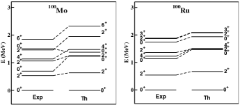
Figure 5: Experimental and calculated spectra of ¹⁰⁰Mo and ¹⁰⁰Ru up to 2 MeV excitation energy.

As can be seen, our $H_{\rm eff}$ provides a reasonable reproduction of ¹⁰⁰Mo low-lying states, despite the large number of valence nucleons involved in the diagonalization of the SM Hamiltonian. The larger discrepancy between observed and theoretical spectra occurs for the yrare $J^{\pi}=0^{+}$ state, which exhibits experimentally a pronounced collective behavior. This is also testified by the $B(E2)$ strength between the $J^{\pi}=0^{+}_{2}$ and $J^{\pi}=2^{+}_{1}$ levels, that is reported in Table 3. In fact, from the inspection of Table 3, we see that there is a general agreement between theoretical and experimental values, but our calculation fails to reproduce the large $B(E2;0^{+}_{2}\rightarrow 2^{+}_{1})$.

Once more, it is worth stressing that to calculate the $B(E2)$ strengths the effective proton/neutron charges have been derived from theory (see Sec. II.2), without any empirical adjustment, and whose values can be found in Table 2.

Table 2: Proton and neutron effective charges of the electric quadrupole operator $E2$.

$n_{a}l_{a}j_{a}~{}n_{b}l_{b}j_{b}$	$\langle a||e_{p}||b\rangle$	$n_{a}l_{a}j_{a}~{}n_{b}l_{b}j_{b}$	$\langle a||e_{n}||b\rangle$
$0f_{5/2}~{}0f_{5/2}$	1.62	$0g_{7/2}~{}0g_{7/2}$	1.00
$0f_{5/2}~{}1p_{3/2}$	1.45	$0g_{7/2}~{}1d_{5/2}$	0.73
$0f_{5/2}~{}1p_{1/2}$	1.47	$0g_{7/2}~{}1d_{3/2}$	0.70
$1p_{3/2}~{}0f_{5/2}$	1.28	$1d_{5/2}~{}0g_{7/2}$	0.68
$1p_{3/2}~{}1p_{3/2}$	1.20	$1d_{5/2}~{}1d_{5/2}$	0.47
$1p_{3/2}~{}1p_{1/2}$	1.21	$1d_{5/2}~{}1d_{3/2}$	0.48
$1p_{1/2}~{}0f_{5/2}$	1.31	$1d_{5/2}~{}2s_{1/2}$	0.43
$0g_{1/2}~{}1p_{3/2}$	1.22	$1d_{3/2}~{}0g_{7/2}$	0.66
$0g_{9/2}~{}0g_{9/2}$	1.70	$1d_{3/2}~{}1d_{5/2}$	0.48
		$1d_{3/2}~{}1d_{3/2}$	0.55
		$1d_{3/2}~{}2s_{1/2}$	0.50
		$2s_{1/2}~{}1d_{5/2}$	0.43
		$2s_{1/2}~{}1d_{3/2}$	0.50
		$0h_{11/2}~{}0h_{11/2}$	0.79

As regards the low-energy spectrum of ¹⁰⁰Ru, our calculation provides a satisfactory reproduction of the experiment, and this is also testified by the comparison of the theoretical $B(E2)$ strengths with the available data, as reported in Table 4.

Table 3: Experimental and calculated $B(E2)$ strengths (in $e^{2}{\rm fm}^{4}$) for ¹⁰⁰Mo, data are taken from Ref. ens . We report those for the observed states in Fig. 5.

$J_{i}\rightarrow J_{f}$	$B(E2)_{\rm Expt}$	$B(E2)_{\rm Calc}$
$2^{+}_{1}\rightarrow 0^{+}_{1}$	$1000\pm 100$	820
$0^{+}_{2}\rightarrow 2^{+}_{1}$	$2500\pm 100$	55
$2^{+}_{2}\rightarrow 0^{+}_{1}$	$17\pm 1$	30
$2^{+}_{2}\rightarrow 2^{+}_{1}$	$1400\pm 140$	800
$2^{+}_{2}\rightarrow 0^{+}_{2}$	$150\pm 20$	540
$4^{+}_{1}\rightarrow 2^{+}_{1}$	$1900\pm 100$	1200
$2^{+}_{3}\rightarrow 2^{+}_{1}$	$8\pm 2$	15
$2^{+}_{3}\rightarrow 0^{+}_{2}$	$400\pm 100$	340
$6^{+}_{1}\rightarrow 4^{+}_{1}$	$2500\pm 400$	1240

Table 4: Experimental and calculated $B(E2)$ strengths (in $e^{2}{\rm fm}^{4}$) for ¹⁰⁰Ru, data are taken from Ref. ens . We report those for the observed states in Fig. 5.

$J_{i}\rightarrow J_{f}$	$B(E2)_{\rm Expt}$	$B(E2)_{\rm Calc}$
$2^{+}_{1}\rightarrow 0^{+}_{1}$	$980\pm 10$	640
$0^{+}_{2}\rightarrow 2^{+}_{1}$	$1000\pm 140$	300
$4^{+}_{1}\rightarrow 2^{+}_{1}$	$1400\pm 100$	980
$2^{+}_{2}\rightarrow 2^{+}_{1}$	$850\pm 170$	570
$2^{+}_{2}\rightarrow 0^{+}_{1}$	$55\pm 10$	50
$2^{+}_{3}\rightarrow 4^{+}_{1}$	$500\pm 140$	90
$2^{+}_{3}\rightarrow 0^{+}_{2}$	$1000\pm 250$	360

We now proceed to examine the results of the calculation of quantities that are directly related to the double-$\beta$ decay of ¹⁰⁰Mo. It is worth pointing out that, because of the proton and neutron model spaces, the effective GT⁺ operator consists of one matrix element that corresponds to the $\pi 0g_{9/2}\rightarrow\nu 0g_{7/2}$ decay, whose calculated quenching factor is $q=0.454$. Similarly, the only matrix element of the effective GT^- operator $\nu 0g_{9/2}\rightarrow\pi 0g_{7/2}$ provides a quenching factor $q=0.503$.

The reason of a non-hermitian effective GT-decay operator is threefold; the proton and neutron model spaces we have chosen are different, the proton-neutron symmetry is broken because the Coulomb interaction is included in the perturbative expansion, the procedure that has been followed to derive the effective operators is non-hermitian Suzuki and Okamoto (1995).

In Table 5 we report the observed and calculated values of the $M^{2\nu}$s for the $2\nu\beta\beta$ decay of ¹⁰⁰Mo from the $J^{\pi}=0^{+}_{1}$ ground state (g.s.) to the ¹⁰⁰Ru $J^{\pi}=0^{+}_{1},0^{+}_{2}$ states. For both decays the value of $M^{2\nu}$  obtained with the bare operator overestimates the experimental one by a factor $3\div 4$, but employing the matrix elements of the effective GT⁺ and GT^- operators we reach a result that is in a good agreement with the observed $M^{2\nu}$s.

Table 5: Experimental Barabash (2020) and calculated $M^{2\nu}$s (in MeV^-1) for ¹⁰⁰Mo $2\nu\beta\beta$ decay. The theoretical values are obtained employing both the bare (I) and effective (II) $2\nu\beta\beta$ operators.

100Mo$\rightarrow^{100}$Ru decay branches	Experiment	I	II
$J^{\pi}=0^{+}_{1}\rightarrow J^{\pi}=0^{+}_{1}$	$0.224\pm 0.002$	0.896	0.205
$J^{\pi}=0^{+}_{1}\rightarrow J^{\pi}=0^{+}_{2}$	$0.182\pm 0.006$	0.479	0.109

In Fig. 6, the calculated $\sum{\rm B(GT)}$ for ¹⁰⁰Mo are shown as a function of the ¹⁰⁰Tc excitation energy, and compared with the data reported with a red line Thies et al. (2012). The results obtained with the bare operator are drawn with a blue line, while those obtained employing the effective GT operator are plotted a black line.

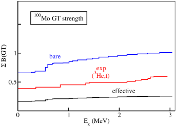
Figure 6: Running sums of the ¹⁰⁰Mo $\sum{\rm B(GT)}$ strengths as a function of the excitation energy $E_{x}$ up to 3 MeV.

It can be seen that the distribution obtained using the bare operator overestimates the observed one, but the quenching induced by the effective operator provides an underestimation of the values extracted from the experiment.

Here, it should be reminded that the ”experimental” GT strengths obtained from charge-exchange reactions are not directly observed data. The GT strength can be extracted from the GT component of the cross section at zero degree, following the standard approach in the distorted-wave Born approximation (DWBA).

$$\frac{d\sigma^{GT}(0^{\circ})}{d\Omega}=\left(\frac{\mu}{\pi\hbar^{2}}\right)^{2}\frac{k_{f}}{k_{i}}N^{\sigma\tau}_{D}|J_{\sigma\tau}|^{2}B({\rm GT})~{}~{},$$

where $N^{\sigma\tau}_{D}$ is the distortion factor, $|J_{\sigma\tau}|$ is the volume integral of the effective $NN$ interaction, $k_{i}$ and $k_{f}$ are the initial and final momenta, respectively, and $\mu$ is the reduced mass (see formula and description in Refs. Puppe et al. (2012); Frekers et al. (2013)). Then, the values of experimental GT strengths are somehow model-dependent.

III.2 Neutrinoless double-$\beta$ decay of ¹⁰⁰Mo

As introduced in Section II, our calculation of $M^{0\nu}$ accounts for the light-neutrino exchange mechanism, the total nuclear matrix element being expressed as in Eq. (22) and calculated accordingly to Eqs. (16,17,18,23,24), namely within the closure approximation.

The perturbative expansion of the $0\nu\beta\beta$ effective operator $\Theta_{\rm eff}$  has been carried out including in the $\hat{\Theta}$ box  diagrams up to the third order (see Section II), and a number of intermediate states which corresponds to oscillator quanta up to $N_{\rm max}=14$, since the results are substantially convergent from $N_{\rm max}=12$ on (see Ref. Coraggio et al. (2020b)).

As regards the expansion of $\Theta_{\rm eff}$ as a function of the $\chi_{n}$ operators, we stop at $n=2$ since $\chi_{3}$ depends on the first, second, and third derivatives of $\hat{\Theta}_{0}$ and $\hat{\Theta}_{00}$, as well as on the first and second derivatives of the $\hat{Q}$ box (see Eq. (II.2)), so $\chi_{3}$ contribution may be estimated at least one order of magnitude smaller than the $\chi_{2}$ one. Moreover, in Ref Coraggio et al. (2020b) we have shown that the contributions from $\chi_{1}$ are relevant, while those from $\chi_{2}$ are almost negligible.

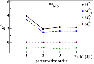
Figure 7: $M^{0\nu}$ for the decay of the ¹⁰⁰Mo $J^{\pi}=0^{+}_{1}$ state to the ¹⁰⁰Ru $J^{\pi}=0^{+}_{1}$ one, as a function of the perturbative order. The green triangles correspond to $M^{0\nu}_{\rm F}$, the blue squares to $M^{0\nu}_{\rm GT}$, the magenta diamonds to $M^{0\nu}_{\rm T}$, and the black dots to the full $M^{0\nu}$.

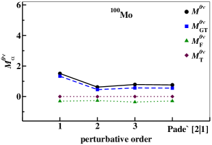
Figure 8: Same as in Fig. 7, but for the decay of the ¹⁰⁰Mo $J^{\pi}=0^{+}_{1}$ state to the ¹⁰⁰Ru $J^{\pi}=0^{+}_{2}$ one.

First, we focus on the results of the order-by-order convergence behavior by reporting in Figs. 7,8 the calculated values of $M^{0\nu}$, $M^{0\nu}_{\rm GT}$, $M^{0\nu}_{\rm F}$, and $M^{0\nu}_{\rm T}$ for both the decay of the ¹⁰⁰Mo $J^{\pi}=0^{+}_{1}$ state to the ¹⁰⁰Ru $J^{\pi}=0^{+}_{1},0^{+}_{2}$ ones, respectively, from first- up to third-order in perturbation theory. As an indicator of the quality of the perturbative behavior Baker and Gammel (1970), we also report the value of their Padé approximant $[2|1]$. We also point out that the same scale has been adopted in both figures.

As in other decays we have studied in our previous work Coraggio et al. (2020b), the perturbative behavior is driven by the Gamow-Teller component, since the Fermi matrix element $M^{0\nu}_{\rm F}$ is weakly affected by the renormalization procedure, and $M^{0\nu}_{\rm T}$ is almost negligible. We observe a perturbative pattern of the calculated $M^{0\nu}$ of ¹⁰⁰Mo that is better than the ones we have found for ⁴⁸Ge, ⁷⁶Ge, ⁸²Se, ¹³⁰Te, and ¹³⁶Xe $0\nu\beta\beta$ decays, which have been calculated within the same approach Coraggio et al. (2020b). In fact, here the difference between second- and third-order results is about $13\%$ and $21\%$ for the decay of the ¹⁰⁰Mo $J^{\pi}=0^{+}_{1}$ state to the ¹⁰⁰Ru $J^{\pi}=0^{+}_{1}$ and $J^{\pi}=0^{+}_{2}$ ones, respectively.

Table 6: Calculated values of $M^{0\nu}$ for the decay of ¹⁰⁰Mo g.s. state to the yrast and yrare $J^{\pi}=0^{+}$ states of ¹⁰⁰Ru.

$0^{+}_{1}\rightarrow 0^{+}_{1}$
	$M^{0\nu}_{\rm GT}$	$M^{0\nu}_{\rm F}$	$M^{0\nu}_{\rm T}$	$M^{0\nu}$
Present work (I)	3.418	-0.878	0.002	3.962
Present work (II)	1.634	-0.970	0.007	2.240
IBM-2 Barea et al. (2015)	3.73	-0.48	0.19	4.22
EDF Vaquero et al. (2013)	5.361	-1.986		6.588
BMF-CDFT Yao et al. (2015)				10.91
pnQRPA Šimkovic et al. (2013)	4.950	-2.367	-0.571	5.850
pnQRPA Hyvärinen and Suhonen (2015)	3.13	-1.03	-0.26	3.90
$0^{+}_{1}\rightarrow 0^{+}_{2}$
	$M^{0\nu}_{\rm GT}$	$M^{0\nu}_{\rm F}$	$M^{0\nu}_{\rm T}$	$M^{0\nu}$
Present work (I)	1.344	-0.308	0.001	1.535
Present work (II)	0.564	-0.361	0.001	0.788
IBM-2 Barea et al. (2015)	0.99	-0.13	0.05	1.12

In Table 6 the values of $M^{0\nu}$, which we have calculated by using both the bare operator – namely without condidering neither SRC nor renormalizations due to the truncation of the model space – and $\Theta_{\rm eff}$, have been reported, as well as their Gamow-Teller, Fermi, and tensor components. Our results are also compared with those obtained employing other nuclear models, such as the interacting boson model with isospin restoration (IBM-2) Barea et al. (2015), the energy density functional method including deformation and pairing fluctuations (EDF) Vaquero et al. (2013), the beyond-mean-field covariant density functional theory (BMF-CDFT) Yao et al. (2015), and quasiparticle random-phase approximation with isospin symmetry restoration (pnQRPA) Šimkovic et al. (2013); Hyvärinen and Suhonen (2015).

The SM results obtained with the bare $0\nu\beta\beta$  operator (I) can be better compared with other nuclear models, since in the latter no effective operator has been considered, and we see that our $M^{0\nu}$s are close to those in Refs. Barea et al. (2015); Hyvärinen and Suhonen (2015), where the IBM-2 and pnQRPA models have been employed, respectively. The other calculations provide $M^{0\nu}$s  that are much larger than our result, and it is worth pointing out that different choices of the parameters for pnQRPA calculations may lead to a remarkable difference of the calculated $M^{0\nu}$s Šimkovic et al. (2013); Hyvärinen and Suhonen (2015).

The action of the effective operator $\Theta_{\rm eff}$  quenches the value of the two $M^{0\nu}$s  by a factor about one half, whose effect is smaller than accounting for the quenching factor of the axial coupling constant $g_{A}$ that comes out from the calculated effective GT^± operator, which is about $q=0.5$.

These considerations are related to the question if one should relate the derivation of the effective one-body GT operator Coraggio et al. (2019) with the renormalization of the two-body GT component of the $0\nu\beta\beta$ operator. As a matter of fact, this issue has a considerable impact on the detectability of $0\nu\beta\beta$ process Suhonen (2017a, b).

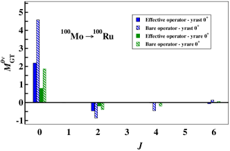
Figure 9: Contributions from pairs of decaying neutrons with given $J^{\pi}$ to $M^{0\nu}_{\rm GT}$ for ¹⁰⁰Mo $0\nu\beta\beta$ decay. The bars filled in blue corresponds to the results obtained with $\Theta_{\rm eff}$, those in dashed blue to the ones calculated with bare operator

To complete our discussion about the $M^{0\nu}$s, we show in Figs. 9, 10 the results of the decomposition of $M^{0\nu}_{\rm GT}$ and $M^{0\nu}_{\rm F}$, respectively, in terms of the contributions from the decaying pair of neutrons coupled to a given angular momentum and parity $J^{\pi}$, both for the decay to the ¹⁰⁰Ru ground (blue columns) and yrare $J^{\pi}=0^{+}$ (green columns) states.

We report the contributions obtained by employing both the effective $0\nu\beta\beta$-decay  operator $\Theta_{\rm eff}$ (colour filled columns) and the bare one (dashed filled columns).

The results of the decomposition of $M^{0\nu}_{\rm F}$ confirm the irrelevance of the renormalization procedure, and exhibit the dominance of the $J^{\pi}=0^{+}$ component.

As regards $M^{0\nu}_{\rm GT}$, as it should be expected, each $J^{\pi}$ contribution calculated employing $\Theta_{\rm eff}$  is much smaller than the one obtained with the bare $0\nu\beta\beta$-decay operator. The main contributions, both employing effective and bare operators, correspond to the $J^{\pi}=0^{+},2^{+}$ components, being opposite in sign, and a non-negligible role is played by the $J^{\pi}=4^{+}$ component too.

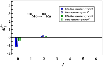
Figure 10: Same as in Fig. 9, but for $M^{0\nu}_{\rm F}$.

IV Summary and outlook

This work is the first attempt to calculate double-$\beta$ decay of ¹⁰⁰Mo into ¹⁰⁰Ru by way of the nuclear shell model.

Our study has consisted first in verifying the ability of the tools we have chosen, namely the model space and the shell-model effective Hamiltonian and decay operators, to reproduce the experimental spectroscopic properties of ¹⁰⁰Mo,Ru – excitation spectra and $B(E2)$ strengths that are related to the collective behavior of these systems – as well as the nuclear matrix elements $M^{2\nu}$ of the $2\nu\beta\beta$-decay and the GT strengths obtained from charge-exchange reactions. Then, after having tested and shown the degree of reliability of our wave functions, we have calculated the nuclear matrix elements $M^{0\nu}$s  of the $0\nu\beta\beta$-decay of the ¹⁰⁰Mo ground state to the yrast and yrare $J^{\pi}=0^{+}$ states of ¹⁰⁰Ru.

An important feature of our work is that shell-model effective Hamiltonians and decay operators have been derived by way of many-body perturbation theory, starting from a high-precision realistic potential CD-Bonn Machleidt (2001). Such an approach has been previously applied to study the ⁴⁸Ca$\rightarrow^{48}$Ti, ⁷⁶Ge$\rightarrow^{76}$Se, ⁸²Se$\rightarrow^{82}$Kr, ¹³⁰Te$\rightarrow^{130}$Xe, and ¹³⁶Xe$\rightarrow^{136}$Ba decays Coraggio et al. (2017, 2019); Coraggio et al. (2020b).

The comparison of our results with the available data seems to indicate that the realistic shell model can quantitatively describe most of the spectroscopy (low-lying excitation spectra, electromagnetic transition strengths) of ¹⁰⁰Mo,Ru and also their $\beta$-decay properties (nuclear matrix elements of $2\nu\beta\beta$ decay, GT strengths from charge-exchange reactions) without resorting to empirical adjustments of $H_{\rm eff}$, effective charges, or quenching the axial coupling constant. This should provide support to our approach for the prediction of the $M^{0\nu}$s for the $0\nu\beta\beta$ decay of ¹⁰⁰Mo, within the light-neutrino-exchange channel, that is a conjugation of the action of shell-model wave functions, emerging from the diagonalization of $H_{\rm eff}$, and effective decay operators, which are constructed consistently with $H_{\rm eff}$.

We have also compared our results for the $0\nu\beta\beta$ decay of ¹⁰⁰Mo with those obtained employing other nuclear methods, leading to some relevant observations. To this end, we have considered the results we obtain employing both the bare $0\nu\beta\beta$  operator – namely without any sort of normalization – and the effective operator derived theoretically. The $M^{0\nu}$s  we calculate with the bare operator are important for a fair comparison with other nuclear models, since the latter do not employ any effective operator which accounts for the truncation of the Hilbert space.

First, it can be noticed that our results with the bare operator are consistent with recent calculations performed with IBM-2 Barea et al. (2015) and pnQRPA Hyvärinen and Suhonen (2015), whereas the results obtained within EDF Vaquero et al. (2013) and BMF-CDFT Yao et al. (2015) approaches, as well as pnQRPA calculations performed by Šimkovic et al. Šimkovic et al. (2013), provide larger values of $M^{0\nu}$s.

Second, as in our previous study Coraggio et al. (2020b), the effect of the renormalization of the $0\nu\beta\beta$-decay operator, with respect to the truncation of the full Hilbert space to the shell-model one, is smaller than the one obtained for the $2\nu\beta\beta$-decay one.

These results may be a valuable asset for the community that is involved with the experimental detection of the ¹⁰⁰Mo $0\nu\beta\beta$-decay, since this is the first time a microscopic calculation has been performed of the $M^{0\nu}$s  of the ¹⁰⁰Mo ground-state decay to the two lowest-in-energy $J^{\pi}=0^{+}$ states of ¹⁰⁰Ru.

Our future program to upgrade the study of nuclei with mass $A\approx 100$ which are candidates to $0\nu\beta\beta$-decay is twofold.

On one side, we plan to start from nuclear forces that own a firm link with QCD, namely we will construct effective shell-model Hamiltonians and decay-operators from two- and three-body potentials derived within the framework of chiral perturbation theory Fukui et al. (2018); Ma et al. (2019); Coraggio et al. (2020d).

This step will allow us:

1. to evaluate the dependence of the predictions for $M^{0\nu}$s  on the nuclear potential that is employed in a nuclear structure calculation;

2. to benchmark our results with those obtained with ab initio calculations Yao et al. (2020); Novario et al. (2021); Belley et al. (2021);

3. to consider the contribution of the two-body meson-exchange corrections to the electroweak currents, originated from sub-nucleonic degrees of freedom, that can be consistently tackled employing nuclear chiral potentials.

On the other side, we are currently exploring the possibility to employ larger model spaces, that would account better for the low-energy collective behavior of nuclei with mass $A\approx 100$. This would provide major informations about the connection between the calculated values of the $M^{0\nu}$s and the dimension of the model space, and how theoretical effective decay-operators can compensate and reduce this dependence.

These goals are computationally challenging, but we are confident that our current efforts may lead in a close future to a first set of preliminary results.

References

- Fukuda et al. (1998) Y. Fukuda, T. Hayakawa, E. Ichihara, K. Inoue, K. Ishihara, H. Ishino, Y. Itow, T. Kajita, J. Kameda, S. Kasuga, et al. (Super-Kamiokande Collaboration), Phys. Rev. Lett. 81, 1562 (1998).
- Ahmad et al. (2001) Q. R. Ahmad, R. C. Allen, T. C. Andersen, J. D. Anglin, G. Bühler, J. C. Barton, E. W. Beier, M. Bercovitch, J. Bigu, S. Biller, et al. (SNO Collaboration), Phys. Rev. Lett. 87, 071301 (2001).
- Falcone and Tramontano (2001) D. Falcone and F. Tramontano, Phys. Rev. D 64, 077302 (2001).
- Mohapatra and Smirnov (2006) R. Mohapatra and A. Smirnov, Annu. Rev. Nucl. Part. Sci. 56, 569 (2006).
- Dell’Oro et al. (2016) S. Dell’Oro, S. Marcocci, M. Viel, and F. Vissani, Adv. High Energy Phys. 2016, 2162659 (2016).
- Kotila and Iachello (2012) J. Kotila and F. Iachello, Phys. Rev. C 85, 034316 (2012).
- Kotila and Iachello (2013) J. Kotila and F. Iachello, Phys. Rev. C 87, 024313 (2013).
- Avignone et al. (2008) F. T. Avignone, S. R. Elliott, and J. Engel, Rev. Mod. Phys. 80, 481 (2008).
- Tanabashi et al. (2018) M. Tanabashi, K. Hagiwara, K. Hikasa, K. Nakamura, Y. Sumino, F. Takahashi, J. Tanaka, K. Agashe, G. Aielli, C. Amsler, et al. (Particle Data Group), Phys. Rev. D 98, 030001 (2018).
- Pastore et al. (2018) S. Pastore, J. Carlson, V. Cirigliano, W. Dekens, E. Mereghetti, and R. B. Wiringa, Phys. Rev. C 97, 014606 (2018).
- Cirigliano et al. (2018) V. Cirigliano, W. Dekens, J. de Vries, M. L. Graesser, E. Mereghetti, S. Pastore, and U. van Kolck, Phys. Rev. Lett. 120, 202001 (2018).
- Cirigliano et al. (2019) V. Cirigliano, W. Dekens, J. de Vries, M. L. Graesser, E. Mereghetti, S. Pastore, M. Piarulli, U. van Kolck, and R. B. Wiringa, Phys. Rev. C 100, 055504 (2019).
- Yao et al. (2020) J. M. Yao, B. Bally, J. Engel, R. Wirth, T. R. Rodríguez, and H. Hergert, Phys. Rev. Lett. 124, 232501 (2020).
- Novario et al. (2021) S. Novario, P. Gysbers, J. Engel, G. Hagen, G. R. Jansen, T. D. Morris, P. Navrátil, T. Papenbrock, and S. Quaglioni, Phys. Rev. Lett. 126, 182502 (2021).
- Belley et al. (2021) A. Belley, C. G. Payne, S. R. Stroberg, T. Miyagi, and J. D. Holt, Phys. Rev. Lett. 126, 042502 (2021).
- Barea et al. (2013) J. Barea, J. Kotila, and F. Iachello, Phys. Rev. C 87, 014315 (2013).
- Terasaki (2015) J. Terasaki, Phys. Rev. C 91, 034318 (2015).
- Fang et al. (2018) D.-L. Fang, A. Faessler, and F. Šimkovic, Phys. Rev. C 97, 045503 (2018).
- Rodríguez and Martínez-Pinedo (2010) T. R. Rodríguez and G. Martínez-Pinedo, Phys. Rev. Lett. 105, 252503 (2010).
- Rodríguez and Gabriel (2013) T. R. Rodríguez and M.-P. Gabriel, Phys. Lett. B 719, 174 (2013).
- Yao et al. (2015) J. M. Yao, L. S. Song, K. Hagino, P. Ring, and J. Meng, Phys. Rev. C 91, 024316 (2015).
- Song et al. (2017) L. S. Song, J. M. Yao, P. Ring, and J. Meng, Phys. Rev. C 95, 024305 (2017).
- Jiao et al. (2017) C. F. Jiao, J. Engel, and J. D. Holt, Phys. Rev. C 96, 054310 (2017).
- Jiao et al. (2018) C. F. Jiao, M. Horoi, and A. Neacsu, Phys. Rev. C 98, 064324 (2018).
- Sen’kov and Horoi (2013) R. A. Sen’kov and M. Horoi, Phys. Rev. C 88, 064312 (2013).
- Holt and Engel (2013) J. D. Holt and J. Engel, Phys. Rev. C 87, 064315 (2013).
- Sen’kov et al. (2014) R. A. Sen’kov, M. Horoi, and B. A. Brown, Phys. Rev. C 89, 054304 (2014).
- Neacsu and Horoi (2015) A. Neacsu and M. Horoi, Phys. Rev. C 91, 024309 (2015).
- Menéndez (2017) J. Menéndez, J. Phys. G 45, 014003 (2017).
- Coraggio et al. (2020a) L. Coraggio, N. Itaco, G. De Gregorio, A. Gargano, R. Mancino, and S. Pastore, Universe 6, 233 (2020a).
- Wang et al. (2017) M. Wang, G. Audi, F. G. Kondev, W. J. Huang, S. Naimi, and X. Xing, Chin. Phys. C 41, 030003 (2017).
- Alenkov et al. (2019) V. Alenkov, H. W. Bae, J. Beyer, R. S. Boiko, K. Boonin, O. Buzanov, N. Chanthima, M. K. Cheoun, D. M. Chernyak, J. S. Choe, et al., Eur. Phys. J. C 79, 791 (2019).
- Bhang et al. (2012) H. Bhang, R. S. Boiko, D. M. Chernyak, J. H. Choi, S. Choi, F. A. Danevich, K. V. Efendiev, C. Enss, A. Fleischmann, A. M. Gangapshev, et al., Journal of Physics: Conference Series 375, 042023 (2012).
- Arnold et al. (2007) R. Arnold, C. Augier, J. Baker, A. Barabash, M. Bongrand, G. Broudin, V. Brudanin, A. Caffrey, V. Egorov, A. Etienvre, et al., Nucl. Phys. A 781, 209 (2007).
- Armengaud et al. (2020) E. Armengaud, C. Augier, A. S. Barabash, F. Bellini, G. Benato, A. Benoît, M. Beretta, L. Bergé, J. Billard, Y. A. Borovlev, et al. (CUPID-Mo Collaboration), Eur. Phys. J. C 80, 674 (2020).
- Armengaud et al. (2021) E. Armengaud, C. Augier, A. S. Barabash, F. Bellini, G. Benato, A. Benoît, M. Beretta, L. Bergé, J. Billard, Y. A. Borovlev, et al. (CUPID-Mo Collaboration), Phys. Rev. Lett. 126, 181802 (2021).
- The CUPID Interest Group (2019) The CUPID Interest Group, arXiv:1907.09376[physics] (2019).
- Cheifetz et al. (1970) E. Cheifetz, R. C. Jared, S. G. Thompson, and J. B. Wilhelmy, Phys. Rev. Lett. 25, 38 (1970).
- von Brentano et al. (2004) P. von Brentano, V. Werner, R. F. Casten, C. Scholl, E. A. McCutchan, R. Krücken, and J. Jolie, Phys. Rev. Lett. 93, 152502 (2004).
- Cejnar and Jolie (2004) P. Cejnar and J. Jolie, Phys. Rev. C 69, 011301 (2004).
- Zhang et al. (2015) C. L. Zhang, G. H. Bhat, W. Nazarewicz, J. A. Sheikh, and Y. Shi, Phys. Rev. C 92, 034307 (2015).
- Xiang et al. (2016) J. Xiang, J. M. Yao, Y. Fu, Z. H. Wang, Z. P. Li, and W. H. Long, Phys. Rev. C 93, 054324 (2016).
- Abusara et al. (2017) H. Abusara, S. Ahmad, and S. Othman, Phys. Rev. C 95, 054302 (2017).
- Johnstone and Towner (1998) I. P. Johnstone and I. S. Towner, Eur. Phys. J. A 3, 237 (1998).
- Özen and Dean (2006) C. Özen and D. J. Dean, Phys. Rev. C 73, 014302 (2006).
- Vaquero et al. (2013) N. L. Vaquero, T. R. Rodríguez, and J. L. Egido, Phys. Rev. Lett. 111, 142501 (2013).
- Barea et al. (2015) J. Barea, J. Kotila, and F. Iachello, Phys. Rev. C 91, 034304 (2015).
- Tomoda (1991) T. Tomoda, Rep. Prog. Phys. 54, 53 (1991).
- Pantis et al. (1996) G. Pantis, F. Šimkovic, J. D. Vergados, and A. Faessler, Phys. Rev. C 53, 695 (1996).
- Chaturvedi et al. (2003) K. Chaturvedi, B. M. Dixit, P. K. Rath, and P. K. Raina, Phys. Rev. C 67, 064317 (2003).
- Šimkovic et al. (2013) F. Šimkovic, V. Rodin, A. Faessler, and P. Vogel, Phys. Rev. C 87, 045501 (2013).
- Hyvärinen and Suhonen (2015) J. Hyvärinen and J. Suhonen, Phys. Rev. C 91, 024613 (2015).
- Coraggio et al. (2009) L. Coraggio, A. Covello, A. Gargano, N. Itaco, and T. T. S. Kuo, Prog. Part. Nucl. Phys. 62, 135 (2009).
- Machleidt (2001) R. Machleidt, Phys. Rev. C 63, 024001 (2001).
- Bogner et al. (2002) S. Bogner, T. T. S. Kuo, L. Coraggio, A. Covello, and N. Itaco, Phys. Rev. C 65, 051301(R) (2002).
- Kuo et al. (1995) T. T. S. Kuo, F. Krmpotić, K. Suzuki, and R. Okamoto, Nucl. Phys. A 582, 205 (1995).
- Hjorth-Jensen et al. (1995) M. Hjorth-Jensen, T. T. S. Kuo, and E. Osnes, Phys. Rep. 261, 125 (1995).
- Suzuki and Okamoto (1995) K. Suzuki and R. Okamoto, Prog. Theor. Phys. 93, 905 (1995).
- Coraggio et al. (2012) L. Coraggio, A. Covello, A. Gargano, N. Itaco, and T. T. S. Kuo, Ann. Phys. (NY) 327, 2125 (2012).
- Ellis and Osnes (1977) P. J. Ellis and E. Osnes, Rev. Mod. Phys. 49, 777 (1977).
- Coraggio and Itaco (2020) L. Coraggio and N. Itaco, Frontiers in Physics 8, 345 (2020).
- Coraggio et al. (2017) L. Coraggio, L. De Angelis, T. Fukui, A. Gargano, and N. Itaco, Phys. Rev. C 95, 064324 (2017).
- Coraggio et al. (2019) L. Coraggio, L. De Angelis, T. Fukui, A. Gargano, N. Itaco, and F. Nowacki, Phys. Rev. C 100, 014316 (2019).
- Coraggio et al. (2020b) L. Coraggio, A. Gargano, N. Itaco, R. Mancino, and F. Nowacki, Phys. Rev. C 101, 044315 (2020b).
- Sieja et al. (2009) K. Sieja, F. Nowacki, K. Langanke, and G. Martínez-Pinedo, Phys. Rev. C 79, 064310 (2009).
- Coraggio et al. (2016) L. Coraggio, A. Gargano, and N. Itaco, Phys. Rev. C 93, 064328 (2016).
- Coraggio et al. (2015) L. Coraggio, A. Covello, A. Gargano, N. Itaco, and T. T. S. Kuo, Phys. Rev. C 91, 041301 (2015).
- Coraggio et al. (2020c) L. Coraggio, N. Itaco, and R. Mancino, J. Phys. Conf. Ser. 1643, 012124 (2020c).
- Kuo and Osnes (1990) T. T. S. Kuo and E. Osnes, Lecture Notes in Physics, vol. 364 (Springer-Verlag, Berlin, 1990).
- Krenciglowa and Kuo (1974) E. M. Krenciglowa and T. T. S. Kuo, Nucl. Phys. A 235, 171 (1974).
- Suzuki and Lee (1980) K. Suzuki and S. Y. Lee, Prog. Theor. Phys. 64, 2091 (1980).
- Suzuki et al. (2011) K. Suzuki, R. Okamoto, H. Kumagai, and S. Fujii, Phys. Rev. C 83, 024304 (2011).
- Caurier et al. (2005a) E. Caurier, G. Martínez-Pinedo, F. Nowacki, A. Poves, and A. P. Zuker, Rev. Mod. Phys. 77, 427 (2005a).
- Coraggio et al. (2020d) L. Coraggio, G. De Gregorio, A. Gargano, N. Itaco, T. Fukui, Y. Z. Ma, and F. R. Xu, Phys. Rev. C 102, 054326 (2020d).
- (75) See Supplemental Material at [URL will be inserted by publisher] for the list of two-body matrix elements of the shell-model Hamiltonian , derived for 14 and 8 valence protons and neutrons, respectively, namely for 100Mo.
- Mavromatis et al. (1966) H. A. Mavromatis, L. Zamick, and G. E. Brown, Nucl. Phys. A 80, 545 (1966).
- Mavromatis and Zamick (1967) H. A. Mavromatis and L. Zamick, Nucl. Phys. A 104, 17 (1967).
- Federman and Zamick (1969) P. Federman and L. Zamick, Phys. Rev. 177, 1534 (1969).
- Towner and Khanna (1983) I. S. Towner and K. F. C. Khanna, Nucl. Phys. A 399, 334 (1983).
- Towner (1987) I. S. Towner, Phys. Rep. 155, 263 (1987).
- Coraggio et al. (2018) L. Coraggio, L. De Angelis, T. Fukui, A. Gargano, and N. Itaco, J. Phys. Conf. Ser. 1056, 012012 (2018).
- Haxton and Stephenson Jr. (1984) W. C. Haxton and G. J. Stephenson Jr., Prog. Part. Nucl. Phys. 12, 409 (1984).
- Elliott and Petr (2002) S. R. Elliott and V. Petr, Annu. Rev. Nucl. Part. Sci. 52, 115 (2002).
- Caurier et al. (2005b) E. Caurier, G. Martínez-Pinedo, F. Nowacki, A. Poves, and A. P. Zuker, Rev. Mod. Phys. 77, 427 (2005b).
- Engel and Menéndez (2017) J. Engel and J. Menéndez, Rep. Prog. Phys. 80, 046301 (2017).
- Šimkovic et al. (2008) F. Šimkovic, A. Faessler, V. Rodin, P. Vogel, and J. Engel, Phys. Rev. C 77, 045503 (2008).
- Bethe (1971) H. A. Bethe, Annu. Rev. Nucl. Sci. 21, 93 (1971).
- Kortelainen et al. (2007) M. Kortelainen, O. Civitarese, J. Suhonen, and J. Toivanen, Phys. Lett. B 647, 128 (2007).
- Menéndez et al. (2009) J. Menéndez, A. Poves, E. Caurier, and F. Nowacki, Nucl. Phys. A 818, 139 (2009).
- (90) Data extracted using the NNDC On-line Data Service from the ENSDF database, file revised as of March 13, 2021., URL https://www.nndc.bnl.gov/ensdf.
- Barabash (2020) A. Barabash, Universe 6, 159 (2020).
- Thies et al. (2012) J. H. Thies, T. Adachi, M. Dozono, H. Ejiri, D. Frekers, H. Fujita, Y. Fujita, M. Fujiwara, E.-W. Grewe, K. Hatanaka, et al., Phys. Rev. C 86, 044309 (2012).
- Puppe et al. (2012) P. Puppe, A. Lennarz, T. Adachi, H. Akimune, H. Ejiri, D. Frekers, H. Fujita, Y. Fujita, M. Fujiwara, E. Ganioğlu, et al., Phys. Rev. C 86, 044603 (2012).
- Frekers et al. (2013) D. Frekers, P. Puppe, J. H. Thies, and H. Ejiri, Nucl. Phys. A 916, 219 (2013).
- Baker and Gammel (1970) G. A. Baker and J. L. Gammel, The Padé Approximant in Theoretical Physics, vol. 71 of Mathematics in Science and Engineering (Academic Press, New York, 1970).
- Suhonen (2017a) J. Suhonen, Phys. Rev. C 96, 055501 (2017a).
- Suhonen (2017b) J. T. Suhonen, Frontiers in Physics 5, 55 (2017b).
- Fukui et al. (2018) T. Fukui, L. De Angelis, Y. Z. Ma, L. Coraggio, A. Gargano, N. Itaco, and F. R. Xu, Phys. Rev. C 98, 044305 (2018).
- Ma et al. (2019) Y. Z. Ma, L. Coraggio, L. De Angelis, T. Fukui, A. Gargano, N. Itaco, and F. R. Xu, Phys. Rev. C 100, 034324 (2019).