Weakly Supervised Correspondence Learning

Abstract

Correspondence learning is a fundamental problem in robotics, which aims to learn a mapping between state, action pairs of agents of different dynamics or embodiments. However, current correspondence learning methods either leverage strictly paired data—which are often difficult to collect—or learn in an unsupervised fashion from unpaired data using regularization techniques such as cycle-consistency—which suffer from severe misalignment issues. We propose a weakly supervised correspondence learning approach that trades off between strong supervision over strictly paired data and unsupervised learning with a regularizer over unpaired data. Our idea is to leverage two types of weak supervision: i) temporal ordering of states and actions to reduce the compounding error, and ii) paired abstractions, instead of paired data, to alleviate the misalignment problem and learn a more accurate correspondence. The two types of weak supervision are easy to access in real-world applications, which simultaneously reduces the high cost of annotating strictly paired data and improves the quality of the learned correspondence. We show the videos of the experiments on our website.

I Introduction

Humans are born with the ability to develop new skills by mimicking the behavior of others who may have different embodiments [1]. For example, prior cognitive science work suggest that 1- or 2-year-old children can infer the intentions of adults and re-enact their behavior with their own body even with a large difference in body structures [2, 3]. We refer to the ability to infer the mapping between the state, action pairs of agents with different dynamics or embodiment as correspondence learning. Correspondence learning is essential in robotics where we have limited data and would like to learn from demonstrations from other agents.

To learn the correspondence between agents, several prior works leverage paired trajectories to learn invariant representations across agents [4, 5, 6, 7], where the representation only preserves the information that is relevant to the downstream tasks. However, collecting and annotating paired trajectories require experts with substantial domain knowledge and is usually expensive to access at large scale.

Due to the difficulties of collecting paired data, several works propose learning the correspondence between environments as a translation map between the agents using unpaired trajectories [8, 9]. The key insight of these works is adopting a regularization term over the translation model, where cycle-consistency is the most commonly used regularization [10, 11, 12, 13]. However, with no supervision, the quality of the learned correspondence model is usually not as good as models learned with strong supervision over paired data [14, 15].

In this paper, we propose Weakly Supervised Correspondence Learning (WeaSCL) to find a trade-off between strong supervision of strictly paired data and regularization over unpaired data. Our key insight is to leverage weak supervision that is useful for learning correspondence and also is easy to access in real-world applications. We propose two types of weak supervision: i) temporal ordering in states and actions, and ii) paired abstractions over data.

The temporal ordering, which originates from the nature of sequential decisions, indicates the temporal dependency of the consecutive states and actions. Leveraging temporal dependency as a measure of weak supervision enables us to avoid compounding errors of translation maps that can be accumulated over long horizons.

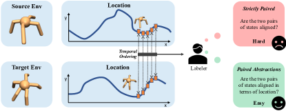
Figure 1: An example of the paired abstractions. Given two trajectories of a four- and five-legged ant robots, it is difficult to decide whether two full states that include joint angles of each agent are aligned, while it is easy to align simpler abstractions such as spatial location.

We define paired abstractions by a similarity metric over some abstraction of states or state-action pairs of the agents. For example, the location of a mobile robot, the pose of an end-effector, or the confidence of a behavior can potentially be suitable abstractions over data. When learning correspondence between two agents, one can consider a pair of these abstractions as opposed to paired data. The paired abstractions are easier to obtain and annotate than strictly paired data, as annotators would have an easier time comparing similarity over simpler abstractions. For example, in Fig. 1, it would be difficult to align the full states including the joint angles of the trajectories of a four- and five-legged Ant. On the other hand, it is much easier and more informative to decide if an abstraction of the state, e.g., the location of the Ant agents on the 2D plane are aligned. In our work, we collect such paired abstractions and learn a similarity function over this data. We then incorporate this similarity function in the loss function imposing a constraint on the translation maps. In summary, the contributions of this paper are:

• We propose a weakly supervised correspondence learning approach to address the shortcomings of using strictly paired data or using unpaired data with regularization.

• Our approach utilizes weak supervision (temporal ordering over states and paired abstractions over data) to learn correspondence. This weak supervision enforces multi-step dynamics cycle-consistency over a sequence of states and actions and also imposes a similarity function learned from paired abstractions as a constraint in correspondence learning.

• Our empirical results on cross-morphology, cross-physics, and cross-modality correspondence learning tasks in Mujoco, simulated robot, and real robot environments show that WeaSCL achieves much higher performance compared to prior methods.

II Related Works

Learning Invariant Representations. To learn the correspondence across agents, one line of works learn an invariant representation of states and actions, which remove any dependencies on unrelated information for the downstream task and only preserve task-specific information [16, 17, 18, 4, 5, 19]. Domain randomization methods learn generalizable domain invariant representations by augmenting the current domain, but they require the variation of the applied domains to be covered by the augmentation [17, 20, 18, 16, 21, 22, 23, 24, 25]. This assumption is restrictive and requires the full domain information to design effective augmentations. Other works remove this assumption and learn invariant representations from paired trajectories [4, 5, 26, 19]. However, supervision over paired trajectories require domain expertise, which is expensive or even impossible to collect [27]. Instead of such strong supervision, our approach uses weak supervision to learn the correspondence, which is easier to annotate.

Learning Translation Maps. Due to the challenges of collecting paired data, approaches that use unpaired data are proposed to learn a translation map between the agents’ trajectories [28, 29, 30, 31, 32, 10, 33]. Most of the works on learning translation maps are proposed in the visual domains. Cycle-consistency was proposed to address image translation across different domains and it achieves promising results [8]. Many follow up works improve the stability of the training and the quality of the translated images [34, 8, 35, 11, 9, 36, 12, 10, 37]. Recent works propose utilizing weakly aligned images to learn the translation [30]. Going beyond visual observations, Ammar et al. use unsupervised manifold alignment to find the correspondence between states across domains from demonstrations but they rely on hand-designed features, which restricts generalization [29]. Kim et al. propose to imitate demonstrations by building correspondence between the agents but assume the MDPs are ‘alignable’ with respect to a definition of MDP reduction [32].

Recently, dynamic cycle-consistency (DCC) is proposed to learn a translation map over the states and actions across domains [13]. DCC is not restricted to the visual domains and is proven to be applicable to different physics, modalities, and morphologies. Though achieving the state-of-the-art performance with unpaired trajectories, DCC still does not perform as well as methods with strong supervision. Our approach is closely related to DCC, but also imposes weak supervision over DCC to learn a more accurate translation map without the need for highly costly annotations.

Learning with Insufficient Annotations. For particular tasks, the exact annotations of the task are difficult to obtain, which results in different learning frameworks to deal with limited annotations. Semi-supervised learning aims to learn from little labeled data and large-scale unlabeled data. For correspondence learning, the small slice of data can be annotated by keyframes extraction and segmentation [38, 39]. However, such accurate annotations are sometimes impossible to provide even with expert knowledge. Thus, weakly supervised learning is proposed to leverage weak supervision that provides imprecise or inexact but easy-to-access labels [40]. Weakly supervised learning has been used in robotics and control tasks such as goal-orientated reinforcement learning [41] and goal-directed navigation [42], which substantially reduces the exploration space. However, in correspondence learning, prior works often only consider strong supervision, i.e., using strictly paired trajectories or they only rely on regularization along with unpaired data. In this work, we focus on leveraging weakly supervised learning in correspondence learning.

III Correspondence Learning:
Problem and Background

In this section, we introduce the problem of correspondence learning and provide some background on dynamic cycle-consistency first introduced by [13].

Correspondence Learning. We focus on learning correspondence between two agents. However, we note that one can extend this to multiple agents by building correspondence between pairs of agents. We model each agent as a deterministic Markov Decision Process (MDP): $\mathcal{M}^{1}=(\mathcal{S}^{1},\mathcal{A}^{1},\mathcal{T}^{1},\mathcal{R}^{1},p^{1}_{0},\gamma)$ and $\mathcal{M}^{2}=(\mathcal{S}^{2},\mathcal{A}^{2},\mathcal{T}^{2},\mathcal{R}^{2},p^{2}_{0},\gamma)$. Similar to [13], we define a correspondence from $\mathcal{M}^{1}$ to $\mathcal{M}^{2}$ as follows: Let $\Phi:\mathcal{S}^{1}\rightarrow\mathcal{S}^{2}$ be a state map, and $H^{1}:\mathcal{S}^{1}\times\mathcal{A}^{1}\rightarrow\mathcal{A}^{2}$ and $H^{2}:\mathcal{S}^{2}\times\mathcal{A}^{2}\rightarrow\mathcal{A}^{1}$ be two action maps, where the state map and the action maps satisfy the following requirements: $\forall s^{1}\in\mathcal{S}^{1}$, if $s^{2}=\Phi(s^{1})$, then $\forall a^{1}\in\mathcal{A}^{1},\Phi(\mathcal{T}^{1}(s^{1},a^{1}))=\mathcal{T}^{2}(s^{2},H^{1}(s^{1},a^{1}))$ and $\forall a^{2}\in\mathcal{A}^{2},\Phi(\mathcal{T}^{1}(s^{1},H^{2}(s^{2},a^{2})))=\mathcal{T}^{2}(s^{2},a^{2})$. Intuitively, the requirements mean that the successor states of the two aligned states should be aligned if taking aligned actions.

Using this correspondence definition, we are now ready to introduce our problem statement. We assume access to three pieces of information: a set of trajectories (sequence of state, action pairs) $\Xi^{1}=\{\xi^{1}\}$ for $M^{1}$, a set of trajectories $\Xi^{2}=\{\xi^{2}\}$ for $M^{2}$, and one or multiple sets of paired abstractions over the states or over the state-action pairs. Specifically, we have $K^{s}$ sets of paired abstractions over states: $Y_{1}^{s},Y_{2}^{s},\dots,Y_{K^{s}}^{s}$ and $K^{a}$ sets of paired abstractions over state-action pairs. Each $Y_{k}^{s}$ is a set of pairs of states and similarity labels over abstractions of states: $Y_{k}^{s}=\{(s^{1},s^{2},v^{s})\}$, where $v^{s}\in[0,1]$ reflects the similarity of one choice of abstraction, e.g., the pose of an end-effector, over the state $s^{1}$ and $s^{2}$. Note that the data tuples $(s^{1},s^{2},v^{s})$ are given by annotators, where the annotators decide which abstraction to take and how to annotate similarity. Our algorithm does not have access to the choice of abstraction and similarity but aims to learn a similarity function $\Phi^{\text{weak}}_{k}:\mathcal{S}^{1}\times\mathcal{S}^{2}\rightarrow[0,1]$ mapping the raw pairs of states to a similarity value based on the given data tuples. Similarly each $Y_{k}^{a}=\{((s^{1},a^{1}),(s^{2},a^{2}),v^{a})\}$ and $v^{a}\in[0,1]$ reflects the similarity of a choice of abstraction over $(s^{1},a^{1})$ and $(s^{2},a^{2})$, and we aim to learn a similarity function $H^{\text{weak}}_{k}:\mathcal{S}^{1}\times\mathcal{A}^{1}\times\mathcal{S}^{2}\times\mathcal{A}^{2}\rightarrow[0,1]$ mapping the raw pairs of state-action pairs to the similarity value. Our goal in correspondence learning is to learn the state map $\Phi$ and the action maps $H^{1}$ and $H^{2}$ with $\Xi^{1}$, $\Xi^{2}$, and the similarity functions learned from the paired abstraction data $Y_{1}^{s},\dots,Y_{K^{s}}^{s}$ and $Y_{1}^{a},\dots,Y_{K^{a}}^{a}$.

We emphasize that the paired abstractions only consider a loose alignment between the states and actions of the two MDPs. Such loose pairing of the states—pairing of abstractions over states—simply can be assessed by visual observations, and collecting such data along with annotations is much easier, and can serve as a cheap supervision.

Background on Dynamics Cycle-Consistency. Dynamic Cycle-Consistency (DCC) [13] first uses adversarial learning to ensure that the states mapped by $\Phi$ fall into the domain of $\mathcal{M}^{2}$. Specifically, one can learn $\Phi$ with a discriminator $D^{s}$ by the following adversarial objective:

$$\min\limits_{\Phi}\max\limits_{D^{s}}\mathcal{L}^{s}_{\text{adv}}(\Phi,D^{s})=$$ (1)

$$\mathbb{E}_{s^{2}\sim\Xi^{2}}[D^{s}(s^{2})]+\mathbb{E}_{s^{1}\sim\Xi^{1}}[1-D^{s}(\Phi(s^{1}))].$$

In addition, DCC ensures that the actions mapped by $H^{1}$ and $H^{2}$ also match the actions in the domain of $\mathcal{M}^{2}$ and $\mathcal{M}^{1}$ using discriminators $D^{a^{1}}$ and $D^{a^{2}}$ respectively:

$$\min\limits_{H^{1},H^{2}}\max\limits_{D^{a^{1}},D^{a^{2}}}\mathcal{L}^{a}_{\text{adv}}(H^{1},H^{2},D^{a^{1}},D^{a^{2}})=$$ (2)

$$\quad\mathbb{E}_{a^{2}\sim\Xi^{2}}[D^{a^{2}}(a^{2})]+\mathbb{E}_{(s^{1},a^{1})\sim\Xi^{1}}[1-D^{a^{2}}(H^{1}(s_{1},a^{1}))]$$

$$+\mathbb{E}_{a^{1}\sim\Xi^{1}}[D^{a^{1}}(a^{1})]+\mathbb{E}_{(s^{2},a^{2})\sim\Xi^{2}}[1-D^{a^{1}}(H^{2}(s_{2},a^{2}))].$$

Finally, one can add a domain cycle-consistency objective on the state-action maps $H^{1}$ and $H^{2}$:

$$\min\limits_{H^{1},H^{2}}\mathcal{L}_{\text{dom\_con}}(H^{1},H^{2})=$$ (3)

$$\quad\mathbb{E}_{(s^{1},a^{1})\in\Xi^{1}}\left[\lVert H^{2}\left(\Phi(s^{1}),H^{1}(s^{1},a^{1})\right)-a^{1}\rVert\right]$$

$$+\mathbb{E}_{(s^{2},a^{2})\in\Xi^{2}}\left[\lVert H^{1}\left(\Phi(s^{2}),H^{2}(s^{2},a^{2})\right)-a^{2}\rVert\right].$$

This equation ensures that the two action maps are consistent with each other and the translated action should be able to be translated back.

The adversarial training as proposed so far suffers from the mode collapse problem [43], where multiple states for one agent can potentially be mapped to one state in the other. In addition, the domain cycle-consistency cannot solve the problem when the two maps $H^{1}$ and $H^{2}$ make consistent mistakes. For example, we can map $(s^{1},a^{1})$ to an incorrect action, e.g., $\bar{a}^{2}$, by $H^{1}$ and map it back to $a^{1}$ by $H^{2}$. Here, both maps make mistakes but the domain consistency is still preserved. To address this issue, DCC introduces the dynamics cycle-consistency objective:

$$\min\limits_{\Phi,H^{1}}\mathcal{L}_{\text{dyn\_con}}(\Phi,H^{1})=$$

$$\quad\mathbb{E}_{(s^{1}_{t},a^{1}_{t},s^{1}_{t+1})\sim\Xi^{1}}\left[\left\lVert\Phi(s^{1}_{t+1})-\mathcal{T}^{2}\left(\Phi(s^{1}_{t}),H^{1}(s^{1}_{t},a^{1}_{t})\right)\right\rVert\right].$$

Here, the transition function $\mathcal{T}^{2}$ for $\mathcal{M}^{2}$ is not always known and can be non-differentiable. So one can empirically learn a transition function $\hat{\mathcal{T}}^{2}$ using the following objective:

$$\small\min\limits_{\hat{\mathcal{T}}^{2}}\mathcal{L}_{\text{forward}}(\hat{\mathcal{T}}^{2})=\mathbb{E}_{(s^{2}_{t},a^{2}_{t},s^{2}_{t+1})\sim\Xi^{2}}\left[\left\lVert s^{2}_{t+1}-\hat{\mathcal{T}}^{2}(s^{2}_{t},a^{2}_{t})\right\rVert\right].$$

Combining all the losses introduced so far, the final optimization objective is:

$$\mathcal{L}_{\text{DCC}}= \lambda_{0}\mathcal{L}_{\text{dyn\_con}}(\Phi,H^{1})+\lambda_{1}\mathcal{L}_{\text{dom\_con}}(H^{1},H^{2})$$

$$+\lambda_{2}\mathcal{L}^{a}_{\text{adv}}(H^{1},H^{2},D^{a^{1}},D^{a^{2}})+\lambda_{3}\mathcal{L}^{s}_{\text{adv}}(\Phi,D^{s}),$$

where $\lambda_{0}$, $\lambda_{1}$, $\lambda_{2}$ and $\lambda_{3}$ are hyperparameters trading off between the different losses. DCC firstly trains the forward dynamics $\hat{\mathcal{T}}^{2}$ and then trains the translation model with $\mathcal{L}_{\text{DCC}}$.

Limitations of DCC. Here, we discuss two core shortcomings of DCC—compounding error and misalignment—which can lead to errors in the translation model.

The compounding error problem refers to the fact that the single step errors from the state and actions maps can accumulate over a sequence. We empirically demonstrate the existence of compounding errors by selecting a segment of a trajectory with horizon $T$: $\xi^{1}=\{s^{1}_{0},a^{1}_{0},\dots,s^{1}_{T}\}$ in $\Xi^{1}$. We use two methods to derive the translated state at time step $T$: (1) $s^{2}_{T}=\Phi(s^{1}_{T})$; (2) $\hat{s}^{2}_{T}=\mathcal{T}^{2}\left(\cdots\mathcal{T}^{2}\left(\Phi(s^{1}_{0}),H_{1}(s^{1}_{0},a^{1}_{0})\right),\dots,H_{1}(s^{1}_{T},a^{1}_{T})\right)$. The second method continuously uses the translated action to generate the next state to follow the transition process in $\xi^{1}$. We experiment in the Mujoco HalfCheetah environment to build a correspondence between the two-legged and three-legged robots. As shown in Fig. 2(a), the distance of $s^{2}_{T}$ and $\hat{s}^{2}_{T}$ for DCC gets larger over time, which suggests the existence of compounding errors in the action maps. Our hypothesis is that this is due to the fact that dynamics cycle-consistency is only ensured for one time step and leads to a small error in that step but cannot bound the error over a long horizon.

Dynamic Cycle-Consistency still suffers from misalignment issues. For example, assume we are given two trajectories $\xi^{1}_{A}$ and $\xi^{1}_{B}$ for the agent following $\mathcal{M}^{1}$ and two trajectories $\xi^{2}_{A}$ and $\xi^{2}_{B}$ for the agent following $\mathcal{M}^{2}$, where the four trajectories have the same number of time steps. Let’s assume the ground-truth translation should translate $\xi^{1}_{A}$ to $\xi^{2}_{A}$ and $\xi^{1}_{B}$ to $\xi^{2}_{B}$. However, if one only enforces dynamics cycle-consistency, it is possible to learn a map that translates the states and actions at each step from $\xi^{1}_{A}$ to $\xi^{2}_{A}$ and from $\xi^{1}_{B}$ to $\xi^{2}_{B}$, or translates from $\xi^{1}_{A}$ to $\xi^{2}_{B}$ and from $\xi^{1}_{B}$ to $\xi^{2}_{A}$, where both maps have zero errors in terms of dynamics cycle-consistency. So the misalignment issue can occur without strong supervision of paired data. However, strictly paired data is often difficult to collect, and we thus aim for some intermediate supervision such as learning similarities between paired abstractions over states, which are much easier to annotate.

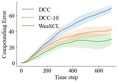
(a) Compounding Error

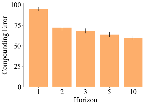
(b) Different Horizon

Figure 2: (a) The translation error at each time step. (b) The compounding error with respect to different final horizons.

IV Weakly Supervised Correspondence Learning

We propose weakly supervised correspondence learning (WeaSCL) to address the above issues with two weak supervision: temporal ordering and paired abstraction data.

Multi-Step Dynamics Cycle-Consistency. As we discussed in Sec. III, even a small error for the state map and the action maps at each step will cause a large deviation in a long horizon because DCC only enforces one-step consistency and the error can accumulate across time steps given no constraint. To address this problem, we use the weak supervision of consecutive states and actions to enforce the dynamics cycle-consistency over multiple steps. The new loss can be formulated as follows:

$$\min\limits_{\Phi,H^{1}}\mathcal{L}_{\text{m\_dyn\_con}}(\Phi,H^{1})=\mathbb{E}_{(s^{1}_{t},a^{1}_{t},s^{1}_{t+1},\cdots,s^{1}_{t+T})\sim\Xi^{1}}\sum\limits_{\tau=1}^{T}$$ (4)

$$\quad\left[\left\lVert\Phi(s^{1}_{t+\tau})-\hat{\mathcal{T}}^{2}\left(\cdots\hat{\mathcal{T}}^{2}\left(\Phi(s^{1}_{t}),\hat{a}^{2}_{t}\right)\cdots\hat{a}^{2}_{t+\tau-1}\right)\right\rVert\right],$$

where $\hat{a}^{2}_{t}=H_{1}(s^{1}_{t},a^{1}_{t})$ is the translated action at time $t$ and $T$ is the final horizon to enforce dynamics cycle-consistency. With this new loss, as shown in Fig. 2(a), with final horizon $10$, the compounding error is substantially reduced.

Now we should consider how long to enforce the dynamics cycle-consistency. We conduct an experiment on the performance of translation with respect to the final horizon in the HalfCheetah environment. We create two agents $\mathcal{M}^{1}$ with three legs and $\mathcal{M}^{2}$ with two legs. We translate the states of $\mathcal{M}^{1}$ to $\mathcal{M}^{2}$ with $\Phi$ and take the optimal action based on the optimal policy of $\mathcal{M}^{2}$. We then translate the action back to $\mathcal{M}^{1}$ with $H^{2}$. In Fig. 2(b), we observe that the performance of translation increases with a longer horizon at first but saturates from horizon $5$ onwards.

Learning Correspondence by Weak Supervision. To address the misalignment issue, we adopt weak supervision from paired abstractions, where a similarity metric is defined on the abstractions (e.g. the location, end-effector pose, or confidence score) The key difference between strictly paired data and paired abstractions is that strictly paired data need to comprehensively assess all the aspects of the two states or state-action pairs, which is difficult to collect. On the other hand, paired abstractions only consider similarities over an abstraction of the state, which are thus easier to annotate.

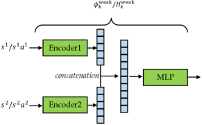
Figure 3: The architecture of the similarity function. The states or state-action pairs from the two agents are first mapped by their individual encoders to a shared hidden space. The hidden features are concatenated and mapped to the similarity value with a multi-layer perceptron.

We first learn a similarity function from each set of paired abstraction data, which is modelled as a neural network with a pair of states or state-action pairs as input and outputs a similarity value in $[0,1]$. The architecture is shown in Fig. 3. We first map the input states from both agents to the same hidden space by their individual encoder and concatenate the two hidden features. Then we use a fully-connected network to map the concatenated feature to the scalar similarity value. The losses for all the similarity functions are

$$\min\limits_{\Phi^{\text{weak}}_{k}}\mathcal{L}^{s}_{k}(\Phi^{\text{weak}}_{k})=\mathbb{E}_{(s^{1},s^{2},v^{s})\sim Y_{k}^{s}}\ell({\Phi^{\text{weak}}_{k}(s^{1},s^{2})},v^{s})$$ (5)

$$\min\limits_{H^{\text{weak}}_{k}}\mathcal{L}^{a}_{k}(H^{\text{weak}}_{k})=$$

$$\quad\quad\quad\mathbb{E}_{((s^{1},a^{1}),(s^{2},a^{2}),v^{s})\sim Y_{k}^{s}}\ell({H^{\text{weak}}_{k}(s^{1},a^{2},s^{2},a^{2})},v^{s}),$$

where $\ell$ takes the binary cross entropy loss to minimize the difference between the predicted and the ground-truth similarity. Then, we impose the learned similarity function as a constraint on the state map and the action maps:

$$\min\limits_{\Phi}\mathcal{L}^{\text{weak}}_{s}(\Phi)=\sum\limits_{k=1}^{K^{s}}\mathbb{E}_{s^{1}\in\Xi^{1}}\left[-\Phi^{\text{weak}}_{k}(s^{1},\Phi(s^{1}))\right]$$ (6)

$$\min\limits_{H^{1}}\mathcal{L}^{\text{weak}}_{a}(H^{1})=$$

$$\quad\sum\limits_{k=1}^{K^{a}}\mathbb{E}_{(s^{1},a^{1})\in\Xi^{1}}\left[-H^{\text{weak}}_{k}(s^{1},a^{1},\Phi(s^{1}),H^{1}(s^{1},a^{1}))\right].$$

We minimize the negative similarity to ensure the states and the translated states are similar as well as the state-action pairs and the translated state-action pairs stay similar. With the above constraint, the misalignment of the learned translation model will be substantially reduced. Also, as shown in Fig. 2(a), paired abstractions can reduce the compounding error by reducing the translation error at each step.

Overall Loss and Algorithm. Integrating all the losses, we derive the final learning objective of our model as follows:

$$\mathcal{L}_{\text{all}}= \lambda_{0}\mathcal{L}_{\text{m\_dyn\_con}}(\Phi,H^{1})+\lambda_{1}\mathcal{L}_{\text{dom\_con}}(H^{1},H^{2})$$ (7)

$$+\lambda_{2}\mathcal{L}^{a}_{\text{adv}}(H^{1},H^{2},D_{a^{1}},D_{a^{2}})+\lambda_{3}\mathcal{L}^{s}_{\text{adv}}(\Phi,D_{s})$$

$$+\lambda_{4}(\mathcal{L}^{\text{weak}}_{s}(\Phi)+\mathcal{L}^{\text{weak}}_{a}(H^{1}))$$

where $\lambda_{4}$ is the trade-off parameter for the weakly supervised loss. Jointly optimizing all the loss functions in Eqn. (7) can cause unstable training  [7]. Thus, we first learn the forward model $\hat{\mathcal{T}}^{2}$ and the similarity functions $\Phi^{\text{weak}}_{1}-\Phi^{\text{weak}}_{K^{s}}$ and $H^{\text{weak}}_{1}-H^{\text{weak}}_{K^{a}}$. After converging, we fix their parameters. Then, we iteratively train the networks related to the state map: $\Phi$ and $D^{s}$, and the networks related to the action maps: $H^{1}$, $H^{2}$, $D^{a^{1}}$ and $D^{a^{2}}$. When we train $\Phi$ and $D^{s}$, we fix the parameters of $H^{1}$, $H^{2}$, $D^{a^{1}}$, and $D^{a^{2}}$, and vice versa. Such an iterative training paradigm avoids the state map and the action maps converging to unstable solutions. When training $\Phi$ and $D^{s}$ or $H^{1},H^{2}$, and $D^{a^{1}},D^{a^{2}}$, we follow the training paradigm of adversarial networks [43].

V Experiments

In our experiments, we aim to demonstrate the efficacy of WeaSCL in different correspondence learning settings including cross-morphology, cross-physics, and cross-modality, and demonstrate that WeaSCL works well with different types of paired abstractions in different environments.

We use WeaSCL-$T$ to refer to our approach, where $T$ corresponds to the final horizon at which we enforce dynamics cycle-consistency. We compare WeaSCL-$T$ with baseline methods: DCC [7] and CC, which removes the dynamics cycle-consistency in DCC, and several variants of WeaSCL: DCC-$T$ and WeaSCL-1, where DCC-$T$ only adopts multi-step dynamics cycle-consistency without using paired abstractions while WeaSCL-1 uses the paired abstractions but only uses single-step dynamics cycle-consistency.

V-A Cross-Morphology

TABLE I: Morphology parameters and dimension of state and action spaces in the HalfCheetah, Swimmer and Ant.

Environment	Agent $\mathcal{M}^{2}$			Agent $\mathcal{M}^{1}$
	Morphology	State	Action	Morphology	State	Action
HalfCheetah	2 legs	18	6	3 legs	24	9
Swimmer	3 links	10	2	4 links	12	3
Ant	4 legs	113	8	5 legs	135	10

Mujoco Environments. We conduct our experiments in Mujoco HalfCheetah, Swimmer, and Ant environments under a cross-morphology setting, where we create different agents by varying the morphology. The morphology and the dimension of state space and action space are shown in Table I. The goal of this task is to learn and evaluate a translation model to leverage the optimal policy for the agent $\mathcal{M}^{1}$ to make decisions in the environment of agent $\mathcal{M}^{2}$. We measure the similarity of states using the x-axis location as the abstraction of the state. Since both state spaces and action spaces are different, we train both the state map $\Phi$ and action maps $H^{1}$ and $H^{2}$. The number of similarity pairs used for all three environments are 1,000 each.

The results are shown in Table II. For both DCC and our methods, using a horizon of $5$ for dynamics cycle-consistency achieves a much better performance than a horizon of $1$, which demonstrates the efficacy of multi-step dynamics cycle-consistency. WeaSCL-5 and WeaSCL-1 outperform DCC-5 and DCC-1 respectively, which demonstrates the efficacy of paired abstractions.

TABLE II: The performance of the translated policy under different morphologies in Mujoco environments.

Method	HalfCheetah	Swimmer	Ant
CC	-104.39$\pm$92.72	30.00$\pm$2.19	297.52$\pm$87.48
DCC-1	658.66$\pm$23.13	53.40$\pm$11.39	447.50$\pm$470.19
DCC-2	1005.52$\pm$44.12	64.92$\pm$5.43	669.94$\pm$72.54
DCC-3	1166.90$\pm$ 50.67	71.70$\pm$3.53	762.43$\pm$1.92
DCC-5	1250.55$\pm$ 51.66	65.19$\pm$ 2.16	928.22$\pm$ 1.96
DCC-10	1249.15$\pm$434.78	52.18$\pm$3.61	942.03$\pm$ 2.61
WeaSCL-1	1284.61$\pm$109.47	69.59$\pm$13.88	969.28$\pm$1.03
WeaSCL-5	1455.08$\pm$63.59	86.14$\pm$2.46	971.08$\pm$2.10
Oracle	4380.75$\pm$97.30	126.19$\pm$2.42	991.56$\pm$1.98

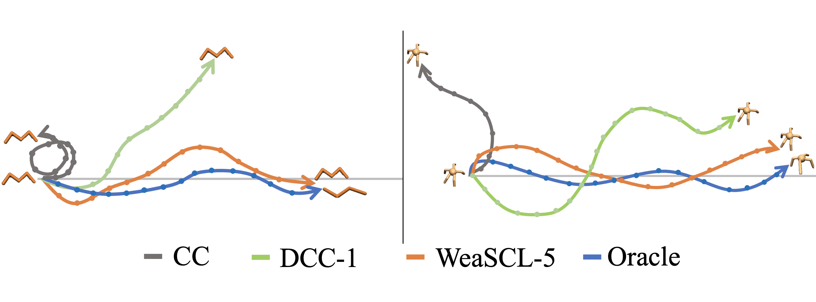
Figure 4: Sample trajectories for 4-link swimmer (left) and 5-legged ant (right). The grey line is the positive x-axis, which direction the robot is supposed to move toward. The oracle is only available in $\mathcal{M}^{2}$ (3-link swimmer and 4-legged ant).

Simulated Robots. As shown in Fig. 5, we create two dynamics in the simulated Panda Robot: the original 7-DoF robot arm, and a 5-DoF arm that fixes the third and forth joints of the 7-DoF arm (shown by red crosses). We define the paired abstractions based on the end-effector position in the state (green arrows) or the joint force in the action (purple arrows). We test two settings of paired abstractions: (1) only using the end-effector position ($Y^{s}$); (2) using both the end-effector position and the joint force ($Y^{s}$ and $Y^{a}$). Our goal is to translate the policy from 5-DoF to 7-DoF.

We show our results in Table III. We observe that WeaSCL-5 outperforms the baselines, DCC-1 and CC. WeaSCL-5 also outperforms the variants: WeaSCL-1 and DCC-5, which demonstrates the efficacy of both kinds of weak supervisions. We also note that WeaSCL-5 with $Y^{s}$ and $Y^{a}$ outperforms WeaSCL-5 with $Y^{s}$, which demonstrates that WeaSCLcan handle similarities over multiple abstractions elegantly and having access to similarities over multiple types of abstractions improves the performance.

Figure 5: Demonstrating the two robot arms with different degrees of freedom and the paired abstractions of end-effector positions and joint forces.

CC	-315.09$\pm$115.74
DCC-1	-255.33$\pm$160.19
DCC-5	-233.47$\pm$103.19
WeaSCL-1 ($Y^{s}$)	-225.28$\pm$100.39
WeaSCL-1 ($Y^{s}$ and $Y^{a}$)	-219.88$\pm$121.11
WeaSCL-5 ($Y^{s}$)	-78.43$\pm$22.06
WeaSCL-5 ($Y^{s}$ and $Y^{a}$)	-73.07 $\pm$42.19
Oracle	-20.68$\pm$21.30

TABLE III: The performance of the translated policy under different morphologies in the simulated robot environment.

V-B Cross-Physics

We conduct the experiments in Mujoco Hopper and Walker2d environments under a cross-physics setting, where we create different agents by varying the physical factors in the environment. We vary the gravitational constant in the Hopper environment and vary the friction of feet in the Walker2d environment. The exact value of the gravitational constant and the friction of the agent $\mathcal{M}^{1}$ and $\mathcal{M}^{2}$ are in Table IV. Note that only changing the physical parameters does not change the state and action spaces but changes the transition. Our goal is to translate a policy across environments with different physical parameters.

TABLE IV: Physical parameters in the Hopper and Walker2d.

Environment	Agent $\mathcal{M}^{2}$	Agent $\mathcal{M}^{1}$
		Setup1	Setup2
Hopper (Gravitational Constant)	9.8	0.5	5.0
Walker2d (Friction)	0.9	9.9	19.9

We use confidence as the abstraction to define similarity, where confidence lies in $[0,1]$ indicating how good a state, action pair is with respect to the reward function. For example, if a state, action pair always appears in optimal trajectories, we regard it as optimal and assign confidence $1$ to it. Then for all the state-action pairs in all trajectories, we randomly sample $1000$ pairs of state-action pairs with varying similarity as the dataset to learn the similarity function.

Here, we need trajectories with different confidence values for $\Xi^{1}$ and $\Xi^{2}$. For each environment and physical parameter, we train $7$ policies with different rewards, which range from the random policy to the optimal policy. We then collect $10$ trajectories from each policy as the trajectory set. We compute the reward for each trajectory and normalize the reward into $[0,1]$ by min-max normalization, where the normalized reward is used as the confidence for each trajectory. For each state-action pair in a trajectory, we use the trajectory confidence value as the confidence used for abstraction.

TABLE V: The performance of the transferred or translated policy under different physics.

Method	Gravity $0.5$	Gravity $5.0$	Friction $9.9$	Friction $19.9$
Direct	269.59$\pm$2.45	335.41$\pm$7.89	290.84$\pm$10.12	280.49$\pm$20.54
CC	61.19$\pm$39.91	83.26$\pm$155.79	178.93$\pm$219.81	236.15$\pm$72.39
DR	295.64$\pm$4.87	376.31$\pm$9.41	297.32$\pm$9.42	310.18$\pm$22.24
DCC-1	26.48$\pm$45.17	6.03$\pm$4.32	305.28$\pm$7.01	375.22$\pm$101.77
DCC-2	271.59$\pm$50.02	190.08$\pm$186.22	369.07$\pm$48.11	588.70$\pm$201.02
DCC-3	234.46$\pm$217.32	229.69$\pm$243.62	302.15$\pm$7.11	540.31$\pm$143.63
DCC-4	256.91$\pm$55.10	195.03$\pm$148.78	307.50$\pm$3.04	799.97$\pm$138.63
DCC-5	276.73 $\pm$120.39	231.76$\pm$161.27	305.11$\pm$4.62	598.56$\pm$219.53
WeaSCL-1	208.14$\pm$189.65	143.72$\pm$180.01	321.04$\pm$14.40	587.73$\pm$117.49
WeaSCL-2	325.80$\pm$57.06	279.33$\pm$107.24	499.52$\pm$48.99	1052.62$\pm$224.62
WeaSCL-3	137.49$\pm$132.33	387.12 $\pm$186.80	301.30$\pm$4.18	693.94$\pm$245.45
WeaSCL-4	129.05$\pm$84.62	283.38 $\pm$184.15	308.94$\pm$2.39	674.47$\pm$122.79
WeaSCL-5	130.09$\pm$75.48	272.69$\pm$91.31	306.67$\pm$6.30	550.24$\pm$202.03
Oracle	1952.99$\pm$32.41	3060.55$\pm$21.72	3604.38$\pm$52.59	1632.18$\pm$22.86

We show the results of our method and baselines in Table V. For DCC and our method, we report the results of using the dynamics cycle-consistency for $1-5$ steps, since the performance does not increase or even decrease for more than $5$ steps. We observe that our method with a proper number of steps for dynamics cycle-consistency achieves the best reward in all the tasks. Note that in most of the tasks, only two steps of dynamics cycle-consistency are sufficient to achieve the best performance, which demonstrates that the proposed approach is computationally efficient.

V-C Cross-Modality

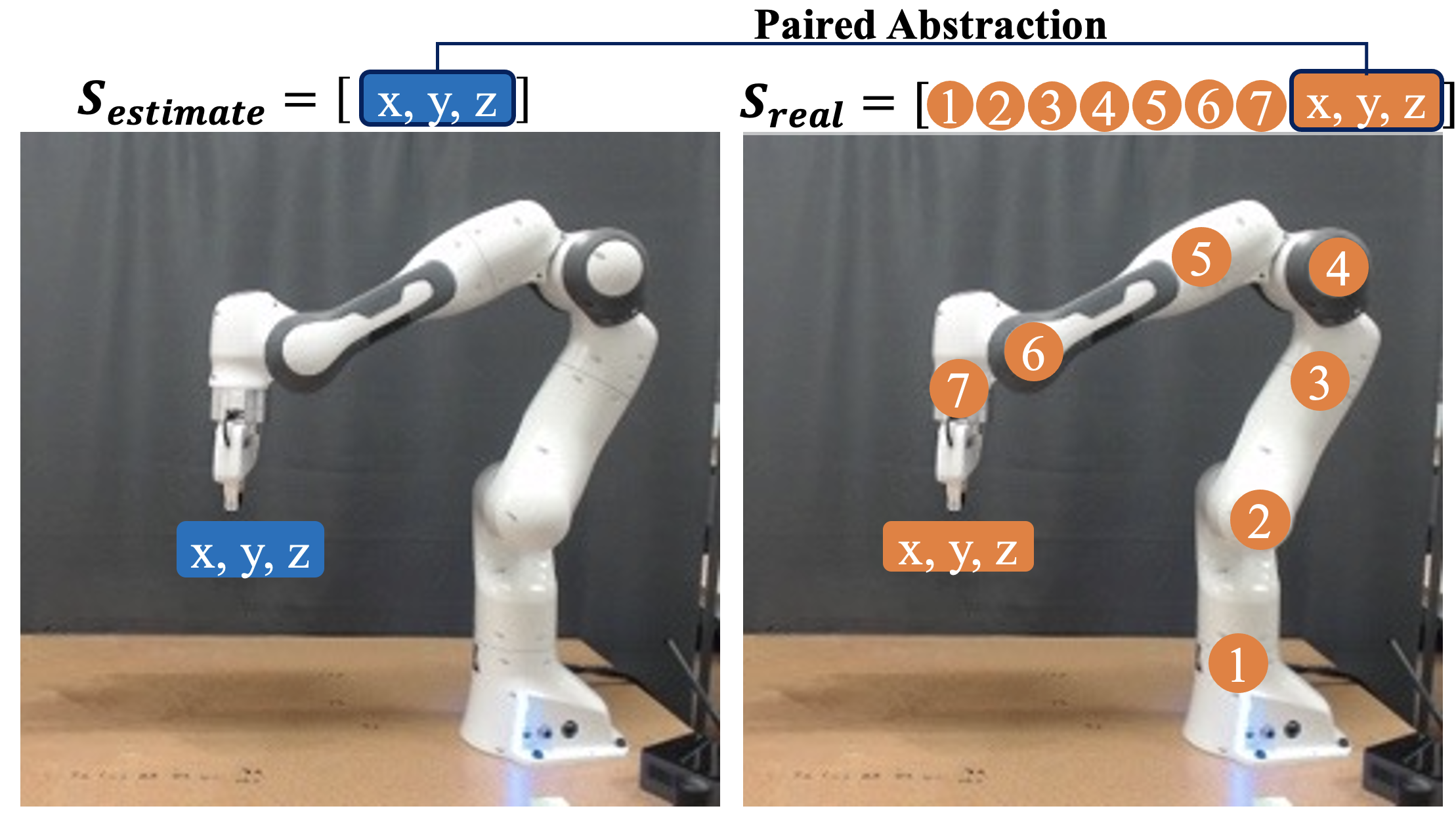
Figure 6: Top: An illustration of the real robot arm environments. Bottom: The norm of joint differences on the robot.

We also conduct experiments on the real robot under a cross-modality setting, where we translate across the visual observations and the joint states of a real Franka Panda robot arm. Our goal is to predict the state of the robot (joint configurations) from the visual observation of the robot. Our abstraction here is the end-effector pose of the robot in these two domains (ground-truth state and visual observations) and we collect $100$ similarity pairs to learn the similarity function.. Note that the actions are the same and we just need to learn the state map $\Phi$, which takes the RGB images as inputs and outputs the joint state of the robot.

As shown in Figure 6, WeaSCL-5 achieves the lowest estimation error compared to baselines CC and DCC-1 and also the variants DCC-5 and WeaSCL-1, which demonstrates the efficacy of our approach in real robot applications.

VI Conclusion

Summary. We propose a weakly supervised correspondence learning approach (WeaSCL) that leverages weak supervision in the form of temporal ordering and paired abstraction data. This eases the need for expensive paired data, and enables more accurate correspondence learning. Experiment results show that WeaSCL outperforms the state-of-the-art correspondence learning methods based on unpaired data.

Limitations and Future Work. Though we leverage the easy-to-access weak supervision to improve correspondence learning, this type of supervision still requires domain knowledge or human experts to annotate. In the future, we also plan to automatically detect the abstraction needed for weak supervision and reduce the size of the required annotation.

VII Acknowledgements

We would like to thank FLI grant RFP2-000, NSF Awards 1849952 and 1941722, and ONR for their support.

References

- [1] C. L. Nehaniv, K. Dautenhahn, et al., “The correspondence problem,” Imitation in animals and artifacts, vol. 41, 2002.
- [2] M. Nielsen, “12-month-olds produce others’ intended but unfulfilled acts,” Infancy, vol. 14, no. 3, pp. 377–389, 2009.
- [3] A. N. Meltzoff, “Understanding the intentions of others: re-enactment of intended acts by 18-month-old children.” Developmental psychology, vol. 31, no. 5, p. 838, 1995.
- [4] A. Gupta, C. Devin, Y. Liu, P. Abbeel, and S. Levine, “Learning invariant feature spaces to transfer skills with reinforcement learning,” arXiv preprint arXiv:1703.02949, 2017.
- [5] P. Sermanet, C. Lynch, Y. Chebotar, J. Hsu, E. Jang, S. Schaal, S. Levine, and G. Brain, “Time-contrastive networks: Self-supervised learning from video,” in 2018 IEEE international conference on robotics and automation (ICRA). IEEE, 2018, pp. 1134–1141.
- [6] A. H. Jha, S. Anand, M. Singh, and V. Veeravasarapu, “Disentangling factors of variation with cycle-consistent variational auto-encoders,” in Proceedings of the European Conference on Computer Vision (ECCV), 2018, pp. 805–820.
- [7] A. Zhang, R. T. McAllister, R. Calandra, Y. Gal, and S. Levine, “Learning invariant representations for reinforcement learning without reconstruction,” in International Conference on Learning Representations, 2021. [Online]. Available: https://openreview.net/forum?id=-2FCwDKRREu
- [8] J.-Y. Zhu, T. Park, P. Isola, and A. A. Efros, “Unpaired image-to-image translation using cycle-consistent adversarial networks,” in Proceedings of the IEEE international conference on computer vision, 2017, pp. 2223–2232.
- [9] A. Bansal, S. Ma, D. Ramanan, and Y. Sheikh, “Recycle-gan: Unsupervised video retargeting,” in Proceedings of the European conference on computer vision (ECCV), 2018, pp. 119–135.
- [10] L. Smith, N. Dhawan, M. Zhang, P. Abbeel, and S. Levine, “Avid: Learning multi-stage tasks via pixel-level translation of human videos,” arXiv preprint arXiv:1912.04443, 2019.
- [11] J. Hoffman, E. Tzeng, T. Park, J.-Y. Zhu, P. Isola, K. Saenko, A. Efros, and T. Darrell, “Cycada: Cycle-consistent adversarial domain adaptation,” in International conference on machine learning. PMLR, 2018, pp. 1989–1998.
- [12] S. James, P. Wohlhart, M. Kalakrishnan, D. Kalashnikov, A. Irpan, J. Ibarz, S. Levine, R. Hadsell, and K. Bousmalis, “Sim-to-real via sim-to-sim: Data-efficient robotic grasping via randomized-to-canonical adaptation networks,” in Proceedings of the IEEE/CVF Conference on Computer Vision and Pattern Recognition, 2019, pp. 12 627–12 637.
- [13] Q. Zhang, T. Xiao, A. A. Efros, L. Pinto, and X. Wang, “Learning cross-domain correspondence for control with dynamics cycle-consistency,” arXiv preprint arXiv:2012.09811, 2020.
- [14] M. Y. Zhang, Z. Huang, D. P. Paudel, J. Thoma, and L. Van Gool, “Weakly paired multi-domain image translation,” Proceedings BMVC 2020, 2020.
- [15] S. Shukla, L. Van Gool, and R. Timofte, “Extremely weak supervised image-to-image translation for semantic segmentation,” in 2019 IEEE/CVF International Conference on Computer Vision Workshop (ICCVW). IEEE, 2019, pp. 3368–3377.
- [16] F. Sadeghi and S. Levine, “Cad2rl: Real single-image flight without a single real image,” arXiv preprint arXiv:1611.04201, 2016.
- [17] J. Tobin, R. Fong, A. Ray, J. Schneider, W. Zaremba, and P. Abbeel, “Domain randomization for transferring deep neural networks from simulation to the real world,” in 2017 IEEE/RSJ international conference on intelligent robots and systems (IROS). IEEE, 2017, pp. 23–30.
- [18] X. B. Peng, M. Andrychowicz, W. Zaremba, and P. Abbeel, “Sim-to-real transfer of robotic control with dynamics randomization,” in 2018 IEEE international conference on robotics and automation (ICRA). IEEE, 2018, pp. 3803–3810.
- [19] W. Yan, A. Vangipuram, P. Abbeel, and L. Pinto, “Learning predictive representations for deformable objects using contrastive estimation,” arXiv preprint arXiv:2003.05436, 2020.
- [20] L. Pinto, M. Andrychowicz, P. Welinder, W. Zaremba, and P. Abbeel, “Asymmetric actor critic for image-based robot learning,” arXiv preprint arXiv:1710.06542, 2017.
- [21] O. M. Andrychowicz, B. Baker, M. Chociej, R. Jozefowicz, B. McGrew, J. Pachocki, A. Petron, M. Plappert, G. Powell, A. Ray, et al., “Learning dexterous in-hand manipulation,” The International Journal of Robotics Research, vol. 39, no. 1, pp. 3–20, 2020.
- [22] F. Ramos, R. C. Possas, and D. Fox, “Bayessim: adaptive domain randomization via probabilistic inference for robotics simulators,” arXiv preprint arXiv:1906.01728, 2019.
- [23] S. Zakharov, W. Kehl, and S. Ilic, “Deceptionnet: Network-driven domain randomization,” in Proceedings of the IEEE/CVF International Conference on Computer Vision, 2019, pp. 532–541.
- [24] Y. Wu, W. Yan, T. Kurutach, L. Pinto, and P. Abbeel, “Learning to manipulate deformable objects without demonstrations,” arXiv preprint arXiv:1910.13439, 2019.
- [25] B. Chen, A. Sax, G. Lewis, I. Armeni, S. Savarese, A. Zamir, J. Malik, and L. Pinto, “Robust policies via mid-level visual representations: An experimental study in manipulation and navigation,” arXiv preprint arXiv:2011.06698, 2020.
- [26] Y. Liu, A. Gupta, P. Abbeel, and S. Levine, “Imitation from observation: Learning to imitate behaviors from raw video via context translation,” in 2018 IEEE International Conference on Robotics and Automation (ICRA). IEEE, 2018, pp. 1118–1125.
- [27] M. E. Taylor and P. Stone, “Transfer learning for reinforcement learning domains: A survey.” Journal of Machine Learning Research, vol. 10, no. 7, 2009.
- [28] M. E. Taylor, P. Stone, and Y. Liu, “Transfer learning via inter-task mappings for temporal difference learning.” Journal of Machine Learning Research, vol. 8, no. 9, 2007.
- [29] H. B. Ammar, E. Eaton, P. Ruvolo, and M. E. Taylor, “Unsupervised cross-domain transfer in policy gradient reinforcement learning via manifold alignment,” in Twenty-Ninth AAAI Conference on Artificial Intelligence, 2015.
- [30] E. Tzeng, C. Devin, J. Hoffman, C. Finn, P. Abbeel, S. Levine, K. Saenko, and T. Darrell, “Adapting deep visuomotor representations with weak pairwise constraints,” in Algorithmic Foundations of Robotics XII. Springer, 2020, pp. 688–703.
- [31] G. Joshi and G. Chowdhary, “Cross-domain transfer in reinforcement learning using target apprentice,” in 2018 IEEE International Conference on Robotics and Automation (ICRA). IEEE, 2018, pp. 7525–7532.
- [32] K. Kim, Y. Gu, J. Song, S. Zhao, and S. Ermon, “Domain adaptive imitation learning,” in International Conference on Machine Learning. PMLR, 2020, pp. 5286–5295.
- [33] H. Bharadhwaj, Z. Wang, Y. Bengio, and L. Paull, “A data-efficient framework for training and sim-to-real transfer of navigation policies,” in 2019 International Conference on Robotics and Automation (ICRA), 2019, pp. 782–788.
- [34] T. Zhou, P. Krahenbuhl, M. Aubry, Q. Huang, and A. A. Efros, “Learning dense correspondence via 3d-guided cycle consistency,” in Proceedings of the IEEE Conference on Computer Vision and Pattern Recognition, 2016, pp. 117–126.
- [35] A. H. Liu, Y.-C. Liu, Y.-Y. Yeh, and Y.-C. F. Wang, “A unified feature disentangler for multi-domain image translation and manipulation,” arXiv preprint arXiv:1809.01361, 2018.
- [36] K. Bousmalis, A. Irpan, P. Wohlhart, Y. Bai, M. Kelcey, M. Kalakrishnan, L. Downs, J. Ibarz, P. Pastor, K. Konolige, et al., “Using simulation and domain adaptation to improve efficiency of deep robotic grasping,” in 2018 IEEE international conference on robotics and automation (ICRA). IEEE, 2018, pp. 4243–4250.
- [37] K. Rao, C. Harris, A. Irpan, S. Levine, J. Ibarz, and M. Khansari, “Rl-cyclegan: Reinforcement learning aware simulation-to-real,” in Proceedings of the IEEE/CVF Conference on Computer Vision and Pattern Recognition, 2020, pp. 11 157–11 166.
- [38] H. Sakoe and S. Chiba, “Dynamic programming algorithm optimization for spoken word recognition,” IEEE transactions on acoustics, speech, and signal processing, vol. 26, no. 1, pp. 43–49, 1978.
- [39] M. Rohrbach, S. Amin, M. Andriluka, and B. Schiele, “A database for fine grained activity detection of cooking activities,” in 2012 IEEE conference on computer vision and pattern recognition. IEEE, 2012, pp. 1194–1201.
- [40] Z.-H. Zhou, “A brief introduction to weakly supervised learning,” National science review, vol. 5, no. 1, pp. 44–53, 2018.
- [41] L. Lee, B. Eysenbach, R. Salakhutdinov, S. S. Gu, and C. Finn, “Weakly-supervised reinforcement learning for controllable behavior,” arXiv preprint arXiv:2004.02860, 2020.
- [42] H. Ma, Y. Wang, L. Tang, S. Kodagoda, and R. Xiong, “Towards navigation without precise localization: Weakly supervised learning of goal-directed navigation cost map,” arXiv preprint arXiv:1906.02468, 2019.
- [43] I. Goodfellow, J. Pouget-Abadie, M. Mirza, B. Xu, D. Warde-Farley, S. Ozair, A. Courville, and Y. Bengio, “Generative adversarial nets,” Advances in neural information processing systems, vol. 27, 2014.