Implications of Distance over Redistricting Maps: Central and Outlier Maps

Abstract

In representative democracy, a redistricting map is chosen to partition an electorate into a collection of districts each of which elects a representative. A valid redistricting map must satisfy a collection of constraints such as being compact, contiguous, and of almost equal population. However, these imposed constraints are still loose enough to enable an enormous ensemble of valid redistricting maps. This fact introduces a difficulty in drawing redistricting maps and it also enables a partisan legislature to possibly gerrymander by choosing a map which unfairly favors it. In this paper, we introduce an interpretable and tractable distance measure over redistricting maps which does not use election results and study its implications over the ensemble of redistricting maps. Specifically, we define a central map which may be considered as being "most typical" and give a rigorous justification for it by showing that it mirrors the Kemeny ranking in a scenario where we have a committee voting over a collection of redistricting maps to be drawn. We include run-time and sample complexity analysis for our algorithms, including some negative results which hold using any algorithm. We further study outlier detection based on this distance measure. More precisely, we show gerrymandered maps that lie very far away from our central maps in comparison to a large ensemble of valid redistricting maps. Since our distance measure does not rely on election results, this gives a significant advantage in gerrymandering detection which is lacking in all previous methods.

1 Introduction

Redistricting is the process of dividing an electorate into a collection of districts which each elect a representative. In the United States, this process is used for both federal and state-level representation, and we will use the U.S. House of Representatives as a running example throughout this paper. Subject to both state and federal law, the division of states into congressional districts is not arbitrary and must satisfy a collection of properties such as districts being contiguous and of near-equal population. Despite these regulations, it is clear that redistricting is vulnerable to strategic manipulation in the form of gerrymandering. The body in charge of redistricting can easily create a map within the legal constraints that leads to election results which favor a particular outcome (e.g., more representatives elected from one political party in the case of partisan gerrymandering). In addition, the ability to draw gerrymandered districts has improved greatly with the aid of computers since the historic salamander-shaped district approved by Massachusetts Governor Elbridge Gerry in 1812. For example, assuming voting consistent with the 2016 election, the state of North Carolina with 13 representatives can be redistricted to elect either 3 Democrats and 10 republicans or 10 Democrats and 3 Republicans.

However, despite this obvious threat to functioning democracy, partisan gerrymandering has often eluded regulation partly because it has been difficult to measure. In response, a recent line of research introduced sampling techniques to randomly generate a large collection of redistricting maps Chikina et al., (2017); DeFord et al., (2019); Herschlag et al., (2020) and calculate statistics such as a histogram of the number of seats won by each party using this collection. With these statistics, one can check if a proposed or enacted map is an outlier with respect to the sample. For example, the 2012 redistricting map of North Carolina produced $4$ seats for the democratic party whereas $95\%$ of the sampled maps led to between $6$ and $9$ seats Mattingly and Vaughn, (2014). In fact, these techniques were used as a key argument in the most recent U.S. Supreme Court case on gerrymandering Rucho v. Common Cause, (2019) and have supported successful efforts to change redistricting maps in state supreme court cases LWV vs Commonwealth of Pennsylvania, (2018). More importantly for the present work, at least two states, Michigan and Wisconsin, will use such a sampling tool DeFord et al., (2019) in the current redistricting process in response to the 2020 U.S. Census  Chen, (2021).

While great progress has been made in recent years on the problem of detecting/labeling possible gerrymandering through the use of these sampling techniques which can quantify outlier characteristics in a given map, the question of drawing a redistricting map in a way that is “fair” and immune to strategic manipulation remains largely unclear. We survey some existing proposals to automate redistricting in more detail in Section 2, but none of them have been adopted in practice thus far. The direction most commonly proposed by automated redistricting methods is to cast redistricting as a constrained optimization problem Cohen-Addad et al., (2018); Hettle et al., (2021); Liu et al., (2016), with objectives such as compactness and a collection of common constraints (district contiguity, equal population, etc.). However, formulating redistricting as an optimization problem poses an issue in the fact that there are multiple desired properties, and it is not clear why one should be optimized for over others.

Indeed, since there is a collection of redistricting maps that can be considered valid or legal, it seems quite reasonable to attempt to output the most “typical” map. Inspired by social choice theory (in particular, the Kemeny rule Kemeny, (1959); Brandt et al., (2016)), we propose a redistricting procedure in which the most typical (central) map among a given collection is selected. More precisely, we introduce a family of distance functions over redistricting maps and then select the map which minimizes the sum of distances to the other maps.

1.1 Our Contributions

We introduce the novel approach of choosing a central map among a set of redistricting maps and propose a method for identifying such a map. More concretely, we define a family of distances over redistricting maps and give algorithms that can find the medoid of a collection of given maps. Our family of distances is simple and interpretable and can accommodate various considerations such as the population of voting units or the distances between them (see Section 3.1). Further, we show a rigorous justification for choosing a central map based on a committee voting scenario. Specifically, the central map is the one that minimizes the sum of distances from the maps voted on, similar to Kemeny ranking Kemeny, (1959) (see Proposition 1).

En route to obtaining the medoid map we derive the centroid map which is not in fact a valid redistricting map, however has very interesting proprieties. Such as its $(i,j)$-entry being equal to the probability that voting units $i$ and $j$ are in the same district. Moreover, we show a simple linear-time algorithm for obtaining this centroid map which we do not think is obvious given the fact that the structures we deal with are rather complicated (redistricting maps). Moreover, under the assumption that we can sample valid maps in an independent and identically distributed manner, we derive the sample complexity for obtaining the centroid map.

Experimentally, we test our results over the states of North Carolina, Maryland, and Pennsylvania. Interestingly, we find that a by product of having a central map is a method for detecting gerrymandered maps. Concretely, the states of North Carolina and Pennsylvania have had enacted maps which were widely considered to be gerrymandered and in fact some were struck down by the state supreme court LWV vs Commonwealth of Pennsylvania, (2018). In response, some remedial maps were either suggested or enacted. We find that when we sample a large ensemble of redistricting maps and plot their distances from the centroid map, the gerrymandered maps have very large distances at the tail of the distribution whereas the remedial maps are much closer to the centroid. In fact, the gerrymandered maps we examined were all in at least the 99th percentile in terms of distance to the centroid. This perhaps suggests a new rule in drawing redistricting maps. Specifically, the drawn map should not be too faraway from the centroid.

2 Related Work

Less than a decade ago, several early works ushered in the current era of Markov Chain Monte Carlo (MCMC) sampling techniques for gerrymandering detection Mattingly and Vaughn, (2014); Wu et al., (2015); Fifield et al., (2015). Followup work has both refined these techniques and further analyzed their ability to approximate the target distribution. Authors of these works have been involved in court cases in Pennsylvania Chikina et al., (2017) and North Carolina Herschlag et al., (2020) with sampling approaches being used to demonstrate that existing maps were outliers as evidence of partisan gerrymandering. One of the most recent works in this area introduces the $\operatorname{\textbf{ReCom}}$ tool DeFord et al., (2019) which was used by the Wisconsin People’s Maps Commission and the Michigan Independent Citizens Redistricting Commission in the current redistricting cycle following the 2020 U.S. census Chen, (2021). Overall, these techniques have primarily been used to analyze and sometimes reject existing maps rather than draw new maps. However, we may think of them as at least narrowing the search space of maps drawn by legislatures. Along these lines, it has been shown that even the regulation of gerrymandering via outlier detection is subject to strategic manipulation Brubach et al., (2020).

On the automated redistricting side, many map drawing algorithms have favored optimization approaches and in particular, optimizing some notion of compactness while avoiding explicit use of partisan information. Approaches emphasizing compactness include balanced power diagrams Cohen-Addad et al., (2018), a $k$-median-based objective Bycoffe et al., (2018), and minimizing the number of cut edges in a planar graph Hettle et al., (2021). Some works include partisan information for the sake of creating competitive districts (districts with narrow margins between the two main parties). The PEAR tool Liu et al., (2016) balances nonpartisan criteria like compactness (defined by Polsby-Popper score Polsby and Popper, (1991)) with other criteria such as competitiveness and uses an evolutionary algorithm with some similarity to the random walks taken by MCMC sampling approaches. Other works go even further in the explicitly partisan direction. For example, Pegden et al., (2017) devises a game theoretic approach which aims to provide a map that is fair to the two dominant parties. Finally, there are methods which prefer simplicity such as the Splitline Ryan and Smith, (2022) algorithm which iteratively splits a state until the desired number of districts is reached.

In all of these approaches the aim is to automate redistricting, but it is difficult to determine whether the choices made are the “right” or “fairest” decisions. The question of whether optimizing properties such as compactness while ignoring partisan factors could result in partisan bias has been a concern for some time. Cho, (2019) notes a comment by Justice Scalia suggesting that such a process could be biased against Democratic voters clustered in cities in Vieth v. Jubelirer Vieth v. Jubelirer, (2004). For those that do take partisan bias into account, there are questions of whether purposely drawing competitive districts or giving a fair allocation to two parties are really beneficial to voters.

Finally, like Abrishami et al., (2020) we are introducing a distance measure over redistricting maps. However, our distance is easy to compute and does not require solving a linear program. Further, our focus is on the implications of having a distance measure, i.e. the medoid and centroid maps that will be introduced. Moreover, unlike Abrishami et al., (2020) we can detect gerrymandered maps rigorously by specifying where they lie on a distance histogram without using an embedding method and using $200,000$ samples instead of only $100$.

3 Problem Set-Up

A given state is modelled by a graph $G=(V,E)$ where each vertex $v\in V$ represents a voting block (unit). Each unit $v$ has a weight $w(v)>0$ which represents its population. Further, $\forall u,v\in V$ there is an edge $e=(u,v)\in E$ if and only if the two vertices are connected (geographically this means that units $u$ and $v$ share a boundary). The number of units is $|V|=n$. A redistricting (redistricting map or simply map) $M$ is a partition of $V$ into $k>0$ many districts, i.e., $V=V_{1}\cup V_{2}\dots\cup V_{k}$ where each $V_{i}$ represents a district and $\forall i\in[k],|V_{i}|\neq 0$ and $\forall i,j\in[k],V_{i}\cap V_{j}=\emptyset\ \text{if}\ i\neq j$. The redistricting map $M$ is decided by the induced partition, i.e., $M=\{V_{1},\dots,V_{k}\}$. For a redistricting $M$ to be considered valid, it must satisfy a collection of properties, some of which are specific to the given state. We use the most common properties as stated in DeFord et al., (2019); Hettle et al., (2021): (1) Compactness: The given partitioning should have “compact” districts. Although there is no definitive mathematical criterion which decides compactness for districts, some have used common definitions such as Polsby-Popper or Reock Score Alexeev and Mixon, (2018). Others have used a clustering criterion like the $k$-median objective Cohen-Addad et al., (2018) or considered the total number of cuts (number of edges between vertices in different districts) DeFord et al., (2019). (2) Equal Population: To satisfy the desideratum of “one person one vote” each district should have approximately the same number of individuals. I.e., a given district $V_{i}$ should satisfy $\sum_{v\in V_{i}}w(v)\in[(1-\epsilon)\frac{\sum_{v\in V}w(v)}{k},(1+\epsilon)\frac{\sum_{v\in V}w(v)}{k}]$ where $\epsilon$ is a non-negative parameter relaxing the equal population constraint. (3) Contiguity: Each district (partition) $V_{i}$ should be a connected component, i.e., $\forall i\in[k]$ and $\forall u,v\in V_{i}$, $v$ should be reachable from $u$ through vertices which only belong to $V_{i}$.

Our proofs do not rely on these properties and therefore can likely even accommodate further desired properties.

Let $\operatorname{\mathcal{M}}$ be the set of all valid maps. Let $\operatorname{\mathcal{D}}(\operatorname{\mathcal{M}})$ be a distribution over these maps. Furthermore, define a distance function over the maps $d:\operatorname{\mathcal{M}}\times\operatorname{\mathcal{M}}\rightarrow[0,\infty)$. Then the population medoid map is $M^{*}$ which is a solution to the following:

$$M^{*}=\operatorname*{arg\,min}\limits_{\operatorname{\mathnormal{M}}\in\operatorname{\mathcal{M}}}\ \underset{\operatorname{\mathnormal{M}}^{\prime}\sim\operatorname{\mathcal{D}}(\operatorname{\mathcal{M}})}{\operatorname{\mathbb{E}}}[d(\operatorname{\mathnormal{M}},\operatorname{\mathnormal{M}}^{\prime})]$$ (1)

In words, the population medoid map is a valid map minimizing the expected sum of distances away from all valid maps according to the distribution $\operatorname{\mathcal{D}}(\operatorname{\mathcal{M}})$. This serves as a natural way to define a central or most typical map with respect to a given distance metric of interest.

Since we clearly operate over a sample (a finite collection) from $\operatorname{\mathcal{D}}(\operatorname{\mathcal{M}})$; therefore, we assume that the following condition holds:

Condition 3.1.

We can sample maps from the distribution $\operatorname{\mathcal{D}}(\operatorname{\mathcal{M}})$ in an independent and identically distributed ($\operatorname{\textbf{iid}}$) manner in polynomial time.

We note that although independence certainly does not hold over the sampling methods of DeFord et al., (2019); Mattingly and Vaughn, (2014) since they use MCMC methods, it makes the derivations significantly more tractable. Further, the specific choice of the sampling technique is somewhat immaterial to our objective.

Based on the above condition, we can sample from the distribution $\operatorname{\mathcal{M}}$ efficiently and obtain a finite set of maps $\operatorname{\mathcal{M}_{\mathnormal{T}}}$ having $T$ many maps, i.e., $|\operatorname{\mathcal{M}_{\mathnormal{T}}}|=T$.

Now, we define the sample medoid, which is simply the extension of the population medoid, but restricted to the given sample. This leads to the following definition:

$$\bar{M}^{*}=\operatorname*{arg\,min}\limits_{\operatorname{\mathnormal{M}}\in\operatorname{\mathcal{M}_{\mathnormal{T}}}}\sum_{M^{\prime}\in\operatorname{\mathcal{M}_{\mathnormal{T}}}}\ d(\operatorname{\mathnormal{M}},\operatorname{\mathnormal{M}}^{\prime})$$ (2)

3.1 Distance over Redistricting Maps

Before we introduce a distance over maps, we note that a given map (partition) $M$ can be represented using an “adjacency” matrix $A$ in which $A(i,j)=1$ if and only if $\exists V_{\ell}\in M:i,j\in V_{\ell}$ otherwise $A(i,j)=0$. We note that this adjacency matrix can be seen as drawing an edge between every two vertices $i,j$ that are in the same district, i.e., where $A(i,j)=1$. It is clear that we can refer to a map by the partition $M$ or the induced adjacency matrix $A$. Accordingly, we refer to the population medoid as $M^{*}$ or $\operatorname{\mathnormal{A^{*}}}$ and the sample medoid as $\bar{M}^{*}$ or $\operatorname{\mathnormal{\bar{A}^{*}}}$

We now introduce our distance family which is parametrized by a weight matrix $\Theta$ and have the following form:

$$\operatorname{\mathnormal{d_{\Theta}}}(A_{1},A_{2})=\frac{1}{2}\sum_{i,j\in V}\theta(i,j)|A_{1}(i,j)-A_{2}(i,j)|$$ (3)

where we only require that $\theta(i,j)>0,\forall i,j\in V$ where $\theta(i,j)$ is the $(i,j)$ entry of $\Theta$. For the simple case where $\theta(i,j)=1,\forall i,j\in V$, our distance $d_{\textbf{1}}(A_{1},A_{2})$ is equivalent to a Hamming distance over adjacency matrices. When $\theta(i,j)=1,\forall i,j\in V$, we refer to the metric as the unweighted distance. We note that such a distance measure was used in previous work that considered adversarial attacks on clustering Chhabra et al., (2020); Cinà et al., (2022).

Another choice of $\Theta$ that leads to a meaningful metric is the population-weighted distance where $\theta(i,j)=w(i)w(j)$. This leads to $d_{W}(A_{1},A_{2})=\frac{1}{2}\sum_{i,j\in V}w(i)w(j)|A_{1}(i,j)-A_{2}(i,j)|$. The population-weighted distance takes into account the number of individuals being separated from one another when vertices $i$ and $j$ are separated from one another by assigning a cost of $w(i)w(j)$. By contrast, the unweighted distance assigns the same cost regardless of the population values and thus has a uniform weight over the separation of units immaterial of the populations which they include.

Another choice of metric which is meaningful, could be of the form $\theta(i,j)=f(l(i,j))$ where $l(i,j)$ is the length of a shortest path between $i$ and $j$ and $f(.)$ is a positive decreasing function such as $f(l(i,j))=e^{-l(i,j)}$. Such a metric would place a smaller penalty for separating vertices that are far away from each other. In Appendix A we discuss an edit distance interpretation of our distance and show its calculation over a simple example.

4 Justification for Choosing a Central Map

Connection to the Kemeny Rule:

We note that the Kemeny rule Kemeny, (1959); Brandt et al., (2016) is the main inspiration behind our proposed framework. More specifically, if we have a set of alternatives and each individual votes by ranking the alternatives, then the Kemeny rule gives a method for aggregating the resulting collection of rankings. This is done by introducing a distance measure over rankings (the Kendall tau distance Kendall, (1938)) and then choosing the ranking which minimizes the sum of distances away from the other rankings in the collection as the aggregate ranking.

Although we do not deal with rankings here, we follow a similar approach to the Kemeny rule as we introduce a distance measure over redistricting maps and choose the map which minimizes the sum of the distances as the aggregate map. In fact, recently there has been significant citizen engagement in drawing redistricting maps. For example, in the state of Maryland an executive order from the governor has established a web page to collect citizen submissions of redistricting maps Commission, (2021). If each member of a committee was to vote for exactly one map in the given submitted maps, then if we interpret the probability $p_{\operatorname{\mathnormal{M}}^{\prime}}$ for a map $\operatorname{\mathnormal{M}}^{\prime}\in\operatorname{\mathcal{M}}$ to be the number of votes it received from the total set of votes, then the medoid map $M^{*}$ (similar to the Kemeny ranking) would be the map which minimizes the weighted sum of distances from the set of maps voted on. We include this result as a proposition and its proof follows directly from the definition we gave above:

Proposition 1.

Suppose we have a committee of $\mathcal{T}$ many voters and that each voter votes for one map from a subset of all possible valid maps $\operatorname{\mathcal{M}}$, then given a map $\operatorname{\mathnormal{M}}^{\prime}$, if we assign it a probability $p_{\operatorname{\mathnormal{M}}^{\prime}}=\frac{\sum_{\tau=1}^{\mathcal{T}}v_{\tau,\operatorname{\mathnormal{M}}^{\prime}}}{\mathcal{T}}$ where $v_{\tau,\operatorname{\mathnormal{M}}^{\prime}}\in\{0,1\}$ is the vote of member $\tau$ for map $\operatorname{\mathnormal{M}}^{\prime}$, then the medoid map $M^{*}=\operatorname*{arg\,min}\limits_{\operatorname{\mathnormal{M}}\in\operatorname{\mathcal{M}}}\ \underset{\operatorname{\mathnormal{M}}^{\prime}\sim p_{\operatorname{\mathnormal{M}}^{\prime}}}{\operatorname{\mathbb{E}}}[d(\operatorname{\mathnormal{M}},\operatorname{\mathnormal{M}}^{\prime})]$ is the map that minimizes the sum of distances from the set of valid maps where the distance to each map is weighted by the total votes it receives.

Connection to Distance and Clustering Based Outlier Detection:

The medoid map by virtue of minimizing the sum of distances can be considered a central map. Accordingly, one may consider using the medoid map to test for gerrymandering in a manner similar to distance and clustering based outlier detection He et al., (2003); Knox and Ng, (1998). More specifically, given a large ensemble of maps, if the enacted map is faraway from the medoid in comparison to the ensemble then this suggests possible gerrymandering. In fact, we carry experiments on the states of North Carolina and Pennsylvania (both of which have had enacted maps which were considered gerrymandered) and we indeed find the gerrymandered maps to be faraway whereas the remedial maps are much closer in terms of distance.

5 Algorithms

We show our linear time algorithm for obtaining the sample medoid in subsection 5.1. In 5.2 we define the population centroid, derive sample complexity guarantees for obtaining it, and show that its $(i,j)$ entry equals the probability of having $i$ and $j$ in the same district. Finally, in 5.3 we discuss obtaining the population medoid. Specifically, we show that even for a simple one dimensional distribution an arbitrarily large sample is not sufficient for obtaining the population medoid.

First, before we introduce our algorithms we show that our distance family is indeed a metric, i.e. satisfies the properties of a metric:

Proposition 2.

For all $\Theta$ such that $\forall i,j,\theta(i,j)>0$, the following distance function is a metric.

$$\operatorname{\mathnormal{d_{\Theta}}}(A_{1},A_{2})=\frac{1}{2}\sum_{i,j\in V}\theta(i,j)|A_{1}(i,j)-A_{2}(i,j)|$$

5.1 Obtaining the Sample Medoid

We note that in general obtaining the sample medoid is not scalable since it usually takes quadratic time Newling and Fleuret, (2017) in the number of samples, i.e. $\Omega(T^{2})$. An $O(T^{2})$ run time can be easily obtained through a brute-force algorithm which for every map calculates the sum of the distances from other maps and then selects the map with the minimum sum. However, for our family of distances $\operatorname{\mathnormal{d_{\Theta}}}(.,.)$ we show that the medoid map is the closest map to the centroid map and show a simple algorithm that runs in $O(T)$ time for obtaining the sample medoid. The fundamental cause behind this speed up is an equivalence between the Hamming distance over binary vectors and the square of the Euclidean distance which is still maintained with our generalized distance. Before introducing the theorem we define $\operatorname{\mathnormal{d_{2,\Theta}}}(A_{1},A_{2})=\frac{1}{2}\sum_{i,j\in V}\theta(i,j)(A_{1}(i,j)-A_{2}(i,j))^{2}$ where the absolute has been replaced by a square. Now we state the decomposition theorem:

Theorem 5.1.

Given a collection of redistricting maps $A_{1},\dots,A_{T}$, the sum of distances of the maps from a fixed redistricting map $A^{\prime}$ equals the following:

$$\sum_{t=1}^{T}\operatorname{\mathnormal{d_{\Theta}}}(A_{t},A^{\prime}) =\sum_{t=1}^{T}\operatorname{\mathnormal{d_{2,\Theta}}}(A_{t},\bar{A}_{c})+T\operatorname{\mathnormal{d_{2,\Theta}}}(\bar{A}_{c},A^{\prime})$$ (4)

where $\bar{A}_{c}=\frac{1}{T}\sum_{t=1}A_{t}$.

Notice that the above theorem introduces the centroid map $\operatorname{\mathnormal{\bar{A}_{c}}}$ which is simply equal to the empirical mean of the adjacency maps. It should be clear that with the exception of trivial cases the centroid map $\operatorname{\mathnormal{\bar{A}_{c}}}$ is not a valid adjacency matrix, since despite being symmetric it would have fractional entries between $0$ and $1$. Hence, the centroid map also does not lead to a valid partition or districting. Moreover, we note that it is more accurate to call $\operatorname{\mathnormal{\bar{A}_{c}}}$ the sample centroid, as opposed to the population centroid $A_{c}$ (see subsection 5.2) which we would obtain with an infinite number of samples.

  Input: $\operatorname{\mathcal{M}_{\mathnormal{T}}}=\{A_{1},\dots,A_{T}\}$, $\Theta=\{\theta(i,j)>0,\forall i,j\in V\}$.

  1: Calculate the centroid map $\operatorname{\mathnormal{\bar{A}_{c}}}=\frac{1}{T}\sum_{t=1}^{T}A_{t}$.

   2: Pick the map $\bar{A}^{*}\in\operatorname{\mathcal{M}_{\mathnormal{T}}}$ which minimizes the $\operatorname{\mathnormal{d_{2,\Theta}}}$ distance from the centroid $\operatorname{\mathnormal{\bar{A}_{c}}}$, i.e. $\bar{A}^{*}=\operatorname*{arg\,min}_{A\in\operatorname{\mathcal{M}_{\mathnormal{T}}}}\operatorname{\mathnormal{d_{2,\Theta}}}(A,\operatorname{\mathnormal{\bar{A}_{c}}})$.

  return  $\bar{A}^{*}$

Algorithm 1 Finding the Sample Medoid

The above theorem leads to Algorithm 1 with the following remark:

Remark 1.

Algorithm 1 returns the correct sample medoid and runs in $O(T)$ time.

We note that calculating the sample medoid in algorithm 1 has no dependence on the generating method. Therefore, if a set of maps are produced through any mechanism and are considered to be representative and sufficiently diverse, then algorithm 1 can be used to obtain the sample medoid in time that is linear in the number of samples.

5.2 Sample Complexity for Obtaining the Population Centroid

In the previous section we introduced the sample centroid $\operatorname{\mathnormal{\bar{A}_{c}}}$ which is simply equal to the empirical mean that we get by taking the average of the adjacency matrices, i.e. $\operatorname{\mathnormal{\bar{A}_{c}}}=\frac{1}{T}\sum_{t=1}^{T}A_{t}$. We now consider the population centroid $\operatorname{\mathnormal{A_{c}}}=\lim_{T\rightarrow\infty}\sum_{t=1}^{T}A_{t}$. Clearly, by the law of large numbers Zubrzycki, (1972), we have $\operatorname{\mathnormal{A_{c}}}(i,j)=\operatorname{\mathbb{E}}[A(i,j)]$ . It is also clear that $\operatorname{\mathnormal{A_{c}}}$ has an interesting property, specifically the $(i,j)$-entry equals the probability that $i$ and $j$ are in the same district:

Proposition 3.

$\operatorname{\mathnormal{A_{c}}}(i,j)=\Pr[i\text{ and }j\text{ in the same district}]$.

Now we show that with a sufficient number of samples, the sample centroid converges to the population centroid entry-wise and in terms of the $\operatorname{\mathnormal{d_{2,\Theta}}}$ value. Specifically, we have the following proposition:

Proposition 4.

If we sample $T\geq\frac{1}{\epsilon^{2}}\ln{\frac{n}{\delta}}$ $\operatorname{\textbf{iid}}$ samples, then with probability at least $1-\delta$, we have that $\forall i,j\in V:|\operatorname{\mathnormal{\bar{A}_{c}}}(i,j)-\operatorname{\mathnormal{A_{c}}}(i,j)|\leq\epsilon$. Further, let $\kappa=\max_{i,j\in V}\sqrt{\theta(i,j)}$, if we have $T\geq\frac{\kappa n^{2}}{\epsilon}\ln{\frac{n}{\delta}}$ $\operatorname{\textbf{iid}}$ samples, then $\operatorname{\mathnormal{d_{2,\Theta}}}(\operatorname{\mathnormal{\bar{A}_{c}}},\operatorname{\mathnormal{A_{c}}})\leq\epsilon$ with probability at least $1-\delta$.

5.3 Obtaining the Population Medoid

Having found the sample centroid $\operatorname{\mathnormal{\bar{A}_{c}}}$ and shown that it is a good estimate of the population centroid $\operatorname{\mathnormal{A_{c}}}$, we now show that we can obtain a good estimate of the population medoid by solving an optimization problem. Specifically, assuming that we have the population centroid $\operatorname{\mathnormal{A_{c}}}$, then the population medoid is simply a valid redistricting map $A$ which has a minimum $\operatorname{\mathnormal{d_{2,\Theta}}}(A,\operatorname{\mathnormal{A_{c}}})$ value. This follows immediately from Theorem 5.1. More interestingly, we show in fact that this optimization problem is a constrained instance of the min $k$-cut problem:

Theorem 5.2.

Given the population centroid $\operatorname{\mathnormal{A_{c}}}$, the population medoid $\operatorname{\mathnormal{A^{*}}}$ can be obtained by solving a constrained min $k$-cut problem.

If we have a good estimate $\operatorname{\mathnormal{\bar{A}_{c}}}$ of the population centroid $\operatorname{\mathnormal{A_{c}}}$, then we can solve the above optimization using $\operatorname{\mathnormal{\bar{A}_{c}}}$ instead of $\operatorname{\mathnormal{A_{c}}}$ and obtain an estimate of the population medoid $\operatorname{\mathnormal{\bar{A}^{*}}}$ instead of the true population medoid $\operatorname{\mathnormal{A^{*}}}$ and bound the error of that estimate. The issue is that the min $k$-cut problem is NP-hard Goldschmidt and Hochbaum, (1994); Saran and Vazirani, (1995) . Further, the existing approximation algorithms assume non-negativity of the weights. Even if these approximation algorithms can be tailored to this setting, the additional constraints on the partition being a valid redistricting (each partition being contiguous, of equal population, and compact) make it quite difficult to approximate the objective. In fact, excluding the objective and focusing on the constraint alone, only the work of Hettle et al., (2021) has produced approximation algorithm for redistricting maps but has done that for the restricted case of grid graphs. Further, while there exists heuristics for solving min $k$-cut for redistricting maps they only scale to at most around $500$ vertices Validi and Buchanan, (2022).

Having shown the difficulty in obtaining the population medoid by solving an optimization problem, it is reasonable to wonder whether we can gain any guarantees about the population medoid by sampling. We show a negative result. Specifically, the theorem below shows that we cannot guarantee that we can estimate the sample medoid of a distribution with high probability by choosing a sampled map even if we sample an arbitrarily large number of maps. This implies as a corollary that the sample medoid does not converge to the population medoid in contrast to the centroid (see Proposition 4).

Theorem 5.3.

For any arbitrary $T$ many $\operatorname{\textbf{iid}}$ samples $\{A_{1},\dots,A_{T}\}$ there exists a distribution over a set of redistricting maps such that: (1) $\Pr[\min_{A\in\{A_{1},\dots,A_{T}\}}d(A,A^{*})\geq 0.331]\geq\frac{2}{3}$ and (2) $\Pr[\min_{A\in\{A_{1},\dots,A_{T}\}}f(A)\geq 1.1f(A^{*})]\geq\frac{2}{3}$ where $f(.)$ is the medoid cost function.

We therefore, use a heuristic to find the medoid as mentioned in section 6.

6 Experiments

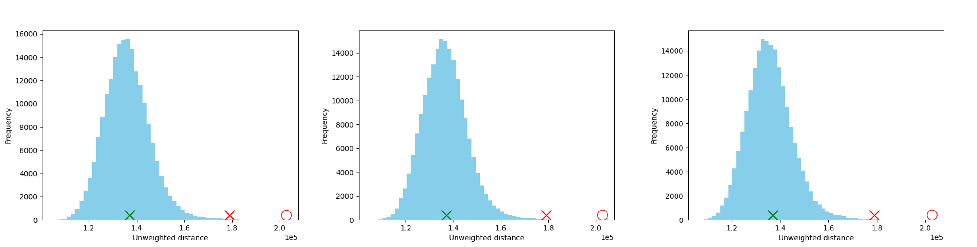
Figure 1: Distance histograms for NC using the unweighted distance measure. Different plots correspond to different seeds. For NC the distances of gerrymandered maps are indicated with red markers whereas the distances of the remedial maps are indicated with green markers (the ${\color[rgb]{1,0,0}\circ}$ and the X are for 2011 and 2016 enacted maps, respectively).

We conduct our experiments over 3 states. Specifically, North Carolina (NC), Maryland (MD), and Pennsylvania’s (PA). The number of voting units (vertices) and districts are around $2{,}700$, $1,{}800$, and $8{,}900$ for NC, MD, and PA, respectively. Further, the number of districts are $13$, $8$, and $18$ for NC, MD, and PA, respectively. Accordingly, PA is the largest state whereas MD is the smallest. He focus on the results for NC here and discuss the PA and MD results in Appendix C. We note that qualitatively all 3 states behave similarly. To generate a collection of maps, we use the Recombination algorithm $\operatorname{\textbf{ReCom}}$ from DeFord et al., (2019) whose implementation is available online. We note that $\operatorname{\textbf{ReCom}}$ is a Markov Chain Monte Carlo (MCMC) sampling method and hence the generated samples are not actually $\operatorname{\textbf{iid}}$. While this means that Condition (3.1) does not hold, we believe that our theorems still have utility and that future work can address more realistic sampling conditions. Moreover, we always exclude the first $2{,}000$ from any calculation as these are considered to be “burn-in” samples. Throughout this section when we say distance we mean $\operatorname{\mathnormal{d_{2,\Theta}}}(.,.)$ instead of $\operatorname{\mathnormal{d_{\Theta}}}(.,.)$. Further experimental results and figures are included in Appendix C.

Convergence of the Centroid:

We note that previous work such as DeFord et al., (2019); DeFord and Duchin, (2019) had used the $\operatorname{\textbf{ReCom}}$ algorithm for estimating statistics such as the histogram of election seats won by a party and has noted that using $50{,}000$ samples is sufficient for accurate results. However, our setting is more challenging. Specifically, the centroid includes $\Omega(n)$ entries where $n$ is the total number of voting units (vertices) whereas the election histogram includes only $k$ entries where $k$ is the number of districts and usually orders of magnitude smaller than the number of voting units. We sample $200{,}000$ maps instead to estimate the centroid. Here we emphasize the importance of our linear-time algorithm since using a quadratic-time algorithm on samples of the order of even $50{,}000$ could be computationally forbidding. Following similar practice to Herschlag et al., (2020) for verifying convergence, we repeat the procedure (sampling using $\operatorname{\textbf{ReCom}}$ and estimating the centroid) for a total of three times for each state where we start from a different seed map each time and verify that all three runs result in essentially the same centroid estimate.

To verify the closeness of the different centroid estimates, we calculate the distances between them and compare them to their distances from sampled redistricting maps using $\operatorname{\textbf{ReCom}}$. We find that the centroids are orders of magnitude closer to each other than to any other sampled map. For example, the maximum unweighted distance between any two centroids is less than $130$ whereas the minimum unweighted distance between any of the three centroids and any sampled map is more than $100,000$ which is three orders of magnitude higher. Similarly, the maximum weighted distance between any two centroids is less than $1.6\times 10^{9}$ whereas the mimimum weighted distance between a sampled amp and centroid is at least $1.3\times 10^{12}$ which is again three orders of magnitude higher.

Distance Histogram and Detecting Gerrymandered Maps:

For each state we plot the distance histogram from its centroid. More specifically, having estimated the centroid $\operatorname{\mathnormal{\bar{A}_{c}}}$, we sample $200{,}000$ maps and calculate $\operatorname{\mathnormal{d_{2,\Theta}}}(\operatorname{\mathnormal{\bar{A}_{c}}},A_{t})$ where $A_{t}$ is the $t^{\text{th}}$ sampled map. Figure 1 shows the unweighted distance histogram. The histogram appears like a normal distribution peaking at the middle (around the mean) and falling almost symmetrically away from the middle. This also indicates that while the centroid minimizes the sum of $\operatorname{\mathnormal{d_{2,\Theta}}}(\operatorname{\mathnormal{\bar{A}_{c}}},A_{t})$ distances, the maps do not actually concentrate around it as otherwise the histogram would have had a peak in the beginning at small distance values. Interestingly, the histogram has a similar shape for both distances (unweighted and weighted). Further, this shape of the histogram remains unchanged accross the different seeds.

Furthermore, previous work has used similar sampling methods to detect gerrymandered maps Chikina et al., (2017); Mattingly and Vaughn, (2014); Herschlag et al., (2020). In essence these paper demonstrate that the election outcome achieved by the enacted map is rare to happen in comparison to the large sampled ensemble of redistricting maps. Using similar logic, we find that we can also detect gerrymandered maps. Specifically, the 2011 and 2016 enacted maps of NC were widely considered to be gerrymandered and we find both maps to be at the right tail of the histogram and very faraway from the centroid. In contrast, to a remedial NC map that was drawn by a set of retired judges Herschlag et al., (2020) which is much closer to the centroid (see Figure 1 red and green marked points). Quite interestingly, all gerrymandered maps are in the 99th percentile in terms of distance (for both distance measures and across 3 seeds).

This suggests that we indeed have a method for detecting gerrymandered maps which in comparison to previous methods has the advantage of not needing election results (only a reasonable distance measure) and is very interpretable. Further, it is reasonable to consider this as setting a new rule when drawing redistricting maps or at least a guideline: the drawn map should not be very far away from the centroid. In Appendix C we show the histogram for PA and MD as well.

Finding the medoid:

We discuss the results for the unweighted distance. Since we have shown in subsection 5.3 that the medoid cannot be obtained by sampling, we follow a heuristic that consists of these steps: (1) Sample $200{,}000$ maps and pick the one closest to the centroid $A_{\text{closest}}$. (2) Start the $\operatorname{\textbf{ReCom}}$ chain from $A_{\text{closest}}$ but given a specific state (redistricting map) we only allow transitions to new states (maps) that are closer to the centroid and we do this for a total of $200{,}000$ steps to obtain the final estimated medoid $\hat{A}^{*}$. We follow this procedure three times one for each centroid . Figure 2 (top row) shows the $A_{\text{closest}}$ medoids from two different runs (each comparing to a different centroid). It is not difficult to see that they are different. The bottom row shows the final medoids after we run the chain from $A_{\text{closest}}$ to obtain $\hat{A}^{*}$. We see that the final medoids are indeed very similar and in fact when we measure the distances between them we find them to be very close.

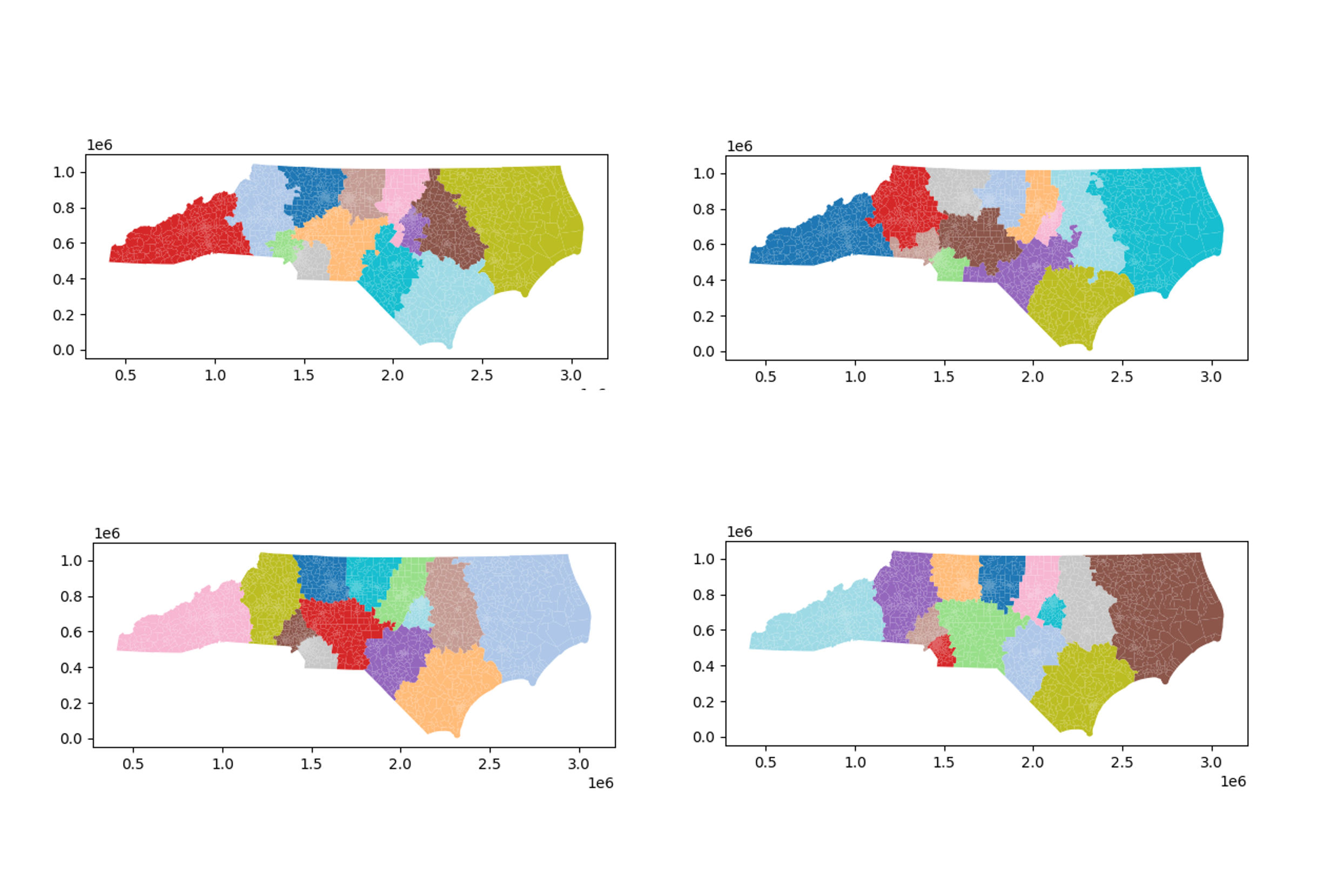
Figure 2: NC medoids, each column is for a specific seed. Top row: $A_{\text{closest}}$, Bottom row: $\hat{A}^{*}$.

7 Acknowledgements

The authors would like to thank Daniel Smolyak for many helpful discussions and the UMD CS Department for providing computational resources.

Appendix A Further Details About the Distance

Appendix B Omitted Proof

We restate the proposition and give its proof: See 1

Proof.

The first step in the proof follows from the definition of the weighted sum of distances for a map $M$ from the set of all maps:

$$M^{*} =\operatorname*{arg\,min}\limits_{\operatorname{\mathnormal{M}}\in\operatorname{\mathcal{M}}}\sum_{M^{\prime}\in\operatorname{\mathcal{M}}}\Big{[}\Big{(}\sum_{\tau}v_{\tau,\operatorname{\mathnormal{M}}}\Big{)}d(M,M^{\prime})\Big{]}$$

$$=\operatorname*{arg\,min}\limits_{\operatorname{\mathnormal{M}}\in\operatorname{\mathcal{M}}}\sum_{M^{\prime}\in\operatorname{\mathcal{M}}}\Big{[}\Big{(}\frac{\sum_{\tau}v_{\tau,\operatorname{\mathnormal{M}}}}{\mathcal{T}}\Big{)}d(M,M^{\prime})\Big{]}$$

$$=\operatorname*{arg\,min}\limits_{\operatorname{\mathnormal{M}}\in\operatorname{\mathcal{M}}}\sum_{M^{\prime}\in\operatorname{\mathcal{M}}}\Big{[}p_{\operatorname{\mathnormal{M}}}d(M,M^{\prime})\Big{]}$$

$$=\operatorname*{arg\,min}\limits_{\operatorname{\mathnormal{M}}\in\operatorname{\mathcal{M}}}\underset{\operatorname{\mathnormal{M}}^{\prime}\sim p_{\operatorname{\mathnormal{M}}^{\prime}}}{\operatorname{\mathbb{E}}}[d(\operatorname{\mathnormal{M}},\operatorname{\mathnormal{M}}^{\prime})]$$

∎

We restate the next proposition and give its proof: See 2

Proof.

Since $\theta(i,j)>0,\forall i,j\in V$, it is clear that $\operatorname{\mathnormal{d_{\Theta}}}(A_{1},A_{2})$ is non-negative, symmetric, and that it equals zero if and only if $A_{1}=A_{2}$. The triangle inequality follows since $|A_{1}(i,j)-A_{2}(i,j)|=|A_{1}(i,j)-A_{3}(i,j)+A_{3}(i,j)-A_{2}(i,j)|\leq|A_{1}(i,j)-A_{3}(i,j)|+|A_{3}(i,j)-A_{2}(i,j)|$, therefore we have:

$$\operatorname{\mathnormal{d_{\Theta}}}(A_{1},A_{2})=\frac{1}{2}\sum_{i,j\in V}\theta(i,j)|A_{1}(i,j)-A_{2}(i,j)|$$

$$\leq\frac{1}{2}\sum_{i,j\in V}\theta(i,j)\big{(}|A_{1}(i,j)-A_{3}(i,j)|+|A_{3}(i,j)-A_{2}(i,j)|\big{)}$$

$$\leq\frac{1}{2}\sum_{i,j\in V}\theta(i,j)|A_{1}(i,j)-A_{3}(i,j)|$$

$$\qquad+\frac{1}{2}\sum_{i,j\in V}\theta(i,j)|A_{3}(i,j)-A_{2}(i,j)|$$

$$=\operatorname{\mathnormal{d_{\Theta}}}(A_{1},A_{3})+\operatorname{\mathnormal{d_{\Theta}}}(A_{2},A_{3})$$

∎

We restate the next theorem and give its proof: See 5.1

Proof.

We begin with the following lemma:

Lemma 1.

For any $A_{1},A_{2}$ that are binary matrices (entries either $0$ or $1$), with $\operatorname{\mathnormal{d_{2,\Theta}}}(A_{1},A_{2})=\frac{1}{2}\sum_{i,j\in V}\theta(i,j)(A_{1}(i,j)-A_{2}(i,j))^{2}$, then we have that $\operatorname{\mathnormal{d_{\Theta}}}(A_{1},A_{2})=\operatorname{\mathnormal{d_{2,\Theta}}}(A_{1},A_{2})$.

Proof.

The proof is immediate since $A_{1}$ and $A_{2}$ are binary. ∎

It may seem redundant to introduce a new definition $\operatorname{\mathnormal{d_{2,\Theta}}}(.,.)$ since by Lemma 1, they are equivalent. However, we will shortly be using $\operatorname{\mathnormal{d_{2,\Theta}}}(.,.)$ over matrices which are not necessarily binary, clearly then we might have $\operatorname{\mathnormal{d_{\Theta}}}(A_{1},A_{2})\neq\operatorname{\mathnormal{d_{2,\Theta}}}(A_{1},A_{2})$.

We then introduce next lemma:

Lemma 2.

For any two matrices (not necessarily binary), the following holds:

$$\operatorname{\mathnormal{d_{2,\Theta}}}(A_{1},A_{2})=\frac{1}{2}\left\lVert A^{\Theta}_{1}-A^{\Theta}_{2}\right\rVert^{2}_{2}$$ (5)

where $A^{\Theta}_{s}(i,j)=\sqrt{\theta(i,j)}A_{s}(i,j),\forall s\in\{1,2\}$ and $\left\lVert A^{\Theta}_{1}-A^{\Theta}_{2}\right\rVert^{2}_{2}$ is the square of the $\ell_{2}$-norm of the vectorized form of the matrix $(A^{\Theta}_{1}-A^{\Theta}_{2})$.

Proof.

$$\operatorname{\mathnormal{d_{2,\Theta}}}(A_{1},A_{2}) =\frac{1}{2}\sum_{i,j\in V}\theta(i,j)(A_{1}(i,j)-A_{2}(i,j))^{2}$$

$$=\frac{1}{2}\sum_{i,j\in V}(\sqrt{\theta(i,j)}A_{1}(i,j)-\sqrt{\theta(i,j)}A_{2}(i,j))^{2}$$

$$=\frac{1}{2}\left\lVert A^{\Theta}_{1}-A^{\Theta}_{2}\right\rVert^{2}_{2}$$

∎

With the lemmas above, we can now prove the decomposition theorem:

$$\sum_{t=1}^{T}\operatorname{\mathnormal{d_{\Theta}}}(A_{t},A^{\prime}) =\sum_{t=1}^{T}\operatorname{\mathnormal{d_{2,\Theta}}}(A_{t},A^{\prime})\ \ \ \ \ \ \text{(using Lemma \ref{ham_eq_l2})}$$

$$=\sum_{t=1}^{T}\frac{1}{2}\left\lVert A^{\Theta}_{t}-{A^{\prime}}^{\Theta}\right\rVert^{2}_{2}\ \ \ \ \ \ \text{(using Lemma \ref{vector_lemma})}$$

$$=\frac{1}{2}\sum_{t=1}^{T}\left\lVert A^{\Theta}_{t}-\operatorname{\mathnormal{\bar{A}^{\Theta}_{c}}}+\operatorname{\mathnormal{\bar{A}^{\Theta}_{c}}}-{A^{\prime}}^{\Theta}\right\rVert^{2}_{2}$$

$$=\frac{1}{2}\sum_{t=1}^{T}\Big{[}(A^{\Theta}_{t}-\operatorname{\mathnormal{\bar{A}^{\Theta}_{c}}}+\operatorname{\mathnormal{\bar{A}^{\Theta}_{c}}}-{A^{\prime}}^{\Theta})^{\intercal}(A^{\Theta}_{t}-\operatorname{\mathnormal{\bar{A}^{\Theta}_{c}}}+\operatorname{\mathnormal{\bar{A}^{\Theta}_{c}}}-{A^{\prime}}^{\Theta})\Big{]}$$

$$=\sum_{t=1}^{T}\frac{1}{2}\Big{[}\left\lVert A^{\Theta}_{t}-\operatorname{\mathnormal{\bar{A}^{\Theta}_{c}}}\right\rVert^{2}_{2}+\left\lVert\operatorname{\mathnormal{\bar{A}^{\Theta}_{c}}}-{A^{\prime}}^{\Theta}\right\rVert^{2}_{2}\Big{]}+\left(\sum_{t=1}^{T}(A^{\Theta}_{t}-\operatorname{\mathnormal{\bar{A}^{\Theta}_{c}}})\right)^{\intercal}(\operatorname{\mathnormal{\bar{A}^{\Theta}_{c}}}-{A^{\prime}}^{\Theta})$$

$$=\sum_{t=1}^{T}\frac{1}{2}\left\lVert A^{\Theta}_{t}-\operatorname{\mathnormal{\bar{A}^{\Theta}_{c}}}\right\rVert^{2}_{2}+\frac{T}{2}\left\lVert\operatorname{\mathnormal{\bar{A}^{\Theta}_{c}}}-{A^{\prime}}^{\Theta}\right\rVert^{2}_{2}+(T\operatorname{\mathnormal{\bar{A}^{\Theta}_{c}}}-T\operatorname{\mathnormal{\bar{A}^{\Theta}_{c}}})^{\intercal}(\operatorname{\mathnormal{\bar{A}^{\Theta}_{c}}}-{A^{\prime}}^{\Theta})$$

$$=\sum_{t=1}^{T}\operatorname{\mathnormal{d_{2,\Theta}}}(A_{t},\operatorname{\mathnormal{\bar{A}_{c}}})+T\operatorname{\mathnormal{d_{2,\Theta}}}(\operatorname{\mathnormal{\bar{A}_{c}}},A^{\prime})$$

Note that in the fourth line we take the dot product with the matrices being in vectorized form and that $\operatorname{\mathnormal{\bar{A}^{\Theta}_{c}}}=\frac{1}{T}\sum_{t=1}^{T}A^{\Theta}_{t}$. Note that it follows that $\operatorname{\mathnormal{\bar{A}^{\Theta}_{c}}}(i,j)=\sqrt{\theta(i,j)}\operatorname{\mathnormal{\bar{A}_{c}}}(i,j)$. ∎

We restate the next proposition and give its proof: See 3

Proof.

By definition of the redistricting adjacency matrices and condition (3.1) for $\operatorname{\textbf{iid}}$ sampling we have that:

$$\operatorname{\mathnormal{A_{c}}}(i,j)=\underset{A_{t}\sim\operatorname{\mathcal{M}}}{\operatorname{\mathbb{E}}}[A_{t}(i,j)]$$

$$=(1)\Pr[i\text{ and }j\text{ are in the same district}]+(0)\Pr[i\text{ and }j\text{ are not in the same district}]$$

$$=\Pr[i\text{ and }j\text{ are in the same district}]$$

∎

We restate the next proposition and give its proof: See 4

Proof.

For a given $i,j\in V$ by the Hoeffding bound we have that:

$$\Pr[|\operatorname{\mathnormal{\bar{A}_{c}}}(i,j)-\operatorname{\mathnormal{A_{c}}}(i,j)|\leq\epsilon]\geq 1-2e^{-2\epsilon^{2}T}$$

$$\geq 1-2e^{-2\epsilon^{2}\frac{1}{\epsilon^{2}}\ln{\frac{n}{\delta}}}\geq 1-2(e^{2\ln{\frac{n}{\delta}}})^{-1}\geq 1-2\frac{\delta^{2}}{n^{2}}$$

Now we calculate the following event:

$$\Pr(\{\forall i,j\in V:|\operatorname{\mathnormal{\bar{A}_{c}}}(i,j)-\operatorname{\mathnormal{A_{c}}}(i,j)|\leq\epsilon\})$$

$$=1-\Pr(\{\exists i,j\in V:|\operatorname{\mathnormal{\bar{A}_{c}}}(i,j)-\operatorname{\mathnormal{A_{c}}}(i,j)|>\epsilon\})$$

$$\geq 1-\sum_{i,j\in V}2\frac{\delta^{2}}{n^{2}}\geq 1-2\delta^{2}\frac{(\frac{n^{2}-n}{2})}{n^{2}}\geq 1-\delta^{2}\geq 1-\delta\ \ \ \ \ \ \text{( since $\delta\in(0,1)$)}$$

Now we prove the second part. By applying the previous result with $\epsilon$ set to $\frac{\sqrt{\epsilon}}{\sqrt{\rho}n}$, we get that with probability at least $1-\delta$, $|\operatorname{\mathnormal{\bar{A}_{c}}}(i,j)-\operatorname{\mathnormal{A_{c}}}(i,j)|\leq\frac{\sqrt{\epsilon}}{\sqrt{\rho}n^{2}}$. It follows that:

$$\operatorname{\mathnormal{d_{2,\Theta}}}(\operatorname{\mathnormal{\bar{A}_{c}}},\operatorname{\mathnormal{A_{c}}}) =\frac{1}{2}\sum_{i,j\in V}\theta(i,j)(\operatorname{\mathnormal{\bar{A}_{c}}}(i,j)-\operatorname{\mathnormal{A_{c}}}(i,j))^{2}$$

$$\leq\frac{1}{2}\sum_{i,j\in V}\theta(i,j)\Big{(}\frac{\sqrt{\epsilon}}{\sqrt{\rho}n}\Big{)}^{2}\leq\frac{1}{2}\sum_{i,j\in V}\frac{\epsilon}{n^{2}}$$

$$\leq\frac{1}{2}\frac{\epsilon}{n^{2}}\frac{n^{2}-n}{2}\leq\epsilon$$

∎

We restate the next theorem and give its proof: See 5.2

Proof.

From Theorem 5.1, the population medoid is a valid redistricting map $A$ for which $\operatorname{\mathnormal{d_{2,\Theta}}}(A,\operatorname{\mathnormal{A_{c}}})$ is minimized. Note that since $A$ is a redistricting map, unlike $\operatorname{\mathnormal{A_{c}}}$ it must be a binary matrix. Therefore, $|A(i,j)-\operatorname{\mathnormal{A_{c}}}(i,j)|=(1-\operatorname{\mathnormal{A_{c}}}(i,j))+(2\operatorname{\mathnormal{A_{c}}}(i,j)-1)(1-A(i,j))$, where this identity can be verified by plugging 0 or 1 for $A(i,j)$ and seeing that it leads to an equality. Define the matrix $B$ as a “complement” of $A$. Specifically, $B(i,j)=1-A(i,j)$. It follows that $B(i,j)=1$ if and only if $i$ and $j$ are in different partitions and $B(i,j)=0$ otherwise. Clearly, $B$ is a binary matrix. We can obtain the following:

$$\operatorname{\mathnormal{d_{2,\Theta}}}(A,\operatorname{\mathnormal{A_{c}}})=\frac{1}{2}\sum_{i,j\in V}\theta(i,j)(A(i,j)-\operatorname{\mathnormal{A_{c}}}(i,j))^{2}$$

$$\quad=\frac{1}{2}\sum_{i,j\in V}\theta(i,j)\big{(}(1-\operatorname{\mathnormal{A_{c}}}(i,j))+(2\operatorname{\mathnormal{A_{c}}}(i,j)-1)(1-A(i,j))\big{)}^{2}$$

$$\quad=\frac{1}{2}\sum_{i,j\in V}\theta(i,j)\big{(}(1-\operatorname{\mathnormal{A_{c}}}(i,j))+(2\operatorname{\mathnormal{A_{c}}}(i,j)-1)B(i,j)\big{)}^{2}$$

$$\quad=\frac{1}{2}\sum_{i,j\in V}\theta(i,j)\big{(}(1-\operatorname{\mathnormal{A_{c}}}(i,j))^{2}+2(1-\operatorname{\mathnormal{A_{c}}}(i,j))(2\operatorname{\mathnormal{A_{c}}}(i,j)-1)B(i,j)+(2\operatorname{\mathnormal{A_{c}}}(i,j)-1)^{2}B^{2}(i,j)\big{)}$$

$$\quad=\frac{1}{2}\sum_{i,j\in V}\theta(i,j)\big{(}(1-\operatorname{\mathnormal{A_{c}}}(i,j))^{2}+2(1-\operatorname{\mathnormal{A_{c}}}(i,j))(2\operatorname{\mathnormal{A_{c}}}(i,j)-1)B(i,j)+(2\operatorname{\mathnormal{A_{c}}}(i,j)-1)^{2}B(i,j)\big{)}$$

$$\quad=\Big{[}\frac{1}{2}\sum_{i,j\in V}\theta(i,j)(\operatorname{\mathnormal{A_{c}}}^{2}(i,j)-2\operatorname{\mathnormal{A_{c}}}(i,j)+1)\Big{]}-\Big{[}\frac{1}{2}\sum_{i,j\in V}\theta(i,j)\big{(}1-2\operatorname{\mathnormal{A_{c}}}(i,j)\big{)}B(i,j)\Big{]}$$

Note that the first sum in the last equality is a constant and has no dependence on $B$. Hence to minimize $\operatorname{\mathnormal{d_{2,\Theta}}}(A,\operatorname{\mathnormal{A_{c}}})$, we maximize the following:

$$\max_{B} \sum_{i,j\in V}s(i,j)B(i,j)$$ (6)

s.t. $$B\text{ is a $k$ partition that leads to a valid redistricting map}$$ (7)

where the weight $s(i,j)$ is equal to $s(i,j)=\frac{1}{2}\theta(i,j)\big{(}1-2\operatorname{\mathnormal{A_{c}}}(i,j)\big{)}$. Clearly, this is a constrained max $k$-cut instance where the partition has to be a valid redistricting map.

∎

Theorem 5.3 shows a negative result for obtaining the population medoid of a set of redistricting maps. Before we show its proof, we show the following theorem which proves a similar result over points in a 2-dimensional Euclidean space. We note that both theorems hold even if the population (true) medoid is sampled with non-zero probability:

Theorem B.1.

There exists a distribution over a set of points $\mathcal{P}$ in the 2-dimensional Euclidean space such that given $T$ many $\operatorname{\textbf{iid}}$ samples $\{x_{1},\dots,x_{T}\}$ the following holds: (1) If $T\geq\text{poly}(\epsilon,\ln(1/\rho))$ then with probability at least $1-\rho$ we have $\left\lVert\frac{1}{T}\sum_{t=1}x_{t}-\operatorname{\mathbb{E}}[x]\right\rVert^{2}_{2}\leq\epsilon$. However, it is also the case that for any number of samples $T$, we have: (2) $\Pr[\min_{x\in\{x_{1},\dots,x_{T}\}}d(x,x^{*})\geq 0.999]\geq\frac{2}{3}$ and (3) $\Pr[\min_{x\in}f(x)\geq 1.2f(x^{*})]\geq\frac{2}{3}$ where $x^{*}$ is the population medoid and $f(.)$ is the medoid cost function.

Proof.

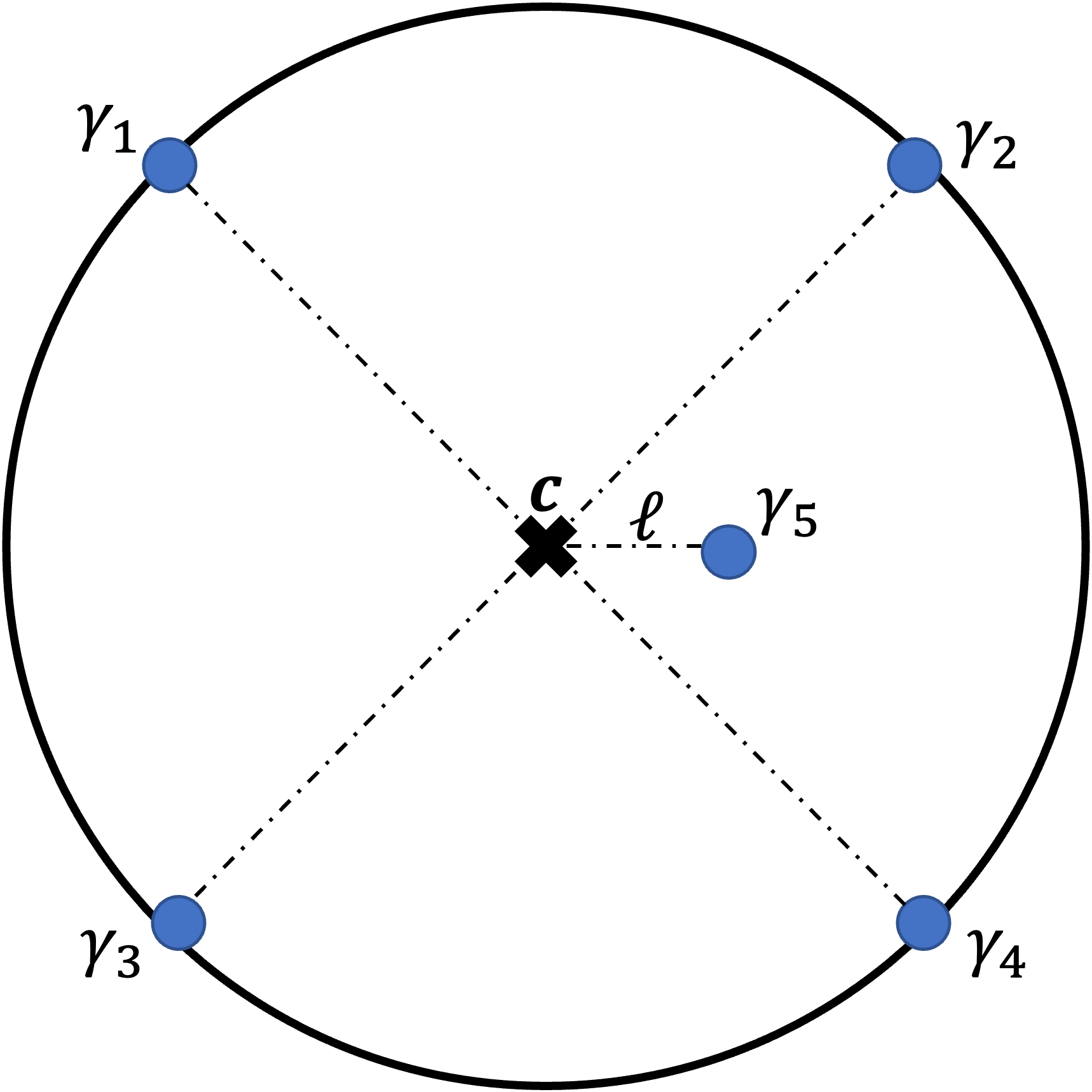
Figure 3: Points $\gamma_{1},\gamma_{2},\gamma_{3}$, and $\gamma_{4}$ all lie on the circle and the angle between any two adjacent points is $90^{\circ}$. Point $\gamma_{5}$ is a distance $\ell$ from the circle center $c$. The center $c$ is also the origin point of the 2-$d$ plane $(0,0)$.

Consider the set of points $\mathcal{P}=\{\gamma_{1},\gamma_{2},\gamma_{3},\gamma_{4},\gamma_{5}\}$ shown in Figure 3. Specifically, points $\gamma_{1},\gamma_{2},\gamma_{3}$ and $\gamma_{4}$ lie on a circle of radius $1$ at an equal separation. Point $\gamma_{5}$ lies closer to the center of the circle $c$ at a distance of $\ell$. Further, each point $\gamma_{i}$ has a probability $p_{i}$ of being sampled. Specifically, $p_{5}=\delta$ and $p_{1}=p_{2}=p_{3}=p_{4}=\frac{1-\delta}{4}$.

The centroid of the distribution is the expected value, i.e. $\operatorname{\mathbb{E}}[x]=\sum_{j=1}^{5}p_{j}\gamma_{j}$. It is straightforward to show that given $\operatorname{\textbf{iid}}$ samples $\{x_{1},x_{2},\dots,x_{T}\}$ where $T=\Omega(\frac{\ln(1/\rho)}{\epsilon})$, then $\left\lVert\frac{1}{T}\sum_{t=1}^{T}\hat{x}_{t}-\operatorname{\mathbb{E}}[x]\right\rVert^{2}_{2}\leq\epsilon$ with probability at least $1-\rho$. This follows by applying the generalized Hoeffding inequality (see Ashtiani et al., (2016) for example). This proves the first statement.

Now, given a candidate medoid point $\gamma^{\prime}$, the medoid cost function is $f(\gamma^{\prime})=\sum_{j=1}^{5}p_{j}d(\gamma^{\prime},\gamma_{j})$. Note that the medoid is the value of $\gamma^{\prime}$ which minimizes $f(\gamma^{\prime})$ and also $\gamma^{\prime}$ must be an element of the set, i.e. $\gamma^{\prime}\in\mathcal{P}$. It is easy to verify that $f(\gamma_{1})=\frac{1-\delta}{4}[d(\gamma_{1},\gamma_{1})+d(\gamma_{1},\gamma_{2})+d(\gamma_{1},\gamma_{3})+d(\gamma_{1},\gamma_{4})]+\delta d(\gamma_{1},\gamma_{5})>\frac{1-\delta}{4}[0+2\sqrt{2}+2]=\frac{1-\delta}{2}(1+\sqrt{2})$. By symmetry it also follows that $f(\gamma_{2}),f(\gamma_{3}),f(\gamma_{4})$ are each lower bounded by $\frac{1-\delta}{2}(1+\sqrt{2})$.

On the other hand, we have $f(\gamma_{5})=\frac{1-\delta}{4}\sum_{j=1}^{4}d(\gamma_{5},\gamma_{j})\leq\frac{1-\delta}{4}\sum_{j=1}^{4}[d(\gamma_{5},c)+d(c,\gamma_{j})]\leq\frac{1-\delta}{4}(4(1+\ell))=(1-\delta)(1+\ell)$. Further, for any $i\neq 5:\frac{f(\gamma_{i})}{f(\gamma_{5})}\geq\frac{\frac{1-\delta}{2}(1+\sqrt{2})}{(1-\delta)(1+\ell)}=\frac{(1+\sqrt{2})}{2(1+\frac{1}{1000})}>1.2$ by setting $\ell=\frac{1}{1000}$, and therefore $\gamma_{5}$ is the medoid. Further, $\forall i\in\{1,2,3,4\}:d(\gamma_{i},\gamma_{5})\geq d(\gamma_{i},c)-d(c,\gamma_{5})\geq 1-\ell\geq 0.999$. Therefore, to prove the second and third statements it is sufficient to prove that $\gamma_{5}$ would be sampled with probability at most $\frac{1}{3}$ in $T$ many $\operatorname{\textbf{iid}}$ samples:

$$\Pr[\text{Sampling $\gamma_{5}$ in $T$ $\operatorname{\textbf{iid}}$ samples}]$$

$$=1-\Pr[\text{Not sampling $\gamma_{5}$ in $T$ $\operatorname{\textbf{iid}}$ samples}]$$

$$=1-(1-\delta)^{T}\leq\frac{1}{3}$$

$$\iff\delta\leq 1-\sqrt[T]{\frac{2}{3}}$$

Therefore, by setting $\delta\leq 1-\sqrt[T]{\frac{2}{3}}$ the distribution satisfies all three statement simultaneously. ∎

Now we restate Theorem 5.3 and show its proof: See 5.3

Proof.

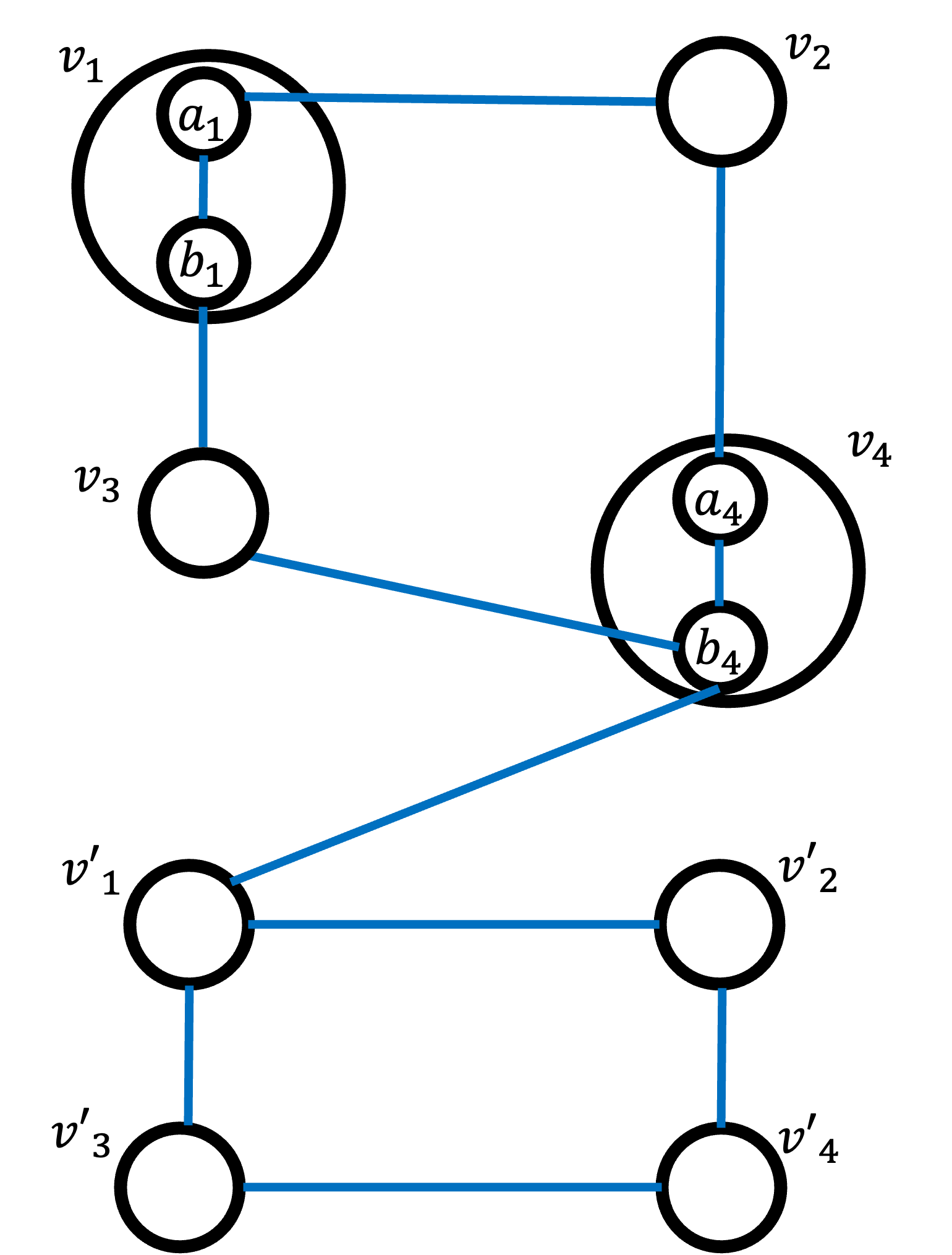
Figure 4: The graph shows a hypothetical state. Blue edges indicate that the vertices are adjacent geographically. All vertices have a weight (population) of 1, except for states $\{a_{1},b_{1},a_{4},b_{4}\}$ which have a weight of $\frac{1}{2}$.

Consider the hypothetical state shown in Figure 4 where vertices $v_{1}$ and $v_{4}$ are further subdividing into two vertices each. We wish to divide the state into $2$ districts ($k=2$). Since each vertex has a weight of $1$, except vertices $\{a_{1},b_{1},a_{4},b_{4}\}$ which each have a weight of $\frac{1}{2}$, then each district should have a population of $2$ to enforce the equal population rule with a tolerance less than $0.25$.

Denoting the set of all vertices by $V$ and letting $V^{\prime}=\{a_{1},b_{1},a_{4},b_{4}\}$, then the weight parameters of our weighted distance measure are defined as follows:

$$\theta(i,j)=\begin{cases}\epsilon&\text{if $i\ \&\ j\in V^{\prime}$}\\ \frac{1}{2}&\text{if $i\in V-V^{\prime},j\in V^{\prime}$ or $i\in V^{\prime},j\in V-V^{\prime}$}\\ 1&\text{otherwise}\end{cases}$$

Figure 5: Maps $M_{1},M_{2},M_{3}$, and $M_{4}$. Vertices in the same district are connected with edges.

Where $0<\epsilon\leq 1$. Now, consider the maps $M_{1},M_{2},M_{3}$, and $M_{4}$ shown in Figure 5. Based on the definition of the weighted distance measure, it is not difficult to see that given maps $M_{s}$ and $M_{t}$, then $\operatorname{\mathnormal{d_{\Theta}}}(M_{s},M_{t})$ can be computed visually by drawing the adjacent graphs of $M_{s}$ and $M_{t}$ and then finding the minimum number of edges that have to be deleted and added to $M_{s}$ to produce $M_{t}$ and adding the weighted $\theta(i.j)$ of these edges. By following this procedure, we can show that $\operatorname{\mathnormal{d_{\Theta}}}(M_{1},M_{3})=6+4\epsilon$ for example as shown in Figure 6. Here we list all distances:

$$\operatorname{\mathnormal{d_{\Theta}}}(M_{1},M_{2})=4$$

$$\operatorname{\mathnormal{d_{\Theta}}}(M_{1},M_{4})=\operatorname{\mathnormal{d_{\Theta}}}(M_{2},M_{4})=2+4\epsilon$$

$$\operatorname{\mathnormal{d_{\Theta}}}(M_{1},M_{3})=\operatorname{\mathnormal{d_{\Theta}}}(M_{2},M_{4})=(2+4\epsilon)+4=6+4\epsilon$$

$$\operatorname{\mathnormal{d_{\Theta}}}(M_{3},M_{4})=4$$

Given a map $M$, the medoid cost function is defined as $f(M)=\sum_{M^{\prime}\in\operatorname{\mathcal{M}}}p_{M^{\prime}}d(M,M^{\prime})$. Let the probabilities for the redistricting maps be assigned as follows: $p_{1}=p_{2}=p_{3}=\frac{1-\delta}{3}$ whereas $\Pr[\text{Sampling a Map $M\notin\{M_{1},M_{2},M_{3}\}$}]=\delta>0$. Accordingly, $p_{5}\leq\delta$.

Further, since $\theta(i,j)\leq 1\ ,\forall i,j\in V$, then maximum distance between any redistricting maps $D$ can be upper bounded by the highest number of edges that can be deleted and added from one map to produce another, therefore $D\leq 2{|V|\choose 2}=|V|(|V|-1)=10\times 9=90$ since $|V|=10$ (see Figure 4). The medoid cost function can be lower bounded for $M_{1},M_{2},$ and $M_{3}$ and upper bounded for $M_{4}$ as shown below:

$$f(M_{1})>\frac{1-\delta}{3}[d(M_{1},M_{2})+d(M_{1},M_{3})]=\frac{1-\delta}{3}(10+4\epsilon)$$

$$f(M_{2})>\frac{1-\delta}{3}[d(M_{1},M_{2})+d(M_{2},M_{3})]=\frac{1-\delta}{3}(10+4\epsilon)$$

$$f(M_{3})>\frac{1-\delta}{3}[d(M_{1},M_{3})+d(M_{2},M_{3})]=\frac{1-\delta}{3}(12+8\epsilon)$$

$$f(M_{4})<\frac{1-\delta}{3}[d(M_{1},M_{4})+d(M_{2},M_{4})+d(M_{3},M_{4})]+\delta D=\frac{1-\delta}{3}(8+8\epsilon)+90\delta\leq\frac{1-\delta}{3}(9+8\epsilon)$$

Where the last inequality was obtained by setting $\delta<\frac{1}{271}$ since it follows that $90\delta<\frac{1-\delta}{3}$. From the above bounds it follows that the population medoid cannot cannot be $M_{1},M_{2}$, or $M_{3}$.

Set $\epsilon=\frac{1}{1000}$ and $\delta\leq\frac{1}{1000}<\frac{1}{271}$ and with $1-(p_{1}+p_{2}+p_{3})=\delta$, then $\frac{1-\delta}{3}(1-4\epsilon)>0.331$ and $\frac{(10+4\epsilon)}{(9+8\epsilon)}>1.11$. With the population medoid denoted by $M^{*}$, then we have: $\min\limits_{i\in\{1,2,3\}}\frac{f(M_{i})}{f(M^{*})}\geq\min\limits_{i\in\{1,2,3\}}\frac{f(M_{i})}{f(M_{4})}\geq\frac{\frac{1-\delta}{3}(10+4\epsilon)}{\frac{1-\delta}{3}(9+8\epsilon)}>1.11$. Further, it follows by the triangle inequality that $\forall i\in\{1,2,3\}:f(M_{i})\leq f(M^{*})+d(M_{i},M^{*})$, thus $d(M_{i},M^{*})\geq\frac{1-\delta}{3}(1-4\epsilon)$, since otherwise $f(M^{*})+d(M_{i},M^{*})\leq f(M_{4})+d(M_{i},M^{*})<\frac{1-\delta}{3}(9+8\epsilon)+\frac{1-\delta}{3}(1-4\epsilon)=\frac{1-\delta}{3}(10+4\epsilon)$ which would be a contradiction.

From the above we have shown that, $\forall i\in\{1,2,3\}:d(M_{i},M^{*})\geq\frac{1-\delta}{3}(1-4\epsilon)>0.331$ and $\min\limits_{i\in\{1,2,3\}}\frac{f(M_{i})}{f(M^{*})}\geq 1.11$, therefore to prove parts (1) and (2) of the theorem it is sufficient to upper bound the probability of sampling a map that is not in $\{M_{1},M_{2},M_{3}\}$ in $T$ iid samples by $\frac{1}{3}$. This leads to the following:

$$\Pr[\text{Obtaining a map $M\notin\{M_{1},M_{2},M_{3}\}$ in a given $T$ $\ \operatorname{\textbf{iid}}$ samples}]$$

$$=1-\Pr[\text{No map $M\in\{M_{1},M_{2},M_{3}\}$ in the given $T$ $\ \operatorname{\textbf{iid}}$ samples}]$$

$$=1-(1-\delta)^{T}\leq\frac{1}{3}$$

Therefore, from the above we should have $\delta=\min\{\frac{1}{1000},1-\sqrt[T]{\frac{2}{3}}\}$ to satisfy both parts of the theorem.

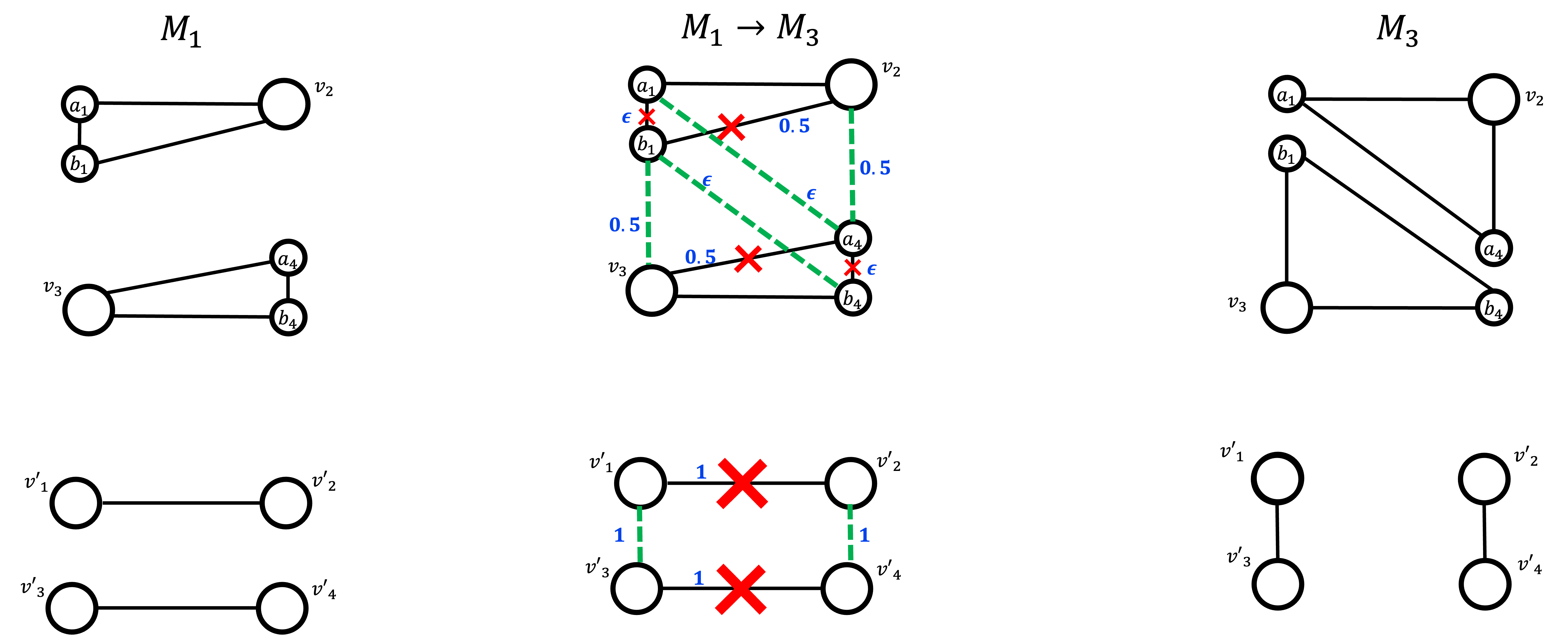
Figure 6: The first map is $M_{1}$ and the last is $M_{3}$. The middle map shows the edges the should be deleted from $M_{1}$ (marked with X) and the edges should be added to $M_{1}$ (dashed green edges) to produce $M_{3}$. The weight of each edge that is deleted or added is shown next to it in blue. By adding the weights we get that $\operatorname{\mathnormal{d_{\Theta}}}(M_{1},M_{3})=6+4\epsilon$.

∎

Remark:

In both theorems B.1 and 5.3 the probability of “failure” is set to $\frac{2}{3}$ but this is arbitrary as we can make it arbitrarily large by choosing smaller values of $\delta$. But our objective was simply to show that not sampled map would converge to the population medoid or would have a medoid cost function value that converges to the value of medoid cost function of the population medoid. Further, both theorems would hold if the population medoid is sampled with probability zero, but in our proofs we allowed the population medoid to be sampled with non-zero probability to show that the negative result would still hold even if we were to assume that the population medoid is sampled with non-zero probability.

Appendix C Additional Experimental Results

C.1 Convergence to the centroid

As a reminder to further test the robustness of our results and see the convergence, all calculations are done 3 times for each state, each time starting from a specific seed map. For example, we estimate the centroid three times, by sampling starting from seed maps $s_{1}$, $s_{2}$, and $s_{3}$ and as a result we end up with three centroids $c_{1}$, $c_{2}$, and $c_{3}$. Here we further verify the convergence of the centroids by showing that the final estimated centroids are close to each other. In fact, if we denote the smallest $\operatorname{\mathnormal{d_{2,\Theta}}}(.,.)$ distance between a sampled map and any of the centroids $c_{1}$, $c_{2}$, or $c_{3}$ by $\operatorname{\mathnormal{d_{2,\Theta}}}_{\min}$. Then we consistently find –for all states (NC,PA,MD) and all distance measures (unweighted and population-weighted)– that for any two estimated centroids $c_{i}$ and $c_{j}$ that $\operatorname{\mathnormal{d_{2,\Theta}}}(c_{i},c_{j})\leq\operatorname{\mathnormal{d_{2,\Theta}}}_{\min}$ by at least $2$ or $3$ orders of magnitude. This is strong evidence that while the differences in the estimation may be large in value, they are very small relative to the distances between other maps. Therefore, at this scale the estimation error is small. We note moreover the while we used $200,000$ samples to estimate the centroids for NC, we use only $50,000$ for PA and MD in each seed run and interestingly find that $50,000$ samples are sufficient. Table 1 shows the maximum $\operatorname{\mathnormal{d_{2,\Theta}}}(.,.)$ distance between any two estimated centroid and $\operatorname{\mathnormal{d_{2,\Theta}}}_{\min}$.

Table 1: Maximum Distance Between Any Two Centroids vs Minimum Distance between a Centroid and a Sampled Map

STATE	Distance Measure	$\max\limits_{i,j\in\{1,2,3\}}\operatorname{\mathnormal{d_{2,\Theta}}}(c_{i},c_{j})$	$\operatorname{\mathnormal{d_{2,\Theta}}}_{\min}$
NC	Unweighted	$1.2051\times 10^{2}$	$1.051030\times 10^{5}$
NC	Population-Weighted	$1.5446\times 10^{9}$	$1.333014\times 10^{12}$
PA	Unweighted	$5.0794\times 10^{3}$	$1.099175\times 10^{6}$
PA	Population-Weighted	$1.1090\times 10^{10}$	$2.036627\times 10^{12}$
MD	Unweighted	$2.5067\times 10^{2}$	$5.033550\times 10^{4}$
MD	Population-Weighted	$2.7067\times 10^{9}$	$5.015410\times 10^{11}$

C.2 Distance Histograms and Detecting Gerrymandered Maps

Here we produce the histogram maps for all states and all distance measures. Each histogram is produced for a given state and distance measure starting from a specific centroid and by sampling from its corresponding seed, e.g. we sample maps starting from seed $s_{1}$ and calculate $\operatorname{\mathnormal{d_{2,\Theta}}}(M,c_{1})$ between a sampled map $M$ and centroid $c_{1}$ to construct one histogram. We find similar observations to Figure 1, indeed we see that the shape of the histograms is stable across all states, distances, and centroids. I.e., all of the distance histograms peak in the middle and fall away from the middle similar to a normal distribution. Further, our observations about the gerrymandered maps of NC (Figure 7) still hold. In addition, we show similar observations in PA where we find that the gerrymandered map that was struck down by the state supreme court LWV vs Commonwealth of Pennsylvania, (2018) is an outlier in terms of distance. On the other hand, the remedial map has a much smaller distance and appears near the peak of the histogram.

Tables 2, 3, 4, and 5 list percentile distances for the above mentioned maps in NC and PA according to both unweighted and weighted distance measures. We see that the three gerrymander maps (the 2016 and 2011 enacted maps for NC and the 2011 enacted map for PA) are all above the 99th percentile for both distance measures and all three seeds. On the other hand, the NC Judge’s map and PA remedial map are near the peak of the histogram. In addition, the percentiles for these maps are fairly consistent across seeds for any given combination of state and distance measure.

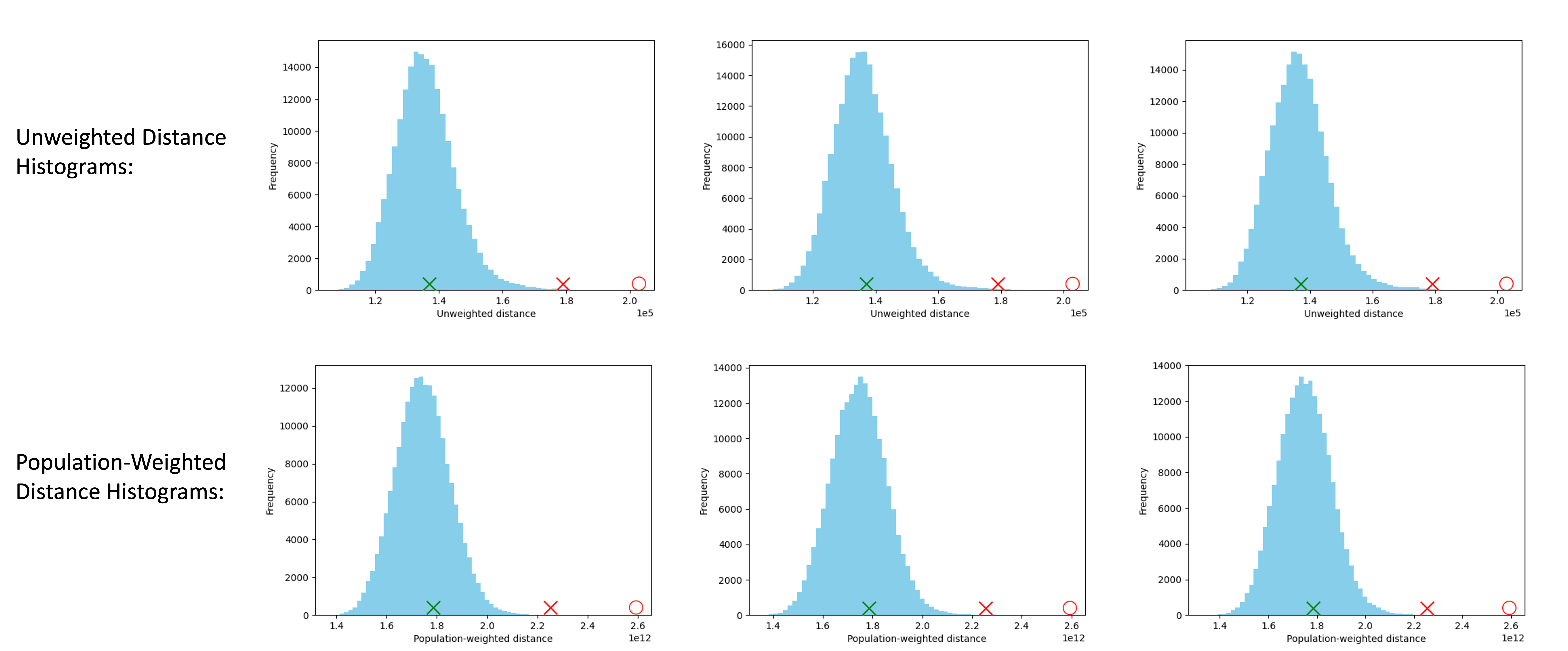
Figure 7: Distance histograms for NC, the distances of gerrymandered maps are indicated with red markers whereas the distances of the remedial maps are indicated with green markers. The ${\color[rgb]{1,0,0}\circ}$ and the X are for 2011 and 2016 enacted maps, respectively.

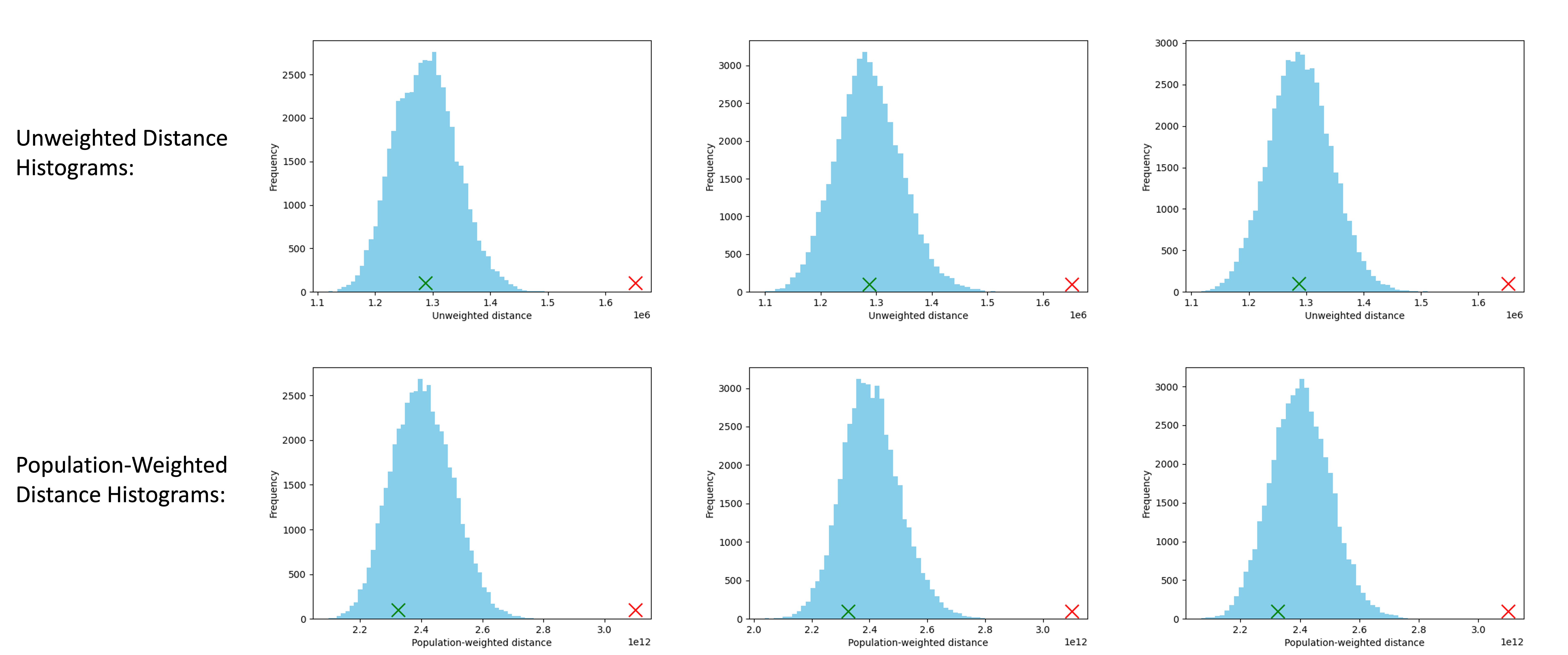
Figure 8: Distance histograms for PA, the distances of gerrymandered maps are indicated with red markers whereas the distances of the remedial maps are indicated with green markers..

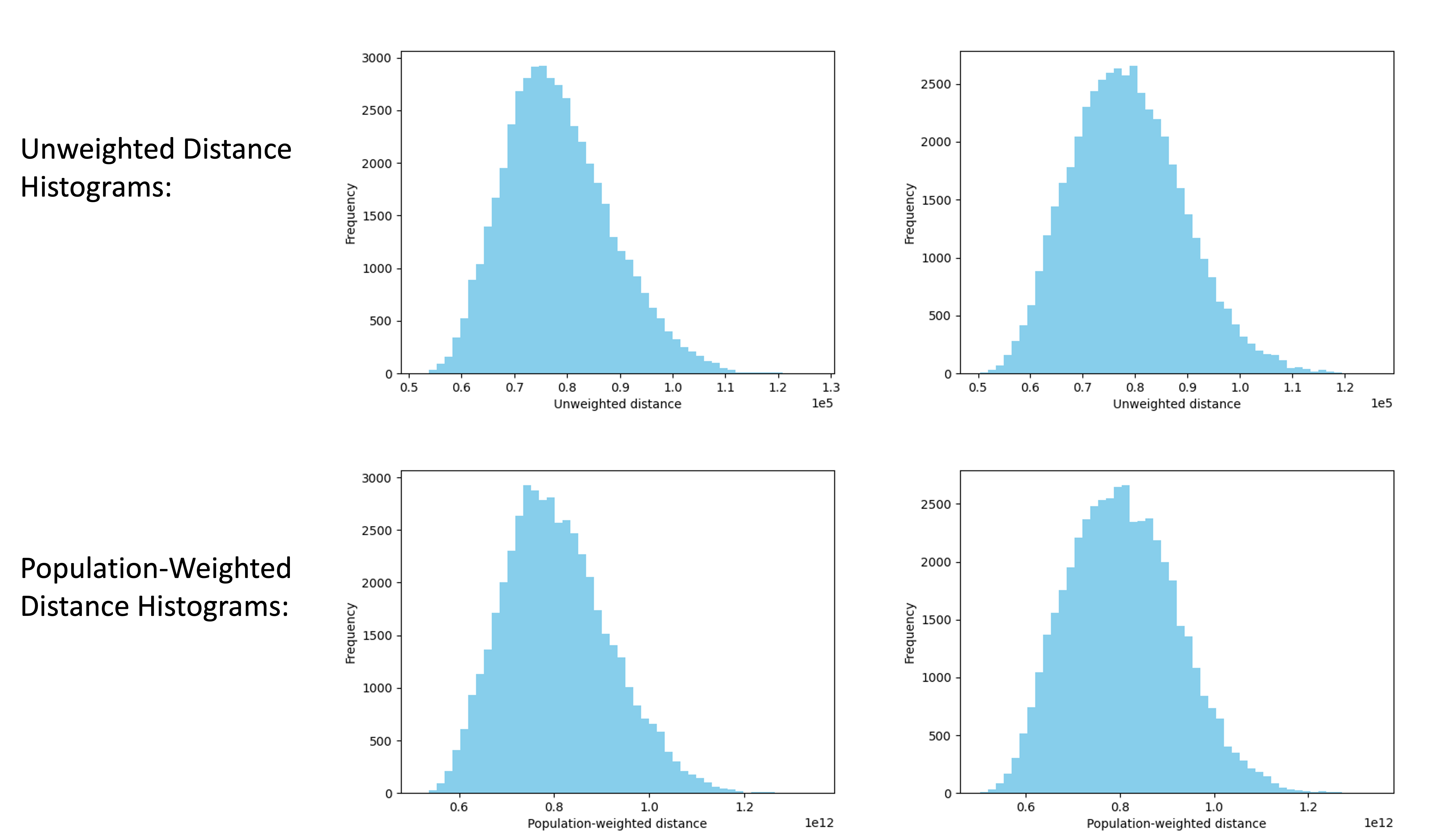
Figure 9: Distance histograms for MD.

Table 2: Percentile distances for special maps in NC using the unweighted distance measure.

Starting Seed	Judges’ map	2016 enacted map	2011 enacted map
Seed 1	58.362	99.942	100.0
Seed 2	57.004	99.927	100.0
Seed 3	54.558	99.943	100.0

Table 3: Percentile distances for special maps in NC using the weighted distance measure.

Starting Seed	Judges’ map	2016 enacted map	2011 enacted map
Seed 1	65.359	99.999	100.0
Seed 2	64.454	99.997	100.0
Seed 3	63.238	99.996	100.0

Table 4: Percentile distances for special maps in PA using the unweighted distance measure.

Starting Seed	Remedial map	2011 enacted map
Seed 1	49.992	100.0
Seed 2	51.875	100.0
Seed 3	48.715	100.0

Table 5: Percentile distances for special maps in PA using the weighted distance measure.

Starting Seed	Remedial map	2011 enacted map
Seed 1	22.383	100.0
Seed 2	20.956	100.0
Seed 3	21.813	100.0

Remark (distance from centroid is closely related to the average distance from the ensemble):

It is also worthwhile to point out the following interpretation about the distance from the centroid. Here we show that the distance from the centroid is a direct measure of the average distance from the ensemble of maps. This follows by direct manipulation of the decomposition theorem 5.1:

$$\operatorname{\mathnormal{d_{2,\Theta}}}(\mathnormal{\hat{M}_{1}},\operatorname{\mathnormal{\bar{A}_{c}}})=\underbrace{\frac{1}{T}\sum_{t=1}^{T}\operatorname{\mathnormal{d_{\Theta}}}(\mathnormal{\hat{M}_{1}},A_{t})}_{\text{Average distance between map $\mathnormal{\hat{M}_{1}}$ and the ensemble}}-\underbrace{\frac{1}{T}\sum_{t=1}^{T}\operatorname{\mathnormal{d_{2,\Theta}}}(A_{t},\operatorname{\mathnormal{\bar{A}_{c}}})}_{\text{Constant independent of the map $\mathnormal{\hat{M}_{1}}$}}$$ (8)

Therefore, the above equation shows that a map $\mathnormal{\hat{M}_{1}}$ with a large distance from the centroid has to be highly dissimilar from the ensemble. This gives further justification for why maps that are outliers from the centroid such as those of NC and PA (marked in the histograms of Figures 7 and 8) should be considered to gerrymandered. Another advantage is computational, since in general finding the average distance of a map $\mathnormal{\hat{M}_{1}}$ from $T$ sampled maps would require $\Omega(T)$ time, but with the above equation we only need to find the distance between the map $\mathnormal{\hat{M}_{1}}$ and the centroid.

C.3 Finding the Medoid

Similar to the previous experiments, we produce different medoids, one for each state, seed, and distance measure. Having chosen the state and distance measure (unweighted or population-weighted), then for a given centroid $c_{i}$ and its corresponding seed $s_{i}$, we start by sampling $T_{1}$ maps from the seed and pick the sampled map $M$ whose distance $\operatorname{\mathnormal{d_{2,\Theta}}}(M,c_{i})$ is the smallest. We refer to this map as the initial medoid. Clearly, we would have 3 such maps for each state and distance measure. Having found the initial map, we start sampling again but this time starting from the initial map. However, we modify the transition in the $\operatorname{\textbf{ReCom}}$ chain. Specifically, if we are at a state (map) $M$, then we only transition to a new state (map) $M^{\prime}$ if its closer to the centroid, i.e. $\operatorname{\mathnormal{d_{2,\Theta}}}(M^{\prime},c_{i})<\operatorname{\mathnormal{d_{2,\Theta}}}(M,c_{i})$. Doing this for $T_{2}$ iterations, we obtain the final medoid. Again we would have one final medoid map for each state, seed, and distance measure. We use $T_{1}=T_{2}=200,000$ for NC whereas for PA and MD we have $T_{1}=50,000$ and $T_{2}=15,000$. Empirically, we find that $T_{1}=50,000$ and $T_{2}=15,000$ are sufficient (see Table 6 and the rest of this section for more discussion).

Relative Error Measure:

We have seen in subsection C.1 that we have convergence in the centroid and therefore we assume that we are dealing with one centroid $\operatorname{\mathnormal{\bar{A}_{c}}}$ and that $\operatorname{\mathnormal{\bar{A}_{c}}}$ is a very good approximation of the population centroid $\operatorname{\mathnormal{A_{c}}}$. Since the medoid is supposed to be the closest valid map to the centroid, for any two given mediods $\mathnormal{\hat{M}_{1}}$ and $\mathnormal{\hat{M}_{2}}$ we calculate the relative error between them as follows:

$$\operatorname{\textbf{RE}}(M_{1},M_{2})=\frac{|\operatorname{\mathnormal{d_{2,\Theta}}}(\mathnormal{\hat{M}_{1}},\operatorname{\mathnormal{\bar{A}_{c}}})-\operatorname{\mathnormal{d_{2,\Theta}}}(\mathnormal{\hat{M}_{2}},\operatorname{\mathnormal{\bar{A}_{c}}})|}{\min\{\operatorname{\mathnormal{d_{2,\Theta}}}(\mathnormal{\hat{M}_{1}},\operatorname{\mathnormal{\bar{A}_{c}}}),\operatorname{\mathnormal{d_{2,\Theta}}}(\mathnormal{\hat{M}_{2}},\operatorname{\mathnormal{\bar{A}_{c}}})\}}$$

We use the relative error measure $\operatorname{\textbf{RE}}(.,.)$ to see how the final medoids approximate the medoid cost function relative to one another.

General Observations and Conclusion:

Here we note the observations we reach from the following subsections: (1) For a given state and seed, the initial medoids are the same regardless of distance used (unweighted or population-weighted). (2) For NC and MD, the final medoids are visually very similar, however for PA which is much larger we notice significant differences. (3) Medoid maps can lead to different election results even if they are visually very similar and very close in terms of distance $\operatorname{\mathnormal{d_{\Theta}}}$. (4) Medoid maps do not lead to rare election outcomes and the election outcome is at the peak of the election histogram or close to it. (5) The relative error measure $\operatorname{\textbf{RE}}(.,.)$ over final medoid is in general very small, at most equal to $3.87\%$. The fact that we find final medoids with small relative error but that are still different may be explained by the fact that the medoid (or approximate medoids) may not be unique. Regardless, we believe the final medoids maps we obtain are useful as starting maps that can be refined to draw final redistricting maps to be enacted.

C.3.1 Initial Medoids and Final Medoids

Figures 10, 11, and 12 show the initial and final medoids for NC, PA, and MD, respectively. We note that in all figures, that maps in the first column are all using seed $s_{1}$ and centroid $c_{1}$, the second column are using seed $s_{2}$ and centroid $c_{2}$, and so on. Further, the initial medoid maps are found to be the same for both distances (unweighted or population-weighted). In general, we notice that the NC and MD final medoid maps are much similar to one another than PA as there are large regions in PA that are clearly assigned to different districts.

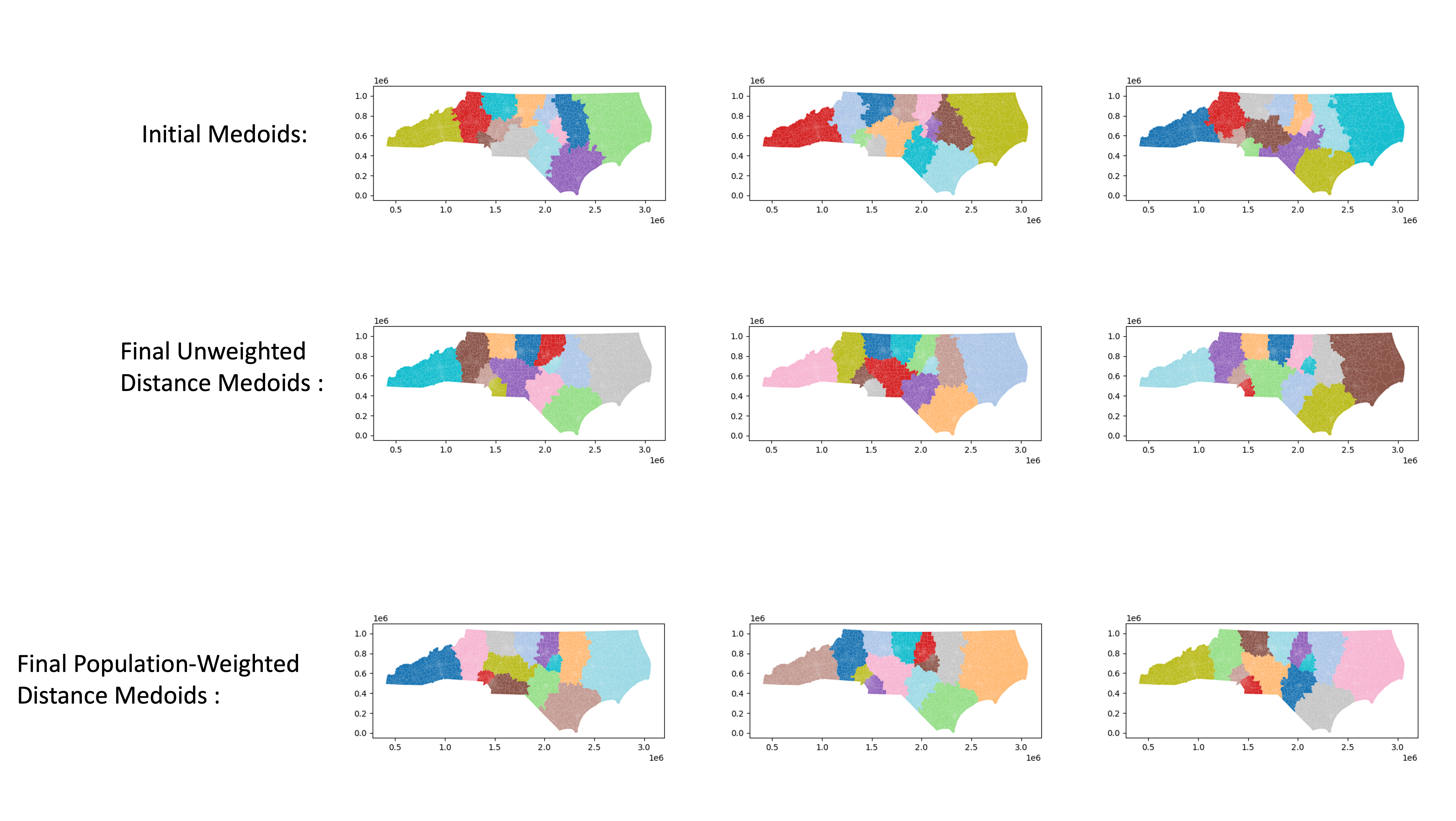
Figure 10: NC Medoids. (Top Row): Initial Medoids, (Middle Row): Final Unweighted Distance Medoids, and (Bottom Row): Final Population-Weighted Distance Medoids. Each column is for a specific seed and its associated centroid.

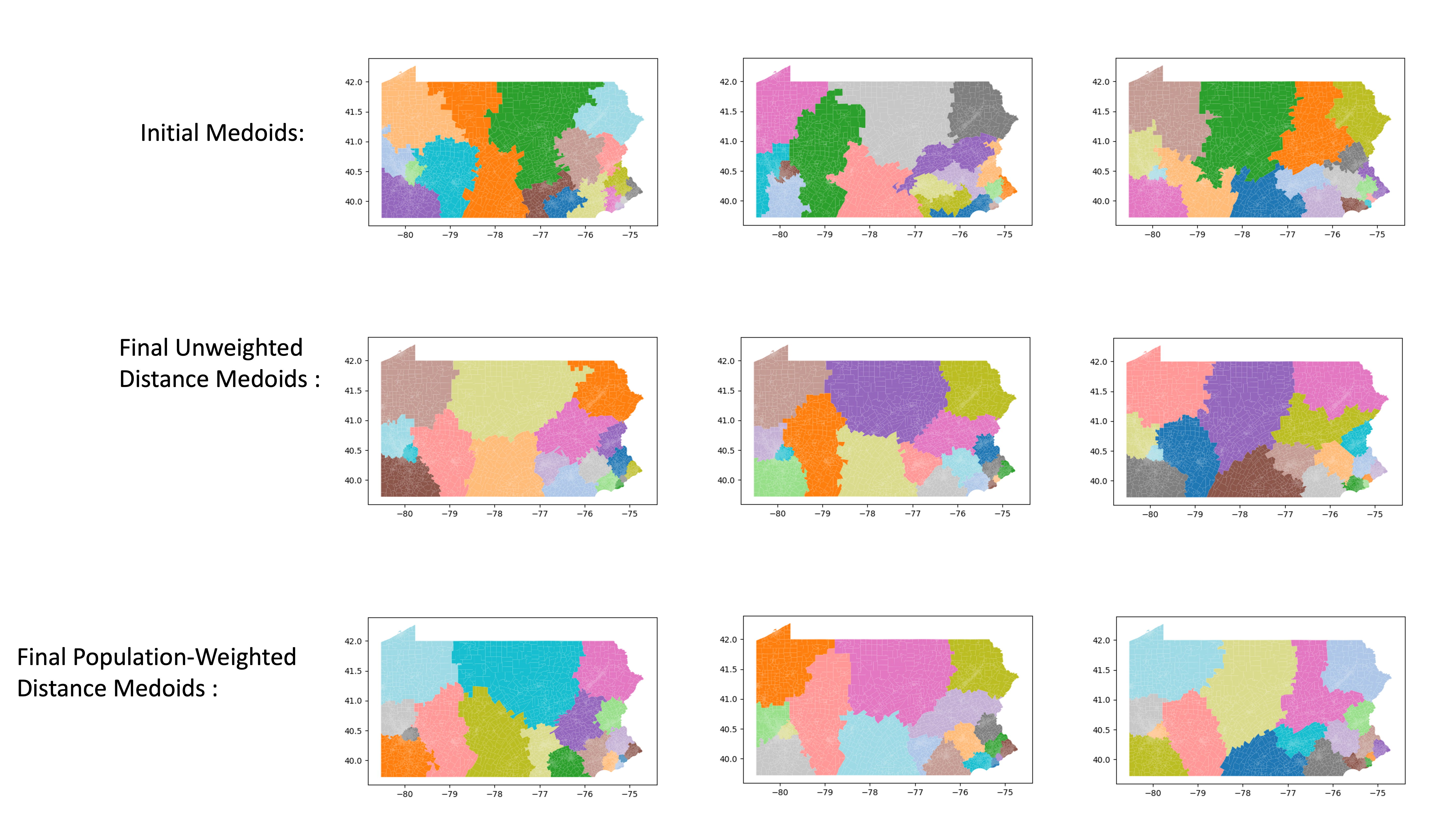
Figure 11: PA Medoids. (Top Row): Initial Medoids, (Middle Row): Final Unweighted Distance Medoids, and (Bottom Row): Final Population-Weighted Distance Medoids. Each column is for a specific seed and its associated centroid.

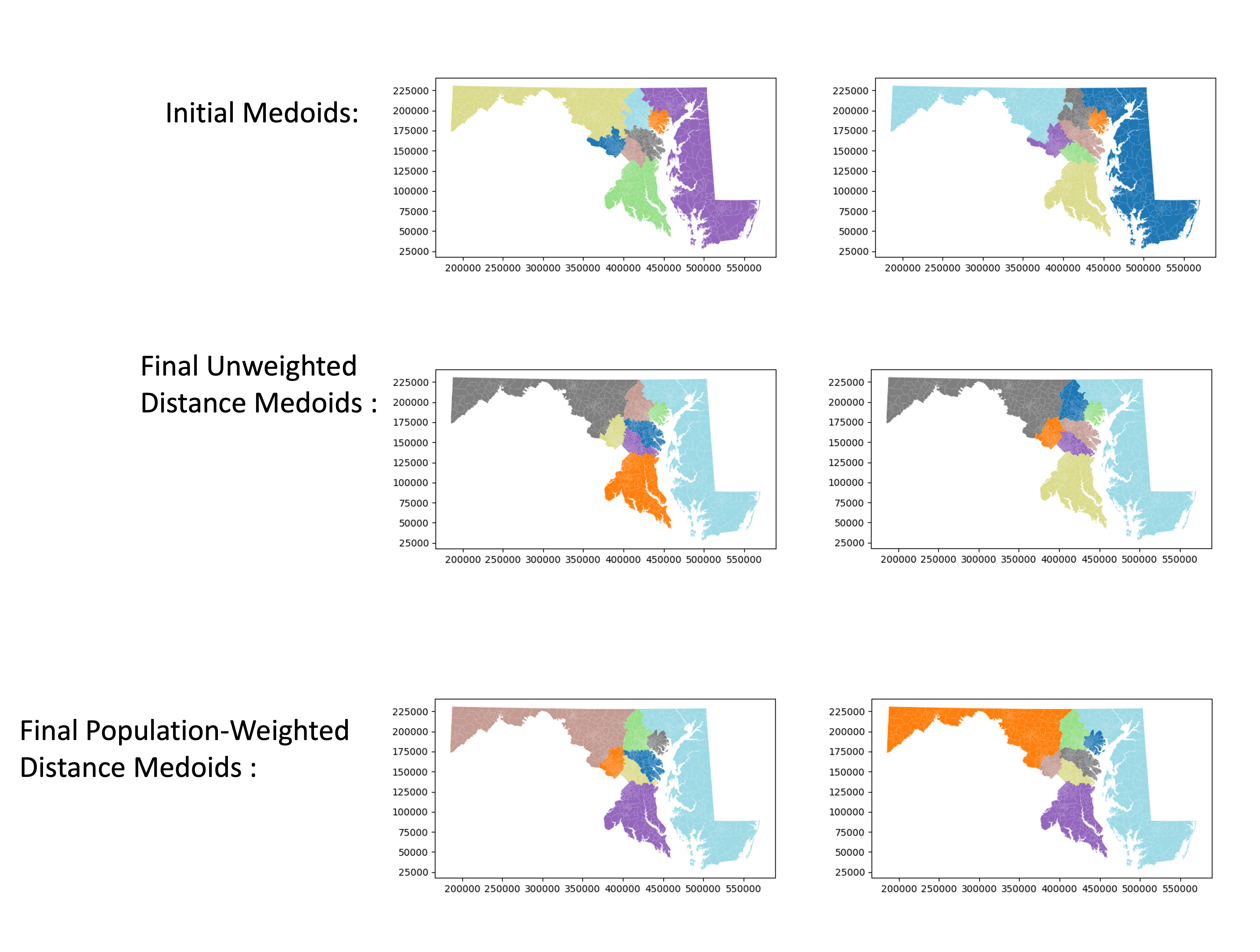
Figure 12: MD Medoids. (Top Row): Initial Medoids, (Middle Row): Final Unweighted Distance Medoids, and (Bottom Row): Final Population-Weighted Distance Medoids. Each column is for a specific seed and its associated centroid.

C.3.2 Relative Error $\operatorname{\textbf{RE}}(.,.)$ between the Final Medoids

Since we have three final medoids for each state and distance measure, we report the maximum relative error value that can be obtained using any pair of maps. Table 6 shows the maximum relative error percentage value, clearly the largest relative error value is at most around $3.87\%$.

Table 6: Maximum Relative Error $\operatorname{\textbf{RE}}$ between final medoids for each state and distance measure

STATE	Distance Measure	Max $\operatorname{\textbf{RE}}(.,)$ Percentage Value Over Final Medoid Pair
NC	Unweighted	$0.1701$
NC	Population-Weighted	$3.2506$
PA	Unweighted	$1.3482$
PA	Population-Weighted	$3.5210$
MD	Unweighted	$3.6167$
MD	Population-Weighted	$3.8749$

C.3.3 Election Histograms and Medoid Election Results

Here we show the election histogram for each state using votes for a specific election. First, note according to the distribution of votes in each district the number of seats won by a specific party can be calculated. Since we have two-party results, we show only the seats for one party (Democratic party). Finding election histograms using sampling methods is well-established DeFord et al., (2019); Herschlag et al., (2020) therefore we show only one histogram for each state, see Figures 13,14, and 15. We note that the election histograms are the same independent of the choice of seed (as expected). Further, election histograms are not related to a centroid or a chosen distance measure. For each state and distance measure, we record the number of seats for the final medoid maps as shown in the election tables below. In general, medoid maps lead to election results that have high probability, the outcome with the highest probability or close to it. Moreover, we find that the election outcomes of different medoids can significantly overlap.

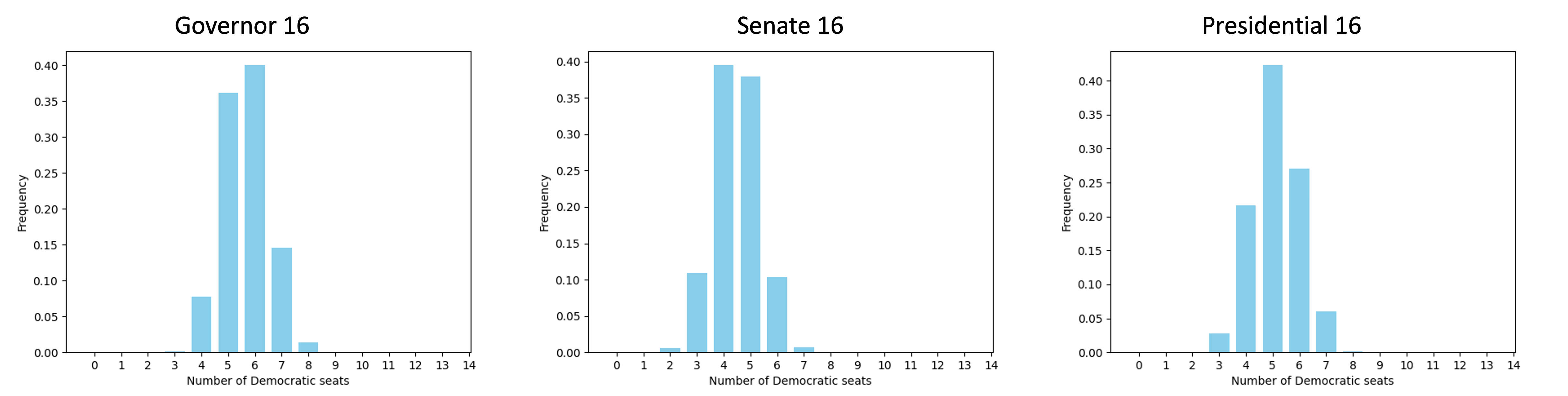
Figure 13: NC Election Histograms.

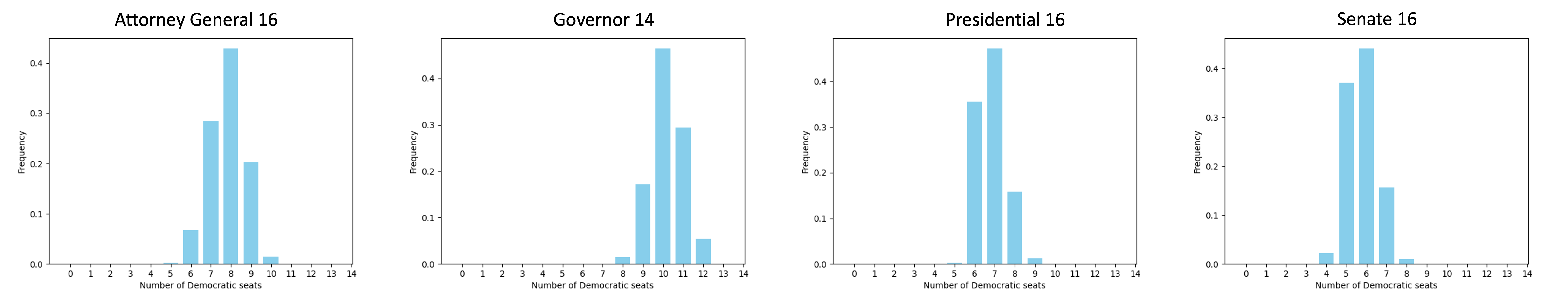
Figure 14: PA Election Histograms.

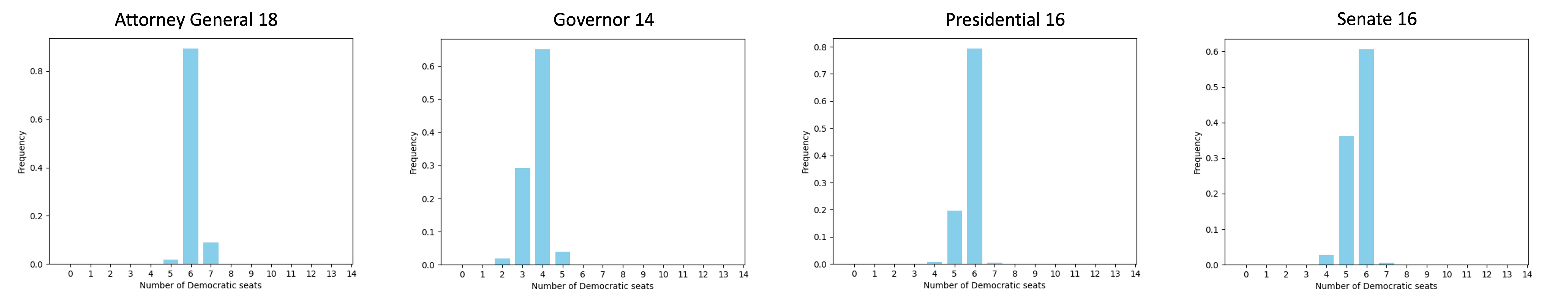
Figure 15: MD Election Histograms.

Table 7: Election results for the unweighted NC medoids.

Starting Seed	Governor 16	Senate 16	Presidential 16
Seed 1	5	4	5
Seed 2	6	4	5
Seed 3	6	4	5

Table 8: Election results for the weighted NC medoids.

Starting Seed	Governor 16	Senate 16	Presidential 16
Seed 1	5	4	4
Seed 2	6	4	5
Seed 3	6	4	6

Table 9: Election results for the unweighted PA medoids.

Starting Seed	Attorney General 16	Governor 14	Presidential 16	Senate 16
Seed 1	8	10	6	6
Seed 2	8	9	7	6
Seed 3	7	10	6	6

Table 10: Election results for the weighted PA medoids.

Starting Seed	Attorney General 16	Governor 14	Presidential 16	Senate 16
Seed 1	8	9	7	5
Seed 2	8	9	7	6
Seed 3	8	10	6	6

Table 11: Election results for the unweighted MD medoids.

Starting Seed	Attorney General 18	Governor 14	Presidential 16	Senate 16
Seed 1	6	4	6	5
Seed 2	6	4	6	6

Table 12: Election results for the weighted MD medoids.

Starting Seed	Attorney General 18	Governor 14	Presidential 16	Senate 16
Seed 1	6	4	6	5
Seed 2	6	4	6	6

References

- Abrishami et al., (2020) Abrishami, T., Guillen, N., Rule, P., Schutzman, Z., Solomon, J., Weighill, T., and Wu, S. (2020). Geometry of graph partitions via optimal transport. SIAM Journal on Scientific Computing, 42(5):A3340–A3366.
- Alexeev and Mixon, (2018) Alexeev, B. and Mixon, D. G. (2018). An impossibility theorem for gerrymandering. The American Mathematical Monthly, 125:878–884.
- Ashtiani et al., (2016) Ashtiani, H., Kushagra, S., and Ben-David, S. (2016). Clustering with same-cluster queries. Advances in neural information processing systems, 29.
- Brandt et al., (2016) Brandt, F., Conitzer, V., Endriss, U., Lang, J., and Procaccia, A. D. (2016). Handbook of computational social choice. Cambridge University Press.
- Brubach et al., (2020) Brubach, B., Srinivasan, A., and Zhao, S. (2020). Meddling metrics: the effects of measuring and constraining partisan gerrymandering on voter incentives. In Proceedings of the 21st ACM Conference on Economics and Computation, pages 815–833.
- Bycoffe et al., (2018) Bycoffe, A., Koeze, E., Wasserman, D., and Wolfe, J. (2018). The Atlas Of Redistricting. https://projects.fivethirtyeight.com/redistricting-maps/. [Online; published 25-January-2018; accessed 15-August-2019].
- Chen, (2021) Chen, M. (2021). Tufts research lab aids states with redistricting process. The Tufts Daily.
- Chhabra et al., (2020) Chhabra, A., Roy, A., and Mohapatra, P. (2020). Suspicion-free adversarial attacks on clustering algorithms. In Proceedings of the AAAI Conference on Artificial Intelligence, volume 34, pages 3625–3632.
- Chikina et al., (2017) Chikina, M., Frieze, A., and Pegden, W. (2017). Assessing significance in a markov chain without mixing. Proceedings of the National Academy of Sciences, 114(11):2860–2864.
- Cho, (2019) Cho, W. K. T. (2019). Technology-enabled coin flips for judging partisan gerrymandering. Southern California law review, 93.
- Cinà et al., (2022) Cinà, A. E., Torcinovich, A., and Pelillo, M. (2022). A black-box adversarial attack for poisoning clustering. Pattern Recognition, 122:108306.
- Cohen-Addad et al., (2018) Cohen-Addad, V., Klein, P. N., and Young, N. E. (2018). Balanced centroidal power diagrams for redistricting. In Proceedings of the 26th ACM SIGSPATIAL International Conference on Advances in Geographic Information Systems, pages 389–396.
- Commission, (2021) Commission, M. C. R. (2021). Redistricting Map Submission Process. https://redistricting.maryland.gov/Pages/plan-proposals.aspx. [Online; accessed 20-October-2021].
- DeFord and Duchin, (2019) DeFord, D. and Duchin, M. (2019). Redistricting reform in virginia: Districting criteria in context. Virginia Policy Review, 12(2):120–146.
- DeFord et al., (2019) DeFord, D., Duchin, M., and Solomon, J. (2019). Recombination: A family of markov chains for redistricting. arXiv preprint arXiv:1911.05725.
- Fifield et al., (2015) Fifield, B., Higgins, M., Imai, K., and Tarr, A. (2015). A new automated redistricting simulator using markov chain monte carlo. Work. Pap., Princeton Univ., Princeton, NJ.
- Goldschmidt and Hochbaum, (1994) Goldschmidt, O. and Hochbaum, D. S. (1994). A polynomial algorithm for the k-cut problem for fixed k. Mathematics of operations research, 19(1):24–37.
- He et al., (2003) He, Z., Xu, X., and Deng, S. (2003). Discovering cluster-based local outliers. Pattern recognition letters, 24(9-10):1641–1650.
- Herschlag et al., (2020) Herschlag, G., Kang, H. S., Luo, J., Graves, C. V., Bangia, S., Ravier, R., and Mattingly, J. C. (2020). Quantifying gerrymandering in north carolina. Statistics and Public Policy, 7(1):30–38.
- Hettle et al., (2021) Hettle, C., Zhu, S., Gupta, S., and Xie, Y. (2021). Balanced districting on grid graphs with provable compactness and contiguity. arXiv preprint arXiv:2102.05028.
- Kemeny, (1959) Kemeny, J. G. (1959). Mathematics without numbers. Daedalus, 88(4):577–591.
- Kendall, (1938) Kendall, M. G. (1938). A new measure of rank correlation. Biometrika, 30(1/2):81–93.
- Knox and Ng, (1998) Knox, E. M. and Ng, R. T. (1998). Algorithms for mining distancebased outliers in large datasets. In Proceedings of the international conference on very large data bases, pages 392–403. Citeseer.
- Liu et al., (2016) Liu, Y. Y., Cho, W. K. T., and Wang, S. (2016). Pear: a massively parallel evolutionary computation approach for political redistricting optimization and analysis. Swarm and Evolutionary Computation, 30:78 – 92.
- LWV vs Commonwealth of Pennsylvania, (2018) LWV vs Commonwealth of Pennsylvania (No. 159 MM (2018)).
- Mattingly and Vaughn, (2014) Mattingly, J. C. and Vaughn, C. (2014). Redistricting and the will of the people. arXiv preprint arXiv:1410.8796.
- Newling and Fleuret, (2017) Newling, J. and Fleuret, F. (2017). A sub-quadratic exact medoid algorithm. In Artificial Intelligence and Statistics, pages 185–193. PMLR.
- Pegden et al., (2017) Pegden, W., Procaccia, A. D., and Yu, D. (2017). A partisan districting protocol with provably nonpartisan outcomes. arXiv preprint arXiv:1710.08781.
- Polsby and Popper, (1991) Polsby, D. D. and Popper, R. D. (1991). The third criterion: Compactness as a procedural safeguard against partisan gerrymandering. Yale Law & Policy Review, 9(2):301–353.
- Rucho v. Common Cause, (2019) Rucho v. Common Cause (No. 18-422, 588 U.S. ___ (2019)).
- Ryan and Smith, (2022) Ryan, I. and Smith, W. D. (2022). Splitline districtings of all 50 states + DC + PR. https://rangevoting.org/SplitLR.html. [Online; accessed 15-August-2019].
- Saran and Vazirani, (1995) Saran, H. and Vazirani, V. V. (1995). Finding k cuts within twice the optimal. SIAM Journal on Computing, 24(1):101–108.
- Validi and Buchanan, (2022) Validi, H. and Buchanan, A. (2022). Political districting to minimize cut edges. Mathematical Programming Computation, pages 1–50.
- Vieth v. Jubelirer, (2004) Vieth v. Jubelirer (No. 02-1580, 541 U.S. 267 (2004)).
- Wu et al., (2015) Wu, L. C., Dou, J. X., Sleator, D., Frieze, A., and Miller, D. (2015). Impartial redistricting: A markov chain approach. arXiv preprint arXiv:1510.03247.
- Zubrzycki, (1972) Zubrzycki, S. (1972). Lectures in probability theory and mathematical statistics, volume 38. Elsevier Publishing Company.