An Instance Space Analysis of Constrained Multi-Objective Optimization Problems

Abstract

Multi-objective optimization problems with constraints (CMOPs) are generally considered more challenging than those without constraints. This in part can be attributed to the creation of infeasible regions generated by the constraint functions, and/or the interaction between constraints and objectives. In this paper, we explore the relationship between constrained multi-objective evolutionary algorithms (CMOEAs) performance and CMOP instances characteristics using Instance Space Analysis (ISA). To do this, we extend recent work focused on the use of Landscape Analysis features to characterise CMOP. Specifically, we scrutinise the multi-objective landscape and introduce new features to describe the multi-objective-violation landscape, formed by the interaction between constraint violation and multi-objective fitness. Detailed evaluation of problem-algorithm footprints spanning six CMOP benchmark suites and fifteen CMOEAs, illustrates that ISA can effectively capture the strength and weakness of the CMOEAs. We conclude that two key characteristics, the isolation of non-dominate set and the correlation between constraints and objectives evolvability, have the greatest impact on algorithm performance. However, the current benchmarks problems do not provide enough diversity to fully reveal the efficacy of CMOEAs evaluated.

I Introduction

Constrained multi-objective optimization problems (CMOPs) involve searching for the best trade-off between multiple conflicting objectives subject to one or more constraints. Many real-world optimization problems match this description, in areas as diverse as mechanical design, chemical engineering, and power system optimization [1]. Generally, a CMOP is more challenging than its unconstrained counterpart due to the addition of one or more constraint functions, and the resulting interactions between the constraints and the objectives  [2]. Constraints may change the shape and location of the Pareto front $\left(PF\right)$, often creating only small feasible regions, resulting in additional difficulties when attempting to generate a diverse set of solutions on the $PF$. Consequently, several constrained multi-objective evolutionary algorithms (CMOEAs) have been introduced to specifically tackle CMOPs [3]. However, as per many other problem domains, practice has shown that no single algorithm outperforms all other algorithms across all problem instances [4, 1]. Each algorithm has its strengths and weaknesses, and it is hard to choose the best one for solving a particular instance. Therefore, it is necessary to understand when an algorithm is suitable or not, i.e., when it performs well and when it fails, which requires an understanding of the characteristics of the instances being solved, e.g. multi-modality and variable scaling, and what distinguish the instances from each other [5].

In this paper, we explore the relationship between algorithm performance and CMOP instances characteristics using Instance Space Analysis (ISA). Proposed by Smith-Miles et al., [6], ISA is a methodology for assessing the difficulty of a set of problem instances for a group of algorithms. Figure 1 illustrates ISA’s framework, which uses a meta-data set consisting of features that characterize a set of instances, and performance measures of a group of algorithms on those instances. Then, by selecting a subset of uncorrelated features that are predictive of algorithm performance, and using a tailored dimensionality reduction method, the meta-data is projected into a 2-dimensional plane called the instance space. In it, each instance is represented as a point, allowing for the visualization of the similarities and differences between instances, in terms of characteristics and algorithm performance. An examination of the generated instance space can then be used to identify regions of good performance, called footprints, where an algorithm is expected to perform well and why.

ISA has been employed successfully on related problem domains. For example, Yap et al., [7] performed an ISA of combinatorial multi-objective optimization problems (MOPs), discovering that MOEA/D is preferred, not only when the number of objectives increased, but also when the degree of conflict between objectives decreased. Similarly, Muñoz and Smith-Miles [8] analyzed the space of continuous single-objective optimization problems, identifying that multi-modal instances with adequate global structure are hard to solve by most studied algorithms with exception to BIPOP-CMA-ES. In both works, Landscape Analysis features [9] were employed to characterize a problem instance. Therefore, a necessary first step when applying ISA for CMOP will be to identify and calculate appropriate, informative Landscape Analysis features.

Recent work have proposed Landscape Analysis features for characterizing MOPs. Kerschke et al., [10] studied the notion of multimodality in MOPs and provided a set of features to quantify it, whilst Liefooghe et al., [11] extended previous works in the combinatorial MOPs domain to characterize continuous MOPs, focusing on multimodality, evolvability, and ruggedness. Unfortunately, it is not a straight forward task to identify Landscape Analysis features for CMOP. The features described above can be used in the CMOP domain to help characterize the objective space. However, features associated with the constraints violation, and features representing the interaction between objectives and constraints are required.

There have been only a few attempts to characterize constrained optimization problems. For example, for single-objective problems Malan et al., [12] defined the concept of a Violation landscape, proposing four features to characterize the feasible and constrained spaces. In other work, Poursoltan and Neumann [13] introduced a biased sampling technique to quantify the ruggedness of a constrained optimization problems. Picard and Schiffmann [14] focussing on CMOPs, adopted two features from [12], and extended another so that it could be used to measure ‘disjointedness’ of the feasible regions. They also proposed two features to quantify the relationship between objectives and constraints. Vodopija et al., [15] were the first to introduce violation multimodality in CMOPs, proposing a set of features to characterize violation multimodality, smoothness, and the correlation between the objectives and constraints. They then used those features to compare the characteristics of eight benchmark problem suites against a real-world suite. This work did provide important insights, however, the approach was limited to the Violation landscape and did not capture important aspects that need to be quantified, such as the relationship between the constrained and unconstrained PF, or the ruggedness and evolvability of the multi-objective-violation landscape.

To construct the first ISA for continuous CMOP, we introduce the multi-objective-violation landscape, formed by the interaction between constraint violation and multi-objective fitness. This required the introduction of 12 new features and modification of 22 existing features to quantify the characteristics of the Violation landscape and multi-objective-violation landscape. The meta-data set was then generated for the instance space by processing the features for six CMOP benchmark suites and the performance of 15 CMOEAs.

Comprehensive analysis of the generated footprints illustrates that ISA can effectively capture the strength and weakness of the CMOEAs. A key observation is that there are two characteristics in particular that affect the performance of most CMOEAs – the isolation of the non-dominate set and the correlation between constraints and objectives. However, the performance of each CMOEA is affected by a different set of features. Importantly, the footprints provided strong supporting visual evidence as to which characteristics are necessary if any new proposed benchmarks are to significantly challenge CMOEAs.

The remainder of the paper is organized as follows: Section II presents the ISA methodology and its components, which are the problem include CMOPs definition, benchmark suites, landscape features, CMOEAs, and performance metric. Section III describes the experimental setup. The results are presented and discussed in section IV. Finally, section V concludes the paper.

Figure 1: Summary of the Instance Space Analysis framework [16].

II Instance Space Analysis

Instance Space Analysis (ISA) traces its foundations to Rice’s framework for solving the Algorithm Selection Problem [17], which suggests the construction of a selection mapping between measurable features of a problem and a set of suitable algorithms; and Wolpert and Macready’s No-Free Lunch theorems [18], which state that an algorithm is unlikely to outperform all other algorithms on all possible instances. Figure 1 illustrates ISA’s framework, which has at its core six component spaces or sets [16]: (a) the problem space, $\mathcal{P}$, containing all the relevant instances of a problem in an application domain; (b) a subset of instances, $\mathbf{I}$, for which we have meta-data from computational experiments; (c) the feature space, $\mathcal{F}$, which are used to characterize the mathematical and statistical properties of the instances; (d) the algorithm space, $\mathcal{A}$, representing the set of algorithms available to solve all instances in $\mathbf{I}$; (e) the performance space, $\mathcal{Y}$, composed of a measure of the computational effort to obtain a satisfactory solution; and (f) the instance space, a 2-dimensional visualization that aids on the observation of trends in hardness for different algorithms, and facilitates insights into the distribution of existing instances.

This section describes the details for each one of the spaces in the ISA framework, tailored specifically for CMOPs. We start with $\mathcal{P}$ by formally defining a CMOP. Then, we present $\mathbf{I}$, drawn from six commonly used benchmark suites. Next, we describe $\mathcal{F}$, where we introduce the multi-objective-violation Landscape, as well as a set of new features for characterizing CMOPs. We follow by describing $\mathcal{A}$, by briefly presenting the 15 algorithms under test, and $\mathcal{Y}$ by formally defining the hyper-volume, our performance metric.

II-A Problem Space

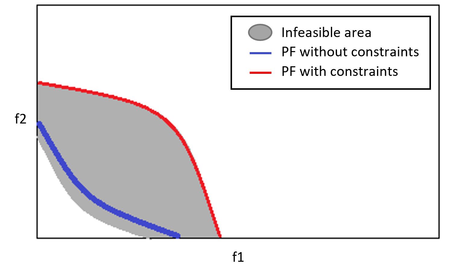
(a)

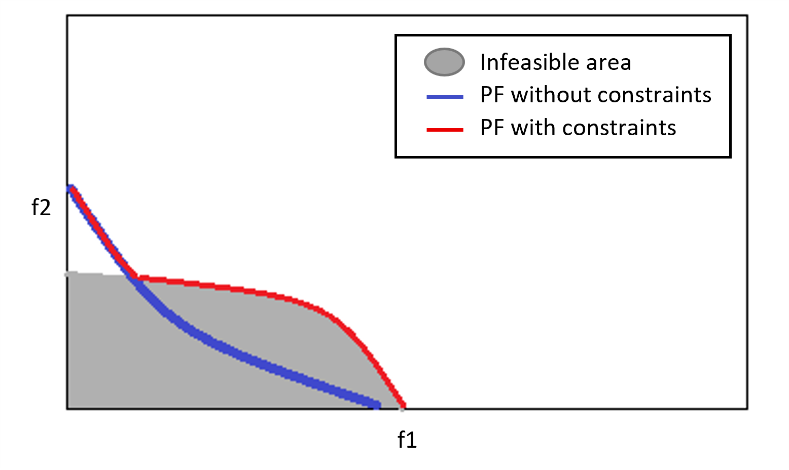
(b)

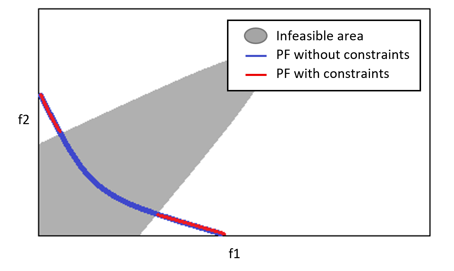
(c)

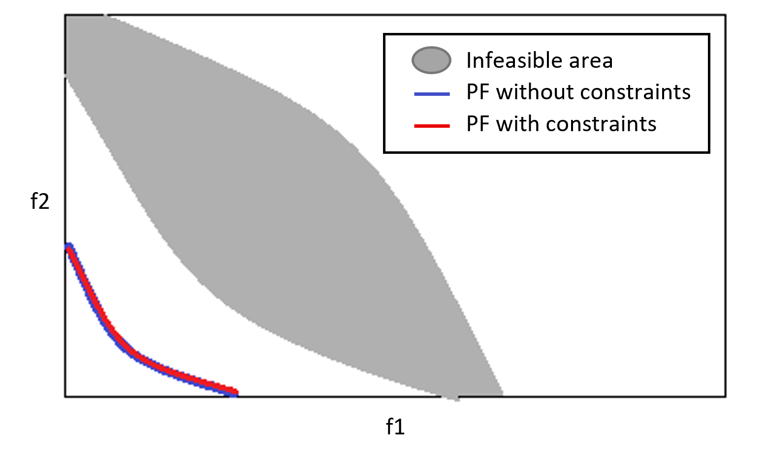
(d)

Figure 2: Effect of constraints on the $PF$: LABEL:sub@fig:CPF1 The $UPF$ is no longer feasible, and the true $PF$ lies completely on bounds of the feasible region; LABEL:sub@fig:CPF2 part of the $UPF$ is no longer feasible, and parts of the true $PF$ lies on bounds of the feasible region; LABEL:sub@fig:CPF3 the true $PF$ is only a proportion of the $UPF$; and LABEL:sub@fig:CPF4 an infeasible region blocks the way toward the $PF$.

A CMOP can be defined as finding a vector of decision variables that optimizes a set of objective functions and satisfies a set of restrictions. Without loosing generality, we assume minimization. CMOP can be mathematically defined as follows:

$$\left.\begin{array}[]{rll}\min&f_{m}(x),&m=1,2,\ldots,M\\ \text{s.t.}&g_{j}(x)\geq 0,&j=1,2,\ldots,J\\ &h_{k}(x)=0,&k=1,2,\ldots,K\\ &x_{i}^{(L)}\leq x_{i}\leq x_{i}^{(U)},&i=1,2,\ldots,n\end{array}\right\}$$ (1)

where a solution $x\in R^{n}$ is a vector of $n$ decision variables, $f(x)$ is a vector of $M$ objectives to be optimized, $g(x)$ is set of $J$ inequality constraints, while $h(x)$ is set of $K$ equality constraints, and $x_{i}^{(L)}$ and $x_{i}^{(U)}$ represent respectively the lower and upper bounds of a decision variable $x_{i}$. The constraints violation of a solution $x$ can be calculated by the following equation:

$$CV\left({x}\right)=\sqrt{\sum_{j=1}^{J}G_{j}\left({x}\right)^{2}+\sum_{k=1}^{K}H_{k}\left({x}\right)^{2}}$$ (2)

where

$$G_{j}\left({x}\right)=\max\left(0,g_{j}\left({x}\right)\right)$$ (3)

and

$$H_{k}\left({x}\right)=\max\left(0,\left|h_{k}\left({x}\right)\right|-\epsilon\right)$$ (4)

where $\epsilon$ is a small value $\left({10}^{-4}\right)$ to relax the equality constraints. A solution to the problem is feasible when it satisfies the sets of constraints, otherwise the solution is infeasible.

A solution $x\in R^{n}$ is said to be Pareto optimal if there is no other feasible solution $y\in R^{n}$ such that $f(y)\prec f(x)$, where $\prec$ indicates the Pareto dominance relation. That is, a feasible solution $x$ dominates a feasible solution $y$ if and only if no objective value of $f(x)$ is greater than $f(y)$ and at least one objective value is smaller. Because of the conflicting nature of the multiple objectives, optimizing one objective function may lead to a degradation in another. Therefore, a single optimal solution may no longer be found, but instead a set of trade-off solutions, the so-called non-dominated solutions or Pareto optimal set ($PS$). Those set of solutions represent the Pareto optimal front ($PF$) in the objective space.

When solving a MOP, an algorithm aims to find an estimated front, $\widetilde{PF}$, that has converged, i.e., is as close as possible to the $PF$, and is diverse, i.e., represents the whole $PF$. In CMOPs, the feasibility of the solution(s) must also be considered. The true, constrained, $PF$ of a CMOP can be determined by the unconstrained $PF$ ($UPF$) and bounds of the feasible regions in the objective space. Having a low proportion of feasible regions typically adds to the challenge/difficulty of the search process. In addition, the infeasible regions may affect the shape of the $PF$ or split it into many segments, which may impact the algorithm’s ability to provide diversity in its solutions. That is, the infeasible regions may block the trajectory of the search towards $PF$, limiting convergence [2]. Figure 2 illustrates examples of difficulties caused by constraints.

II-B Subset of instances

Test problems should cover as many characteristics of real-world problems as possible, if an evaluation of the performance of the optimization algorithm is to provide useful insights before solving an expensive real-world problem. Several CMOP benchmarks have been designed with this goal in mind. Ma and Wang [19] proposed a classification of CMOPs depending on the relationship between $UPF$ and the $PF$:

Type I

the $PF$ is same as the $UPF$.

Type II

the $PF$ is part of the $UPF$.

Type III

the $PF$ contains all or part of the $UPF$ and solutions on the boundary of the feasible region.

Type IV

the $PF$ is completely located on the boundary of the feasible region.

We have used six benchmark suites in this work: CF [20], C-DTLZ [21], DC-DTLZ [22], LIR-CMOP [23], DAS-CMOP [2], and MWs [19]. These suites have a wide range of characteristics, which are summarized in Table I.

TABLE I: Characteristics of the benchmarks employed in this study. All of them have a scalable number of decision variables. Type describes the relationship between $UPF$ and $PF$, $M$ is the number of objectives, $CF$ is the number of constraints, $UPF$ and $PF$ columns define their shape, and the size and connectivity of the feasible region is given in the last column. S is short for scalable, C for Controllable, Disconn for Disconnected, Conn for Connected, L for Large, and S for Small.

Problem	Type	M	CF	UPF	PF	Feasible Region
CF1	II	2	1	Linear	Disconn	L/Conn
CF2	II	2	1	Convex	Disconn	L/Conn
CF3	II	2	1	Concave	Disconn	L/Conn
CF4	III	2	1	Linear	Linear	L/Conn
CF5	III	2	1	Linear	Linear	L/Conn
CF6	III	2	1	Convex	Mixed	L/Conn
CF7	III	2	1	Convex	Mixed	L/Conn
CF8	II	3	1	Concave	Disconn	L/Conn
CF9	II	3	1	Concave	Disconn	L/Conn
CF10	II	3	1	Concave	Disconn	L/Conn
C1-DTLZ1	I	S	1	Linear	Linear	S/Conn
C2-DTLZ2	II	S	1	Concave	Concave	S/Disconn
C1-DTLZ3	I	S	1	Concave	Concave	L/Disconn
C3-DTLZ4	IV	S	M	Concave	Concave	L/Conn
DC1-DTLZ1	II	S	1	Linear	Disconn	C/Disconn
DC1-DTLZ3	II	S	1	Concave	Disconn	C/Disconn
DC2-DTLZ1	I	S	2	Linear	Linear	S/Disconn
DC2-DTLZ3	I	S	2	Concave	Concave	S/Disconn
DC3-DTLZ1	II	S	M	Linear	Disconn	C/Disconn
DC3-DTLZ3	II	S	M	Concave	Disconn	C/Disconn
DAS-CMOP1	C	2	11	Concave	Disconn	C/C
DAS-CMOP2	C	2	11	Mixed	Mixed	C/C
DAS-CMOP3	C	2	11	Disconn	Disconn	C/C
DAS-CMOP4	C	2	11	Concave	Disconn	C/C
DAS-CMOP5	C	2	11	Mixed	Mixed	C/C
DAS-CMOP6	C	2	11	Disconn	Disconn	C/C
DAS-CMOP7	C	3	7	Linear	Disconn	C/C
DAS-CMOP8	C	3	7	Concave	Disconn	C/C
DAS-CMOP9	C	3	7	Concave	Disconn	C/C
LIR-CMOP1	IV	2	2	Concave	Concave	S/Conn
LIR-CMOP2	IV	2	2	Convex	Convex	S/Conn
LIR-CMOP3	IV	2	3	Concave	Disconn	S/Disconn
LIR-CMOP4	IV	2	3	Convex	Disconn	S/Disconn
LIR-CMOP5	I	2	2	Convex	Convex	S/Disconn
LIR-CMOP6	I	2	2	Concave	Concave	S/Disconn
LIR-CMOP7	IV	2	3	Convex	Concave	S/Disconn
LIR-CMOP8	IV	2	3	Concave	Concave	S/Disconn
LIR-CMOP9	II	2	2	Concave	Disconn	S/Disconn
LIR-CMOP10	II	2	2	Convex	Disconn	S/Disconn
LIR-CMOP11	III	2	2	Convex	Disconn	S/Disconn
LIR-CMOP12	III	2	2	Concave	Disconn	S/Disconn
LIR-CMOP13	I	3	2	Mixed	Mixed	S/Disconn
LIR-CMOP14	II	3	3	Mixed	Mixed	S/Disconn
MW1	II	2	1	Linear	Disconn	S/Disconn
MW2	I	2	1	Linear	Linear	S/Disconn
MW3	III	2	2	Linear	Mixed	S/Conn
MW4	I	S	1	Linear	Linear	S/Conn
MW5	II	2	3	Concave	Disconn	S/Conn
MW6	II	2	1	Concave	Disconn	S/Disconn
MW7	III	2	2	Concave	Disconn	S/Conn
MW8	II	S	1	Concave	Disconn	S/Disconn
MW9	IV	2	1	Convex	Concave	S/Conn
MW10	III	2	3	Concave	Disconn	S/Disconn
MW11	IV	2	4	Concave	Disconn	S/Disconn
MW12	IV	2	2	Mixed	Mixed	S/Disconn
MW13	III	2	2	Disconn	Disconn	S/Disconn
MW14	I	S	1	Disconn	Disconn	S/Conn

II-C Feature Space

Landscape Analysis are methods used to quantify the characteristics of a problem’s landscape, which is described as a surface in the search space that defines a certain aspect of the problem, such as fitness, for each potential solution [5]. Stadler [24] defined a general form of the fitness landscape for a problem as the triplet $\left(X,N,f\right)$, where $X$ is a set of potential solutions, $f$ is a fitness function, and $N$ is a notion of neighborhood relation. The Euclidean distance is usually used in continuous optimization to quantify solutions relations.

Constrained multi-objective optimization involves multiple fitness and constraint functions; hence, Stadler’s definition of fitness landscape cannot be directly applied in this work. Verel et al., [25] defined the multi-Objective landscape, and Malan et al., [12] introduced the violation landscape. However, these two landscapes treat constraints and objectives independently. Therefore, they do not capture the interaction between them, which is essential for CMOPs. Consequently, we introduce the concept of the multi-objective-violation landscape in II-C3. Also, we propose a set of local structured-based landscape features collected by random walks, and global unstructured-based landscape features approximated by random samples [26]. In the next subsections, we present the three landscapes and their features in detail.

TABLE II: The features used to characterize the Multi-Objectives Landscape of CMOP.

Type	Feature	Description	Source	Focus
Global	upo_n	Proportion of unconstrained PO solutions	[27]	Set-Cardinality
	uhv	Hypervolume-value of the unconstrained PF	[28]	Set-Distribution
	corr_obj	correlation between objective values	[29]	evolvability
	mean_f	Average of unconstrained ranks	[11]	y-distribution
	std_f	Standard deviation of unconstrained ranks	[5]	y-distribution
	max_f	Maximum of unconstrained ranks	[5]	y-distribution
	skew_f	Skewness of unconstrained ranks	[5]	y-distribution
	kurt_f	Kurtosis of unconstrained ranks	[5]	y-distribution
	kurt_avg	Average of objectives kurtosis	[5]	y-distribution
	kurt_min	Minimum of objectives kurtosis	[5]	y-distribution
	kurt_max	Maximum of objectives kurtosis	[5]	y-distribution
	kurt_rnge	Range of objectives kurtosis	[5]	y-distribution
	skew_avg	Average of objectives skewness	[5]	y-distribution
	skew_min	Minimum of objectives skewness	[5]	y-distribution
	skew_max	Maximum of objectives skewness	[5]	y-distribution
	skew_rnge	Range of objectives skewness	[5]	y-distribution
	f_mdl_r2	Adjusted coefficient of determination of a linear regression model for varibles and unconstrained ranks	[5]	variable scaling
	f_range_coeff	Difference between maximum and minimum of the absolute value of the linear model coefficients	[5]	variable scaling
Random Walk	dist_f_avg_rws	Average distance from neighbours in the objective space	[11]	evolvability
	dist_f_r1_rws	First autocorrelation coefficient of dist_f_avg_rws	[11]	ruggedness
	dist_f_dist_x_avg_rws	Ratio of dist_f_avg_rws to dist_x_avg_rws	[11]	evolvability
	dist_f_dist_x_avg_r1	First autocorrelation coefficient of dist_f_dist_x_avg_rws	[11]	ruggedness
	nuhv_avg_rws	Average unconstrained hypervolume-value of neighborhood’s solutions	[29]	evolvability
	nuhv_r1_rws	First autocorrelation coefficient of nuhv_avg_rws	[29]	ruggedness

TABLE III: The features used to characterize the Violation Landscape of CMOP. The proposed features marked as New, while the (*) indicates that the feature has been modified to characterize CMOP.

Type	Feature	Description	Source	Focus
Global	min_cv	Minimum of constraints violations	[5] *	y-distribution
	skew_cv	Skewness of constraints violations	[5] *	y-distribution
	kurt_cv	Kurtosis of constraints violations	[5] *	y-distribution
	cv_mdl_r2	Adjusted coefficient of determination of a linear regression model for varibles and violations	[5] *	variable scaling
	cv_range_coeff	Difference between maximum and minimum of the absolute value of the linear model coefficients	[5] *	variable scaling
	dist_c_corr	Violation-distance correlation	[30] *	deception
Random Walk	dist_c_avg_rws	Average distance from neighbours in the constraints space	[11] *	evolvability
	dist_c_r1_rws	first autocorrelation coefficient of dist_c_avg_rws	[11] *	ruggedness
	dist_c_dist_x_avg_rws	Ratio of dist_c_avg_rws to dist_x_avg_rws	[11] *	evolvability
	dist_c_dist_x_r1_rws	First autocorrelation coefficient of dist_c_dist_x_avg_rws	[11] *	ruggedness
	ncv_avg_rws	Average single solution’s violation-value	New	evolvability
	ncv_r1_rws	first autocorrelation coefficient of ncv_avg_rws	New	ruggedness
	nncv_avg_rws	Average neighborhood’s violation-value	New	evolvability
	nncv_r1_rws	first autocorrelation coefficient of nncv_avg_rws	New	ruggedness
	bncv_avg_rws	Average violation-value of neighborhood’s non-dominated solutions	New	evolvability
	bncv_r1_rws	first autocorrelation coefficient of bncv_avg_rws	New	ruggedness

TABLE IV: The features used to characterize the Multi-Objectives-Violation Landscape of CMOP. The proposed features marked as New, while the (*) indicates that the feature has been modified to characterize CMOP.

Type	Feature	Description	Source	Focus
Global	fsr	Feasibility ratio	[12]	Set-Cardinality
	po_n	Proportion of PO solutions	[27]	Set-Cardinality
	hv	Hypervolume-value of the PF	[28]	Set-Distribution
	cpo_upo_n	Proportion of PF to unconstrained PF	New	PF and UPF correlation
	hv_uhv_n	Proportion of HV to unconstrained HV	New	PF and UPF correlation
	GD_cpo_upo	distance between PF and unconstrained PF	New	PF and UPF correlation
	cover_cpo_upo	Proportion of unconstrained PF covered by PF	New	PF and UPF correlation
	corr_cobj_min	Minimum constraints and objectives correlation	[15]	evolvability
	corr_cobj_max	Maximum constraints and objectives correlation	[15]	evolvability
	corr_cf	Constraints and ranks correlation	[12] *	evolvability
	piz_ob_min	Minimum proportion of solutions in ideal zone per objectives	[12] *	Optima isolation
	piz_ob_max	Maximum proportion of solutions in ideal zone per objectives	[12] *	Optima isolation
	piz_f	Proportion of solutions in ideal zone	[12] *	Optima isolation
	ps_dist_max	Maximum distance across PS	[27]	PS connectivity
	ps_dist_mean	Average distance across PS	[31]	PS connectivity
	ps_dist_iqr_mean	Average difference between 75th and 25th percentiles of distances across PS	[31]	PS connectivity
	pf_dist_max	Maximum distance across PF	[32]	PF discontinuouty
	pf_dist_mean	Average distance across PF	[32]	PF discontinuouty
	pf_dist_iqr_mean	Average difference between 75th and 25th percentiles of distances across PF	[32]	PF discontinuouty
Random Walk	sup_avg_rws	Average proportion of neighbors dominating the current solution	[29]	evolvability
	sup_r1_rws	First autocorrelation coefficient of sup_avg_rws	[29]	ruggedness
	inf_avg_rws	Average proportion of neighbors dominated by the current solution	[29]	evolvability
	inf_r1_rws	First autocorrelation coefficient of inf_avg_rws	[29]	ruggedness
	inc_avg_rws	Average proportion of neighbors incomparable to the current solution	[29]	evolvability
	inc_r1_rws	First autocorrelation coefficient of inc_avg_rws	[29]	ruggedness
	lnd_avg_rws	Average proportion of locally non-dominated solutions in the neighborhood	[29]	evolvability
	lnd_r1_rws	First autocorrelation coefficient of lnd_avg_rws	[29]	ruggedness
	dist_x_avg_rws	Average distance from neighbours in the variable space	[11]	evolvability
	dist_x_r1_rws	First autocorrelation coefficient of dist_x_avg_rws	[11]	ruggedness
	dist_f_c_avg_rws	Average distance from neighbours in the objective-constraints space	[11] *	evolvability
	dist_f_c_r1_rws	First autocorrelation coefficient of dist_f_c_avg_rws	[11] *	ruggedness
	dist_f_c_dist_x_avg_rws	Ratio of dist_f_c_avg_rws to dist_x_avg_rws	[11] *	evolvability
	dist_f_c_dist_x_avg_r1	First autocorrelation coefficient of dist_f_c_dist_x_avg_rws	[11] *	ruggedness
	nhv_avg_rws	Average hypervolume-value of feasible neighborhood’s solutions	[29] *	evolvability
	nhv_r1_rws	First autocorrelation coefficient of nhv_avg_rws	[29] *	ruggedness
	bhv_avg_rws	Average hypervolume-value of neighborhood’s non-dominated solutions	[29] *	evolvability
	bhv_r1_rws	First autocorrelation coefficient of bhv_avg_rws	[29] *	ruggedness
	nfronts_avg_rws	Average number of ranks	New	evolvability
	nfronts_r1_rws	first autocorrelation coefficient of nfronts_avg_rws	New	ruggedness
	rfbx_rws_avg	Average ratio of feasible boundary crossings	[12]	Dispersion of the feasible regions

II-C1 Multi-Objective Landscapes

In multi-objective optimization, we are dealing with multiple fitness functions and set of optimal solutions. Therefore, Verel et al., [25] adjusted the elements of the fitness landscape to include multi-objective concepts by redefining $X$ as a set of solutions-sets, $f$ as multi-objective quality indicators, while $N$ depends on relations between solutions-sets. A set of features to characterize the multi-objective Landscape have been adopted from the literature and summarized in Table II.

II-C2 Violation Landscapes

For characterizing constrained optimization problems, Malan et al., [12] introduced the violation landscape, which uses the same elements as a fitness landscape, but replaces $f$ by a violation function. The violation function quantifies how much a solution violates the problem constraints. Here, we use the norm of constraints violation vector as calculated in Equation 2.

We propose six features to measure ruggedness and evolvability. From a random walk, we propose calculating average and first auto-correlation coefficient of the following: single solution’s violation-value (ncv), its neighborhood total violation-value (nncv), violation-value of neighborhood’s non-dominated solutions (bncv).

In addition, a set of features from the fitness landscape domain has been modified to quantify the characteristics of the violation landscape. To measure the distribution of the violation function, we used minimum, kurtosis, and skewness features. To measure variable scaling, we used features from a linear regression model fitted to decision variables and their violation-value (cv_mdl_r2 and cv_range_coeff) [5]. To characterize the deception in the violation landscape, violation-distance correlation (dist_c_corr) has been calculated, which applied a similar concept to fitness-distance correlation [30]. We also modified the distance features from [11] to calculate the average distance from neighbors in the constraints space (dist_c), and its ratio to the average distance from neighbors in the variable space (dist_c_dis_x). Average and first auto-correlation coefficient of the distance features have been collected. All the violation landscape features are presented in Table III.

II-C3 Multi-Objective-Violation Landscapes

An important contribution of this paper is the introduction of multi-objective-violation landscape and features to characterize it. The multi-objective-violation landscape replaces Stadler’s fitness function, $f$, by constraint domination principle [33] to measure the quality of solutions in the search space. Given two solutions $x$ and $y$, $x$ is said to have better quality or higher rank than $y$ if any of the following conditions is true: (a) the solution $x$ is feasible and the solution $y$ is not; (b) both solutions are infeasible but $x$ has smaller constraint violation norm; or (c) $x$and $y$ are both feasible or have similar constraint violation norm, but $x$ dominates $y$ w.r.t. objectives only. Table IV lists the features of the multi-objective-violation landscape.

Here, we propose six features. As described in II-B, the relationship between unconstrained non-dominated solution set (upo) and constrained one (cpo) may cause some difficulty; therefore, four new features have been proposed to quantify this relationship. The first feature measures the relation size between the two sets by computing the proportion of cpo to upo (cpo_upo_n), while the second feature express the dominance relation between the two sets or in another word, the proportion of $UPF$ covered by $PF$ (cover_cpo_ upo), the value of 1 means that all points in cpo are equal to points in upo, while 0 means none of the cpo is part of the upo [34]. In addition, the proportion of hv to uhv (hv_uhv_n) is calculated to compare the volume of the objective space covered by the two sets. The last one is the distance between $PF$ and unconstrained $PF$ (GD_cpo_upo), which has been computed by using the generational distance metric [35] in order to approximate the location of the $PF$ compared to the unconstrained one. Moreover, the average number of fronts (nfronts) in neighborhood and its first auto-correlation coefficient has been calculated as measures of evolvability and ruggedness of the landscape.

In order to include multi-objective and constraints concepts together, the following features from the multi-Objective or the violation landscapes are modified. In [12], two features have been proposed to express the relation between the objectives and constraints functions in COPs, those are: the correlation between objective and constraints violation (corr_c), and the proportion of solution in ideal zone (piz). Vodopija et al., [15] proposed using the correlations between each objective and the constraint violation, focusing on the minimum and maximum correlation coefficients. Here, our new feature measures the correlation between constraints violation norm and solution rank based on the constraint domination principle (corr_cf) as well. We also apply (piz) for the first time to calculate the minimum and maximum proportion of solutions in ideal zone per objective (piz_ob), as well as calculating the proportion of ranked solutions in ideal zone (piz_f). Furthermore, from a sample collected by random walk, we extend the use of distance features from multi-objective landscape [11] to calculate the average distance from neighbors in the multi-objective-violation space (dist_f_c), and its ratio to the average distance from neighbors in the variable space (dist_f_c_dis_x). For features based on $HV$ of neighborhoods, we propose calculating the $HV$ covered by the feasible set (nhv) and the $HV$ covered by the non-dominated set (bhv).

II-D Algorithm Space

Specialized versions of multi-objective evolutionary algorithms (MOEAs) have been designed with constraints handling techniques, so called constrained multi-objective evolutionary algorithms (CMOEAs), to maintain the necessary balance between optimizing objectives and satisfying constraints in CMOP. There are three categories of CMOEAs [36]:

Prioritize constraints:

methods of this category pressure the search toward feasible regions, however, algorithms may get trapped in a small part of the feasible region because of the bias toward infeasible solutions. Representative methods of this category include using the principle of constraint dominance such as NSGAII, DCMOEAD [33], and ANSGAIII [21], a relaxed version of constraint dominance such as $\epsilon$-constraint [23]. ECNSGAII and ECMOEAD apply an improved version of $\epsilon$-constraint which has been proposed in [37].

Consider objectives and constraints equally:

methods belong to this category treat constraints as part of the objective functions [38] by including static or dynamic penalty factor in the objectives [39] such as $\epsilon$-constraint dynamic penalty [40] which has been used in PECNSGAII and PECMOEAD. Other methods objectivize the constraints [41], or switch between dominance relation to compare constraints and dominance to compare objectives by using stochastic ranking [42], which has been implemented in SRNSGAII and SRCMOEAD, or use the status of the search such as CMOEA_MS [36]. This approach provides good balance between exploring feasible and non-feasible regions, however, they may suffer in convergence.

Hyper-strategies:

methods of this category use different strategies in different populations or stages. They aim to balance objectives and constraints by favoring one or both in each stage of the search or in different populations. For example, CTAEA [22] uses two archives, one to maintain convergence by optimizing both constraints and objectives, while the second archive is used to maintain diversity, and it considers optimizing objectives only. On the other hand, CCMO [43] uses two populations, one to solve the original CMOP and another to solve a helper problem derived from the original one. Another approach is to use multiple stages of the search, MOEADDAE [40] uses the first stage to push the search toward feasible solutions by prioritizing constraints and the second stage to favor objectives in order to escape local optima, whilst PPS [37] pushes the search towards $UPF$, then, pulls it to the feasible region. ToP [44] converts CMOP into COP in the first stage, then uses a CMOEA in the second stage.

II-E Performance Space

The most commonly used performance indicator when optimizing CMOPs is Hypervolume ($HV$) [45, 1], which quantifies the volume of the objective space covered by $\widetilde{PF}$ and a reference point to measure $\widetilde{PF}$ convergence and distribution. The reference point, $r$, is a vector that has objective values worse than any values in the $\widetilde{PF}$. To overcome $HV$ bias, a common reference point $r=(1.1,\ldots,1.1)^{(T)}$ is used with the normalized $PF$ and objectives [46]. The larger the value of the $HV$, the better the approximation of the true $PF$.

We use a binary concept to define the ‘goodness’ of the measured performance with respect to others [7]. We consider the performance of an algorithm as a ‘good’ performance if the normalized HV is greater than zero and within 1% of the best algorithm on the same instance.

III Experimental Setup

We have used a total of 383 bi-objective instances to explore the characteristics of CMOPs and to study their impact on the performance of CMOEAs. Instances belong to the six benchmark suites described in Section II-B, with $n=\in\left\{2,5,10\right\}$, except for CF, where $n=2$ cannot be used. For the DAS-CMOP suite, 15 instances were generated from each problem at each value of $n$ by varying the constraints parameters to adjust difficulty.

To extract the features, for each dimension, 30 samples sets were generated of size $n\times 10^{3}$. The average of features were then calculated. Global features used random sampling, while local features depend on random walks. A random walk of neighborhood size $N=(2\times n)+1$, length $(n/N)\times 10^{3}$, step size of 2% of the range of the instance domain. Then, the features were processed using the Yeo-Johnson power transform method, which resulted in a distribution closer to Gaussian.

We have tested 15 algorithms, five from each category of the CHTs described in  II-D. NSGAII, ANSGAIII, CMOEA_MS, CTAEA, CCMO, MOEADDAE, PPS, and ToP are available through the PlatEMO [47] library, while DCMOEAD, ECNSGAII, ECMOEAD, PECNSGAII, PECMOEAD, SRNSGAII, and SRCMOEAD have been implemented as described in Section II-D. All MOEAD-based algorithms used Tchebycheff approach. We have used algorithms’ default parameters. The population size set to be 200 with all instances, while number of evaluations is set to be $2\times 10^{4}$ for $n=2$ instances and $5x10^{4}$ for $n=\left\{5,10\right\}$. For each algorithm and each instance, 30 independent runs were conducted. The average Max-Min normalized HV has been calculated for the performance metric, then, converted to binary performance as described in Section II-E.

After collecting the meta-data, we filtered out features that were weakly correlated with algorithm performance. To do so, we removed those features that have an absolute value of the Pearson correlation less than 0.3 with all algorithms performances. Then, when the absolute value of Pearson correlation of two features was greater than 0.85, one of them was eliminated to reduce redundancy. We then used random forest regressor (RF) to keep only the features that were predictive of algorithms’ performance. Hyperparameter tuning and 3-fold cross validation were used to build more accurate and stable RF models. Finally, to construct the instance space, we make use of the publicly available web tools in MATILDA [48].

IV Results

IV-A Instance Space

Figure 3 illustrates the 2-dimensional CMOP instance space, where each instance is represented as a point. The location of each instance is defined by the following projection matrix:

$$\footnotesize\begin{bmatrix}[c]{z_{1}}\\ {z_{2}}\end{bmatrix}=\begin{bmatrix}[r]-0.0682&-0.2608\\ -0.0465&0.2616\\ 0.1413&-0.0689\\ -0.1132&0.0217\\ -0.2930&-0.1596\\ 0.2010&0.0430\\ 0.2178&-0.0309\\ 0.2008&-0.1819\\ -0.1996&0.0440\\ -0.3420&0.3035\\ 0.3196&-0.1020\\ 0.2640&0.0873\\ 0.1285&0.0726\\ -0.2986&0.1138\\ -0.2306&0.2422\\ 0.1911&-0.0884\\ 0.1912&0.0413\\ -0.2418&0.0489\\ -0.0513&0.4075\\ -0.0465&0.3733\\ 0.0397&0.2717\\ 0.2087&-0.1661\\ 0.1462&0.0967\end{bmatrix}^{\top}\begin{bmatrix}[l]min{\_}cv\\ skew{\_}cv\\ pop{\_}cv{\_}mdl{\_}r2\\ pop{\_}cv{\_}range{\_}coeff\\ dist{\_}c{\_}dist{\_}x{\_}avg{\_}rws\\ nncv{\_}r1{\_}rws\\ bncv{\_}r1{\_}rws\\ upo{\_}n\\ corr{\_}obj\\ mean{\_}f\\ skew{\_}f\\ f{\_}mdl{\_}r2\\ f{\_}range{\_}coeff\\ dist{\_}f{\_}dist{\_}x{\_}avg{\_}rws\\ cpo{\_}upo{\_}n\\ GD{\_}cpo{\_}upo\\ hv\\ corr{\_}cf\\ piz{\_}ob{\_}min\\ ps{\_}dist{\_}mean\\ nhv{\_}avg{\_}rws\\ bhv{\_}avg{\_}rws\\ nhv{\_}r1{\_}rws\end{bmatrix}$$ (5)

which uses the features with the highest correlation with algorithm performance. An inspection of the figure reveals that most test suites are distributed over specific parts of the instance space. This is expected, as instances in the same suite usually share similar objective or constraint functions. For example, instances from DAS-CMOP1, DAS-CMOP2, and DAS-CMOP3 have similar constraint functions, while DC-DTLZ instances have either DTLZ1 or DTLZ3 objective functions. We observe that there is a paucity of instances in the bottom-left side of the space, which suggests a lack of diversity in some features. By observing the features’ distribution in Figure 6, we note that there is a lack of instances with highly negative $corr{\_}cf$ and instances that have high $cpo{\_}upo{\_}n$. Also, there is high density of instances in some regions, attributed to the DAS-CMOP suite. We note that changing the constraints parameters of such problems does not have impact on the difficulty or diversity of instances. However, changing $n$ does have an impact.

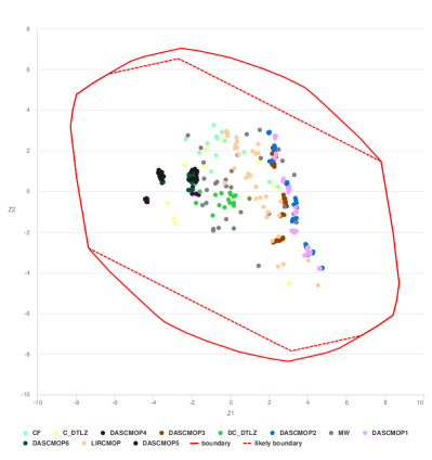
Figure 3: Distribution of the instances in 2D space by using the projection matrix in Equation (5). Instances are color-coded based on the source.

Figure 4 illustrates the number of algorithms that performed well on each instance, as a proxy of their difficulty. Darker colors of the points in the plot corresponds to fewer algorithms performing well. The figure suggests that the instances in the left area are generally easier to solve by most of the algorithms, especially the instances in the bottom-left of the plot.

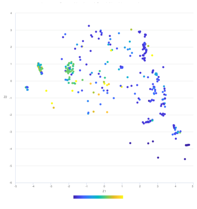
Figure 4: Number of algorithms performed well for each instance, where good performance means a normalized $HV$ within 1% of the best algorithm. The color scale corresponds to the total number of algorithms. A color closer to dark blue means fewer number of algorithms performed well.

IV-B Algorithms Footprints

Figure 5 shows the footprints of the algorithms in the instance space. An orange point means the algorithm performed badly compared to others on such instances, while blue represent good performance. We limit our analysis to only seven algorithms, as footprints reveal high similarity between many of them. ANSGAIII, NSGAII and MOEAD with the principle of constraint dominance, $\epsilon$-constraint, and stochastic ranking share similar footprints, as well as CMOEA_MS which depends on the principle of constraint dominance but sometimes includes the constraint violation as an objective. The footprints of this group are represented by the footprints of NSGAII in 5a, which shows that they are capable of providing relatively good performance in only a third of the instance space. Penalty based algorithms (PECNSGAII, PECMOEAD) 5b have similar footprints; both of them matched the best algorithm in instances located near the origin or on the bottom-left area. Whilst, MOEADDAE 5c, which uses two stages to relax the penalty factor, performed well in almost all the area covered by penalty based algorithms, and matched part of the first group footprints.

On the other hand, CTAEA, ToP, CCMO, and PPS have distinctive footprints. CTAEA and ToP have the lowest proportion of good performance, but they have different footprints. CTAEA 5d seems only capable of providing high quality solutions in easy to solve instances, while ToP 5e targeted instances that are rarely solved by previous algorithms. CCMO 5f and PPS 5g appear to be the only two algorithms performed well in a wide area of the instance space. Moreover, they have almost opposite footprints. Both algorithms use two strategies to handle constraints, the first one is considering objectives only, but for the second CCMO uses the principle of constraint dominance while PPS uses $\epsilon$-constraint. CCMO uses the two strategies in parallel by having two populations, while PPS uses them sequentially by applying the first strategy for several generations, then, applying the second strategy.

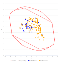
(a)

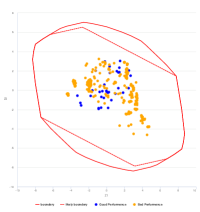
(b)

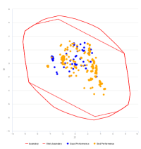
(c)

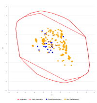
(d)

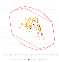
(e)

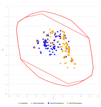
(f)

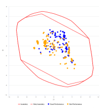
(g)

Figure 5: Seven algorithms footprints in the projected instance space, where good performance means a normalized $HV$ within 1% of the best algorithm.

IV-C Features Impact

Within the instance space, we can gain insights into an algorithm’s strength and weakness by examining the distribution of features across the space. Here, we present a subset of features that better explain how easy or difficult an instance is for at least one algorithm. Figures 6a and 4 show that instances that have high positive correlation between constraints and objectives are easier to solve, which suggests that the evolutionary trajectory of the search in those instances is not affected by the infeasible area; a search directed by objectives or constraints will probably lead directly to the optimal set of solutions. In addition, Figure 6b suggests that a smaller proportion of $cpo{\_}upo{\_}n$, representing isolation of the non-dominate set or a narrow feasible area, causes difficulty for most algorithms.

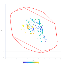
(a)

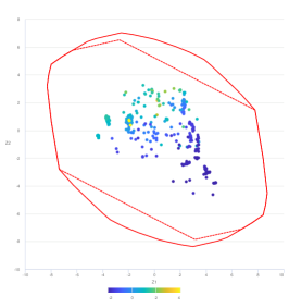
(b)

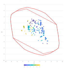
(c)

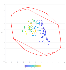
(d)

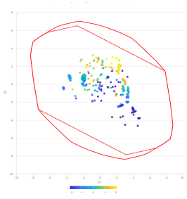
(e)

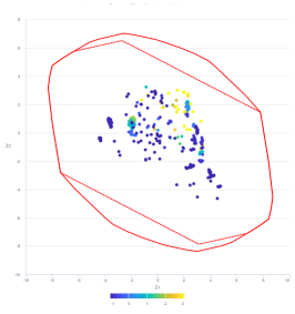
(f)

Figure 6: Distribution of normalized subset of features in the projected instance space. The color scale corresponds to normalized feature values.

Penalty-based algorithms do not have clear footprints in the represented instance space. The group represented by NSGAII, illustrated in Figure 5a, finds it easier to solve a problem if the average ratio of the distance between neighbors in the violation space to the distance in the decision space is not low, as shown in Figure 6c. This suggests the presence of large, neutral areas in the violation landscape. CCMO footprints seem to overlap with the distribution of $dist{\_}f{\_}dist{\_}x{\_}avg{\_}rws$, illustrated in Figure 6d. The higher this feature is, the more likely CCMO 5f will succeed. Moreover, CCMO seems to be capable of finding solutions in instances that have a low ratio of solutions in the ideal zone of one objective, as shown in Figure 6e, meaning that CCMO has the ability to find isolated optima. Although, this feature has the opposite impact on PPS, as observed in Figure 5g, suggesting that PPS is better suited to find diverse solutions when there are more local optimal solutions, which is also supported by $nhv{\_}avg{\_}rws$ as illustrated in Figure 6f. Furthermore, when there is negative correlation between constraints and objectives, illustrated in Figure 6a, PPS is one of the best performing algorithms. We can observe that the instances that have the highest conflict between constraints and objectives, are the instances that ToP was capable to excel at, as shown in Figure 5e.

IV-D ISA-based Algorithm Selection

In the final phase of our investigation, we focus on algorithm selection using a support vector machine (SVM). Figure 7 presents the SVM selection results generated by the MATILDA web tools [48]. The figure shows that hyper-strategies are more likely to be selected by the SVM model because they surpassed others in larger and clearer regions. The instance space is almost divided between CCMO and PPS, however, there are small area in the bottom-right that predicted to be solved mostly by ToP. However, this area was not easy to solve by almost all the algorithms, as observed in Figure 5. Our analysis of the instances in this area found that either there are no feasible solutions, or the HV of the set found by algorithms is approximately zero. Therefore, we conclude that the selection in this area is not accurate.

In addition, figure 8 describes the accuracy and precision of SVM selection model for each algorithm individually. The results validate the accuracy of the overall model. They illustrate that CCMO and PPS have high accuracy and precision, however, ToP has low precision. In addition, the metrics show that the quality of the algorithm selection model based on the selected features correlate with the clarity of the visualized footprints. For example, PECMOEAD, CTAEA, and ToP have poor SVM metrics values, and they do not have clear footprints on the projected instance space.

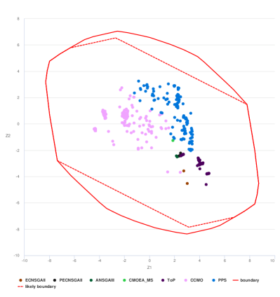
Figure 7: Algorithm recommendations by SVM selection model for the projected instance space.

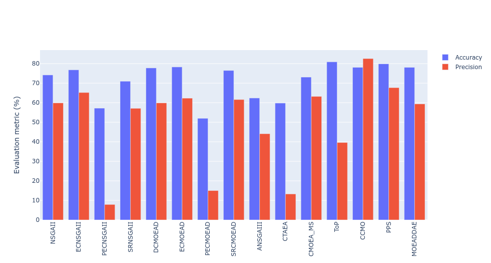
Figure 8: SVM selection model accuracy and precision for each algorithm.

V Conclusion

We have presented a detailed instance space analysis of CMOPs. Our primary motivation was to systematically evaluate and characterize the conditions where a selected CMOEA was expected to perform well based on the landscape analysis features of COMP instances. Firstly, we have identified COMP features in terms of three landscapes: the multi-objective landscape; the violation landscape and the multi-objective-violation landscape. Secondly, we have collected a large volume of meta-data encapsulating multiple benchmark problem instances and algorithms (including alternative constraint handling techniques). Finally, footprints corresponding to regions of varying algorithm performance were identified. This visual representation provides useful insights, helping to explain CMOPs characteristics and the strengths and weakness of a particular algorithm. In addition, a SVM selection model was then used to select the CMOEA with the best performance in a certain region of the instance space.

Our results show that some CMOEAs, CCMO and PPS in particular, have distinct footprints. CCMO and PPS employ hyper constraint handling techniques, where they use two strategies in two populations/stages. CCMO can effectively converge on isolated optima, whereas PPS generates more diversity when there is a large optimal set. Significantly, our analysis shows that most CMOEAs fail to evolve high quality solutions when there is negative correlation between constraints and objectives. Moreover, CTAEA and other penalty-based algorithms have no clear area of strength, which indicates that the available benchmarks lack examples on which these algorithms would outperform. Therefore, our selector is conservative, as it tends to pick between the two strongest algorithms, i.e., CCMO and PPS, with high precision.

It is widely acknowledged that any benchmark suite of problems should ideally test the efficacy of the optimizer. However, our analysis reveals a lack of diversity in the benchmark suites examined, with many instances sharing similar objective and/or constraint functions. Only a few instances provide a high proportion of constrained Pareto fronts to unconstrained ones, and fewer instances have a highly negative correlation between constraints and objectives. Despite the fact that those two features are challenging to most algorithms.

A wide range of existing and new features have been used in this work, however, they do not result in clear footprints for all algorithms. This, in turn, suggests that there is scope to further explore new features tailored specifically for CMOPs. Additionally, one of the objectives of benchmarking is to create problems that are representative of real-world problems [49]. Thus, we will investigate in future work where real-world problems fall within the instance space.

References

- [1] A. Kumar, G. Wu, M. Z. Ali, Q. Luo, R. Mallipeddi, P. N. Suganthan, and S. Das, “A Benchmark-Suite of real-World constrained multi-objective optimization problems and some baseline results,” Swarm Evol. Comput., vol. 67, p. 100961, 2021.
- [2] Z. Fan, W. Li, X. Cai, H. Li, C. Wei, Q. Zhang, K. Deb, and E. Goodman, “Difficulty Adjustable and Scalable Constrained Multiobjective Test Problem Toolkit,” Evol. Comput., vol. 28, no. 3, pp. 339–378, 2020.
- [3] F. Bogdan and V. Aljoša, “Multiobjective Optimization in the Presence of Constraints,” 2021.
- [4] Z. Fan, F. Yi, W. Li, J. Lu, X. Cai, and C. Wei, “A comparative study of constrained multi-objective evolutionary algorithms on constrained multi-objective optimization problems,” in 2017 IEEE Congr. Evol. Comput. (CEC 2017) - Proc., 2017, pp. 209–216.
- [5] O. Mersmann, B. Bischl, H. Trautmann, M. Preuss, C. Weihs, and G. Rudolph, “Exploratory landscape analysis,” in GECCO 2011 - Proc. 2011 Genet. Evol. Comput. Conf., 2011, pp. 829–836.
- [6] K. Smith-Miles, D. Baatar, B. Wreford, and R. Lewis, “Towards objective measures of algorithm performance across instance space,” Comput. Oper. Res., vol. 45, pp. 12–24, 2014.
- [7] E. Yap, M. A. Muñoz, K. Smith-Miles, and A. Liefooghe, “Instance Space Analysis of Combinatorial Multi-objective Optimization Problems,” in 2020 IEEE Congr. Evol. Comput. (CEC 2020) - Proc., 2020.
- [8] M. A. Muñoz and K. Smith-Miles, “Performance analysis of continuous black-box optimization algorithms via footprints in instance space,” Evol. Comput., vol. 25, pp. 529–554, 2017.
- [9] K. M. Malan, “A survey of advances in landscape analysis for optimisation,” Algorithms, vol. 14, no. 2, 2021.
- [10] P. Kerschke, H. Wang, M. Preuss, C. Grimme, A. H. Deutz, H. Trautmann, and M. T. Emmerich, “Search dynamics on multimodal multiobjective problems,” Evol. Comput., vol. 27, no. 4, pp. 577–609, 2018.
- [11] A. Liefooghe, S. Verel, B. Lacroix, A. C. Zǎvoianu, and J. McCall, “Landscape features and automated algorithm selection for multi-objective interpolated continuous optimisation problems,” in GECCO 2021 - Proc. 2021 Genet. Evol. Comput. Conf., 2021, pp. 421–429.
- [12] K. M. Malan, J. F. Oberholzer, and A. P. Engelbrecht, “Characterising constrained continuous optimisation problems,” in 2015 IEEE Congr. Evol. Comput. (CEC 2057) - Proc., 2015, pp. 1351–1358.
- [13] S. Poursoltan and F. Neumann, Ruggedness Quantifying for Constrained Continuous Fitness Landscapes. New Delhi: Springer India, 2015, pp. 29–50.
- [14] C. Picard and J. Schiffmann, “Realistic constrained multiobjective optimization benchmark problems from design,” IEEE Trans. Evol. Comput., vol. 25, no. 2, pp. 234–246, 2021.
- [15] A. Vodopija, T. Tušar, and B. Filipič, “Characterization of constrained continuous multiobjective optimization problems: A feature space perspective,” 2021, https://arxiv.org/abs/2109.04564.
- [16] K. Smith-Miles and M. A. Muñoz, “Instance space analysis for algorithm testing: Methodology and software tools,” 2021, http://dx.doi.org/10.13140/RG.2.2.33951.48805.
- [17] J. R. Rice, “The algorithm selection problem,” Adv. Comput., vol. 15, pp. 65–118, 1976.
- [18] D. H. Wolpert and W. G. Macready, “No free lunch theorems for optimization,” IEEE Trans. Evol. Comput., vol. 1, no. 1, pp. 67–82, 1997.
- [19] Z. Ma and Y. Wang, “Evolutionary constrained multiobjective optimization: Test suite construction and performance comparisons,” IEEE Trans. Evol. Comput., vol. 23, no. 6, pp. 972–986, 2019.
- [20] Q. Zhang, A. Zhou, S. Zhao, P. N. Suganthan, W. Liu, and S. Tiwari, “Multiobjective optimization Test Instances for the CEC 2009 Special Session and Competition,” The School of Computer Science and Electronic Engieering, University of Essex, Tech. Rep. CES-487, 2009.
- [21] H. Jain and K. Deb, “An evolutionary many-objective optimization algorithm using reference-point based nondominated sorting approach, part ii: Handling constraints and extending to an adaptive approach,” IEEE Trans. Evol. Comput., vol. 18, no. 4, pp. 602–622, 2014.
- [22] K. Li, R. Chen, G. Fu, and X. Yao, “Two-archive evolutionary algorithm for constrained multiobjective optimization,” IEEE Trans. Evol. Comput., vol. 23, no. 2, pp. 303–315, 2019.
- [23] Z. Fan, W. Li, X. Cai, H. Huang, Y. Fang, Y. You, J. Mo, C. Wei, and E. Goodman, “An improved epsilon constraint-handling method in MOEA/D for CMOPs with large infeasible regions,” Soft Comput., vol. 23, pp. 12 491–12 510, 2019.
- [24] P. Stadler, “Fitness landscapes,” in Biological Evolution and Statistical Physics, Lecture Notes in Physics. Berlin, Heidelberg: Springer-Verlag, 2002, pp. 183–204.
- [25] S. Vérel, A. Liefooghe, L. Vermeulen-Jourdan, and C. Dhaenens, “Analyzing the effect of objective correlation on the efficient set of mnk-landscapes,” in LION, 2011.
- [26] M. A. Muñoz, Y. Sun, M. Kirley, and S. K. Halgamuge, “Algorithm selection for black-box continuous optimization problems: A survey on methods and challenges,” Inf. Sci., vol. 317, pp. 224–245, 2015.
- [27] J. Knowles and D. Corne, “Instance generators and test suites for the multiobjective quadratic assignment problem,” in Evolutionary Multi-Criterion Optimization, C. M. Fonseca, P. J. Fleming, E. Zitzler, L. Thiele, and K. Deb, Eds. Berlin, Heidelberg: Springer Berlin Heidelberg, 2003, pp. 295–310.
- [28] H. E. Aguirre and K. Tanaka, “Working principles, behavior, and performance of moeas on mnk-landscapes,” Eur. J. Oper. Res., vol. 181, pp. 1670–1690, 2007.
- [29] A. Liefooghe, F. Daolio, S. Verel, B. Derbel, H. Aguirre, and K. Tanaka, “Landscape-Aware Performance Prediction for Evolutionary Multiobjective Optimization,” IEEE Trans. Evol. Comput., vol. 24, no. 6, pp. 1063–1077, 2019.
- [30] T. Jones and S. Forrest, “Fitness Distance Correlation as a Measure of Problem Difficulty for Genetic Algorithms,” in the 6th Int. Conf. Genet. Algorithms, 1995, pp. 184–192.
- [31] A. Liefooghe, S. Vérel, H. E. Aguirre, and K. Tanaka, “What makes an instance difficult for black-box 0-1 evolutionary multiobjective optimizers?” in Artif. Evol., 2013.
- [32] E. Yap, M. A. Muñoz, and K. Smith-Miles, “Informing multi-objective optimisation benchmark construction through instance space analysis,” 2022, https://www.researchgate.net/publication/358629148_Informing_multi-objective_optimisation_benchmark_construction_through_Instance_Space_Analysis.
- [33] K. Deb, A. Pratap, S. Agarwal, and T. Meyarivan, “A Fast and Elitist Multiobjective Genetic Algorithm: NSGA-II,” IEEE Trans. Evol. Comput., vol. 6, no. 2, pp. 182–197, 2002.
- [34] E. Zitzler and L. Thiele, “Multiobjective evolutionary algorithms: a comparative case study and the strength pareto approach,” IEEE Trans. Evol. Comput., vol. 3, pp. 257–271, 1999.
- [35] D. A. van Veldhuizen, “Multiobjective evolutionary algorithms: classifications, analyses, and new innovations,” Ph.D. dissertation, Air Force Institute of Technology, 1999.
- [36] Y. Tian, Y. Zhang, Y. Su, X. Zhang, K. C. Tan, and Y. Jin, “Balancing Objective Optimization and Constraint Satisfaction in Constrained Evolutionary Multiobjective Optimization,” IEEE Trans. Cybern., pp. 1–14, 2021.
- [37] Z. Fan, W. Li, X. Cai, H. Li, C. Wei, Q. Zhang, K. Deb, and E. D. Goodman, “Push and pull search for solving constrained multi-objective optimization problems,” Swarm Evol. Comput., vol. 44, pp. 665–679, 2019.
- [38] A. Angantyr, J. Andersson, and J.-O. Aidanpaa, “Constrained optimization based on a multiobjective evolutionary algorithm,” in 2003 IEEE Congr. Evol. Comput. (CEC 2003) - Proc., vol. 3, 2003, pp. 1560–1567 Vol.3.
- [39] M. A. Jan, N. Tairan, and R. A. Khanum, “Threshold based dynamic and adaptive penalty functions for constrained multiobjective optimization,” in 1st Int. Conf. Artif. Intell., Model. Simul. (AIMS 2013), Kota Kinabalu, Malaysia, 2013, pp. 49–54.
- [40] Q. Zhu, Q. Zhang, and Q. Lin, “A constrained multiobjective evolutionary algorithm with detect-and-escape strategy,” IEEE Trans. Evol. Comput., vol. 24, no. 5, pp. 938–947, 2020.
- [41] W. Ning, B. Guo, Y. Yan, X. Wu, J. Wu, and D. Zhao, “Constrained multi-objective optimization using constrained non-dominated sorting combined with an improved hybrid multi-objective evolutionary algorithm,” Eng. Optim., vol. 49, no. 10, pp. 1645–1664, 2017.
- [42] T. Runarsson and X. Yao, “Stochastic ranking for constrained evolutionary optimization,” IEEE Trans. Evol. Comput., vol. 4, no. 3, pp. 284–294, 2000.
- [43] Y. Tian, T. Zhang, J. Xiao, X. Zhang, and Y. Jin, “A coevolutionary framework for constrained multiobjective optimization problems,” IEEE Trans. Evol. Comput., vol. 25, no. 1, pp. 102–116, 2021.
- [44] Z.-Z. Liu and Y. Wang, “Handling constrained multiobjective optimization problems with constraints in both the decision and objective spaces,” IEEE Trans. Evol. Comput., vol. 23, no. 5, pp. 870–884, 2019.
- [45] E. Zitzler, D. Brockhoff, and L. Thiele, “The Hypervolume Indicator Revisited: On the Design of Pareto-compliant Indicators Via Weighted Integration,” in Evolutionary Multi-Criterion Optimization. EMO 2007. Lect. Notes Comput. Sci. Springer, Berlin, Heidelberg, 2007, vol. 4403.
- [46] C. Audet, S. L. Digabel, D. Cartier, J. Bigeon, and L. Salomon, “Performance indicators in multiobjective optimization,” Eur. J. Oper. Res., vol. 292, pp. 397–422, 2021.
- [47] Y. Tian, R. Cheng, X. Zhang, and Y. Jin, “PlatEMO: A MATLAB platform for evolutionary multi-objective optimization,” IEEE Comput. Intell. Mag., vol. 12, no. 4, pp. 73–87, 2017.
- [48] K. Smith-Miles, M. A. Munoz, and Neelofar, “Melbourne Algorithm Test Instance Library with Data Analytics (MATILDA),” 2020. [Online]. Available: https://matilda.unimelb.edu.au
- [49] T. Bartz-Beielstein, C. Doerr, J. Bossek, S. Chandrasekaran, T. Eftimov, A. Fischbach, P. Kerschke, M. López-Ibáñez, K. M. Malan, J. H. Moore, B. Naujoks, P. Orzechowski, V. Volz, M. Wagner, and T. Weise, “Benchmarking in optimization: Best practice and open issues,” CoRR, vol. abs/2007.03488, 2020.