Abstract

In our recent work, we introduced the reduced unified continuum formulation for vascular fluid-structure interaction (FSI) and demonstrated enhanced solver accuracy, scalability, and performance compared to conventional approaches. We further verified the formulation against Womersley’s deformable wall theory. In this study, we assessed its performance in a compliant patient-specific aortic model by leveraging 3D printing, 2D magnetic resonance imaging (MRI), and 4D-flow MRI to extract high-resolution anatomical and hemodynamic information from an in vitro flow circuit. To accurately reflect experimental conditions, we additionally enabled in-plane vascular motion at each inlet and outlet, and implemented viscoelastic external tissue support and vascular tissue prestressing. Validation of our formulation is achieved through close quantitative agreement in pressures, lumen area changes, pulse wave velocity, and early systolic velocities, as well as qualitative agreement in late systolic flow structures. Our validated suite of FSI techniques can be used to investigate vascular disease initiation, progression, and treatment at a computational cost on the same order as that of rigid-walled simulations. This study is the first to validate a cardiovascular FSI formulation against an in vitro flow circuit involving a compliant vascular phantom of complex patient-specific anatomy.

Key Terms: Fluid-structure interaction, Pulse wave velocity, Magnetic resonance imaging, Compliant 3D printing, In vitro validation

Abbreviations

CFD	computational fluid dynamics
CMM	coupled momentum method
FSI	fluid-structure interaction
GRE	gradient echo
LSE	least squares error
PC-MRI	phase contrast magnetic resonance imaging
PWV	pulse wave velocity
RANSAC	Random Sample Consensus
RUC	reduced unified continuum
SPGR	spoiled gradient echo MRI
TTF	time-to-foot

Glossary of Terms

Symbol	Name	Definition	SI Unit
$\Omega$	FSI domain	FSI domain	-
$\Omega^{f}$	fluid domain	fluid domain	-
$\Omega^{s}$	solid domain	solid domain	-
$\Gamma_{I}$	fluid-solid interface	interface between $\Omega^{s}$ and $\Omega^{f}$	-
$\Gamma_{W}$	solid outer wall	outer wall of $\Omega^{s}$	-
$\Gamma^{i}_{\mathrm{cap}}$	$i$-th annular solid cap	$i$-th annular solid cap	-
$\Gamma^{i}_{\mathrm{ring}}$	$i$-th solid ring	$i$-th solid ring on $\Gamma_{I}$	-
$\bm{n}^{s}$	solid unit outward normal	unit outward normal vector of $\Omega^{s}$	-
$\bm{u}^{s}$	solid displacement	solid displacement	m
$\bm{u}^{w}$	membrane displacement	membrane displacement on $\Gamma_{I}$	m
$\bm{v}^{s}$	solid velocity	solid velocity	m/s
$\rho^{s}$	solid density	solid density	kg/m3
$\bm{\sigma}^{s}$	solid Cauchy stress	solid Cauchy stress	N/m2
$\bm{\sigma}_{0}$	solid prestress	$\bm{\sigma}^{s}$ at imaging	N/m2
$\bm{b}^{s}$	solid body force	solid body force	N/kg
$\bm{\sigma}^{s,l}$	solid lamina Cauchy stress	$\bm{\sigma}^{s}$ in lamina coordinate system	N/m2
$\bm{u}^{s,l}$	solid lamina displacement	$\bm{u}^{s}$ in lamina coordinate system	m
$E$	Young’s modulus	Young’s modulus	N/m2
$\nu$	Poisson’s ratio	Poisson’s ratio	-
$k^{s}$	spring constant	external elastic support	kg/(m${}^{2}\cdot$ s2)
$c^{s}$	damping constant	external viscous support	kg/(m${}^{2}\cdot$ s)
$h^{s}$	wall thickness	wall thickness	m
$\bm{n}^{f}$	fluid unit outward normal	unit outward normal vector of $\Omega^{f}$	-
$\bm{v}^{f}$	fluid velocity	fluid velocity	m/s
$p^{f}$	fluid pressure	fluid pressure	N/m2
$\rho^{f}$	fluid density	fluid density	kg/m3
$\mu^{f}$	fluid dynamic viscosity	fluid dynamic viscosity	N $\cdot$ s/m2
$\bm{b}^{f}$	fluid body force	fluid body force	N/kg
$\bm{h}^{f}$	fluid boundary traction	fluid boundary traction	N
$T_{p}$	cardiac period	length of cardiac cycle	s

1 Introduction

As image-based computational fluid dynamics (CFD) and fluid-structure interaction (FSI) simulations continue to gain traction for predictive and personalized medicine, it is imperative that numerical CFD and FSI methods be verified and, furthermore, validated against in vivo and/or in vitro data. Phase contrast magnetic resonance imaging (PC-MRI), which encodes absolute velocities of coherent blood flow, was previously limited to unidirectional velocity encoding in 2D. Recent developments in 4D-flow MRI, however, have enabled three-directional velocity encoding over 3D volumes, paving the way for increasingly detailed numerical validation.

We recently developed a unified continuum formulation for FSI [25] that not only recovers important continuum models including viscous fluids and visco-hyperelatic solids [24], but is also well-behaved in both compressible and fully incompressible regimes. This unified continuum formulation was then simplified to a reduced unified continuum (RUC) formulation via consideration of three modeling assumptions for vascular FSI, namely the infinitesimal strain, thin-walled, and membrane assumptions [21]. The RUC formulation, which achieves monolithic coupling of the fluid and solid subproblems in an Eulerian frame, was found to offer computational cost as low as $1.3$ times that of rigid-walled CFD simulations [22]. While the coupled momentum method (CMM) [7] similarly embeds a linear elastic membrane into an Eulerian fluid subproblem, key theoretical and numerical differences exist with regard to the fluid-solid coupling, spatiotemporal discretization, vascular wall dynamics, and linear solver technology [21]. In our verification against Womersley’s deformable wall theory, we demonstrated notable agreement between analytical and numerical solutions. Given the overlap in assumptions in the RUC formulation and Womersley’s deformable wall theory, assessing the validity of our adopted assumptions in settings of practical clinical interest, particularly with complex anatomical geometries, remains necessary.

CFD simulations of the cardiovascular system have commonly been validated against in vivo velocities from either 2D cine PC-MRI [28, 17, 6] or 4D-flow MRI [32, 31, 2]. Numerical validation can alternatively be performed against in vitro MRI of experimental flow phantoms embedded in benchtop circuits to assess effects of various parameters, including boundary conditions, anatomical geometries, and wall mechanical properties, on the flow behavior and solver performance. Constrained by limitations in fabrication methods, these in vitro experiments have until recently employed rigid flow phantoms constructed from photoreactive resin [19, 35, 4, 14]. Alastruey et al. [1] and Kung et al. [18] were among the first to perform in vitro FSI validation on compliant flow phantoms of idealized geometries that were fabricated from silicone dip-spin coating or hand-painting. Numerous other flow circuits with compliant flow phantoms fabricated from silicone, polyurethane, or latex [34, 16, 15] have also been engineered to investigate cardiovascular hemodynamics in health and disease and to further assess the performance of implantable devices. Recent advances in 3D printing techniques [13], including PolyJet and stereolithography, now enable rapid, repeatable printing of compliant patient-specific flow phantoms from novel photopolymers [5, 11, 36] without the need for laborious procedures. Importantly, mechanical characterization of these cost-effective phantoms can be performed to inform FSI validation studies. Nonetheless, to our knowledge, no previous studies have validated cardiovascular FSI formulations against in vitro flow circuits involving compliant patient-specific vascular phantoms.

In a previously published study [36], we demonstrated the use of novel compliant 3D printing to fabricate patient-specific aortic phantoms of three stiffness values, which were then embedded in an MRI-compatible flow circuit under physiological hemodynamic conditions. In our current study, we focus only on the most compliant phantom and assess the RUC formulation by drawing direct comparisons to the experimentally measured three-component 3D velocities, flow rates, pressures, luminal area changes, and pulse wave velocity. Effects of selected boundary conditions are also assessed.

2 Materials and Methods

In this section, we summarize the experimental methods [36] adopted to acquire the in vitro MRI data as well as the numerical methods employed to simulate the flow circuit.

2.1 3D-Printed Aortic Flow Phantom

Under a protocol approved by the Stanford Institutional Review Board, an in vivo chest 4D-flow MRI of a 50-year-old male subject was acquired with informed consent and subsequently used to construct a 3D anatomical model of the thoracic aorta (Figure 1A) in the open-source software package SimVascular [20]. We modeled the ascending aortic inlet (inlet) and four outlets, namely the brachiocephalic artery (BCA), left common carotid artery (LCA), left subclavian artery (LSA), and descending aorta (outlet). To define the outer wall surface, Meshmixer (Autodesk) was used to extrude surface mesh nodes by the wall thickness $h^{s}=0.2$ cm. Each inlet and outlet was finally extended by $2$ cm to facilitate tubing connections in the flow circuit.

A PolyJet photopolymerization 3D printer (Stratasys) was used to print the phantom from a material blend of the Agilus30 and VeroClear photopolymers (Figure 1B). Three dumbbell-shaped samples were additionally printed for uniaxial tensile testing to 50% peak strain at a strain rate of 25% s^-1. The tangential Young’s modulus at a nominal stress corresponding to the experimentally measured mean pressure ($56$ mm Hg) was determined to be $1.27\times 10^{7}$ dyn/cm².

2.2 MRI-Compatible In Vitro Flow Circuit

The 3D-printed aortic flow phantom was embedded in a gel block (Figure 1C) to ensure repeatable positioning and to provide a static “tissue” reference for eddy current phase offset correction. Components of the in vitro flow circuit included an MRI-compatible programmable flow pump (Shelley Medical Imaging Technologies), a fluid reservoir, sealed air compression chambers serving as capacitance elements, and pinch valves distal to the outlets to model distal vascular resistance. A 40%-60% glycerol-water mixture was used to mimic blood density and viscosity. Pressure transducers (Millar) were inserted at inlet and outlet, and an ultrasonic flow probe (Transonic Systems) was clamped at outlet. Resistance and capacitance parameters were tuned to achieve physiological pressures and flow splits prior to removal of the pressure and flow transducers.

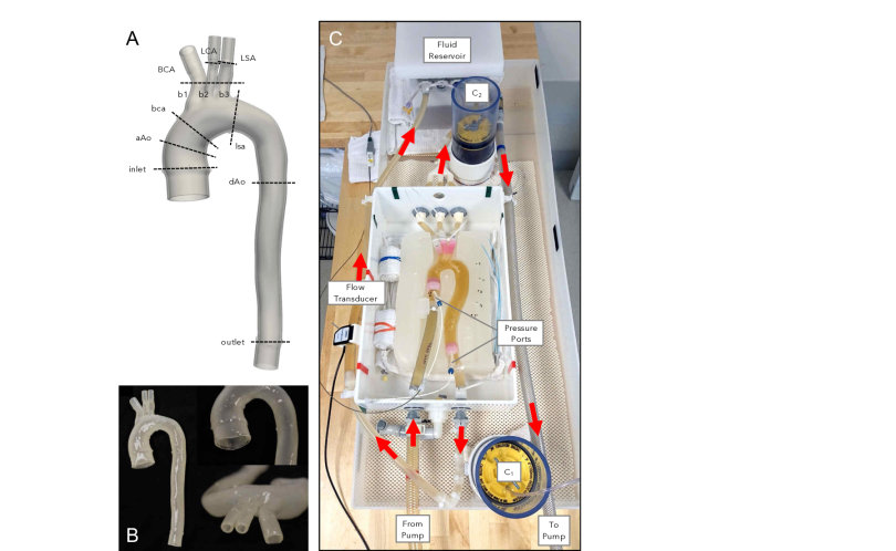
Figure 1: (A) Print-ready 3D STL model of a patient-specific thoracic aorta, annotated with the caps and landmark slices for 2D cine PC-MRI and 2D cine GRE MRI. (B) The resulting compliant 3D-printed flow phantom with $2$-cm extensions on all five caps to facilitate connection to custom barbed model-tubing transition elements. (C) MRI-compatible in vitro flow circuit consisting of a programmable flow pump, a fluid reservoir, tubing with pinch valves serving as resistance elements, and two sealed air compression chambers ($C_{1}$, $C_{2}$) serving as capacitance elements. A flow transducer and two pressure transducers were inserted for resistance and capacitance tuning prior to transfer of the flow circuit into the MRI scanner. Red arrows indicate the direction of flow.

2.3 MRI Acquisitions

All imaging experiments were performed with a 3 Tesla MRI scanner (Siemens Healthineers) at a temporal resolution of $0.02$ s. 3D spoiled gradient echo (SPGR) was first performed at a steady flow of $71.2$ mL/s to capture high-resolution anatomical information. Subsequently, 2D cine PC-MRI, 2D cine gradient echo (GRE) MRI, and 4D-flow MRI were performed under pulsatile flow, programmed to achieve mean and peak flow rates of $71.2$ mL/s and $300$ mL/s, respectively, at a cardiac period $T_{p}=1.0$ s. The $7$ planes at which 2D cine PC-MRI and 2D cine GRE MRI were performed (Figure 1A) corresponded to the ascending aortic inlet (inlet), ascending aorta (aAo), arch proximal to the brachiocephalic artery (bca), the three neck arteries (b1, b2, b3), arch distal to the left subclavian artery (lsa), mid-descending aorta (dAo), and the descending aortic outlet (outlet). 4D-flow scans were corrected for artifacts produced by Maxwell terms, gradient nonlinearity, and eddy currents.

2.4 Image Analysis

Time-varying lumen contours were automatically tracked in the 2D cine GRE scans. Time-varying 2D cine PC-MRI velocities were then masked with these lumen contours and integrated into flow rate waveforms.

To determine the pulse wave velocity (PWV), we analyzed temporal shifts in the time-to-foot (TTF) [29] of flow rate waveforms. Specifically, lumen contours at $50$ equidistant normal slices along the descending aortic centerline (from lsa to outlet) were automatically tracked in the 4D-flow magnitude images. Time-varying 4D-flow MRI velocities were then masked with these lumen contours and integrated into flow rate waveforms. The TTF for each flow rate waveform was determined to be the time of intersection between the following two lines: (i) horizontal line through the waveform’s diastolic value, and (ii) line through the waveform’s upslope points at 20% and 80% of the way from the diastolic value to its peak flow rate. The PWV was finally defined to be the slope of the linear regression line fitted to all $50$ TTFs plotted against the corresponding centerline positions. In addition to a least squares error (LSE) regression, a linear regression was also performed using Random Sample Consensus (RANSAC) to exclude outliers.

2.5 Computational Model and Mesh Generation

We employed SimVascular to segment the steady deformed configuration of the aortic phantom from the 3D SPGR scan. The inlet and outlets were truncated to exclude the artificial $2$-cm cap extensions (Figure 2). TetGen was used to discretize the 3D anatomical model with linear tetrahedral elements and three boundary layers at a layer decreasing ratio of $0.5$. Using meshes up to $3.92\times 10^{6}$ elements, a mesh convergence study was performed for steady-state diastolic simulations. Based on a tolerance criterion of $3\%$ variation across all cap pressures and flows, we settled on a mesh with $1.98\times 10^{6}$ elements and $3.35\times 10^{5}$ nodes.

2.6 RUC Formulation for Vascular FSI

2.6.1 Strong-Form FSI Problem

We consider a domain $\Omega\subset\mathbb{R}^{3}$ admitting a non-overlapping subdivision $\overline{\Omega}=\overline{\Omega^{f}\cup\Omega^{s}}$, $\emptyset=\Omega^{f}\cap\Omega^{s}$, in which $\Omega^{f}$ and $\Omega^{s}$ represent the fluid and solid subdomains with unit outward normal vectors $\bm{n}^{f}$ and $\bm{n}^{s}$, respectively. The fluid-solid interface $\Gamma_{I}$ is a two-dimensional manifold on which $\bm{n}^{f}=-\bm{n}^{s}$.

Under the infinitesimal strain assumption, the solid governing equations posed in $\Omega^{s}$ are as follows,

$$\bm{0}=\frac{d\bm{u}^{s}}{dt}-\bm{v}^{s},$$

$$\bm{0}=\rho^{s}\frac{d\bm{v}^{s}}{dt}-\nabla\cdot\bm{\sigma}^{s}-\rho^{s}\bm{b}^{s},$$

where $\bm{u}^{s}$, $\bm{v}^{s}$, $\rho^{s}$, $\bm{\sigma}^{s}$, and $\bm{b}^{s}$ are the solid displacement, velocity, density, Cauchy stress, and body force per unit mass, respectively. Considering isotropic linear elasticity, we express the constitutive relation as follows in the lamina coordinate system,

$$\bm{\sigma}^{s,l}=\mathbb{C}^{s,l}\bm{\epsilon}^{l}(\bm{u}^{s,l}),\quad\mathbb{C}^{s,l}:=2\mu^{s}(\bm{x}^{l})\mathbb{I}+\lambda^{s}(\bm{x}^{l})\bm{I}\otimes\bm{I},\quad\bm{\epsilon}^{l}(\bm{u}^{s,l}):=\frac{1}{2}\left(\nabla\bm{u}^{s,l}+\left(\nabla\bm{u}^{s,l}\right)^{T}\right),$$

where $\bm{\sigma}^{s,l}$ and $\bm{\epsilon}^{l}(\bm{u}^{s,l})$ are respectively the Cauchy stress and infinitesimal strain in the lamina coordinate system, $\bm{I}$ is the second-order identity tensor, $\mathbb{I}$ is the fourth-order symmetric identity tensor, and $\mu^{s}$ and $\lambda^{s}$ are the Lamé parameters. In Voigt notation,

$$\bm{\sigma}^{s,l}=\left[\sigma_{11}^{s,l},\sigma_{22}^{s,l},\sigma_{12}^{s,l},\sigma_{23}^{s,l},\sigma_{31}^{s,l}\right]^{T},$$

$$\bm{\epsilon}^{l}(\bm{u}^{s,l})=\left[\epsilon_{11}^{l},\epsilon_{22}^{l},2\epsilon_{12}^{l},2\epsilon_{23}^{l},2\varepsilon_{31}^{l}\right]^{T}=\left[u_{1,1}^{s,l},u_{2,2}^{s,l},u_{1,2}^{s,l}+u_{2,1}^{s,l},u_{3,2}^{s,l},u_{3,1}^{s,l}\right]^{T},$$

$$\mathbb{C}^{s,l}=\frac{E}{(1-\nu^{2})}\begin{bmatrix}1&\nu&&&\\[2.84526pt] \nu&1&&&\\[2.84526pt] &&\displaystyle\frac{1-\nu}{2}&&\\[2.84526pt] &&&\kappa\displaystyle\frac{(1-\nu)}{2}&\\[2.84526pt] &&&&\kappa\displaystyle\frac{(1-\nu)}{2}\\[2.84526pt] \end{bmatrix},$$

where $E$ is the Young’s modulus, $\nu$ is the Poisson’s ratio, and $\kappa=5/6$ is the shear correction factor. Experimentally determined wall properties were uniformly prescribed: $E=1.27\times 10^{7}$ dyn/cm², $h^{s}=0.2$ cm, $\rho^{s}=1.0$ g/cm³, $\nu=0.5$. Using a rotation matrix $\bm{Q}$ transforming global coordinates to lamina coordinates, we then compute the Cauchy stress in the global coordinate system as $\bm{\sigma}^{s}=\bm{Q}^{T}\bm{\sigma}^{s,l}\bm{Q}$.

In the fluid subdomain $\Omega^{f}$, we consider an incompressible Newtonian fluid governed by the following equations in an Eulerian frame,

$$\bm{0}=\rho^{f}\frac{\partial\bm{v}^{f}}{\partial t}+\rho^{f}\bm{v}^{f}\cdot\nabla\bm{v}^{f}-\nabla\cdot\bm{\sigma}^{f}_{\mathrm{dev}}+\nabla p^{f}-\rho^{f}\bm{b}^{f},$$

$$0=\nabla\cdot\bm{v}^{f},$$

where $\bm{v}^{f}$, $p^{f}$, $\rho^{f}$, $\mu^{f}$, and $\bm{b}^{f}$ are the fluid velocity, pressure, density, dynamic viscosity, and body force per unit mass, respectively; $\bm{\sigma}^{f}_{\mathrm{dev}}$ and $\bm{\varepsilon}_{\mathrm{dev}}$ are the deviatoric parts of the Cauchy stress and rate-of-strain,

$$\bm{\sigma}^{f}_{\mathrm{dev}}:=2\mu^{f}\bm{\varepsilon}_{\mathrm{dev}}(\bm{v}^{f}),\quad\bm{\varepsilon}_{\mathrm{dev}}(\bm{v}^{f}):=\frac{1}{2}\left(\nabla\bm{v}^{f}+\left(\nabla\bm{v}^{f}\right)^{T}\right)-\frac{1}{3}\nabla\cdot\bm{v}^{f}\bm{I},$$

and the fluid Cauchy stress is given by $\bm{\sigma}^{f}:=\bm{\sigma}^{f}_{\mathrm{dev}}-p^{f}\bm{I}$. In this work, we set the fluid density $\rho^{f}$ to $1.06$ g/cm³ and fluid viscosity $\mu^{f}$ to $0.04$ Poise.

The strong-form FSI problem is completed with the kinematic and dynamic coupling conditions enforcing the continuity of velocity and traction on $\Gamma_{I}$, respectively,

$$\bm{v}^{f}=\bm{v}^{s},\qquad\bm{\sigma}^{f}\bm{n}^{f}=-\bm{\sigma}^{s}\bm{n}^{s}.$$

2.6.2 Numerical Boundary Conditions

The boundary of the solid subdomain can be decomposed as $\partial\Omega^{s}=\Gamma_{I}\cup\Gamma_{W}\cup\bigcup_{i=1}^{\mathrm{n}_{\mathrm{cap}}}\Gamma^{i}_{\mathrm{cap}}$, where $\Gamma_{W}$ represents the outer wall, $\Gamma^{i}_{\mathrm{cap}}$ represents the $i$-th annular cap surface, and $\mathrm{n}_{\mathrm{cap}}=5$ represents the number of cap surfaces. While $\Gamma_{W}$ has conventionally been modeled as a stress-free surface, a Robin boundary condition was recently introduced to represent the viscoelastic behavior of tissues and organs surrounding the modeled vasculature [30]. To model the surrounding gel block, we imposed $\bm{\sigma}^{s}\bm{n}^{s}=-k^{s}\bm{u}^{s}-c^{s}\bm{v}^{f}$ on $\Gamma_{W}$, where the spring constant $k^{s}=0$ g/(cm${}^{2}\cdot$ s²) and damping constant $c^{s}=3.0\times 10^{5}$ g/(cm${}^{2}\cdot$ s) were determined to best match experimental relative luminal area changes.

Furthermore, most vascular FSI simulations have enforced clamping, or zero displacements, at all inlets and outlets of the solid subdomain, yet the phantom inlet and outlets here were not experimentally clamped, given the $2$-cm extensions beyond the domain of interest. More recently, studies have relaxed this displacement constraint to enable either purely radial motion [8] or in-plane motion [3]. We similarly enabled in-plane motion on all caps by applying inclined ‘roller’ boundary conditions on the associated displacements as follows,

$$\bm{u}^{s}\cdot\bm{n}^{s}=0\quad\mbox{ and }\quad\bm{\sigma}^{s}\bm{n}^{s}-\left(\bm{\sigma}^{s}\bm{n}^{s}\cdot\bm{n}^{s}\right)\bm{n}^{s}=\bm{0},\quad\mbox{ on }\Gamma^{i}_{\mathrm{cap}}\quad\mbox{ for }i=1,\cdots,5.$$

To constrain degrees of freedom in skew directions [10], a skew coordinate system was established for each cap using $\bm{n}^{s}$ and two orthonormal vectors tangential to $\Gamma^{i}_{\mathrm{cap}}$. All associated equations were solved in the skew coordinate system, and solutions for the associated degrees of freedom were subsequently rotated back into the global coordinate system.

The boundary of the fluid subdomain can be decomposed as $\partial\Omega^{f}=\Gamma_{I}\cup\bigcup_{k=1}^{\mathrm{n}_{g}}\Gamma^{k}_{g}\cup\bigcup_{l=1}^{\mathrm{n}_{h}}\Gamma^{l}_{h}$, where boundary surface $\Gamma^{k}_{g}$ represents the $k$-th surface prescribed with Dirichlet data $\bm{g}^{k}(\bm{x},t)$ as $\bm{v}^{f}=\bm{g}^{k}(\bm{x},t)$, and $\Gamma^{l}_{h}$ represents the $l$-th surface prescribed with Neumann data $-P^{l}(t)$ as $\bm{\sigma}^{f}\bm{n}^{f}=-P^{l}(t)\bm{n}^{f}$. Here, we imposed Dirichlet conditions on inlet and the three neck artery outlets (BCA, LCA, and LSA) and a Neumann condition on outlet, yielding $\mathrm{n}_{g}=4$ and $\mathrm{n}_{h}=1$. In the remainder of this work, we eliminate the superscript $l$ for the Neumann boundary to simplify notation.

To prescribe time-varying velocity fields on inlet, we leveraged the three-component velocities from 4D-flow MRI rather than the unidirectional, through-plane velocities from 2D cine PC-MRI. Given the different coordinate systems across the various imaging sequences, 4D-flow and 2D cine GRE scans were first registered to the computational mesh via rigid coherent point drift. Time-varying inlet lumen contours from 2D cine GRE were then used to mask the 4D-flow velocities. To map these deforming luminal domains onto the stationary inlet surface mesh, a piecewise linear transformation was defined to map each experimental lumen contour to the boundary of the inlet mesh. The same piecewise linear transformation was then applied to the luminal domain of the masked inlet velocity profile, and the resulting velocity profile was interpolated onto the inlet mesh with a Gaussian kernel. Linear interpolation of the velocity fields was performed between consecutive temporal frames.

Despite use of the gel block to ensure repeatable phantom positioning, deformations were experimentally introduced, given the small size of the neck arteries and compliance of the phantom. The rigid registrations therefore yielded visible (though small) misalignment of the neck arteries, precluding assignment of 4D-flow velocity fields on the three corresponding outlets (BCA, LCA, LSA). Experimental b1, b2, and b3 flow rates integrated from 2D cine PC-MRI velocities were therefore respectively prescribed at BCA, LCA, and LSA with idealized parabolic velocity profiles. Lastly, experimental outlet transducer pressures were used to generate the functional form of $P(t)$ prescribed at outlet.

2.6.3 Discrete FSI Formulation

The semi-discrete formulation is constructed with the residual-based variational multiscale formulation. Considering a conforming mesh across $\Gamma_{I}$ immediately guarantees strong satisfaction of the kinematic coupling condition and weak satisfaction of the dynamic coupling condition.

Under a thin-walled assumption, the three-dimensional elastodynamic problem in $\Omega^{s}$ collapses to a two-dimensional problem posed on the fluid-solid interface $\Gamma_{I}$. Correspondingly, the outer wall $\Gamma_{W}$ collapses onto $\Gamma_{I}$, and annular surface $\Gamma^{i}_{\mathrm{cap}}$ collapses into a one-dimensional ring $\Gamma^{i}_{\mathrm{ring}}:=\Gamma_{I}\cap\Gamma^{i}_{\mathrm{cap}}$. Let $\bm{u}^{w}_{h}$ be the membrane displacement on $\Gamma_{I}$ and $\mathcal{S}^{w}_{\bm{u}}$ be its trial solution space. Let $\mathcal{S}_{\bm{v}}^{f}$ and $\mathcal{S}_{p}^{f}$ denote the trial solution spaces for the fluid velocity and pressure; let $\mathcal{V}_{\bm{v}}^{f}$ and $\mathcal{V}_{p}^{f}$ be their corresponding test function spaces. The semi-discrete FSI formulation posed only in $\Omega^{f}$ on a stationary mesh is then stated as follows. Find $\bm{y}_{h}(t):=\left\{\bm{u}^{w}_{h}(t),\bm{v}_{h}^{f}(t),p_{h}^{f}(t)\right\}\in\mathcal{S}^{w}_{\bm{u}}\times\mathcal{S}_{\bm{v}}^{f}\times\mathcal{S}_{p}^{f}$ such that $\forall\left\{\bm{w}_{h}^{f},q_{h}^{f}\right\}\in\mathcal{V}_{\bm{v}}^{f}\times\mathcal{V}_{p}^{f}$,

$$\mathbf{B}_{\mathrm{k}}\left(\dot{\bm{y}}_{h},\bm{y}_{h}\right)=\bm{0},$$

$$\mathbf{B}_{\mathrm{m}}\left(\bm{w}_{h}^{f};\dot{\bm{y}}_{h},\bm{y}_{h}\right):=\mathbf{B}^{w}_{\mathrm{m}}\left(\bm{w}_{h}^{f};\dot{\bm{y}}_{h},\bm{y}_{h}\right)+\mathbf{B}^{f}_{\mathrm{m}}\left(\bm{w}^{f}_{h};\dot{\bm{y}}^{f}_{h},\bm{y}^{f}_{h}\right)=0,$$

$$\mathbf{B}_{\mathrm{c}}\left(q^{f}_{h};\dot{\bm{y}}_{h},\bm{y}_{h}\right):=\mathbf{B}_{\mathrm{c}}\left(q_{h}^{f};\dot{\bm{y}}_{h}^{f},\bm{y}_{h}^{f}\right)=0,$$

where

$$\mathbf{B}_{\mathrm{k}}\left(\dot{\bm{y}}_{h},\bm{y}_{h}\right):=\frac{d\bm{u}^{w}_{h}}{dt}-\bm{v}^{f}_{h},\qquad\mbox{ on }\Gamma_{I},$$

$$\mathbf{B}^{w}_{\mathrm{m}}\left(\bm{w}_{h}^{f};\dot{\bm{y}}_{h},\bm{y}_{h}\right):=\int_{\Gamma_{I}}\bm{w}_{h}^{f}\cdot\rho^{s}h^{s}\left(\frac{d\bm{v}_{h}^{f}}{dt}-\bm{b}^{s}\right)d\Gamma+\int_{\Gamma_{I}}h^{s}\bm{\epsilon}(\bm{w}_{h}^{f}):\Big{(}\bm{\sigma}^{s}(\bm{u}_{h}^{w})+\bm{\sigma}_{0}\Big{)}d\Gamma$$

$$\hskip 79.66771pt+\int_{\Gamma_{I}}c^{s}\bm{w}_{h}^{f}\cdot\bm{v}^{f}d\Gamma,$$

$$\mathbf{B}^{f}_{\mathrm{m}}\left(\bm{w}_{h}^{f};\dot{\bm{y}}_{h}^{f},\bm{y}_{h}^{f}\right):=\int_{\Omega^{f}}\bm{w}_{h}^{f}\cdot\rho^{f}\left(\frac{\partial\bm{v}_{h}^{f}}{\partial t}+\bm{v}_{h}^{f}\cdot\nabla\bm{v}_{h}^{f}-\bm{b}^{f}\right)d\Omega-\int_{\Omega^{f}}\nabla\cdot\bm{w}_{h}^{f}p_{h}^{f}d\Omega$$

$$\hskip 79.66771pt+\int_{\Omega^{f}}2\mu^{f}\bm{\varepsilon}(\bm{w}_{h}^{f}):\bm{\varepsilon}(\bm{v}_{h}^{f})d\Omega-\int_{\Omega^{f\prime}}\nabla\bm{w}_{h}^{f}:\left(\rho^{f}\bm{v}^{\prime}\otimes\bm{v}_{h}^{f}\right)d\Omega$$

$$\hskip 79.66771pt+\int_{\Omega^{f\prime}}\nabla\bm{v}_{h}^{f}:\left(\rho^{f}\bm{w}_{h}^{f}\otimes\bm{v}^{\prime}\right)d\Omega-\int_{\Omega^{f\prime}}\nabla\bm{w}_{h}^{f}:\left(\rho^{f}\bm{v}^{\prime}\otimes\bm{v}^{\prime}\right)d\Omega$$

$$\hskip 79.66771pt-\int_{\Omega^{f\prime}}\nabla\cdot\bm{w}_{h}^{f}p^{\prime}d\Omega+\int_{\Gamma_{h}}\bm{w}_{h}^{f}\cdot\bm{n}^{f}P(t)d\Gamma-\int_{\Gamma_{h}}\rho^{f}\beta\left(\bm{v}_{h}^{f}\cdot\bm{n}^{f}\right)_{-}\bm{w}_{h}^{f}\cdot\bm{v}_{h}^{f}d\Gamma,$$

$$\mathbf{B}_{\mathrm{c}}\left(q_{h}^{f};\dot{\bm{y}}_{h}^{f},\bm{y}_{h}^{f}\right):=\int_{\Omega^{f}}q_{h}^{f}\nabla\cdot\bm{v}_{h}^{f}d\Omega-\int_{\Omega^{f\prime}}\nabla q_{h}^{f}\cdot\bm{v}^{\prime}d\Omega,$$

and

$$\bm{v}^{\prime}:=-\bm{\tau}_{M}\left(\rho^{f}\frac{\partial\bm{v}_{h}^{f}}{\partial t}+\rho^{f}\bm{v}_{h}^{f}\cdot\nabla\bm{v}_{h}^{f}+\nabla p_{h}^{f}-\mu^{f}\Delta\bm{v}_{h}^{f}-\rho^{f}\bm{b}^{f}\right),\quad p^{\prime}:=-\tau_{C}\nabla\cdot\bm{v}_{h}^{f},$$

$$\bm{\tau}_{M}:=\tau_{M}\bm{I}_{3},\quad\tau_{M}:=\frac{1}{\rho^{f}}\left(\frac{\mathrm{C}_{\mathrm{T}}}{\Delta t^{2}}+\bm{v}_{h}^{f}\cdot\bm{G}\bm{v}_{h}^{f}+\mathrm{C}_{\mathrm{I}}\left(\frac{\mu^{f}}{\rho^{f}}\right)^{2}\bm{G}:\bm{G}\right)^{-\frac{1}{2}},\quad\tau_{C}:=\frac{1}{\tau_{M}\textup{tr}\bm{G}},$$

$$G_{ij}:=\sum_{k=1}^{3}\frac{\partial y_{k}}{\partial x_{i}}M_{kl}\frac{\partial y_{l}}{\partial x_{j}},\quad\bm{M}=[M_{kl}]=\frac{\sqrt[3]{2}}{2}\begin{bmatrix}2&1&1\\ 1&2&1\\ 1&1&2\end{bmatrix},$$

$$\bm{G}:\bm{G}:=\sum_{i,j=1}^{3}G_{ij}G_{ij},\quad\textup{tr}\bm{G}:=\sum_{i=1}^{3}G_{ii},\quad\left(\bm{v}_{h}^{f}\cdot\bm{n}^{f}\right)_{-}:=\frac{\bm{v}_{h}^{f}\cdot\bm{n}^{f}-|\bm{v}_{h}^{f}\cdot\bm{n}^{f}|}{2}.$$

The prestress $\bm{\sigma}_{0}$ in $\mathbf{B}^{w}_{\mathrm{m}}$ that balances the in vivo blood pressure and viscous traction at the imaged configuration can be determined through a fixed-point algorithm [12, 21], and $\beta$ in the backflow stabilization term in $\mathbf{B}^{f}_{\mathrm{m}}$ is set to $0.2$. In the definition of $G_{ij}$, $\bm{y}=\left\{y_{i}\right\}_{i=1}^{3}$ are natural coordinates in the parent domain, and $\bm{M}$ is introduced to yield node-numbering-invariant definitions of $\tau_{M}$ and $\tau_{C}$ for simplex elements. $C_{I}$ and $C_{T}$ are taken to be $36$ and $4$ for linear tetrahedral elements.

The generalized-$\alpha$ method [21, 23] is then applied for temporal discretization of the above semi-discrete FSI formulation. In this work, the time step size was uniformly selected as $T_{p}/1000$.

2.6.4 Numerical Simulation Strategies

The fully discrete scheme was solved iteratively via a predictor multi-corrector algorithm. To reduce the size of the associated linear system and enable effective block preconditioning [21, 27], we leveraged the special block structure of the fully consistent tangent matrix to develop a segregated algorithm. Our block preconditioner was previously shown to exhibit enhanced robustness and scalability as compared to alternative preconditioners in applications spanning hyperelasticity, viscous fluids, and FSI [21, 26].

To reflect the steady configuration captured by the 3D SPGR scan, we initialized our simulation in the following steps. A rigid-walled CFD simulation was first performed with a prescribed steady inflow of $71.2$ mL/s to determine the corresponding fluid traction $\bm{h}^{f}$. Resistance boundary conditions were prescribed at all four outlets, tuned to achieve the experimental outflow distribution ($18.0\%$ BCA, $4.9\%$ LCA, $3.8\%$ LSA, $73.3\%$ outlet) and mean experimental pressures (inlet $56$ mm Hg, outlet $55$ mm Hg). The resulting $\bm{h}^{f}$ was then used in the fixed-point algorithm to determine $\bm{\sigma}_{0}$. With the vascular wall appropriately prestressed, we performed a steady-state FSI simulation prescribed with steady diastolic boundary conditions corresponding to $t=0$, from which we initialized our pulsatile simulation. Three cardiac cycles were simulated to ensure convergence to a limit cycle, and only the third cycle was analyzed.

Comparisons between experimental and simulated velocity fields were made possible by sampling the 4D-flow velocity fields onto the computational mesh. With the same TTF approach discussed in Section 2.4, we computed the numerical PWV using simulated pressure waveforms at the same $50$ normal slices. We note that in contrast to the use of flow waveforms to compute the experimental PWV, pressure waveforms were instead used to compute the numerical PWV due to their uniformity in waveform shape.

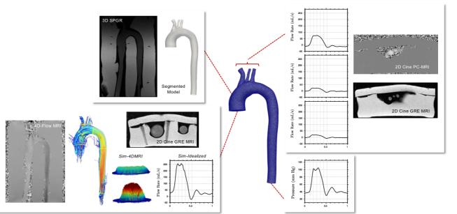
Figure 2: Schematic of numerical simulation methods incorporating data from four MRI sequences. The anatomical model was segmented from the 3D SPGR scan. Velocities from 2D cine PC-MRI were integrated over lumen areas from 2D cine GRE MRI to generate the volumetric flow rates prescribed at BCA, LCA, and LSA with idealized parabolic velocity profiles. The outlet pressure measured by a pressure transducer was prescribed. Velocities from 4D-flow MRI were masked by lumen contours from 2D cine GRE MRI to generate the velocity profiles prescribed at inlet in Sim-4DMRI. These 4D-flow velocities were integrated to generate the volumetric flow rates prescribed at inlet with parabolic velocity profiles in Sim-Idealized.

2.6.5 Alternative Numerical Boundary Conditions

In addition to the simulation outlined above, which we refer to as Sim-4DMRI (Figure 2), we also alternatively prescribed an idealized parabolic inlet velocity profile in a separate simulation termed Sim-Idealized. Experimental flow rates integrated from the masked 4D-flow velocities were thus prescribed at inlet with parabolic velocity profiles, and all other aspects of Sim-Idealized were kept consistent with Sim-4DMRI.

We further performed three supplemental simulations to compare the effects of the in-plane and clamped boundary conditions on $\Gamma^{i}_{\mathrm{ring}}$ and assess the effect of reducing the viscous damping constant $c^{s}$ applied over $\Gamma_{I}$. Noting that Sim-4DMRI was performed with in-plane motion and $c^{s}=3.0\times 10^{5}$ g/(cm${}^{2}\cdot$ s), the supplemental simulations enabled investigation of the following four combinations: (i) in-plane motion, $c^{s}=3.0\times 10^{5}$ (Sim-4DMRI); (ii) in-plane motion, $c^{s}=3.0\times 10^{3}$; (iii) clamped, $c^{s}=3.0\times 10^{5}$; and (iv) clamped, $c^{s}=3.0\times 10^{3}$. Experimental 4D-flow velocity profiles were prescribed at inlet across these four simulations. Removing the viscous damping altogether would have allowed us to decouple the effects of these boundary conditions on $\Gamma^{i}_{\mathrm{ring}}$ and $\Gamma_{I}$, but we have found that for practical meshes of reasonable cost, enabling in-plane motion without prescribing any external tissue support results in arbitrary translation of $\Gamma^{i}_{\mathrm{ring}}$ nodes due to inherent mesh asymmetry.

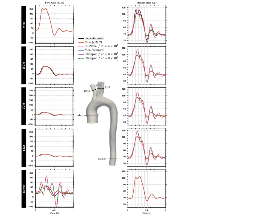
Figure 3: Comparison of experimental and simulated volumetric flow rates and pressures over time at the five caps. In both Sim-4DMRI and Sim-Idealized, in-plane motion of the wall boundary rings is enabled, and the prescribed damping constant is $c^{s}=3\times 10^{5}$ g/(cm${}^{2}\cdot$ s).

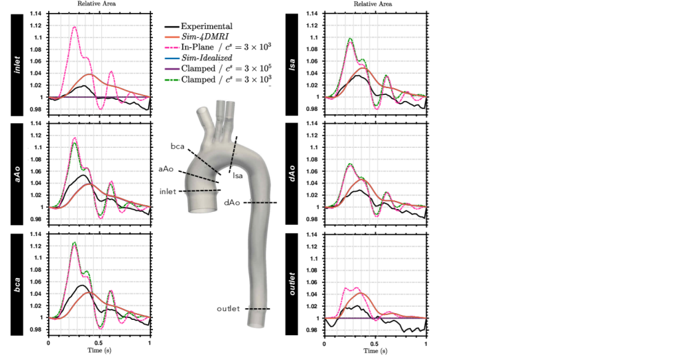
Figure 4: Comparison of experimental and simulated relative areas over time at the six 2D scan landmarks along the aortic arch. In both Sim-4DMRI and Sim-Idealized, in-plane motion of the wall boundary rings is enabled, and the prescribed damping constant is $c^{s}=3\times 10^{5}$ g/(cm${}^{2}\cdot$ s). We note that the experimentally measured areas do not exhibit periodicity, displaying a sharp jump from $t=0.98$ s to the artificially repeated $t=0.0$ value for $t=1.0$ s.

3 Results

Comparisons between simulated and experimentally measured volumetric flow rates, pressures, and relative areas over the cardiac cycle are shown in Figures 3 and 4. Whereas the experimental flow rates plotted for inlet and outlet were computed from 4D-flow velocities, those plotted for BCA, LCA, and LSA were computed from 2D cine PC-MRI velocities, given the 4D-flow MRI registration discrepancies discussed in Section 2.6.2. We focus first on Sim-4DMRI and Sim-Idealized. As expected, flow rate discrepancies from the experimental results were observed only for outlet, the only cap for which a Neumann condition was prescribed. While exact mass conservation would not be expected either experimentally or numerically, the experimental flow rates exhibited a mean loss of $5.01$ mL/s from the inflow ($77.8$ mL/s); by comparison, Sim-4DMRI and Sim-Idealized exhibited mean gains of only $0.0671$ mL/s and $0.0765$ mL/s, respectively, from the inflow ($77.8$ mL/s).

Relative to the experimental inlet pressure, the corresponding Sim-4DMRI and Sim-Idealized pressures were lower in systole and higher in diastole, suggesting larger numerical compliance. The experimental outlet pressure was numerically prescribed, and no experimental pressure measurements were available for BCA, LCA, or LSA. This increased numerical compliance, which was further supported by the larger simulated relative area changes in $4$ of the $6$ landmarks along the aortic arch, can be attributed to the adopted linear elasticity with a tangential Young’s modulus taken at the mean pressure. Closer agreement would be expected with future extensions to nonlinear models.

Turning our attention to the three supplemental simulations, we observed that the simulation with the same damping constant $c^{s}=3\times 10^{5}$ g/(cm${}^{2}\cdot$ s) as Sim-4DMRI but with clamped wall boundary rings yielded flow rates, pressures, and relative areas that were practically indistinguishable from those of Sim-4DMRI, with the exception of the constant inlet and outlet areas. On the other hand, the two simulations with the reduced $c^{s}=3\times 10^{3}$ g/(cm${}^{2}\cdot$ s) exhibited significant oscillations in all non-prescribed flow rates and pressures and all areas at non-clamped landmarks.

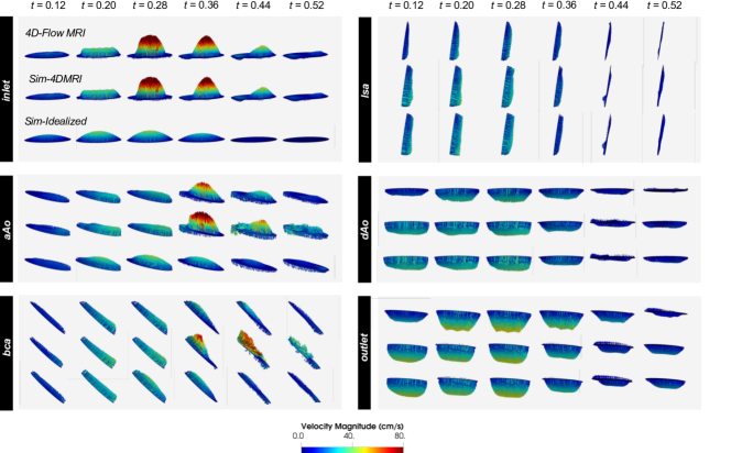
Figure 5: 4D-flow MRI (top), Sim-4DMRI (middle), and (C) Sim-Idealized (bottom) velocity profiles at $6$ evenly spaced temporal frames spanning the systolic phase of the cardiac cycle. All six 2D scan landmarks along the aortic arch are included.

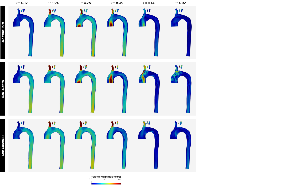
Figure 6: 4D-flow MRI (top), Sim-4DMRI (middle), and Sim-Idealized (bottom) velocity profiles on a sagittal plane at $6$ evenly spaced temporal frames spanning the systolic phase of the cardiac cycle.

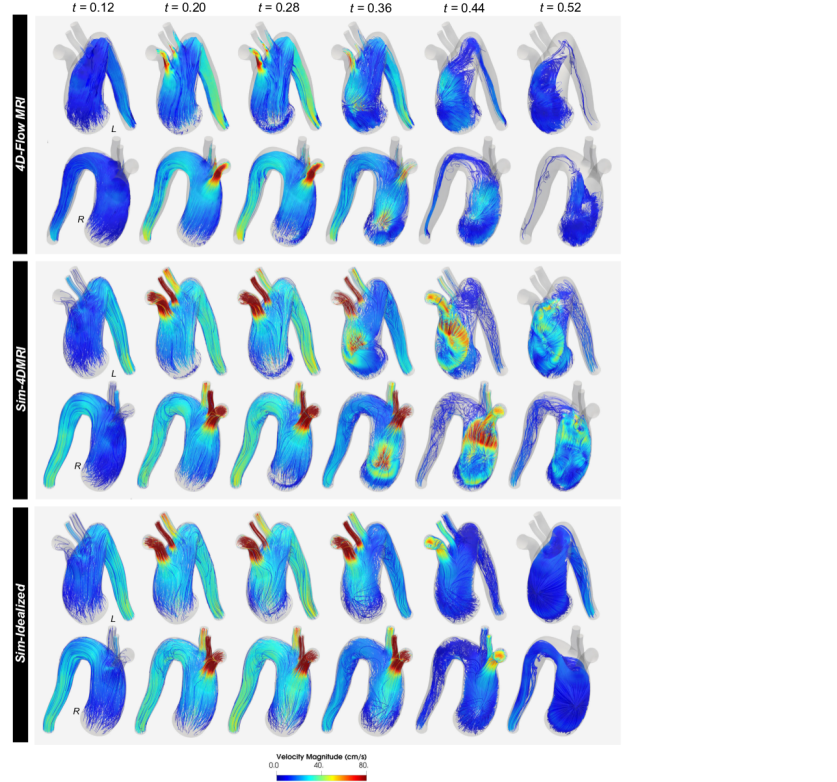
Figure 7: Streamlines computed from 4D-flow MRI (top), Sim-4DMRI (middle), and Sim-Idealized (bottom) velocities at $6$ evenly spaced temporal frames spanning the systolic phase of the cardiac cycle. The left (L, top) and right (R, bottom) lateral sides are annotated.

We investigated the experimental 4D-flow MRI and simulated velocity profiles (Figure 5) at $6$ evenly spaced temporal frames spanning systole (annotated in Figures 3 and 4), beginning with acceleration at $t=0.12$ s, peak systole from $t=0.20$ to $t=0.28$ s, and ending with deceleration from $t=0.36$ to $t=0.52$ s. All six 2D scan landmarks along the aortic arch were included. Focusing only on Sim-4DMRI, we observed close agreement in the profile shapes in all frames leading up to peak systole albeit the higher simulated velocities in the descending aorta, as expected given the higher simulated flow rates seen in Figure 3. Ascending aortic velocity magnitudes in the deceleration phase, however, revealed that the simulation captured stronger forward flow as well as stronger reverse flow along the exterior curve of the ascending aorta. These differences were similarly observed from sagittal velocity fields at the same temporal frames (Figure 6), noting again that no comparisons could be drawn for the misaligned neck arteries. Barring the higher velocity magnitudes in the descending aorta at $t=0.12$ s, our simulation almost exactly reproduced the experimental velocity fields leading up to peak systole. We also observed close agreement during fluid deceleration with regard to the shape and angle of the jet, including its curved tip near the brachiocephalic artery take-off.

To comprehend the 3D flow behavior, we turned our attention to streamlines (Figure 7). In both Sim-4DMRI and the experiment, flow near the inlet reversed along the proximal aortic wall at the onset of fluid deceleration following peak systole at $t=0.28$ s. This reversed flow continued to grow in strength until formation of a vortex at $t=0.40$ s along the left lateral wall. Despite the significantly lower velocity magnitudes in the 4D-flow data, we observed notable agreement in the vortex shape and location in the final two highlighted frames. We do, however, note the presence of three additional smaller vortices in Sim-4DMRI that were absent from the experiment: one along the right lateral wall (formed at $t=0.46$s), and two on either side of the sagittal plane (formed at $t=0.50$ s). Whereas the single vortex in the experimental data persisted until the end of the cardiac cycle, the presence of multiple interacting vortices in Sim-4DMRI caused the four initial vortex structures to progressively break up into increasing numbers of smaller vortices.

In contrast to these Sim-4DMRI results, velocity fields from Sim-Idealized failed to capture key salient features of the experimental fields, including the shape and angle of the jet. Furthermore, the ascending aortic velocity magnitudes were much too low throughout systole, the onset of flow reversal was delayed until $t=0.40$ s, and vortex formation was similarly delayed until the end of systole at $t=0.56$ s.

In computing the experimental PWV, the presence of numerous outlier TTF points yielded $698$ cm/s with an LSE regression but $578$ cm/s with a RANSAC regression. By comparison, LSE and RANSAC regressions for Sim-4DMRI yielded similar PWV estimates of $624$ cm/s and $630$ cm/s, respectively, both with equally high coefficients of determination $R^{2}$ indicating excellent fits (Figure 8). Importantly, our simulated PWV values fell within the experimental bounds.

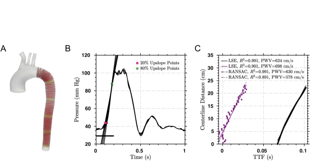
Figure 8: Numerical pulse wave velocity (PWV) computation for Sim-4DMRI using (A) $50$ equidistant normal slices along the descending aorta. (B) Simulated pressure waveforms and lines used to determine times-to-foot (TTFs) are plotted for the five representative yellow slices. (C) Experimental (purple) and numerical (black) PWV estimates determined as slopes of linear regressions, performed with either least squares error (LSE) or Random Sample Consensus (RANSAC), relating TTF to the distance along the descending aortic centerline. The time delay seen in the numerical results relative to the experimental results is a consequence of the use of pressure rather than flow waveforms.

4 Discussion

Our study represents the first to validate a cardiovascular FSI formulation against an in vitro flow circuit involving a compliant patient-specific vascular phantom. Novel aspects spanning both the experimental and numerical fronts include (i) rapid, cost-effective, and repeatable PolyJet photopolymerization of a compliant aortic model; (ii) mechanical characterization of the phantom for FSI parameter estimation; (iii) the use of multiple MRI sequences to achieve high-resolution anatomical and hemodynamic data; (iv) in-plane motion of inlet and outlet surfaces to circumvent nonphysiological clamping; (v) external tissue support to model the embedding gel block; and (vi) vascular wall prestressing to reflect imaging under experimental steady flow conditions.

When Moireau et al. [30] first proposed external tissue support, they also found it effective at eliminating rapid wall oscillations observed with CMM [7], which have long been hypothesized to arise from clamping-induced wave reflections. Nonetheless, Figures 3 and 4 clearly indicate that even with in-plane motion of $\Gamma^{i}_{\mathrm{ring}}$ nodes, viscous damping beyond some threshold level was necessary to suppress oscillations in our study. To better understand the source of these oscillations, we additionally replaced the flow rate and pressure boundary conditions at the outlets with Windkessel models; no oscillations were observed even when clamping $\Gamma^{i}_{\mathrm{ring}}$ nodes in the absence of external tissue support. Prescribing the resulting inlet, BCA, LCA, and LSA flow rates and outlet pressure from this Windkessel simulation in a subsequent simulation also produced no oscillations. Together, these observations suggested that the oscillations requiring damping in our study were driven by the assignment of experimental waveforms.

Despite discrepancies in the velocity fields during deceleration, our simulation captured key salient features of the 4D-flow MRI data, including the (i) region and trajectory of reverse flow following peak systole, (ii) shape and angle of the jet, and (iii) shape and location of the primary vortex. On the other hand, Sim-Idealized exhibited poor agreement with the 4D-flow MRI data in numerous aspects including the ascending aortic velocity magnitudes, shape and angle of the jet, duration of flow reversal, and time of vortex formation. These discrepancies highlight the importance of assigning non-idealized inlet velocity profiles.

Previous in vitro and in vivo validation studies [19, 4, 32] have similarly reported larger velocity field discrepancies during deceleration, with simulations exhibiting complex secondary flow features that were absent from the 4D-flow MRI data. These discrepancies in complex flow structures can partially be explained by the many issues inherent to 4D-flow MRI. In particular, despite the many corrections applied to the acquired velocity fields either during or following image reconstruction to reduce phase offsets, the resulting 4D-flow MRI velocity fields are not completely divergence-free, signaling a lack of conservation of mass. Solenoidal filtering and related divergence-free methods [33] could be explored in the future. Furthermore, image acquisition in k-space over extended durations of time yields images that are temporally averaged over tens of cardiac cycles, and furthermore averaged within each temporal bin corresponding to the temporal resolution ($0.02$ s here). Boundary voxels capturing both the fluid and surrounding wall are also subject to the partial volume effect [9]. The combined effect of partial voluming and temporal averaging over a deforming domain presents challenges for deriving accurate boundary conditions reflective of the in vivo or in vitro conditions to be prescribed in simulations. Additional sources of error existed in our study, as indicated by the lack of conservation of mass, absence of periodicity in luminal areas, and the large number of outliers yielding regression-dependent PWV estimates. Moreover, the misalignment of the neck arteries hindered our ability to assign non-idealized velocity profiles at the corresponding BCA, LCA, and LSA outlets. The resulting parabolic profiles and limited unidirectional velocity encoding of 2D cine PC-MRI likely introduced discrepancies that were propagated into the flow domain.

Overall, close agreement in pressures, lumen area changes, pulse wave velocity, early systolic velocities, and late systolic flow structures validates our numerical methodology, including the RUC formulation, in-plane deformation at model inlets and outlets, viscoelastic external tissue support, and vascular tissue prestressing. Together, our suite of computationally efficient FSI techniques offers a platform for investigating vascular disease initiation, progression, and treatment.

References

- [1] J. Alastruey. Numerical modelling of pulse wave propagation in the cardiovascular system: development, validation and clinical applications. PhD thesis, Imperial College London, 2006.
- [2] G. Annio, R. Torii, A. Ducci, V. Muthurangu, V. Tsang, and G. Burriesci. Experimental Validation of Enhanced Magnetic Resonance Imaging (EMRI) Using Particle Image Velocimetry (PIV). Annals of Biomedical Engineering, 49:3481–3493, 2021.
- [3] Y. Bazilevs, M.-C. Hsu, Y. Zhang, W. Wang, T. Kvamsdal, S. Hentschel, and J. Isaksen. Computational vascular fluid-structure interaction: methodology and application to cerebral aneurysms. Biomechanics and Modeling in Mechanobiology, 9(4):481–498, 2010.
- [4] G. Biglino, D. Cosentino, J. Steeden, L. De Nova, M. Castelli, H. Ntsinjana, G. Pennati, A. Taylor, and S. Schievano. Using 4D Cardiovascular Magnetic Resonance Imaging to Validate Computational Fluid Dynamics: A Case Study. Frontiers in Pediatrics, 3:107, 2015.
- [5] G. Biglino, P. Verschueren, R. Zegels, A. Taylor, and S. Schievano. Rapid prototyping compliant arterial phantoms for in-vitro studies and device testing. Journal of Cardiovascular Magnetic Resonance, 15:2, 2013.
- [6] Z. Cheng, C. Juli, N. Wood, R. Gibbs, and X. Xu. Predicting flow in aortic dissection: comparison of computational model with PC-MRI velocity measurements. Medical Engineering & Physics, 36(9):1176–1184, 2014.
- [7] C. Figueroa, I. Vignon-Clementel, K. Jansen, T. Hughes, and C. Taylor. A coupled momentum method for modeling blood flow in three-dimensional deformable arteries. Computer Methods in Applied Mechanics and Engineering, 195:5685–5706, 2006.
- [8] J. Fonken, E. Maas, A. Nievergeld, M. van Sambeek, F. van de Vosse, and R. Lopata. Ultrasound-Based Fluid-Structure Interaction Modeling of Abdominal Aortic Aneurysms Incorporating Pre-stress. Frontiers in Physiology, 12:1255, 2021.
- [9] M. González Ballester, A. Zisserman, and M. Brady. Estimation of the partial volume effect in MRI. Medical Image Analysis, 6(4):389–405, 2000.
- [10] D. Griffiths. Treatment of skew boundary conditions in finite element analysis. Computers & Structures, 36(6):1009–1012, 1990.
- [11] W. Ho, I. Tshimanga, M. Ngoepe, M. Jermy, and P. Geoghegan. Evaluation of a desktop 3D Printed Rigid Refractive-Indexed-Matched Flow Phantom for PIV Measurements on Cerebral Aneurysms. Cardiovascular Engineering and Technology, 11(1):14–23, 2020.
- [12] M.-C. Hsu and Y. Bazilevs. Blood vessel tissue prestress modeling for vascular fluid–structure interaction simulation. Finite Elements in Analysis and Design, 47(6):593–599, 2011.
- [13] C. Ionita, M. Mokin, N. Varble, D. Bednarek, J. Xiang, K. Snyde, A. Siddiqui, E. Levy, H. Meng, and S. Rudin. Challenges and limitations of patient-specific vascular phantom fabrication using 3D Polyjet printing. Proceedings of SPIE - The International Society for Optical Engineering, 9038:90380M, 2014.
- [14] A. Kaiser, N. Schiavone, J. Eaton, and A. Marsden. Validation of Immersed Boundary Simulations of Heart Valve Hemodynamics against In Vitro 4D Flow MRI Data. arXiv:2111.00720 [q-bio.TO], 2021.
- [15] P. Knoops, G. Biglino, A. Hughes, K. Parker, L. Xu, S. Schievano, and R. Torii. A Mock Circulatory System Incorporating a Compliant 3D-Printed Anatomical Model to Investigate Pulmonary Hemodynamics. Artificial Organs, 41(7):637–646, 2017.
- [16] C. Kolyva, G. Biglino, J. Pepper, and A. Khir. A mock circulatory system with physiological distribution of terminal resistance and compliance: application for testing the intra-aortic balloon pump. Artificial Organs, 36(3):E62–70, 2012.
- [17] J. Ku, M. Draney, F. Arko, W. Lee, F. Chan, N. Pelc, C. Zarins, and C. Taylor. In vivo validation of numerical prediction of blood flow in arterial bypass grafts. Annals of Biomedical Engineering, 30(6):743–752, 2002.
- [18] E. Kung, A. Les, C. Figueroa, F. Medina, K. Arcaute, R. Wicker, M. McConnell, and C. Taylor. In vitro validation of finite element analysis of blood flow in deformable models. Annals of Biomedical Engineering, 39:1947–1960, 2011.
- [19] E. Kung, A. Les, F. Medina, R. Wicker, M. McConnell, and C. Taylor. In vitro validation of finite-element model of AAA hemodynamics incorporating realistic outlet boundary conditions. Journal of Biomechanical Engineering, 133(4):041003, 2011.
- [20] H. Lan, A. Updegrove, N. Wilson, G. Maher, S. Shadden, and A. Marsden. A Re-Engineered Software Interface and Workflow for the Open-Source SimVascular Cardiovascular Modeling Package. Journal of Biomechanical Engineering, 140(2):0245011–02450111, 2018.
- [21] I. Lan, J. Liu, W. Yang, and A. Marsden. A reduced unified continuum formulation for vascular fluid-structure interaction. arXiv:2110.08391 [physics.comp-ph], 2021.
- [22] I. Lan, J. Liu, W. Yang, and A. Marsden. Numerical investigation of abdominal aortic aneurysm hemodynamics using the reduced unified continuum formulation for vascular fluid-structure interaction. arXiv:2201.04016 [physics.med-ph], 2022.
- [23] J. Liu, I. Lan, O. Tikenogullari, and A. Marsden. A note on the accuracy of the generalized- scheme for the incompressible Navier-Stokes equations. International Journal for Numerical Methods in Engineering, 122:638–651, 2021.
- [24] J. Liu, M. Latorre, and A. Marsden. A continuum and computational framework for viscoelastodynamics: I. finite deformation linear models. Computer Methods in Applied Mechanics and Engineering, 385:114059, 2021.
- [25] J. Liu and A. Marsden. A unified continuum and variational multiscale formulation for fluids, solids, and fluid–structure interaction. Computer Methods in Applied Mechanics and Engineering, 337:549–597, 2018.
- [26] J. Liu, A. Marsden, and Z. Tao. An energy-stable mixed formulation for isogeometric analysis of incompressible hyperelastodynamics. International Journal for Numerical Methods in Engineering, 120:937–963, 2019.
- [27] J. Liu, W. Yang, M. Dong, and A. Marsden. The nested block preconditioning technique for the incompressible Navier-Stokes equations with emphasis on hemodynamic simulations. Computer Methods in Applied Mechanics and Engineering, 367:113122, 2020.
- [28] Q. Long, X. Xu, B. Ariff, S. Thom, A. Hughes, and A. Stanton. Reconstruction of blood flow patterns in a human carotid bifurcation: A combined CFD and MRI study. Journal of Magnetic Resonance Imaging, 11(3):299–311, 2000.
- [29] M. Markl, W. Wallis, S. Brendecke, J. Simon, A. Frydrychowicz, and A. Harloff. Estimation of global aortic pulse wave velocity by flow-sensitive 4D MRI. Magnetic Resonance in Medicine, 63(6):1575–1582, 2010.
- [30] P. Moireau, N. Xiao, M. Astorino, C. Figueroa, D. Chapelle, C. Taylor, and J. Gerbeau. External tissue support and fluid–structure simulation in blood flows. Biomechanics and Modeling in Mechanobiology, 11:1–18, 2012.
- [31] R. Pons, A. Guala, J. Rodríguez-Palomares, J. Cajas, L. Dux-Santoy, G. Teixidó-Tura, J. Molins, M. Vázquez, A. Evangelista, and J. Martorell. Fluid-structure interaction simulations outperform computational fluid dynamics in the description of thoracic aorta haemodynamics and in the differentiation of progressive dilation in Marfan syndrome patients. Royal Society Open Science, 7(2):191752, 2020.
- [32] S. Saitta, S. Pirola, F. Piatti, E. Votta, F. Lucherini, F. Pluchinotta, M. Carminati, M. Lombardi, C. Geppert, F. Cuomo, C. Figueroa, X. Xu, and A. Redaelli. Evaluation of 4D flow MRI-based non-invasive pressure assessment in aortic coarctations. Journal of Biomechanics, 94:13–21, 2019.
- [33] D. Schiavazzi, F. Coletti, G. Iaccarino, and J. Eaton. A matching pursuit approach to solenoidal filtering of three-dimensional velocity measurements. Journal of Computational Physics, 263(C):206–221, 2014.
- [34] D. Tanné, E. Bertrand, L. Kadem, P. Pibarot, and R. Rieu. Assessment of left heart and pulmonary circulation flow dynamics by a new pulsed mock circulatory system. Experiments in Fluids, 48:837–850, 2010.
- [35] J. Zhou, M. Esmaily-Moghadam, T. Conover, T.-Y. Hsia, A. Marsden, R. Figliola, and The MOCHA Investigators. In Vitro Assessment of the Assisted Bidirectional Glenn Procedure for Stage One Single Ventricle Repair. Cardiovascular Engineering and Technology, 6(3):256–267, 2015.
- [36] J. Zimmermann, M. Loecher, F. Kolawole, K. Bäumler, K. Gifford, S. Dual, M. Levenston, A. Marsden, and D. Ennis. On the impact of vessel wall stiffness on quantitative flow dynamics in a synthetic model of the thoracic aorta. Scientific Reports, 11(1):6703, 2021.