CHEMOUT: CHEMical complexity in star-forming regions of the OUTer Galaxy. I. Organic molecules and tracers of star-formation activity

Abstract

Context. The outer Galaxy is an environment with metallicity lower than the Solar one. Because of this, the formation and survival of molecules in star-forming regions located in the inner and outer Galaxy is expected to be different.

Aims. To gain understanding on how chemistry changes throughout the Milky Way, it is crucial to observe outer Galaxy star-forming regions to constrain models adapted for lower metallicity environments.

Methods. In this paper we present a new observational project: chemical complexity in star-forming regions of the outer Galaxy (CHEMOUT). The goal is to unveil the chemical composition in 35 dense molecular clouds associated with star-forming regions of the outer Galaxy through observations obtained with the IRAM 30m telescope in specific 3mm and 2mm spectral windows.

Results. In this first paper, we present the sample, and report the detection at 3 mm of simple organic species HCO⁺, H¹³CO⁺, HCN, c-C₃H₂, HCO, C₄H, and HCS⁺, of the complex hydrocarbon CH₃CCH, and of SiO, CCS and SO. From the optically thin line $J_{K_{a},K_{b}}=2_{1,2}-1_{0,1}$ of c-C₃H₂  we estimate new kinematic heliocentric and Galactocentric distances based on an updated rotation curve of the Galaxy. The detection of the molecular tracers does not seem to have a clear dependence on the Galactocentric distance. Moreover, with the purpose of investigating the occurrence of outflows and investigate the association with protostellar activity, we analyse the HCO⁺ line profiles. We find high velocity wings in $\sim 71\%$ of the targets, and their occurrence does not depend on the Galactocentric distance.

Conclusions. Our results, confirmed by a statistical analysis, show that the presence of organic molecules and tracers of protostellar activity is ubiquitous in the low-metallicity environment of the outer Galaxy. Based on this, and on the additional evidence that small, terrestrial planets are omnipresent in the Galaxy, we support previous claims that the definition of Galactic Habitable Zone should be rediscussed in view of the ubiquitous capacity of the interstellar medium to form organic molecules.

1 Introduction

Table 1: Source parameters extracted from Table 1 of Blair et al. (2008).

source	R.A.	Dec.	$V_{\rm LSR}$(1)	$N(H_{2})$(2)	$R^{old}_{\rm GC}$(3)	$M$(4)	$L$(4)
	(J2000)	(J2000)	km s-1	$\times 10^{21}$cm-2	kpc	M⊙	($\times 10^{3}$) L⊙
WB89-315	00:05:53.8	64:05:17	–95.09	3.7	17.1
WB89-379	01:06:59.9	65:20:51	–89.32	6.5	17.3	532	1.44
WB89-380	01:07:50.9	65:21:22	–86.67	11.4	17.0
WB89-391	01:19:27.1	65:45:44	–86.06	5.2	16.9
WB89-399	01:45:39.4	64:16:00	–82.19	6.3	16.8	1685	16.3
WB89-437	02:43:29.0	62:57:08	–71.72	14.2	16.2
WB89-440	02:46:07.3	62:46:31	–72.20	4.1	16.4
WB89-501	03:52:27.6	57:48:34	–58.44	11.2	16.4
WB89-529	04:06:25.5	53:21:49	–60.08	4.7	17.8	408	10.1
WB89-572	04:35:58.3	47:42:58	–48.03	3.8	20.4
WB89-621	05:17:13.4	39:22:15	–25.38	13.0	22.6	920	41.2
WB89-640	05:25:40.7	41:41:53	–25.42	3.2	18.4
WB89-670	05:37:41.9	36:07:22	–17.52	7.3	23.5
WB89-705	05:47:47.6	35:22:01	–12.10	1.7	21.4
WB89-789	06:17:24.3	14:54:37	34.33	5.8	20.3	1066	9.75
WB89-793	06:18:41.7	15:04:52	30.48	5.9	18.1	204	0.77
WB89-898	06:50:37.3	$-$05:21:01	63.41	2.5	16.4
19383+2711	19:40:22.1	27:18:33	–66.85	–	13.2
19423+2541	19:44:23.2	25:48:40	–72.62	–	13.6	1278	104.5
19489+3030	19:50:53.2	30:38:09	–68.91	–	13.0
19571+3113	19:59:08.5	31:21:47	–62.48	–	12.2
20243+3853	20:26:10.8	39:03:30	–73.06	–	12.9	891	15.9
WB89-002	20:37:22.3	47:13:54	–2.75	7.8	8.6
WB89-006	20:42:58.2	47:35:35	–91.38	6.3	14.9
WB89-014	20:52:07.8	49:51:28	–96.03	4.6	15.5
WB89-031	21:04:18.0	46:53:10	–89.40	1.2	14.6
WB89-035	21:05:19.7	49:15:59	–77.68	5.2	13.4	367	5.23
WB89-040	21:06:50.0	50:02:09	–62.65	4.1	12.1	613	0.62
WB89-060	21:15:56.0	54:43:33	–84.29	9.3	14.0
WB89-076	21:24:29.0	53:45:35	–97.17	5.0	15.7	355	0.82
WB89-080	21:26:29.1	53:44:11	–74.24	8.5	13.1	299	1.44
WB89-083	21:27:47.7	54:26:58	–93.77	2.8	15.3	220	0.82
WB89-152	22:05:15.4	60:48:41	–88.13	2.8	14.8
WB89-283	23:32:23.8	63:33:18	–94.49	5.8	16.5	140	4.80
WB89-288	23:36:08.1	62:23:48	–100.87	3.4	17.5	373	3.22

⁽¹⁾ Local Standard of Rest velocities used to centre the spectra;
⁽²⁾ H₂ column densities from CO (1–0) (Blair et al. 2008), assuming a standard CO-H₂ conversion factor of 1.8$\times 10^{20}$ cm^-2 (K Km s^-1)^-1 (Dame et al. 2001) valid at the Solar Circle. The values are averaged within the Arizona Radio Observatory (ARO) main beam of 44^′′;
⁽³⁾ Galactocentric distances based on the rotation curve of Brand & Blitz (1993). We will derive updated $R_{\rm GC}$ in Sect. 4.3;
⁽⁴⁾ total gas mass, $M$, and bolometric luminosity, $L$, respectively, derived from Herschel measurements by Elia et al. (2021), and rescaled when needed to the new heliocentric distances calculated in this work (Table 6).

The outer Galaxy (OG) is the portion of the Galactic disk located at Galactocentric distances, $R_{\rm GC}$, in between $9\leq R_{\rm GC}\leq 24$ kpc, i.e. beyond the Solar Circle. It shows chemical properties significantly different from those of the inner Galaxy. In particular, the overall metallicity is lower than the Solar one (e.g., a factor of four lower at $R_{\rm GC}=19$ kpc, Shimonishi et al. 2021). The elemental abundances of oxygen, carbon, and nitrogen, i.e. the three most abundant elements in the Universe after hydrogen and helium, decrease as a function of $R_{\rm GC}$ (see e.g. Esteban et al. 2017), as all the other elements, following the so-called radial metallicity gradient. Despite the fact that the OG is believed to be more favourable than the inner Galaxy for preserving life on habitable planets, due to the low rate of disruptive events (e.g. Piran & Jiménez et al. 2014; Vukotić et al. 2016), the lower abundance of heavy elements with respect to the Solar one has suggested in the past that this zone is not suitable to form planetary systems in which Earth-like planets could be born and might be capable of sustaining life (Prantzos 2008, Ramírez et al. 2010). Chemical evolution models predict that the so-called Galactic Habitable Zone (GHZ) in the Milky Way is an annulus extended up to $R_{\rm GC}\sim 9$ kpc, with maximum habitability at $R_{\rm GC}\sim 8$ kpc (Spitoni et al. 2014, 2017).

However, this scenario has been challenged by recent observational results, in which the occurrence of Earth-like planets does not seem to depend on the Galactocentric distance (e.g. Maliuk & Budaj 2020). The formation of small, terrestrial planets does not require a metal-rich environment, suggesting that their existence might be widespread in the disk of the Galaxy (Mulders 2018). In addition, the mass of Super-Earths and Sub-Neptunes planets is not determined by the availability of solids, but is instead regulated by poorly known processes, with a very weak dependence on metallicity (Kutra et al. 2021, Pacetti et al. 2020).

All this indicates that, even at metallicities lower than the Solar one, planets capable to host life can be found. Moreover, recent observations performed with the Atacama Large Millimeter Array (ALMA) of the Large and Small Magellanic Clouds (LMC and SMC, respectively), which have a metallicity of a factor  3 and  5 lower, respectively, than the Solar one, have revealed emission of complex organic molecules (COMs), i.e. organic species with more than 5 atoms. Methanol, CH₃OH, was detected in star-forming regions associated with both galaxies (Shimonishi et al. 2018; Sewiło et al. 2018), and methyl formate (HCOOCH₃) and dimethyl ether (CH₃OCH₃) were found in hot-cores of the LMC (Sewiło et al. 2018). Because these COMs are thought to be precursors of more complex biogenic molecules (see e.g. Caselli & Ceccarelli 2012), these observational findings indicate that the basic bricks of organic chemistry can be found also in metal poor environments. These findings were reinforced by the recent detections of a hot molecular core, WB89-789, rich in COMs, in the extreme OG (Shimonishi et al. 2021), and of methanol in star-forming regions located at $R_{\rm GC}$ up to $\sim 23.5$ kpc (Bernal et al. 2021).

Despite these recent findings, the formation and survival of molecules in star-forming regions located in the two environments (i.e. inner and outer Galaxy) is expected to be different. In fact, besides a lower initial abundance of heavy elements in the OG, relative ratios of different elements change as well because their abudances do not vary in the same way as a function of $R_{\rm GC}$ (Esteban et al. 2017). For example, the N/O ratio has a clear negative trend with $R_{\rm GC}$ (Magrini et al. 2018). Moreover, Berg et al. (2016) suggest for the C/O ratio a flat relation at metallicity lower than the Solar one, and a steeply increasing slope at higher metallicities, i.e. with decreasing $R_{\rm GC}$, even though different trends are found at low metallicities from state-of-the-art analysis of high-resolution spectra of solar neighbourhood halo dwarf stars (e.g. Amarsi et al. 2019). Both parameters, i.e. the initial elemental abundances and their relative ratios, are crucial inputs of chemical models that attempt to reproduce the observed molecular emission in star-forming regions (e.g. star-forming cores, Fontani et al. 2017; protoplanetary disks, Eistrup et al. 2018; extragalactic environments, Sewiło et al. 2018). Therefore, to gain understanding on how chemistry changes throughout the Galaxy and constrain models adapted for lower metallicity environments, it is crucial to observe OG star-forming regions in a large variety of molecular tracers.

With the aim of attacking this problem, we have started the observational project called ’CHEMical complexity in star-forming regions of the OUTer Galaxy’ (CHEMOUT). The immediate goal, based on observations with the IRAM 30m telescope, is to unveil the chemical composition in star-forming regions of the OG. Thanks to these observations, we will start to investigate how molecules form in such low-metallicity environment. In particular, molecules that are potentially biogenic species, such as COMs, carbon chains, and sulfur- and phosphorus-bearing molecules, are of particular interest since in star-forming cloud cores they are expected to be part of the planetesimals out of which planets form and/or can be delivered to the surfaces of planets, where they might play key roles in the origin of life. For this reason, the results of CHEMOUT will also allow us to prepare the ground for a re-discussion of the concept of GHZ. Moreover, the isotopic abundances and abundance ratios determined by CHEMOUT will be used to constrain Galactic chemical evolution and stellar nucleosynthesis models at low metallicities. CHEMOUT data will be especially useful to study the evolution of rare isotopes that lack spectroscopic determinations in stellar atmospheres - such as, for instance, ¹⁵N - or for which statistically relevant stellar samples are not in hand at present (e.g., ¹³C, ¹⁷O, and ¹⁸O).

In this first paper, we present the list of targets (Sect. 2), the first observational dataset (Sect. 3), and show as first results the detection of several organic species and tracers of star-formation activity (such as SO and SiO). These results are shown and described in Sect. 4, and discussed in Sect. 5. The main conclusions and the outlook of the project are given in Sect. 6.

2 Sample

Table 2: Spectral windows observed and observational parameters

Spectral	HPBW	$V_{\rm res}$(a)	$\eta_{\rm MB}$(b)
windows
(GHz)	(′′)	(km s-1)
85.310 - 87.130	28	$\sim 0.16$	0.85
88.590 - 90.410	27	$\sim 0.16$	0.84
151.750 - 153.570	15	$\sim 0.096$	0.77
148.470 - 150.290	15	$\sim 0.096$	0.77

^(a) velocity resolution in the spectrum;
^(b) defined as $\eta_{\rm MB}=B_{\rm eff}/F_{\rm eff}$, where $B_{\rm eff}$ is the main beam efficiency and $F_{\rm eff}$ the forward efficiency.

We have observed 35 targets extracted from Blair et al. (2008), who searched for formaldehyde emission with the Arizona Radio Observatory (ARO) 12m telescope in dense molecular cloud cores of the OG associated with IRAS colours typical of star-forming regions. The list of targets is given in Table 1. We selected objects (1) clearly detected in H₂CO $J_{K_{a},K_{b}}=2_{1,2}-1_{1,1}$, and (2) covering as much as possible the full range of $R_{\rm GC}$ in the OG. The targets have $R_{\rm GC}$ in between $\sim 9$ and $\sim 24$ kpc from the Galactic Centre. Table 1 shows the target equatorial (J2000) coordinates. In the same Table we also report two parameters taken from Blair et al. (2008), namely the H₂ total column density, N(H₂), and the Galactocentric distance, $R^{old}_{\rm GC}$. In Sect. 4.3 we will recompute $R_{\rm GC}$, $R^{new}_{\rm GC}$, based on the systemic velocity of the sources derived from our new data, and using an updated rotation curve of the Galaxy. For the objects included in the Hi-GAL catalogs (Molinari et al. 2016), in Table 1 we also give the total gas mass ($M$) and bolometric luminosity ($L$) derived from Herschel observations (Elia et al. 2021) and rescaled for the new heliocentric distances calculated in this work (Sect. 4.3).

The masses listed in Table 1 indicate that about half of the targets are candidate high-mass star-forming regions. Because the sources for which the mass has not been estimated yet have comparable distances and intensities of the H₂CO lines (Blair et al. 2008), it is expected that all objects have similar physical properties, and hence they are all good candidate high-mass star-forming regions. However, only accurate measurements of their gas masses will allow to confirm (or deny) this hypothesis. The location of the sources in the Galactic plane is illustrated in Fig. 1. Most of the sources are included in the II quadrant of the Galaxy. WB89-002, the only object in Blair et al. (2008) located very close to the Sun ($R_{\rm GC}\sim 8.6$ kpc), was included in this study to have at least one target representative of the Sun neighbourhoods observed with exactly the same observational setup as the OG sources. This will allow us to derive observational trends or gradients (e.g. abundance gradients or isotopic fraction gradients) from the OG to the Sun location without extrapolating.

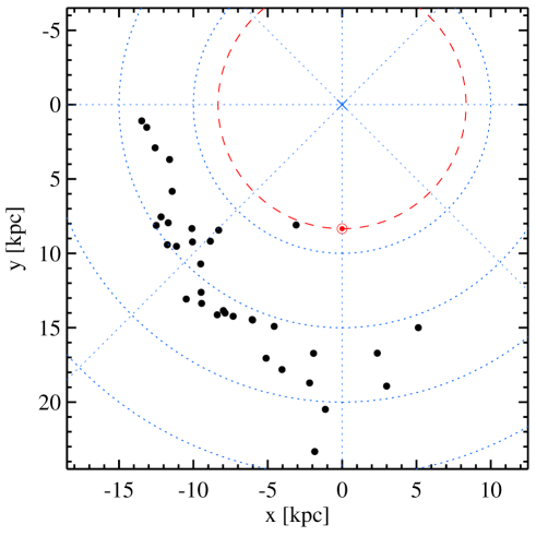
Figure 1: Plan view of the Galactic disk showing the location of the sources in Table 1 (filled points) after recalculating their Galactocentric and heliocentric distances (Sect. 4.3). The Sun is marked by the red-circled point, and the Galactic centre is pinpointed by the blue cross. The Solar circle is shown by the red dashed curve. The blue dotted circles correspond to Galactocentric distances of 10, 15, 20, and 25 kpc.

3 Observations

Table 3: Molecular lines of species detected in the spectral windows at 3 mm listed in Table 2 at a significance level well above 3$\sigma$ rms (Y) or comparable to 3$\sigma$ rms (Y?).

source	rms(1)	carbon-bearing species										other species(3)
	(mK)
		c-C3H2	HCS+	CH3CCH	C4H	CCS	HCO	H13CO+	HCN	HCO+(2)		NH2D	SO	SiO
WB89-315	$\sim 9.1$	n	n	n	n	n	n	n	Y	Y(n)		n	n	n
WB89-379	$\sim 6.0$	Y	Y	Y	n	n	Y	Y	Y	Y(y?)		n	Y	Y?
WB89-380	$\sim 17$	Y	n	Y?	n	n	Y	Y	Y	Y(2,y)		n	Y	Y
WB89-391	$\sim 6.6$	Y	Y?	n	n	n	Y	Y	Y	Y(y?)		n	Y	Y
WB89-399	$\sim 9.3$	Y	n	n	Y?	n	Y	Y?	Y	Y(y?)		n	n	Y?
WB89-437	$\sim 6.0$	Y	Y	Y	Y	Y?	Y	Y	Y	Y(y)		Y	Y	Y
WB89-440	$\sim 6.7$	Y	n	n	n	n	Y	n	Y	Y(n)		n	n	Y
WB89-501	$\sim 7.2$	Y	n	n	n	n	Y	Y	Y	Y(y?)		n	Y	Y
WB89-529	$\sim 11.5$	Y	n	n	n	n	Y	n	Y	Y(n)		n	n	n
WB89-572	$\sim 26$	Y	n	n	n	n	n	Y?	Y	Y(y)		n	Y	n
WB89-621	$\sim 5.7$	Y	Y	Y	n	Y?	Y	Y	Y	Y(y)		n	Y	Y
WB89-640	$\sim 10.7$	Y	Y?	n	n	n	Y	Y	Y	Y(y)		Y	Y	n
WB89-670	$\sim 9.2$	Y	n	n	Y	Y	n	Y	Y	Y(y)		n	n	n
WB89-705	$\sim 7.8$	Y	n	n	n	n	Y?	Y	Y	Y(n)		Y	Y	n
WB89-789	$\sim 7.2$	Y	Y	Y?	n	n	Y	Y	Y	Y(y)		Y	Y	n
WB89-793	$\sim 13.2$	Y	n	n	n	n	n	Y	Y	Y(y)		n	Y	n
WB89-898	$\sim 8.4$	Y	n	n	n	n	Y?	n	Y	Y(y?)		n	Y	n
19383+2711	$\sim 6.6$	Y	Y	n	Y	n	Y	Y	Y	Y(2,n)		n	Y	Y
19423+2541	$\sim 7.6$	Y	n	n	Y?	n	Y	Y	Y	Y(y)		Y?	Y	Y
19489+3030	$\sim 6.5$	Y	Y?	n	n	n	n	Y	Y	Y(y)		Y	Y?	Y?
19571+3113	$\sim 6.0$	Y	Y?	n	n	n	Y	Y	Y	Y(2,n)		n	n	Y
20243+3853	$\sim 5.0$	Y	Y	n	Y?	n	Y	Y	Y	Y(y?)		n	Y	Y
WB89-002	$\sim 14$	Y	n	n	n	n	Y	Y?	Y	Y(n)		n	n	n
WB89-006	$\sim 7.3$	Y	Y	n	Y	n	Y?	Y	Y	Y(2,y)		Y	Y	n
WB89-014	$\sim 8.5$	Y	n	n	n	n	n	n	Y	Y(n)		n	n	n
WB89-031	$\sim 6.5$	Y	n	n	n	n	Y	n	Y	Y(y?)		n	n	Y?
WB89-035	$\sim 7.3$	Y	n	n	n	n	Y	Y	Y	Y(y)		n	Y	Y
WB89-040	$\sim 6.2$	Y	Y	n	Y?	n	Y	Y	Y	Y(y?)		n	Y	n
WB89-060	$\sim 7.1$	Y	Y	Y	n	n	n	Y	Y	Y(2,y)		n	Y	Y
WB89-076	$\sim 7.5$	Y	Y	n	Y	Y	Y	Y	Y	Y(y)		Y	Y	n
WB89-080	$\sim 8.3$	Y	n	n	n	n	Y	Y	Y	Y(2,y)		n	Y	n
WB89-083	$\sim 20$	Y	n	n	n	n	n	Y	Y	Y(n)		n	n	n
WB89-152	$\sim 14$	Y	n	n	n	n	n	n	Y	Y(n)		n	n	n
WB89-283	$\sim 7.5$	Y	n	n	n	n	Y	Y	Y	Y(y)		n	Y?	n
WB89-288	$\sim 7.4$	Y	n	n	n	n	Y	n	Y	Y(y?)		n	n	n

⁽¹⁾ 1$\sigma$ rms noise at 3 mm, calculated for a velocity resolution of $\sim 0.65$ km s^-1;
⁽²⁾ HCO⁺ $J=1-0$ line profile can show two velocity features (2), and/or high velocity wings (y/n);
⁽³⁾ We do not report the detections in the D, ¹³C and ¹⁵N isotopologues of HCN and HNC, which will be published in forthcoming papers (Colzi et al. in prep.; Fontani et al. in prep.).

The observations were performed with the IRAM 30m telescope in several observing runs (5 days in March and April, 2018, for a total of $\sim 20$ hours; August 14-21, 2018 for additional $\sim 70$ hours). In all runs we used the 3mm and 2mm receivers simultaneously. At 3 mm, the spectral windows were optimised to observe the $J=1-0$ transitions of the four less abundant isotopologues of HCN and HNC, namely H¹⁵NC, HN¹³C, H¹³CN, and HC¹⁵N. At 2 mm, we centred the bands on the DNC $J=2-1$ line. All these transitions will be analysed in forthcoming papers (Colzi et al., in prep.; Fontani et al., in prep.). The Local Standard of Rest (LSR) velocities used to centre the receiver bands are listed in Table 1. Table 2 shows the spectral ranges observed in the two receivers, as well as some technical details of the observations: the beam full width at half maximum (HPBW), the velocity resolution ($V_{\rm res}$), and the telescope efficiency ($\eta_{\rm MB}$) used to convert the spectra from antenna temperature to main beam temperature units. The observations were made in wobbler-switching mode with a wobbler throw of 240^′′. Pointing was checked (almost) every hour on nearby quasars, planets, or bright HII regions. Focus was checked on planets at the start of observations, and after sunset and sunrise. The data were calibrated with the chopper wheel technique (see Kutner & Ulich 1981), with a calibration uncertainty of about $10\%$. The spectra were obtained with the fast Fourier transform spectrometers with the finest spectral resolution (FTS50), providing a channel width of 50 kHz. In this work, the calibrated spectra were fitted with the class package of the gildas software using standard procedures. The spectral 1$\sigma$ rms noise, strongly source-dependent, is given in Table 3, and goes generally from $\sim 5$ to $\sim 26$ mK in the 3 mm band. The 2 mm band, not presented in this work, will be shown in a forthcoming paper discussing DNC emission (Fontani et al., in prep.).

4 Results

Table 4: Rest frequencies and other spectroscopic parameters of the detected molecular transitions.

molecule	rest	quantum	$E_{\rm u}$	Log[$A_{i,j}$/s]
	frequency	numbers
	MHz		K
c-C3H2	85338.89	$J_{K_{a},K_{b}}=2_{1,2}-1_{0,1}$	6.4	–4.6341
HCS+	85347.89	$J=2-1$	6.1	–4.9548
CH3CCH	85457.30	$J(K)=5(0)-4(0)$	12.3	–6.20908
	85455.67	$J(K)=5(1)-4(1)$	19.5	–6.2268
C4H	85634.00	$N=9-8$, $J=19/2-17/2$, $F=9-8$	20.5	–4.8189
	85634.02	$N=9-8$, $J=19/2-17/2$, $F=10-9$	20.5	–4.8163
	85672.58	$N=9-8$, $J=17/2-15/2$, $F=8-7$	20.6	–4.8217
	85672.58	$N=9-8$, $J=17/2-15/2$, $F=9-8$	20.6	–4.8184
NH2D	85926.28	$J_{K_{a},K_{b}}=1_{1,1}-1_{0,1}$	20.7	–5.1057
CCS	86181.39	$N=7-6$, $J=6-5$	23.3	–4.5563
SO	86093.95	$N=2-1$, $J=2-1$	19.3	–5.2799
HCO	86670.76	$N_{K_{a},K_{b}}=1_{0,1}-0_{0,0}$, $J=3/2-1/2$, $F=2-1$	4.2	–5.3289
	86708.36	$N_{K_{a},K_{b}}=1_{0,1}-0_{0,0}$, $J=3/2-1/2$, $F=1-0$	4.2	–5.3377
	86777.46	$N_{K_{a},K_{b}}=1_{0,1}-0_{0,0}$, $J=1/2-1/2$, $F=1-1$	4.2	–5.3366
	86805.78	$N_{K_{a},K_{b}}=1_{0,1}-0_{0,0}$, $J=1/2-1/2$, $F=0-1$	4.2	–5.3268
H13CO+	86754.29	$J=1-0$	4.2	–4.4142
HCN	88630.42	$J=1-0$, $F=1-1$	4.3	–4.6184
	88631.85	$J=1-0$, $F=2-1$	4.3	–4.6185
	88633.94	$J=1-0$, $F=0-1$	4.3	–4.6184
HCO+	89.18852	$J=1-0$	4.3	–4.3781

4.1 Detection summary

Table 3 lists the species that have been detected at a significance level of $\geq 3\sigma$ rms noise in the 3 mm band (Table 2), except for the D, ¹³C and ¹⁵N isotopologues of HCN and HNC, which will be listed and analysed in forthcoming papers (Colzi et al. in prep.; Fontani et al., in prep.). Rest frequencies, quantum numbers, energy of the upper level, and Einstein coefficients of the detected transitions are listed in Table 4, and are taken from the Cologne Database for Molecular Spectroscopy (CDMS, Endres et al. 2016) and the Jet Propulsion Laboratory (JPL, Pickett et al. 1998). For the C₄H radical, we observed two doublets with quantum numbers $N=9-8$, $J=19/2-17/2$ with $F=9-8$, $10-9$, and $J=17/2-15/2$ with $F=8-7$, $9-8$. For HCO we observed the quadruplet with quantum numbers $N_{K_{a},K_{b}}=1_{0,1}-0_{0,0}$, $J=3/2-1/2$ with $F=2-1$, $1-0$, and $J=1/2-1/2$ with $F=1-1$, $0-1$ (see Table 4 for the rest frequencies and other spectroscopic parameters). The hyperfine components with different $F$ of C₄H cannot be resolved due to their negligible separation in frequency/velocity (Table 4). This implies that the multiplet is grouped in two lines with different $J$ resolved in frequency/velocity. Because these two lines have similar Einstein coefficients, we have considered the transitions as clearly detected when both lines with different $J$ have peak intensity $\geq 3\sigma$ rms, and as tentatively detected those for which one line is clearly detected and another one is tentatively detected. When the second one is not clearly detected, the species is not considered as detected even if the first one has an intensity higher than $3\sigma$ rms.

In Fig. A-1 we show the full 3 mm spectrum obtained towards the representative source WB89-437. All species and lines listed in Table 3, and detected in the source, are indicated in the plot. Selected spectral windows around the faintest detected lines are shown in Fig. A-2. We also give the line intensities of all detected lines for this source, bearing in mind that a thorough analysis of all species and lines goes beyond the scope of this presentation work, and will be performed in forthcoming papers.

We report the following detection rates: $35/35=100\%$ in HCN and HCO⁺; $34/35\sim 97\%$ in c-C₃H₂; $27/35\sim 77\%$ in H¹³CO⁺; $25/35\sim 71\%$ in HCO; $23/35\sim 66\%$ in SO; $16/35\sim 46\%$ in SiO; $14/35\sim 40\%$ in HCS⁺; $9/35\sim 26\%$ in C₄H; $8/35\sim 23\%$ in NH₂D; $6/35\sim 17\%$ in CH₃CCH; $4/35\sim 11\%$ in CCS. The detection rates of all species are listed in Table 5. The molecules with the largest detection rates, i.e. HCO⁺, HCN, c-C₃H₂, and H¹³CO⁺, are among the most abundant C-bearing species in the inner and local Galaxy (e.g. Gozde et al. 2018; Gerner et al. 2014; Kim et al. 2020), and their high detection rate indicates that these species are very abundant also in the OG. The relatively high detection rate of HCO, together with that of c-C₃H₂, both believed to be tracers of photodissociation regions in massive cores (Kim et al. 2020), suggest that we are tracing likely the most extended envelope of the cores,

In addition to simple organics, we report four clear detections and two tentative detections of the complex hydrocarbon CH₃CCH in the $J=5-4$ rotational transition. The clear detections are obtained towards WB89-060, WB89-379, WB89-437, and WB89-621, while the tentative detections towards WB89-380 and WB89-789 (Table 3). In particular, WB89-789 is found to harbour a hot molecular core (Shimonishi et al. 2021) rich in COMs and clearly detected with ALMA in molecules even more complex than CH₃CCH, such as HCOOCH₃, C₂H₅OH, and CH₃OCH₃. Hence, we consider this tentative detection reliable. CH₃CCH is a known good thermometer of the intermediate density and temperature gaseous envelope of star-forming regions (e.g. Giannetti et al. 2017). However, only the $K=0$ and 1 transitions are detected above the 3$\sigma$ rms level and hence cannot be used to constrain accurately the gas temperature.

4.2 Occurrence of high-velocity wings in the HCO⁺ (1–0) line profile.

To investigate the presence of on-going star-formation activity in our targets, we have searched for high-velocity emission in the wings of the HCO⁺ $J=1-0$ line profiles, successfully used as tracers of protostellar outflows even at the large linear scales probed by our observations ($\sim 0.6-1.8$ pc). In fact, even though protostellar cores have sizes typically of $\sim 0.1$ pc, protostellar outflows are observed to be extended up to a few parsecs in HCO⁺ (e.g. López-Sepulcre et al. 2010; Sánchez-Monge et al. 2013). On the other hand, as discussed in López-Sepulcre et al. (2010), the HCO⁺ line wings trace the outflows closer to the sources driving them with respect to more abundant molecules (e.g. CO), which are more sensitive to the outer, lower density material. Another typical outflow tracer even at pc-scales is SiO (e.g. López-Sepulcre et al. 2011), but in our data the SiO lines are detected in a smaller number of sources and with signal-to-noise ratio worse than in HCO⁺. Therefore, we first searched for outflows using the HCO⁺ lines, and then tried to check/confirm their presence in the SiO lines.

High-velocity wings in the HCO⁺ $J=1-0$ lines were identified fitting the lines with Gaussian profiles (one single Gaussian for lines with a single intensity peak, double Gaussians for lines with two peaks) and searched for deviations from the Gaussian shape in the high-velocity red- and blue-shifted wings. Fig. B-1 shows all spectra superimposed on the best Gaussian fits, in which several high-velocity non-Gaussian wings are clearly identified. In Table 3 we report all sources that have evidence of high-velocity wings. The line parameters obtained from the Gaussian fits are given in Appendix-B. Some spectra also show multiple velocity features (WB89-380, 19383+2711, 19571+3113, WB89-006, WB89-060, WB89-080). In this paper, we use this line only for the purpose of establishing the presence (or absence) of high-velocity wings. An extensive analysis of the HCO⁺ physical parameters, and of the outflow properties eventually associated to the sources with high-velocity wings, is beyond the scope of this paper and will be performed in a forthcoming paper.

We detect high-velocity wings in 16 targets, and tentatively towards 9 targets, for a total of 25 sources (i.e. $\sim 71\%$) likely associated with molecular outflows. We defined as tentatively detected a non-Gaussian high-velocity wing if the excess emission with respect to the Gaussian fit is detected at $3-6$ times the $1\sigma$ rms level. If the excess emission is above $6\sigma$, the detection is considered as firm. Inspection of Table 3 indicates that most of the sources associated with high-velocity wings in HCO⁺ $J=1-0$ are detected in both SiO and SO. In particular, 13 out of the 16 sources detected in SiO are associated with HCO⁺ high-velocity wings ($\sim 82\%$), and 21 out of the 23 sources detected in SO are associated with HCO⁺ high-velocity wings ($\sim 91\%$). This clearly shows that the SiO and SO lines are powerful probes of protostellar outflow activity also in the lower metallicity environment of the OG. Vice-versa, only 13 out of the 25 targets ($\sim 52\%$) associated with HCO⁺ high-velocity wings are detected in SiO, and 21 out of 25 in SO ($\sim 84\%$). However, this statistical difference can be due to the fact that the SiO lines are on average less intense than the SO ones. In fact, the sources that show clear SiO emission tend to be associated with more intense HCO⁺ $J=1-0$ lines (average peak temperature of HCO⁺ $J=1-0$ $\sim 1.4$ K and $\sim 0.9$ K in sources detected and undetected in SiO, respectively; compare Table 3 and Fig. B-1).

4.3 Derivation of updated kinematic distances

We estimate new kinematic Galactocentric distances of the sources based on the velocities along the line of sight derived from the emission of c-C₃H₂ $J_{K_{a},K_{b}}=2_{1,2}-1_{0,1}$. This latter is assumed to be optically thin based on the expected low abundance of the species. The spectra used are shown in Fig. B-2. The lines are well fitted by a Gaussian profile in almost all sources, confirming that the assumption of optically thin emission is very likely satisfied. For two sources, 19571+3113 and 19383+2711, the c-C₃H₂ line shows two intensity peaks, which could be due to multiple velocity components or to (self-)absorption. Because two velocity features at the same peak velocities are detected also in other molecular lines, we consider the two peaks as being due to two gaseous clumps at sightly different velocity along the line of sight, and compute the kinematic distance for both.

For the sources that show a single peak in the spectrum of c-C₃H₂ and two peaks in that of HCO⁺, i.e. WB89-006, WB89-380, WB89-060, and WB89-080, this difference may be due either to the non-detection of the second, fainter velocity feature in c-C₃H₂, or to (self-)absorption in the HCO⁺ line (not present in the optically thin c-C₃H₂ line). In WB89-006 and WB89-380, the second option is the most likely one, because the peak of the c-C₃H₂ line falls in between the two peaks detected in HCO⁺ (compare Figs. B-1 and B-2). On the other hand, for WB89-060 and WB89-080 the strongest peaks in both molecules coincide in velocity, and the second velocity feature seen in HCO⁺ but much fainter than the main one, is likely under the noise in c-C₃H₂.

We use the revisited rotation curve of the Galaxy of Russeil et al. (2017), given by $\Theta(R_{\rm GC})/\Theta_{\odot}=1.022(R_{\rm GC}/R_{\odot})^{0.0803}$, where $\Theta(R_{\rm GC})$ is the rotation velocity at $R_{\rm GC}$, and $R_{\rm\odot}=8.34$ kpc and $\Theta_{\odot}=240$ km s^-1 are the Galactocentric distance and rotation velocity of the Sun, respectively (Reid et al. 2014). The new $R_{\rm GC}$, $R^{new}_{\rm GC}$, and the parameters used to estimate them are given in Table 6. We find a good agreement between $R^{new}_{\rm GC}$ and $R^{old}_{\rm GC}$ (given in Table 1), even though $R^{new}_{\rm GC}$ is always lower than $R^{old}_{\rm GC}$ by $\sim 0.1-1.5$ kpc (i.e., by $\sim 10\%$ at most). This is likely due to the fact that the previous estimates were based for most objects on the rotation curve of Brand & Blitz (1993) and on previous estimates of the parameters of the Solar motion $\Theta_{\odot}$ and $R_{\rm\odot}$.

The uncertainty on $R^{new}_{\rm GC}$, calculated propagating the errors on $\Theta_{\odot}$, $R_{\rm\odot}$ and the line velocities, are of the order of $\sim 5-10\%$. Table 6 also lists the heliocentric distances, $d$, calculated from $R^{new}_{\rm GC}$. They are in the range $\sim 8.0-15.3$ kpc, except for WB89–002, for which $d\sim 3.1$ kpc. As also discussed in Mège et al. (2021), the distances derived with this method can be influenced by a true rotation pattern of the Galaxy more complicated than that of the assumed rotation curve. Departures in velocity from circular rotation are typically of 10 km s^-1 (Anderson et al. 2012; Wienen et al. 2015), but can be as high as 40 km s^-1 (Brand & Blitz 1993). Hence these estimates can be associated with uncertainties of a few kpc.

We have derived kinematic distances also from the rotation curve of Reid et al. (2019). The values are given in Table C-1 of Appendix-C. They are on average smaller than, but consistent with, those given in Table 6 within a $\sim 20-30\%$ at most. The three largest differences are found in WB89-670, WB89-705, and WB89-002, for which from the curve of Reid et al. (2019) $d$ is smaller by about a factor 2, and $R_{\rm GC}$ in WB89-670, WB89-705 is smaller by a factor 1.4. These are the nearest (WB89-002) and farthest (WB89-670 and WB89-705) targets of the sample, respectively. It is not straightforward to decide which rotation curve is most appropriate for the OG because both have not been sufficiently tested in this portion of the Milky Way. However, we decided to ultimately adopt the distances derived from the curve of Russeil et al. (2017) to be consistent with the approach used for the Hi-GAL catalogue. In fact, in our discussion we adopt some distance-dependent parameters given in Hi-GAL (Table 1), which are computed, when possible, using the rotation curve of Russeil et al. (2017). Of course, when discussing possible observational Galactocentric trends, we will have to take with caution any trend particularly influenced by WB89-670, WB89-705, and WB89-002.

From the N(H₂) averaged within 44^′′ (Blair et al. 2008, Table 1), and taking the heliocentric distances into account (Table 6), we estimate that the average H₂ volume densities on such angular scale is of the order of $10^{3}$ cm^-3.

5 Discussion

Table 5: Detection rate for the molecular lines detected in the spectral windows at 3 mm (Table 2).

species	det. rate
HCN	100$\%$
HCO+	100$\%$
c-C3H2	97$\%$
H13CO+	77$\%$
HCO	71$\%$
SO	66$\%$
SiO	46$\%$
HCS+	40$\%$
C4H	26$\%$
NH2D	23$\%$
CH3CCH	17$\%$
CCS	11$\%$

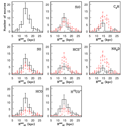
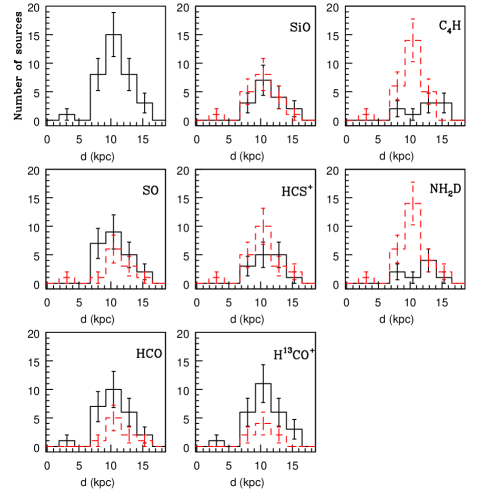
Figure 2: Histograms comparing the Galactocentric (left panels) and heliocentric (right panels) distance for detected (solid line) and undetected (red-dashed line) sources in the molecular species labelled in the top right corner of each panel. The top left panel includes the whole sample without distinguishing between detections and non-detections. Poissonian errorbars are given in each bin.

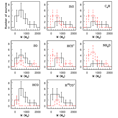
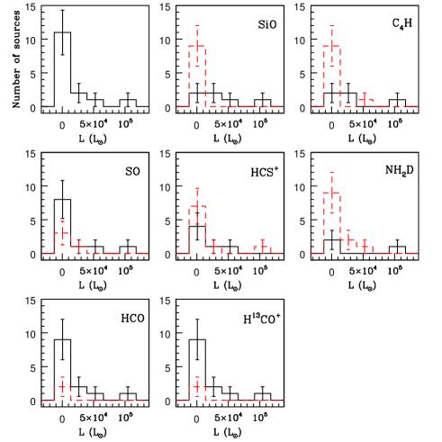
Figure 3: Same as Fig. 2 for H₂ mass ($M$, left panels), and the bolometric luminosity ($L$ right panels). Both parameters are derived from Herschel observations and are given in Table 1.

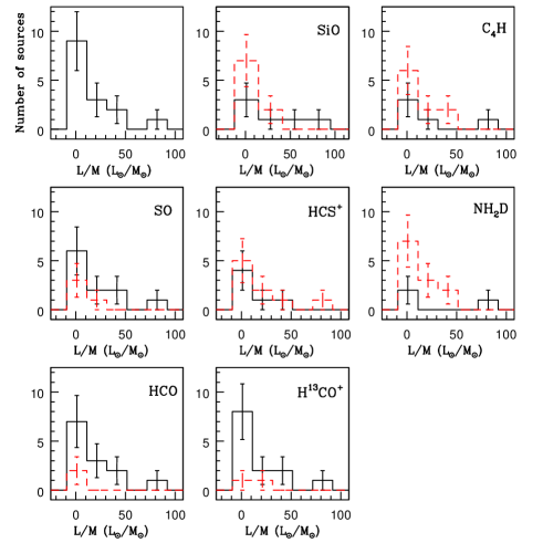
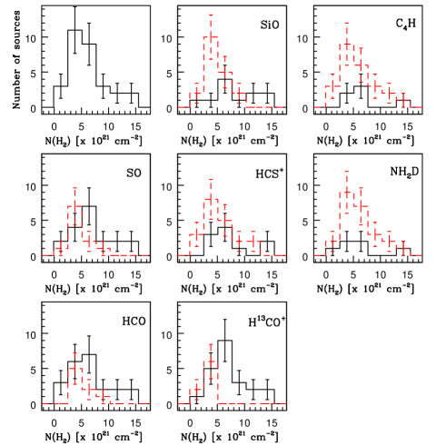
Figure 4: Same as Fig. 3 for the luminosity-to-mass ratio ($L/M$, left panels) and the H₂ column density ($N({\rm H_{2}})$, right panels). The latter, derived by Blair et al. (2008), is given in Table 1.

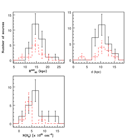
Figure 5: Histograms showing the distribution of the sources associated (solid line) or not associated (red-dashed line) with HCO⁺ $J=1-0$ high-velocity wings as a function of $R^{new}_{\rm GC}$, $d$, and $N({\rm H_{2}})$). Sources tentatively associated with wings are included in the solid-line histograms.

5.1 Statistical analysis

Here we analyse statistically the detection of the various molecular species as a function of the physical properties of the targets, i.e.: updated Galactocentric and heliocentric distance (Table 6), H₂ column density (Table 1) and, for the sources belonging to the Hi-GAL catalogue, mass, luminosity, and luminosity-to-mass ratio (Table 1). A thorough analysis of each molecular species and of the parameters that can be derived from them (in particular column densities and abundances) goes beyond the scope of this presentation paper and will be performed in forthcoming papers.

Figure 2 shows the histograms with the detected and undetected sources in each molecular tracer as a function of $R_{\rm GC}$ (left panels) and $d$ (right panels). We include only molecular species for which the detection rate is in between $20-80\%$, so that the statistical comparison between the two groups (detected and undetected sources) is possible. The distribution for detected and undetected sources is similar, and similar also to the total one for all molecules. Marginal differences between the two distributions are tentatively seen in C₄H and NH₂D, but the detected sources are less than $\sim 30\%$ in both molecules and hence the comparison must be very cautious here.

Figures 3 and 4 investigate, for each species, statistically significant differences for detected and undetected sources as a function of $M$, $L$, luminosity-to-mass ratio ($L/M$), and $N$(H₂). In particular, $L/M$ is often used as an evolutionary tracer because expected to increase with time, as the envelope mass decreases while the bolometric luminosity increases during collapse. Overall, we do not find clear differences between the distribution of detected and undetected sources also in this case, even though the sources with high $L$ and $N(\rm H_{2})$ tend to be always detected. We suggest a tentative, but interesting, difference in the plots showing the results for SiO: the sources associated with SiO emission tend to have higher $M$, $L$, and $N(\rm H_{2})$. This could be interpreted as the result of a more active star formation activity in the most luminous and massive objects, as already suggested by López-Sepulcre et al. (2011) in 57 high-mass molecular clumps mostly located in the inner Galaxy.

In this respect, we also investigated if the presence of high-velocity blue- and red-shifted emission in the HCO⁺ $J=1-0$ line depends somehow on $R^{new}_{\rm GC}$, $d$, and/or $N(H_{2})$. Figure 5 shows the comparative histograms which, overall, again do not show a clear difference between the distribution of detected and undetected sources as a function of the mentioned parameters, indicating once more that protostellar activity does not seem to depend on $R_{\rm GC}$. Very similar distributions are also found for detected and undetected sources as a function of $N({\rm H_{2}})$, even though the detected sources tend to be associated with sources with higher $N({\rm H_{2}})$, which can be due to sensitivity reasons: the high-velocity wings are detected more easily towards more massive outflows. As for possible differences between sources with or without wings as a function of $M$, $L$, and $L/M$, unfortunately, only two sources with available $M$ and $L$ are undetected in HCO⁺ high-velocity wings (WB89-083 and WB89-529), hence a statistical comparison cannot be performed.

5.2 Towards a redefinition of the Galactic Habitable Zone?

Our study clearly supports previous claims that organic molecules and tracers of protostellar activity are ubiquitous in the Galaxy (Blair et al. 2008, Bernal et al. 2021). As said in Sect. 1, the outermost edge of the Milky Way was believed to be a hostile environment for both planets and (biogenic) organic molecules because the metallicity, i.e. the abundance of elements heavier than helium, is too low. Hence, the OG was excluded from the GHZ. This latter was defined as the region with the most favourable conditions for the development and long-term maintenance of complex life comparable to terrestrial animals and complex plants (Gonzalez et al. 2001).

Based on this definition, two properties were invoked: (1) a sufficient amount of heavy elements to form rocky planets and the basic bricks of biogenic molecules, and (2) a low concentration of high energy, potentially disruptive events such as supernovae and gamma-ray bursts, which may cause life perturbation and extinction. Property (1) sets the outer boundaries of the GHZ, which depends on the metallicity gradient in the radial disk. Property (2) sets the inner boundaries, as the concentration of potentially disruptive events would decrease with the distance from the centre of the Milky Way. Combining these two requirements, the GHZ of the Milky Way was proposed to be an annulus of a few kpc centred at 8 kpc from the Galactic Centre (Spitoni et al. 2017), even though a hot debate is on-going on this subject. E.g. Spinelli et al. (2021) have proposed that the boundaries of the GHZ change with Galaxy evolution, and that in the last four billion years the safer region to avoid disruptive events is $R_{\rm GC}\sim 2-8$ kpc, while the OG was safer for the development of living organisms before that time.

Therefore, the boundaries of the GHZ are not rigid limits but rather based on probability arguments, and the ubiquitous presence of rocky planets in the Galaxy, independent on the metallicity of the host environment (see Sect. 1 and references therein), shows the need for a re-discussion, at least, of property (1). The idea of a redefinition of the GHZ is already discussed in Blair et al. (2008) and Bernal et al. (2021), based on observations of single organic molecules (H₂CO in Blair et al. 2008, CH₃OH in Bernal et al. 2021) in the OG. The CHEMOUT project, thanks to observations of multiple species and lines, obtained with the same setup(s) for all sources, place us in a position to expand this discussion by comparing in a consistent way the observational properties of many molecules (possibly) chemically connected. In future papers, by comparing key observational parameters (in particular column densities and fractional abundances) with chemical models with adapted metallicity, we will better understand what are the main formation routes, and whether they are similar or different to those known to be efficient in the local and inner Galaxy. In this respect, the partial results presented in this work, and the similar recent observational findings of Bernal et al. (2021), suggest that the capacity of the environment to form organic (both simple and complex) molecules is independent on metallicity. Thus, the outer boundaries of the GHZ are likely much wider than previously claimed because the basic bricks of organic chemistry can be easily found even at the outer edge of the Milky Way.

6 Conclusions

Table 6: New Galactocentric ($R^{new}_{\rm GC}$) and heliocentric ($d$) distances computed from the peak velocity ($V_{\rm p}$) of the c-C₃H₂ $J_{K_{a},K_{b}}=2_{1,2}-1_{0,1}$ line as explained in Sect. 4.3.

source	Longitude	$V_{\rm p}^{(a)}$	$R^{new}_{\rm GC}$	$d$
	$\deg$	km s-1	kpc	kpc
WB89-315	118.0	–95.1(0.3)(b)	16.3	10.7
WB89-379	124.6	–89.16(0.06)	16.4	10.2
WB89-380	124.6	–86.68(0.04)	16.0	9.7
WB89-391	125.8	–86.10(0.02)	16.1	9.7
WB89-399	128.8	–82.15(0.05)	16.0	9.4
WB89-437	135.3	–72.14(0.06)	15.7	8.6
WB89-440	135.6	–71.88(0.05)	15.7	8.6
WB89-501	145.2	–58.43(0.04)	15.6	8.0
WB89-529	149.6	–59.8(0.2)	17.8	10.1
WB89-572	156.9	–47.4(0.1)	18.3	10.3
WB89-621	168.1	–25.68(0.07)	18.9	10.6
WB89-640	167.1	–24.93(0.08)	16.8	8.6
WB89-670	173.0	–17.65(0.01)	23.4	15.1
WB89-705	174.7	–12.20(0.01)	20.5	12.2
WB89-789	195.8	34.25(0.05)	19.1	11.0
WB89-793	195.8	30.5(0.2)	16.9	8.7
WB89-898	217.6	63.5(0.1)	15.8	8.4
19423+2541	61.72	–72.58(0.04)	13.5	15.3
19383+2711	62.58	–70.2(0.2)	13.2	14.8
19383+2711-b(c)	62.58	–65.6(0.2)	12.7	14.2
19489+3030	66.61	–69.29(0.05)	12.9	13.7
19571+3113	68.15	–61.7(0.1)	12.2	12.5
19571+3113-b(c)	68.15	–66.2(0.1)	12.5	13.0
20243+3853	77.6	–73.21(0.05)	12.8	11.7
WB89-002	85.41	–2.83(0.09)	8.65	3.1
WB89-006	86.27	–90.38(0.05)	14.3	12.2
WB89-014	88.99	–96.0(0.1)	14.9	12.5
WB89-031	88.06	–88.89(0.08)	14.1	11.7
WB89-035	89.94	–77.56(0.03)	13.1	10.1
WB89-040	90.68	–62.38(0.05)	11.9	8.3
WB89-060	95.05	–83.7(0.15)	13.6	10.1
WB89-076	95.25	–97.07(0.02)	15.1	11.8
WB89-080	95.44	–74.1(0.2)	12.8	8.9
WB89-083	96.08	–93.76(0.04)	14.7	11.2
WB89-152	104.0	–88.5(0.2)	14.4	9.8
WB89-283	114.3	–94.69(0.06)	15.8	10.4
WB89-288	114.3	–101.0(0.1)	16.8	11.5

^(a) obtained from the Gaussian fits in Table A-2. Uncertainties derived from the fitting procedure are quoted in parentheses;
^(b) source undetected in c-C₃H₂ and in any other optically thin transition (Table 3). We use the $V_{\rm LSR}$ given in Blair et al. (2008);
^(c) second velocity feature (see Fig. B-2).

With the IRAM-30m Telescope, we have searched for emission of simple organic molecules and tracers of star-formation activity in 35 star-forming regions of the OG. Their (updated) Galactocentric distances are in between $\sim 8.7$ and $\sim 23.4$ kpc. We report the detection of several simple organic molecules (HCN, HCO⁺, H¹³CO⁺, HCO, HCS⁺, C₄H) and of the complex hydrocarbon CH₃CCH. We also detected transitions of SO, CCS, NH₂D, and SiO. In the HCO⁺ $J=1-0$ line profiles, we detected high velocity blue- and red-shifted emission in 25 sources ($71\%$), indicating the presence of protostellar outflows in a large fraction of the targets. Moreover, most of the sources showing emission in SiO and SO are associated with high velocity wings in HCO⁺, indicating that also in the low metallicity environment of the OG these molecular species are good tracers of outflows and protostellar activity. We have investigated whether the detection in the various molecules depends on some physical properties of the sources, such as $R_{\rm GC}$, $d$, $M$, $L$, $L/M$, and $N(\rm H_{2})$. Overall, no clear trends have been found, indicating that the presence of the molecules analysed in this work do not depend neither on the Galactocentric distance nor on other physical parameters, even though in some cases the statistics is low and does not allow us to derive firm conclusions. Similarly, no significant differences have been found between sources with or without high velocity blue- and red-shifted wings in the HCO⁺ line profiles. We suggest a tentative difference for SiO, for which the detected sources are more likely associated with more massive and luminous objects. Our study clearly supports previous claims that organic molecules and tracers of protostellar activity are ubiquitous in the Galaxy. Our results and the additional, growing evidence that the formation of terrestrial planets is possible also at low metallicity, put into question former, stringent definitions of GHZ, in which the capacity of the environment to form both organic and other pre-biotic molecules is not taken into account.

Appendix A: spectrum and line intensities of WB89-437

In this appendix, we show the full spectrum observed at 3 mm towards WB89-437 (Fig. A-1), and zoomed spectral windows around the faintest detected lines (Fig. A-2). The intensities of the detected transitions are listed in Table A-1.

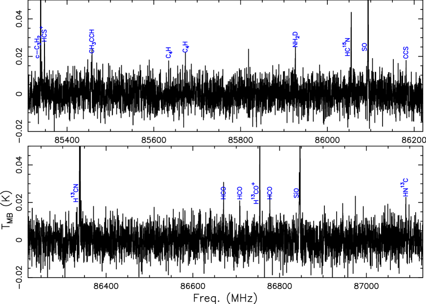
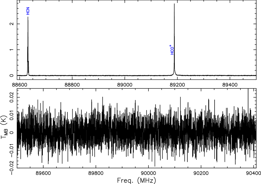
Figure A-1: Full 3 mm spectrum obtained towards WB89-437. Detected lines of the molecules listed in Table 3 are indicated. The spectral parameters of all transitions are given in Table 4.

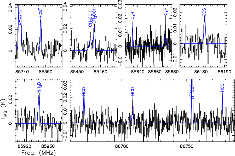
Figure A-2: Selected spectral windows around faint lines in the spectrum at 3 mm of WB89-437. The blue curve in each panel shows the best Gaussian fit to the detected lines.

Table A-1: Peak intensities, in K ($T_{\rm MB}$ units) of the transitions detected towards WB89-437 (Figs. A-1 and  A-2), obtained from Gaussian fits performed with class. The calibration errors are indicated in parentheses.

c-C3H2	HCS+	CH3CCH(a)	C4H(b)	CCS	HCO(c)
0.1(0.01)	0.030(0.003)	0.022(0.02)	0.017(0.002)	0.017(0.002)	0.024(0.003)
H13CO+	HCN(d)	HCO+	NH2D	SO	SiO
0.10(0.01)	2.3(0.3)	2.7(0.3)	0.025(0.003)	0.17(0.02)	0.060(0.007)

^(a) $K=0$ line (Table 4);
^(b) strongest group of unresolved hyperfine components $J=19/2-17/2$ (Table 4);
^(c) strongest resolved hyperfine component $J=3/2-1/2$, $F=2-1$ (Table 4);
^(d) strongest resolved hyperfine component $F=2-1$ (Table 4).

Appendix B: Gaussian analysis of the HCO⁺ and c-C₃H₂ lines

We show in this appendix the spectra of HCO⁺ $J=1-0$ and c-C₃H₂ $J_{K_{a},K_{b}}=2_{1,2}-1_{0,1}$ (Figs. B-1 and B-2), analysed in Sects. 4.2 and 4.3, respectively, and the line parameters obtained from Gaussian fits to the lines (Tables A-1 and A-2).

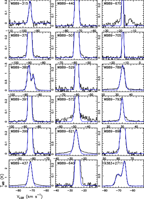
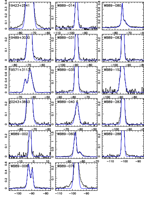
Figure B-1: Spectra of HCO⁺ $J=1-0$ obtained with the IRAM-30m telescope towards the sources listed in Table 1. The blue curve in each frame represents the best Gaussian fit to the line. For spectra with two intensity peaks, a double Gaussian fit has been performed. In some cases, the y-axis has been reduced to highlight the (tentative) red- and blue-shifted high-velocity non-Gaussian wings.

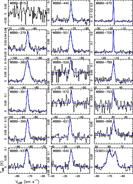
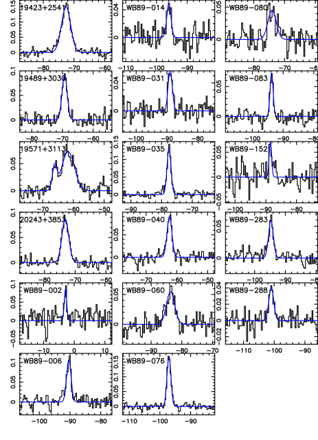
Figure B-2: Same as Fig. B-1 for c-C₃H₂ $J_{K_{a},K_{b}}=2_{1,2}-1_{0,1}$.

Table B-1: Best fit parameters from Gaussian fits to the HCO⁺ $J=1-0$ lines shown in Fig. B-1. Uncertainties derived from the fitting procedure are quoted in parentheses.

source	$\int T_{\rm MB}{\rm d}V$(1)	$V_{\rm p}$(2)	FWHM(3)	$T_{\rm MB}^{\rm p}$(4)
	K km s-1	km s-1	km s-1	K
WB89–315	0.46(0.02)	–94.91(0.04)	2.07(0.09)	0.209
WB89–379	2.19(0.01)	–89.41(0.01)	2.20(0.01)	0.936
WB89–380	4.057(0.001)	–87.36(0.01)	2.60(0.01)	1.47
WB89–380-b(a)	1.868(0.001)	–84.14(0.02)	2.0(0.2)	0.898
WB89–391	2.232(0.007)	–86.12(0.01)	1.94(0.01)	1.08
WB89–399	2.97(0.02)	–81.94(0.01)	2.03(0.01)	1.38
WB89–437	8.8(0.12)	–71.34(0.02)	3.06(0.05)	2.70
WB89–440	2.72(0.01)	–71.90(0.01)	2.07(0.01)	1.24
WB89–501	2.99(0.01)	–58.22(0.01)	2.28(0.01)	1.23
WB89–529	1.85(0.02)	–59.69(0.01)	1.82(0.02)	0.956
WB89–572	1.30(0.03)	–47.74(0.04)	2.9(0.1)	0.415
WB89–621	4.57(0.08)	–25.62(0.03)	3.76(0.08)	1.14
WB89–640	3.35(0.02)	–24.78(0.01)	2.27(0.02)	1.39
WB89–670	1.15(0.02)	–17.69(0.01)	0.97(0.02)	1.12
WB89–705	0.57(0.01)	–12.17(0.02)	1.40(0.03)	0.381
WB89–789	3.77(0.04)	34.14(0.02)	3.37(0.04)	1.05
WB89–793	2.90(0.05)	29.91(0.02)	2.25(0.05)	1.21
WB89–898	1.95(0.02)	63.31(0.02)	3.17(0.03)	0.576
19423+2541	8.48(0.03)	–72.79(0.02)	3.81(0.02)	2.09
19383+2711	2.75(0.03)	–70.22(0.02)	4.29(0.03)	0.601
19383+2711-b(a)	3.60(0.02)	–65.81(0.01)	2.82(0.01)	1.20
19489+3030	2.74(0.01)	–69.09(0.01)	2.70(0.01)	0.953
19571+3113	0.82(0.01)	–65.90(0.01)	1.93(0.03)	0.400
19571+3113-b(a)	2.70(0.02	–62.21(0.01)	3.42(0.03)	0.741
20243+3853	2.89(0.01)	–73.20(0.01)	3.33(0.02)	0.816
WB89–002	0.75(0.02)	–2.50(0.02)	1.48(0.05)	0.480
WB89–006	1.30(0.02)	–92.23(0.02)	2.10(0.04)	0.579
WB89–006-b(a)	0.78(0.02)	–89.61(0.02)	1.55(0.05)	0.470
WB89–014	0.88(0.02)	–95.93(0.02)	1.79(0.04)	0.464
WB89–031	1.12(0.01)	–89.29(0.01)	1.53(0.02)	0.690
WB89–035	1.84(0.01)	–77.62(0.01)	1.86(0.01)	0.930
WB89–040	0.64(0.02)	–62.22(0.03)	2.88(0.09)	0.210
WB89–060	3.47(0.04)	–85.13(0.01)	2.07(0.03)	1.57
WB89–060-b(a)	0.88(0.04)	–81.61(0.06)	2.7(0.2)	0.307
WB89–076	2.00(0.03)	–97.43(0.02)	2.74(0.04)	0.685
WB89–080	0.71(0.03)	–74.77(0.01)	1.10(0.03)	0.603
WB89–080-b(a)	1.18(0.04)	–73.61(0.08)	5.1(0.2)	0.218
WB89–083	1.210(0.008)	–93.91(0.04)	1.59(0.01)	0.715
WB89–152	1.21(0.03)	–88.56(0.04)	3.1(0.1)	0.368
WB89–283	1.51(0.01)	–94.45(0.01)	1.78(0.01)	0.796
WB89–288	1.15(0.01)	–100.9(0.01)	1.74(0.02)	0.620

⁽¹⁾ line integrated intensity;
⁽²⁾ peak velocity;
⁽³⁾ full width at half maximum;
⁽⁴⁾ intensity peak;
^(a) second velocity feature.

Table B-2: Best fit parameters from Gaussian fits to the c-C₃H₂ $J_{K_{a},K_{b}}=2_{1,2}-1_{0,1}$ lines shown in Fig. B-2. Uncertainties derived from the fitting procedure are quoted in parentheses.

source	$\int T_{\rm MB}{\rm d}V$(1)	$V_{\rm p}$(2)	FWHM(3)	$T_{\rm MB}^{\rm p}$(4)
	K km s-1	km s-1	km s-1	K
WB89–315	$\leq 0.04$	–	–	$\leq 0.03$
WB89–379	0.121(0.007)	–89.16(0.06)	2.0(0.2)	0.057
WB89–380	0.63(0.02)	–86.68(0.04)	4.0(0.1)	0.148
WB89–391	0.220(0.006)	–86.10(0.02)	1.58(0.05)	0.131
WB89–399	0.36(0.02)	–82.15(0.05)	2.2(0.1)	0.151
WB89–437	0.32(0.01)	–72.14(0.06)	3.0(0.2)	0.099
WB89–440	0.16(0.01)	–71.88(0.05)	1.6(0.1)	0.092
WB89–501	0.24(0.01)	–58.43(0.04)	2.2(0.1)	0.102
WB89–529	0.11(0.02)	–59.8(0.2)	2.0(0.4)	0.051
WB89–572	0.06(0.01)	–47.4(0.1)	1.0(0.3)	0.050
WB89–621	0.13(0.01)	–25.68(0.07)	2.0(0.2)	0.060
WB89–640	0.32(0.02)	–24.93(0.08)	2.5(0.2)	0.121
WB89–670	0.28(0.01)	–17.65(0.01)	0.68(0.02)	0.387
WB89–705	0.196(0.008)	–12.20(0.01)	0.67(0.03)	0.275
WB89–789	0.23(0.01)	34.25(0.05)	1.9(0.1)	0.114
WB89–793	0.19(0.03)	30.5(0.2)	2.1(0.6)	0.085
WB89–898	0.17(0.02)	63.5(0.1)	2.6(0.4)	0.061
19423+2541	0.56(0.01)	–72.58(0.04)	3.5(0.1)	0.150
19383+2711	0.35(0.03)	–70.2(0.2)	4.2(0.4)	0.079
19383+2711-b(a)	0.23(0.03)	–65.6(0.2)	3.1(0.3)	0.069
19489+3030	0.19(0.01)	–69.29(0.05)	2.0(0.1)	0.092
19571+3113	0.37(0.02)	–61.7(0.1)	4.8(0.3)	0.072
19571+3113-b(a)	0.08(0.01)	–66.2(0.1)	1.8(0.3)	0.043
20243+3853	0.24(0.01)	–73.21(0.05)	2.6(0.1)	0.087
WB89–002	0.08(0.02)	–2.8(0.1)	0.9(0.2)	0.087
WB89–006	0.20(0.01)	–90.38(0.05)	1.7(0.2)	0.107
WB89–014	0.08(0.01)	–96.0(0.1)	1.6(0.3)	0.048
WB89–031	1.00(0.01)	–88.89(0.08)	1.6(0.2)	0.059
WB89–035	0.21(0.08)	–77.56(0.03)	1.50(0.07)	0.135
WB89–040	0.18(0.01)	–62.38(0.05)	1.9(0.1)	0.090
WB89–060	0.18(0.02)	–83.7(0.2)	3.1(0.3)	0.055
WB89–076	0.270(0.008)	–97.07(0.02)	1.49(0.05)	0.170
WB89–080	0.15(0.02)	–74.1(0.2)	3.2(0.5)	0.045
WB89–083	0.090(0.007)	–93.76(0.04)	1.2(0.1)	0.073
WB89–152	0.07(0.02)	–88.5(0.2)	1.0(0.5)	0.070
WB89–283	0.12(0.01)	–94.69(0.06)	1.9(0.2)	0.059
WB89–288	0.08(0.01)	–101.0(0.1)	1.8(0.3)	0.041

⁽¹⁾ line integrated intensity;
⁽²⁾ peak velocity;
⁽³⁾ full width at half maximum;
⁽⁴⁾ intensity peak;
^(a) second velocity feature.

Appendix C: kinematic distances derived from the rotation curve of Reid et al. (2019).

Table C-1: Kinematic Galactocentric and heliocentric distances derived from the rotation curve of Reid et al. (2019).

source	$R^{new}_{\rm GC}$(1)	$d$(1)
	kpc	kpc
WB89-315	14.63	8.72
WB89-379	14.66	8.21
WB89-380	14.35	7.86
WB89-391	14.43	7.86
WB89-399	14.34	7.55
WB89-437	14.02	6.79
WB89-440	14.04	6.80
WB89-501	13.92	6.22
WB89-529	15.58	7.79
WB89-572	15.74	7.71
WB89-621	15.44	7.17
WB89-640	14.1	5.84
WB89-670	17.04	8.72
WB89-705	14.63	6.30
WB89-789	18.66	10.49
WB89-793	16.57	8.38
WB89-898	14.93	7.42
19423+2541	12.13	13.60
19383+2711	12.28	13.63
19489+3030	11.84	12.34
19571+3113	11.26	11.27
20243+3853	11.84	10.37
WB89-002	8.369	1.54
WB89-006	13.02	10.55
WB89-014	13.49	10.74
WB89-031	12.91	10.13
WB89-035	12.03	8.67
WB89-040	11.04	7.12
WB89-060	12.5	8.59
WB89-076	13.64	10.05
WB89-080	11.81	7.60
WB89-083	13.35	9.57
WB89-152	13.07	8.24
WB89-283	14.24	8.60
WB89-288	14.98	9.47

⁽¹⁾ We adopted the same Longitude and $V_{\rm p}$ (for sources having two velocity features, only the main one is used) as in Table 6.