Computing Bounds on $L_{\infty}$-induced Norm for Linear Time Invariant Systems Using Homogeneous Lyapunov Functions

Abstract

Quadratic Lyapunov function has been widely used in the analysis of linear time invariant (LTI) systems ever since it has shown that the existence of such quadratic Lyapunov function certifies the stability of the LTI system. In this work, the problem of finding upper and lower bounds for the $L_{\infty}$-induced norm of the LTI system is considered. Quadratic Lyapunov functions are used to find the star norm, the best upper on the $L_{\infty}$-induced norm, by bounding the unit peak input reachable sets by inescapable ellipsoids. Instead, a more general class of homogeneous Lyapunov functions is used to get less conservative upper bounds on the $L_{\infty}$-induced norm and better conservative approximations for the reachable sets than those obtained using standard quadratic Lyapunov functions. The homogeneous Lyapunov function for the LTI system is considered to be a quadratic Lyapunov function for a higher-order system obtained by Lifting the LTI system via Kronecker product. Different examples are provided to show the significant improvements on the bounds obtained by using Homogeneous Lyapunov functions.

I INTRODUCTION

For single-input,single-output (SISO) continuous-time invariant systems, the ${L}_{\infty}$-induced norm, the signal peak-to-peak gain of a transfer function, is the $\ell_{1}$ norm that can be computed by $\int_{0}^{\infty}|h(t)|\text{dt}$, where $h(t)$ is the impulse response of the system. Shamma [1] shows that there does not exist a closed form expression for the $\ell_{1}$ norm of the LTI system. Given the state space model of the system, an approximate value of the $\ell_{1}$ norm can be obtained by only simulation. The problem is to find the final time that provides an accurate approximation for the integration value. This fact motivates the search for alternative methods to get reliable upper bounds for the $\ell_{1}$ norm. Authors in [2] introduce the star-norm to provide a valid upper bound for the $\ell_{1}$ norm by the construction of inescapable ellipsoids using quadratic lyapunov functions. But the star-norm calculated in [2] represents a very conservative upper bound on the $\ell_{1}$ norm for stiff systems, such as introduced in [3]. This motivated us to introduce new methods for computing more conservative approximations for the $\ell_{1}$ norm of linear time invariant systems.

Several methods in the control theory literature are used in computing $\ell_{1}$ norm including the originating article [4] in which the author computes the $\ell_{1}$ norm for both discrete and continuous time systems with some initial results on controller design for disturbance rejection. In [5], a comparison between the $L_{\infty}$ induced norm of a discrete system and its RMS gain (the maximum magnitude of the its frequency response) is made to see how this difference affects $\mathbf{H}_{\infty}$ optimal controller design. An improved upper and lower bounds for a discrete time system ’s $\ell_{1}$ norm are introduced in [6] . Based on these bounds, the worst case $L_{\infty}$ induced norm of the discrete-time systems with diagonal perturbations can be computed accurately. The $\ell_{1}$ optimal controller design for discrete-time MIMO systems is introduced in [7]. The controller is designed to make the system internally stable and optimally track a bounded input signal. The results in [7] are extended to $\ell_{1}$ optimal controller design for continuous time systems in [8]. The problem of $\ell_{1}$ optimal controller with full state feedback is considered in [9] where author showed that instead of using state feedback dynamic linear controller with arbitrary higher order, the $\ell_{1}$ optimal controller can be nonlinear memoryless static feedback.

In this note, we introduce different techniques in approximating the $\ell_{1}$ norm of LTI systems. The method used in [2] depends on computing the star-norm by using quadratic Lyapunov function to bound the reachable sets. This methods produces good bounds for some systems. But for stiff systems, as we will show later, these bounds become more conservative. Our approach is based on using higher order homogeneous Lyapunov function in generating the inescapable ellipsoids to reduce the conservatism in the computed upper bound of the $\ell_{1}$ norm. This higher order Lyapunov function can be considered as a quadratic Lyapunov function for a higher order ”lifted” system. The authors of [10] show how the lifted systems are generated for linear time varying systems using a recursive algorithm based on the Kronecker product. In addition, they show that the higher order homogeneous Lyapunov function that certifies stability for linear varying can be considered as a quadratic Lyapunov function for the lifted system to a higher degree. The homogeneous Lyapunov functions are also used to obtain better approximations for some performance metrics for linear time varying systems in [11]. The authors show that the bounds on system’s peak norms obtained using higher order homogeneous Lyapunov function are more accurate and less conservative than the bounds resulted using quadratic Lyapunov functions. In [11], the effect of control inputs is considered in the lifting process. In this work, we extend the work introduced in [10] and [11] and use homogeneous Lyapunov function to compute less conservative upper bounds for the linear time invariant system’s $\ell_{1}$ norm. These bounds are less than the bounds introduced in [2]. In this work, the reachable sets for LTI systems using unit peak input are approximated using higher order homogeneous Lyapunov functions, then the star norm is computed based on the generated ellipsoid to get better approximation for the system’s $\ell_{1}$ norm. Additionally, we introduce another technique to better approximate the integral value $\int_{0}^{\infty}|Ce^{At}B|\text{dt}$ by calculating the integral to a specific time $T_{0}$ then approximate an upper bound for the remaining integral $\int_{T_{0}}^{\infty}|Ce^{At}B|\text{dt}$ by computing the star-norm for a an equivalent new system. The upper bound for the remaining integral is also improved by lifting the new system. We show that it is more powerful that computing the star norm of the original system directly. To illustrate the results, we compute upper bounds on $\ell_{1}$ norm for different types of systems like: systems with high damping, systems with low damping and systems with stiff mass matrix, by using our proposed approaches that gives very accurate approximations compared with the methods introduced in the literature.

II Notation

Denote the sets of non-negative and positive integers by $\mathbb{Z}_{+}$ and $\mathbb{Z}_{++}$ respectively. $\mathbb{R}_{+}$ and $\mathbb{R}_{++}$ denotes the set of non-negative and positive real numbers respectively. The set of positive definite $n\times n$ matrices is denoted by $\mathbb{S}_{++}^{n}\subset\mathbb{R}^{n\times n}$. For $P\in\mathbb{R}^{n\times n}$, $P\succ 0$ means that $P$ is a positive definite matrix and the function $V(x)=x^{T}Px$ is positive for all non-zero $x\in R^{n}$. The $n\times n$ identity matrix is denoted by $I_{n}$.

II-A Kroncker product

For matrices $A\in\mathbb{R}^{n\times m}$ and $B\in\mathbb{R}^{p\times q}$, the Kroncker product of $A$ and $B$ is denoted by $A\otimes B\in\mathbb{R}^{np\times mq}$ and is given by

$$A\otimes B:=\left[\begin{array}[]{ccc}a_{11}B&\cdots&a_{1m}B\\ \vdots&\ddots&\vdots\\ a_{n1}B&\cdots&a_{nm}B\end{array}\right]$$ (1)

where $A$ matrix entries are represented via subscript. We will introduce some properties of the kroncker product defined in [12] and [13]. For $A\in\mathbb{R}^{n\times m}$, the $d\textsuperscript{th}$ kroncker power $A^{\otimes d}$ for all $d\in\mathbb{Z}_{++}$ is defined recursively with a base $A^{\otimes 0}=1$ by:

$$A^{\otimes 1} =A$$ (2)

$$A^{\otimes d} =A\otimes A^{\otimes(d-1)},\quad d=2,3,\dots$$

The following important properties of kroncker product are used in this work:

$$A\otimes(B+C)=A\otimes B+A\otimes C$$ (3a)

$$(A\otimes B)(C\otimes D)=(AC)\otimes(BD)$$ (3b)

$$(AB)^{\otimes n}=A^{\otimes n}B^{\otimes n}$$ (3c)

where all matrices $A$,$B$,$C$ and $D$ are with proper dimensions that permit the formation of products $AC$ and $BD$. In [12],corollary (7) states that property (3b) can be generalized as

$$A_{1}B_{1}\otimes A_{2}B_{2}\otimes\cdots\otimes A_{n}B_{n}\\ =\left(A_{1}\otimes A_{2}\otimes\cdots\otimes A_{n}\right)\left(B_{1}\otimes B_{2}\otimes\cdots\otimes B_{n}\right),$$ (4)

such that all matrices $(A_{1},A_{2},\dots A_{n})$ and $(B_{1},B_{2},\dots B_{n})$ are with proper dimensions that allows all multiplications in the right hand side.

The $d\textsuperscript{th}$ kroncker sum of a symmetric matrix $A\in\mathbb{R}^{n\times n}$ is defined by

$$A^{\oplus d}=\sum_{k=1}^{d}I_{n}^{\otimes(k-1)}\otimes A\otimes I_{n}^{(d-k)}.$$ (5)

For example,

$$A^{\oplus 3} =I_{n}^{\otimes 0}\otimes A\otimes I_{n}^{\otimes 2}+I_{n}^{\otimes 1}\otimes A\otimes I_{n}^{\otimes 1}+I_{n}^{\otimes 2}\otimes A\otimes I_{n}^{\otimes 0}$$ (6)

$$=A\otimes I_{n}\otimes I_{n}+I_{n}\otimes A\otimes I_{n}+I_{n}\otimes I_{n}\otimes A.$$

II-B Norms

For a vector $v\in\mathbb{R}^{n}$, we define the ${L}_{\infty}$ norm as

$$\|v\|_{\infty}=\sup_{i}\left|v_{i}\right|$$ (7)

where $v=[v_{1},v_{2},\dots,v_{n}]^{T}$. The function space $\mathcal{L}_{\infty}$ is defined as the set of functions $f(t)$ for which the $L_{\infty}$ norm:

$$\|f\|_{\infty}=\sup_{t\in\mathbb{R}+}\|f(t)\|_{\infty}$$ (8)

is bounded. The $L_{\infty}$-induced norm of an operator $\mathcal{G}$ which maps $u$ to $y=\mathcal{G}u$ is defined by

$$\|\mathcal{G}\|_{\infty}=\sup_{\underset{u\neq 0}{u\in\mathcal{L}_{\infty}}}\frac{\|\mathcal{G}u\|_{\infty}}{\left\|u\right\|_{\infty}}$$ (9)

Given that the operator $\mathcal{G}$ is considered as the following single-input single-output linear time invariant system

$$\mathcal{G}:\left\{\begin{array}[]{l}\dot{x}=Ax+Bu\\ y=Cx\end{array}\right.$$ (10)

where $x\in\mathbb{R}^{n}$ and ($A\in\mathbb{R}^{n\times n},B\in\mathbb{R}^{n\times 1}$ and $C\in\mathbb{R}^{1\times n}$ ) are the system’s matrices, the $L_{\infty}$-induced norm in (9) is the $\ell_{1}$ norm of the system in (10) which can be computed as

$$\|\mathcal{G}\|_{1}=\int_{0}^{\infty}|h(t)|\text{dt},$$ (11)

where $h(t)$ is the impulse response of the system and can be computed as:

$$h(t)=Ce^{At}B$$ (12)

III Dynamical system lifting

In this section, we incorporate the results introduced in [10] and [11] on lifting the system dynamics from the original space to a higher order space. Additionally, we consider the control input in the lifting procedure.

III-A Lifting procedure

First, given the LTI system in (10), the state vector $x$ is lifted to $x^{\otimes d}$ where $d$ is the lifting order. Then, the chain rule is applied to obtain the derivative of the lifted state vector $x^{\otimes d}$ with respect to time as

$$\frac{d}{dt}x^{\otimes d} =\sum_{k=1}^{d}x^{\otimes{(k-1)}}\otimes\dot{x}\otimes x^{\otimes(d-k)}$$ (13)

$$=\sum_{(k=1)}^{d}x^{\otimes{k-1}}\otimes(Ax+Bu)\otimes x^{\otimes(d-k)}.$$

By using property (3a), equation (13) can be written as

$$\frac{d}{dt}x^{\otimes d} =\sum_{k=1}^{d}x^{\otimes{(k-1)}}\otimes Ax\otimes x^{\otimes(d-k)}$$ (14)

$$+\sum_{k=1}^{d}x^{\otimes{(k-1)}}\otimes Bu\otimes x^{\otimes(d-k)}.$$

Since $x=I_{n}x$, property (3c) can be used. Therefore, (14) becomes

$$\frac{d}{dt}x^{\otimes d} =\sum_{k=1}^{d}(I_{n}^{\otimes{(k-1)}}x^{\otimes{(k-1)}})\otimes Ax\otimes(I_{n}^{\otimes(d-k)}x^{\otimes(d-k)})$$ (15)

$$+\sum_{k=1}^{d}(I_{n}^{\otimes{(k-1)}}x^{\otimes{(k-1)}})\otimes Bu\otimes(I_{n}^{\otimes(d-k)}x^{\otimes(d-k)}),$$

hence property (4) can be applied in (15) to be

$$\frac{d}{dt}x^{\otimes d} =\sum_{k=1}^{d}(I_{n}^{\otimes(k-1)}\otimes A\otimes I_{n}^{\otimes(d-k)})x^{\otimes d}$$ (16)

$$+\sum_{k=1}^{d}(I_{n}^{\otimes(k-1)}\otimes B\otimes I_{n}^{\otimes(d-k)})ux^{\otimes(d-1)}.$$

By using (6), (16) can be summarized as

$$\frac{d}{dt}x^{\otimes d}=A^{\oplus d}x^{\otimes d}+B^{\oplus d}ux^{\otimes(d-1)}.$$ (17)

The output equation in (10) is lifted as

$$y^{\otimes d}=C^{\otimes d}x^{\otimes d}.$$ (18)

To summarize this section, the LTI system (10) can be lifted to a higher order space with a degree $d\in\mathbb{Z}_{++}$ as

$$\dot{\zeta} =A^{\oplus d}\zeta+B^{\oplus d}w$$ (19)

$$\eta =C^{\otimes d}\zeta,$$

where $\zeta=x^{\otimes d}\in\mathbb{R}^{n^{d}}$, is the lifted state vector, $w=ux^{\otimes(d-1)}\in\mathbb{R}^{n^{(d-1)}}$ is the lifted input vector and $\eta=y^{\otimes d}\in\mathbb{R}$. $A^{\oplus d}\in\mathbb{R}^{n^{d}\times n^{d}}$, $B^{\oplus d}\in\mathbb{R}^{n^{d}\times n^{d-1}}$ and $C^{\otimes d}\in\mathbb{R}^{1\times n^{d}}$ are the lifted matrices characterizing the lifted system dynamics.

IV star norm and inescapable ellipsoids ($d=1$)

The authors in [3] and [2] avoided the complexity on computing the $L_{\infty}$-induced norm of the LTI systems by computing the star norm, an upper bound on the $L_{\infty}$-induced norm ($\ell_{1}$ norm). The star norm is obtained by approximating the reachable sets with unit peak input with inescapable ellipsoids which are defined as follows.

Definition 1.

(Reachable set with unit peak input) [3] is defined as the set of all reachable states from the origin in finite time by unit peak input $\|u\|_{\infty}\leq 1$

$$\mathcal{R}_{\mathrm{up}}\triangleq\left\{x(T):\begin{array}[]{lr}\dot{x}=Ax+Bu,\quad x(0)=0\\ u^{T}u\leq 1,\quad T\geq 0\end{array}\right\}$$ (20)

Definition 2.

(Inescapable set) [2] A set $\mathcal{X}$ is said to be inescapable if (1) the origin ($x(0)\in\mathcal{X}$) and (2) for $x(0)\in\mathcal{X}$ and $u^{T}u\leq 1$, $x(t)$ will evolve inside $\mathcal{X}$ for all future time $t\geq 0$

Theorem 1.

[2] consider the stable LTI system (10). Let $P\in\mathbb{R}^{n\times n}$ be a positive semi-definite. The closed ellipsoid $\{x:x^{T}Px\leq 1\}$ is an inescapable if and only if there exist $\alpha\in R_{+}$ such that:

$$\left[\begin{array}[]{cc}A^{T}P+PA+\alpha P&PB\\ B^{T}P&-\alpha I\end{array}\right]\leq 0$$ (21)

By using Schur complement, and letting $Q=P^{-1}$, The LMI (21) becomes $AQ+QA^{T}+\alpha Q+BB/\alpha\leq 0$. So, there exists a unique solution if $(A+\alpha I_{n}/2)$ is a stable matrix. Therefore, $\alpha\in(0,\kappa)$, where $\kappa=-2\text{max}(\text{real}(\text{eig}(A)))$. For given $\alpha$, (21) can be solved to get the equivalent inescapable ellipsoid. The objective is to minimize the maximum output $\|Cx\|_{\infty}$ inside the ellipsoid $x^{T}Px\leq 1$, so the procedure is as follows:

1. For $\alpha$ sweeps from zero to $\kappa$, Solve the following semi-definite program.

   $$\underset{P}{\text{minimize}} CP^{-1}C^{T}$$ (22)

   subject to $$P>0$$

   $$\begin{bmatrix}PA+A^{T}P+\alpha P&PB\\ B^{T}P&-\alpha I\end{bmatrix}\leq 0$$

2. For each $\alpha$, compute the upper bound of the output $Cx$ inside the corresponding inescapable ellipsoid $x^{T}Px\leq 1$, where $P$ is the solution of (22).

   $$N_{\alpha}=\underset{x^{T}Px\leq 1}{\text{sup}}||Cx||=||CP^{-1}C^{T}||^{\frac{1}{2}}$$ (23)

3. Then, the star norm is the lowest of the upper bounds

   $$H^{\star}=\underset{\alpha\in(0,k)}{\text{inf}}N_{\alpha}.$$ (24)

The star norm is the least conservative upper bound determined by inescapable ellipsoids.

V Star norm and inescapable ellipsoids ($d=2$)

In this section, we introduce the main contribution of our work. The LTI system (10) is lifted to a higher order space such that $d=2$. From (19), the lifted system is

$$\dot{\zeta} =A^{\oplus 2}\zeta+B^{\oplus 2}w$$ (25)

$$\eta =C^{\otimes 2}\zeta,$$

such that $\zeta=x^{\otimes 2}\in\mathbb{R}^{n^{2}}$, $w=ux\in\mathbb{R}^{n}$ and $\eta=y^{\otimes d}\in\mathbb{R}$. The matrices $A\in\mathbb{R}^{n^{2}\times n^{2}}$, $B\in\mathbb{R}^{n^{2}\times n}$ and $C\in\mathbb{R}^{1\times n^{2}}$ can be written as

$$A^{\oplus 2} =A\otimes I_{n}+I_{n}\otimes A$$ (26)

$$B^{\oplus 2} =B\otimes I_{n}+I_{n}\otimes B$$

$$C^{\otimes 2} =C\otimes C.$$

Lemma 2.

If $A$ is a stable matrix, then $A^{\oplus 2}$ is also a stable matrix.

Proof.

By using Theorem 4.4.5 in [14]. Let the eignvalues of $A$ are $\lambda_{1},\lambda_{2},\dots,\lambda_{n}$ and the corresponding eignvectors are $v_{1},v_{2},\dots,v_{n}$, then the eignvalues of $A^{\oplus 2}$ are the sum of each pair of the eignvalues of $A$. So, $\sigma(A)=\{\lambda_{i}+\lambda_{j}:i=1,2,\dots,n\text{ and }j=1,2,\dots n\}$ and the corresponding eignvector of each sum is $v_{i}\otimes v_{j}$. since $A$ is a stable matrix, so the real part of each $\lambda$ is negative. Therefore the real part of the sum of any pairs is also negative. So, the real parts of all eignvalues of $A^{\oplus 2}$ are negative which implies the stability of $A^{\oplus 2}$. ∎

To clarify the idea of this section which is the main contribution of this work, we consider a second-order LTI system. Then, the idea can be generalized to higher order systems. Let $x\in\mathbb{R}^{2}$, then the lifted dynamics (25) will be

$$\dot{\zeta} =\begin{bmatrix}2a_{11}&a_{12}&a_{12}&0\\ a_{21}&a_{11}&a_{22}&a_{12}\\ a_{21}&a_{11}&a_{22}&a_{12}\\ 0&a_{21}&a_{21}&2a_{22}\end{bmatrix}\zeta+\begin{bmatrix}2b_{1}&0\\ b_{1}&b_{2}\\ b_{1}&b_{2}\\ 0&2b_{2}\end{bmatrix}w$$ (27)

$$\eta =\begin{bmatrix}c_{1}^{2}&c_{1}c_{2}&c_{1}c_{2}&c_{2}^{2}\end{bmatrix}\zeta,$$

where, $\zeta=\begin{bmatrix}x_{1}^{2}&x_{1}x_{2}&x_{2}x_{1}&x_{2}^{2}\end{bmatrix}^{T}$, $w=\begin{bmatrix}ux_{1}&ux_{2}\end{bmatrix}^{T}$, and $\eta=y^{2}$. The objective to get the inescapable ellipsoids which approximates the reachable set with unit peak input $u^{2}\leq 1$ and the star norm that is considered as an upper bound on the $L_{\infty}$- induced norm.

The condition $u^{2}\leq 1$ imposes new inequality constraints on the lifted states $\zeta$ and lifted inputs $w$ as follows

$$w_{1}^{2} =u^{2}x_{1}^{2}\leq x_{1}^{2}=\zeta_{1}$$ (28)

$$w_{2}^{2} =u^{2}x_{2}^{2}\leq x_{2}^{2}=\zeta_{4}.$$

There also exists an equality constraint, $w_{1}x_{2}-w_{2}x_{1}=0$, but this equality is a function of $w$ and original state $x$. So, we multiply both sides by $x_{1}$ and $x_{2}$ to get two different quadratic equality constraints in $\zeta$ and $w$ given by

$$w_{1}\zeta_{2}-w_{2}\zeta_{1} =0$$ (29)

$$w_{1}\zeta_{4}-w_{2}\zeta_{3} =0.$$

Suppose there exist a quadratic function $V(\zeta)=\zeta^{T}P\zeta$ where $P\in\mathbb{S}_{++}^{4}\succ 0$ and $dV(\zeta)/dt\leq 0$ for all $\zeta$ and $w$ satisfying (27) whenever $\zeta^{T}P\zeta\geq 1$ and $w,\zeta$ satisfy (28) and (29). Then, the ellipsoid $\zeta^{T}P\zeta\leq 1$ is an inescapable ellipsoid and contains the reachable set. Therefore, these conditions can be written as

$$\zeta^{T}(PA^{\oplus 2}+{A^{\oplus 2}}^{T}P)\zeta+\zeta^{T}PB^{\oplus 2}w+w^{T}{B^{\oplus 2}}^{T}P\zeta\leq 0$$ (30)

$$\forall\zeta\text{ and }w\text{ whenever, }\zeta^{T}P\zeta\leq 1,\text{ and }$$

$$\qquad\qquad\qquad\qquad\qquad(\ref{inequality constraints n=2})\text{ and }(\ref{equality w and zeta})\text{ are satisfied}.$$

Using $\mathcal{S}$ procedure [3], condition (30) holds if there exists $\alpha\geq 0$, $\beta_{1}\geq 0$, $\beta_{2}\geq 0$, $\gamma_{1}$ and $\gamma_{2}$ such that for all $\zeta$ and $w$:

$$\begin{bmatrix}PA^{\oplus 2}+{A^{\oplus 2}}^{T}P+\alpha P&PB^{\oplus 2}+\gamma_{1}E_{1}+\gamma_{2}E_{1}&z\\ {B^{\oplus 2}}^{T}P+\gamma_{1}E_{1}^{T}+\gamma_{2}E_{2}^{T}&W&\mathbf{0}_{2}\\ z^{T}&\mathbf{0}_{2}^{T}&-\alpha\end{bmatrix}\leq 0$$ (31)

where $\mathbf{0}_{2}\in\mathbb{R}^{2}$ is the zero vector in $\mathbb{R}^{2}$, $z=\begin{bmatrix}\beta_{1}/2&0&0&\beta_{2}/2\end{bmatrix}^{T}$, and the matrices $E_{1}$, $E_{2}$ and W are

$$E_{1}=\begin{bmatrix}0&-1\\ 1&0\\ 0&0\\ 0&0\end{bmatrix},\quad E_{1}=\begin{bmatrix}0&0\\ 0&0\\ 0&-1\\ 1&0\end{bmatrix},\quad W=\begin{bmatrix}-\beta_{1}&0\\ 0&-\beta_{2}\end{bmatrix}.$$ (32)

The same procedure used in section IV to get the inescapable ellipsoid and the star norm for the lifted system. First, the following SDP is solved for every $\alpha\in(0,\kappa)$ , where $\kappa=-2\text{max}(\text{real}(\text{eig}(A^{\oplus 2})))$

$$\underset{P}{\text{minimize}} C^{\otimes 2}P^{-1}{C^{\otimes 2}}^{T}$$ (33)

subject to $$P>0,\quad(\ref{LMI n=2 d=2}).$$

Then, find the upper bound of the output in every inescapable ellipsoid $x^{\otimes 2}Px^{\otimes 2}\leq 1$ as

$$N_{\alpha}=||C^{\otimes 2}P^{-1}{C^{\otimes 2}}||^{\frac{1}{2}}.$$ (34)

The star norm for the lifted system is the smallest of these upper bounds.

$$H_{2}^{\star}=\underset{\alpha\in(0,k)}{\text{inf}}N_{\alpha}$$ (35)

Finally, the star norm of the original system can be calculated as the square root of the star norm obtained for the higher order system ($d=2$).

The lifting procedure can be done for higher order systems ($n>2$) using the same procedure, but the number of equality and inequality constraints imposed in the $\mathcal{S}$ procedure will increase. In this case, we have $n$ inequality constraints $\{w_{i}^{2}\leq\zeta_{i(n+1)-n}:i=1\dots n\}$. The number of equality constraints is $n(n-1)/2$:

$$\begin{matrix}w_{1}x_{2}-w_{2}x_{1}=0,\dots,w_{1}x_{n}-w_{n}x_{1}=0,\\ w_{2}x_{3}-w_{3}x_{2}=0,\dots,w_{2}x_{n}-w_{n}x_{2}=0,\\ \dots w_{n-1}x_{n}-w_{n}x_{n-1}=0\end{matrix}$$ (36)

As in (29) each of both sides of these equality constraints is multiplied by $x_{1},x_{2},\dots,x_{n}$ to come up with $n^{2}(n-1)/2$ quadratic equality constraints in $w$ and $\zeta$ that can be imposed easily in the $\mathcal{S}$ procedure.

VI Numerical experiments

In this section, we consider three systems: high damping, low damping and stiff systems. To show the effect of lifting the dynamical system and using homogeneous Lyapunov function in approximating the reachable sets and computing upper bounds on the $\ell_{1}$ norm.

VI-A System with high damping

Consider the following LTI system

$$\dot{x}=\begin{bmatrix}0&1\\ -4&-4\end{bmatrix}x+\begin{bmatrix}0\\ 1\end{bmatrix}u,\qquad y=\begin{bmatrix}1&1\end{bmatrix}x$$ (37)

The exact value of the $\ell_{1}$ norm is obtained using Mathematica by computing $\int_{0}^{\infty}|Ce^{At}B|dt=\mathbf{0.3177}$. By using method introduced in section IV without lifting ($d=1$), the computed star norm is $\mathbf{0.3536}$. After lifting the system to $d=2$, the star norm computed using the method in section V is $\mathbf{0.3368}$ which is a better approximation for the upper bound of the $\ell_{1}$ norm. Additionally, in Fig. 1, the blue and black ellipsoids represents the approximate of the unit peak input reachable sets using ($d=1$) and ($d=2$) respectively. Which shows that using the higher order system produces better approximation for the reachable set. The red line in Fig. 1 represents an attempt at computing a worst case trajectory, the trajectory generated using the control input $u$ that maximize the gradient of the Lyapunov function ($dV/dt$) at every time step. this control input can be written as

$$u =\underset{u^{2}\leq 1}{\text{argmax}}\quad x^{T}(PA+A^{T}P)x+2x^{T}PBu$$ (38)

$$=\text{sign}(x^{T}PB)$$

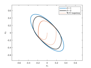
Figure 1: Approximate unit peak peak input reachable sets and worst case trajectory for the high damping system (37) .

The peak output of the worst case trajectory represents the lower bound for the $\ell_{1}$ norm Fig. 2 shows that value of this lower bound is $\mathbf{0.3097}$

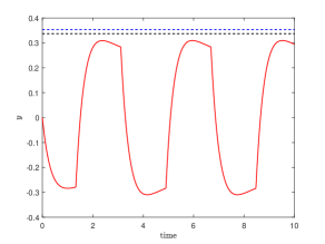
Figure 2: Red curve represents the ”Worst case” trajectory and the blue and black dotted lines are the star norm for $d=1$ and $d=2$ respectively for the high damping system (37)

VI-B System with low damping

Consider the following low damping system

$$\dot{x}=\begin{bmatrix}0&1\\ -0.5&-0.5\end{bmatrix}x+\begin{bmatrix}0\\ 1\end{bmatrix}u,\qquad y=\begin{bmatrix}1&1\end{bmatrix}x$$ (39)

The exact value of the $\ell_{1}$ norm is by calculating the integral $\int_{0}^{\infty}|Ce^{At}B|dt$ is $\mathbf{4.3069}$. The computations shows that the value of the star norm at ($d=2$), $\mathbf{4.5533}$, is less than the value of star norm obtained at ($d=1$), $\mathbf{4.63}$. In addition, Fig. 3 shows that the approximation of the unit peak input reachable set is less conservative when using the lifted system ($d=2$).

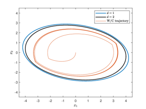
Figure 3: Approximate unit peak peak input reachable sets and worst case trajectory for low damping system (39) .

VI-C stiff system

Consider the following system

$$\dot{x}=\begin{bmatrix}-1&0\\ 0&-100\end{bmatrix}x+\begin{bmatrix}1\\ 100\end{bmatrix}u,\qquad y=\begin{bmatrix}1&-2\end{bmatrix}x$$ (40)

The exact value of the $\ell_{1}$ norm is $\mathbf{3.0412}$. The star norm computed when ($d=1$) is $\mathbf{10.4600}$ which is very conservative upper bound for the $\ell_{1}$ norm. However, the star norm computed using the lifted system is $\mathbf{5.7680}$ which shows the effectiveness of lifting the system to obtain better bounds. Also, Fig. 4 shows the significant effect of lifting in reducing the conservatism in reachable set approximations for system (40).

Figure 4: Approximate unit peak peak input reachable sets and worst case trajectory for stiff system (40) .

VII Alternative method to approximate $\ell_{1}$ norm

In this section, we introduce another method to get better and more accurate approximation for the $\ell_{1}$ norm which is $\int_{0}^{\infty}|Ce^{At}B|dt$. This integral is divided in two parts as:

$$\int_{0}^{\infty}|Ce^{At}B|dt=\int_{0}^{T_{0}}|Ce^{At}B|dt+\int_{T_{0}}^{\infty}\left|Ce^{At}B\right|dt$$ (41)

where $T_{0}>0$ is known, so the first term can be computed exactly. The second term is the $\ell_{1}$ norm of the following system:

$$\dot{z} =Az+e^{AT_{0}}Bu$$ (42)

$$y =Cz$$

An upper bound on the $\ell_{1}$ norm of system (42) can be approximated as the star norm where the system can be lifted to a higher order to obtain better approximation. Table I shows the upper bound of the $\ell_{1}$ norm of the low damping system (39) using different values of $T_{0}$. At each $T_{0}$, the first term in (41) is computed and the second term is approximated at $d=1$ and $d=2$ for the system (42).

TABLE I: $\ell_{1}$ norm approximation for system (39) [exact value is $4.3069$]

$T_{0}\text{(}Sec)$	Upper bound ($d=1$)	Upper bound ($d=2$)
2	4.5683	4.5304
5	4.4078	4.3981
10	4.3376	4.3332
20	4.3096	4.3091

This method provides more accurate approximations even for stiff system (40), The upper bound obtained by using $T_{0}=0.05\text{sec}$ and $d=2$ is $\mathbf{3.0424}$ which is very close to the exact value $\mathbf{3.0412}$

VIII CONCLUSIONS

This work demonstrates how the polynomial homogeneous Lyapunov function can be used to obtain better approximations for the LTI system’s star norm which is an upper bound for the system’s $\ell_{1}$ norm. We also demonstrated that the inescapable ellipsoids, approximations for the unit peak input reachable sets, generated using higher order Lyapunov functions is more accurate and less conservative that those produced by using quadratic Lyapunov functions. We tested that for three types of systems: systems with high damping, systems with low damping and stiff systems, to show the improvement of the reachable sets approximation. We only considered lifting the LTI system $d=2$. For $d>2$, the main difficulty is to transfer the inequality $u^{2}\leq 1$ in the original space to quadratic inequalities in the higher order space as in (28) for $d=2$. As a future work, we are working to develop new techniques to deal with this difficulty. Also, there are future opportunities to use homogeneous Lyapunov functions in robustness analysis and design better-performing controllers.

References

- [1] J. S. Shamma, “Nonlinear state feedback for optimal control,” Systems & control letters, vol. 21, no. 4, pp. 265–270, 1993.
- [2] J. Abedor, K. Nagpal, and K. Poolla, “A linear matrix inequality approach to peak-to-peak gain minimization,” International Journal of Robust and Nonlinear Control, vol. 6, no. 9-10, pp. 899–927, 1996.
- [3] E. M. Feron, “Linear matrix inequalities for the problem of absolute stability of control systems,” Ph.D. dissertation, Stanford University, 1994.
- [4] M. Vidyasagar, “Optimal rejection of persistent bounded disturbances,” IEEE Transactions on Automatic Control, vol. 31, no. 6, pp. 527–534, 1986.
- [5] S. Boyd and J. Doyle, “Comparison of peak and RMS gains for discrete-time systems,” Systems & control letters, vol. 9, no. 1, pp. 1–6, 1987.
- [6] V. Balakrishnan and S. Boyd, “On computing the worst-case peak gain of linear systems,” Systems & Control Letters, vol. 19, no. 4, pp. 265–269, 1992.
- [7] M. Dahleh and J. Pearson, “ optimal feedback controllers for discrete time systems,” IEEE Transactions on Automatic Control, vol. 32, no. 4, pp. 314–322, 1987.
- [8] ——, “ optimal compensators for continuous-time systems,” IEEE Transactions on Automatic Control, vol. 32, no. 10, pp. 889–895, 1987.
- [9] J. S. Shamma, “Optimization of the -induced norm under full state feedback,” IEEE Transactions on Automatic Control, vol. 41, no. 4, pp. 533–544, 1996.
- [10] M. Abate, C. Klett, S. Coogan, and E. Feron, “Lyapunov differential equation hierarchy and polynomial Lyapunov functions for switched linear systems,” in 2020 American Control Conference (ACC). IEEE, 2020, pp. 5322–5327.
- [11] ——, “Pointwise-in-time analysis and non-quadratic Lyapunov functions for linear time-varying systems,” in 2021 American Control Conference (ACC). IEEE, 2021, pp. 3550–3555.
- [12] B. J. Broxson, “The kronecker product,” 2006.
- [13] C. F. Van Loan, “The ubiquitous kronecker product,” Journal of computational and applied mathematics, vol. 123, no. 1-2, pp. 85–100, 2000.
- [14] R. A. Horn, R. A. Horn, and C. R. Johnson, Topics in matrix analysis. Cambridge university press, 1994.