Composable security for continuous variable quantum key distribution:
Trust levels and practical key rates in wired and wireless networks

Abstract

Continuous variable (CV) quantum key distribution (QKD) provides a powerful setting for secure quantum communications, thanks to the use of room-temperature off-the-shelf optical devices and the potential to reach much higher rates than the standard discrete-variable counterpart. In this work, we provide a general framework for studying the composable finite-size security of CV-QKD with Gaussian-modulated coherent-state protocols under various levels of trust for the loss and noise experienced by the parties. Our study considers both wired (i.e., fiber-based) and wireless (i.e., free-space) quantum communications. In the latter case, we show that high key rates are achievable for short-range optical wireless (LiFi) in secure quantum networks with both fixed and mobile devices. Finally, we extend our investigation to microwave wireless (WiFi) discussing security and feasibility of CV-QKD for very short-range applications.

I Introduction

Quantum key distribution (QKD) QKDreview enables the generation of secret keys between two or more authenticated parties by resorting to the fundamental laws of quantum mechanics. Its continuous variable (CV) version Cerf ; GG02 ; noswitch ; CVMDI ; RMP represents a very profitable setting and opportunity thanks to its more direct implementation in the current communication infrastructure and, most importantly, for its potential to approach the ultimate rate limits of quantum communication, as represented by the repeaterless PLOB bound QKDpaper . From an experimental point of view, we have been witnessing an increasing number of realizations closing the gap with the more traditional qubit-based implementations LeoCodes ; LeoEXP .

The most advanced protocols of CV-QKD are the Gaussian-modulated coherent-state protocols GG02 ; noswitch ; CVMDI . Not only they are very practical, but also enjoy the most advanced security proofs, accounting for finite-size effects (i.e., finite number of signal exchanges) and composability (so that each step of the protocol has an associated error which adds to an overall ‘epsilon’-security) QKDreview ; noteDalpha . Very recently, this level of security has been extended to the free-space setting FSpaper ; SATpaper , where we need to consider not only the presence of diffraction-induced loss Goodman ; Siegman ; svelto , atmospheric extinction Huffman and background thermal noise Miao ; BrussSAT , but also the effect of fading, as induced by pointing error and turbulence Vasy12 ; Esposito ; Yura73 ; Fante75 ; AndrewsBook ; Majumdar ; Hemani . The importance of studying fading and atmospheric effects in CV-QKD is an active area with increasing efforts put by the community at large (e.g. see Refs. refC1 ; refC1b ; refC2 ; refC2b ; PanosFading ; refC4 ; refC5 ; refC6 ; refC7 ; refC8 ; refC9 ; refC10 ).

While composable security is typically assessed against collective or coherent attacks, experiments may involve some additional (realistic) assumptions that elude this theory. For instance, these assumptions may concern some level of trusted noise in the setups (e.g., this is often the case for the electronic noise of the detector) or some realistic constraint on the eavesdropper, Eve (e.g., it may be considered to be passive in line-of-sight free-space implementations). For this reason, here we present the general theory to cover all these cases.

In fact, we consider various levels of trust for the receiver’s setup, starting from the traditional scenario where detector’s loss or noise are untrusted, meaning that Eve may perform a side-channel attack over the receiver besides attacking the main channel. Then, we consider the case where detector’s noise is trusted but not its loss, which corresponds to Eve collecting leakage from the receiver. Finally, we study the more trustful scenario where both detector’s loss and noise are considered to be trusted, so that Eve is excluded from side-channels to the receiver. We show how these assumptions can non-trivially increase the composable key rates of Gaussian-modulated CV-QKD protocols and tolerate higher dBs.

In our analysis, we then investigate the free-space setting, specifically for near-range wireless quantum communications at optical frequencies (LiFi). This scenario involves the presence of free-space diffraction and also fading effects, mainly due to pointing and tracking errors associated with the limited technology of the transmitter (while we can neglect turbulence at such distances). We consider communication with both fixed and mobile devices, assuming realistic parameters for indoor conditions and relatively-large field-of-views for the receivers. Security is studied under the various trusted models for the receiver’s detector and then including additional assumptions for Eve due to the line-of-sight configuration. Here too we show that key rates are remarkably increased as an effect of the realistic assumptions. More interestingly, we show that wireless high-rate CV-QKD is indeed feasible with mobile devices.

Finally, we consider wireless quantum communications at the microwave frequencies (WiFi) where both loss and thermal noise are very high. In this scenario, we consider a potential regime of parameters that enables very short-range quantum security, e.g., between contact-less devices within the range of a few centimeters.

The paper is organized as follows. In Sec. II, we provide a general framework for the composable security of CV-QKD, which also accounts for levels of trust in the loss and noise of the communication. In Sec. III, we consider near-range free-space quantum communications, first at optical frequencies (with fixed and mobile devices) and then at the microwaves. Sec. IV is for conclusions.

II General framework for composable security of CV-QKD

II.1 General description

Let us consider a Gaussian-modulated coherent-state protocol between Alice (transmitter) and Bob (receiver). Alice prepares a coherent state $\left|\alpha\right\rangle$ whose amplitude $\alpha$ is modulated according to a complex Gaussian distribution with zero mean and variance $\mu-1$. Assuming the notation of Ref. RMP , we may decompose the amplitude as $\alpha=(q+ip)/2$, where $x=q$ or $p$ represents the mean value of the generic quadrature operator $\hat{x}=\hat{q},\hat{p}$ where $[\hat{q},\hat{p}]=2i$. This generic quadrature can be written as $\hat{x}=\hat{x}_{0}+x$, where $\hat{x}_{0}$ is the vacuum noise associated with the bosonic mode and the real variable $x$ is a random Gaussian displacement with zero mean and variance

$$\sigma_{x}^{2}=\mu-1.$$ (1)

The coherent state is sent through a thermal-loss channel controlled by the eavesdropper, with transmissivity $\eta_{\text{ch}}$ and mean number of thermal photons $\bar{n}_{e}$. Equivalently, we may introduce the variance $\omega=2\bar{n}_{e}+1$ and the background thermal noise $\bar{n}_{B}$ defined by $\bar{n}_{e}=\bar{n}_{B}/(1-\eta_{\text{ch}})$, so $\bar{n}_{B}$ photons are added to the input signal. Bob’s setup is characterized by quantum efficiency $\eta_{\text{eff}}$ and extra noise variance $\nu_{\text{ex}}=2\bar{n}_{\text{ex}}$, where $\bar{n}_{\text{ex}}$ is an equivalent number of thermal photons generated by the imperfections in his receiver station (due to electronic noise, phase errors etc.)

From an energetic point of view, the initial mean photons at the transmitter $\bar{n}_{T}$ are attenuated by an overall factor $\tau=\eta_{\text{ch}}\eta_{\text{eff}}$ which can be seen as the total effective transmissivity of the extended channel between Alice and Bob. Thus, the total mean number of photons that are seen by the receiver’s detector is given by

$$\bar{n}_{R}=\tau\bar{n}_{T}+\bar{n},$$ (2)

where $\bar{n}$ is the total number of thermal photons due to the various sources of noise, given by

$$\bar{n}=\eta_{\text{eff}}\bar{n}_{B}+\bar{n}_{\text{ex}}.$$ (3)

See also Fig. 1 for a schematic of the overall scenario.

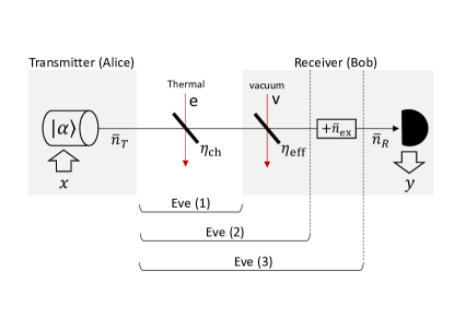
Figure 1: Quantum communication scenario between transmitter (Alice) and receiver (Bob) separated by a quantum channel with transmissivity $\eta_{\text{ch}}$ and thermal number $\bar{n}_{e}=\bar{n}_{B}/(1-\eta_{\text{ch}})$. Bob’s setup has quantum efficiency $\eta_{\text{eff}}$ and extra thermal photons $\bar{n}_{\text{ex}}$. The mean number of photons at the input ($\bar{n}_{T}$) and output ($\bar{n}_{R}$) follow Eq. (2), while the input classical variable ($x$) and the output one ($y$) follow Eq. (4). We also describe the various trust levels for the receiver. In the scenario “Eve (1)”, the eavesdropper is assumed to attack the external channel only. In the scenario “Eve (2)’, there is also a passive side-channel attack where the eavesdropper collects leakage from the receiver’s setup. Finally, in the scenario “Eve (3)”, we assume that the eavesdropper is also able to perform an active side-channel attack, so that the noise internal to the setup has to be considered untrusted.

Bob’s detection is either a randomly-switched homodyne, measuring $\hat{q}$ or $\hat{p}$ GG02 , or heterodyne, realizing the joint measurement of $\hat{q}$ and $\hat{p}$ noswitch . We may treat both cases compactly with the same formalism. In both protocols, Bob retrieves an outcome $y$ which corresponds to Alice’s input $x$. For the homodyne protocol, there is a single pair $(x,y)$ for each mode transmitted by Alice while, for the heterodyne protocol, there are two pairs of variables per mode (but affected by more noise).

The input-output relation for the total channel from the classical input $x$ to the output $y$ takes the form

$$y=\sqrt{\tau}x+z,$$ (4)

where $z$ is a noise variable. The latter is given by

$$z =\sqrt{\eta_{\text{eff}}(1-\eta_{\text{ch}})}\hat{x}_{e}+\sqrt{\tau}\hat{x}_{0}$$

$$+\sqrt{1-\eta_{\text{eff}}}\hat{x}_{v}+z_{\text{ex}}+z_{\text{det}},$$ (5)

where $\hat{x}_{e}$ denotes the quadrature of the thermal mode $e$, $\hat{x}_{v}$ is the quadrature associated with setup vacuum mode $v$ (quantum efficiency), $z_{\text{ex}}$ is a Gaussian variable with $\mathrm{var}(z_{\text{ex}})=2\bar{n}_{\text{ex}}$ accounting for the extra noise of the setup, and $z_{\text{det}}$ is an additional Gaussian variable with $\mathrm{var}(z_{\text{det}})=\nu_{\text{det}}-1$ where $\nu_{\text{det}}$ is the quantum duty (‘qu-duty’) associated with detection: $\nu_{\text{det}}=1$ for homodyne and $\nu_{\text{det}}=2$ for heterodyne. See also Fig. 1. In total the noise variable $z$ has variance

$$\sigma_{z}^{2}=2\bar{n}+\nu_{\text{det}}.$$ (6)

From the input-output relation of Eq. (4), we may compute Alice and Bob’s mutual information $I(x:y)$ which takes the same expression in direct reconciliation (where Bob infers $x$ from $y$) and reverse reconciliation (where Alice infers $y$ from $x$). In fact, from $\mathrm{var}(y)=\tau\sigma_{x}^{2}+\sigma_{z}^{2}$ and $\mathrm{var}(y|x)=\sigma_{z}^{2}$, we get

$$I(x:y)=\frac{\nu_{\text{det}}}{2}\log_{2}\left(1+\frac{\sigma_{x}^{2}}{\chi}\right),$$ (7)

where

$$\chi:=\frac{\sigma_{z}^{2}}{\tau}=\frac{2\bar{n}+\nu_{\text{det}}}{\tau}$$ (8)

is the equivalent noise. Clearly $I(x:y)$ can be specified to $I^{\text{hom}}$ (for homodyne) and $I^{\text{het}}$ (for heterodyne) by choosing the corresponding value for $\nu_{\text{det}}$.

Note that the equivalent noise can be re-written as

$$\chi=\xi_{\text{tot}}+\frac{\nu_{\text{det}}}{\tau},~{}\xi_{\text{tot}}:=\frac{2\bar{n}}{\tau},$$ (9)

where $\xi_{\text{tot}}$ defines the total excess noise. In turn, the total excess noise can be decomposed as

$$\xi_{\text{tot}} =\xi_{\text{ch}}+\xi_{\text{ex}},$$ (10)

$$\xi_{\text{ch}} :=\frac{2(\bar{n}-\bar{n}_{\text{ex}})}{\tau}=\frac{2\eta_{\text{eff}}\bar{n}_{B}}{\tau},$$ (11)

$$\xi_{\text{ex}} :=\frac{2\bar{n}_{\text{ex}}}{\tau},$$ (12)

where $\xi_{\text{ch}}$ is the excess noise of the external channel, i.e., related to the thermal background, while $\xi_{\text{ex}}$ is that associated with the extra noise in the setup.

Let us make an important remark on notation. The use of the excess noise $\xi_{\text{tot}}$ is typical in fiber-based communication channels, while the use of the equivalent number of thermal photons $\bar{n}$ is instead more appropriate for free-space channels. In general, the two notations are related by the formulas above and can be used interchangeably. In the following, we choose to work with $\bar{n}$ which is particularly convenient from the point of view of the finite-size estimators. However, for completeness, we also provide the corresponding formulations in terms of excess noise.

II.2 Local oscillator and setup noise

Before discussing security aspects, let us discuss the local oscillator (LO) and then clarify the main contributions to the setup noise. In terms of equivalent number of thermal photons, the setup noise can be decomposed as $\bar{n}_{\text{ex}}=\bar{n}_{\text{LO}}+\bar{n}_{\text{el}}+\bar{n}_{\text{other}}$, where $\bar{n}_{\text{LO}}$ is the mean number of thermal photons associated with the phase errors of the LO, $\bar{n}_{\text{el}}$ is the mean number of thermal photons generated by electronic noise, and $\bar{n}_{\text{other}}$ is any other uncharacterized but independent source of noise (here neglected). Similarly, we may write a corresponding decomposition in terms of excess noise $\xi_{\text{ex}}=\xi_{\text{LO}}+\xi_{\text{el}}+\xi_{\text{other}}$, which is obtained by using $\xi_{(...)}=2\bar{n}_{(...)}/\tau$.

II.2.1 Phase-locking via TLO or phase-reconstruction via LLO

LO is crucial in CV-QKD since it contains the phase information that allows the parties to exploit the two quadratures of the mode. In other words, Alice’s and Bob’s rotating reference frames need to be phase-locked so Bob can measure the incoming state in the same quadrature(s) chosen by Alice. To achieve this goal there are two techniques, the simplest solution of the transmitted LO (TLO) GG02 and the more challenging (but more secure) one of the local LO (LLO) LLO ; LLO2 ; LLO3 ; QKDreview .

With the TLO, the LO is generated by the transmitter and multiplexed in polarization with the signal mode/pulse. Both of them are sent through the channel and then de-multiplexed by the receiver before being interfered in the homodyne/heterodyne setup. With the LLO, bright reference pulses are regularly interleaved with the signal pulses (time multiplexing). At the receiver, both the signals and the references are measured with an independent local LO. From the references, Bob is able to track Alice’s rotating frame and, using this phase information, he suitably rotates the outcomes obtained from the signals in the phase space.

Note that both TLO and LLO require to employ half of the total pulses for phase locking or reconstruction. When we explicitly consider a clock $C$ for the system (pulses per second), the LLO involves an extra factor $1/2$ in front of the final key rate, unless this is compensated by using both the polarizations for the signal transmissions (not possible for the TLO).

II.2.2 Contributions to setup noise

From the point of view of the setup noise, we need to account for phase errors introduced by an imperfect LO. In TLO this is negligible ($\bar{n}_{\text{TLO}}\simeq 0$), while for the LLO it is non-trivial. In fact, assume that signal and reference pulses are generated with an average linewidth $l_{\text{W}}=(l_{\text{W}}^{\text{signal}}+l_{\text{W}}^{\text{LO}})/2$. Then, for input classical modulation $\sigma_{x}^{2}$ and transmissivity $\tau$, we may write FSpaper

$$\bar{n}_{\text{LLO}}\simeq\Theta_{\text{ph}}\tau,~{}\Theta_{\text{ph}}:=\pi\sigma_{x}^{2}C^{-1}l_{\text{W}}.$$ (13)

This contribution can equivalently be written as excess noise $\xi_{\text{LLO}}=2\bar{n}_{\text{LLO}}/\tau$, according to Eq. (12). For a cw-laser $l_{\text{W}}\simeq 1.6$ KHz, a clock $C=5~{}$MHz and a typical modulation $\sigma_{x}^{2}=9$ (i.e., $\mu=10$) one has $\xi_{\text{LLO}}\simeq 0.018$.

While the LLO introduces phase errors, it may actually be better when we consider the impact of electronic noise. The latter can be described by a variance $\nu_{\text{el}}$ or an equivalent number of photons $\bar{n}_{\text{el}}=\nu_{\text{el}}/2$. Its value depends on the frequency of the light $\nu$, features of the homodyne/heterodyne detector, such as its noise equivalent power (NEP) and the bandwidth $W$, as well as features of the LO, such as its power at detection $P_{\text{LO}}^{\text{det}}$ and the duration of its pulses $\Delta t_{\text{LO}}$. In fact, we may write

$$\bar{n}_{\text{el}}=\frac{\nu_{\text{det}}\mathrm{NEP}^{2}W\Delta t_{\text{LO}}}{2h\nu P_{\text{LO}}^{\text{det}}}.$$ (14)

In the case of a TLO, one has $P_{\text{LO}}^{\text{det}}=\tau P_{\text{LO}}$, where $P_{\text{LO}}$ is the LO initial power at the transmitter. For an LLO, we instead have $P_{\text{LO}}^{\text{det}}=P_{\text{LO}}$. Thus, by setting

$$\Theta_{\text{el}}:=\frac{\nu_{\text{det}}\mathrm{NEP}^{2}W\Delta t_{\text{LO}}}{2h\nu P_{\text{LO}}},$$ (15)

we may write

$$\bar{n}_{\text{el}}^{\text{TLO}}=\frac{\Theta_{\text{el}}}{\tau},~{}\bar{n}_{\text{el}}^{\text{LLO}}=\Theta_{\text{el}},$$ (16)

so the formulas for the total setup noise are

$$\bar{n}_{\text{ex}}^{\text{TLO}}\simeq\frac{\Theta_{\text{el}}}{\tau},~{}\bar{n}_{\text{ex}}^{\text{LLO}}\simeq\Theta_{\text{el}}+\Theta_{\text{ph}}\tau.$$ (17)

These formulas are in terms of equivalent number of thermal photons and they have corresponding expressions in terms of setup excess noise by using $\xi_{\text{ex}}=2\bar{n}_{\text{ex}}/\tau$.

Above we can see the different monotonicity of the setup noise with respect to $\tau$, between TLO and LLO. Assume $\lambda=800~{}$nm and $W=100~{}$MHz, so we have signal pulses of duration $\Delta t=10~{}$ns and LO pulses of duration $\Delta t_{\text{LO}}=10~{}$ns. For this bandwidth, we can assume the good value $\mathrm{NEP}=6~{}$pW/$\sqrt{\text{Hz}}$. Then, assuming $P_{\text{LO}}=100~{}$mW, we get $\Theta_{\text{el}}\simeq 1.45\times 10^{-3}$ for heterodyne detection ($\nu_{\text{det}}=2$). For the LLO this value remains low, while for the TLO it is rescaled by $1/\tau$, which means that it may become large at long distances. See also Fig. 2 for a comparison.

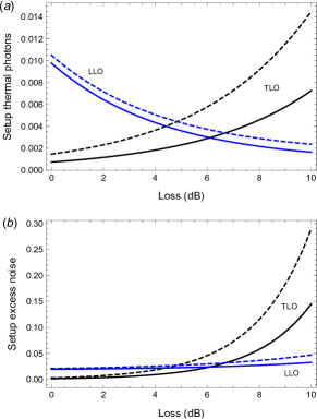
Figure 2: Setup noise as a function of the total transmissivity $\tau$ expressed in decibels. (a) We plot the equivalent number of thermal photons $\bar{n}_{\text{ex}}$ associated with the setup noise, for the TLO (black lines) and the LLO (blue lines), considering the homodyne protocol (solid lines) and the heterodyne protocol (dashed lines). (b) As in (a) but we plot the setup excess noise $\xi_{\text{ex}}$. Parameters are chosen as in the text. See Eq. (17).

II.3 Trust levels

Once we have clarified the main sources of noise in the communication scenario, we can go ahead and identify different levels of trust on the basis of different assumptions for the eavesdropper (Eve). The basic model is to assume that Eve’s action is restricted to the outside channel. In this strategy, she inserts her photons in the thermal background and stores all the photons which are not collected by the receiver. However, she is assumed not to monitor or control the receiver’s setup. This is the scenario where loss and noise are considered to be trusted in the receiver. See also Eve (1) in Fig. 1. In this case, Eve’s collective Gaussian attack is represented by a purification of the environmental beam-splitter of transmissivity $\eta_{\text{ch}}$, where the injected $\bar{n}_{e}^{(1)}=\bar{n}_{B}(1-\eta_{\text{ch}})^{-1}$ thermal photons are to be considered part of a two-mode squeezed vacuum (TMSV) state in Eve’s hands collectiveG .

More generally, we can assume that Eve is able to detect the leakage from setups refB1 ; refB2 ; refB3 . Here we consider this potential problem for the receiver’s setup, so that the fraction $1-\eta_{\text{eff}}$ of the photons missed by the detection is stored by Eve and becomes part of her attack. On the other hand, we may assume that Eve is not able to actively tamper with the receiver, i.e., she does not control the noise internal to the setup, which may therefore be considered as trusted (this is a reasonable assumption which is often made by experimentalists for the electronic noise of the detector). We call this scenario the trusted-noise model for the receiver. See Eve (2) in Fig. 1. In this case, the efficiency $\eta_{\text{eff}}$ becomes part of Eve’s environmental beam-splitter, which now has total transmissivity $\tau=\eta_{\text{ch}}\eta_{\text{eff}}$ and injects $\bar{n}_{e}^{(2)}=\eta_{\text{eff}}\bar{n}_{B}(1-\tau)^{-1}$ thermal photons.

Finally, there is the worst-case scenario where no imperfection in the receiver setup is trusted. In fact, the most pessimistic assumption is that Eve can also potentially control the extra photons in the setup $\bar{n}_{\text{ex}}$ besides collecting its leakage. See also Eve (3) in Fig. 1. In this case, the extra photons become part of Eve’s environment. In other words, the entire channel from the transmitter to the final (ideal) detection is dilated into a single beam-splitter with transmissivity $\tau=\eta_{\text{ch}}\eta_{\text{eff}}$ and injecting $\bar{n}_{e}^{(3)}=\bar{n}(1-\tau)^{-1}$ thermal photons.

Clearly the security increases from the completely trusted receiver [Eve (1)] to the worst-case scenario [Eve (3)]. Similarly, the key rate will decrease, because more degrees of freedom would go under Eve’s control. For this reason, the worst-case scenario provides a lower bound for all the others. Also note that the worst-case scenario progressively collapses in the lower levels if we assume $\bar{n}_{\text{ex}}=0$ and then $\eta_{\text{eff}}=1$. Also note that, in general, one  may consider hybrid situations between Eve (2) and Eve (3), where the setup noise $\bar{n}_{\text{ex}}$ is partly trusted ($\bar{n}_{\text{ex}}^{\text{tr}}$) and partly untrusted ($\bar{n}_{\text{ex}}^{\text{unt}}$). This is included by writing $\bar{n}_{\text{ex}}^{\text{unt}}=\eta_{\text{eff}}\bar{n}_{B}^{\text{unt}}$ and increasing the background $\bar{n}_{B}\rightarrow\bar{n}_{B}+\bar{n}_{B}^{\text{unt}}$.

II.4 Asymptotic key rates

It is convenient to start by studying the security of the protocol with the intermediate assumption of a trusted-noise detector as in Fig. 3, where the setup noise is considered to be trusted, i.e., not coming from Eve’s attack [cf. Eve (2) in Fig. 1]. Then, we analyze the key rate in the most optimistic case where also the setup loss is considered to be trusted. Finally, we compare the formulas with the worst-case scenario, where all noise is considered to be untrusted [cf. Eve (3) in Fig. 1]. The latter represents the case analyzed in Ref. FSpaper .

II.4.1 Asymptotic key rate with a trusted-noise detector

Consider the trusted-noise detector which corresponds to the dilated scenario in Fig. 3. Here the total transmissivity is $\tau=\eta_{\text{ch}}\eta_{\text{eff}}$ and the injected thermal noise is given by $\bar{n}_{e}^{(2)}=\eta_{\text{eff}}\bar{n}_{B}(1-\tau)^{-1}$. In order to compute the asymptotic secret key rate in reverse reconciliation, we consider Bob and Eve’s joint covariance matrix (CM). Let us define the basic block matrices $\mathbf{I}:=\mathrm{diag}(1,1)$ and $\mathbf{Z}:=\mathrm{diag}(1,-1)$. Then, the joint CM is given by

$$\mathbf{V}_{BEE^{\prime}}=\left(\begin{array}[c]{cc}b\mathbf{I}&\mathbf{C}\\ \mathbf{C}^{T}&\mathbf{V}_{EE^{\prime}}\end{array}\right),$$ (18)

where Eve’s reduced CM $\mathbf{V}_{EE^{\prime}}$ and the cross-correlation block $\mathbf{C}$ take the forms

$$\mathbf{V}_{EE^{\prime}}=\left(\begin{array}[c]{cc}\phi\mathbf{I}&\psi\mathbf{Z}\\ \psi\mathbf{Z}&\omega\mathbf{I}\end{array}\right),~{}\mathbf{C}=\left(\begin{array}[c]{cc}\theta\mathbf{I}&\gamma\mathbf{Z}\end{array}\right),$$ (19)

where we have set

$$\omega =2\bar{n}_{e}^{(2)}+1=\frac{2\eta_{\text{eff}}\bar{n}_{B}}{1-\tau}+1=\frac{\tau\xi_{\text{ch}}}{1-\tau}+1,$$ (20)

$$b =\tau(\mu-1)+2\bar{n}+1=\tau(\mu-1)+\tau\xi_{\text{tot}}+1,$$ (21)

$$\gamma =\sqrt{(1-\tau)(\omega^{2}-1)},~{}\theta=\sqrt{\tau(1-\tau)}(\omega-\mu),$$ (22)

$$\psi =\sqrt{\tau(\omega^{2}-1)},~{}\phi=\tau\omega+(1-\tau)\mu.$$ (23)

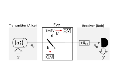
Figure 3: Eve’s collective attack under the assumption of trusted noise in the receiver’s setup, i.e., Eve (2) in Fig. 1.

In the homodyne protocol, Eve’s conditional CM on Bob’s outcome $y$ is given by RMP ; GaeCM ; GaeCM2

$$\mathbf{V}_{EE^{\prime}|B}^{\text{hom}}=\mathbf{V}_{EE^{\prime}}-b^{-1}\mathbf{C}^{T}\bm{\Pi}\mathbf{C},$$ (24)

where $\bm{\Pi}:=\mathrm{diag}(1,0)$. In the heterodyne protocol, we have instead the following conditional CM RMP ; GaeCM ; GaeCM2

$$\mathbf{V}_{EE^{\prime}|B}^{\text{het}}=\mathbf{V}_{EE^{\prime}}-(b+1)^{-1}\mathbf{C}^{T}\mathbf{C}.$$ (25)

Call $\{\nu_{\pm}\}$ the symplectic spectrum of Eve’s CM $\mathbf{V}_{EE^{\prime}}$. Then, call $\{\nu_{\pm}^{\text{hom}}\}$ and $\{\nu_{\pm}^{\text{het}}\}$ the symplectic spectra of Eve’s conditional CMs $\mathbf{V}_{EE^{\prime}|B}^{\text{hom}}$ and $\mathbf{V}_{EE^{\prime}|B}^{\text{het}}$, respectively. Then, we may compute Eve’s Holevo information for both protocols, as

$$\chi^{\text{hom}}(\mathbf{E} :y)=\sum\limits_{k=\pm}\left[H(\nu_{k})-H(\nu_{k}^{\text{hom}})\right],$$ (26)

$$\chi^{\text{het}}(\mathbf{E} :y)=\sum\limits_{k=\pm}\left[H(\nu_{k})-H(\nu_{k}^{\text{het}})\right],$$ (27)

where $\mathbf{E}=EE^{\prime}$ and $H(x)$ is the entropic function

$$H(x):=\frac{x+1}{2}\log_{2}\frac{x+1}{2}-\frac{x-1}{2}\log_{2}\frac{x-1}{2}.$$ (28)

For a realistic reconciliation efficiency $\beta\in[0,1]$, accounting for the fact that data-processing may not reach the Shannon limit, we write the asymptotic key rate

$$R_{\text{asy}}^{(2)}(\tau,\bar{n},\bar{n}_{B})=\beta I(x:y)_{\tau,\bar{n}}-\chi(\mathbf{E}:y)_{\tau,\bar{n},\bar{n}_{B}},$$ (29)

where the explicit expressions for the homodyne protocol GG02 and the heterodyne protocol noswitch derive from the corresponding expressions for the mutual information [cf. Eq. (7)] and the Holevo bound [cf. Eqs. (26) and (27)].

It is clear that, in a practical setting, the parties do not know all the parameters entering the rate in Eq. (29), so they need to resort to suitable procedures of parameter estimation. It is acceptable to assume that Alice controls/knows the signal modulation $\mu$, while Bob monitors/knows the quantum efficiency $\eta_{\text{eff}}$. The channel parameters $\tau$ and $\bar{n}$ need to be estimated. In general, the setup noise $\bar{n}_{\text{ex}}$ depends on the total transmissivity $\tau$. For this reason, $\bar{n}_{\text{ex}}$ too needs to be estimated by the parties. The estimates of $\bar{n}$ and $\bar{n}_{\text{ex}}$ then provide the value of $\bar{n}_{B}$.

II.4.2 Asymptotic key rate with a trusted-loss and trusted-noise detector

Here we consider the best possible scenario for Alice and Bob, which is the assumption of Eve (1) in Fig. 1. Not only the setup noise is trusted but also the loss of the setup into the external environment is considered to be trusted (i.e., we assume Eve is not collecting the leakage from the setup). The asymptotic key rate can be found by a simple modification of the previous derivation.

From the point of view of Alice and Bob, the mutual information is clearly the same. For Eve instead, the effective beam splitter used in her attack has now transmissivity $\eta_{\text{ch}}$ and input thermal noise $\bar{n}_{e}^{(1)}=\bar{n}_{B}(1-\eta_{\text{ch}})^{-1}$. It is easy to check that we need to use the CM in Eq. (19) with the replacements

$$\omega =2\bar{n}_{e}^{(1)}+1=\frac{2\bar{n}_{B}}{1-\eta_{\text{ch}}}+1=\frac{\eta_{\text{ch}}\xi_{\text{ch}}}{1-\eta_{\text{ch}}}+1,$$ (30)

$$\gamma =\sqrt{\eta_{\text{eff}}(1-\eta_{\text{ch}})(\omega^{2}-1)},$$ (31)

$$\theta =\sqrt{\tau(1-\eta_{\text{ch}})}(\omega-\mu),$$ (32)

$$\psi =\sqrt{\eta_{\text{ch}}(\omega^{2}-1)},~{}\phi=\eta_{\text{ch}}\omega+(1-\eta_{\text{ch}})\mu,$$ (33)

while parameter $b$ is the same as in Eq. (21).

The next steps are as before. One computes the symplectic spectrum $\{\nu_{\pm}\}$ of the CM $\mathbf{V}_{EE^{\prime}}$ and those, $\{\nu_{\pm}^{\text{hom}}\}$ and $\{\nu_{\pm}^{\text{het}}\}$, of the conditional CMs $\mathbf{V}_{EE^{\prime}|B}^{\text{hom}}$ and $\mathbf{V}_{EE^{\prime}|B}^{\text{het}}$. These eigenvalues are then replaced in Eqs. (26) and (27). In this way, we get the corresponding asymptotic key rates $R_{\text{asy}}^{(1)}(\tau,\bar{n},\bar{n}_{B})$ following the formula in Eq. (29). Parameters need to be estimated in the same way as explained in the previous subsection.

II.4.3 Asymptotic key rate with untrusted detector

In the worst-case scenario of untrusted noise [cf. Eve (3) in Fig. 1], the entire channel is dilated into a single beam splitter with transmissivity $\tau=\eta_{\text{ch}}\eta_{\text{eff}}$, where Eve injects $\bar{n}_{e}^{(3)}=\bar{n}(1-\tau)^{-1}$ thermal photons. Setup noise $\bar{n}_{\text{ex}}$ becomes part of Eve’s attack, so all excess noise is now considered to be untrusted. From the point of view of the asymptotic key rate, it is sufficient to replace $\eta_{\text{eff}}\bar{n}_{B}=\bar{n}-\bar{n}_{\text{ex}}\rightarrow\bar{n}$ in the expression of Eve’s variance $\omega$ in Eq. (20), with implicit modifications for the other elements of the CM. More precisely, it is sufficient to set

$$\omega=2\bar{n}_{e}^{(3)}+1=\frac{2\bar{n}}{1-\tau}+1=\frac{\tau\xi_{\text{tot}}}{1-\tau}+1.$$ (34)

Alternatively, we can exploit the entanglement-based representation of the protocol according to which Alice’s Gaussian-modulated coherent states are realized by heterodyning mode $A$ of a TMSV state RMP with CM

$$\mathbf{V}_{AA^{\prime}}=\left(\begin{array}[c]{cc}\mu\mathbf{I}&\sqrt{\mu^{2}-1}\mathbf{Z}\\ \sqrt{\mu^{2}-1}\mathbf{Z}&\mu\mathbf{I}\end{array}\right).$$ (35)

After the thermal-loss channel with total transmissivity $\tau$, Alice and Bob’s shared Gaussian state $\rho_{AB}$ has CM

$$\mathbf{V}_{AB}=\left(\begin{array}[c]{cc}\mu\mathbf{I}&\sqrt{\tau(\mu^{2}-1)}\mathbf{Z}\\ \sqrt{\tau(\mu^{2}-1)}\mathbf{Z}&b\mathbf{I}\end{array}\right).$$ (36)

Eve is assumed to hold the purification of $\rho_{AB}$, so the total state $\rho_{AB\mathbf{E}}$ of Alice, Bob and Eve is pure. This means that $S(\mathbf{E})=S(AB)$, where $S(Q)$ denotes the von Neumann entropy computed over the state $\rho_{Q}$ of system $Q$. Then, because homodyne/heterodyne is a rank-1 measurement (projecting pure states in pure states), we have that $\rho_{A\mathbf{E}|y}$ is pure, which implies the equality of the conditional entropies $S(\mathbf{E}|y)=S(A|y)$. As a result, Eve’s Holevo bound is simply given by

$$\chi(\mathbf{E}:y):=S(\mathbf{E})-S(\mathbf{E}|y)=S(AB)-S(A|y).$$ (37)

Thus, we may compute $\chi(\mathbf{E}:y)$ using Alice and Bob’s CM $\mathbf{V}_{AB}$ with symplectic eigenvalues $\nu_{\pm}^{\prime}$. It is easy to find FSpaper

$$\chi^{\text{hom}}(\mathbf{E} :y)=H(\nu_{+}^{\prime})+H(\nu_{-}^{\prime})-H\left[\sqrt{\mu^{2}-\frac{\mu\tau(\mu^{2}-1)}{b}}\right],$$ (38)

$$\chi^{\text{het}}(\mathbf{E} :y)=H(\nu_{+}^{\prime})+H(\nu_{-}^{\prime})-H\left[\mu-\frac{\tau(\mu^{2}-1)}{b+1}\right],$$ (39)

where $b$ is given in Eq. (21).

Using these expressions and the mutual information of Eq. (7), we write

$$R_{\text{asy}}^{(3)}(\tau,\bar{n})=\beta I(x:y)_{\tau,\bar{n}}-\chi(\mathbf{E}:y)_{\tau,\bar{n}}.$$ (40)

Note that the parties only need to estimate the extended-channel parameters $\tau$ and $\bar{n}$. As we see below these estimators are built up to some error probability $\varepsilon_{\text{pe}}$.

II.5 Parameter estimation

As mentioned in the previous section, Alice and Bob need to estimate some of the parameters. Even if they control the values of the input Gaussian modulation $\mu$ and they can calibrate the output quantum efficiency $\eta_{\text{eff}}$, they still need to estimate the various channel’s parameters and the setup noise $\bar{n}_{\text{ex}}$. The procedure has some differences depending if we consider a trusted or untrusted model for the receiver. For a trusted-noise detector [Eve (2)] and a fully-trusted detector [Eve (1)], Alice and Bob need to estimate $\tau$, $\bar{n}$ and $\bar{n}_{B}$ (via $\bar{n}_{\text{ex}}$). For the untrusted detector [Eve (3)], they only need to estimate $\tau$ and $\bar{n}$, since the two thermal contributions $\bar{n}_{B}$ and $\bar{n}_{\text{ex}}$ are both considered to be untrusted (and therefore merged into a single parameter).

We therefore consider two basic independent estimators $\hat{\tau}$ and $\widehat{\bar{n}}$, for $\tau$ and $\bar{n}$. Then, in the trusted scenarios [Eve (1) and (2)], we also require the use of additional estimators, which can be derived from the basic ones. To estimate the parameters, Alice and Bob randomly and jointly choose $m$ of the $N$ distributed signals, and publicly disclose the corresponding $m_{p}:=\nu_{\text{det}}m$ pairs of values $\{x_{i},y_{i}\}_{i=1}^{m_{p}}$. These are $m$ pairs for the homodyne protocol and $2m$ pairs for the heterodyne protocol. Under the standard assumption of a collective (entangling-cloner) Gaussian attack, these pairs are independent and identically distributed Gaussian variables, related by Eq. (4).

From the pairs, they build the estimator $\hat{T}$ of the square-root transmissivity $T:=\sqrt{\tau}$, i.e.,

$$\hat{T}=\frac{\sum_{i=1}^{m_{p}}x_{i}y_{i}}{\sum_{i=1}^{m_{p}}x_{i}^{2}},$$ (41)

and the estimator $\widehat{\sigma_{z}^{2}}$ of the noise variance $\sigma_{z}^{2}$, i.e.,

$$\widehat{\sigma_{z}^{2}}=\frac{1}{m_{p}}\sum_{i=1}^{m_{p}}(y_{i}-\hat{T}x_{i})^{2}.$$ (42)

From these, we can derive the two basic estimators

$$\hat{\tau}:=\hat{T}^{2},~{}\widehat{\bar{n}}:=\frac{\widehat{\sigma_{z}^{2}}-\nu_{\text{det}}}{2}.$$ (43)

For a confidence parameter $w$, we then define and compute the worst-case estimators NoteEstimator

$$\tau^{\prime} :=\hat{\tau}-w\sqrt{\mathrm{var}(\hat{\tau})}\simeq\tau-2w\sqrt{\frac{2\tau^{2}+\tau\sigma_{z}^{2}/\sigma_{x}^{2}}{m_{p}}},$$ (44)

$$\bar{n}^{\prime} :=\widehat{\bar{n}}+w\sqrt{\mathrm{var}(\widehat{\bar{n}})}\simeq\bar{n}+w\frac{\sigma_{z}^{2}}{\sqrt{2m_{p}}}.$$ (45)

Each of these estimators bounds the corresponding actual value, $\tau$ and $\bar{n}$, up to an error probability $\varepsilon_{\text{pe}}$ if we take

$$w=\sqrt{2}\operatorname{erf}^{-1}(1-2\varepsilon_{\text{pe}}),$$ (46)

or, in case of low values ($\varepsilon_{\text{pe}}\leq 10^{-17}$), if we take

$$w=\sqrt{2\ln(1/\varepsilon_{\text{pe}})}.$$ (47)

As a result the total error probability associated with parameter estimation is $\simeq 2\varepsilon_{\text{pe}}$. See Ref. FSpaper for more technical details on these derivations, which exploit tools from Ref. UsenkoFinite and involves suitable tail bounds TailBound ; Kolar .

For the trusted-detector scenarios, we need to provide the best-case estimator of $\bar{n}_{\text{ex}}$, which automatically allows us to derive the worst-case estimator of $\bar{n}_{B}$. From the analytical expressions in Eq. (17), we see that we need to account for the different behavior of $\bar{n}_{\text{ex}}$ in terms of the transmissivity $\tau$, which requires both the use of a worst-case estimator $\tau^{\prime}$ and that of a best-case estimator $\tau^{\prime\prime}:=\hat{\tau}+w\sqrt{\mathrm{var}(\hat{\tau})}$. In other words, we have

$$\bar{n}_{\text{ex}}^{\text{TLO}} \gtrsim\bar{n}_{\text{ex,bc}}^{\text{TLO}}:=\frac{\Theta_{\text{el}}}{\tau^{\prime\prime}},$$ (48)

$$\bar{n}_{\text{ex}}^{\text{LLO}} \gtrsim\bar{n}_{\text{ex,bc}}^{\text{LLO}}:=\Theta_{\text{el}}+\Theta_{\text{ph}}\tau^{\prime}.$$ (49)

Correspondingly, we have the following worst-case estimator for the background thermal noise

$$\bar{n}_{B}\lesssim\bar{n}_{B}^{\prime}:=\frac{\bar{n}^{\prime}-\bar{n}_{\text{ex,bc}}}{\eta_{\text{eff}}}.$$ (50)

We can now compute the values of the asymptotic key rates affected by parameter estimation. For the various scenarios, these are given by

$$R_{\text{asy}}^{(1,2)}(\tau,\bar{n},\bar{n}_{B}) \rightarrow\frac{n}{N}R_{\text{asy}}^{(1,2)}(\tau^{\prime},\bar{n}^{\prime},\bar{n}_{B}^{\prime}),$$ (51)

$$R_{\text{asy}}^{(3)}(\tau,\bar{n}) \rightarrow\frac{n}{N}R_{\text{asy}}^{(3)}(\tau^{\prime},\bar{n}^{\prime}),$$ (52)

where $n=N-m$ is the number of signals left for key generation (after $m$ are discarded for parameter estimation). These key rates are correct up to an error $\simeq 2\varepsilon_{\text{pe}}$.

As a final remark, notice that the total excess noise $\xi_{\text{tot}}$ can be estimated by using $\hat{\tau}$ and $\widehat{\bar{n}}$ via Eq. (9) and therefore worst-case estimated by using $\tau^{\prime}$ and $\bar{n}^{\prime}$, i.e.,

$$\xi_{\text{tot}}\lesssim\xi_{\text{tot}}^{\prime}:=\frac{2\bar{n}^{\prime}}{\tau^{\prime}}.$$ (53)

Similarly, the channel excess noise $\xi_{\text{ch}}$ can be worst-case estimated by combining Eq. (11) with $\tau^{\prime}$ and $\bar{n}_{B}^{\prime}$, i.e.,

$$\xi_{\text{ch}}\lesssim\xi_{\text{ch}}^{\prime}:=\frac{2\eta_{\text{eff}}\bar{n}_{B}^{\prime}}{\tau^{\prime}}.$$ (54)

II.6 Composable finite-size key rates

After parameter estimation, each block of size $N$ provides $n$ signals to be processed into a shared key via error correction and privacy amplification. Given a block, this is successfully error-corrected with probability $p_{\text{ec}}$ (or failure probability $\mathrm{FER}=1-p_{\text{ec}}$ known as ‘frame error rate’). The value of $p_{\text{ec}}$ depends on the signal-to-noise ratio, the target reconciliation efficiency $\beta$, and the $\varepsilon$-correctness $\varepsilon_{\text{cor}}$, the latter bounding the probability that Alice’s and Bob’s local strings are different after error correction and successful verification of their hashes.

On average $np_{\text{ec}}$ signals per block are promoted to privacy amplification. This final step is implemented with an associated $\varepsilon$-secrecy $\varepsilon_{\text{sec}}$, the latter bounding the distance between the final key and an ideal key that is completely uncorrelated from Eve. In turn, the $\varepsilon$-secrecy is technically decomposed as $\varepsilon_{\text{sec}}=\varepsilon_{\text{s}}+\varepsilon_{\text{h}}$, where $\varepsilon_{\text{s}}$ is a smoothing parameter and $\varepsilon_{\text{h}}$ is a hashing parameter.

Overall, the final composable key rate of the protocol takes the form FSpaper

$$R\geq\frac{np_{\text{ec}}}{N}\left(R_{\text{pe}}^{(k)}-\frac{\Delta_{\text{aep}}}{\sqrt{n}}+\frac{\Theta}{n}\right),$$ (55)

where $R_{\text{pe}}^{(k)}$ depends on the receiver model

$$R_{\text{pe}}^{(1,2)}=R_{\text{asy}}^{(1,2)}(\tau^{\prime},\bar{n}^{\prime},\bar{n}_{B}^{\prime}),~{}~{}R_{\text{pe}}^{(3)}=R_{\text{asy}}^{(3)}(\tau^{\prime},\bar{n}^{\prime}),$$ (56)

and the extra finite-size terms are equal to

$$\Delta_{\text{aep}}=4\log_{2}\left(2\sqrt{d}+1\right)\sqrt{\log_{2}\left(\frac{18}{p_{\text{ec}}^{2}\varepsilon_{\text{s}}^{4}}\right)},$$ (57)

$$\Theta=\log_{2}[p_{\text{ec}}(1-\varepsilon_{\text{s}}^{2}/3)]+2\log_{2}\sqrt{2}\varepsilon_{\text{h}}.$$ (58)

Here the parameter $d$ is the size of Alice’s and Bob’s effective alphabet after analog-to-digital conversion of their continuous variables $x$ and $y$ ($d=2^{5}=32$ for a $5$-bit discretization). This rate refers to security against collective Gaussian attacks with total epsilon security FSpaper

$$\varepsilon=2p_{\text{ec}}\varepsilon_{\text{pe}}+\varepsilon_{\text{cor}}+\varepsilon_{\text{sec}}.$$ (59)

II.6.1 Improved pre-factor

Note that the prefactor $\log_{2}(2\sqrt{d}+1)$ in the AEP term in Eq. (57) can be tightened into $\log_{2}(\sqrt{d}+2)$. In general, according to Theorem 6.4 and Corollary 6.5 of Ref. TomaThesis , one can lower-bound the conditional smooth min-entropy $H_{\min}^{\delta}(y^{n}|\mathbf{E}^{n})$ associated with the $n$-use classical-quantum state $\rho_{y\mathbf{E}}^{\otimes n}$ shared between Bob (classical system $y$) and Eve (quantum system $\mathbf{E}$). This is done by using the conditional entropy between the single-use systems ($y$ and $\mathbf{E}$) up to a penalty, i.e., we may write TomaThesis ; TomaBook

$$H_{\min}^{\delta}(y^{n}|\mathbf{E}^{n})_{\rho^{\otimes n}}\geq nH(y|\mathbf{E})_{\rho}+\sqrt{n}\Delta_{\text{aep}}(\delta),$$ (60)

where

$$\Delta_{\text{aep}}(\delta) =4(\log_{2}v)\sqrt{-\log_{2}(1-\sqrt{1-\delta^{2}})}$$

$$\simeq 4(\log_{2}v)\sqrt{\log_{2}(2/\delta^{2})}$$ (61)

$$v \leq\sqrt{2^{-H_{\min}(y|\mathbf{E})}}+\sqrt{2^{H_{\max}(y|\mathbf{E})}}+1,$$ (62)

with $v$ being bounded using min- and max-entropies. Recall that the min- and max-entropies can be negative in general, but their absolute values must be $\leq\log_{2}d$, with $d$ being the size of Bob’s alphabet (e.g., this easily follows from Ref. (TomaBook, , Lemma 5.2)). This implies the bound $v\leq 2\sqrt{d}+1$, which leads to the prefactor used in Eq. (57). See Ref. (FSpaper, , Appendix G) for details on how to connect the key rate with the conditional smooth min-entropy and simplify derivations via the AEP term.

However, it is worth noting that, for a classical-quantum state $\rho_{y\mathbf{E}}$, the conditional min-entropy is non-negative, i.e., $H_{\min}(y|\mathbf{E})\geq 0$. This is a property that can be shown, more generally, for separable states. In fact, starting from the definition of conditional min-entropy for a generic state $\rho_{AB}$ of two quantum systems $A$ and $B$ (TomaThesis, , Def. 4.1), we can write the lower bound

$$H_{\min}(A|B)_{\rho}\geq\tilde{H}:=\sup\{\lambda\in\mathbb{R}:\rho_{AB}\leq 2^{-\lambda}I_{A}\otimes\rho_{B}\}.$$ (63)

For separable $\rho_{AB}$, one may write (TomaBook, , Lemma 5.2)

$$\rho_{AB}=\sum_{k}p_{k}\theta_{A}^{k}\otimes\rho_{B}^{k}\leq\sum_{k}p_{k}I_{A}\otimes\rho_{B}^{k}=I_{A}\otimes\rho_{B},$$ (64)

which leads to $\tilde{H}\geq 0$, since we are left to find the maximum value of $\lambda$ such that

$$\rho_{AB}\leq I_{A}\otimes\rho_{B},~{}\rho_{AB}\leq 2^{-\lambda}I_{A}\otimes\rho_{B}.$$ (65)

Thus, using $H_{\min}(y|\mathbf{E})\geq 0$ in Eq. (62), we may write $v\leq\sqrt{d}+2$ which improves Eq. (57) into

$$\Delta_{\text{aep}}=4\log_{2}\left(\sqrt{d}+2\right)\sqrt{\log_{2}\left(\frac{18}{p_{\text{ec}}^{2}\varepsilon_{\text{s}}^{4}}\right)}.$$ (66)

Note that, for a typical $5$-bit digitalization $d=2^{5}$, we have $\log_{2}(\sqrt{d}+2)\simeq 2.94$ instead of $\log_{2}(2\sqrt{d}+1)\simeq 3.6$, so the improvement is limited. In our numerical investigations we assume the worst-case pre-factor, but keeping in mind that performances can be slightly improved.

II.6.2 Extension to coherent attacks

For the heterodyne protocol, the key rate can be extended to security against general attacks using tools from Ref. Lev2017 . Let us symmetrize the protocol by applying an identical random orthogonal matrix to the classical continuous variables of the two parties. Then, assume that Alice and Bob jointly perform $m_{\mathrm{et}}=f_{\mathrm{et}}n$ energy tests on randomly chosen uses of the channel (for some factor $f_{\mathrm{et}}<1$). In each test, the parties measure the local number of photons (which can be extrapolated from the data) and compute an average over the $m_{\mathrm{et}}$ tests. If these averages are greater than a threshold $d_{\text{et}}$, the protocol is aborted. Setting $d_{\text{et}}\gtrsim\bar{n}_{T}+\mathcal{O}(m_{\mathrm{et}}^{-1/2})$ assures secure success of the test in typical scenarios (where signals are attenuated and noise is not too high).

The number of signals for key generation is reduced to

$$n=N-(m+m_{\mathrm{et}})=\frac{N-m}{1+f_{\mathrm{et}}},$$ (67)

and the procedure needs an additional step of privacy amplification compressing the final key by a further amount

$$\Phi_{n} :=2\left\lceil\log_{2}\binom{K_{n}+4}{4}\right\rceil,$$ (68)

$$K_{n} :=\max\left\{1,2nd_{\text{et}}\frac{1+2\sqrt{\vartheta}+2\vartheta}{1-2\sqrt{\vartheta/f_{\mathrm{et}}}}\right\},$$ (69)

where we have set $\vartheta:=(2n)^{-1}\ln(8/\varepsilon)$.

The composable key rate reads FSpaper

$$R_{\text{gen}}^{\text{het}}\geq\frac{np_{\text{ec}}}{N}\left[R_{\text{pe,het}}^{(k)}-\frac{\Delta_{\text{aep}}}{\sqrt{n}}+\frac{\Theta-\Phi_{n}}{n}\right],$$ (70)

where $R_{\text{pe,het}}^{(k)}$ is the rate in Eq. (56) depending on the noise model for the receiver and suitably specified for the heterodyne protocol. Assuming that the original protocol had $\varepsilon$-security against collective Gaussian attacks, the symmetrized protocol has security $\varepsilon^{\prime}=K_{n}^{4}\varepsilon/50$ against general attacks. Note that this implies a very demanding condition for the epsilon parameters, such as $\varepsilon_{\text{pe}}$. As a matter of fact, $\varepsilon_{\text{pe}}$ should be so small that the confidence parameter needs to be calculated according to Eq. (47).

II.7 Numerical investigations

We may use the previous formulas to plot the composable key rate for the homodyne/heterodyne protocol with TLO/LLO under each noise model for the receiver, i.e., corresponding to each of the three different assumptions for Eve as depicted in Fig. 1. Here we numerically investigate the most interesting case which is the heterodyne protocol with LLO, for which we show the performances associated with the three noise models under collective attacks, and also the worst-case performance associated with the untrusted-noise model under general attacks. We adopt the physical parameters listed in Table 1 and the protocol parameters in Table 2. The results are given in terms of secret key rate versus total loss in the channel and can be applied to both fiber-based and free-space quantum communications, as long as for the latter scenario we can assume a stable channel (i.e., we can exclude or suitably ignore fading PanosFading ).

Physical parameter	Symbol	Value
Wavelength	$\lambda$	$800~{}$nm
Detector shot-noise	$\nu_{\text{det}}$	$2~{}\text{(het)}$
Detector efficiency	$\eta_{\text{eff}}$	$0.7$ ($1.55~{}$dB)
Detector bandwidth	$W$	$100~{}$MHz
Noise equivalent power	NEP	$6~{}$pW/$\sqrt{\text{Hz}}$
Linewidth	$l_{\text{W}}$	$1.6$ KHz
LO power	$P_{\text{LO}}$	$100~{}$mW
Clock	$C$	$5~{}$MHz
Pulse duration	$\Delta t,\Delta t_{\text{LO}}$	$10~{}$ns
Setup noise (LLO)	$\begin{array}[c]{l}\bar{n}_{\text{ex}}\\ \xi_{\text{ex}}\end{array}$	$\begin{array}[c]{l}\text{Eq.~{}(\ref{setupNoiseExp})}\\ \text{Eq.~{}(\ref{excess})}\end{array}$
Channel noise	$\begin{array}[c]{l}\bar{n}_{B}\\ \xi_{\text{ch}}\end{array}$	$\begin{array}[c]{l}1/500\\ \text{Eq.~{}(\ref{chexcess})}\end{array}$
Total thermal noise	$\begin{array}[c]{l}\bar{n}\\ \xi_{\text{tot}}\end{array}$	$\begin{array}[c]{l}\text{Eq.~{}(\ref{nBARvalue})}\\ \text{Eq.~{}(\ref{totexcess})}\end{array}$

Table 1: Physical parameters.

$\begin{array}[c]{l}\text{Protocol}\\ \text{parameter}\end{array}$	Symbol	$\begin{array}[c]{l}\text{Collective}\\ \text{attacks}\end{array}$	$\begin{array}[c]{l}\text{General}\\ \text{attacks}\end{array}$
Total pulses	$N$	$10^{7}$	$10^{7}$
PE signals	$m$	$0.1\times N$	$0.1\times N$
Energy tests	$f_{\text{et}}$	$-$	$0.2$
KG signals	$n$	$0.9\times N$	$\simeq 7.5\times 10^{6}$
Digitalization	$d$	$2^{5}$	$2^{5}$
Rec. efficiency	$\beta$	$0.95$	$0.95$
EC success prob	$p_{\text{ec}}$	$0.9$	$0.1$
Epsilons	$\varepsilon_{\text{h,s,\ldots}}$	$2^{-33}\simeq 10^{-10}$	$10^{-43}$
Confidence	$w$	$\simeq 6.34$	$\simeq 14.07$
Security	$\varepsilon,\varepsilon^{\prime}$	$\simeq 5.6\times 10^{-10}$	$\simeq 1.4\times 10^{-13}$
Modulation	$\mu$	$10$	$10$

Table 2: Protocol parameters adopted with respect to collective attacks and general attacks.

The results are shown in Fig. 4 where we are particularly interested in the high-rate short-range setting. As we can see from the figure, the rate has a non-trivial improvement as a result of the stronger assumptions made for the receiver, as expected. Considering the standard loss-rate of an optical fiber ($0.2$ dB/km), we see that one extra dB of tolerance for the rate corresponds to additional $5$ km. Clearly this is achievable as long as the security assumptions about the receiver are acceptable by the parties.

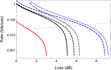
Figure 4: Composable secret key rate (bits/use) versus total loss (decibels) for the heterodyne protocol with LLO. We plot the rates against collective attacks assuming a trusted-loss and trusted-noise receiver (black dotted), a trusted-noise receiver (black dashed), and an untrusted receiver (solid black). We also show the performance achievable with the untrusted receiver in the presence of general attacks (red). The gray line is the total excess noise $\xi_{\text{tot}}$ in shot noise units. Finally, the blue lines refer to line-of-sight security (discussed in Sec. III.1) for trusted-loss and trusted-noise receiver (blue dotted), and trusted-noise receiver (blue dashed). Physical and protocol parameters are chosen as in Tables 1 and 2.

III Security of near-range free-space quantum communications

Let us now discuss the specific setting of free-space quantum communications which generally requires some elaborations of the formulas above in order to account for the additional physical processes occurring in this scenario. In the following we discuss one potential extra simplification and realistic assumption for security, and then we treat the issues related to near-range wireless communications at various frequencies and with different types of receivers (fixed or mobile).

III.1 Line-of-sight security

The line-of-sight (LoS) security is a strong but yet realistic assumption for free-space quantum communications in the near range (say within $100$ meters or so). The idea is that transmitter and receiver can “see” each other, so it is unlikely that Eve is able to tamper with the middle channel. A realistic attack is here to collect photons which are lost in the environment; in other words it is a passive attack which can be interpreted as the action of a pure-loss channel, i.e., a beam-splitter with no injection of thermal photons (which are the active entangled probes employed in the usual entangling-cloner attack).

Within the LoS assumption, there are additional degrees of reality for Eve’s attack. The most realistic scenario is Eve using a relatively-small device which only collects a fraction of the photons that are leaked into the environment. The worst-case picture which can be used as a bound for the key is to assume Eve collecting all the leaked photons. In this case, the performance will strictly depend on how much the receiver is able to intercept of the incoming beam which is in turn related to the geometric features of the beam itself (collimated, focused, or spherical beam). In any case, any thermal noise which is present in the environment is considered to be trusted.

In the studies below, we consider both LoS security (Eve passive on the channel) and standard security (Eve active on the channel). Under LoS security, thermal noise is considered to be trusted, which means that the relevant models for the detector are those with trusted noise [Eve (2)] and trusted noise and loss [Eve (1)]. The attack can be represented as in Fig. 1 but where Eve does not control environmental modes, represented by mode $e$ for Eve (1) and modes $e$,$v$ for Eve (2). With the trusted-noise detector, we also allow Eve to collect leakage from Bob’s setup; with the trusted-noise-and-loss detector, this additional side-channel is excluded. Depending on the cases, we adopt one assumption or the other. See Table 3 for a summary of the security types and trust levels (associated detector models). These definitions are meant to be in addition to the classification into individual, collective and coherent/general attacks.

Channel noise	Security type	Detector model
Untrusted	Standard security (Active Eve controlling the environment)	$\bullet~{}$Untrusted [Eve (3)] $\bullet$ Noise-trusted [Eve (2)] $\bullet~{}$Noise-loss-trusted [Eve (1)]
Trusted	LoS security (Passive Eve. No control of the environment)	$\bullet~{}$Noise-trusted [Eve (2)] $\bullet~{}$Noise-loss-trusted [Eve (1)]

Table 3: Security types and trust levels (detector models). The security assumptions become stronger from top to bottom.

The secret key rates under LoS security are derived by excluding Eve from the control of the environmental noise. This means that her CM is reduced from the form in Eq. (19) to just the block $\phi\mathbf{I}$. Thus, we have to consider the simpler joint CM for Bob and Eve

$$\mathbf{V}_{BE}=\left(\begin{array}[c]{cc}b\mathbf{I}&\theta\mathbf{I}\\ \theta\mathbf{I}&\phi\mathbf{I}\end{array}\right),$$ (71)

leading to the conditional CMs

$$\mathbf{V}_{E|B}^{\text{hom}}=\left(\begin{array}[c]{cc}\phi-\frac{\theta^{2}}{b}&0\\ 0&\phi\end{array}\right),~{}\mathbf{V}_{E|B}^{\text{het}}=\left(\phi-\frac{\theta^{2}}{b+1}\right)\mathbf{I}.$$ (72)

Therefore, Eve’s Holevo bound to be used in the key rates is simply given by

$$\chi_{\text{LoS}}^{\text{hom}}(E :y)=H(\phi)-H\left[\sqrt{\phi(\phi-\theta^{2}/b)}\right],$$ (73)

$$\chi_{\text{LoS}}^{\text{het}}(E :y)=H(\phi)-H\left(\phi-\frac{\theta^{2}}{b+1}\right),$$ (74)

where the explicit expressions for $\theta$ and $\phi$ depend on the detector noise model, while $b$ is given in Eq. (21).

Using these expressions, we may then write the asymptotic key rate with LoS security for the two detector models ($k=1,2$). Recalling that the mutual information is expressed as in Eq. (7), the LoS key rate is given by

$$R_{\text{asy,LoS}}^{(k)}(\tau,\bar{n},\bar{n}_{B})=\beta I(x:y)_{\tau,\bar{n}}-\chi_{\text{LoS}}(E:y)_{\tau,\bar{n},\bar{n}_{B}},$$ (75)

taking specific expressions for the homodyne protocol [$R_{\text{asy,LoS,hom}}^{(k)}$] and the heterodyne protocol [$R_{\text{asy,LoS,het}}^{(k)}$]. After parameter estimation, the modified key rate will be expressed in terms of the worst-case estimators as $R_{\text{pe,LoS}}^{(k)}=R_{\text{asy,LoS}}^{(k)}(\tau^{\prime},\bar{n}^{\prime},\bar{n}_{B}^{\prime})$. Finally, the composable finite-size LoS key rate takes the expression in Eq. (55) proviso we make the replacement $R_{\text{pe}}^{(k)}\longrightarrow R_{\text{pe,LoS}}^{(k)}$. Improvement in performance is shown in Fig. 4.

III.2 Optical wireless with fixed devices

Let us consider a free-space optical link between transmitter and receiver. Assume that this is mediated by a Gaussian TEM₀₀ beam with initial spot-size $w_{0}$ and phase-front radius of curvature $R_{0}$ Goodman ; Siegman ; svelto . This beam has a single well-defined polarization (scalar approximation) and carrier frequency $\nu=c/\lambda$, with $\lambda$ being the wavelength and $c$ the speed of light (so angular frequency is $\omega=2\pi c/\lambda$, and wavenumber is $k=\omega/c=2\pi/\lambda$). The pulse duration $\Delta t$ and frequency bandwidth $\Delta\nu$ satisfy the time-bandwidth product for Gaussian pulses, i.e., $\Delta t\Delta\nu\gtrsim 0.44$. In particular, we may assume $\Delta t\Delta\nu\simeq 1$. Under the paraxial wave approximation, we assume free-space propagation along the $z$ direction with no limiting apertures in the transverse plane, neglecting diffraction effects at the transmitter (e.g., by assuming a suitable aperture for the transmitter with radius $\geq 2w_{0}$ Siegman ).

By introducing the Rayleigh range

$$z_{R}:=\frac{\pi w_{0}^{2}}{\lambda},$$ (76)

which identifies near- and far-field, we may write the following expression for the diffraction-limited spot size of the beam at generic distance $z$ Siegman ; svelto

$$w_{z}^{2}=w_{0}^{2}\left[\left(1-\frac{z}{R_{0}}\right)^{2}+\left(\frac{z}{z_{R}}\right)^{2}\right].$$ (77)

In particular, for a collimated beam ($R_{0}=\infty$), we get

$$w_{z}^{2}=w_{0}^{2}[1+(z/z_{R})^{2}],$$ (78)

while for a focused beam ($R_{0}=z$), we have

$$w_{z}^{2}=w_{0}^{2}(z/z_{R})^{2}=\left(\frac{\lambda z}{\pi w_{0}}\right)^{2}.$$ (79)

We see that, in the far field $z\gg z_{R}$, the expressions in Eqs. (78) and (79) tend to coincide.

Consider then a receiver with a sharped-edged circular aperture with radius $a_{R}$. The total power impinging on this aperture is given by

$$P(z,a_{R})=\frac{\pi w_{0}^{2}}{2}\eta_{\text{d}},~{}\eta_{\text{d}}:=1-e^{-2a_{R}^{2}/w_{z}^{2}},$$ (80)

where parameter $\eta_{\text{d}}$ is the non-unit transmissivity of the channel due to the free-space diffraction and the finite size of the receiver. Note that, for far field and a receiver’s size comparable with the transmitter’s (so $a_{R}\simeq w_{0}$), we have $w_{z}\gg a_{R}$ and therefore the approximation

$$\eta_{\text{d}}\simeq\eta_{\text{d}}^{\text{far}}:=2a_{R}^{2}/w_{z}^{2}\ll 1.$$ (81)

For a collimated or focused beam, this becomes

$$\eta_{\text{d}}^{\text{far}}\simeq 2\left(\frac{\pi w_{0}a_{R}}{\lambda z}\right)^{2}.$$ (82)

The overall transmissivity of the system can be written as $\tau=\eta_{\text{ch}}\eta_{\text{eff}}$, where $\eta_{\text{ch}}=\eta_{\text{d}}\eta_{\text{atm}}$ is the total transmissivity of the external channel which generally includes the effect of atmospheric extinction $\eta_{\text{atm}}$. Since the latter effect is negligible at short distances ($\eta_{\text{atm}}\simeq 1$), we may just write $\eta_{\text{ch}}\simeq\eta_{\text{d}}$. By contrast, the other term $\eta_{\text{eff}}$ is the total quantum efficiency of the receiver and its contribution is typically non-negligible, e.g., $\eta_{\text{eff}}\simeq 0.7$. Because the devices are assumed to be fixed, there is no fading, meaning that the total transmissivity can be assumed to be constant and equal to $\tau$.

The quantum communication scenario can be described as in Fig. 1, where $\eta_{\text{ch}}$ is essentially given by free-space diffraction and the thermal background $\bar{n}_{B}$ needs to be carefully evaluated from the sky brightness (see below). Then, we can certainly assume standard security with the trust levels $k=0,1,2$ according to which Eve’s interaction is described by different effective beam-splitters with different amounts of input thermal noise $\bar{n}_{e}^{(k)}$ (see Sec. II.3). Similarly, we may investigate LoS security where thermal noise is assumed to be trusted.

Sky brightness $B_{\lambda}^{\text{sky}}$ is measured in W m^-2 nm^-1 sr^-1 and its value typically varies from $\simeq 1.5\times 10^{-6}$ (clear night) to $\simeq 1.5\times 10^{-1}$ (cloudy day) Miao ; BrussSAT , if one assumes that the receiver field of view is shielded from direct exposition to bright sources (e.g., the sun). Let us assume a receiver with aperture $a_{R}$ and angular field of view $\Omega_{\text{fov}}$ (in steradians). Assume the receiver has a detector with bandwidth $W$ and spectral filter $\Delta\lambda$. Then, the mean number of background thermal photons per mode collected by the receiver is equal to

$$\bar{n}_{B}=\frac{\pi\lambda\Gamma_{R}}{hc}B_{\lambda}^{\text{sky}},~{}\Gamma_{R}:=\Delta\lambda W^{-1}\Omega_{\text{fov}}a_{R}^{2}.$$ (83)

In this formula, we can estimate $\Omega_{\text{fov}}^{1/2}\simeq 2\arctan[l_{\text{D}}/(2f_{\text{D}})]$ from the linear size of the sensor of the detector $l_{\text{D}}$ and the focal length $f_{\text{D}}$ of the receiver. For $l_{\text{D}}=2~{}$mm and $f_{\text{D}}=20~{}$cm, we find $\Omega_{\text{fov}}\simeq 10^{-4}~{}$sr. Note that the latter value of the field of view is relatively-large compared with typical values considered in long-range setting, including satellite communications (where $\Omega_{\text{fov}}\simeq 10^{-10}~{}$sr).

The effective value of the spectral filter $\Delta\lambda$ can be very narrow in setups that are based on homodyne/heterodyne detection. The reason is because the required mode-matching of the signal with the LO pulse provides a natural interferometric process which effectively reduces the filter potentially down to the time-product bandwidth. For instance, for an LO pulse of $\Delta t_{\text{LO}}=10~{}$ns, we may assume a bandwidth $\Delta\nu=50~{}$MHz which is $\geq 0.44/\Delta t_{\text{LO}}$. Thus, interferometry at the homodyne setup imposes an effective filter of $\Delta\lambda=\lambda^{2}\Delta\nu/c\simeq 0.1~{}$pm around $\lambda=800~{}$nm.

Finally, if we take the detector bandwidth $W=100~{}$MHz and we assume a small area for the receiver’s aperture, i.e., $a_{R}=1~{}$cm (so as to be compatible with the typical sizes of near-range devices), then we compute $\bar{n}_{B}\simeq 0.019$ photons per mode during a cloudy day. This is a non-trivial amount of noise that leads to a clear discrepancy between the performance in standard security (where channel’s noise is considered to be untrusted) and LoS security (where this noise is assumed to be trusted). Let us also remark here that LoS security is a realistic assumption for receivers with a small field of view, so the noise collected from free space is limited and unlikely to come from an active Eve hidden in the environment.

For our numerical study we consider the physical parameters listed in Table 4; these are compatible with indoor and near-range optical wireless communications with small devices (e.g., laptops). This means that, for the transmitter, we consider limited power (e.g., $10~{}$mW), and a small spot size ($w_{0}=1~{}$mm). Similarly, for the receiver, we consider a limited aperture ($a_{R}=1~{}$cm), non-unit quantum efficiency ($\eta_{\text{eff}}=0.7$), and a realistic field of view $\Omega_{\text{fov}}\simeq 10^{-4}~{}$sr as discussed above.

Physical parameter	Symbol	Value
Altitude	$h$	$30$ m
Beam curvature	$R_{0}$	$\infty$ (collimated)
Wavelength	$\lambda$	$800~{}$nm
Beam spot size	$w_{0}$	$1~{}$mm
Receiver aperture	$a_{R}$	$1$ cm
Receiver field of view	$\Omega_{\text{fov}}$	$10^{-4}~{}$sr
Homodyne filter	$\Delta\lambda$	$0.1~{}\text{pm}$
Detector shot-noise	$\nu_{\text{det}}$	$2~{}\text{(het)}$
Detector efficiency	$\eta_{\text{eff}}$	$0.7$ ($1.55~{}$dB)
Detector bandwidth	$W$	$100~{}$MHz
Noise equivalent power	NEP	$6~{}$pW/$\sqrt{\text{Hz}}$
Linewidth	$l_{\text{W}}$	$1.6$ KHz
LO power	$P_{\text{LO}}$	$10~{}$mW
Clock	$C$	$5~{}$MHz
Pulse duration	$\Delta t,\Delta t_{\text{LO}}$	$10~{}$ns
Setup noise with LLO	$\bar{n}_{\text{ex}}$	Eq. (17)
Channel noise	$\bar{n}_{B}$	$0.019$ [Eq. (83)]
Total thermal noise	$\bar{n}$	Eq. (3)
Atmospheric extinction	$\eta_{\text{atm}}$	$\simeq 1$ (negligible)

Table 4: Physical parameters for optical wireless

Assuming the physical parameters in Table 4 and the protocols parameters in Table 2, we show the various achievable performances of the free-space diffraction-limited heterodyne protocol with LLO in Fig. 5. As we can see from the figure, we have drastically different rates depending on the type of security and trust level. It is clear that the highest rates (and distances) are obtained with LoS security (blue lines in the figure). With standard security, the range is restricted to about $50$ meters (black lines in the figure) and about $30$ meters in the worst-case scenario of an untrusted detector and general attacks (red line in the figure). The possibility to enforce weaker security assumptions leads to non-trivial advantages in terms of rate and distance.

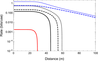
Figure 5: Optical-wireless QKD with fixed devices. We plot the composable secret key rate (bits/use) versus free-space distance (meters) for the heterodyne protocol with LLO. In particular, we show the rates against collective attacks assuming a trusted-loss-and-noise receiver (black dotted), a trusted-noise receiver (black dashed), and an untrusted receiver (solid black). We also show the performance achievable with the untrusted receiver versus general attacks (red). The blue lines refer to line-of-sight security (discussed in Sec. III.1) for trusted-loss-and-noise receiver (blue dotted), and trusted-noise receiver (blue dashed). Physical parameters are chosen as in Table 4, while protocol parameters are in Table 2.

Also note the stability of the rates at short distances ($<30~{}$m) where their values remain approximately constant. This is due to the fact that, for the specific regime of parameters considered, the beam broadening induced by free-space diffraction within that range [see Eq. (78) with $w_{0}=1~{}$mm and $z<30$ m] is still limited with respect to the radius of the receiver’s aperture ($a_{R}=1~{}$cm). Thus, the transmissivity $\eta_{\text{d}}$ in Eq. (80) remains sufficiently close to $1$, before starting to decay after about $30$ m.

III.3 Optical wireless with mobile devices

III.3.1 Pointing and tracking error

In the presence of free-space optical connections with portable devices, one can use a suitable tracking mechanism so the transmitter (such as a fixed router/hot spot) points at the mobile receiver in real time with some small pointing error. In general, the receiver too may have a mechanism of adaptive optics aimed at maintaining the beam alignment by rotating the field of view in direction of the transmitter. We therefore need to introduce a pointing error at the transmitter $\tilde{\sigma}_{\text{P}}$ which introduces a Gaussian wandering of the beam centroid over the receiver’s aperture with variance $\sigma_{\text{P}}^{2}\simeq(\tilde{\sigma}_{\text{P}}z)^{2}$ for distance $z$. We assume an accessible value $\tilde{\sigma}_{\text{P}}\simeq 1.745\times 10^{-3}$ radiant, which is about $1/10$ of a degree (this is orders-of-magnitude worse than the performance achievable in satellite-based pointing and tracking).

Let us call $r$ the instantaneous deflection of the beam centroid from the center of the receiver’s aperture. The wandering can be described by the Weibull distribution

$$P_{\text{WB}}(r)=\frac{r}{\sigma_{\text{P}}^{2}}\exp\left(-\frac{r^{2}}{2\sigma_{\text{P}}^{2}}\right).$$ (84)

For each value of the deflection $r$, there is an associated instantaneous transmissivity $\tau=\tau(r)$, which can be computed as follows

$$\tau(r)=e^{-\frac{4r^{2}}{w_{z}^{2}}}Q_{0}\left(\frac{2r^{2}}{w_{z}^{2}},\frac{4ra_{R}}{w_{z}^{2}}\right),$$ (85)

where $Q_{0}(x,y)$ is an incomplete Weber integral Agrest .

Alternatively, we may use the approximation

$$\tau(r)\simeq\eta\exp\left[-\left(\frac{r}{r_{0}}\right)^{\gamma}\right],$$ (86)

where

$$\eta:=\tau(0)=\eta_{\text{ch}}(z)\eta_{\text{eff}}\simeq\eta_{\text{d}}(z)\eta_{\text{eff}}$$ (87)

is the maximum transmissivity at distance $z$ (corresponding to a beam that is perfectly-aligned), while$\ \gamma$ and $r_{0}$ are the following shape and scale (positive) parameters

$$\gamma =\frac{4\eta_{\text{d}}^{\text{far}}\Lambda_{1}(\eta_{\text{d}}^{\text{far}})}{1-\Lambda_{0}(\eta_{\text{d}}^{\text{far}})}\left[\ln\frac{2\eta_{\text{d}}}{1-\Lambda_{0}(\eta_{\text{d}}^{\text{far}})}\right]^{-1},$$ (88)

$$r_{0} =a_{R}\left[\ln\frac{2\eta_{\text{d}}}{1-\Lambda_{0}(\eta_{\text{d}}^{\text{far}})}\right]^{-\frac{1}{\gamma}},$$ (89)

where $\Lambda_{n}(x):=e^{-2x}I_{n}\left(2x\right)$ and $I_{n}$ is a modified Bessel function of the first kind with order $n$ (Vasy12, , Eq. (D2)).

By suitably combining Eqs. (84) and (86), one can derive the fading statistics, i.e., the probability distribution $P_{\text{fad}}$ associated with the instantaneous transmissivity $\tau$, which is given by

$$P_{\text{fad}}(\tau)=\frac{r_{0}^{2}}{\gamma\sigma_{\text{P}}^{2}\tau}\left(\ln\frac{\eta}{\tau}\right)^{\frac{2}{\gamma}-1}\exp\left[-\frac{r_{0}^{2}}{2\sigma_{\text{P}}^{2}}\left(\ln\frac{\eta}{\tau}\right)^{\frac{2}{\gamma}}\right].$$ (90)

III.3.2 Maximum wireless range

Besides the beam wandering (and associated fading) due to pointing and tracking error, there is also the further issue that a mobile receiver generally has a variable distance from the transmitter, so the transmissivity of the free-space link has an additional degree of variability. The latter effect has a very slow dynamics with respect to typical clocks, meaning that a block of reasonable size is distributed while the position of the receiver is substantially unchanged. For example, for a detector bandwidth $W=100~{}$MHz, we may use a clock of $C=W/3\simeq 33~{}$MHz. In this case, a block of $10^{7}$ points will be distributed in $1/3$ of a second. For an indoor network, assuming an average walking speed of $\simeq 1.5$ m/s, this corresponds to a $\simeq 50$ cm free-space displacement of the receiver. In the worst-case scenario where this displacement increases the distance from the transmitter, we may assume that the distribution of the whole block occurs at the maximum distance.

In general, we may compute a lower bound by assuming that the entire quantum communication (i.e., the communication of all the blocks) occurs with the mobile device at the maximum distance from the transmitter. In other words, we can fix a maximum range $z_{\text{max}}$ for the local network and assume this value as worst-case scenario. Since the parties control the parameters of the channel and know the instantaneous distance, they could process their data in a way that it appears to be completely distributed at $z_{\text{max}}$ (data distributed at $z<z_{\text{max}}$ can be attenuated and suitably thermalized in post processing).

To be more precise the lower bound should be computed by minimizing the transmissivity and maximizing the thermal noise over the distance $z\leq z_{\text{max}}$, so that data is processed via a more lossy and noisy channel. While the minimization of the transmissivity occurs at $z=z_{\text{max}}$, the maximization of the thermal noise may occur at different values of $z$, depending on the type of LO. In particular, this value is $z=z_{\text{max}}$ for the TLO and $z=0$ for the LLO. The issue is therefore resolved for the LLO if we keep the mobile device at $z=z_{\text{max}}$ while bounding the LLO noise with the value for $z=0$.

Such an approach is not optimal but robust and applicable to outdoor wireless networks with faster-moving devices (with a speed limited by the ratio between $z_{\text{max}}$ and the total communication time). It is worth mentioning that, a better but more complicated strategy relies on slicing the trajectory of the moving device into sectors, with each sector being associated with the communication of a single block and the final rate being given by the average rate over the sectors. This is particularly useful in satellite quantum communications where a trajectory is well defined (for instance, see the technique of orbital slicing in Ref. SATpaper ). However, for stochastic trajectories on the ground, the analytical treatment is not immediate.

III.3.3 Pilot modes and de-fading

Besides the use of bright pointing/tracking modes and bright LLO-reference modes, it is also important to use relatively-bright pilot modes that are specifically employed for the real-time estimation of the instantaneous transmissivity $\tau$, whose fluctuation is generally due to both pointing error and distance variability (for mobile devices). These $m_{\text{PL}}$ pilots are randomly interleaved with $N_{\text{S}}:=N-m_{\text{PL}}$ signal modes, where $N$ are the total pulses. The pilots allow the parties to: (i) identify an overall interval for the transmissivity $\Delta=[\tau_{\min},\tau_{\max}]$ in which $N_{\text{S}}p_{\Delta}$ signals are post-selected with probability $p_{\Delta}$; (ii) introduce a lattice in $\Delta$ with step $\delta\tau$, so that each signal is associated with a corresponding narrow bin of transmissivities $\Delta_{k}:=[\tau_{k},\tau_{k+1}]$, with $\tau_{k}:=\tau_{\min}+(k-1)\delta\tau$ for $k=1,\ldots,M$ and $M=(\tau_{\max}-\tau_{\min})/\delta\tau$ NotePilots .

Each bin $\Delta_{k}$ is selected with probability $p_{k}$ and, therefore, populated by $N_{\text{S}}p_{k}$ signals. There are corresponding $\nu_{\text{det}}N_{\text{S}}p_{k}$ pairs of points $\{x_{i},y_{i}\}$ satisfying the input-output relation of Eq. (4), which here reads

$$y^{(k)}\simeq\sqrt{\tau_{k}}x+z^{(k)},$$ (91)

where $z^{(k)}$ is a Gaussian noise variable with variance

$$\sigma_{k}^{2}=2\bar{n}_{k}+\nu_{\text{det}},~{}\bar{n}_{k}:=\eta_{\text{eff}}\bar{n}_{B}+\bar{n}_{\text{ex}}(\tau_{k}).$$ (92)

Bob can map these points into the first bin $\Delta_{1}$ of the interval via the de-fading map

$$y^{(k)}\rightarrow\tilde{y}^{(k)}=\sqrt{\frac{\tau_{\text{min}}}{\tau_{k}}}y^{(k)}+\sqrt{1-\frac{\tau_{\text{min}}}{\tau_{k}}}\xi_{\text{add}},$$ (93)

where $\xi_{\text{add}}$ is Gaussian noise with variance $\nu_{\text{det}}$.

By repeating this procedure for all the bins, Bob create the new variable

$$\tilde{y}=\sqrt{\tau_{\text{min}}}x+\tilde{z},$$ (94)

where $\tilde{z}$ is non-Gaussian noise with variance

$$\sigma_{\tilde{z}}^{2}=2\bar{n}_{\ast}+\nu_{\text{det}},~{}\bar{n}_{\ast}:=\frac{\tau_{\text{min}}}{p_{\Delta}}\sum_{k}\frac{p_{k}}{\tau_{k}}\bar{n}_{k}.$$ (95)

This new variable is now associated with a single (worst-case) transmissivity $\tau_{\text{min}}$, thus effectively removing the fading process from the distributed data, i.e., from their $\nu_{\text{det}}N_{\text{S}}p_{\Delta}$ pairs of correlated points.

Exploiting the optimality of Gaussian attacks, the parties assume that $\tilde{z}$ is Gaussian (overestimating Eve’s performance). In this way, the final input-output relation in Eq. (94) reduces to considering a simpler thermal-loss Gaussian channel with transmissivity $\tau_{\text{min}}$ and thermal number $\bar{n}_{\ast}$. See Ref. FSpaper for more details.

For a receiver at some fixed distance $z$ and only subject to pointing error, we can assume $\tau_{\max}=\eta$ [cf. Eq. (87)] and $\tau_{\text{min}}=f_{\text{th}}\eta$ for some threshold factor $f_{\text{th}}<1$. Then, the probabilities $p_{\Delta}=p(\tau_{\text{min}},\tau_{\text{max}})$ and $p_{k}=p(\tau_{k},\tau_{k+1})$ are computed from the formula

$$p(\tau_{1},\tau_{2}):=\int_{\tau_{1}}^{\tau_{2}}d\tau~{}P_{\text{fad}}(\tau),$$ (96)

where $P_{\text{fad}}(\tau)$ is given in Eq. (90).

In general, for a mobile receiver at variable distance $z$, Alice and Bob compute the post-selection interval $\Delta$ and the lattice $\{\Delta_{k}\}$ directly from data, together with the corresponding values of $p_{\Delta}$ and $p_{k}$. As mentioned in the previous subsection, the performance in this general scenario can be lower-bounded by the extreme case where the receiver is assumed to be fixed at the maximum distance $z_{\text{max}}$ from the transmitter (while maximizing thermal noise over $z$, whose maximum is at $z_{\text{max}}$ for a TLO and at $z=0$ for an LLO). In this worst-case scenario, we may exploit the formula in Eq. (96) for the fading probability (suitably computed at $z_{\text{max}}$) and derive an analytical lower bound for the secret key rate.

III.3.4 Estimators and key rate

Let us assume the worst-case scenario of a receiver at the maximum range $z_{\text{max}}$ from the transmitter, so the maximum transmissivity is $\tau_{\max}=\eta(z_{\text{max}})$ and the minimum transmissivity is $\tau_{\text{min}}=f_{\text{th}}\eta(z_{\text{max}})$ for some threshold value $f_{\text{th}}$. These border values define a post-selection interval $\Delta$ which is sliced into a lattice of $M$ narrow bins $\{\Delta_{k}\}$. The instantaneous transmissivity $\tau$ will fluctuate according to the distribution in Eq. (90) with associated pointing error $\sigma_{z_{\text{max}}}^{2}\simeq(\sigma_{\text{P}}z_{\text{max}})^{2}$ for an empirical value $\sigma_{\text{P}}$ at the transmitter (e.g., $1/10$ of a degree). As a result of the fluctuation, a value of the transmissivity $\tau$ is post-selected with probability $p_{\Delta}$ and populates bin $\Delta_{k}$ with probability $p_{k}$, according to the integral in Eq. (96).

For the worst-case scenario, let us also assume that the thermal noise is maximized over $z\leq z_{\text{max}}$ (and the fading process). Thus, for any bin $\Delta_{k}$, we consider the following bound on the associated thermal noise

$$\bar{n}_{k}\leq\bar{n}_{\text{wc}}=\eta_{\text{eff}}\bar{n}_{B}+\bar{n}_{\text{ex,wc}},$$ (97)

where the maximum setup noise $\bar{n}_{\text{ex,wc}}$ depends on the type of LO and is given by

$$\bar{n}_{\text{ex,wc}}^{\text{TLO}}\simeq\Theta_{\text{el}}/\tau_{\text{min}},~{}\bar{n}_{\text{ex,wc}}^{\text{LLO}}\simeq\Theta_{\text{el}}+\pi\sigma_{x}^{2}C^{-1}l_{\text{W}}.$$ (98)

Note that the first expression in Eq. (98) above is computed on $\tau_{\text{min}}=\tau_{\text{min}}(z_{\text{max}})$ while the second one is computed for $\tau=1$ (maximum value at $z=0$). By replacing Eq. (97) in Eq. (95), we get the bound

$$\bar{n}_{\ast}\leq\bar{n}_{\text{wc}}.$$ (99)

As already explained, the construction of the lattice is possible thanks to the random pilots. In total, during the quantum communication, the parties exchange $N$ quantum pulses, whose $m_{\text{PL}}$ are pilots and $N_{\text{S}}=N-m_{\text{PL}}$ are signals. Using the pilots, the parties post-select a fraction $N_{\text{S}}p_{\Delta}$ of the signals, with a smaller fraction $N_{\text{S}}p_{k}$ allocated to the generic bin $\Delta_{k}$. After de-fading, the parties are connected by an effective thermal-loss channel with transmissivity $\tau_{\text{min}}=\tau_{\text{min}}(z_{\text{max}})$ and thermal number $\bar{n}_{\text{wc}}$.

The parties sacrifice a portion $mp_{\Delta}$ of the post-selected signals $N_{\text{S}}p_{\Delta}$ for parameter estimation (PE), so $np_{\Delta}$ signals are left for key generation, where $n=N_{\text{S}}-m$ (this value is further reduced for security extended to general coherent attacks). Overall the parties use $m_{\Delta}:=\nu_{\text{det}}mp_{\Delta}$ pairs of data points for PE following the procedure described in Sec. II.5 with effective transmissivity $\tau_{\text{min}}=\tau_{\text{min}}(z_{\text{max}})$ and $\sigma_{\text{wc}}^{2}=2\bar{n}_{\text{wc}}+\nu_{\text{det}}$. This leads to the following bounds for the worst-case estimators FSpaper

$$\tau_{\text{LB}} =\tau_{\text{min}}-2w\sqrt{\frac{2\tau_{\text{min}}^{2}+\tau_{\text{min}}\sigma_{\text{wc}}^{2}/\sigma_{x}^{2}}{m_{\Delta}}},$$ (100)

$$\bar{n}_{\text{UB}} =\bar{n}_{\text{wc}}+w\frac{\sigma_{\text{wc}}^{2}}{\sqrt{2m_{\Delta}}},$$ (101)

where $\sigma_{x}^{2}$ is the input modulation and $w$ is the confidence parameter [cf. Eqs. (46) and (47)].

As we can see from the two estimators above, the relevant information is the minimum transmissivity $\tau_{\text{min}}$ of the post-selection interval, the maximum thermal noise $\bar{n}_{\text{wc}}$ over the range (and fading process), and the number of post-selected points $m_{\Delta}$. The formulas hold for a generic fading statistics, i.e., not necessarily given by Eq. (96), as long as we can evaluate $m_{\Delta}$. Also note that, assuming Eq. (96) and fixing a threshold transmissivity $\tau_{\text{min}}$, the value of $m_{\Delta}$ decreases by increasing $z$. In other words, the fact that a worst-case device at the maximum range provides a lower bound for a mobile device is also due to the decreased statistics for PE.

In order to compute the key rates for the trusted models, we also need to bound the worst-case estimator of the background thermal noise $\bar{n}_{B}$. This is possible by writing

$$\bar{n}_{B}^{\text{UB}}=\frac{\bar{n}_{\text{UB}}-\bar{n}_{\text{ex,bc}}}{\eta_{\text{eff}}},$$ (102)

where the best-case value $\bar{n}_{\text{ex,bc}}$ needs to be optimized over the entire range $z\leq z_{\max}$ and the fading process. We therefore extend Eqs. (48) and (49) to the following expressions

$$\bar{n}_{\text{ex,bc}}^{\text{TLO}}:=\Theta_{\text{el}},~{}\bar{n}_{\text{ex,bc}}^{\text{LLO}}:=\Theta_{\text{el}}+\Theta_{\text{ph}}\tau_{\text{min}}.$$ (103)

We now have all the elements to write the composable finite-size key rate, which extends Eq. (55) of Sec. II.6 to the following expression

$$R\geq\frac{np_{\Delta}p_{\text{ec}}}{N}\left(R_{\text{pe}}^{(k)}-\frac{\Delta_{\text{aep}}}{\sqrt{np_{\Delta}}}+\frac{\Theta}{np_{\Delta}}\right),$$ (104)

where $n=N-(m+m_{\text{PL}})$ and $R_{\text{pe}}^{(k)}$ depends on the receiver model ($k=1,2,3$). The latter takes the following expressions in terms of the new estimators

$$R_{\text{pe}}^{(1,2)} =R_{\text{asy}}^{(1,2)}(\tau_{\text{LB}},\bar{n}_{\text{UB}},\bar{n}_{B}^{\text{UB}}),$$ (105)

$$R_{\text{pe}}^{(3)} =R_{\text{asy}}^{(3)}(\tau_{\text{LB}},\bar{n}_{\text{UB}}).$$ (106)

Alternatively, we may write Eq. (104) assuming LoS security, which means to replace $R_{\text{pe}}^{(k)}$ with the key rate

$$R_{\text{pe,LoS}}^{(k)}=R_{\text{asy,LoS}}^{(k)}(\tau_{\text{LB}},\bar{n}_{\text{UB}},\bar{n}_{B}^{\text{UB}}).$$ (107)

The composable key rate in Eq. (104) is $\varepsilon$-secure against collective Gaussian attacks [cf Eq. (59)].

For the heterodyne protocol, we extend the composable key rate of Eq. (70) to the following expression

$$R_{\text{gen}}^{\text{het}}\geq\frac{np_{\Delta}p_{\text{ec}}}{N}\left(R_{\text{pe,het}}^{(k)}-\frac{\Delta_{\text{aep}}}{\sqrt{np_{\Delta}}}+\frac{\Theta-\Phi_{np_{\Delta}}}{np_{\Delta}}\right),$$ (108)

where $n$ must account for the $m_{\text{PL}}$ pilots besides the $m_{\mathrm{et}}$ energy tests, i.e.,

$$n=N-(m+m_{\text{PL}}+m_{\text{et}})=\frac{N-(m+m_{\text{PL}})}{1+f_{\mathrm{et}}},$$ (109)

and $R_{\text{pe,het}}^{(k)}$ is given by Eqs. (105) and (106) for the case of the heterodyne protocol. This rate has epsilon security $\varepsilon^{\prime}=K_{np_{\Delta}}^{4}\varepsilon/50$ against general attacks, with $\varepsilon$ being the initial security versus collective attacks (see Sec. II.6).

We perform a numerical investigation assuming the heterodyne protocol with LLO. This is now implemented in a post-selection fashion in a way to remove the (non-Gaussian) effect of fading from the distributed data (see above). We consider the protocol parameters in Table 2 but where we include the pilots $m_{\text{PL}}=0.05\times N$, so the key generation signals are reduced to $n\simeq 7.08\times 10^{6}$, and a threshold parameter $f_{\text{th}}=0.8$ for post-selection. We then assume the physical parameters in Table 4, but taking a higher clock value $C=33~{}$MHz and also including the transmitter’s pointing error $\tilde{\sigma}_{\text{P}}$, equal to $1/10$ of degree. In this regime of parameters, we study the composable key rates that are achievable under the various security and trust assumptions, considering a mobile device which can move up to a maximum distance $z_{\max}$ from the transmitter (range of the wireless network).

The rates are plotted in Fig. 6. Note that the values in the range of $10^{-2}-1$ bit/use correspond to high rates in the range of $0.33-33~{}$Mbits/sec at the considered clock. This means that quantum-encrypted wireless communication at about $1~{}$Mbit/sec are possible within distances of a few meters. Another important consideration is that these rates are actually lower bounds, since they are computed with the device at the maximum distance and bounding the noise. This is also the reason why the key rate of Eq. (108) does not appear for this specific choice of parameters.

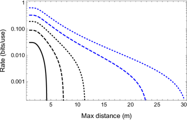
Figure 6: Optical-wireless QKD with mobile devices. We plot the composable secret key rate (bits/use) versus the maximum free-space distance $z_{\max}$ of the receiver-device from the transmitter (meters). This is for a pilot-guided post-selected heterodyne protocol with an LLO. We show the rates against collective attacks assuming a trusted-loss-and-noise receiver (black dotted), a trusted-noise receiver (black dashed), and an untrusted receiver (solid black). The blue lines refer to line-of-sight security for trusted-loss-and-noise receiver (blue dotted), and trusted-noise receiver (blue dashed). Physical parameters are chosen as discussed in the main text.

III.4 Short-range microwave wireless

Let us consider wireless quantum communications at the microwave frequencies, in particular at 1 GHz. We show the potential feasibility for short-range quantum-safe WiFi (e.g., for contact-less cards) within the general setting of composable finite-size security. First of all we need to remark two important differences with respect to the optical case: presence of higher loss and higher noise.

From the point of view of increased loss, the crucial difference is the geometry of the beam. For indoor wireless applications, microwave antennas are small and, for this reason, cannot offer beam directionality. The emitted beam is either isotropic (spherical wave) or have some limited directionality, usually quantified by the gain $g$. This means that, at some distance $z$, the intensity of the beam will be confined in an area equal to $4\pi z^{2}/g$. It is clear that we have a strong suppression of the signal, since a receiver with aperture’s radius $a_{R}$ is going to collect just a fraction $\eta_{\text{ch}}\simeq\min\{ga_{R}^{2}/(4\pi z^{2}),1\}$ of the emitted photons. Here the minimum accounts for the case where the receiver is close to the antenna, so the angle of emission is subtended by the receiver’s aperture, which happens at the distance $z_{\text{best}}=\sqrt{g/\pi}a_{R}/2$. In our investigation, we assume the numerical value $g=10$.

As mentioned above another important difference with respect to the optical case is the amount of thermal background noise which affects microwaves for both signal preparation and detection refA1 ; refA2 ; refA3 ; refA4 ; refA5 ; refA6 . If we assume setups working at room temperature, this thermal noise is dominant with respect to the other sources of noise. Both the preparation noise at the microwave modulators and the electronic noise in the amplifiers of the microwave homodyne detectors are relevant Shabir ; we set them to be equal to the thermal background computed using the formula of the black-body radiation. On the other hand, phase-errors associated with the LO are negligible since the LO is slow at the microwave and can easily be reconstructed.

Let us quantify the amount of thermal noise and identify a suitable set of parameters able to mitigate the problem. For a receiver with spectral filter $\Delta\lambda$, detector bandwidth $W$, aperture $a_{R}$, and field of view $\Omega_{\text{fov}}$, we can consider the photon collection parameter $\Gamma_{R}$ in Eq. (83). Assume that signal and LO pulses are time-bandwidth limited, so that $\Delta t\Delta\nu\simeq 1$. For instance $\Delta t=10$ ns and $\Delta\nu=100~{}$MHz for a carrier frequency of $\nu=1~{}$GHz ($10\%$ bandwidth). Corresponding carrier wavelength is $\lambda=c/\nu\simeq 30~{}$cm. Using $\Delta\lambda=\Delta\nu\lambda^{2}/c$ and setting $W\simeq\Delta\nu$ (detector resolving the pulses), we may write

$$\Gamma_{R}\simeq\frac{\lambda^{2}}{c}\Omega_{\text{fov}}a_{R}^{2}.$$ (110)

For receiver aperture $a_{R}=5~{}$cm and sufficiently-narrow field of view $\Omega_{\text{fov}}^{1/2}=1~{}$degree (so $\Omega_{\text{fov}}\simeq 3\times 10^{-4}$ sr), we compute $\Gamma_{R}\simeq 2.28\times 10^{-16}$ in units of s m³ sr. Note that realizing such a narrow field of view with a small indoor receiver can be challenging in practice.

The photon collection parameter must be combined with the thermal background photons in units of photons s^-1 m^-3 sr^-1, quantified by the black-body formula

$$\bar{n}_{\text{body}}=\frac{2c}{\lambda^{4}}\left[\exp\left(\frac{hc}{\lambda k_{\text{B}}T}\right)-1\right]^{-1},$$ (111)

where $k_{\text{B}}$ is Boltzmann’s constant and $T\simeq 290~{}$K is the temperature. Therefore we get

$$\bar{n}_{\text{th}}=\Gamma_{R}\bar{n}_{\text{body}}\simeq 0.1\text{~{}photons.}$$ (112)

Note that the figure is acceptably low thanks to the filtering effect of $\Gamma_{R}$, which accounts for the spatiotemporal profile of the LO pulses, together with the other features of the receiver (aperture, field of view).

Thermal noise is affecting both preparation and detection with constant floor level. This means that $\bar{n}_{\text{th}}$ mean photons are seen by the detector no matter if signal photons are present or not. In other words, the detector experiences a constant noise variance equal to

$$\sigma_{z}^{2}=2\bar{n}_{\text{th}}+\nu_{\text{det}},$$ (113)

where $\nu_{\text{det}}$ is the usual quantum duty (which is $=1$ for homodyne and $=2$ for heterodyne).

Assume that the total transmissivity is $\tau=\eta_{\text{ch}}\eta_{\text{eff}}$, where $\eta_{\text{ch}}$ is channel’s transmissivity and $\eta_{\text{eff}}\simeq 0.8$ is receiver’s efficiency. Also assume that the transmitter (Alice), modulates thermal states with classical variance $\sigma_{x}^{2}=2\bar{n}_{T}$, where $\bar{n}_{T}$ is equivalent mean number of signal photons. Then, the total mean number of photons at the receiver’s detector is given by

$$\bar{n}_{R}=\tau\bar{n}_{T}+\bar{n}_{\text{th}}.$$ (114)

Basically, this is equivalent to Eqs. (2) and (3), by setting $\bar{n}_{B}=\bar{n}_{\text{th}}$ and $\bar{n}_{\text{ex}}=(1-\eta_{\text{eff}})\bar{n}_{\text{th}}$. As we can see, for $\tau=1$, we get $\bar{n}_{T}+\bar{n}_{\text{th}}$ meaning that the prepared states are thermal; for $\tau<1$, signal photons are lost ($\bar{n}_{T}\rightarrow\tau\bar{n}_{T}$), while the depleted thermal background photons are compensated at the receiver re-entering the detection system, so we have the constant noise level $\bar{n}_{\text{th}}$.

III.4.1 Fully-untrusted scenario

In the worst-case scenario, the noise associated with preparation, channel and detector is all untrusted. In this case, Eq. (114) corresponds to the action of a beam splitter with transmissivity $\tau$ combining a signal mode with mean photons $\bar{n}_{T}$ and an environmental mode with mean photons $\bar{n}_{e}=\bar{n}_{\text{th}}/(1-\tau)$. The idea is that Alice would attempt to create randomly-displaced coherent states, but Eve readily thermalizes them by adding malicious thermal photons. These photons add up to those later introduced by the channel, so that we globally have the insertion of $\bar{n}_{e}$ mean photons as above. This leads to a collective Gaussian attack where Eve has the purification of the untrusted thermal noise associated with each stage of the communication.

Alice’s and Bob’s classical variables, $x$ and $y$, are related by Eq. (4) but where the noise variable $z$ has now variance $\sigma_{z}^{2}$ as in Eq. (113) which corresponds to Eq. (6) up to replacing $\bar{n}\rightarrow\bar{n}_{\text{th}}$. Alice and Bob’s mutual information $I(x:y)$ is therefore given by Eq. (7) computed with modulation $\sigma_{x}^{2}=2\bar{n}_{T}$ and equivalent noise

$$\chi=\frac{2\bar{n}_{\text{th}}+\nu_{\text{det}}}{\tau}=\xi_{\text{tot}}+\frac{\nu_{\text{det}}}{\tau},$$ (115)

where $\xi_{\text{tot}}:=2\bar{n}_{\text{th}}/\tau$ is the total excess noise. Numerically, we choose the modulation $\sigma_{x}^{2}=20$.

As already said, in the fully-untrusted scenario, all thermal noise coming from preparation, channel and receiver’s setup is considered to be untrusted. This is equivalent to the treatment of Sec. II.4.3, proviso we make the replacement $\bar{n}\rightarrow\bar{n}_{\text{th}}$ in Eq. (34) and then in Eqs. (21), (22) and (23). The revised parameters can then be used in the global CM in Eqs. (18) and (19).

Then, the asymptotic key rate against collective Gaussian attacks is given by $R_{\text{asy}}^{(3)}(\tau,\bar{n}_{\text{th}})$ according to Eq. (40), where we now use

$$\tau=\eta_{\text{eff}}\min\{ga_{R}^{2}/(4\pi z^{2}),1\},$$ (116)

and $\bar{n}_{\text{th}}$ as given by Eq. (112). We may then assume the reconciliation parameter $\beta=0.98$.

To account for finite-size effects, we first include parameter estimation. This means that the parties need to sacrifice $m$ of the $N$ pulses, so $n$ pulses survive for key generation. Numerically, we take $N=5\times 10^{7}$ and $m=0.1\times N$. Thus, they construct the worst-case estimators for the overall transmissivity $\tau$ and thermal noise $\bar{n}_{\text{th}}$ following Eqs. (44) and (45). These estimators can be here approximated as follows

$$\tau^{\prime} \simeq\tau-2w\sqrt{\frac{2\tau^{2}+\tau(2\bar{n}_{\text{th}}+\nu_{\text{det}})/\sigma_{x}^{2}}{\nu_{\text{det}}m}},$$ (117)

$$\bar{n}_{\text{th}}^{\prime} \simeq\bar{n}_{\text{th}}+w\frac{2\bar{n}_{\text{th}}+\nu_{\text{det}}}{\sqrt{2\nu_{\text{det}}m}},$$ (118)

where $w$ is the confidence parameter associated with $\varepsilon_{\text{pe}}$, and computed according to Eq. (46) for collective Gaussian attacks (see Sec. II.5 for more details). Assuming a tolerable error probability of $\varepsilon_{\text{pe}}=2^{-33}$, we have $w\simeq 6.34$ confidence intervals.

The composable key rate takes the form in Eq. (55) where we now use $R_{\text{pe}}^{(3)}=R_{\text{asy}}^{(3)}(\tau^{\prime},\bar{n}_{\text{th}}^{\prime})$ computed from Eqs. (117) and (118), together with the usual finite-size terms in Eqs. (57) and (58). Numerically, we can assume $p_{\text{ec}}=0.9$ for the probability of success of EC, $d=2^{5}$ for the digitalization of the continuous variables, and the value $2^{-33}$ for all the epsilon parameters, so we have epsilon security $\varepsilon\simeq 5.6\times 10^{-10}$ against collective Gaussian attacks according to Eq. (59).

To study the performance, let us consider the heterodyne protocol ($\nu_{\text{det}}=2$). Then, we assume a device stably kept at some distance $z$ from the transmitter within the emission angle of the transmitter and with an aligned field of view. For the parameters considered here, we find that a positive key rate is obtained for $z\leq 4.48$ cm, which is fully compatible for contactless card applications. In particular, for any $z\leq z_{\text{best}}\simeq 4.46$ cm we compute a key rate of $R\gtrsim 10^{-2}$ bits/use, corresponding to $\gtrsim 50$ kbit/sec with a system clock at $5$ MHz.

Note that, according to the thermal version of the PLOB bound QKDpaper , the maximum key rate cannot overcome the upper limit

$$R\leq\left\{\begin{array}[c]{l}-\log_{2}\left[(1-\tau)\tau^{\frac{\bar{n}_{\text{th}}}{1-\tau}}\right]-h\left(\frac{\bar{n}_{\text{th}}}{1-\tau}\right),~{}~{}\text{for~{}}\bar{n}_{\text{th}}\leq\tau,\\ 0,~{}~{}\text{for~{}}\bar{n}_{\text{th}}\geq\tau,\end{array}\right.$$ (119)

where $h(x):=H(2x+1)$. This means that the no rate is possible above the threshold $\bar{n}_{\text{th}}=\tau$. Using Eqs. (112) and (116) with our regime of parameters, we find that the maximum possible range is about $12.47~{}$cm, i.e., about three times the distance achievable with the considered heterodyne protocol under composable security.

III.4.2 LoS security for microwaves

Better performances can be obtained if we relax security requirements by relying on the LoS geometry. In particular, one may assume that the thermal noise is trusted, so that Eve is passively limited to eavesdrop the photons leaking from the channel and the setup. In this case, Eq. (114) corresponds to the action of a beam splitter with transmissivity $\tau$ combining a signal mode with mean photons $\bar{n}_{T}+\bar{n}_{\text{th}}$ (signal photons plus trusted preparation noise) and a genuine environmental mode with mean photons $\bar{n}_{\text{th}}$ NotaNOISE . Eve collects the fraction $1-\tau$ of photons leaked into the environment, but she does not control any noise, i.e., she does not have its purification.

Alice and Bob’s mutual information $I(x:y)$ is the same as above for the fully-untrusted case but Eve’s Holevo information $\chi_{\text{LoS}}(E:y)$ is now rather different. The latter can be computed as in Sec. III.1 and, in particular, from the CM in Eq. (71), where we insert the following parameters

$$b =2\bar{n}_{R}+1,$$ (120)

$$\theta =-\sqrt{\tau(1-\tau)}\sigma_{x}^{2},$$ (121)

$$\phi =(1-\tau)\sigma_{x}^{2}+2\bar{n}_{\text{th}}+1.$$ (122)

In this way we can compute the asymptotic key rate

$$R_{\text{asy,LoS}}(\tau,\bar{n}_{\text{th}})=\beta I(x:y)-\chi_{\text{LoS}}(E:y).$$ (123)

The incorporation of finite-size effects requires that we under-estimate the thermal noise experienced by Eve, while we over-estimate that seen by the parties. Thus, besides the worst-case estimators $\tau^{\prime}$ and $\bar{n}_{\text{th}}^{\prime}$ in Eqs. (117) and (118), we also compute the best-case estimator

$$\bar{n}_{\text{th}}^{\prime\prime}\simeq\bar{n}_{\text{th}}-w\frac{2\bar{n}_{\text{th}}+\nu_{\text{det}}}{\sqrt{2\nu_{\text{det}}m}}.$$ (124)

Thus, we compute the rate

$$R_{\text{pe,LoS}}=\beta I(x:y)_{\tau^{\prime},\bar{n}_{\text{th}}^{\prime}}-\chi_{\text{LoS}}(E:y)_{\tau^{\prime},\bar{n}_{\text{th}}^{\prime\prime}},$$ (125)

which is replaced into Eq. (55) to provide the composable key rate associated with LoS security.

Assuming the heterodyne protocol with the same parameters as in the fully-untrusted case, we find an improvement, as expected. As shown in Fig. 7, the range of security is now larger, even though the effective application is still restricted to centimeters from the transmitter. Note that this performance is based on the LoS assumption, so it is not confined by the PLOB bound.

Figure 7: Microwave wireless QKD (at 1 GHz) using the heterodyne protocol under LoS security. We plot the composable secret key rate (bits/use) versus free-space distance $z$ between transmitter and receiver (centimeters). Parameters are chosen as discussed in the main text.

IV Conclusions

In this work, we have developed a general framework for the composable finite-size security analysis of Gaussian-modulated coherent-state protocols, which are the most powerful protocols of CV-QKD. We have investigated the secret key rates that are achievable assuming various levels of trust for the receiver’s setup, from the worst-case assumption of a fully-untrusted detector to the case where detector’s loss and noise are considered to be trusted. In the specific case of free-space quantum communication, we have also investigated the additional assumption of passive eavesdropping on the communication channel due to the line-of-sight geometry.

We have shown how the realistic assumptions on the setups can have non-trivial effects in terms of increasing the composable key rate and tolerating higher loss (therefore increasing distance). More interestingly, we have also demonstrated the feasibility of high-rate CV-QKD with wireless mobile devices, assuming realistic parameters and near-range distances, e.g., as typical of indoor networks. Besides the optical frequencies, we have also analyzed the microwave wavelengths, considering possible parameters able to mitigate the loss and noise affecting this challenging setting. In this way, we have discussed potential microwave-based applications for very short-range (cm-range) quantum-safe communications.

Acknowledgements.  The author would like to thank Panagiotis Papanastasiou, Masoud Ghalaii, Cillian Harney, and Marco Tomamichel for discussions. This work was funded by the European Union’s Horizon 2020 research and innovation programme under grant agreement No 820466 (Quantum-Flagship Project CiViQ: “Continuous Variable Quantum Communications”).

References

- (1) S. Pirandola, U. L. Andersen, L. Banchi, M. Berta, D. Bunandar, R. Colbeck, D. Englund, T. Gehring, C. Lupo, C. Ottaviani, J. Pereira, M. Razavi, J. S. Shaari, M. Tomamichel, V. C. Usenko, G. Vallone, P. Villoresi, and P. Wallden, Advances in Quantum Cryptography, Adv. Opt. Photon. 12, 1012-1236 (2020).
- (2) N. J. Cerf, M. Levy, and G. Van Assche, Quantum distribution of Gaussian keys using squeezed states, Phys. Rev. A 63, 052311 (2001).
- (3) F. Grosshans and P. Grangier, Continuous variable quantum cryptography using coherent states, Phys. Rev. Lett. 88, 057902 (2002).
- (4) C. Weedbrook, A. M. Lance, W. P. Bowen, T. Symul, T. C. Ralph, P. K. Lam, Quantum cryptography without switching, Phys. Rev. Lett. 93, 170504 (2004).
- (5) S. Pirandola, C. Ottaviani, G. Spedalieri, C. Weedbrook, S. L. Braunstein, S. Lloyd, T. Gehring, C. S. Jacobsen, and U. L Andersen, High-rate measurement-device-independent quantum cryptography, Nat. Photon. 9, 397-402 (2015).
- (6) C. Weedbrook, S. Pirandola, R. García-Patrón, N. J. Cerf, T. C. Ralph, J. H. Shapiro, and S. Lloyd, Gaussian Quantum Information, Rev. Mod. Phys. 84, 621 (2012).
- (7) S. Pirandola, R. Laurenza, C. Ottaviani, and L. Banchi, Fundamental limits of repeaterless quantum communications, Nat. Commun. 8, 15043 (2017). See also arXiv:1510.08863 (2015).
- (8) C. Zhou, X. Wang, Y. Zhang, Z. Zhang, S. Yu, and H. Guo, Continuous-Variable Quantum Key Distribution with Rateless Reconciliation Protocol, Phys. Rev. Applied 12, 054013 (2019).
- (9) Y. Zhang, Z. Chen, S. Pirandola, X. Wang, C. Zhou, B. Chu, Y. Zhao, B. Xu, S. Yu, and H. Guo, Long-Distance Continuous-Variable Quantum Key Distribution over 202.81 km of Fiber, Phys. Rev. Lett. 125, 010502 (2020).
- (10) On the other hand, discrete-alphabet CV-QKD protocols based on coherent-state constellations have more limited security proofs, asymptotic versus general attacks FA0 ; FA1 , with very recent composable analyses PanosFA ; Koashi .
- (11) S. Pirandola, Limits and Security of Free-Space Quantum Communications, Phys. Rev. Research 3, 013279 (2021).
- (12) S. Pirandola, Satellite quantum communications: Fundamental bounds and practical security, Phys. Rev. Research 3, 023130 (2021).
- (13) J. W. Goodman, Statistical Optics (John Wiley & Sons, Inc., 1985).
- (14) A. Siegman, Lasers (University Science Books, 1986).
- (15) O. Svelto, Principles of Lasers, 5th edn. (Springer, New York 2010).
- (16) C. F. Bohren, and D. R. Huffman, Absorption and scattering of light by small particles (John Wiley & Sons, Inc., 2008).
- (17) E.-L. Miao, Z.-F. Han, S.-S. Gong, T. Zhang, D.-S. Diao, and G.-C. Guo, Background noise of satellite-to-ground quantum key distribution, New J. Phys. 7, 215 (2005).
- (18) C. Liorni, H. Kampermann, and D. Bruß, Satellite-based links for quantum key distribution: beam effects and weather dependence, New J. Phys. 21, 093055 (2019).
- (19) D. Yu. Vasylyev, A. A. Semenov, and W. Vogel, Toward Global Quantum Communication: Beam Wandering Preserves Nonclassicality, Phys. Rev. Lett. 108, 220501 (2012).
- (20) R. Esposito, Power scintillations due to the wandering of the laser beam, Proc. IEEE 55, 1533 (1967).
- (21) H. Yura, Short term average optical-beam spread in a turbulent medium, J. Opt. Soc. Am. 63, 567-572 (1973).
- (22) R. L. Fante, Electromagnetic Beam Propagation in Turbulent Media, Proc. IEEE 63, 1669 (1975).
- (23) L. C. Andrews and R. L. Phillips, Laser Beam Propagation Through Random Medium, 2nd edn. (SPIE, Bellinghan, 2005).
- (24) A. K. Majumdar, and J. C. Ricklin, Free-Space Laser Communications (Springer, New York, 2008).
- (25) H. Kaushal, V. K. Jain, and S. Kar, Free Space Optical Communication (Springer, New York, 2017).
- (26) V. C. Usenko, B. Heim, C. Peuntinger, C. Wittmann, C. Marquardt, G. Leuchs, and R. Filip, Entanglement of Gaussian states and the applicability to quantum key distribution over fading channels, New J. Phys. 14, 093048 (2012).
- (27) N. Hosseinidehaj, and R. Malaney, Gaussian Entanglement Distribution via Satellite, Phys. Rev. A 91, 022304 (2015).
- (28) Y. Guo, C. Xie, Q. Liao, W. Zhao, G. Zeng, and D. Huang, Entanglement-distillation attack on continuous-variable quantum key distribution in a turbulent atmospheric channel, Phys. Rev. A 96, 022320 (2017).
- (29) N. Hosseinidehaj, and R. Malaney, CV-MDI Quantum Key Distribution via Satellite, Quantum Inf. Comput. 17, 361-379 (2017).
- (30) P. Papanastasiou, C. Weedbrook, and S. Pirandola, Continuous-variable quantum key distribution in fast fading channels, Phys. Rev. A 97, 032311 (2018).
- (31) V. C. Usenko, C. Peuntinger, B. Heim, K. Günthner, I. Derkach, D. Elser, C. Marquardt, R. Filip, and G. Leuchs, Stabilization of transmittance fluctuations caused by beam wandering in continuous-variable quantum communication over free-space atmospheric channels, Opt. Exp. 26, 31106 (2018).
- (32) S. Wang, P. Huang, T. Wang and G. Zeng, Atmospheric effects on continuous-variable quantum key distribution, New J. Phys. 20, 083037 (2018).
- (33) L. Ruppert, C. Peuntinger, B. Heim, K. Günthner, V. C. Usenko, D. Elser, G. Leuchs, R. Filip and C. Marquardt, Fading channel estimation for free-space continuous-variable secure quantum communication, New J. Phys. 21, 123036 (2019).
- (34) I. Derkach, V. C. Usenko and R. Filip, Squeezing-enhanced quantum key distribution over atmospheric channels, New J. Phys. 22 053006 (2020).
- (35) D. Dequal, L. Trigo Vidarte, V. Roman Rodriguez, G. Vallone, P. Villoresi, A. Leverrier, and E. Diamanti, Feasibility of satellite-to-ground continuous-variable quantum key distribution, npj Quantum Inf 7, 3 (2021).
- (36) M. Ghalaii, and S. Pirandola, Quantum communications in a moderate-to-strong turbulent space, arXiv:2107.12415 (2021).
- (37) J. S. Sidhu et al., Advances in Space Quantum Communications, arXiv:2103.12749 (2021).
- (38) B. Qi, P. Lougovski, R. Pooser, W. Grice, and M. Bobrek, Generating the local oscillator “locally” in continuous-variable quantum key distribution based on coherent detection, Phys. Rev. X 5, 041009 (2015).
- (39) D. Huang, P. Huang, D. Lin, C. Wang, and G. Zeng, High-speed continuous-variable quantum key distribution without sending a local oscillator, Opt. Lett. 40, 3695–3698 (2015).
- (40) A. Marie, R. Alléaume, Self-coherent phase reference sharing for continuous-variable quantum key distribution, Phys. Rev. A 95, 012316 (2017).
- (41) S. Pirandola, S.Lloyd and S.L. Braunstein, Characterization of Collective Gaussian Attacks and Security of Coherent-State Quantum Cryptography, Phys. Rev. Lett. 101, 200504 (2008).
- (42) I. Derkach, V. C. Usenko, and R. Filip, Preventing side-channel effects in continuous-variable quantum key distribution, Phys. Rev. A 93, 032309 (2016).
- (43) I. Derkach, V. C. Usenko, and R. Filip, Continuous-variable quantum key distribution with a leakage from state preparation, Phys. Rev. A 96, 062309 (2017).
- (44) J. Pereira and S. Pirandola, Hacking Alice’s box in continuous-variable quantum key distribution, Phys. Rev. A 98, 062319 (2018).
- (45) G. Spedalieri, C. Ottaviani, and S. Pirandola, Covariance matrices under Bell-like detections, Open Syst. Inf. Dyn. 20, 1350011 (2013).
- (46) S. Pirandola, G. Spedalieri, S. L. Braunstein, N. J. Cerf, and S. Lloyd, Optimality of Gaussian Discord, Phys. Rev. Lett. 113, 140405 (2014).
- (47) The approximations are valid up to . Note that the expression of may be further approximated for large , so one can write the more optimistic estimator .
- (48) L. Ruppert, V. C. Usenko, and R. Filip, Long-distance continuous-variable quantum key distribution with efficient channel estimation, Phys. Rev. A 90, 062310 (2014).
- (49) B. Laurent and P. Massart, Adaptive estimation of a quadratic functional by model selection, Annals of Statistics 28, 1302-1338 (2000).
- (50) M. Kolar and H. Liu, Marginal Regression For Multitask Learning, Proceedings of the Fifteenth International Conference on Artificial Intelligence and Statistics, PMLR 22, 647-655 (2012).
- (51) M. Tomamichel, A Framework for Non-Asymptotic Quantum Information Theory (PhD thesis, Zurich 2005).
- (52) M. Tomamichel, Quantum Information Processing with Finite Resources (Springer, 2016)
- (53) A. Leverrier, Security of Continuous-Variable Quantum Key Distribution via a Gaussian de Finetti Reduction, Phys. Rev. Lett. 118, 200501 (2017).
- (54) M. M. Agrest, and M. S. Maximov, Theory of Incomplete Cylindrical Functions and their Applications (Springer, Berlin, 1971).
- (55) Because parameter estimation will be performed over the signals, Alice and Bob are able to detect eavesdropping strategies where Eve’s interaction is different between signals and pilots (e.g., assuming that Eve had the capability to discriminate between these two types of signals via a quantum non-demolition measurement). In the presence of such asymmetric strategies, the parties are able to estimate the corresponding deformation of the post-selection interval and to account for extra signal loss in the post-processing and final key rate. See Ref. FSpaper for more details.
- (56) K. Bradler and C. Weedbrook, Security proof of continuous variable quantum key distribution using three coherent states, Phys. Rev. A 97, 022310 (2018).
- (57) S. Ghorai, P. Grangier, E. Diamanti, and A. Leverrier, Asymptotic Security of Continuous-Variable Quantum Key Distribution with a Discrete Modulation, Phys. Rev. X 9, 021059 (2019).
- (58) P. Papanastasiou and Stefano Pirandola, Continuous-variable quantum cryptography with discrete alphabets: Composable security under collective Gaussian attacks, Phys. Rev. Research 3, 013047 (2021).
- (59) T. Matsuura, K. Maeda, T. Sasaki, M. Koashi, Finite-size security of continuous-variable quantum key distribution with digital signal processing, Nat Commun. 12, 252 (2021).
- (60) R. Filip, Continuous-variable quantum key distribution with noisy coherent states, Phys. Rev. A 77, 022310 (2008).
- (61) V. C. Usenko and R. Filip, Feasibility of continuous-variable quantum key distribution with noisy coherent states, Phys. Rev. A 81, 022318, (2010).
- (62) C. Weedbrook, S. Pirandola, and T. C. Ralph, Continuous-variable quantum key distribution using thermal states, Phys. Rev. A 86, 022318 (2012).
- (63) S. Pirandola, Quantum discord as a resource for quantum cryptography, Sci. Rep. 4, 6956 (2014).
- (64) V. C. Usenko and R. Filip, Trusted Noise in Continuous-Variable Quantum Key Distribution: A Threat and a Defense, Entropy 18, 20 (2016).
- (65) F. Laudenbach, and C. Pacher, Analysis of the Trusted-Device Scenario in Continuous-Variable Quantum Key Distribution, Adv. Quantum Technol. 2, 1900055 (2019).
- (66) S. Barzanjeh, S. Pirandola, D. Vitali, and J. M. Fink, Microwave quantum illumination using a digital receiver, Science Adv. 6, eabb0451 (2020).
- (67) Note that this means that the environment has noise variance , and the variance of Alice’s average state is , i.e., classical modulation plus trusted thermal noise.