Quasi-local energy and microcanonical entropy in two-dimensional nearly de Sitter gravity

Abstract

We study the semi-classical thermodynamics of two-dimensional de Sitter space ($\text{dS}_{2}$) in Jackiw-Teitelboim (JT) gravity coupled to conformal matter. We extend the quasi-local formalism of Brown and York to $\text{dS}_{2}$, where a timelike boundary is introduced in the static patch to uniquely define conserved charges, including quasi-local energy. The boundary divides the static patch into two systems, a cosmological system and a black hole system, the former being unstable under thermal fluctuations while the latter is stable. A semi-classical quasi-local first law is derived, where the Gibbons–Hawking entropy is replaced by the generalized entropy. In the microcanonical ensemble the generalized entropy is stationary. Further, we show the on-shell Euclidean microcanonical action of a causal diamond in semi-classical JT gravity equals minus the generalized entropy of the diamond, hence extremization of the entropy follows from minimizing the action. Thus, we provide a first principles derivation of the island rule for $U(1)$ symmetric $\text{dS}_{2}$ backgrounds, without invoking the replica trick. We discuss the implications of our findings for static patch de Sitter holography.

1 Introduction

Observation suggests our universe is currently in a phase of accelerated expansion. If this growth continues, the measurable universe will asymptotically approach de Sitter (dS) spacetime, a maximally symmetric space with positive cosmological constant describing an exponentially expanding spacetime. A striking feature of dS space is that, due to the exponential inflation to the future, a static observer only sees a portion of the full spacetime; confined to the static patch, they encounter a cosmological horizon. The dS cosmological horizon and event horizons surrounding black holes share similar features. Chiefly, both have a temperature and an associated entropy proportional to the area of the horizon due to thermal radiation emitted from their respective horizons Gibbons:1977mu . However, the thermodynamics of the dS horizon, and the subsequent microscopic interpretation, is more mysterious than for their black hole counterparts due to the observer-dependent nature of the cosmological horizon and lack of unbroken supersymmetry in pure dS (see, e.g., Banks:2000fe ; Witten:2001kn ; Spradlin:2001pw ; Goheer:2002vf ; Anninos:2012qw ).

Figure 1: Penrose diagram of de Sitter space. The left and right (green) regions describe the static patch of de Sitter space. The dotted curves (red) represent anchor curves which we use to define quasi-local thermodynamics. The boundaries of the (blue) bulk spatial surface anchored between the two (stretched) cosmological horizons are extremal surfaces whose area is proposed to compute the entanglement entropy.

A promising explanation for the microscopics of dS thermodynamics relies on holography. In particular, gravitational entropy in dS may correspond to a fine grained entropy of a dual quantum mechanical theory. However, it is still debated on which boundary the dual microscopic theory should be placed and where the extremal surface $X$ whose area gives the fine grained entropy is located. In the dS/CFT correspondence the dual theory lives on the future conformal boundary $\mathcal{I}^{+}$ Strominger:2001pn ; Maldacena:2002vr ; Anninos:2011ui ; Anninos:2017eib , whereas in static patch holography it lives on a timelike surface inside the dS static patch Banks:2005bm ; Parikh:2004wh ; Anninos:2011af ; Anninos:2017hhn ; Leuven:2018ejp ; Susskind:2021omt . In this paper we are interested in the static patch and its holographic description, for which there are different proposals in the literature. For example, according to the worldline holography by Anninos:2011af ; Anninos:2017hhn the dual quantum theory lives on a screen near the north and south poles in the static patch. Alternatively, it has recently been suggested to place the dual microscopic theory on the (stretched) cosmological horizon, with a bulk surface $\Sigma$ anchored between the two stretched horizons whose boundaries $\partial\Sigma$ are the extremal surfaces Susskind:2021dfc ; Susskind:2021esx ; Shaghoulian:2021cef ; Shaghoulian:2022fop ; see Figure 1 for a comparison. As the red timelike curve hugs the south and north poles, one has the worldline holography described in Anninos:2011af ; Anninos:2017hhn , while as the curve approaches the horizon one has the holographic description given by Susskind:2021dfc ; Susskind:2021esx ; Shaghoulian:2021cef ; Shaghoulian:2022fop . The two proposals for dS static patch holography can be made consistent with each other if the stretched horizon describes the IR of the underlying microscopic theory, while the worldline at the poles corresponds to the UV of the theory. This would imply there exists a family of timelike surfaces in between the poles and the stretched horizons which interpolate between the UV and IR of the dual quantum theory. Moreover, note that in this unifying picture large distances (IR) in the bulk correspond to low energies (IR) in the boundary theory, inverting the standard UV/IR correspondence in AdS/CFT Leuven:2018ejp .

In this article, we address the aforementioned puzzles regarding both the thermodynamic and microscopic aspects of de Sitter space. To do so, we consider Jackiw-Teitelboim (JT) gravity Jackiw:1984je ; Teitelboim:1983ux with a positive cosmological constant. There are in fact two distinct versions of this type of JT gravity depending on the higher-dimensional geometry one spherically reduces: the half reduction of pure three-dimensional dS or the full reduction of the four-dimensional Schwarschild-de Sitter black hole in the near-Nariai limit Sybesma:2020fxg ; Aalsma:2021bit . Both versions of JT gravity admit two-dimensional de Sitter space as the background, though the global $\text{dS}_{2}$ geometry is different in each version. Specifically, $\text{dS}_{2}$ in the full reduction inherits a black hole horizon, while the half reduction is more reminiscent of higher-dimensional pure de Sitter space (see Figures 2 and 3 below).

In either model, following York:1986it ; PhysRevLett.61.1336 ; Brown:1989fa ; Brown:1992br , we enclose the horizons in a box by introducing finite timelike anchor curves between the poles and cosmological horizons (Figure 1). Doing so allows us to study the thermodynamics of de Sitter space more carefully in the canonical ensemble, where the dilaton and the local (Tolman) temperature are fixed on this timelike boundary $B$. Using both covariant phase space techniques and a Euclidean path integral we derive a quasi-local first law, cf. Eq. (73),

$$dE=TdS_{H}-\sigma d\phi_{B}\;,$$ (1)

where $E$ is the quasi-local energy, $T$ the Tolman temperature, $S_{H}=\frac{\phi_{H}}{4G_{2}}$ the entropy of the bifurcate horizon $H$, $\sigma$ is a “surface pressure”, and $\phi_{B}$ is the value of the dilaton evaluated at $B$. In the limit the timelike boundary is placed such that the thermodynamic system fills the full static patch, we recover the 2D analog of the global first law of a Schwarzschild-de Sitter black hole Gibbons:1977mu . An appealing feature of the quasi-local approach is that the timelike anchor curves we introduce interpolate between the boundaries where presumably a dual microscopic theory lives, namely, the stretched horizons and the poles. Further, the anchor curve naturally divides the spacetime into two systems: a “black hole system” between the black hole horizon and the anchor curve, and a “cosmological system” between the boundary $B$ and the cosmological horizon. We find that the black hole system in the full reduction model has positive heat capacity, while the cosmological system has negative heat capacity (see Figure 5).

An advantage of working with JT gravity is that we have full analytic control of quantum backreaction. This is because in two dimensions semi-classical effects are fully captured by the 1-loop Polyakov action Polyakov:1981rd . In such toy models many conceptual issues of horizon thermodynamics can be resolved. Recently, for example, the authors in Pedraza:2021cvx showed that for conformal matter in an eternal $\text{AdS}_{2}$ black hole, the Wald entropy is equal to the generalized entropy $S_{\text{gen}}$ Bekenstein:1974ax , the sum of the classical gravitational entropy $S_{\text{BH}}$ and von Neumann entropy $S_{\text{vN}}$ of quantum matter,

$$S_{\text{gen}}=S_{\text{BH}}+S_{\text{vN}}\;.$$ (2)

When semi-classical effects are included, the classical Bekenstein–Hawking entropy appearing in the first law is supplanted by $S_{\text{gen}}$, and where the area of the black hole horizon is replaced with the area of a quantum extremal surface (QES), a codimension-2 surface extremizing $S_{\text{gen}}$, also denoted by $X$ Engelhardt:2014gca . Likewise, upon including semi-classical effects, we will derive a semi-classical generalization of the quasi-local first law, where, particularly, the classical entropy $S_{H}$ in (1) is replaced by the generalized entropy. Further, we find that in the microcanonical ensemble the generalized entropy obeys the stationarity condition

$$\delta S_{\text{gen}}=0\;,$$ (3)

a central result of this article, cf. Eq. (134).

Crucially, this observation offers another way to think about how to compute fine grained entropies in de Sitter space. Indeed, the fact that the entropy is stationary in the microcanonical ensemble is consistent with the extremization of the generalized entropy in the QES formula Faulkner:2013ana ; Engelhardt:2014gca . The QES formula is a generalization of the (classical) Ryu–Takayanagi formula Ryu:2006bv ; Hubeny:2007xt , which says that the von Neumann entropy in quantum gravity $S_{\text{vN}}(\Sigma_{X})$ of a codimension-1 slice $\Sigma_{X}$ bounded by a QES $X$ may be computed in the semi-classical approximation using the following extremization prescription

$$S_{\text{vN}}(\Sigma_{X})=\underset{X}{\text{min}}\,\underset{X}{\text{ext}}\left[\frac{\text{Area}(X)}{4G_{d}}+S^{\text{sc}}_{\text{vN}}(\Sigma_{X})\right].$$ (4)

On the right-hand side $S^{\text{sc}}_{\text{vN}}$ is the von Neumann entropy of quantum fields in the semi-classical approximation. The term in brackets is thus the generalized entropy $S_{\text{gen}}(\Sigma_{X})$ (2). The QES formula (4) also holds for the von Neumann entropy of Hawking radiation $S_{\text{vN}}^{\text{rad}}$, where it is known as the “island formula” Almheiri:2019hni . In this case $\Sigma_{X}$ may be disconnected, $\Sigma_{X}=\Sigma_{\text{rad}}\cup I$, where $\Sigma_{\text{rad}}$ is the region outside of the black hole bounded by a cutoff surface and a region at infinity containing the radiation, and $I$ is an “island” with $X=\partial I$. Applying (4) to black holes in AdS₂ reveals a Page curve Penington:2019npb ; Almheiri:2019psf ; Almheiri:2019yqk , arguably resolving the black hole information paradox: while the semi-classical fine grained matter entropy may exceed the coarse grained thermodynamic entropy, thus violating the Bekenstein entropy bound Bekenstein:1980jp , the total fine grained entropy in quantum gravity does not.

In cosmology one encounters a puzzle similar to the black hole information paradox, such that fine grained matter entropies violate the Bekenstein entropy bound Fischler:1998st (see also Arkani-Hamed:2007ryv ). Consequently, the QES and island formulae (4) have been employed to analyze fine grained entropies in de Sitter space in different settings Hartman:2020khs ; Balasubramanian:2020coy ; Balasubramanian:2020xqf ; Sybesma:2020fxg ; Aalsma:2021bit ; Kames-King:2021etp ; Teresi:2021qff , e.g., in the full or half reduction model, and for radiation collected inside the static patch or at future infinity. Most relevant to our discussion here is the distinction between the full and half reduction model of de Sitter JT gravity. In particular, in the full reduction model, and for radiation collected at future infinity, the only non-trivial island is located in the interior of the black hole near the singularity, and the full quantum gravity fine grained entropy obeys a Page-like curve. On the other hand, in the half reduction model there are no non-trivial islands.

Motivated by Lewkowycz:2013nqa ; Dong:2017xht , the island formula has been derived using the “replica trick” in the context of JT gravity in AdS Almheiri:2019qdq ; Penington:2019kki . The Page curve arises from a competition between two saddle point geometries dominating the Euclidean gravitational path integral, where “replica wormholes” dominate over the standard Euclidean black hole solution at late times. Thus far, however, the replica trick derivation of the island formula has not yet been accomplished in de Sitter space.

Our equilibrium thermodynamic result (3) leads us to provide a first principles derivation of $S_{\text{gen}}$ and its extremization, as in the QES formula, in de Sitter JT gravity without invoking the replica trick. We work in the microcanonical ensemble Brown:1992bq ; Banados:1993qp , defined using a Euclidean gravitational $\text{dS}_{2}$ path integral, and show the on-shell microcanonical action of $\text{dS}_{2}$ causal diamonds is equal to (minus) the generalized entropy. Minimizing the action with respect to the background corresponds to extremizing $S_{\text{gen}}$ with respect to the location of a QES, analogous to the $\text{AdS}_{2}$ result in Pedraza:2021ssc . As an application, we find islands – only in the full reduction de Sitter JT model – from which we can compute the fine grained entropy of thermal radiation in dS quantum gravity. Our derivation thus justifies the use of the island formula in $\text{dS}_{2}$ spacetimes.

To summarize, after detailing the differences between the half and full reductions of de Sitter JT gravity in Section 2, we study the quasi-local thermodynamics of $\text{dS}_{2}$ found in both JT models in Section 3. We provide a complete analysis of semi-classical de Sitter JT gravity, where we show the semi-classical Wald entropy is equal to $S_{\text{gen}}$, and appears in the semi-classical extension of the quasi-local first law. In Section 4, we derive the microcanonical action of Euclidean causal diamonds in $\text{dS}_{2}$ in semi-classical de Sitter JT gravity, and show that the extremization of generalized entropy as in the QES and island formulae follows from the minimization of the action.

To keep the article self contained we include a number of appendices. In Appendix A we derive the two versions of de Sitter JT gravity via a spherical reduction of the $d$-dimensional Einstein–Hilbert action. We also list some useful coordinate systems of $\text{dS}_{2}$. Appendix B details the geometry of Schwarzschild-de Sitter black hole in the near-Nariai limit in arbitrary dimensions. Appendix C summarizes the Noether charge formalism for arbitrary theories of two-dimensional dilaton gravity, and in Appendix D we describe the geometry of causal diamonds in Lorentzian and Euclidean $\text{dS}_{2}$.

2 Two roads to de Sitter JT gravity

Two-dimensional dilaton gravity is well known to describe the low-energy dynamics of a wide class of charged, near-extremal black holes and branes in higher dimensions. A popular such model is classical JT gravity in $\text{AdS}_{2}$ Jackiw:1984je ; Teitelboim:1983ux , following from a spherical reduction of the Einstein–Hilbert action describing near-extremal black holes with near-horizon geometry $\text{AdS}_{2}\times X$ Achucarro:1993fd ; Fabbri:2000xh ; Nayak:2018qej ; Sachdev:2019bjn , where $X$ is the transverse space whose size is controlled by the dilaton. Solutions to the theory are “nearly” $\text{AdS}_{2}$ in that the spacetime is asymptotically $\text{AdS}_{2}$, and the dilaton encodes deviations from extremality.

Here we review the derivation of de Sitter JT gravity, which is expected to describe the low-energy physics of near-extremal solutions with a near-horizon geometry of the form $\text{dS}_{2}\times X$. Unlike AdS JT, subtleties arise when performing a spherical reduction of the higher-dimensional theory. In particular, there are two versions of de Sitter JT gravity: one following from the spherical reduction of three-dimensional pure de Sitter space ($\text{dS}_{3}$), and another from a spherical reduction of the four-dimensional Schwarzschild-de Sitter (SdS₄) black hole in the near-Nariai limit. Both versions of de Sitter JT have “nearly” $\text{dS}_{2}$ solutions, however, we will see the geometry and the thermodynamics for each will be different. Our discussion largely follows the spirit of Cotler:2019nbi ; Maldacena:2019cbz ; Maxfield:2020ale ; Sybesma:2020fxg ; Kames-King:2021etp .

2.1 Half reduction from pure de Sitter

We first review the derivation of the classical de Sitter JT action via a spherical reduction of pure de Sitter space in three dimensions. Consider the Lorentzian Einstein–Hilbert action with positive cosmological constant $\Lambda$ in $d$ spacetime dimensions,

$$I_{d}=\frac{1}{16\pi G_{d}}\int_{\hat{M}}d^{d}X\sqrt{-\hat{g}}[\hat{R}-2\Lambda]+\frac{1}{8\pi G_{d}}\int_{\partial\hat{M}}d^{d-1}Y\sqrt{-\hat{h}}\hat{K}\;,\quad\Lambda=+\frac{(d-1)(d-2)}{2L_{d}^{2}}\;.$$ (5)

Here $\hat{g}_{MN}$ is the $d$-dimensional metric and $L_{d}$ is the curvature radius of dS_d. We have included a $(d-1)$-dimensional Gibbons–Hawking–York (GHY) boundary term, where $\hat{h}_{MN}$ is the induced metric of the boundary with $\hat{K}$ being the trace of its extrinsic curvature.

De Sitter space (dS_d) is the maximally symmetric spacetime with positive cosmological constant. In static patch coordinates the de Sitter line element is

$$d\ell^{2}=-f(r)dt^{2}+f^{-1}(r)dr^{2}+r^{2}d\Omega_{d-2}^{2}\;,\quad f(r)=1-\frac{r^{2}}{L^{2}_{d}}\;.$$ (6)

The positive root $r_{\text{c}}=L_{d}$ of $f(r)$ gives the location of the observer-dependent cosmological horizon. For an inertial observer moving along any timelike geodesic, the cosmological horizon appears to emit thermal radiation at the Gibbons–Hawking temperature Gibbons:1977mu

$$T_{\text{GH}}=\frac{\kappa_{\text{c}}}{2\pi}\;,$$ (7)

where $\kappa_{c}$ is the surface gravity of the horizon, defined by $\xi^{a}\nabla_{a}\xi^{b}=\kappa_{\text{c}}\xi^{b}$, and $\xi^{a}$ is the time translation Killing vector. The horizon also has a thermodynamic entropy proportional to the horizon area $A_{\text{c}}$,

$$S_{\text{GH}}=\frac{A_{\text{c}}}{4G_{d}}\;,$$ (8)

analogous to the Bekenstein–Hawking area formula for black holes. In the static patch, moreover, the horizon obeys a first law,

$$-\delta H_{\xi}=T_{\text{GH}}\delta S_{\text{GH}}\;,\qquad\text{where}\qquad\delta H_{\xi}\equiv\int_{\Sigma}\delta{T_{a}}^{b}\xi^{a}u_{b}dV$$ (9)

is the variation of the matter Killing energy on a spatial section $\Sigma$ of the static patch with future-pointing unit normal $u^{b}$. The minus sign in front indicates an increase in the matter stress energy inside the static patch leads to a decrease in the cosmological horizon and its associated entropy.

JT gravity arises from a spherical reduction of the Einstein–Hilbert action (5) using the metric Ansatz

$$d\ell^{2}=\hat{g}_{MN}dX^{M}dX^{N}=g_{\mu\nu}(x)dx^{\mu}dx^{\nu}+L^{2}_{d}\Phi^{2/(d-2)}(x)d\Omega_{d-2}^{2}\;.$$ (10)

Here $M,N=0,1,...,d-1$, $\mu,\nu=0,1$, and $\Phi(x)$ is the dilaton. In $d=3$ we find the following two-dimensional JT action (see Appendix A for details)

$$I_{\text{JT}}=\frac{1}{16\pi G_{2}}\int_{\mathcal{M}}d^{2}x\sqrt{-g}\,\Phi\!\left(R-\frac{2}{L_{3}^{2}}\right)+\frac{1}{8\pi G_{2}}\int_{\partial\mathcal{M}}dy\sqrt{-h}\Phi K\;,$$ (11)

where we introduced the two-dimensional Newton’s constant $2\pi L_{3}/G_{3}=1/G_{2}$. The above action is the JT action in de Sitter space, which at this stage we recognize as the Wick rotated ($L_{\text{AdS}}\to iL_{\text{dS}}$) version of the standard JT action in $\text{AdS}_{2}$. It is worth emphasizing that here we have not explicitly introduced the usual purely topological term. While the additional topological term does not alter the equations of motion, it does influence the boundary dynamics of the theory and the Euclidean gravitational path integral Cotler:2019nbi . Whether we include the topological term is one of the essential differences between the two versions of JT gravity we mentioned before.

The gravitational and dilaton equations of motion of the JT action are, respectively,

$$T^{\Phi}_{\mu\nu}=0\;,\quad T^{\Phi}_{\mu\nu}\equiv-\frac{2}{\sqrt{-g}}\frac{\delta I_{\text{JT}}}{\delta g^{\mu\nu}}=-\frac{1}{8\pi G_{2}}\left(g_{\mu\nu}\Box-\nabla_{\mu}\nabla_{\nu}+\frac{1}{L_{3}^{2}}g_{\mu\nu}\right)\Phi\;,$$ (12)

$$R-\frac{2}{L_{3}^{2}}=0\;.$$ (13)

Thus, the dilaton equation of motion fixes the background to be $\text{dS}_{2}$. To find explicit expressions for the metric or the dilaton we can solve the field equations outright. From (13), we may write the 2D geometry in static coordinates

$$d\ell^{2}=-\left(1-\frac{r^{2}}{L^{2}}\right)dt^{2}+\left(1-\frac{r^{2}}{L^{2}}\right)^{-1}dr^{2}\;,$$ (14)

where $L\equiv L_{3}$. The range of coordinates defining the static patch is $0\leq r\leq L$, where at $r=L$ the 2D geometry has a cosmological horizon.

Generally, the dilaton may be time-dependent; here, we restrict to a time-independent solution, in which

$$\Phi(r)=\Phi_{r}\frac{r}{L}$$ (15)

solves the gravitational equations of motion (12). Here $\Phi_{r}>0$ is some positive constant chosen to normalize the entropy as we see below. When we normalize the timelike Killing vector such that $\xi^{2}=-1$ at the origin $r=0$, i.e., $\xi=\partial_{t}$, we have that the surface gravities of the 2D and 3D cosmological horizons are given by $\kappa=1/L=1/L_{3}=\kappa_{\text{c}}$. Therefore, the Gibbons–Hawking temperatures of the 2D and 3D cosmological horizons are both equal to

$$T_{\text{GH}}=\frac{1}{2\pi L}\;.$$ (16)

The entropies in 2D and 3D likewise coincide, when we choose $\Phi_{r}=1$. This can be easily checked using the Wald entropy functional Wald:1993nt

$$S_{\text{JT}}=-2\pi\int_{\mathcal{H}}dA\frac{\partial\mathcal{L}_{\text{JT}}}{\partial R_{\mu\nu\rho\sigma}}\epsilon_{\mu\nu}\epsilon_{\rho\sigma}=\frac{\Phi_{\mathcal{H}}}{4G_{2}}=\frac{2\pi L_{3}}{4G_{3}}=S_{\text{GH}}\;,$$ (17)

where $\epsilon_{\mu\nu}$ is the binormal to the horizon satisfying $\epsilon_{\mu\nu}\epsilon^{\mu\nu}=-2$, $dA$ is the infinitesimal area element of the bifurcation codimension-2 surface $\mathcal{H}$ of the Killing horizon $H$, and $\mathcal{L}_{\text{JT}}$ is the Lagrangian density defining the theory. Selecting $\Phi_{r}=1$ is also natural from comparing the 2D reduction to the $\text{dS}_{3}$ geometry (see, e.g., Sybesma:2020fxg ), but in the following we will keep the constant general. Further, the first law relating the matter Killing energy $H_{\xi}$, temperature $T_{\text{GH}}$ and horizon entropy $S_{\text{JT}}$ for the JT model is given by, cf. Eq. (82),

$$\delta E=T_{\text{GH}}\delta S_{\text{JT}}+\delta H_{\xi}\,,$$ (18)

where we introduced a new form of energy $E=\pm\frac{\Phi_{r}}{8\pi G_{2}L}$, the quasi-local energy (39) evaluated at $r_{B}=0$, which vanishes in higher dimensions but is nonzero in 2D.

The de Sitter JT model found from the reduction of pure $\text{dS}_{3}$ is known as a “half reduction”, a name inherited from a similar partial reduction of AdS JT gravity Achucarro:1993fd ; Verheijden:2021yrb . The name follows from the fact that for $r=L_{3}\cos\theta$, the two-dimensional de Sitter line element becomes

$$d\ell^{2}=-\sin^{2}\theta dt^{2}+L_{3}^{2}d\theta^{2}\;.$$ (19)

A constant time slice of $\text{dS}_{3}$ corresponds to a circle parametrized by $\theta$. The three-dimensional parent geometry demands $\cos\theta\geq 0$, i.e., $\theta\in[-\pi/2,\pi/2]$, where $\theta=0$ corresponds to the cosmological horizon. Consequently, the coordinate $\theta$ only covers a semi-circle with endpoints fixed at the north and south poles. The dilaton (15) is never allowed to take negative values, $\Phi\geq 0$.

2.2 Full reduction from Schwarzschild-de Sitter

Another solution to the $d$-dimensional Einstein–Hilbert action (5) is the Schwarzschild-de Sitter (SdS) geometry, describing a neutral, non-rotating black hole in de Sitter space. In static coordinates the line element takes the form

$$d\ell^{2}=-f(r)dt^{2}+f^{-1}(r)dr^{2}+r^{2}d\Omega^{2}_{d-2}\;,\quad f(r)=1-\frac{r^{2}}{L_{d}^{2}}-\frac{16\pi G_{d}M}{(d-2)\Omega_{d-2}r^{d-3}}\;,$$ (20)

where $M$ is the mass parameter of the black hole and $\Omega_{d-2}=2\pi^{(d-1)/2}/\Gamma[(d-1)/2]$ is the volume of the unit $(d-2)$-sphere. When $M=0$, the SdS solution (20) reduces to pure $\text{dS}_{d}$ in static patch coordinates (6). For $d>3$ and $0<M<M_{\text{N}}$, the factor $f(r)$ has two positive roots associated with the locations of the black hole and cosmological horizons, $r_{\text{h}}$ and $r_{\text{c}}$, respectively, with $r_{\text{h}}<r_{\text{c}}$.

The upper bound $M_{\text{N}}$ corresponds to the Nariai solution Nariai , when $r_{\text{h}}=r_{\text{c}}=r_{\text{N}}$ with

$$r_{\text{N}}=\sqrt{\frac{d-3}{d-1}}L_{d}\;,\quad M_{\text{N}}=\frac{d-2}{d-1}\frac{\Omega_{d-2}}{8\pi G_{d}}r_{\text{N}}^{d-3}\;.$$ (21)

For masses $M>M_{\text{N}}$ the SdS has a naked singularity, hence the Nariai black hole is the largest physical black hole that fits inside the cosmological horizon. Moreover, the sum of the black hole and cosmological horizon areas is less than the area of the pure de Sitter cosmological horizon, obeying the bound $A(r_{\text{h}})+A(r_{\text{c}})\leq A(L)$, i.e., putting a black hole inside de Sitter only leads to a decrease in entropy.

The Smarr formula and first law for Schwarzschild-de Sitter are given by Gibbons:1977mu ; Sekiwa:2006qj ; Dolan:2013ft

$$0=\frac{\kappa_{\text{h}}A_{\text{h}}}{8\pi G_{d}}+\frac{\kappa_{\text{c}}A_{\text{c}}}{8\pi G_{d}}-\frac{\Theta_{\xi}\Lambda}{(d-2)4\pi G_{d}}\,,\qquad-\delta H_{\xi}=\frac{\kappa_{\text{h}}}{8\pi G_{d}}\delta A_{\text{h}}+\frac{\kappa_{\text{c}}}{8\pi G_{d}}\delta A_{\text{c}}\,,$$ (22)

where $\kappa_{\text{h,c}}$ are the surface gravities associated to the black hole and cosmological horizon, $A_{\text{h,c}}$ are the respective horizon areas, and $\delta H_{\xi}$ is the matter Killing energy variation in (9). Further, $\Theta_{\xi}$ is the quantity conjugate to the cosmological constant in an extended version of the first law where $\Lambda$ is allowed to vary. It can be defined as a surface integral of the Killing potential Kastor:2009wy , or equivalently as the “Killing volume” $\Theta_{\xi}=\int_{\Sigma}|\xi|dV$ Jacobson:2018ahi , where $|\xi|=\sqrt{-\xi\cdot\xi}$ is the norm of the time translation Killing vector $\xi$, and $dV$ is the proper volume element of the spatial section $\Sigma$. In the limit $r_{\text{h}}\to 0$ the Smarr formula reduces to the one for pure de Sitter: $0=\frac{\kappa_{\text{c}}A_{\text{c}}}{8\pi G_{d}}-\frac{\Theta_{\xi}\Lambda}{(d-2)4\pi G_{d}}$. Below we will see what form the Smarr relation and first law will take after a dimensional reduction of the SdS black hole.

We will be interested in the near-Nariai limit of the SdS black hole. In this limit the coordinates describing the SdS solution (20) are inappropriate because the function $f(r)\to 0$ in between the black hole and cosmological horizons. Instead, following Nariai ; Ginsparg:1982rs , the Nariai metric may be cast as a $\text{dS}_{2}\times S^{d-2}$ geometry (see Appendix B for details),

$$d\ell^{2}=-\left(1-\frac{\tilde{\rho}^{2}}{\hat{L}_{d}^{2}}\right)d\tilde{\tau}^{2}+\left(1-\frac{\tilde{\rho}^{2}}{\hat{L}_{d}^{2}}\right)^{-1}d\tilde{\rho}^{2}+r_{\text{N}}^{2}d\Omega^{2}_{d-2}\;,$$ (23)

with $\hat{L}_{d}=L_{d}/\sqrt{d-1}$. In this geometry, the black hole and cosmological horizons are at $\tilde{\rho}=-\hat{L}_{d}$ and $\tilde{\rho}=\hat{L}_{d}$, respectively. They are a finite proper distance apart in a single static patch and are in thermal equilibrium with each other at the Nariai temperature,

$$T_{\text{N}}=\frac{\tilde{\kappa}_{\text{N}}}{2\pi}=\frac{1}{2\pi\hat{L}_{d}}~{},$$ (24)

because the surface gravities are the same for the two horizons in the Nariai limit $\tilde{\kappa}_{\text{N}}=1/\hat{L}_{d}$, cf. Eq. (215). Moreover, since a single static patch has both the black hole and cosmological horizons, the total entropy of the Nariai solution $S_{\text{N}}$ in this patch is given by the sum of the black hole and cosmological entropies $S_{\text{h}}$ and $S_{\text{c}}$:

$$S_{\text{N}}=S_{\text{h}}+S_{\text{c}}=\frac{2\Omega_{d-2}r_{\text{N}}^{d-2}}{4G_{d}}\;.$$ (25)

The dimensional reduction of the near-Nariai limit of the $\text{SdS}_{d}$ solution for $d>3$ leads to another version of de Sitter JT gravity, described by the action (see Appendix A for details)

$$\begin{split}I_{\text{JT}}&=\frac{1}{16\pi G_{2}}\int_{\mathcal{M}}d^{2}x\sqrt{-g}\left((\phi_{0}+\phi)R-\frac{2}{L_{d}^{2}}\phi\right)+\frac{1}{8\pi G_{2}}\int_{\partial\mathcal{M}}dy\sqrt{-h}(\phi_{0}+\phi)K\,,\end{split}$$ (26)

where we have identified the dimensionless two-dimensional Newton’s constant $G_{2}$ as

$$\frac{\Omega_{d-2}r_{\text{N}}^{d-2}}{G_{d}}\equiv\frac{1}{G_{2}}\;.$$ (27)

The dilaton $\phi$ is related to $\Phi$ via the expansion $\Phi\approx\phi_{0}+\phi$, where $\Phi=\phi_{0}$ corresponds to the metric Ansatz reducing to the Nariai geometry, and $\phi$ represents a deviation away from the Nariai (“extremal”) solution, analogous to the case of AdS JT gravity. Notice that $\phi_{0}$ is proportional to the entropy of the Nariai black hole

$$\frac{\phi_{0}}{4G_{2}}=\frac{\Omega_{d-2}r_{\text{N}}^{d-2}}{4G_{d}}=\frac{1}{2}S_{\text{N}}\;,$$ (28)

and hence we restrict to positive values $\phi_{0}>0$. Since $\phi_{0}$ in the action is just a topological term, the equations of motion are identical to (12) and (13). The 2D de Sitter geometry in static coordinates is still given by (14), but now the radial coordinate ranges from $r_{\text{h}}=-L$ (black hole horizon) to $r_{\text{c}}=L$ (cosmological horizon) in the static patch. Furthermore, in this paper we consider the static dilaton solution $\phi=\phi_{r}\frac{r}{L},$ with $\phi_{r}>0$, and the Gibbons–Hawking temperature is again given by $T_{\text{GH}}=1/2\pi L$ (16).

The total entropy of the near-Nariai solution can be computed using the Wald entropy functional (17). It includes both the entropy of the Nariai black hole and the dilaton correction, and for each horizon it is given by

$$S_{{\text{h,c}}}=\frac{\Phi_{\text{h,c}}}{4G_{2}}=\frac{\phi_{0}}{4G_{2}}+\frac{\phi_{\text{h,c}}}{4G_{2}}=S_{\phi_{0}}+S_{\phi_{\text{h,c}}}\,.$$ (29)

Here $S_{\phi_{0}}=\frac{\phi_{0}}{4G_{2}}$ is the entropy for each horizon in the extremal Nariai solution and the term $S_{\phi_{\text{h,c}}}=\pm\frac{\phi_{r}}{4G_{2}}$ is the non-extremal dilaton correction to the Nariai horizon entropy, where the plus sign corresponds to the cosmological horizon $r_{\text{c}}=L$ and the minus sign to the black hole horizon $r_{\text{h}}=-L$. Hence, if we add the entropies of the black hole and cosmological horizons, the dilaton corrections cancel in the total entropy, and the sum $2\frac{\phi_{0}}{4G_{2}}$ matches with the total entropy $S_{\text{N}}$ (25) of the higher-dimensional Nariai black hole.

Moreover, the Gibbons–Hawking temperature $T_{\text{GH}}$ (16), the horizon entropies $S_{\phi_{\text{h},c}}$ (29) and the matter Killing energy $H_{\xi}$ (9) are related via the Smarr formula and first law for the dimensional reduction of the near-Nariai solution

$$0=T_{\text{GH}}S_{\phi_{\text{h}}}+T_{\text{GH}}S_{\phi_{\text{c}}}\,,\qquad-\delta H_{\xi}=T_{\text{GH}}\delta S_{\phi_{\text{h}}}+T_{\text{GH}}\delta S_{\phi_{\text{c}}}\,.$$ (30)

Above we have left out the entropy of the Nariai black hole $S_{\phi_{0}}$ in both relations. In particular, $\phi_{0}$ has been held fixed in the first law, and we will do so in the rest of the paper. It is possible to include $S_{\phi_{0}}$ in the Smarr formula, however, one must then also add a term proportional to the cosmological constant $\Lambda$ and the Killing volume $\Theta_{\xi}=\int_{\Sigma}|\xi|dV$, as in the Smarr formula (22) for Schwarzschild-de Sitter space. Indeed, in Section 3.3 we derive the following Smarr relation for de Sitter JT gravity, cf. Eq. (71),

$$0=T_{\text{GH}}S_{{\text{h}}}+T_{\text{GH}}S_{{\text{c}}}-\frac{\phi_{0}\Lambda}{8\pi G_{2}}\Theta_{\xi}\,.$$ (31)

One of the main goals of this paper is to extend this Smarr relation and the first law for dS₂ (30) to quasi-local boundaries and to include semi-classical corrections.

Finally, the de Sitter JT action found from reducing $d$-dimensional SdS in the near-Nariai limit is known as the “full reduction” model. This is because now the coordinate $\theta$ in (19) ranges from $0$ to $2\pi$, along the full circle. Consequently, one relaxes $\phi\geq 0$ to $\phi_{0}+\phi\geq 0$, such that $\phi$ may take on negative values Sybesma:2020fxg . Further, we emphasize spherical reduction of the $d$-dimensional Nariai black hole gives rise to a topological term in the action (26), whose importance was analyzed in Hartman:2020khs ; Cotler:2019nbi . Lastly, without loss of generality, for the remainder of the article we work with the JT action following from the full reduction (26), dropping the subscript from $L_{d}$. The half reduction model can be obtained by setting $\phi_{0}=0$ and restricting the range of coordinates for dS₂.

2.3 Geometry of dS₂

While $\text{dS}_{2}$ is the fixed geometry in either the full or half reduction versions of JT gravity, the global structure of the two-dimensional space in either model is different due to the higher-dimensional solution from whence they came. In the half reduction model, spatial sections of dS₂ are semi-circles where the polar angle runs from $-\pi/2$ to $+\pi/2$, whereas in the full reduction model spatial sections are entire $S^{1}$’s where the polar angle runs from $-\pi$ to $\pi$ Sybesma:2020fxg ; Aalsma:2021bit . This explains why the Penrose diagram of the full reduction de Sitter space (Figure 3) is twice as wide as the Penrose diagram of the half reduction de Sitter space (Figure 2). Equivalently, the Penrose diagram of two-dimensional de Sitter in the full reduction is a rectangle whereas the Penrose diagram of higher-dimensional de Sitter is a square. This is simply a consequence of the fact that $\text{dS}_{2}$ in the full reduction follows from dimensionally reducing a Schwarzschild-dS black hole.

Figure 2: Two-dimensional de Sitter space in the half reduction model. The left and right (green) triangles represent the two static patches. In the half reduction model, the dilaton $\phi\geq 0$, where it formally diverges at past and future infinity $\mathcal{I}^{\pm}$ and vanishes at the poles.

To illustrate this point, and since it will benefit us when we discuss different de Sitter vacua, let us briefly introduce two sets of coordinate systems for $\text{dS}_{2}$ (see also Appendix A). First, let $(v,u)$ denote advanced and retarded time coordinates for the static patch (14), defined respectively by

$$v=t+r_{\ast}\;,\quad u=t-r_{\ast}\;.$$ (32)

Here $r_{\ast}=L\text{arctanh}(r/L)$ is a tortoise coordinate, which ranges from $r_{\ast}=-\infty$ (black hole horizon) to $r_{\ast}=+\infty$ (cosmological horizon). In these null coordinates the static patch line element (14) becomes

$$d\ell^{2}=-\text{sech}^{2}\left(\frac{v-u}{2L}\right)dvdu\;.$$ (33)

Figure 3: Two-dimensional de Sitter space in the full reduction model. The left and right green causal diamonds are the static patches, while both the blue shaded and unshaded white regions are referred to as hyperbolic patches. The near-Nariai black hole geometry is imprinted in the two-dimensional geometry via the “black hole” interiors, the white regions, with past and future singularities residing inside, where the dilaton takes arbitrarily large negative values. The left and right edges are identified.

Static patch coordinates (33) only cover a part of de Sitter space. To describe the regions to the future and past of the cosmological horizons one may consider coordinate ranges $r\in(L,\pm\infty)$, however, we can instead cover the full space of the half reduction model by introducing global Kruskal-like coordinates $(V,U)$:

$$V=Le^{v/L}\;,\quad U=-Le^{-u/L}\;.$$ (34)

The line element in Kruskal coordinates is

$$d\ell^{2}=-\frac{4}{\left(1-\frac{UV}{L^{2}}\right)^{2}}dVdU\;.$$ (35)

In these coordinates, $UV=-L^{2}$ corresponds to the location of the poles $r=0$, while $UV=+L^{2}$ yields $r=+\infty$, corresponding to the future and past conformal boundary $\mathcal{I}^{\pm}$. Moreover, the cosmological horizons are located at ($V=0$, $U=0$). Both the static patches and global structure of $\text{dS}_{2}$ are depicted in Figures 2 and 3.

Again, the key difference between the half and full reduced models is that in the former the dilaton is strictly non-negative, while the latter allows for $\phi$ to be infinitely negative. The consequence of this is that the global geometry of $\text{dS}_{2}$ arising from the half reduction resembles that of pure $\text{dS}_{3}$. In this case, the dilaton vanishes at the poles and grows infinite at $\mathcal{I}^{\pm}$, as displayed in Figure 2. Alternatively, the $\text{dS}_{2}$ geometry coming from the full reduction is simply the full dS₂ spacetime, which has a different Penrose diagram than the higher-dimensional dS_d, as illustrated in Figure 3 (and it can be infinitely extended, see footnote 3). Moreover, it includes features of the higher-dimensional Nariai black hole. Specifically, the $\text{dS}_{2}$ geometry contains the black hole interiors, hiding past and future singularities where the dilaton diverges to negative infinity.

3 Quasi-local thermodynamics and generalized entropy

Spatial sections of de Sitter space are compact and hence there is no asymptotic boundary where conserved charges, such as the energy, can be defined. One way to circumvent this is to define conserved charges at future infinity $\mathcal{I}^{+}$, as done for instance in Balasubramanian:2001nb ; Anninos:2010zf , but a static observer does not have access to this region (although a meta-observer does). Alternatively, one may introduce a timelike boundary $B$ at a radius $r=r_{B}$, where quasi-local conserved charges can be defined Brown:1992br (see Figure 4). One benefit of the quasi-local method is that the charges, especially the energy, are well defined in the static patch. However, the main advantage of this second approach is that by fixing the temperature at the timelike boundary the canonical thermodynamic ensemble is well defined. More precisely, in a Euclidean path integral description of the canonical ensemble, one has to fix the temperature at a certain boundary. Since there is no asymptotic boundary in Euclidean de Sitter, one has to introduce an auxiliary boundary where the temperature is uniquely specified. The naive evaluation of the on-shell Euclidean action for de Sitter space à la Gibbons and Hawking Gibbons:1976ue ; Gibbons:1977mu indeed gives the correct entropy for de Sitter space, but it is not clear how this entropy follows from a canonical partition function, given that Euclidean dS has no asymptotic boundary where a temperature may be fixed. Thus, the Brown-York quasi-local method seems necessary to properly define the canonical Euclidean path integral for asymptotically de Sitter space.

3.1 Tolman temperature and quasi-local energy

For de Sitter JT gravity, we define the canonical ensemble by fixing the dilaton and the (local) temperature at the timelike boundary $B$ located at $r=r_{B}$. The boundary $B$ is equivalently defined as a flow line of the Killing vector $\xi=\partial_{t}$ generating time translations in the static patch, along which the norm of $\xi$ is constant,

$$N\equiv\sqrt{-\xi^{\mu}\xi_{\mu}}=\sqrt{1-\frac{r_{B}^{2}}{L^{2}}}\,.$$ (36)

The temperature at the boundary is uniform and is given by the redshifted Gibbons–Hawking temperature, also known as the Tolman temperature,

$$T(r_{B})=\frac{\kappa}{2\pi N}=\frac{1}{2\pi L}\frac{1}{\sqrt{1-\frac{r_{B}^{2}}{L^{2}}}}\,.$$ (37)

Notice the Tolman temperature attains its minimum value at the origin, $T(r_{B}=0)=1/2\pi L$, and diverges at the two horizons $r_{B}=\pm L$.

In the following we consider two different thermodynamic systems: (1) the “black hole system” between the black hole horizon and the boundary at radius $r=r_{B}$, and (2) the “cosmological system” between the boundary $B$ and the cosmological horizon (see Figure 4). We derive the thermodynamic variables using the canonical Euclidean path integral for these two systems. A similar analysis was performed, for instance, for Schwarzschild black holes in York:1986it , for two-dimensional black holes Creighton:1995uj ; Lemos:1996bq , and for SdS black holes in Banihashemi:2022jys .

Figure 4: Introducing a Brown-York timelike boundary $B$ (red) at radius $r=r_{B}$ in dS₂. We define quasi-local charges with respect to this boundary, a surface with a fixed Tolman temperature. In the full reduction model $B$ rests somewhere between $r=-L$ and $r=L$ in the static patch. The shaded blue region refers to black hole system, while the shaded magenta region describes the cosmological system. The constant-$t$ slice $\Sigma$ has boundary $\partial\Sigma=\mathcal{S}\cup\mathcal{H}$ with $\mathcal{S}$ being the intersection of $\Sigma$ and $B$, and $\mathcal{H}$ is the bifurcation point of the Killing horizon located at $r_{\text{h}}$ or $r_{\text{c}}$ for the black hole or cosmological system, respectively.

Before we study the path integral, it is worth pointing out that the quasi-local energy can be directly computed from the Brown-York stress-energy tensor Brown:1992br . In particular, for JT gravity the stress tensor is (see Appendix C)

$$\tau^{\mu\nu}\equiv\frac{2}{\sqrt{-\gamma}}\frac{\delta I_{\text{JT}}}{\delta\gamma_{\mu\nu}}=\frac{1}{8\pi G_{2}}\gamma^{\mu\nu}n^{\alpha}\nabla_{\alpha}\phi~{},$$ (38)

where $n^{\mu}$ is an outward-pointing spacelike unit normal to the boundary $B$ of the system under consideration, with induced metric $\gamma_{\mu\nu}=g_{\mu\nu}-n_{\mu}n_{\nu}$. The quasi-local energy $E$ is then

$$E=u_{\mu}u_{\nu}\tau^{\mu\nu}=-\frac{1}{8\pi G_{2}}n^{\alpha}\nabla_{\alpha}\phi=\pm\frac{\phi_{r}}{8\pi G_{2}L}\sqrt{1-\frac{r_{B}^{2}}{L^{2}}}\;,$$ (39)

with $u_{\mu}$ being a future-pointing timelike unit normal to a Cauchy surface $\Sigma$ with induced metric $h_{\mu\nu}=g_{\mu\nu}+u_{\mu}u_{\nu}$. The plus/minus signs in the last expression for $E$ correspond to the cosmological/black hole systems, since the outward pointing unit vectors normal to $B$ are $n=\mp\sqrt{1-\frac{r_{B}^{2}}{L^{2}}}\partial_{r}$, respectively. Notice further in the full reduction model ($\phi_{0}\neq 0$ and $r_{B}\in[-L,L]$) the total energy of the static patch of two-dimensional de Sitter space vanishes, since for $r_{B}=\pm L$ we have $E=0$. However, in the half reduction model ($\phi_{0}=0$ and $r_{B}\in[0,\pm L]$) the total energy of the static patch is non-zero, since for $r_{B}=0$ we have $E=\pm\frac{\phi_{r}}{8\pi G_{2}L}.$

3.2 On-shell Euclidean action, free energy and heat capacity

Next, we compute the quasi-local thermodynamic quantities for the black hole and cosmological systems separately by evaluating the Euclidean action on-shell. To compute the on-shell Euclidean action, we Euclideanize the Lorentzian $\text{dS}_{2}$ static patch geometry (14) by analytically continuing $t\to-i\tau$,

$$d\ell^{2}=f(r)d\tau^{2}+f^{-1}(r)dr^{2},\qquad f(r)=1-\frac{r^{2}}{L^{2}}\,.$$ (40)

Removing the conical singularity at the horizons yields a periodicity of the Euclidean time circle, equal to the inverse Gibbons–Hawking temperature $\beta_{\text{GH}}=2\pi/\kappa=2\pi L$. When the Euclidean time has periodicity $\tau\sim\tau+\beta_{\text{GH}}$, the line element of Euclidean dS₂ describes a round two-sphere, cf. Eq. (196). The proper length of the boundary at radius $r=r_{B}$ is equal to

$$\beta(r_{B})=\int_{0}^{\beta_{\text{G}H}}d\tau\sqrt{f(r_{B})}=\beta_{\text{GH}}\sqrt{f(r_{B})}=2\pi L\sqrt{1-\frac{r_{B}^{2}}{L^{2}}}\,,$$ (41)

which we recognize as the inverse of the Tolman temperature (37).

Following Gibbons and Hawking Gibbons:1976ue , we express the gravitational canonical partition function as a Euclidean path integral, which can be computed by a saddle-point approximation

$$Z(\beta)=\text{Tr}\,e^{-\beta H}=\int\mathcal{D}\psi e^{-I^{\text{E}}_{\text{JT}}}\approx e^{-I^{\text{E}}_{\text{JT}}}\,,$$ (42)

where $\psi$ denotes the set of dynamical fields, namely the metric $g_{\mu\nu}$ and dilaton $\phi$. We emphasize that here the canonical ensemble is defined with respect to the Tolman temperature, not the Gibbons–Hawking temperature. The total off-shell Euclidean action of de Sitter JT gravity $I^{\text{E}}_{\text{JT}}$ in the full reduction model is

$$I_{\text{JT}}^{\text{E}}=-\frac{1}{16\pi G_{2}}\int_{\mathcal{M}_{\text{E}}}d^{2}x\sqrt{g}\left[\phi_{0}R+\phi\left(R-\frac{2}{L^{2}}\right)\right]-\frac{1}{8\pi G_{2}}\int_{B}d\tau\sqrt{h}(\phi_{0}+\phi)K\,.$$ (43)

Note that on-shell the bulk contribution proportional to $\phi$ vanishes due to the dilaton equation of motion, $R=2/L^{2}$. We now compute the on-shell Euclidean JT action for the two thermodynamic systems, starting with the cosmological system.

Cosmological system.

The bulk term in the action proportional to $\phi_{0}$ is

$$-\frac{1}{16\pi G_{2}}\int_{\mathcal{M}_{\text{E}}}d^{2}x\sqrt{g}\phi_{0}R=-\frac{\beta_{\text{GH}}\phi_{0}}{8\pi G_{2}L^{2}}(L-r_{B})=\frac{\phi_{0}}{4G_{2}}\frac{r_{B}}{L}-\frac{\phi_{0}}{4G_{2}}\,,$$ (44)

where we integrate from the timelike boundary $r=r_{B}$ to the cosmological horizon $r_{\text{c}}=L$. Note that the second term on the right-hand side is (half) the entropy of the Nariai solution, cf. Eq. (28). The first term actually cancels against the GHY term proportional to $\phi_{0}$,

$$-\frac{1}{8\pi G_{2}}\int_{B}d\tau\sqrt{h}\phi_{0}K=-\frac{\beta_{\text{GH}}\phi_{0}}{8\pi G_{2}}\frac{r_{B}}{L^{2}}=-\frac{\phi_{0}}{4G_{2}}\frac{r_{B}}{L}\,,$$ (45)

where we inserted the trace of the extrinsic curvature of the boundary $B$

$$K=-\frac{1}{2}\frac{f^{\prime}(r_{B})}{\sqrt{f(r_{B})}}=\frac{r_{B}/L^{2}}{\sqrt{1-\frac{r_{B}^{2}}{L^{2}}}}~{}.$$ (46)

The remaining GHY term contains the essential information about the quasi-local thermodynamics,

$$-\frac{1}{8\pi G_{2}}\int_{B}d\tau\sqrt{h}\phi K=-\frac{\beta(r_{B})\phi_{r}}{8\pi G_{2}L}\frac{r_{B}^{2}/L^{2}}{\sqrt{1-\frac{r_{B}^{2}}{L^{2}}}}=\beta\frac{\phi_{r}}{8\pi G_{2}L}\sqrt{1-\frac{r_{B}^{2}}{L^{2}}}-\frac{\phi_{r}}{4G_{2}}\;,$$ (47)

where we used the inverse temperature relation (41).

         

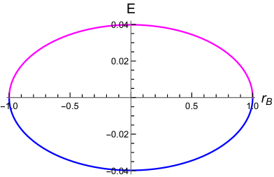
Figure 5: Plot of $E$ (left) and $C_{\phi_{B}}$ (right) as a function of radius $r_{B}$ for both cosmological (violet) and black hole (blue) systems. We have set $\phi_{r}=L=G_{2}=1$.

In total, combining the $\phi_{0}$ and $\phi$ terms (44), (45) and (47), the full on-shell Euclidean JT action for the cosmological system is

$$I_{\text{JT,c}}^{\text{E}}=-\frac{\phi_{r}}{4G_{2}}\frac{r_{B}^{2}}{L^{2}}-\frac{\phi_{0}}{4G_{2}}\;.$$ (48)

When evaluating at either horizon, we find the total action is minus the cosmological horizon entropy: $I_{\text{JT,c}}^{\text{E}}(r_{B}=\pm L)=-S_{\text{c}}$. From (47) we see the on-shell action can also be expressed as

$$I_{\text{JT,c}}^{\text{E}}=\beta E_{\text{c}}-S_{\text{c}}\,,$$ (49)

where $\beta$ is the inverse Tolman temperature (41), and the quasi-local energy $E_{\text{c}}$ and cosmological horizon entropy $S_{\text{c}}$ are

$$E_{\text{c}}=\frac{\phi_{r}}{8\pi G_{2}L}\sqrt{1-\frac{r_{B}^{2}}{L^{2}}}\,,\qquad\qquad S_{\text{c}}=\frac{\phi_{0}+\phi_{r}}{4G_{2}}\,.$$ (50)

Note that these expressions agree with the quasi-local energy in (39) and the JT entropy in (29). More precisely, these quantities can be obtained from the standard definitions

$$E=\left(\frac{\partial I_{\text{JT}}^{\text{E}}}{\partial\beta}\right)_{\phi_{B}}\,,\qquad S=\beta\left(\frac{\partial I_{\text{JT}}^{\text{E}}}{\partial\beta}\right)_{\phi_{B}}-I_{\text{JT}}^{\text{E}}\;,$$ (51)

where instead of the surface area of the boundary, the dilaton $\phi_{B}$ at $r=r_{B}$ is kept fixed. See Figure 5 for a plot of $E_{\text{c}}$ as a function of $r_{B}$ (violet curve).

The free energy follows directly from the on-shell Euclidean action

$$F_{\text{c}}=TI_{\text{JT,c}}^{\text{E}}=E_{\text{c}}-TS_{\text{c}}=-\frac{\phi_{r}}{8\pi G_{2}L}\frac{r_{B}^{2}/L^{2}}{\sqrt{1-\frac{r_{B}^{2}}{L^{2}}}}-\frac{\phi_{0}}{8\pi G_{2}L}\frac{1}{\sqrt{1-\frac{r_{B}^{2}}{L^{2}}}}\;.$$ (52)

The free energy diverges at the two horizons. Further, recall that $\phi_{0}>0$ in the full reduction model and $\phi_{0}=0$ in the half reduction model, such that the free energy is always less than or equal to zero, $F_{\text{c}}\leq 0$. Subtracting the free energy of pure dS₂ with a constant dilaton, $F_{0}=-TS_{\phi_{0}}$, the difference in free energies is always non-positive, $F_{\text{c}}-F_{0}\leq 0$, implying the nearly dS₂ geometry ($\phi_{r}\neq 0$) dominates the canonical ensemble over the pure dS₂ spacetime ($\phi_{r}=0$). Since the $F_{\text{c}}(r_{B})$ plot only has a single branch, there is no phase transition for the cosmological system in nearly dS₂ (see Figure 6).

         

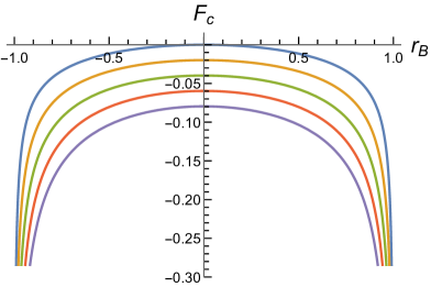
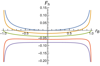
Figure 6: Plot of the free energy $F=E-TS$ as a function of radius $r_{B}$ in cosmological (left) and black hole (right) systems, for various values of $\phi_{0}$: $\{0,1/2,1,3/2,2\}=\{\text{blue},\text{orange},\text{green},\text{red},\text{purple}\}$. Here $\phi_{r}=L=G_{2}=1$.

Moreover, the heat capacity $C_{\phi_{B},\text{c}}$ for the cosmological system at constant $\phi_{B}$ is

$$C_{\phi_{B},\text{c}}=T\left(\frac{\partial S_{\text{c}}}{\partial T}\right)_{\phi_{B}}=\left(\frac{\partial E_{\text{c}}}{\partial T}\right)_{\phi_{B}}=-\frac{\phi_{r}}{4G_{2}}\left(1-\frac{r_{B}^{2}}{L^{2}}\right)<0\;.$$ (53)

The heat capacity is negative everywhere between the two horizons, $r_{\text{h}}=-L$ and $r_{\text{c}}=L$, and vanishes precisely at the horizons (see Figure 5). Hence, the cosmological system is always unstable for thermal fluctuations, which seems to be a general feature of cosmological horizons. For instance, in higher-dimensional SdS space the cosmological system defined between a boundary at radius $r=r_{B}$ and the cosmological horizon also has a negative heat capacity. This result appears to be in contradiction with Anninos:2017hhn , where the authors find a positive heat capacity for the cosmological horizon. However, the difference can be attributed to the choice of sign of the dilaton: they assume the dilaton is negative in dS₂, whereas we have taken it to be positive in the vicinity of the cosmological horizon.

Black hole system.

For completeness, consider the black hole system, where $r\in[-L,r_{B}]$, and $K=-\frac{r_{B}}{L^{2}}/\sqrt{1-\frac{r_{B}^{2}}{L^{2}}}$. The above analysis goes through similarly, where the on-shell Euclidean action is again

$$I^{\text{E}}_{\text{JT,h}}=\beta E_{\text{h}}-S_{\text{h}}\;,$$ (54)

except now the energy $E_{\text{h}}$ and entropy $S_{\text{h}}$ are given by

$$E_{\text{h}}=-\frac{\phi_{r}}{8\pi G_{2}L}\sqrt{1-\frac{r_{B}^{2}}{L^{2}}}\;,\quad S_{\text{h}}=\frac{\phi_{0}-\phi_{r}}{4G_{2}}\;.$$ (55)

At the two horizons, the total action is minus the black hole entropy: $I_{\text{JT,c}}^{\text{E}}(r_{B}=\pm L)=-S_{\text{h}}$. Consequently, the free energy $F_{\text{h}}$ and heat capacity $C_{\phi_{B},\text{h}}$ are

$$F_{\text{h}}=\frac{\phi_{r}}{8\pi G_{2}L}\frac{r_{B}^{2}/L^{2}}{\sqrt{1-\frac{r_{B}^{2}}{L^{2}}}}-\frac{\phi_{0}}{8\pi G_{2}L}\frac{1}{\sqrt{1-\frac{r_{B}^{2}}{L^{2}}}}\;,$$ (56)

and

$$C_{\phi_{B},\text{h}}=\frac{\phi_{r}}{4G_{2}}\left(1-\frac{r_{B}^{2}}{L^{2}}\right)>0\;.$$ (57)

Note that $C_{\phi_{B},\text{h}}$ is positive everywhere between the horizons at $r_{B}=\pm L$, and is zero at the horizons. Thus, the black hole system is stable with respect to thermal fluctuations (see blue curve on the right side in Figure 5). A similar result was obtained for AdS₂ black holes in Lemos:1996bq , where the system between the black hole horizon and the timelike boundary always has a positive heat capacity.

Further, in the half reduction model for $\phi_{0}=0$ we observe that the free energy is non-negative $F_{\text{h}}\geq 0$ everywhere, approaching positive infinity as one asymptotes to the horizons. In the full reduction model the free energy obeys $F_{\text{h}}\leq 0$ when $\phi_{0}\geq\frac{\phi_{r}r_{B}^{2}}{L^{2}}$. Subtracting the free energy of the pure dS₂ solution, $F_{0}=-TS_{\phi_{0}}$, the difference in free energies is always non-negative, $F_{\text{h}}-F_{0}\geq 0$, which means the pure dS₂ solution dominates the canonical ensemble for the black hole system. Finally, from Figure 6 for the $F_{\text{h}}(r_{B})$ plot and Figure 7 for the $F_{\text{h}}(T)$ plot we see there are no phase transitions for the black hole system.

         

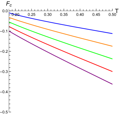
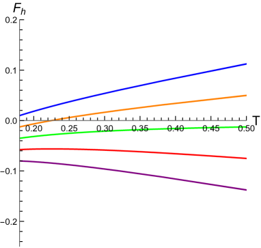
Figure 7: Plot of the free energy $F=E-TS$ as a function of the Tolman temperature for the cosmological (left) and black hole (right) systems, for various values of $\phi_{0}$: $\{0,1/2,1,3/2,2\}=\{\text{blue},\text{orange},\text{green},\text{red},\text{purple}\}$. We have set $\phi_{r}=L=G_{2}=1$.

3.3 Quasi-local Euler relation and first law

The quasi-local thermodynamic quantities are related to each other by the Euler equation (or Smarr formula) and obey a first law, as shown by York for a Schwarzschild black hole in York:1986it . In this section we derive both of these relations for de Sitter JT gravity using the Noether charge formalism Wald:1993nt ; Iyer:1994ys (see Pedraza:2021cvx or Appendix C for a summary).

Quasi-local Euler relation

In Liberati:2015xcp ; Jacobson:2018ahi ; Pedraza:2021cvx the Smarr formula was derived from the following integral identity

$$\int_{\Sigma}j_{\xi}=\oint_{\partial\Sigma}Q_{\xi}=\oint_{\mathcal{S}}Q_{\xi}+\oint_{\mathcal{H}}Q_{\xi}\;,$$ (58)

where $j_{\xi}$ is the Noether current 1-form associated with the Killing symmetry generated by $\xi$, and $Q_{\xi}$ is the associated Noether charge $0$-form, obeying the on-shell identity $j_{\xi}=dQ_{\xi}$. In our set-up, $\Sigma$ is a constant-$t$ surface in the static patch, and its boundary is given by $\partial\Sigma=\mathcal{S}\cup\mathcal{H}$, with $\mathcal{H}$ being the location of the bifurcation point of a Killing horizon (either the black hole or the cosmological horizon) and $\mathcal{S}$ is the intersection of $\Sigma$ and the timelike boundary $B$. The first equality in (58) is an application of Stokes’ theorem, and in the second equality the orientation of the Noether charge integral at $\mathcal{H}$ and $\mathcal{S}$ is taken to be outward. We now compute both sides of the integral identity explicitly for de Sitter JT gravity.

To evaluate the left-hand side we need the definition of the Noether current 1-form $j_{\xi}$

$$j_{\xi}\equiv\theta(\psi,\mathcal{L}_{\xi}\psi)-\xi\cdot L_{\text{JT}}\,.$$ (59)

The symplectic potential 1-form of classical JT gravity vanishes when evaluated on the Lie derivative along the Killing vector $\xi$, i.e., $\theta(\psi,\mathcal{L}_{\xi}\psi)=0$. The (Lorentzian) JT Lagrangian 2-form $L_{\text{JT}}$ is on shell given by

$$L_{\text{JT}}=\frac{\epsilon}{16\pi G_{2}}\left[(\phi_{0}+\phi)R-\frac{2}{L^{2}}\phi\right]=\frac{\epsilon\phi_{0}}{8\pi G_{2}L^{2}}\,,$$ (60)

with $\epsilon$ being the spacetime volume form, and we inserted the dilaton equation of motion $R=2/L^{2}$ in the last equality. Therefore, the left-hand side of the integral relation is

$$\int_{\Sigma}j_{\xi}=-\frac{\phi_{0}}{8\pi G_{2}L^{2}}\int_{\Sigma}\xi\cdot\epsilon=-\frac{\phi_{0}\Lambda}{8\pi G_{2}}\Theta_{\xi}\,,$$ (61)

Following Jacobson:2018ahi ; Pedraza:2021cvx , we introduced the “Killing volume” $\Theta_{\xi}$, which is defined as the proper volume (length in 2D) of $\Sigma$ locally weighted by the norm of $\xi$,

$$\Theta_{\xi}=\int_{\Sigma}|\xi|d\ell\;.$$ (62)

Here we have written $\xi\cdot\epsilon\,|_{\Sigma}=|\xi|d\ell$, where $d\ell$ is the infinitesimal proper length $d\ell=dr/\sqrt{f(r)}$ and the norm is $|\xi|=\sqrt{f(r)}$. Thus, for the cosmological system the Killing volume is given by $\Theta_{\xi,\text{c}}=L-r_{B}$, whereas for the black hole system we have $\Theta_{\xi,\text{h}}=L+r_{B}.$

On the right-hand side of the integral identity (58) we use the expression for the Noether charge in JT gravity, cf. Eq. (222),

$$Q_{\xi}^{\text{JT}}=-\frac{1}{16\pi G_{2}}\epsilon_{\mu\nu}\left[(\phi+\phi_{0})\nabla^{\mu}\xi^{\nu}+2\xi^{\mu}\nabla^{\nu}(\phi+\phi_{0})\right]\;,$$ (63)

where $\epsilon_{\mu\nu}|_{\partial\Sigma}=(n_{\mu}u_{\nu}-n_{\nu}u_{\mu})$ is the binormal of $\partial\Sigma$, satisfying $\epsilon_{\mu\nu}\epsilon^{\mu\nu}=-2$, and we used that the volume form is $\epsilon_{\partial\Sigma}=1$ in 2D. At the bifurcation point $\mathcal{H}$ we have $\xi|_{\mathcal{H}}=0$ and $\nabla_{\mu}\xi_{\nu}|_{\mathcal{H}}=-\kappa\epsilon_{\mu\nu}$. Hence,

$$\oint_{\mathcal{H}}Q_{\xi}=-\frac{\kappa}{8\pi G_{2}}(\phi_{0}+\phi_{\mathcal{H}})\,,$$ (64)

which is equal to minus the Gibbons–Hawking temperature $T_{\text{GH}}=\kappa/2\pi$ times the horizon entropy $S_{\mathcal{H}}$ (which is the same everywhere on the Killing horizon $H$). Meanwhile, since the boundary ${\mathcal{S}}$ is defined as the intersection of $\Sigma$ (with unit normal $u^{\mu}=\xi^{\mu}/N$) and $B$ (with unit normal $n^{\mu}$) we have $n\cdot u|_{\mathcal{S}}=0$ or $n\cdot\xi|_{\mathcal{S}}=0$, hence the Noether charge at $\mathcal{S}$ is

$$Q_{\xi}\big{|}_{\mathcal{S}} =-\frac{1}{8\pi G_{2}}\left[\frac{1}{2}(\phi+\phi_{0})(-NK-n^{\mu}\nabla_{\mu}N)+Nn^{\nu}\nabla_{\nu}(\phi+\phi_{0})\right]\Big{|}_{\mathcal{S}}$$ (65)

$$=-\frac{1}{8\pi G_{2}}\Big{[}-Nn^{\mu}a_{\mu}(\phi_{0}+\phi)+Nn^{\nu}\nabla_{\nu}(\phi_{0}+\phi)\Big{]}\Big{|}_{\mathcal{S}}\;.$$

In the first equality we used $-u\cdot\xi=N$ and $-u_{\nu}\nabla^{\mu}\xi^{\nu}=\nabla^{\mu}N$, where $N=|\xi|$ is the norm (36) of the Killing vector $\xi$. Further, we inserted the extrinsic curvature of $B$, $K_{\mu\nu}=2\nabla_{(\mu}n_{\nu)}$, and the relation $K_{\mu\nu}=K\gamma_{\mu\nu}$ in two dimensions. In the second equality we employed the trace of the extrinsic curvature $K=\frac{1}{N}n^{\mu}\nabla_{\mu}N=n^{\mu}a_{\mu}$, which is equal to the normal component of the acceleration vector $a^{\mu}=u^{\nu}\nabla_{\nu}\xi^{\mu}=\frac{1}{N}\nabla^{\mu}N$.

Thus, inserting (61), (64) and (65) into the integral identity (58) we arrive to the following relation

$$-\frac{\phi_{0}\Lambda}{8\pi G_{2}}\Theta_{\xi}=-\frac{\kappa}{8\pi G_{2}}(\phi_{0}+\phi_{H})+\frac{Nn^{\mu}a_{\mu}}{8\pi G_{2}}(\phi_{0}+\phi_{B})-\frac{N}{8\pi G_{2}}n^{\mu}\nabla_{\mu}\phi\;.$$ (66)

Our notation above reflects that $\phi_{\mathcal{S}}=\phi(r_{B})=\phi_{B}$, and similarly $\phi_{\mathcal{H}}=\phi(r_{H})=\phi_{H}$. Dividing by $N$ yields the quasi-local Euler relation

$$E=TS_{H}-\sigma(\phi_{0}+\phi_{B})-\frac{\phi_{0}\Lambda}{8\pi G_{2}N}\Theta_{\xi}\;,$$ (67)

where $E$ is the quasi-local energy (39), $T$ is the Tolman temperature (37), $S_{H}$ is the horizon entropy (29), and we introduced the “surface pressure” $\sigma$

$$\sigma=\frac{n^{\mu}a_{\mu}}{8\pi G_{2}}=\pm\frac{1}{8\pi G_{2}}\frac{r_{B}/L^{2}}{\sqrt{1-\frac{r_{B}^{2}}{L^{2}}}}\,.$$ (68)

The plus sign applies to the cosmological system, while the minus sign is associated to the black hole system. We emphasize that the quasi-local Euler relation holds for both thermodynamic systems. We can compare the definition of the surface pressure in JT gravity to the standard definition of surface pressure in $d$-dimensional Einstein gravity: $\sigma=\frac{1}{(d-2)8\pi G_{d}}(-k^{\alpha\beta}+(n^{\mu}a_{\mu}+k)\sigma^{\alpha\beta})\sigma_{\alpha\beta}$, where $\sigma_{\alpha\beta}$ is the induced metric on $\mathcal{S}$ Brown:1992br . Setting the extrinsic curvature $k^{\alpha\beta}$ of the codimension-two surface $\mathcal{S}$ to zero, since the surface is just a point in 2D, and using $\sigma^{\alpha\beta}\sigma_{\alpha\beta}=d-2$, we recover the definition in (68).

Notice that in the half reduction model the Killing volume term in the Euler relation (67) vanishes since $\phi_{0}=0$. In fact, the Euler relation splits into two separate equations

$$E=TS_{\phi_{H}}-\sigma\phi_{B}\;,\qquad 0=TS_{\phi_{0}}-\sigma\phi_{0}-\frac{\phi_{0}\Lambda}{8\pi G_{2}N}\Theta_{\xi}\,.$$ (69)

Hence, in the half reduction model the second equation is trivial and the Euler relation reduces to the first expression. The first equation can be interpreted as the Euler relation for nearly dS₂ with $\phi_{0}=0$ but $\phi_{r}\neq 0$, while the second equation is the Euler relation for dS₂ with a constant dilaton $\phi_{0}\neq 0$ but $\phi_{r}=0$. The two relations in (69) can be verified explicitly using the expressions for the thermodynamic variables in static patch coordinates.

In the limit that the thermodynamic systems become the full static patch, i.e., $r_{B}\to\pm L$ for the respective systems, the product $Nn^{\mu}a_{\mu}$ in Eq. (66) is equal to minus the surface gravity

$$Nn^{\mu}a_{\mu}\to-\kappa\qquad\text{as}\qquad r_{B}\to r_{\text{h,c}}\,.$$ (70)

This is equivalent to the standard definition of surface gravity $\kappa=\lim_{H}(Na)$ where the magnitude of the acceleration is defined as $a=\sqrt{a^{\mu}a_{\mu}}$. Further, we have $N\to 0$, $E\to 0$, and $\frac{1}{4G_{2}}(\phi_{0}+\phi_{B})\to S_{\text{h,c}}$ as $r_{B}\to r_{\text{h,c}}.$ Hence, if we take the limit of (66) to the full static patch, then the Euler relation becomes

$$0=T_{\text{GH}}S_{\text{h}}+T_{\text{GH}}S_{\text{c}}-\frac{\phi_{0}\Lambda}{8\pi G_{2}}\Theta_{\xi}\,,$$ (71)

where the Killing volume (62) is now defined between the cosmological and black hole horizon, $\Theta_{\xi}=\int_{-L}^{L}dr=2L$. Equivalently, for the full static patch the two separate equations in (69) become

$$0=T_{\text{GH}}S_{\phi_{\text{h}}}+T_{\text{GH}}S_{\phi_{\text{c}}}\,,\quad\ \quad 0=2T_{\text{GH}}S_{\phi_{0}}-\frac{\phi_{0}\Lambda}{8\pi G_{2}}\Theta_{\xi}\,.$$ (72)

We anticipated the first relation in Eq. (30), and the second equation is the Euler relation for the dimensionally reduced extremal Nariai solution.

Quasi-local first law

The quasi-local first law for both the cosmological and black hole system is

$$dE=TdS_{H}-\sigma d\phi_{B}\,.$$ (73)

This follows from the coordinate expressions for the relevant thermodynamic quantities. In particular, it can be checked that the Tolman temperature (37) and surface pressure (68) satisfy

$$T=\left(\frac{\partial E}{\partial S_{H}}\right)_{\phi_{B}}\,,\qquad\sigma=-\left(\frac{\partial E}{\partial\phi_{B}}\right)_{S_{H}}\,.$$ (74)

Ultimately, these relations contain the same content as the quasi-local first law (73). Further, we point out that the first law follows from the dimensional reduction of the quasi-local Euler relation for Schwarzschild-de Sitter, $dE=TdS_{H}-\sigma dA$, because the area of $\mathcal{S}$ becomes equal to $\phi_{B}$ after a spherical reduction.

In addition, although the relations (74) can be checked in terms of static patch coordinates, a covariant derivation of the quasi-local first law is desired. In fact, the first law follows also from varying the Smarr relation (58), which leads to the fundamental variational integral identity Wald:1993nt ; Iyer:1994ys

$$\int_{\Sigma}\omega(\psi,\delta\psi,\mathcal{L}_{\xi}\psi)=\oint_{\partial\Sigma}[\delta Q_{\xi}-\xi\cdot\theta(\psi,\delta\psi)]\;,$$ (75)

where $\omega(\psi,\delta_{1}\psi,\delta_{2}\psi)\equiv\delta_{1}\theta(\psi,\delta_{2}\psi)-\delta_{2}\theta(\psi,\delta_{1}\psi)$ is the symplectic current 1-form, cf. Eq. (219) for an explicit expression in dilaton gravity. Since $\mathcal{L}_{\xi}\psi=0$, and the symplectic current is linear in $\mathcal{L}_{\xi}\psi$, the left-hand side of (75) is zero. The right-hand side of (75) splits into an integral at the bifurcation point $\mathcal{H}$ of the Killing horizon (either the black hole or the cosmological horizon)

$$\oint_{\mathcal{H}}[\delta Q_{\xi}-\xi\cdot\theta(\psi,\delta\psi)]=-\frac{\kappa}{8\pi G_{2}}\delta\phi_{H}\,,$$ (76)

where we used $\xi|_{\mathcal{H}}=0$ and Eq. (64), and an integral at the intersection point $\mathcal{S}=\Sigma\cap B$. The latter can be computed by evaluating the variation of the Noether charge (65)

$$\delta Q_{\xi}|_{\mathcal{S}}=\frac{1}{8\pi G_{2}}\delta\Big{(}Nn^{\mu}a_{\mu}(\phi_{0}+\phi_{B})\Big{)}+\delta(EN)\,,$$ (77)

and the symplectic potential at $B$, cf. Eq. (C.6) of Pedraza:2021cvx (ignoring the $dC$ contribution since $\xi\cdot dC=\mathcal{L}_{\xi}C-d(\xi\cdot C)$ vanishes after integration over $\mathcal{S}$),

$$\theta(\psi,\delta\psi)|_{B} =\frac{\epsilon_{B}}{8\pi G_{2}}\Big{(}K\delta\phi_{B}+\frac{1}{2}\gamma^{\mu\nu}n^{\alpha}\nabla_{\alpha}\phi\delta\gamma_{\mu\nu}\Big{)}-\frac{1}{8\pi G_{2}}\delta\Big{(}\epsilon_{B}K(\phi_{0}+\phi_{B})\Big{)}$$ (78)

$$=-\epsilon_{B}\frac{E}{N}\delta N-\frac{\epsilon_{B}}{8\pi G_{2}}\left[(\phi_{0}+\phi_{B})\delta(n^{\mu}a_{\mu})+\frac{1}{N}n^{\mu}a_{\mu}(\phi_{0}+\phi_{B})\delta N\right].$$

Here, we inserted $K=n^{\mu}a_{\mu}$ , $\frac{1}{2}\gamma^{\mu\nu}\delta\gamma_{\mu\nu}=\delta N/N$, $E=-\frac{1}{8\pi G_{2}}n^{\alpha}\nabla_{\alpha}\phi$, and $\delta\epsilon_{B}=(\frac{1}{2}\gamma^{\mu\nu}\delta\gamma_{\mu\nu})\epsilon_{B}$ in the second equality. Using $\xi\cdot\epsilon_{B}=-N$ and combining (77) and (78) we find

$$\oint_{\mathcal{S}}\left[\delta Q_{\xi}-\xi\cdot\theta(\psi,\delta\psi)\right]=N\delta E+\frac{N}{8\pi G_{2}}n^{\mu}a_{\mu}\delta\phi_{B}\;.$$ (79)

Substituting (76), and (79) into (75) yields the covariant relation

$$\delta E=\frac{\kappa}{8\pi G_{2}N}\delta\phi_{H}-\sigma\delta\phi_{B}\;,$$ (80)

recovering the quasi-local first law (73).

Multiplying the quasi-local first law by the norm $N$ and taking the limit $r_{B}\to\pm L$, such that the thermodynamic system becomes the full static patch, we find

$$0=T_{\text{GH}}\delta S_{\text{c}}+T_{\text{GH}}\delta S_{\text{h}}\;,$$ (81)

since $NT=T_{\text{GH}}$, and $N\delta E\to 0$ and $N\sigma\to-\frac{1}{4G_{2}}T_{\text{GH}}$ in this limit. We recognize this as the 2D analog of the global first law (22) for Schwarzschild-de Sitter black holes. Note that this global first law only holds in the full reduction model of JT gravity. In contrast, in the half reduction model, when we take the limit where the thermodynamic system becomes the full patch, such that $r_{B}\to 0$ and $N\to 1$, the energy contribution is non-vanishing while the surface pressure (68) tends to zero. Consequently, in the half reduction model we attain the following “global” first law

$$\delta E=T_{\text{GH}}\delta S_{H}\;,$$ (82)

valid for either the cosmological or black hole system. In this case, for $r_{B}=0$ the energy is $E=\pm\frac{\phi_{r}}{8\pi G_{2}L}=T_{\text{GH}}S_{H}$.

The covariant derivation of the first law (80) may be generalized by including classical matter contributions, where the variation of the matter Hamiltonian $H_{\xi}$ is characterized by the matter energy-momentum tensor $T_{\mu\nu}$ and can be cast as $\delta H_{\xi}=-\int_{\Sigma}\delta({T_{\mu}}^{\nu})\xi^{\mu}\epsilon_{\nu}$ Jacobson:2018ahi . The quasi-local first law with a matter Hamiltonian variation reads

$$\delta E=\frac{\kappa}{8\pi G_{2}N}\delta\phi_{H}-\sigma\delta\phi_{B}+\delta H_{\xi}\;,$$ (83)

In the limit $r_{B}\to\pm L$, the global first laws (81) and (82) are appropriately modified.

3.4 Including semi-classical backreaction

A notable feature of JT gravity is that the effects of backreaction are fixed by the two-dimensional Polyakov action capturing the contributions of the conformal anomaly Polyakov:1981rd , in the semi-classical limit. Here we solve the problem of backreaction in de Sitter JT gravity and derive the semi-classical extension of the first law. In particular, we will find that the classical entropy is replaced by the semi-classical Wald entropy, which is equal to the generalized entropy, as we will discuss. Our treatment here largely follows the recent work Pedraza:2021cvx .

3.4.1 Vacuum states and generalized entropy

Semi-classical JT gravity in de Sitter space is described by minimally coupling the classical JT action (found from the full reduction) (26) to a dynamical two-dimensional conformal field theory $I_{\text{CFT}}$ of central charge $c$. Adding $I_{\text{CFT}}$ makes the semi-classical model an effective theory; unlike the classical action, the 2D CFT action does not follow from a dimensional reduction. Including $I_{\text{CFT}}$ modifies the classical equations of motion (12) by semi-classical effects

$$\frac{1}{8\pi G_{2}}\left(g_{\mu\nu}\Box-\nabla_{\mu}\nabla_{\nu}+\frac{1}{L^{2}}g_{\mu\nu}\right)\phi=\langle T_{\mu\nu}^{\text{CFT}}\rangle\;,$$ (84)

where $\langle T_{\mu\nu}^{\text{CFT}}\rangle\equiv-\frac{2}{\sqrt{-g}}\frac{\delta I_{\text{CFT}}}{\delta g^{\mu\nu}}$ is the expectation value of the stress-energy tensor $T_{\mu\nu}^{\text{CFT}}$ with respect to some unspecified quantum state $|\Psi\rangle$.

The conformal matter thus backreacts on the classical solution. To study the problem of backreaction consistently, we work in the large-$c$ limit such that $I_{\text{CFT}}$ is given by the non-local 1-loop Polyakov action $I_{\text{Poly}}$ Polyakov:1981rd . This 1-loop action can be put into a localized form by introducing a massless auxiliary scalar field $\chi$, modelling the 2D CFT, such that

$$I_{\text{Poly}}=-\frac{c}{24\pi}\int_{\mathcal{M}}d^{2}x\sqrt{-g}\left[(\nabla\chi)^{2}+\chi R\right]-\frac{c}{12\pi}\int_{\partial\mathcal{M}}dt\sqrt{-h}\chi K\;.$$ (85)

The boundary contribution we have included is a GHY term such that the localized 1-loop action has a well-posed variational problem. The equation of motion for $\chi$ is

$$2\Box\chi=R\;,$$ (86)

whose formal solution $\chi=\frac{1}{2}\int d^{2}y\sqrt{-g(y)}G(x,y)R(y)$ puts the local action (85) into its original non-local form. From the action (85), the semi-classical gravitational field equations are given by (84) where $\langle T_{\mu\nu}^{\text{CFT}}\rangle$ is now replaced by

$$\langle T_{\mu\nu}^{\chi}\rangle=\frac{c}{12\pi}\left[(g_{\mu\nu}\Box-\nabla_{\mu}\nabla_{\nu})\chi+(\nabla_{\mu}\chi)(\nabla_{\nu}\chi)-\frac{1}{2}g_{\mu\nu}(\nabla\chi)^{2}\right]\;.$$ (87)

Using the equation of motion for $\chi$ (86), it is easy to show $\langle T^{\chi}_{\mu\nu}\rangle$ has the well-known conformal anomaly

$$g^{\mu\nu}\langle T^{\chi}_{\mu\nu}\rangle=\frac{c}{24\pi}R\;.$$ (88)

In Christensen:1977jc it was recognized that in two dimensions the conformal anomaly captures all 1-loop quantum effects and the full backreaction.

Crucially, since the Polyakov action (85) does not directly couple to the dilaton $\phi$, it does not alter the dilaton equation of motion (13) and the background geometry remains exact $\text{dS}_{2}$. The classical solution of $\phi$ will be modified due to backreaction, but in the case of interest, $\phi$ will only be shifted by a constant proportional to $cG_{2}$, as in the $\text{AdS}_{2}$ model.

To proceed with the semi-classical analysis, we must specify the vacuum state of the quantum matter. We accomplish this as follows. First, we work in the conformal gauge, $d\ell^{2}=-e^{2\rho(y^{+},y^{-})}dy^{+}dy^{-}$, where $(y^{+},y^{-})$ are some null conformal coordinates. One finds the solution for the auxiliary field $\chi$ to be

$$\chi=-\rho+\xi(y^{+},y^{-})\;,\quad\text{with}\quad\Box\xi=0\quad\Rightarrow\quad\xi(y^{+},y^{-})=\xi_{+}(y^{+})+\xi_{-}(y^{-})\;.$$ (89)

The $\xi_{\pm}(y^{\pm})$ constitute functions $t_{\pm}(y^{\pm})$,

$$t_{+}(y^{+})=\partial^{2}_{+}\xi_{+}-(\partial_{+}\xi_{+})^{2}\;,\quad t_{-}(y^{-})=\partial_{-}^{2}\xi_{-}-(\partial_{-}\xi_{-})^{2}\;,$$ (90)

which characterize the normal-ordered stress-tensor

$$\langle\Psi|:T_{\pm\pm}^{\chi}(y^{\pm}):|\Psi\rangle=-\frac{c}{12\pi}t_{\pm}(y^{\pm})\;.$$ (91)

From the definition of normal ordering, $:T_{\pm\pm}^{\chi}:\equiv T^{\chi}_{\pm\pm}(y^{\pm})-\langle 0_{y}|T^{\chi}_{\pm\pm}(y^{\pm})|0_{y}\rangle$, the vacuum state $|0_{y}\rangle$ with respect to the positive frequency modes in coordinates $y^{\pm}$ is the state obeying

$$\langle 0_{y}|:T^{\chi}_{\pm\pm}(y^{\pm}):|0_{y}\rangle=0\;\;\Leftrightarrow\;\;t_{\pm}(y^{\pm})=0\;.$$ (92)

Moreover, the transformation properties of $\rho$ and $\xi$ reveal that the normal-ordered stress tensor obeys an anomalous transformation law under a conformal transformation $y^{\pm}\to x^{\pm}(y^{\pm})$, such that

$$\langle 0_{y}|:T^{\chi}_{\pm\pm}(x^{\pm}):|0_{y}\rangle=-\frac{c}{24\pi}\{y^{\pm},x^{\pm}\}\;,$$ (93)

and

$$\langle 0_{y}|T_{\pm\pm}^{\chi}(x^{\pm})|0_{y}\rangle=\langle 0_{x}|T_{\pm\pm}^{\chi}(x^{\pm})|0_{x}\rangle-\frac{c}{24\pi}\{y^{\pm},x^{\pm}\}\;.$$ (94)

Here $|0_{x}\rangle$ is the vacuum defined with respect to the positive frequency modes in the $x^{\pm}$ coordinate system, and $\{y^{\pm},x^{\pm}\}$ denotes the Schwarzian derivative

$$\{y^{\pm},x^{\pm}\}\equiv\frac{(y^{\pm})^{\prime\prime\prime}}{(y^{\pm})^{\prime}}-\frac{3}{2}\left(\frac{(y^{\pm})^{\prime\prime}}{(y^{\pm})^{\prime}}\right)^{2}\;,\quad(y^{\pm})^{\prime}\equiv\frac{dy^{\pm}}{dx^{\pm}}\;.$$ (95)

The central lesson of (93) is that observers in different coordinates will experience the same vacuum differently.

Static and Bunch–Davies vacua

Let us now be more explicit and consider two vacuum states of interest, the static (S) and Bunch–Davies (BD) vacua. We do this by choosing two conformally related sets of null coordinates. The static vacuum $|\text{S}\rangle$ characterizes the state of a static observer confined to the static patch of $\text{dS}_{2}$, i.e., $(v,u)$ coordinates (33). The static vacuum is conformally related to the Rindler vacuum in Minkowski space, and analogous to the Boulware vacuum of a black hole. The Bunch–Davies vacuum $|\text{BD}\rangle$ characterizes the state of an observer in Kruskal-like coordinates $(V,U)$, given in (35). It is conformally related to the global Minkowski vacuum state, and analogous to the Hartle-Hawking state of a black hole in thermal equilibrium with its Hawking radiation.

By the normal-ordered relation (92), we have

$$\langle\text{S}|:T_{vv}^{\chi}:|\text{S}\rangle=\langle\text{S}|:T_{uu}^{\chi}:|\text{S}\rangle=0\quad\Leftrightarrow\quad t_{v}(v)=t_{u}(u)=0\;,$$ (96)

and

$$\langle\text{BD}|:T_{VV}^{\chi}:|\text{BD}\rangle=\langle\text{BD}|:T_{UU}^{\chi}:|\text{BD}\rangle=0\quad\Leftrightarrow\quad t_{V}(V)=t_{U}(U)=0\;.$$ (97)

Moreover, it is straightforward to show that for the static vacuum,

$$\langle\text{S}|:T^{\chi}_{VV}:|\text{S}\rangle=\langle\text{S}|T^{\chi}_{VV}|\text{S}\rangle=-\frac{c}{48\pi V^{2}}\;,\quad\langle\text{S}|:T^{\chi}_{UU}:|\text{S}\rangle=\langle\text{S}|T^{\chi}_{\text{UU}}|\text{S}\rangle=-\frac{c}{48\pi U^{2}}\;,$$ (98)

$$\langle\text{S}|T^{\chi}_{uu}|\text{S}\rangle=\langle\text{S}|T^{\chi}_{vv}|\text{S}\rangle=-\frac{c}{48\pi L^{2}}\;,$$ (99)

and for the Bunch–Davies vacuum,

$$\langle\text{BD}|:T^{\chi}_{uu}:|\text{BD}\rangle=\langle\text{BD}|:T^{\chi}_{vv}:|\text{BD}\rangle=\frac{c\pi}{12}T^{2}_{\text{GH}}\;,$$ (100)

$$\langle\text{BD}|T^{\chi}_{VV}|\text{BD}\rangle=\langle\text{BD}|T^{\chi}_{UU}|\text{BD}\rangle=\langle\text{BD}|T^{\chi}_{uu}|\text{BD}\rangle=\langle\text{BD}|T^{\chi}_{vv}|\text{BD}\rangle=0\;.$$ (101)

To summarize, from (98) we see the static vacuum state expectation value of the renormalized stress-tensor in Kruskal coordinates becomes singular on the past and future cosmological horizons ($V=0$ and $U=0$). In static null coordinates $(v,u)$, we find a negative energy density, (99). This behavior is analogous to the Casimir energy of the Boulware state in an eternal black hole background. Alternatively, an observer in the static patch will see the Bunch–Davies vacuum as a thermal state at the Gibbons–Hawking temperature, cf. (100). More precisely, a static observer detects a left and right flux of particles at the same temperature $T_{\text{GH}}$, such that the static patch of $\text{dS}_{2}$ is a thermal system at temperature $T_{\text{GH}}$, and $|\text{BD}\rangle$ restricted to the static patch is a thermal equilibrium state. Indeed, the Bunch–Davies state can be written as a thermofield double state with respect to energy eigenstates $|E_{i}\rangle_{L,R}$ characterizing left and right static patches

$$|\text{BD}\rangle=\frac{1}{Z}\sum_{i}e^{-\beta E_{i}/2}|E_{i}\rangle_{L}|E_{i}\rangle_{R}\,.$$ (102)

Tracing out the degrees of freedom of, say, the left static patch, the reduced density matrix is a thermal Gibbs state

$$\rho_{\text{BD}}^{R}=\text{tr}_{L}\rho_{\text{BD}}=\frac{1}{Z}\sum_{i}e^{-\beta E_{i}}|E_{i}\rangle_{R}\langle E_{i}|_{R}\;.$$ (103)

In the following we will only work with the Bunch–Davies vacuum state precisely because of its thermal nature.

Wald entropy is generalized entropy

Since it has a temperature, it is natural to assign a thermodynamic entropy to the cosmological horizon. Given the semi-classical JT action, we do this by following the Noether charge method and computing the Wald entropy Wald:1993nt , including quantum backreaction. One finds

$$S_{\text{Wald}}=\frac{1}{4G_{2}}(\phi_{0}+\phi_{H})-\frac{c}{6}\chi_{H}\;,$$ (104)

where the backreacted solutions for $\phi$ and $\chi$ are evaluated on the horizon. With respect to the Bunch–Davies vacuum, a state in thermal equilibrium, we justifiably interpret the Wald entropy as a thermodynamic entropy.

The first term in the Wald entropy (104) is the usual “area” law in the Gibbons–Hawking entropy formula for de Sitter space. Assuming the conformal matter is in the BD vacuum, the backreacted $\phi$ is the classical solution shifted by an unimportant constant proportional to $cG_{2}$. The second term is purely due to the 1-loop Polyakov action, entirely encoding the entropy due to the CFT represented by $\chi$. In fact, as recently argued in Pedraza:2021cvx , this second term is exactly equal to the von Neumann entropy $S_{\text{vN}}$ of a 2D CFT restricted to a single interval $[(y^{+}_{1},y^{-}_{1}),(y^{+}_{2},y^{-}_{2})]$ on a two-dimensional background $d\ell^{2}=-e^{2\rho(y^{+},y^{-})}dy^{+}dy^{-}$ (cf. Fiola:1994ir )

$$S_{\text{vN}}=\frac{c}{6}\log\left[\frac{1}{\delta_{1}\delta_{2}}(y^{+}_{2}-y^{+}_{1})(y^{-}_{2}-y^{-}_{1})e^{\rho(y^{+}_{1},y^{-}_{1})}e^{\rho(y^{+}_{2},y^{-}_{2})}\right]\;.$$ (105)

Here $\delta_{1,2}$ are independent UV regulators which resolve divergences arising from evaluating $S_{\text{vN}}$ at the endpoints of the interval. With respect to the Bunch–Davies vacuum, we can show explicitly that the general backreacted solution for $\chi$ in global coordinates $(V,U)$ (35) takes precisely the form of $S_{\text{vN}}$

$$-\frac{c}{6}\chi =\frac{c}{12}\log\left[\frac{16}{\left(1-\frac{U_{1}V_{1}}{L^{2}}\right)^{2}\left(1-\frac{U_{2}V_{2}}{L^{2}}\right)^{2}}\right]+\frac{c}{12}\log\left[\frac{1}{\delta_{1}^{2}\delta_{2}^{2}}(U_{2}-U_{1})^{2}(V_{2}-V_{1})^{2}\right]$$ (106)

$$=S_{\text{vN}}^{\text{BD}}\;.$$

Here the CFT is restricted to the interval $[(U_{1},V_{1}),(U_{2},V_{2})]$. The entropy is generically time-dependent, despite the spacetime being static. This form of the von Neumann entropy is for a single interval inside the shaded regions in Figure 3; it does not give the entropy for an interval with endpoints in different hyperbolic patches, as could be the case for the full reduction model. This scenario is dealt with by performing the continuation (195) on one of the endpoints.

While we explicitly computed (106), the result $S_{\text{vN}}=-\frac{c}{6}\chi$ holds for any 2D gravity theory coupled to a large $c$ CFT and with respect to any vacuum state Pedraza:2021cvx . This primarily follows from the fact that generically $\chi=-\rho+\xi$, as in (89), and imposing $\chi$ obeys Dirichlet boundary conditions. Thus, the general solution for $\chi$ is proportional to the von Neumann entropy (105) of a 2D CFT in vacuum reduced to a single interval in a curved background. The semi-classical Wald entropy (104), then, is exactly equal to the generalized entropy

$$S_{\text{Wald}}=S_{\text{gen}}\;.$$ (107)

Relating $S_{\text{Wald}}$ to $S_{\text{gen}}$ was previously hinted at but not realized in Myers:1994sg in the case of 2D flat space; the observation (106) has seemingly only been recognized in Pedraza:2021cvx . It is worth pointing out that normally the Wald entropy represents only the gravitational contribution to the generalized entropy, while the matter entropy is solely due to the von Neumann entropy of the quantum fields living on the background. In the context of two-dimensional gravity, however, the entire effect of conformal matter living on the background is encoded in the 1-loop Polyakov action, for which we may apply the Wald formalism to compute the entropy. We do not expect this observation to be true in higher dimensions as the trace anomaly does not provide complete information of the matter fields.

A comment on CFTs in the half vs. full reduction models

As emphasized in Section 2, the half reduction model of de Sitter JT gravity leads to a $\text{dS}_{2}$ geometry that is restricted, due to the fact that the dilaton $\Phi\geq 0$. No such restriction occurs in the full reduction model. Here the quantum matter is described by a two-dimensional CFT in both versions of JT gravity. This is not a natural viewpoint for the half reduction because the CFT does not see the full space: the half reduction effectively restricts the CFT from a cylinder to the half plane. Therefore, it is more natural to describe the quantum matter as a CFT in the full reduction model, while in the half reduction one should probably consider a boundary CFT.

3.4.2 Semi-classical thermodynamics

Briefly, let us now derive the semi-classical extension of the quasi-local Euler relation and first law of thermodynamics in dS₂. We again use Noether charge techniques, following Pedraza:2021cvx . In principle, we could have performed an on-shell Euclidean action analysis when $\chi$ is static, as we did in the classical case. However, for a time-dependent $\chi$ this approach is conceptually and computationally challenging, and a covariant analysis is desired.

Semi-classical quasi-local Euler relation

We use the integral identity (58), where now we include the Noether charge and current associated with the 1-loop Polyakov action. We begin with the right-hand side of (58). The Noether charge $Q_{\xi}^{\chi}$ for the auxiliary field $\chi$ is

$$Q_{\xi}^{\chi}=\frac{c}{24\pi}\epsilon_{\mu\nu}[\chi\nabla^{\mu}\xi^{\nu}+2\xi^{\mu}\nabla^{\nu}\chi]\;.$$ (108)

Evaluating this at the bifurcate point $\mathcal{H}$ of the Killing horizon $H$ yields

$$\oint_{\mathcal{H}}Q_{\xi}^{\chi}=\frac{\kappa c}{12\pi}\chi_{\mathcal{H}}\;,$$ (109)

where $\chi_{\mathcal{H}}=\chi_{H}$. Clearly this is equal to the temperature times the semi-classical correction to the Wald entropy due to $\chi$ (104). Meanwhile, the Noether charge $Q_{\xi}^{\chi}$ associated to $\chi$ evaluated at $\mathcal{S}$ is

$$Q^{\chi}_{\xi}|_{\mathcal{S}}=\frac{c}{12\pi}\left(-Nn^{\mu}a_{\mu}\chi+Nn^{\nu}\nabla_{\nu}\chi\right)|_{\mathcal{S}}\;.$$ (110)

Note $\chi_{\mathcal{S}}$ is not the same as $\chi_{B}$ when $\chi$ is time dependent. Consider now the left-hand side of the relation (58), where the only new contribution arises from $\chi$. The associated Noether current 1-form $j_{\xi}^{\chi}$ on shell is given by

$$j_{\xi}^{\chi}|_{\Sigma}=-\xi\cdot L_{\text{Poly}}=\frac{c}{12\pi L^{2}}\left[\chi+\frac{L^{2}}{2}(\nabla\chi)^{2}\right]\xi\cdot\epsilon\;,$$ (111)

where we used $\theta_{\chi}(\psi,\mathcal{L}_{\xi}\psi)|_{\Sigma}=0$, since $\chi$ is static at $\Sigma$ and $\mathcal{L}_{\xi}g_{\mu\nu}=0$, and the Polyakov Lagrangian 2-form $L_{\text{Poly}}$ is

$$L_{\text{Poly}}=-\frac{c}{24\pi}\epsilon[\chi R+(\nabla\chi)^{2}]\;.$$ (112)

Thus, analogous to (61), we may express the left-hand side of (58) in terms of a semi-classical “Killing volume” $\Theta^{\chi}_{\xi}$:

$$\int_{\Sigma}j_{\xi}^{\chi}=\frac{c\Lambda}{12\pi}\Theta_{\xi}^{\chi}\;,\quad\Theta_{\xi}^{\chi}\equiv\int_{\Sigma}\left(\chi+\frac{L^{2}}{2}(\nabla\chi)^{2}\right)\xi\cdot\epsilon\;.$$ (113)

Adding the semi-classical corrections (109), (110), and (113) to the classical Euler relation (66) yields the semi-classical quasi-local Euler relation for de Sitter JT gravity:

$$E=TS_{\text{gen},H}-\sigma\left((\phi_{0}+\phi_{B})-\frac{2G_{2}c}{3}\chi_{\mathcal{S}}\right)-\frac{\phi_{0}\Lambda}{8\pi G_{2}N}\Theta_{\xi}+\frac{c\Lambda}{12\pi N}\Theta_{\xi}^{\chi}\;.$$ (114)

Here $E$ refers to the sum of classical and semi-classical contributions to the energy, namely,

$$E=-\frac{1}{8\pi G_{2}}n^{\nu}\nabla_{\nu}\phi+\frac{c}{12\pi}n^{\nu}\nabla_{\nu}\chi=E_{\phi}+E_{\chi}\;.$$ (115)

The semi-classical quasi-local Euler relation (114) may be split into three equations. The first two involve $\phi_{r}$ and $\phi_{0}$, respectively, and are equivalent to the classical expressions in Eq. (69). The third equation is proportional to $c$ and is given by

$$E_{\chi}=TS_{\chi_{H}}+\frac{2G_{2}c}{3}\sigma\chi_{\mathcal{S}}+\frac{c\Lambda}{12\pi N}\Theta^{\chi}_{\xi}\;.$$ (116)

Further, in the limit the thermodynamic systems become the full static patch, in the full reduction we have that the quasi-local Smarr formula (114) becomes the semi-classical Euler relation

$$0=T_{\text{GH}}S_{\text{gen,h}}+T_{\text{GH}}S_{\text{gen,c}}-\frac{\phi_{0}\Lambda}{8\pi G_{2}N}\Theta_{\xi}+\frac{c\Lambda}{12\pi N}\Theta_{\xi}^{\chi}\;.$$ (117)

Semi-classical quasi-local first law

The semi-classical first law follows from the variational identity (75). Unlike the classical case, the left-hand side of (75) is generally non-zero solely due to the presence of the auxiliary field $\chi$. This is because the symplectic current 1-form with respect to the Polyakov action is (see Eq. (4.88) of Pedraza:2021cvx )

$$\omega_{\chi}(\psi,\delta\psi,\mathcal{L}_{\xi}\psi)|_{\Sigma}=-\frac{c}{24\pi}\epsilon_{\mu}\left[(g^{\mu\beta}g^{\alpha\nu}-g^{\mu\nu}g^{\alpha\beta})\nabla_{\nu}(\mathcal{L}_{\xi}\chi)\delta g_{\alpha\beta}-2\nabla^{\mu}(\mathcal{L}_{\xi}\chi)\delta\chi\right]\Big{|}_{\Sigma}\;,$$ (118)

where we used $\mathcal{L}_{\xi}g_{\mu\nu}=0$ and $\mathcal{L}_{\xi}\chi|_{\Sigma}=0$. This is non-zero because generally $\nabla_{\mu}(\mathcal{L}_{\xi}\chi)|_{\Sigma}\neq 0$. Moreover, we cannot explicitly evaluate the integral of the symplectic current over $\Sigma$. Thus, we express the left-hand side of (75) formally, via Hamilton’s equations, as the variation of the Hamiltonian associated to the $\chi$ field, generating evolution along the flow of $\xi$,

$$\delta H_{\xi}^{\chi}=\int_{\Sigma}\omega_{\chi}(\psi,\delta\psi,\mathcal{L}_{\xi}\psi)\;.$$ (119)

Moving to the right-hand side of (75), the integral at the bifurcation point of the Killing horizon is

$$\oint_{\mathcal{H}}[\delta Q^{\chi}_{\xi}-\xi\cdot\theta_{\chi}(\psi,\delta\psi)]=\frac{\kappa c}{12\pi}\delta\chi_{\mathcal{H}}\;.$$ (120)

The integral at $\mathcal{S}$ due to $\chi$ is given by the difference of

$$\delta Q_{\xi}^{\chi}|_{\mathcal{S}}=-\frac{c}{12\pi}\delta\left(Nn^{\mu}a_{\mu}\chi_{\mathcal{S}}\right)+\delta(NE_{\chi})\;,$$ (121)

and $\xi\cdot\theta_{\chi}(\psi,\delta\psi)|_{\mathcal{S}}$, where

$$\begin{split}\theta_{\chi}(\psi,\delta\psi)|_{B}&=-\frac{c\epsilon_{B}}{12\pi}\left[\left(n^{\mu}a_{\mu}+\frac{12\pi}{c}E_{\chi}\right)\delta\chi_{B}+\frac{12\pi}{c}\frac{E_{\chi}}{N}\delta N\right]+\frac{c}{12\pi}\delta(\epsilon_{B}\chi_{B}n^{\mu}a_{\mu})\\ &=-\epsilon_{B}E_{\chi}\left(\delta\chi_{B}+\frac{\delta N}{N}\right)+\frac{c}{12\pi}\epsilon_{B}\chi_{B}\left(\delta(n^{\mu}a_{\mu})+n^{\mu}a_{\mu}\frac{\delta N}{N}\right)\;,\end{split}$$ (122)

where we used $n^{\mu}\nabla_{\mu}\chi=12\pi E_{\chi}/c$. With $\xi\cdot\epsilon_{B}=-N$, we find

$$\oint_{\mathcal{S}}[\delta Q^{\chi}_{\xi}-\xi\cdot\theta(\psi,\delta\psi)]=N\delta E_{\chi}-NE_{\chi}\delta\chi_{\mathcal{S}}-\frac{c}{12\pi}Nn^{\mu}a_{\mu}\delta\chi_{\mathcal{S}}\;.$$ (123)

Substituting (119), (120), and (123) into (75) and adding the result to the classical quasi-local first law (80), we arrive to

$$\delta(E_{\phi}+E_{\chi})=T\delta S_{\text{gen},H}-\sigma\left(\delta\phi_{\mathcal{S}}-\frac{2G_{2}c}{3}\delta\chi_{\mathcal{S}}\right)+E_{\chi}\delta\chi_{\mathcal{S}}+\frac{1}{N}\delta H^{\chi}_{\xi}\;.$$ (124)

This is the semi-classical quasi-local first law. The second and third term on the right side may be more neatly expressed as $-\sigma_{\phi}\delta\phi_{\mathcal{S}}-\sigma_{\chi}\delta\chi_{\mathcal{S}}$, with the “dilaton surface pressure” defined as $\sigma_{\phi}=n^{\mu}a_{\mu}/8\pi G_{2}$ and the “conformal matter surface pressure” $\sigma_{\chi}=-\frac{c}{12\pi}n^{\mu}a_{\mu}-E_{\chi}$. Moreover, multiplying both sides of the quasi-local first law by $N$ and taking the limit where the thermodynamic systems become the full static patch, leads to the global first law in the full reduction model,

$$0=T_{\text{GH}}\delta S_{\text{gen,h}}+T_{\text{GH}}\delta S_{\text{gen,c}}+\delta H_{\xi}^{\chi}\;,$$ (125)

where we used $NE_{\chi}\to 0$ as $r_{B}\to\pm L$. This first law suggests that the total semi-classical entropy of the static patch is given by the sum of the generalized entropy associated to the black hole horizon and the one associated to the cosmological horizon, i.e.,

$$S_{\text{tot}}=S_{\text{gen,h}}+S_{\text{gen,c}}\,,$$ (126)

which is the semi-classical generalization of the standard Nariai entropy (25). Finally, in the half reduction model the global first law follows from the limit $r_{B}\to 0$ and $N\to 1$, yielding

$$\delta(E_{\phi}+E_{\chi})=T_{\text{GH}}\delta S_{\text{gen},H}+E_{\chi}\delta\chi_{\mathcal{S}}+\delta H_{\xi}^{\chi}\,,$$ (127)

where $E_{\chi}=E_{\chi}(r_{B}=0)=\pm\frac{c}{12\pi L}$, where the positive (negative) sign refers to the cosmological (black hole) system. This is the semi-classical extension of the first law (82).

3.5 Stationarity of generalized entropy in the microcanonical ensemble

We can use the quasi-local first laws (80) and (124) to define different thermal ensembles and find the associated equilibrium conditions. Recall from ordinary thermodynamics that the stationarity of the Helmholtz free energy $F=E-TS$ at a fixed temperature $T$ and volume $V$ follows from the first law $dE=TdS-pdV$, since $dF=-SdT-pdV$ vanishes at fixed $(T,V)$. Importantly, the stationarity of the free energy $F$ in the canonical ensemble is equivalent to the stationarity of the entropy $S$ in the microcanonical ensemble. This is because $dF|_{T,V}=dE-TdS$ and $dS|_{E,V}=dS-\beta dE$, so $dF|_{T,V}=-TdS|_{E,V}$ which means that $dF|_{T,V}=0$ is equivalent to $dS|_{E,V}=0$. The last equilibrium condition states that the microcanonical entropy is extremized at fixed energy and volume. Below we will derive a similar statement for the generalized entropy in semi-classical JT gravity.

The quasi-local Helmholtz free energy $F$ (52) in classical JT gravity is defined as

$$F=E-TS_{H}\;,$$ (128)

whose stationarity follows from an application of the first law (80),

$$\delta F\big{|}_{T,\phi_{B}}=-S_{H}\delta T-\sigma\delta\phi_{B}=0\;.$$ (129)

Compared to the discussion of standard thermodynamics above, here the pressure is replaced by surface pressure $\sigma$ and the volume by the dilaton $\phi_{B}$. When we include semi-classical corrections the classical entropy is replaced by the generalized entropy and the classical quasi-local energy is replaced by the semi-classical energy (115), such that the free energy becomes

$$F_{\text{semi-cl}}=E_{\phi}+E_{\chi}-TS_{\text{gen},H}\;,$$ (130)

which is stationary at fixed $(T,\phi_{B},\chi_{\mathcal{S}},H_{\xi}^{\chi})$ due to the semi-classical first law (124).

The stationarity condition of the Helmholtz free energy characterizes the canonical ensemble. The canonical ensemble may be transformed into the microcanonical ensemble by an appropriate Legendre transformation of the free energy. In particular, under a (negative) Legendre transform of $\beta F$ with respect to $\beta$, the classical entropy $S_{H}$ is recognized as the thermodynamic potential of the microcanonical ensemble,

$$S_{H}=-\beta(F-E)\;.$$ (131)

It follows from the classical first law (80) that $S_{H}$ is stationary at fixed $E$ and $\phi_{B}$,

$$\delta S_{H}\big{|}_{E,\phi_{B}}=0\;.$$ (132)

Likewise, when semi-classical corrections are included, the generalized entropy $S_{\text{gen}}$ is identified with the microcanonical entropy,

$$S_{\text{gen},H}=-\beta(F_{\text{semi-cl}}-E_{\phi}-E_{\chi})\,,$$ (133)

and obeys the stationarity condition

$$\delta S_{\text{gen},H}\big{|}_{(E_{\phi},E_{\chi},\phi_{B},\chi_{\mathcal{S}},H_{\xi}^{\chi})}=0\;.$$ (134)

We may interpret this as the microcanonical equilibrium condition for semi-classical de Sitter JT gravity. It holds both for the black hole system as well as for the cosmological system, in the sense that $H$ can represent both the black hole horizon and the cosmological horizon in dS₂. If the thermodynamic systems become the full static patch, less variables need to be kept fixed in the microcanonical ensemble: in the full reduction model the sum $S_{\text{gen,h}}+S_{\text{gen,c}}$ is stationary at fixed $H_{\xi}^{\chi}$ in the static patch, as follows from (125), while in the half reduction model $S_{\text{gen},H}$ is stationary at fixed $(E_{\phi},E_{\chi},\chi_{\mathcal{S}},H_{\xi}^{\chi})$, according to (127). A similar relation as (134) was uncovered for semi-classical JT gravity in AdS in Pedraza:2021cvx .

It is worth recalling that quantum extremal surfaces are defined as codimension-2 surfaces which extremize the generalized entropy; this is the essential content of the QES prescription (4). Thus, when backreaction effects are taken into account, the semi-classical first law in the microcanonical ensemble may be regarded as the first law of thermodynamics of quantum extremal surfaces in $\text{dS}_{2}$. This observation motivates us to explore the connection between the QES formula and microcanonical semi-classical thermodynamics in the next section.

4 Islands from the microcanonical action

In the previous section we have established two key insights about semi-classical JT gravity in de Sitter space: (i) the semi-classical Wald entropy is equal to the generalized entropy (107), and (ii) $S_{\text{gen}}$ is the microcanonical entropy and is stationary in the microcanonical ensemble. Following Pedraza:2021cvx ; Pedraza:2021ssc , we may combine these two observations and provide a first principles derivation of the extremization condition appearing in the QES formula (4) via a Euclidean microcanonical gravitational path integral. More precisely, at leading order in a saddle-point approximation, the Euclidean microcanonical action $I^{\text{mc}}_{\text{E}}$ is equal to (minus) the generalized entropy, where the extremization of $S_{\text{gen}}$ follows from minimizing $I^{\text{mc}}_{\text{E}}$. An important distinction is that in the previous section we studied the thermodynamics of Killing horizons, while here we consider the thermodynamics of finite causal diamonds which have a conformal Killing horizon in dS₂. This is because we are interested in the entropy of entanglement wedges, which take the form of causal diamonds. Time evolution in the former quasi-local set-up is generated by the standard time translation Killing vector $\partial_{t}$, while in the latter diamond context it is generated by a conformal Killing vector (see Sec. 4.2).

It is worth emphasizing our approach does not rely on an underlying holographic duality, such as AdS/CFT or dS/CFT. We also will not need to invoke the replica trick, as done in Almheiri:2019qdq ; Penington:2019kki ; Goto:2020wnk , since we are working with an eternal background with a $U(1)$ Killing symmetry. Thus, we will not find replica wormhole geometries. Moreover, while the arguments below hold for two-dimensional models, we will provide a derivation of the island formula for de Sitter JT gravity, which thus far has been assumed to hold in the literature.

4.1 Microcanonical action

Recall from ordinary thermodynamics that a system may be described using various ensembles depending on which thermodynamic data is held fixed. For example, the canonical partition function $Z(\beta)$ characterizes a system of fixed size and temperature $T=\beta^{-1}$, defining the canonical ensemble. Meanwhile, when the total energy $E_{0}$ is fixed, the system is best described using the microcanonical partition function, i.e., the density of states $W(E_{0})$. One may relate the canonical and microcanonical ensembles via an appropriate Legendre transform of the thermodynamic potentials, as described above.

It is well known, moreover, that the canonical partition function may be cast as a Euclidean path integral, i.e., a functional integral over field configurations $\psi$ with fixed boundary data, weighted by the (canonical) Euclidean action $I_{\text{E}}^{\text{can}}$ defining the theory, all at fixed temperature,

$$Z(\beta)=\int\mathcal{D}\psi\hskip 2.84526pte^{-I_{\text{E}}^{\text{can}}[\psi]}\;.$$ (135)

Here $\mathcal{D}\psi$ denotes the functional integration measure over dynamical fields $\psi$, and, as is standard practice with thermal path integrals, the Euclidean time variable is periodic in $\beta$. In a saddle-point approximation we have $Z\approx e^{-I^{\text{can}}_{\text{E}}[\psi_{0}]}$, where $\psi_{0}$ are solutions to the semi-classical field equations.

It is not immediately clear whether the density of states $W(E_{0})$ can likewise be cast in terms of a path integral. This is because, for a theory without gravity, the total energy of matter fields permeates all space and is not fixed by only specifying boundary data. However, as recognized by Brown and York Brown:1992bq (see also Brown:1989fa ), when gravity is included, the total energy of the system is entirely given by the behavior of gravitational field variables at the boundary. This makes it possible to express $W(E_{0})$ as a path integral over field configurations at a fixed energy, weighted by the Euclidean microcanonical action $I_{\text{E}}^{\text{mc}}$,

$$W(E_{0})=\int\mathcal{D}\psi\hskip 2.84526pte^{-I_{\text{E}}^{\text{mc}}[\psi]}\approx e^{-I^{\text{mc}}_{\text{E}}[\psi_{0}]}\;.$$ (136)

The form of the microcanonical action can be deduced, at least to leading order, in a saddle-point approximation, since the canonical and microcanonical actions are related via a standard Legendre transform. To see this, recall the canonical and microcanonical partition functions are connected by a Laplace integral transform

$$Z(\beta)=\int dE_{0}W(E_{0})e^{-\beta E_{0}}\;.$$ (137)

In a stationary phase approximation and in the (near) thermodynamic limit, the canonical partition function is given by $\log Z(\beta)\approx\log W(E_{0})-\beta E_{0}$. Identifying the canonical free energy $-\beta F(\beta)=\log Z(\beta)$ and microcanonical entropy $S_{\text{mc}}(E_{0})=\log W(E_{0})$, this relation is recognized as the Legendre transform $-\beta F=S_{\text{mc}}-\beta E_{0}$. Expressing $Z(\beta)$ in terms of a path integral as in (135) with $\log Z(\beta)\approx-I_{\text{E}}^{\text{can}}$, to leading order one finds a transformation between the microcanonical and canonical actions, $I^{\text{mc}}_{\text{E}}=I_{\text{E}}^{\text{can}}-\beta E_{0}$.

Formally, for a gravity theory on a Euclidean manifold $\mathcal{M}_{\text{E}}$ with a timelike Killing symmetry, generated by $\xi=\partial_{t}$, the off-shell Euclidean microcanonical action is given by a Legendre-like transform of the (canonical) Euclidean action involving the Noether charge $Q_{\xi}$ Iyer:1995kg

$$I^{\text{mc}}_{\text{E}}=-i\left(\int_{\mathcal{M}_{\text{E}}}L-\int_{\partial\mathcal{M}_{\text{E}}}dt\wedge Q_{\xi}\right)\;.$$ (138)

Here, $L$ is the Lagrangian form in Euclidean signature. This version of the action is found by explicitly comparing its variation $\delta I^{\text{mc}}_{\text{E}}$ to the variation of the microcanonical action developed in Brown:1992bq . In the context of an eternal black hole in an arbitrary diffeomorphism invariant theory, one finds the on-shell microcanonical action is equal to the Wald entropy

$$I^{\text{mc}}_{\text{E}}=-S_{\text{Wald}}\;.$$ (139)

This on-shell relation can be understood as a path integral derivation of the Wald entropy functional for stationary black holes in the microcanonical ensemble.

Another, seemingly less well-known, path integral method for deriving the entropy of a bifurcate Killing horizon in an arbitrary theory is known as the Hilbert action surface term method, developed by Bañados-Teitelboim-Zanelli (BTZ) Banados:1993qp . In this approach, as detailed in Brown:1995su , the on-shell microcanonical action is equal to the Gibbons–Hawking–York surface term evaluated on the boundary of an infinitesimal disk $D_{\epsilon}$ of radius $\epsilon$ orthogonal to punctures in the Euclidean spacetime, corresponding to the bifurcate Killing horizon in Lorentzian signature. Hence, the Wald entropy may be written as the GHY surface term evaluated on infinitesimal boundaries surrounding the analytic continuation of the bifurcate horizon. Providing more details below, we will use the BTZ prescription to compute the on-shell microcanonical action; an equivalence between this method Banados:1993qp and the Noether charge formalism was established in Iyer:1995kg (see also Appendix C in Pedraza:2021ssc ).

Lastly, as eluded to in the introduction, the Bekenstein–Hawking entropy formula applies to surfaces other than black hole horizons. As such, the respective off-shell and on-shell relations (138) and (139), as well as the BTZ method may be generalized to other spacetimes with horizons. In the next two subsections we will introduce causal diamonds in $\text{dS}_{2}$ and apply the microcanonical action to this geometric setup.

4.2 Causal diamonds in $\text{dS}_{2}$

We are interested in evaluating the microcanonical action on the entanglement wedge of an interval $\Sigma$ in $\text{dS}_{2}$, i.e., the domain of dependence of any achronal surface with boundary $\partial\Sigma$. The entanglement wedge is given by a finite, rectangular causal diamond, the intersection of the past and future domains of dependence of $\Sigma$. In a generic two-dimensional spacetime in the conformal gauge $d\ell^{2}=-e^{2\rho}dudv$, the causal diamond consists of the intersection of the regions $[u-u_{0}=-a,u-u_{0}=a]$ and $[v-v_{0}=-b,v-v_{0}=b]$ for constants $a,b,u_{0},v_{0}$. Positive length scales $a$ and $b$ define the null boundaries of the diamond, $(u-u_{0}=\pm a,\,v-v_{0}=\pm b)$. A square diamond is one with $a=b$. The maximal spatial slice $\Sigma$ in the diamond is given by $u-u_{0}=-\sqrt{(v-v_{0})^{2}+a^{2}-b^{2}}$, and the line between the future and past vertices is given by $u-u_{0}=\sqrt{(v-v_{0})^{2}+a^{2}-b^{2}}$ (see Appendix A in Pedraza:2021ssc ). An illustration of a (Lorentzian) causal diamond is given in Figure 8.

Figure 8: A (rectangular) Lorentzian causal diamond in two-dimensional de Sitter space in the full reduction model.

Such a causal diamond has a conformal isometry generated by a conformal Killing vector $\zeta$, obeying the conformal Killing equation in two dimensions $2\nabla_{(\mu}\zeta_{\nu)}=g_{\mu\nu}(\nabla\cdot\zeta)$ Jacobson:2015hqa ; Jacobson:2018ahi ; Visser:2019muv . Specifically, when we put the diamond into two-dimensional de Sitter space, and we require that $\zeta$ is proportional to $\partial_{t}$ in static coordinates in the maximal diamond limit $a,b\to\infty$, then the conformal Killing vector takes the unique form (see Appendix D)

$$\zeta=A_{a}(u-u_{0})\partial_{u}+A_{b}(v-v_{0})\partial_{v}\;,$$ (140)

with

$$A_{a}(y)=\frac{L\kappa_{a}}{\sinh(a/L)}\left[\cosh(a/L)-\cosh(y/L)\right]\;,$$ (141)

and similarly for $A_{b}(y)$. Here $\kappa_{a}$ and $\kappa_{b}$ are surface gravities associated with length scales $a$ and $b$. On the null boundaries of the diamond we have $\zeta^{2}=0$, thus they are conformal Killing horizons generated by $\zeta$. The surface gravities are constant and positive (negative) along the future (past) horizon.

We can cover the causal diamond with inextendible “diamond universe” coordinates $(s,x)$ adapted to the flow of $\zeta$ Jacobson:2018ahi . Here $s$ is the conformal Killing time, satisfying $\zeta\cdot ds=1$, with range $s\in[-\infty,\infty]$, while $x$ is a spatial coordinate $x\in[-\infty,\infty]$. In these coordinates, the two-dimensional line element is

$$d\ell^{2}=C^{2}(s,x)(-ds^{2}+dx^{2}).$$ (142)

The conformal factor $C^{2}$ is explicitly derived in Appendix D for diamonds in dS₂. In these coordinates the conformal Killing vector is simply the generator of the conformal Killing time, $\zeta=\partial_{s}$. The null boundaries of the horizon are located at $x=\pm\infty$, where the diamond line element (142) approximates to

$$d\ell^{2}\approx 4L^{2}\kappa_{a}\kappa_{b}e^{\mp(\kappa_{a}+\kappa_{b})x}(-ds^{2}+dx^{2}).$$ (143)

We recognize this as the flat Rindler metric $d\ell^{2}=-\kappa^{2}\varrho^{2}ds^{2}+d\varrho^{2}$, with radial coordinate $\varrho\equiv 4L\sqrt{\kappa_{a}\kappa_{b}}(\kappa_{a}+\kappa_{b})^{-1}e^{\mp(\kappa_{a}+\kappa_{b})x/2}$ and surface gravity $\kappa=\frac{1}{2}(\kappa_{a}+\kappa_{b})=\mp C^{-1}\partial_{x}C|_{x\to\pm\infty}$. Thence, $\zeta=\partial_{s}$ approaches an approximate boost Killing vector near $x=\pm\infty$.

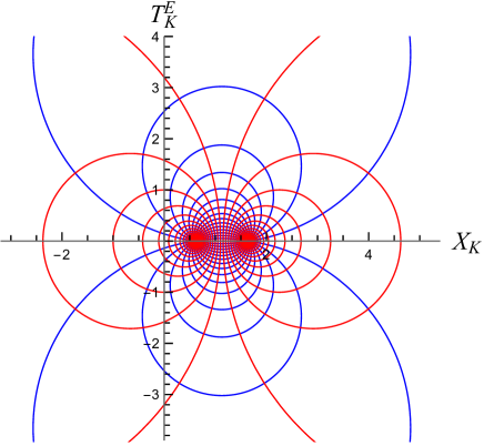
Figure 9: Euclidean $\text{dS}_{2}$ diamond spacetime in Kruskal coordinates $(T^{\text{E}}_{\text{K}},X_{\text{K}})$ (258). Lines of constant $x$ (red) and lines of constant $s_{\text{E}}$ (blue) are at equal intervals of 0.2. High contour density corresponds to the two horizon punctures at $x=\pm\infty$. We have set $a=b=1/2$, $L=\kappa_{a}=\kappa_{b}=1$ and $u_{0}\neq v_{0}\neq 0$. For the square diamond, the punctures at $x\to\pm\infty$ are mapped to the points $(T_{\text{K}}^{\text{E}},X_{\text{K}})=(0,Le^{\pm a/L})$.

The Euclidean continuation of the diamond universe coordinates follows from Wick rotating the conformal Killing time $s\to-is_{\text{E}}$. Similar to causal diamonds in four dimensions Banks:2020tox , the Euclidean continuation of the finite diamond covers nearly the entire space of Euclidean $\text{dS}_{2}$; only the bifurcation points $x\to\pm\infty$ are missing (see Appendix D). Thus, the null boundaries are mapped to punctures in the Euclidean spacetime, and correspond to a conical singularity $\varrho=0$ in the Rindler metric (143). To remove the conical singularity, we must periodically identify the Euclidean time coordinate, $s_{\text{E}}\sim s_{\text{E}}+2\pi/\kappa$. As such, when we restrict the Bunch–Davies state to the causal diamond, the diamond has a natural temperature $T_{\text{CD}}=\kappa/2\pi$. Thus, the Euclidean causal diamond in dS₂ may be represented by a two-sphere with two punctures corresponding to the horizons of the Lorentzian diamond. We illustrate the Euclidean diamond spacetime in Figure 9.

4.3 Generalized entropy from the microcanonical action

We now have all of the ingredients to find the microcanonical action of $\text{dS}_{2}$ causal diamonds in semi-classical JT gravity. We start from the microcanonical density of states $W(E_{0})$ (136) in the saddle point approximation, where $\psi_{0}=\{g_{\mu\nu},\phi,\chi\}$ are the solutions to the semi-classical JT equations. Following Pedraza:2021ssc , the off-shell Euclidean microcanonical action for causal diamonds is defined as

$$\begin{split}I^{\text{mc}}_{\text{E}}&\equiv-i\left[\int_{\mathcal{M}_{\text{E}}^{\text{CD}}}L-\int_{\mathcal{M}_{\text{E}}^{\text{CD}}}ds\wedge\theta(\psi,\mathcal{L}_{\zeta}\psi)\right].\end{split}$$ (144)

This differs from the microcanonical action for black holes (138), since causal diamonds have no asymptotic region like black holes and they admit a conformal isometry instead of a true isometry. Here $\theta$ is the symplectic potential 1-form, with $\theta(\psi,\mathcal{L}_{\zeta}\psi)$ non-vanishing since $\zeta$ is a conformal Killing vector rather than an exact Killing vector. Writing $L=ds\wedge\zeta\cdot L$, we see the two terms between brackets combine into an integral over the Noether current 1-form $j_{\zeta}\equiv\theta(\psi,\mathcal{L}_{\zeta}\psi)-\zeta\cdot L$ associated with diffeomorphisms generated by $\zeta$. Using the on-shell identity $j_{\zeta}=dQ_{\zeta}$, with $Q_{\zeta}$ the Noether charge 0-form, and applying Stokes’ theorem we find the on-shell Euclidean microcanonical action for diamonds is equal to

$$I^{\text{mc}}_{\text{E}}=\int_{\partial\mathcal{M}_{\text{E}}^{\text{CD}}}ds_{E}\wedge Q_{\zeta}=\frac{2\pi}{\kappa}\oint_{\partial\Sigma}Q_{\zeta}=-S_{\text{Wald}}\big{|}_{\partial\Sigma}\;.$$ (145)

To arrive to the second equality we used the fact that $\partial\mathcal{M}_{\text{E}}^{\text{CD}}$ has topology $S^{1}\times\partial\Sigma$, such that the Noether charge restricted to $\partial\Sigma$ is independent of Euclidean time $s_{E}$ since the dilaton $\phi$ and auxiliary field $\chi$ are constant in the limit $x\to\pm\infty.$ This allows us to integrate out the Euclidean time. The last equality follows from the definition of the Wald entropy, with $S_{\text{Wald}}=\frac{1}{4G_{2}}(\phi_{0}+\phi)-\frac{c}{6}\chi$. Thus, the on-shell microcanonical action of Euclidean $\text{dS}_{2}$ causal diamonds is equal to minus the Wald entropy.

Equivalently, the on-shell microcanonical action (145) is given by a GHY boundary term inserted at the bifurcation points $\{\partial\Sigma:x=\pm\infty\}$ Banks:2020tox ; Pedraza:2021ssc . To see this, note the Hamiltonian $H_{\zeta}$ for a theory, which fixes the induced metric of the boundary $\partial\mathcal{M}$ of a (Lorentzian) manifold $\mathcal{M}$, is given by an integral over the codimension-2 slices $\mathcal{C}_{s}$ where $\Sigma_{s}$ orthogonally intersects $\partial\mathcal{M}$ Pedraza:2021cvx ; Iyer:1995kg ,

$$H_{\zeta}=\oint_{\mathcal{C}_{s}}(Q_{\zeta}-\zeta\cdot b)=\oint_{\mathcal{C}_{s}}\epsilon_{\partial\Sigma}N\varepsilon\;.$$ (146)

Here $b$ is the GHY boundary term 1-form (217), $\varepsilon$ is the quasi-local energy density (231), and $N=-\zeta^{\mu}u_{\mu}$ is the lapse. Importantly, at the bifurcation points $\partial\Sigma$ the lapse $N=0$ such that $H_{\zeta}=0$ on $\partial\Sigma$. Now, let $(\partial\Sigma)_{\epsilon}$ denote a 1-parameter family of surfaces in $\Sigma_{s_{\text{E}}}$ obeying $\lim_{\epsilon\to 0}(\partial\Sigma)_{\epsilon}\to\partial\Sigma$. Using $H_{\zeta}=0$ in (146), it follows

$$\lim_{\epsilon\to 0}\int_{(\partial\Sigma)_{\epsilon}}Q_{\zeta}=\lim_{\epsilon\to 0}\int_{(\partial\Sigma)_{\epsilon}}\zeta\cdot b~{},$$ (147)

leading to, for the case of semi-classical JT gravity,

$$I^{\text{mc}}_{\text{E}}=-\lim_{\epsilon\to 0}\int_{\partial D_{\epsilon}\times\partial\Sigma}ds_{E}\sqrt{\gamma}K\left[\frac{(\phi_{0}+\phi)}{8\pi G_{2}}-\frac{c\chi}{12\pi}\right]\;.$$ (148)

Here $\sqrt{\gamma}=C$ is the induced metric on constant $s_{E}$ slices and the trace of the extrinsic curvature of these slices is $K=\mp C^{-2}\partial_{x}C$. Since the fields $\phi$, $\chi$ are independent of $s_{\text{E}}$ and $\sqrt{\gamma}K\to\kappa$ in the limit $x\to\pm\infty$, the integral over $s_{\text{E}}$ is trivial, and the right-hand side is equal to minus the Wald entropy. This establishes the equivalence between the BTZ Banados:1993qp ; Banks:2020tox and Noether charge Iyer:1995kg methods for the case of causal diamonds.

From either (145) or (148), since $S_{\text{Wald}}=S_{\text{gen}}$ (107), we see the on-shell microcanonical action in semi-classical JT gravity is given by the generalized entropy

$$I^{\text{mc}}_{\text{E}}=-S_{\text{gen}}\big{|}_{\partial\Sigma}\;.$$ (149)

The density of states is thus $W(E_{0})\approx e^{S_{\text{gen}}}$, identifying $S_{\text{gen}}$ as the microcanonical entropy. As a microcanonical entropy, $S_{\text{gen}}$ is maximized at a fixed energy. Therefore, the microcanonical action is minimized at fixed energy $E_{0}$. We may formally determine the energy $E_{0}$ by computing the variation of $I_{E}^{\text{mc}}$ over the full Euclidean causal diamond. Specifically,

$$\delta I_{\text{E}}^{\text{mc}}=\int_{\mathcal{M}_{\text{E}}^{\text{CD}}}ds_{\text{E}}\wedge\omega(\psi,\delta\psi,\mathcal{L}_{\zeta}\psi)=\int_{S^{1}}ds_{\text{E}}\delta H_{\zeta}\;,$$ (150)

where $\delta H_{\zeta}=\int_{\Sigma_{s_{\text{E}}}}\omega(\psi,\delta\psi,\mathcal{L}_{\zeta}\psi)$ is the variation of the Hamiltonian generating the evolution along $\zeta$. This shows $I_{\text{E}}^{\text{mc}}$ is stationary at fixed energy $E_{0}=\pm H_{\zeta}+\text{const}$. We set the constant to zero, and the sign is determined by imposing consistency with the first law of causal diamonds, $\frac{\kappa}{2\pi}\delta S_{\text{Wald}}=-\delta H_{\zeta}$ Jacobson:2018ahi ; Pedraza:2021ssc . Hence, the energy to be fixed is $E_{0}=-H_{\zeta}$.

Furthermore, minimizing the microcanonical action with respect to the background is equivalent to extremizing $S_{\text{gen}}$ with respect to the shape and location of $\partial\Sigma$. This is consistent with the extremization prescription in the QES formula. One subtle difference with the QES formula is that we derived the extremization of $S_{\text{gen}}$ in Euclidean signature, whereas the QES formula is usually stated in Lorentzian signature. We have thus derived the generalized entropy in de Sitter JT gravity and its extremization from a Euclidean action principle.

Lastly, note that here the Euclidean time $s_{\text{E}}=is$ is imposed to be periodic, $s_{\text{E}}\sim s_{\text{E}}+\frac{2\pi}{\kappa}$, in order to remove the conical singularities at $x=\pm\infty$. This is a regularity condition at the horizon which happens to be consistent with our choice of vacuum state. Thus, while we work in the microcanonical ensemble, the vacuum state of matter remains in the Bunch–Davies vacuum, which is a thermal state when restricted to the causal diamond at a fixed, positive temperature $T_{\text{CD}}=\kappa/2\pi$.

4.4 Islands in the full reduction

Quantum extremal surfaces arise from extremizing the generalized entropy (104), where the von Neumann entropy (106) is of a single interval with endpoints $[(U_{1},V_{1}),(U_{2},V_{2})]$. Equivalently, we search for QESs by minimizing the microcanonical action of a causal diamond in $\text{dS}_{2}$, where the bifurcation points $\partial\Sigma$ of the diamond are identified with the endpoints of the interval. In our computation, we will keep one endpoint of the interval fixed, and vary the position of the other endpoint. When looking for QESs, it is important to distinguish between the $\text{dS}_{2}$ geometry which arises from the half or full spherical reduction. In the full reduction, one may consider an interval with one endpoint in one hyperbolic patch, and another endpoint in a different hyperbolic patch. The authors of Hartman:2020khs showed non-pathological quantum extremal islands only arise in this scenario, thus implying islands do not arise in the half reduction model. Our calculations below are consistent with the results in Hartman:2020khs .

QESs in half reduction

Let us look for quantum extremal surfaces, and, consequently, islands, in the $\text{dS}_{2}$ geometry found via half reduction (Figure 2). This follows from extremizing the generalized entropy. The matter entanglement entropy is given by the von Neumann entropy of the conformal matter, $\chi$, in the Bunch–Davies vacuum restricted to an interval with both endpoints in the half reduction dS₂ space. One can consider a similar set-up for the $\text{dS}_{2}$ geometry from full reduction, and therefore our discussion here applies equally to that case as well (hence $\phi_{0}$ is not set to zero).

The total generalized entropy (104) is

$$S_{\text{gen}}=\frac{1}{4G}\left(\phi_{0}+\phi_{r}\left(\frac{1+\frac{U_{1}V_{1}}{L^{2}}}{1-\frac{U_{1}V_{1}}{L^{2}}}\right)+\frac{Gc}{3}\right)+\frac{c}{12}\log\left[\frac{16}{\delta_{1}^{2}\delta_{2}^{2}}\frac{(U_{2}-U_{1})^{2}(V_{2}-V_{1})^{2}}{\left(1-\frac{U_{1}V_{1}}{L^{2}}\right)^{2}\left(1-\frac{U_{2}V_{2}}{L^{2}}\right)^{2}}\right]\;.$$ (151)

Here we will keep the endpoint $(U_{2},V_{2})$ fixed while varying the first endpoint $(U_{1},V_{1})$. Doing so, we find two possible locations for a QES. The first is at

$$V_{1}\approx\frac{L^{2}\epsilon}{3U_{2}}+\mathcal{O}(\epsilon^{2})\;,\quad U_{1}\approx\frac{L^{2}\epsilon}{3V_{2}}+\mathcal{O}(\epsilon^{2})\;,$$ (152)

and the second is at

$$V_{1}\approx V_{2}-\frac{(L^{2}-2U_{2}V_{2})}{3U_{2}}\epsilon+\mathcal{O}(\epsilon^{2})\;,\quad U_{1}\approx U_{2}-\frac{(L^{2}-2U_{2}V_{2})}{3V_{2}}\epsilon+\mathcal{O}(\epsilon^{2})\;,$$ (153)

where $\epsilon\equiv\frac{G_{2}c}{\phi_{r}}\ll 1$. In the classical limit $\epsilon\to 0$, the first solution reduces to the cosmological horizon ($U_{1}=V_{1}=0$) for any choice of $(U_{2},V_{2})$. The second solution places the two endpoints very near each other, coinciding as $\epsilon\to 0$. We thus reject the second solution, and find that the QES (152) lies near the cosmological horizon,

$$r_{\text{QES}}\approx L-\frac{2L}{9}\left(\frac{L+r_{2}}{L-r_{2}}\right)\epsilon^{2}\;,$$ (154)

where $r_{2}$ denotes the radial coordinate associated with endpoint $(U_{2},V_{2})$. The location of this QES coincides with the one attained in Aalsma:2021bit . Further, note that for $U_{2}V_{2}=L^{2}$ or $r_{2}\to\infty$, then $S_{\text{gen}}(r=L)>S_{\text{gen}}(r=r_{\text{QES}})$, consistent with the QES formula. Further, the generalized entropy for the second solution (153) is parametrically larger than $S_{\text{gen}}$ evaluated at the QES in (152), which is another reason to ignore the second solution.

The island formula is an application of the QES formula (4), which may be used to compute the von Neumann entropy associated with radiation emitted from a horizon. Formally, one computes the von Neumann entropy associated to the entanglement wedge of radiation, namely, the causal development of the codimension-1 slice $\Sigma_{\partial I}=\Sigma_{\text{rad}}\cup I$. One imagines collecting the radiation in a weakly gravitating region $\Sigma_{\text{rad}}$, here placed near future infinity $\mathcal{I}^{+}$, as the dilaton diverges near there, a herald for weak gravity. The boundary of the island $\partial I$ corresponds to the location of the QES. For $\Sigma_{\text{rad}}$ near $\mathcal{I}^{+}$ ($r_{2}\to\infty$) we see the QES (154) is located just outside of the cosmological horizon, and hence the island is timelike separated from the radiation region $\Sigma_{\text{rad}}$. While computing the entanglement entropy of an interval between timelike separated points is not unreasonable, such entropies have been shown to lead to bag-of-gold and strong subadditivity paradoxes Anous:2020lka ; Chen:2020tes . Moreover, our derivation of the QES prescription only applies for an interval between spacelike separated points, and therefore, as in Hartman:2020khs , we neglect such scenarios. Consequently, there are no non-trivial islands spacelike separated from $\Sigma_{\text{rad}}$ to consider.

QESs in full reduction

We now turn to the $\text{dS}_{2}$ geometry found via full reduction, where we place the endpoint $(U_{1},V_{1})$ inside the hyperbolic patch coinciding with the black hole interior, whilst fixing the endpoint $(U_{2},V_{2})$ in the neighboring hyperbolic patch (future blue region in Figure 3). To move the point $(U_{1},V_{1})$ into the other hyperbolic patch we employ the continuation (195), such that the generalized entropy is now

$$S_{\text{gen}}=\frac{1}{4G}\left(\phi_{0}-\phi_{r}\left(\frac{1+\frac{U_{1}V_{1}}{L^{2}}}{1-\frac{U_{1}V_{1}}{L^{2}}}\right)+\frac{Gc}{3}\right)+\frac{c}{12}\log\left[\frac{16L^{4}}{\delta_{1}^{2}\delta_{2}^{2}}\frac{(L^{2}+U_{1}U_{2})^{2}(L^{2}+V_{1}V_{2})^{2}}{(L^{2}-U_{1}V_{1})^{2}(L^{2}-U_{2}V_{2})^{2}}\right]\;,$$ (155)

where we point out the relative minus sign in front of $\phi_{r}$ in the “area” term. It is worth noting that the quantum state of matter is in the vacuum with respect to global coordinates of the full space $(\sigma,\varphi)$ (184). This vacuum state is still the Bunch–Davies vacuum, which follows from the fact the continuation (195) leaves the line element invariant.

Figure 10: Islands in two-dimensional de Sitter in the full reduction. When an island $I$ is included, the entanglement wedge of radiation is the causal development of $\Sigma_{\text{rad}}\cup I$. Since the global vacuum state is pure, one instead computes the entanglement entropy of the complement $(\Sigma_{\text{rad}}\cup I)^{c}$, the two intervals $[Q_{L},P_{L}]\cup[P_{R},Q_{R}]$ (purple). The entanglement wedge of the complement is given by two rectangular causal diamonds (blue).

Varying with respect to endpoint $(U_{1},V_{1})$ while keeping $(U_{2},V_{2})$ fixed, we find two possible locations for a QES. The first one is

$$V_{1}\approx\frac{U_{2}\epsilon}{3}+\mathcal{O}(\epsilon^{2})\;,\quad U_{1}\approx\frac{V_{2}\epsilon}{3}+\mathcal{O}(\epsilon^{2})\;,$$ (156)

and the second is

$$V_{1}\approx-\frac{L^{2}}{V_{2}}+\left(\frac{2L^{2}}{3V_{2}}-\frac{U_{2}}{3}\right)\epsilon+\mathcal{O}(\epsilon^{2})\;,\quad U_{1}\approx-\frac{L^{2}}{U_{2}}+\left(\frac{2L^{2}}{3U_{2}}-\frac{V_{2}}{3}\right)\epsilon+\mathcal{O}(\epsilon^{2})\;.$$ (157)

When the point $(U_{2},V_{2})$ lives near $\mathcal{I}^{+}$, it is straightforward to show the second solution (157) is timelike separated from the radiation region, and for the reasons described above, we neglect such a solution. The first solution (156) is located near the black hole singularity, and thus the associated island is spacelike separated from $\Sigma_{\text{rad}}$ (see Figure 10). In static patch coordinates, the QES (156) is

$$r_{\text{QES}}\approx-L+\frac{2L}{9}\left(\frac{L-r_{2}}{L+r_{2}}\right)\epsilon^{2}\;.$$ (158)

This QES is the same one uncovered in Hartman:2020khs . In the classical limit, the QES lies at the black hole horizon $r=-L$, while for $\epsilon\neq 0$ and $r_{2}\to\infty$, the value of the dilaton at this QES is

$$\phi(r_{\text{QES}})=-\frac{\phi_{r}}{L}r_{\text{QES}}+\frac{Gc}{3}=-\phi_{r}\sqrt{1+\left(\frac{2\epsilon}{3}\right)^{2}}+\frac{Gc}{3}\;.$$ (159)

As in the half reduction model, $S_{\text{gen}}(r=r_{\text{QES}})<S_{\text{gen}}(r=-L)$, consistent with the QES formula.

Figure 11: Causal diamond associated with computing semi-classical entanglement entropy of $\Sigma_{\text{rad}}$ in the absence of an island.

Note that the radiation, modeled by $\chi$, is in the Bunch–Davies vacuum, a pure state. Hence, $S_{\text{vN}}(\Sigma_{\partial I})=S_{\text{vN}}(\Sigma_{\partial I}^{c})$, where $\Sigma_{\partial I}^{c}=(\Sigma_{\text{rad}}\cup I)^{c}$ is the complement of $\Sigma_{\partial I}=\Sigma_{\text{rad}}\cup I$, and in practice we therefore compute $S_{\text{vN}}(\Sigma_{\partial I}^{c})$ using the island formula. Thus we consider the microcanonical action of the complement of the entanglement wedge of radiation: the union of the domain of dependence of achronal surfaces $\Sigma$ and $\Sigma^{\prime}$ with boundaries $\partial\Sigma=\mathcal{B}\cup P_{L}$ and $\partial\Sigma^{\prime}=P_{R}\cup\mathcal{B}^{\prime}$, respectively. Upon extremizing the microcanonical action, the point $\mathcal{B}$ becomes the QES $Q_{L}$, and similarly $\mathcal{B}^{\prime}=Q_{R}$, such that we compute the entropy of the two intervals $[Q_{L},P_{L}]\cup[P_{R},Q_{R}]$, and the island is $I=[Q_{L},Q_{R}]$ with boundary $\partial I=Q_{R}\cup Q_{L}$ (Figure 10). We thus evaluate the on-shell microcanonical action for two identical causal diamonds with edges $\partial\Sigma$ and $\partial\Sigma^{\prime}$. In the previous subsection we showed the on-shell (Euclidean) microcanonical action of a causal diamond in semiclassical JT gravity is equal to minus the generalized entropy of the diamond. Even though the causal diamonds in Figure 10 include the black hole singularity, this does not pose a problem to evaluating the microcanonical action of the diamonds. The action is on-shell given by a boundary term, i.e. ($\beta$ times) the Noether charge of the edge $\partial\Sigma$, which is not close to the black hole singularity.

In an appropriate OPE limit, the von Neumann entropy of the CFT factorizes, such that we may treat each causal diamond separately. Consequently, the total island entropy is, to leading order in $U_{2}V_{2}\approx L^{2}$,

$$S_{\text{vN}}(\Sigma_{\partial I}) =S_{\text{gen}}(Q_{L})+S_{\text{gen}}(Q_{R})$$ (160)

$$\approx\frac{2}{4G}\left(\phi_{0}+\phi(r_{\text{QES}})\right)+\frac{c}{3}\log\left[\frac{4L^{4}}{\delta_{1}\delta_{2}(L^{2}-U_{2}V_{2})}\right]+\frac{2c\epsilon}{9}\;,$$

consistent with the result found in Hartman:2020khs . Here we used $S_{\text{gen}}|_{\partial\Sigma}=S_{\text{gen}}(Q_{L})$, and similarly for $S_{\text{gen}}|_{\partial\Sigma^{\prime}}$, since $P_{R,L}$ belong to the weakly gravitating region, such that we ignore the contribution to the dilaton, and where $\chi=0$, due to the Dirichlet boundary condition imposed on $\chi$ (see footnote 10) Pedraza:2021cvx .

Note that the entropy (160) is constant with respect to time $t$ or equivalently “length” $X=\frac{L}{2}\log(V/U)$ in coordinates (191). This is analogous to the behavior of the entropy of radiation emitted by an eternal $\text{AdS}_{2}$ black hole in the island phase Almheiri:2019yqk . When the island is taken to be the empty set, however, one neglects the dilaton and the von Neumann entropy of radiation is given by the semi-classical entanglement entropy, which is found to grow linearly in $X$ at large $X$ Hartman:2020khs . The linear growth also follows from extremizing the microcanonical action, where now there is only a single (square) causal diamond with edges $\partial\Sigma=P_{L}\cup P_{R}$ (Figure 11). Specifically, similar to Pedraza:2021ssc , extremization of $S_{\text{vN}}^{\text{sc}}$ for a single interval contained in the expanding hyperbolic patch yields $U_{L}=V_{R}$ and $V_{L}=U_{R}$ (such that $T_{R}=T_{L}\equiv T$ and $X_{R}=-X_{L}\equiv X$), and $X\gg L$ and $T\ll L$. Substituting these conditions into the semi-classical entanglement entropy gives

$$S_{\text{vN}}^{\text{sc}}(\Sigma_{\text{rad}})=\frac{c}{3}\log\left(\frac{2L^{2}(V_{R}-U_{R})}{\delta(L^{2}-U_{R}V_{R})}\right)=\frac{c}{3}\log\left(\frac{2L}{\delta}\frac{\sinh X}{\sinh(-T)}\right)\approx\frac{c}{3}\frac{X}{L}+...\;,$$ (161)

where we expanded for $X\gg L$ to obtain the linear growth in $X$, analogous to the “Hawking phase” for black hole radiation, and in agreement with Hartman:2020khs . There exists a critical length, the “Page length” $X_{\text{P}}$ at which the island entropy (160) equals the semi-classical entanglement entropy (161):

$$(V_{P}-U_{P})\approx\frac{2L^{2}}{\delta_{1}}e^{\frac{6}{4Gc}[\phi_{0}+\phi(r_{\text{QES}})]}\;,\;\;\text{or}\;\;\;X_{\text{P}}\approx L\text{arcsinh}\left(\frac{L}{\delta_{1}}e^{\frac{6}{4Gc}[\phi_{0}+\phi(r_{\text{QES}})]}\right)\;.$$ (162)

A global minimization of entropies (161) and (160) reveals a transition occurring at this length, analogous to the transition seen in the Page curve for eternal $\text{AdS}_{2}$ black holes Almheiri:2019yqk .

5 Discussion

In this article we explored thermodynamic and microscopic aspects of two-dimensional de Sitter space using semi-classical de Sitter JT gravity. Specifically, we extended the quasi-local analysis of York to the case of $\text{dS}_{2}$ by introducing an auxiliary timelike boundary in the static patch that interpolates between the black hole and cosmological horizons. With this timelike boundary we were able to properly define conserved charges, namely the energy, and uncovered a quasi-local first law of thermodynamics. Backreaction due to quantum matter is fully incorporated via the 1-loop Polyakov action, leading to a semi-classical extension of the quasi-local first law of thermodynamics, where the classical Gibbons–Hawking entropy is replaced by the generalized entropy. Crucial to this extension was the observation that in two dimensions the semi-classical Wald entropy is exactly equal to the generalized entropy, where the semi-classical contribution arises from expressing the Polyakov action in a localized form. Including semi-classical backreaction, the first law of horizon thermodynamics was modified such that the classical entropy is replaced by the generalized entropy. This is expected to be a feature for systems which include backreaction; indeed, the same modification appears in the three-dimensional semi-classical Schwarzschild-de Sitter black hole Emparan:2022ijy .

Further, in the microcanonical ensemble, we found that the generalized entropy is equal to the microcanonical entropy, whose stationarity condition implies extremizing the generalized entropy, similar to recent results for eternal $\text{AdS}_{2}$ black holes Pedraza:2021cvx . This observation suggests a first principles derivation of the QES formula Pedraza:2021ssc in $U(1)$ symmetric backgrounds (alternative to previous derivations invoking the replica trick) which we have extended to the case of de Sitter JT gravity. Thus, we provided evidence that the QES and island prescriptions hold beyond $\text{AdS}_{2}$ systems. The crucial new insight is that the on-shell microcanonical action of (Euclidean) causal diamonds computes the generalized entropy, whose extremization follows from the minimization of the action. This leads to the appearance of quantum extremal islands in the full reduction model of JT gravity, consistent with Hartman:2020khs , where the island lives near the singularity of the black hole.

There are a number of exciting prospects of our work, which we have only eluded to thus far. Let us discuss them now in some detail.

De Sitter holography.

The Gibbons–Hawking entropy formula suggests the microscopic description of de Sitter space obeys the holographic principle. That is, the putative dual quantum theory accounting for the underlying microscopics of dS lives on a holographic screen. Evidence is mounting that dS holography is strikingly different from AdS/CFT holography (cf. Leuven:2018ejp ). For example, the number of degrees of freedom increases in the IR direction of the microscopic theory, indicating the dual quantum theory description of dS is unlikely to be a local quantum field theory. Additional evidence that the underlying microscopics of de Sitter space is not well characterized by a local quantum field theory has been given via matrix model descriptions of $\text{dS}_{2}$ Anninos:2021eit . Further, the UV/IR connection for dS appears to be inverted: long distances (IR) in the bulk correspond to low energies (IR) in the microscopic theory. This is consistent with the worldline holography proposed in Anninos:2011af (see also Anninos:2017hhn ) where the UV theory lives on a surface near the origin $r=0$, in contrast with AdS/CFT where the UV description lies on the conformal boundary.

The differences between dS holography and AdS/CFT are further exemplified in the way entanglement entropy of the dual quantum mechanical theory is computed using bulk quantities. The Ryu–Takayanagi entropy formula says that the entanglement entropy of a CFT state restricted to a boundary subregion is equal to the area of the (bulk AdS) extremal surface anchored at the endpoints of the boundary subregion. In contrast, it was recently proposed that in de Sitter space the extremal surface whose area computes the entanglement entropy is anchored between the two stretched horizons where the holographic degrees of freedom reside Susskind:2021dfc ; Susskind:2021esx ; Shaghoulian:2021cef ; Shaghoulian:2022fop (see also Sanches:2016sxy ; Nomura:2017fyh ). Thus, the UV boundary of AdS is replaced by the IR boundary of the static patch, compatible with the aforementioned worldline holography.

A toy quantum mechanical model which exhibits these features of static patch holography has been conjectured to be the SYK model in the “hyperfast” limit Susskind:2021esx . This is because the holographic degrees of freedom of the cosmological horizon are hyperfast scramblers, scrambling on a time scale equal to the de Sitter radius, implying the complexity growth is hyperfast. In the SYK model, the hyperfast scrambling property is a consequence of taking the infinite temperature limit of SYK, such that the temperature is greater or equal to the fundamental energy scale of SYK.

The transition from low to high temperature in the dual bulk (AdS JT gravity) picture suggests a connection with the quasi-local thermodynamics studied here. At low temperature, the boundary bends slightly inward toward the horizon Maldacena:2016upp , while at high temperature the boundary nearly coincides with the horizon, such that the holographic boundary degrees of freedom become horizon quasinormal modes. The timelike screen one introduces to study quasi-local thermodynamics interpolates between the UV $(r=0)$ surface and the IR static patch boundary (strechted horizon), and shifting its position may be capturing this low to high temperature transition of SYK. It would be interesting to pursue this connection further and see whether the quasi-local thermodynamics of dS JT gravity provides insights into hyperfast SYK, and vice versa.

Furthermore, the semi-classical thermodynamics may deepen our understanding of entanglement entropy in de Sitter space. For example, according to the proposals of Susskind:2021dfc ; Shaghoulian:2021cef ; Shaghoulian:2022fop , the Gibbons–Hawking entropy of pure dS is identified with the entanglement entropy between modes living on the left and right horizons, $S_{\text{ent}}=S_{\text{GH}}$. Similarly, the entanglement entropy between left and right sides in a Schwarzschild-de Sitter background is given by the sum of the gravitational entropies of the black hole and cosmological horizon, $S_{\text{ent}}=S_{\text{h}}+S_{\text{c}}$. Therefore, thermodynamic relations directly translate into relations for the entanglement entropy. Our global first law for dS₂ (125) suggests that when quantum matter is included, the total semi-classical entropy of SdS is $S_{\text{ent}}=S_{\text{gen,h}}+S_{\text{gen,c}}$. Moreover, semi-classical corrections affect the probability of creating a black hole in de Sitter, which in semi-classical gravity should be $P\sim\exp(-\Delta S)$ with entropy deficit $\Delta S=S_{\text{gen,dS}}-S_{\text{gen,h}}-S_{\text{gen,c}}$, where the last term is the generalized entropy of pure dS. This semi-classical modification of the entropy deficit also features in the three-dimensional semi-classical Schwarzschild-de Sitter black hole Emparan:2022ijy .

Quasi-local thermodynamics and $T\bar{T}$ deformations in $\text{dS}_{2}$.

It is well known that finite cutoff holography in $\text{AdS}_{3}$ is dual to $T\bar{T}$ deformations of a holographic CFT, where $T\bar{T}$ is related to the trace of the quasi-local Brown-York stress tensor. Further, AdS JT gravity with a finite cutoff is precisely described by a Schwarzian theory deformed by the one-dimensonal analog of $T\bar{T}$ Iliesiu:2020zld , providing evidence that $T\bar{T}$ deformations in a holographic theory correspond to moving the conformal boundary to a finite radial distance in bulk AdS. In three (bulk) dimensions, these deformations were generalized to $T\bar{T}+\Lambda_{2}$ deformations of the CFT to reconstruct patches in three-dimensional de Sitter space Gorbenko:2018oov , and were recently used to provide a microstate counting interpretation of the Gibbons–Hawking entropy of global de Sitter space Coleman:2021nor . In particular, one constructs microstates of the patch containing the cosmological horizon from the (dressed) microstates of the BTZ black hole at a particular energy level. This “cosmic horizon patch” is defined as the region between the cosmological horizon and a timelike boundary $B$. This picture suggests, holographically, that the $T\bar{T}$ deformation corresponds to the movement of a holographic screen in the bulk. The quasi-local thermodynamics studied here may shed light on the one-dimensional analog of $T\bar{T}$ deformations to the dual quantum mechanical theory.

Microcanonical action and multiverse models.

We found that the von Neumann entropy of radiation collected at $\mathcal{I}^{+}$ in global $\text{dS}_{2}$ during the island phase is equivalent to evaluating the microcanonical action on two finite causal diamonds (Figure 10). Recently, JT de Sitter multiverses, where global $\text{dS}_{2}$ is extended, have been used as toy models to study false vacuum decay in inflationary universes with multiple vacua. For sufficiently large radiation subregions $\Sigma_{\text{rad}}$, the fine grained entropy of radiation, captured using the island rule, leads to an analogous Page-like transition Aguilar-Gutierrez:2021bns . Crucial to this analysis is the assumption the island formula holds for the extended $\text{dS}_{2}$ multiverse. However, it is not immediately clear how reasonable this assumption is as a Euclidean description of JT multiverses is currently lacking, as is the replicated manifold necessary for the replica trick.

An appealing feature of our first principles derivation of the QES prescription is that it naturally applies to these multiverse models. We find an island develops and covers nearly the entire $\text{dS}_{2}$ multiverse, consistent with Aguilar-Gutierrez:2021bns . To carry out the analysis explicitly, one must consider causal diamonds in extended $\text{dS}_{2}^{n}$, which globally has the same line element and static dilaton solution as in (185), except where the coordinate $\varphi\in(0,2\pi n)$ for integer $n$. The Euclidean diamond universe in $\text{dS}_{2}^{n}$, which the microcanonical action is evaluated over, is given by the Euclidean continuation of $\text{dS}_{2}^{n}$, modulo the horizon bifurcation points. The calculation then proceeds as before (148), where the microcanonical action is equal to the Gibbons–Hawking–York boundary term evaluated on the boundary of an infinitesimal disk surrounding the punctures. This is reminiscent of the observation made in Aguilar-Gutierrez:2021bns : an island always forms for sufficiently large $\Sigma_{\text{rad}}$, independent of the global geometry beyond $\Sigma_{\text{rad}}$. This suggests the global spacetime does not capture fundamental degrees of freedom independent from those in $\Sigma_{\text{rad}}$, i.e., there is a redundancy in the rest of the global spacetime.

Dynamical backgrounds and beyond two dimensions.

Our derivation of the QES prescription only applies to two-dimensional static backgrounds. It is natural to wonder whether we can extend this work to higher-dimensional and dynamical settings. The derivation $I_{\text{E}}^{\text{mc}}=-S_{\text{Wald}}$ for causal diamonds is actually valid for any diffeomorphism invariant theory in any dimension Pedraza:2021ssc . It is unclear, however, whether the connection $S_{\text{Wald}}=S_{\text{gen}}$ holds beyond two dimensions; in fact it seems unlikely since here we used the fact that the Polyakov action is 1-loop exact in two dimensions. Nonetheless, it would be interesting to see what one could glean from the Wald entropy associated with the anomaly induced action for four-dimensional general relativity. Finally, our results reasonably apply in equilibrium settings, and therefore we cannot comment on Page curves in dynamical backgrounds, including the $\text{dS}_{2}$ scenarios described in Sybesma:2020fxg ; Aalsma:2021bit ; Kames-King:2021etp ; Teresi:2021qff . It would be interesting to see whether one can express the dynamical black hole entropy proposal of Iyer:1994ys as a “microcanonical” action, and apply it to diamonds. This could also prove useful to extend the de Sitter holographic entropy proposals in Susskind:2021dfc ; Susskind:2021esx ; Shaghoulian:2021cef ; Shaghoulian:2022fop to dynamical setups. We leave this for future exploration.

Appendix A Reductions and coordinate systems

Here we provide details of the half and full spherical reductions of the $d$-dimensional Einstein–Hilbert action (5), leading to two different models of de Sitter JT gravity.

Half reduction

For the half reduction, consider the metric ansatz

$$d\ell^{2}=\hat{g}_{MN}dX^{M}dX^{N}=g_{\mu\nu}(x)dx^{\mu}dx^{\nu}+L^{2}_{d}\Phi^{2/(d-2)}(x)d\Omega_{d-2}^{2}\;.$$ (163)

Here $M,N=0,1,...,d-1$, $\mu,\nu=0,1$, and $\Phi(x)$ is the dilaton. A standard calculation using Cartan’s structure equations (see e.g. Grumiller:2001ea ; Narayan:2020pyj ) shows the $d$-dimensional Ricci scalar is

$$\hat{R}=R+\frac{(d-3)(d-2)}{L^{2}_{d}\Phi^{2/(d-2)}}+\frac{(d-3)}{(d-2)}\frac{1}{\Phi^{2}}(\nabla\Phi)^{2}-\frac{2}{\Phi}\Box\Phi\;,$$ (164)

where $R$ is the Ricci scalar and $\nabla$ the covariant derivative with respect to the two-dimensional metric $g_{\mu\nu}$. It is also straightforward to show the $(d-1)$-dimensional extrinsic curvature $\hat{K}$ reduces to

$$\hat{K}=K+\frac{1}{\Phi}n^{\mu}\nabla_{\mu}\Phi\;,$$ (165)

where $K$ is the extrinsic curvature of the 1-dimensional boundary and $n^{\mu}$ is the normal vector used to define the $(d-1)$-dimensional boundary metric. We further have

$$\int_{\hat{M}}d^{d}X\sqrt{-\hat{g}}=L_{d}^{(d-2)}\Omega_{d-2}\int_{\mathcal{M}}d^{2}x\sqrt{-g}\,\Phi\;,$$ (166)

where $\mathcal{M}$ is the two-dimensional Lorentzian manifold endowed with metric $g_{\mu\nu}$. Substituting the dimensionally reduced scalar curvatures (164) and (165), and (166) into the $d$-dimensional Einstein–Hilbert action results in the following two-dimensional dilaton theory of gravity,

$$\begin{split}I_{d}&=\frac{1}{16\pi G_{2}}\int_{\mathcal{M}}d^{2}x\sqrt{-g}\biggr{(}\Phi R-2\Lambda\Phi+\frac{(d-3)(d-2)}{L^{2}_{d}}\Phi^{\frac{(d-4)}{(d-2)}}+\frac{(d-3)}{(d-2)}\frac{(\nabla\Phi)^{2}}{\Phi}\biggr{)}\\ &+\frac{1}{8\pi G_{2}}\int_{\partial\mathcal{M}}dy\sqrt{-h}\Phi K\;,\end{split}$$ (167)

where we performed an integration by parts on the $\Box\Phi$ term in the two-dimensional “bulk” integral, which cancels against an identical term in the GHY integral, and we defined the two-dimensional Newton’s constant as

$$\frac{1}{G_{2}}\equiv\frac{L_{d}^{(d-2)}\Omega_{d-2}}{G_{d}}\,.$$ (168)

We notice a dramatic simplification when $d=3$:

$$I_{\text{JT}}=\frac{1}{16\pi G_{2}}\int_{\mathcal{M}}d^{2}x\sqrt{-g}\,\Phi\!\left(R-\frac{2}{L_{3}^{2}}\right)+\frac{1}{8\pi G_{2}}\int_{\partial\mathcal{M}}dy\sqrt{-h}\Phi K\;,$$ (169)

where $1/G_{2}=2\pi L_{3}/G_{3}$. Importantly, here the dilaton $\Phi$ only takes on positive values.

Full reduction

When $d=3$ the dimensionally reduced action (167) greatly simplifies since the potential and kinetic terms drop out. For $d>3$ this is no longer the case. For $d>3$ we can remove the kinetic term via an appropriate Weyl rescaling of the two-dimensional metric, such that a spherical reduction of the near-Nariai solution in $d$-dimensions leads to another form of de Sitter JT gravity. First, recall how the Ricci scalar and trace of the extrinsic curvature transform under the Weyl rescaling $\bar{g}_{\mu\nu}=\omega^{2}g_{\mu\nu}$ in a two-dimensional spacetime

$$\tilde{R}=\omega^{-2}R-2\omega^{-3}\Box\omega+2\omega^{-4}(\nabla\omega)^{2}\;,\quad\tilde{K}=\omega^{-1}K+\omega^{-2}n_{\mu}\nabla^{\mu}\omega\;.$$ (170)

Then, rescaling $g_{\mu\nu}\to\omega^{2}g_{\mu\nu}$, the reduced action (167) becomes

$$I_{d} =\frac{L_{d}^{(d-2)}\Omega_{d-2}}{16\pi G_{d}}\int_{\mathcal{M}}d^{2}x\sqrt{-g}\biggr{[}\Phi R-2\omega^{-1}\Phi\Box\omega+2\omega^{-2}\Phi(\nabla\omega)^{2}+\frac{(d-3)(d-2)\omega^{2}}{L_{d}^{2}}\Phi^{\frac{(d-4)}{(d-2)}}$$ (171)

$$-2\Lambda\Phi\omega^{2}+\frac{(d-3)}{(d-2)}\frac{1}{\Phi}(\nabla\Phi)^{2}\biggr{]}+\frac{L_{d}^{(d-2)}\Omega_{d-2}}{8\pi G_{d}}\int_{\partial\mathcal{M}}dy\sqrt{-h}(\Phi K+\omega^{-1}\Phi n_{\mu}\nabla^{\mu}\omega)\;.$$

By an integration by parts, the $\Box\omega$ term is partially cancelled by the GHY integral and after simplifying we are left with

$$\begin{split}I_{d}&=\frac{L_{d}^{(d-2)}\Omega_{d-2}}{16\pi G_{d}}\int d^{2}x\sqrt{-g}\biggr{[}\Phi R+2\omega^{-1}(\nabla^{\mu}\Phi)(\nabla_{\mu}\omega)+\frac{(d-3)}{(d-2)}\frac{1}{\Phi}(\nabla\Phi)^{2}-2\Lambda\Phi\omega^{2}\\ &+\frac{(d-3)(d-2)\omega^{2}}{L_{d}^{2}}\Phi^{\frac{(d-4)}{(d-2)}}\biggr{]}+\frac{\Omega_{d-2}}{8\pi G_{d}}\int_{\partial\mathcal{M}}dy\sqrt{-h}\Phi K\;.\end{split}$$ (172)

We can eliminate the kinetic term by choosing $\omega=\alpha\Phi^{\beta}$ for $\beta=-(d-3)/2(d-2)$ and $\alpha$ some constant, which we judiciously choose to be $\alpha=1/\sqrt{d-1}$. Then we have

$$I_{d}=\frac{L_{d}^{(d-2)}\Omega_{d-2}}{16\pi G_{d}}\int_{\mathcal{M}}d^{2}x\sqrt{-g}[\Phi R+U(\Phi)]+\frac{L_{d}^{(d-2)}\Omega_{d-2}}{8\pi G_{d}}\int_{\partial\mathcal{M}}dy\sqrt{-h}\Phi K\;,$$ (173)

where we have introduced the dilaton potential

$$U(\Phi)=\frac{(d-2)}{L_{d}^{2}}\left(\Phi^{-1/(d-2)}-\Phi^{1/(d-2)}\right)\;.$$ (174)

Let us now show how to derive the JT action from the Nariai limit of a $\text{SdS}_{d}$ black hole. This is accomplished by modifying the metric Ansatz (163) to

$$d\ell^{2}=\hat{g}_{MN}dX^{M}dX^{N}=g_{\mu\nu}(x)dx^{\mu}dx^{\nu}+r_{\text{N}}^{2}\Phi^{2/(d-2)}(x)d\Omega_{d-2}^{2}\;,$$ (175)

which reduces to the Nariai geometry (23) for $\Phi=1$. Moreover, clearly

$$U(\Phi=1)=0\;,\quad\frac{dU}{d\Phi}\biggr{|}_{\Phi=1}=-\frac{2}{L_{d}^{2}}\;.$$ (176)

Then, expanding the reduced action (173) about $\Phi\approx\phi_{0}+\phi$ for $\phi_{0}=1$, we find to leading order

$$\begin{split}I_{\text{JT}}&=\frac{1}{16\pi G_{2}}\int_{\mathcal{M}}d^{2}x\sqrt{-g}\left((\phi_{0}+\phi)R-\frac{2}{L_{d}^{2}}\phi\right)+\frac{1}{8\pi G_{2}}\int_{\partial\mathcal{M}}dy\sqrt{-h}(\phi_{0}+\phi)K\,,\end{split}$$ (177)

where we have identified the dimensionless two-dimensional Newton’s constant $G_{2}$ as

$$\frac{1}{G_{2}}\equiv\frac{\Omega_{d-2}r_{\text{N}}^{d-2}}{G_{d}}\;.$$ (178)

Notice then $\phi_{0}$ is proportional to the entropy (25) of the Nariai black hole:

$$\frac{\phi_{0}}{4G_{2}}=\frac{\Omega_{d-2}r_{\text{N}}^{d-2}}{4G_{d}}=\frac{1}{2}S_{\text{N}}\;.$$ (179)

Thus, analogous to the case of JT gravity in AdS, $\phi$ represents a deviation from the Nariai (“extremal”) solution.

Coordinate systems

Here we summarize various useful coordinates to describe two-dimensional de Sitter space (see also Maldacena:2019cbz ; Kames-King:2021etp ; Moitra:2022glw ).

Static patch.

In static patch coordinates $(t,r)$, the $\text{dS}_{2}$ line element and static dilaton take the form:

$$d\ell^{2}=-\left(1-\frac{r^{2}}{L^{2}}\right)dt^{2}+\left(1-\frac{r^{2}}{L^{2}}\right)^{-1}dr^{2}\;,\quad\phi(r)=\phi_{r}\frac{r}{L}\;.$$ (180)

Let $(v,u)$ denote advanced and retarded null coordinates for the static patch (180), respectively defined by

$$v=t+r_{\ast}\;,\quad u=t-r_{\ast}\;,$$ (181)

with $r_{\ast}$ being the tortoise coordinate,

$$r_{\ast}\equiv\int^{r}_{0}\frac{dr^{\prime}}{1-\frac{r^{\prime 2}}{L^{2}}}=L\text{arctanh}(r/L)\;.$$ (182)

In the full reduction the ranges are $r\in[-L,L]$ and $r_{\ast}\in[-\infty,\infty]$ in the static patch, where $r_{\ast}=\infty$ $(r=L)$ is the location of the cosmological horizon and $r_{\ast}=-\infty$ $(r=-L)$ is the location of the black hole horizon. In the half reduction the ranges are $r\in[0,L]$ and $r_{\ast}\in[0,\infty]$, where $r_{\ast}=\infty$ and $r=L$ correspond to the location of the cosmological horizon.

In these null coordinates the static patch line element (180) and dilaton become

$$d\ell^{2}=-\text{sech}^{2}\left(\frac{v-u}{2L}\right)dvdu\,,\;\quad\phi(u,v)=\phi_{r}\tanh\left(\frac{v-u}{2L}\right)\;.$$ (183)

Global conformal coordinates.

The full space of $\text{dS}_{2}$ is covered by global conformal coordinates $(\sigma,\varphi)$,

$$\tan\varphi=\frac{1}{r}\sqrt{L^{2}-r^{2}}\cosh(t/L)\;,\quad\tan\sigma=\frac{1}{L}\sqrt{L^{2}-r^{2}}\sinh(t/L)\;,$$ (184)

with line element and dilaton:

$$d\ell^{2}=\frac{L^{2}}{\cos^{2}\sigma}(-d\sigma^{2}+d\varphi^{2})\;,\quad\phi(\sigma,\varphi)=\phi_{r}\frac{\cos\varphi}{\cos\sigma}\;.$$ (185)

Here the ranges are $\sigma\in(-\pi/2,\pi/2)$, where future/past infinity corresponds to $\sigma=\pm\pi/2$, and $\varphi\in(0,2\pi)$ for the full reduction model. In the half reduction model the metric takes the same form, however, the dilaton is given by $\phi=\phi_{r}\frac{\sin\varphi}{\cos\sigma}$, with $\varphi\in(0,\pi)$.

Global coordinates.

In standard global coordinates the line element and dilaton are

$$d\ell^{2}=-d\tau^{2}+L^{2}\cosh^{2}(\tau/L)d\varphi^{2}\,,\qquad\phi(\tau,\varphi)=\phi_{r}\cos\varphi\cosh(\tau/L)\,,$$ (186)

where $\tau\in(-\infty,\infty)$ and the range of $\varphi$ is the same as for the global conformal coordinates. The global coordinates $(\tau,\varphi)$ are related to the static patch coordinates ($t,r$) by

$$r=L\cosh(\tau/L)\sin\varphi\,,\qquad\sinh(t/L)=\frac{\sinh(\tau/L)}{\sqrt{1-\cosh^{2}(\tau/L)\sin^{2}\varphi}}\,,$$ (187)

and to global conformal coordinates $(\sigma,\varphi)$ by

$$\tan(\sigma/2)=\tanh(\tau/2L)\,.$$ (188)

Kruskal coordinates.

We introduce global Kruskal-like coordinates $(V,U)$ to cover the full two-dimensional geometry in the half reduction model

$$V=Le^{v/L}=Le^{t/L}\sqrt{\frac{L-r}{L+r}}\;,\quad U=-Le^{-u/L}=-Le^{-t/L}\sqrt{\frac{L-r}{L+r}}\;.$$ (189)

The line element and dilaton become

$$d\ell^{2}=-\frac{4L^{4}}{\left(L^{2}-UV\right)^{2}}dVdU\;,\quad\phi(U,V)=\phi_{r}\left(\frac{L^{2}+UV}{L^{2}-UV}\right)\;.$$ (190)

In these coordinates, $UV=-L^{2}$ corresponds to the location of the poles $r=0$, while $UV=+L^{2}$ corresponds to the past and future conformal boundary $\mathcal{I}^{\pm}$. Moreover, the past (future) cosmological horizon is located at $V=0$ ($U=0$).

It is also useful to express Kruskal coordinates $(V,U)$ as

$$V=Le^{(T+X)/L}\;,\quad U=Le^{(T-X)/L}\;,$$ (191)

such that the line element (190) and static dilaton solution are

$$d\ell^{2}=\frac{1}{\sinh^{2}(T/L)}[-dT^{2}+dX^{2}]\;,\quad\phi(T)=-\phi_{r}\coth(T/L)\;.$$ (192)

In these coordinates $\mathcal{I}^{\pm}$ is located at $T=0$. The region to the future of the cosmological horizon is defined by $X\in\mathbb{R}$ and $T<0$, such that for $\phi_{r}>0$ the dilaton is strictly positive, diverging to $+\infty$ near $\mathcal{I}^{+}$. Coordinates $(T,X)$ are related to coordinates $(\sigma,\varphi)$ (184)

$$\sigma=L\arctan\left[-\frac{\cosh(X/L)}{\sinh(T/L)}\right]\;,\quad\varphi=L\arctan\left[\frac{\sinh(X/L)}{\cosh(T/L)}\right]\;,$$ (193)

and to static coordinates by

$$\coth(T/L)=-\frac{r}{L}\;,\quad\tanh(X/L)=\coth(t/L)\;.$$ (194)

Interior region in full reduction.

To describe physics in the interior region containing the black hole singularity in the full reduction model, one must analytically extend the Kruskal coordinates to move between each hyperbolic patch Hartman:2020khs . The standard branch of the $\arctan$ function in (193) only covers the hyperbolic region in the exterior of the black hole (blue region in Figure 3). The hyperbolic patch in the interior of the black hole (white region in Figure 3) is attained by shifting $\varphi/L\to\varphi/L+\pi$. This amounts to performing the continuation $(T,X)\to(-T+i\pi L,-X)$, such that

$$V\to-Le^{-(T+X)/L}=-\frac{L^{2}}{V}\;,\quad U\to-Le^{-(T-X)/L}=-\frac{L^{2}}{U}\;,$$ (195)

which leaves the line elements (190) and (192) invariant, but alters the sign of the dilaton, i.e., $\phi=-\phi_{r}\frac{L^{2}+UV}{L^{2}-UV}=\phi_{r}\coth(T/L)$. Equivalently, the continuation of static patch coordinates is $(t,r)\to(-t+i\pi L,-r)$, or $(v,u)\to(-v+i\pi L,-u+i\pi L)$.

Euclidean two-dimensional de Sitter space

As is well known, the Euclidean continuation of two-dimensional de Sitter space is a two-sphere $S^{2}.$ In static patch coordinates (180) this can be seen by analytically continuing $t/L\to i\phi$ and introducing a polar coordinate via $r=L\cos\theta$. This leads to the line element of a round two-sphere

$$d\ell^{2}=L^{2}(d\theta^{2}+\sin^{2}\theta d\phi^{2})\,,$$ (196)

with $\theta\in(0,\pi)$ and $\phi\sim\phi+2\pi$. The periodicity in the Euclidean time $\phi$ follows from the requirement that the Euclidean geometry is regular at the poles. Note the cosmological horizon $r=L$ resides at $\theta=0$, whereas the black hole horizon is located at $\theta=\pi$.

Alternatively, in global coordinates one can Euclideanize de Sitter space by taking $\tau/L\to i(\vartheta-\pi/2)$, such that the line element becomes

$$d\ell^{2}=L^{2}(d\vartheta^{2}+\sin^{2}\vartheta d\varphi^{2})\,,$$ (197)

where $\vartheta\in(0,\pi)$ and $\varphi\sim\varphi+2\pi$. So both static patch and global coordinates describe the geometry of a two-sphere in Euclidean signature.

Appendix B Nariai geometry in general dimensions

The Schwarzschild-de Sitter (SdS) black hole in $d$ spacetime dimensions in static coordinates has the line element

$$d\ell^{2}=-f(r)dt^{2}+f^{-1}(r)dr^{2}+r^{2}d\Omega^{2}_{d-2}\;,\qquad f(r)=1-\frac{r^{2}}{L_{d}^{2}}-\frac{16\pi G_{d}M}{(d-2)\Omega_{d-2}r^{d-3}}\;,$$ (198)

where $M$ is the mass parameter of the black hole and $\Omega_{d-2}=2\pi^{(d-1)/2}/\Gamma[(d-1)/2]$ is the volume of the unit $(d-2)$-sphere. For $d>3$, the blackening factor $f(r)$ will have two positive roots corresponding to the locations of the black hole and cosmological horizons, $r_{\text{h}}$ and $r_{\text{c}}$, respectively, with $r_{\text{h}}\leq r_{\text{c}}$. Using $f(r_{\text{h}})=f(r_{\text{c}})=0$, we can express the dS radius $L_{d}$ and black hole mass parameter $M$ as

$$L_{d}^{2}=\frac{r_{\text{c}}^{d-1}-r_{\text{h}}^{d-1}}{r_{\text{c}}^{d-3}-r_{\text{h}}^{d-3}}\;,\qquad\frac{16\pi G_{d}M}{(d-2)\Omega_{d-2}}=\frac{r^{d-3}_{\text{h}}r_{\text{c}}^{d-1}-r^{d-1}_{\text{h}}r_{\text{c}}^{d-3}}{r_{\text{c}}^{d-1}-r_{\text{h}}^{d-1}}\;.$$ (199)

The Nariai solution is the special case of the SdS black hole when $r_{\text{h}}=r_{\text{c}}\equiv r_{\text{N}}$, for which the mass of the resulting black hole $M_{\text{N}}$ forms an upper bound on the mass parameter $M$, avoiding a naked singularity. The Nariai radius and mass may be found using $f(r_{\text{N}})=f^{\prime}(r_{\text{N}})=0$, yielding

$$r_{\text{N}}=\sqrt{\frac{d-3}{d-1}}L_{d}\;,\qquad M_{\text{N}}=\frac{d-2}{d-1}\frac{\Omega_{d-2}}{8\pi G_{d}}r_{\text{N}}^{d-3}\;.$$ (200)

In the Nariai limit, the static coordinates $(t,r)$ are insufficient since $f(r)\to 0$ between the two horizons. We may nonetheless take the near horizon limit where we zoom into the region between the two horizons.

To find the Nariai geometry in $d$ dimensions we follow Anninos:2012qw ; Visser:2019muv (see also Maldacena:2019cbz ; Moitra:2022glw ; Cardoso:2004uz ). First note that using (199) the function $f(r)$ factorizes as

$$\begin{split}f(r)&=\frac{1}{L_{d}^{2}r^{d-3}}\left(L_{d}^{2}r^{d-3}-r^{d-1}-\frac{16\pi G_{d}ML_{d}^{2}}{(d-2)\Omega_{d-2}}\right)=\frac{1}{L_{d}^{2}r^{d-3}}(r-r_{\text{h}})(r_{\text{c}}-r)\mathcal{P}(r)\;,\end{split}$$ (201)

where $\mathcal{P}(r)$ is a polynomial in $r$ that is invariant under the exchange $r_{\text{c}}\leftrightarrow r_{\text{h}}$. For example,

$$\mathcal{P}_{d=4}(r)=r+r_{\text{h}}+r_{\text{c}}\;,\quad\mathcal{P}_{d=5}(r)=(r+r_{\text{h}})(r+r_{\text{c}})\;.$$ (202)

Next, introduce dimensionful coordinates $(\tau,\rho)$ and parameter $\beta$

$$\tau=\tilde{\epsilon}t\;,\quad\rho=\frac{r-r_{\text{h}}}{\tilde{\epsilon}}\;,\quad\beta=\frac{r_{\text{c}}-r_{\text{h}}}{\tilde{\epsilon}}\;.$$ (203)

Substitute $r=\tilde{\epsilon}\rho+r_{\text{h}}$ into (201) and expand around $\tilde{\epsilon}=0$, leading to

$$f(\rho)\approx -\frac{2r_{\text{h}}}{L_{d}^{2}}\rho\tilde{\epsilon}+\frac{(d-3)\beta\rho\tilde{\epsilon}^{2}}{L_{d}^{2}}\frac{r_{\text{c}}^{d}r_{\text{h}}^{2}(r_{\text{c}}+r_{\text{h}})}{r_{\text{c}}^{d}r_{\text{h}}^{3}-r_{\text{h}}^{d}r_{\text{c}}^{3}}$$ (204)

$$-\frac{\rho^{2}\tilde{\epsilon}^{2}}{L_{d}^{2}}\left(1-\frac{(d-3)(d-2)r_{\text{c}}^{d}r_{\text{h}}(r^{2}_{\text{c}}-r^{2}_{\text{h}})}{2(r_{\text{h}}^{d}r_{\text{c}}^{3}-r_{\text{c}}^{d}r_{\text{h}}^{3})}\right)+\mathcal{O}(\tilde{\epsilon}^{3})\;.$$

Carefully taking the limit $r_{\text{c}}\to r_{\text{h}}$ and $\epsilon\to 0$ while keeping $\beta$ fixed, it is straightforward to show

$$\lim_{\overset{r_{\text{c}}\to r_{\text{h}}}{\tilde{\epsilon}\to 0}}\frac{f(\rho)}{\tilde{\epsilon}^{2}}=\frac{\rho(\beta-\rho)}{\hat{L}_{d}^{2}}\;,\qquad\text{with}\qquad\hat{L}_{d}=\frac{L_{d}}{\sqrt{d-1}},$$ (205)

from which the line element (198) becomes

$$d\ell^{2}=-\frac{\rho(\beta-\rho)}{\hat{L}_{d}^{2}}d\tau^{2}+\frac{\hat{L}_{d}^{2}d\rho^{2}}{\rho(\beta-\rho)}+r_{\text{N}}^{2}d\Omega_{d-2}^{2}\;.$$ (206)

The original black hole horizon now lives at $\rho=0$ while the cosmological horizon is at $\rho=\beta$ (see Figure 12 for an illustration of the Penrose diagram).

Figure 12: Penrose diagram of the Nariai black hole. The black hole and cosmological horizons are located at $\rho=0$ and $\rho=\beta$, respectively, and are in thermal equilibrium. Clearly there is a finite proper distance between the two horizons.

The Nariai geometry is $\text{dS}_{2}\times S^{d-2}$, which is more easily seen by introducing the coordinates

$$\tilde{\tau}=\frac{\beta}{2\hat{L}_{d}}{\tau}\;,\quad\tilde{\rho}=\frac{2\hat{L}_{d}}{\beta}\left(\rho-\frac{\beta}{2}\right)\;,$$ (207)

such that

$$d\ell^{2}=-\left(1-\frac{\tilde{\rho}^{2}}{\hat{L}_{d}^{2}}\right)d\tilde{\tau}^{2}+\left(1-\frac{\tilde{\rho}^{2}}{\hat{L}_{d}^{2}}\right)^{-1}d\tilde{\rho}^{2}+r_{\text{N}}^{2}d\Omega^{2}_{d-2}\;.$$ (208)

The curvature radii of the two-dimensional de Sitter space and the sphere $S^{d-2}$, given by $\hat{L}_{d}=L_{d}/\sqrt{d-1}$ and $r_{\text{N}}=L_{d}\sqrt{\frac{d-3}{d-1}}$ respectively, are thus generically different, but they coincide for $d=4$. With respect to the metric (208), it is easy to see there is a finite proper distance between the two horizons

$$\ell=2\int_{0}^{\hat{L}_{d}}\frac{d\tilde{\rho}}{\sqrt{1-\frac{\tilde{\rho}^{2}}{\hat{L}_{d}^{2}}}}=\pi\hat{L}_{d}\;.$$ (209)

Moreover, in the Nariai limit the black hole and cosmological horizons are in thermal equilibrium at a temperature

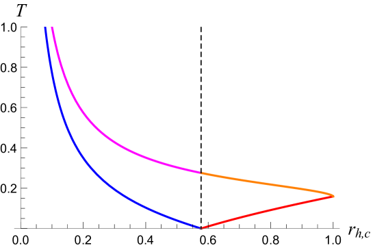
Figure 13: Temperatures of SdS vs. horizon radii $r_{\text{h,c}}$, where we have set $d=4$ and $L_{4}=1$. The blue and red curves correspond to the temperatures $T_{\text{h}}=\kappa_{\text{h}}/2\pi$ and $T_{\text{c}}=\kappa_{\text{c}}/2\pi$, respectively, where the surface gravities are defined with respect to the timelike Killing vector $\xi=\partial_{t}$. The pink and orange curves show the Bousso-Hawking temperatures $\tilde{T}_{\text{h}}=\tilde{\kappa}_{\text{h}}/2\pi$ and $\tilde{T}_{\text{c}}=\tilde{\kappa}_{\text{c}}/2\pi$, respectively, where $\tilde{\kappa}_{\text{h,c}}=\kappa_{\text{h,c}}/\sqrt{f(r_{0})}$ given in (214). Whereas the former temperatures $T_{\text{h,c}}$ vanish for the Nariai black hole with horizon radius $r_{\text{N}}=L_{4}/\sqrt{3}$ (the dashed line), the latter $\tilde{T}_{\text{h,c}}$ are finite and equal to $T_{\text{N}}=\sqrt{3}/2\pi L_{4}$ in the Nariai limit.

$$T_{\text{N}}=\frac{1}{2\pi\hat{L}_{d}}\;.$$ (210)

This temperature can be derived in two-dimensional de Sitter space, for instance, by removing the conical singularity in the Euclidean static patch geometry. It can also be obtained from the higher-dimensional perspective by taking the Nariai limit of the temperatures of the black hole and cosmological horizons. Interestingly, if we normalize the timelike Killing vector of SdS as $\xi=\partial_{t}$, then the temperature of the Nariai black hole vanishes. Namely, for this normalization the (positive) surface gravities of the black hole and cosmological horizon can be found to be

$$\kappa_{\text{h}} =\frac{(d-3)-(d-1)r_{\text{h}}^{2}/L^{2}_{d}}{2r_{\text{h}}}=\frac{r_{\text{N}}^{2}-r_{\text{h}}^{2}}{2r_{\text{h}}\hat{L}_{d}^{2}}\,,$$ (211)

$$\kappa_{\text{c}} =\frac{-(d-3)+(d-1)r_{\text{c}}^{2}/L^{2}_{d}}{2r_{\text{c}}}=\frac{r_{\text{c}}^{2}-r_{\text{N}}^{2}}{2r_{\text{c}}\hat{L}_{d}^{2}}\,.$$

We indeed observe that $\kappa_{\text{h,c}}$ vanishes if $r_{\text{h}}=r_{\text{c}}=r_{\text{N}}.$ However, Bousso and Hawking Bousso:1996au argued that $\xi=\partial_{t}$ is not the correct normalization of the timelike Killing vector of SdS. This is only true for pure de Sitter space, where this choice corresponds to setting $\xi^{2}=-1$ at the origin $r=0$, and for the asymptotically flat Schwarzschild geometry where this normalization yields $\xi^{2}=-1$ at spatial infinity $r=\infty$. These locations in pure de Sitter and Schwarzschild have in common that an observer can stay in place without accelerating. In other words, these radii are maxima of the blackening factor $f(r)$ in the respective spacetimes. Alternatively, for Schwarzschild-de Sitter space the function $f(r)$ attains its maximum when

$$f^{\prime}(r_{0})=0\quad\rightarrow\quad r_{0}^{d-1}=\frac{d-3}{d-2}\frac{8\pi G_{d}ML_{d}^{2}}{\Omega_{d-2}}=\frac{d-3}{2}r_{\text{h,c}}^{d-3}(L^{2}_{d}-r_{\text{h,c}}^{2})\,.$$ (212)

The sphere of radius $r_{0}$ is the place where the cosmological expansion and the black hole attraction cancel each other exactly. The function $f(r)$ at this radius is given by

$$f(r_{0})=1-\frac{d-1}{d-3}\frac{r_{0}^{2}}{L_{d}^{2}}=1-\frac{r_{0}^{2}}{r_{\text{N}}^{2}}\,.$$ (213)

The idea by Bousso and Hawking is now to normalize the Killing vector on the geodesic at fixed radius $r_{0}$, such that $\xi=\frac{1}{\sqrt{f(r_{0})}}\partial_{t}$. This has a similar effect on the surface gravities of the cosmological and black hole horizon

$$\tilde{\kappa}_{\text{h,c}}=\frac{\kappa_{\text{h,c}}}{\sqrt{f(r_{0})}}=\frac{\frac{r_{\text{N}}}{2r_{\text{h,c}}\hat{L}_{d}^{2}}\big{|}r_{\text{N}}^{2}-r_{\text{h,c}}^{2}\big{|}}{\sqrt{r_{\text{N}}^{2}-\left[\frac{d-3}{2}r_{\text{h,c}}^{d-3}(\frac{d-1}{d-3}r_{\text{N}}^{2}-r_{\text{h,c}}^{2})\right]^{2/(d-1)}}}~{}.$$ (214)

Expanding the denominator on the right near $r_{\text{h,c}}=r_{\text{N}}$ gives $\sqrt{r_{\text{N}}^{2}-r_{0}^{2}}\approx\sqrt{d-3}|r_{\text{N}}-r_{\text{h}}|$. Thus, in the Nariai limit we find

$$\tilde{\kappa}_{\text{N}}=\lim_{r_{\text{h,c}}\to r_{\text{N}}}\tilde{\kappa}_{\text{h,c}}=\frac{1}{\hat{L}_{d}}=\frac{\sqrt{d-1}}{L_{d}}\qquad\rightarrow\qquad T_{\text{N}}=\frac{\sqrt{d-1}}{2\pi L_{d}}\,.$$ (215)

This agrees with the expected temperature (210) in two-dimensional de Sitter space.

Appendix C Noether charge formalism for 2D dilaton gravity

To keep this article self contained, here we summarize elements of the Noether charge formalism Wald:1993nt ; Iyer:1994ys in the context of a wide class of two-dimensional dilaton theories of gravity. For a more thorough analysis, see Appendix C of Pedraza:2021cvx .

Lagrangian formalism

Let $\psi=(g_{\mu\nu},\Phi)$ denote a collection of dynamical fields, where $g_{\mu\nu}$ is an arbitrary background metric of a $(1+1)$-dimensional Lorenztian spacetime $M$ and $\Phi$ represents any scalar field on $M$. Consider the following covariant Lagrangian 2-form $L$

$$L=L_{0}\epsilon\left[RZ(\Phi)+U(\Phi)(\nabla\Phi)^{2}-V(\Phi)\right]\;,$$ (216)

where $\epsilon$ is the spacetime volume form, $L_{0}$ is some coupling constant, and $R$ is the Ricci scalar. This is the most general Lagrangian for two-dimensional Einstein gravity coupled non-minimally to a dynamical scalar field, and includes JT gravity and the localized form of the 1-loop Polyakov action. For spacetimes $M$ with boundary $\partial M$, one should also add a boundary Gibbons–Hawking–York 1-form $b$

$$b=-2L_{0}\epsilon_{\partial M}Z(\Phi)K\;.$$ (217)

Here $\epsilon_{\partial M}$ is the volume form on $\partial M$, $K$ is the trace of the extrinsic curvature $K_{\mu\nu}=\frac{1}{2}\mathcal{L}_{n}\gamma_{\mu\nu}$ of the timelike boundary, and $\gamma_{\mu\nu}=-n_{\mu}n_{\nu}+g_{\mu\nu}$ is the induced metric on $\partial M$, with $n_{\mu}$ the (outward pointing) unit normal to $\partial M$.

The symplectic potential 1-form $\theta(\psi,\delta\psi)$ and symplectic current 1-form $\omega(\psi,\delta_{1}\psi,\delta_{2}\psi)\equiv\delta_{1}\theta(\psi,\delta_{2}\psi)-\delta_{2}\theta(\psi,\delta_{1}\psi)$ are, respectively,

$$\theta =L_{0}\epsilon_{\mu}\Big{[}Z(\Phi)(g^{\mu\beta}g^{\alpha\nu}-g^{\mu\nu}g^{\alpha\beta})\nabla_{\nu}\delta g_{\alpha\beta}+(g^{\alpha\beta}\nabla^{\mu}Z(\Phi)$$ (218)

$$-g^{\beta\mu}\nabla^{\alpha}Z(\Phi))\delta g_{\alpha\beta}+2U(\Phi)\nabla^{\mu}\Phi\delta\Phi\Big{]}\;,$$

and

$$\omega =L_{0}\epsilon_{\mu}\Big{[}Z(\Phi)S^{\mu\alpha\beta\nu\rho\sigma}\delta_{1}g_{\rho\sigma}\nabla_{\nu}\delta_{2}g_{\alpha\beta}+\frac{1}{2}g^{\mu\beta}g^{\alpha\nu}g^{\rho\sigma}\delta_{1}g_{\rho\sigma}\delta_{2}g_{\alpha\beta}\nabla_{\nu}Z(\Phi)$$ (219)

$$+(g^{\mu\beta}g^{\alpha\nu}-g^{\mu\nu}g^{\alpha\beta})(\delta_{1}(Z(\Phi))\nabla_{\nu}\delta_{2}g_{\alpha\beta}-\delta_{1}(\nabla_{\nu}Z(\Phi))\delta_{2}g_{\alpha\beta})$$

$$+U(\Phi)\nabla^{\mu}\Phi g^{\alpha\beta}\delta_{1}g_{\alpha\beta}\delta_{2}\Phi+2\delta_{1}(U(\Phi)\nabla^{\mu}\Phi)\delta_{2}\Phi-[1\leftrightarrow 2]\Big{]}\;.$$

Here $Z^{\prime}(\Phi)=\frac{dZ}{d\Phi}$ and $S^{\mu\alpha\beta\nu\rho\sigma}$ is given by

$$S^{\mu\alpha\beta\nu\rho\sigma}=g^{\mu\rho}g^{\alpha\sigma}g^{\beta\nu}-\frac{1}{2}g^{\mu\nu}g^{\alpha\rho}g^{\beta\sigma}-\frac{1}{2}g^{\mu\alpha}g^{\beta\nu}g^{\rho\sigma}-\frac{1}{2}g^{\alpha\beta}g^{\mu\rho}g^{\sigma\nu}+\frac{1}{2}g^{\alpha\beta}g^{\mu\nu}g^{\rho\sigma}\;.$$ (220)

Let $\zeta$ be an arbitrary smooth vector field on $M$ representing an infinitesimal generator of a diffeomorphism. The Noether current 1-form $j_{\zeta}$ associated with $\zeta$ and arbitrary field configuration $\psi$ is defined as $j_{\zeta}\equiv\theta(\psi,\mathcal{L}_{\zeta}\psi)-\zeta\cdot L$, with $\mathcal{L}_{\zeta}$ being the Lie derivative along $\zeta$. The associated Noether charge $0$-form $Q_{\zeta}$ is defined on-shell via $j_{\zeta}=dQ_{\zeta}$. Explicitly, with respect to the theory (216)

$$j_{\zeta}=\epsilon_{\mu}\left[2L_{0}\nabla_{\nu}(Z(\Phi)\nabla^{[\nu}\zeta^{\mu]}+2\zeta^{[\nu}\nabla^{\mu]}Z(\Phi))+2{E^{\mu}}_{\nu}\zeta^{\nu}\right]\;,$$ (221)

$$Q_{\zeta}=-L_{0}\epsilon_{\mu\nu}\left[Z(\Phi)\nabla^{\mu}\zeta^{\nu}+2\zeta^{\mu}\nabla^{\nu}Z(\Phi)\right]\;,$$ (222)

where $\epsilon_{\mu\nu}$ is the volume form for the codimension-0 surface $\partial\Sigma$, which is a cross section of the spatial part of $\partial M$, and $E_{\mu\nu}$ are the metric equations of motion. On-shell, $\omega$, $Q_{\zeta}$ and $\theta$ obey the fundamental variational identity

$$\omega(\psi,\delta\psi,\mathcal{L}_{\zeta}\psi)=d\left[\delta Q_{\zeta}-\zeta\cdot\theta(\psi,\delta\psi)\right]\;.$$ (223)

Hamiltonian formalism

The Hamiltonian $H_{\zeta}$ generating time evolution along the flow of $\zeta$ follows from the variational identity (223). Specifically, let $\Sigma$ be any Cauchy slice of $M$. Denote the induced metric on $\Sigma$ by $h_{\mu\nu}=u_{\mu}u_{\nu}+g_{\mu\nu}$, with $u_{\mu}$ the (future-pointing) unit normal to $\Sigma$. Then, the variation $\delta H_{\zeta}$ and the Hamiltonian itself are given by Harlow:2019yfa ; Pedraza:2021cvx

$$\delta H_{\zeta}=\oint_{\partial\Sigma}[\delta Q_{\zeta}-\zeta\cdot\delta b-\delta C(\psi,\mathcal{L}_{\zeta}\psi)]\;,$$ (224)

$$H_{\zeta}=\int_{\partial\Sigma}[Q_{\zeta}-\zeta\cdot b-C(\psi,\mathcal{L}_{\zeta}\psi)]+\text{cst}\;.$$ (225)

The constant represents a standard ambiguity to the energy of any Hamiltonian system, which we will set to zero. Moreover, $C$ is a local 0-form defined over the boundary $\partial M$ and is covariant under diffeomorphisms preserving the location of the (spatial) boundary $B$ in $\partial M$, and obeys $\theta\big{|}_{B}=\delta b+dC$ if Dirichlet boundary conditions are imposed Harlow:2019yfa . Explicitly,

$$C=c\cdot\epsilon_{\partial M}\;,\quad c^{\mu}=-L_{0}Z(\Phi)\gamma^{\mu\lambda}n^{\nu}\delta g_{\lambda\nu}\;.$$ (226)

For the 2D dilaton-gravity model (216), the terms on the right-hand side of $H_{\zeta}$ pulled back to $\partial\Sigma$ are Pedraza:2021cvx

$$Q_{\zeta}\big{|}_{\partial\Sigma}=+L_{0}\epsilon_{\partial\Sigma}(u_{\mu}n_{\nu}-u_{\nu}n_{\mu})\left[Z(\Phi)\nabla^{\mu}\zeta^{\nu}+2\zeta^{\mu}\nabla^{\nu}Z(\Phi)\right]\;,$$ (227)

$$\zeta\cdot b|_{\partial\Sigma}=-2L_{0}\epsilon_{\partial\Sigma}\zeta^{\mu}u_{\mu}Z(\Phi)K\;,$$ (228)

$$C(\psi,\mathcal{L}_{\zeta}\psi)|_{\partial\Sigma}=-L_{0}\epsilon_{\partial\Sigma}(u^{\mu}n^{\nu}+u^{\nu}n^{\mu})Z(\Phi)\nabla_{\mu}\zeta_{\nu}\;,$$ (229)

where we used $\epsilon_{\mu\nu}|_{\partial\Sigma}=n_{\mu}u_{\nu}-n_{\nu}u_{\mu}$ and $(\epsilon_{\partial M})_{\mu}=+u_{\mu}\epsilon_{\partial\Sigma}$. It follows that the Hamiltonian for $2D$ dilaton gravity is

$$H_{\zeta}=\oint_{\partial\Sigma}\epsilon_{\partial\Sigma}N\varepsilon\;,$$ (230)

with $N=-\zeta^{\mu}u_{\mu}$ being the lapse function and $\varepsilon$ being the quasi-local energy density,

$$\varepsilon\equiv u_{\mu}u_{\nu}\tau^{\mu\nu}=-2L_{0}n^{\alpha}\nabla_{\alpha}Z(\Phi)\;.$$ (231)

Here $\tau_{\mu\nu}\equiv 2L_{0}\gamma_{\mu\nu}n^{\alpha}\nabla_{\alpha}Z(\Phi)$ is the Brown-York stress-energy tensor Brown:1992br .

Appendix D Conformal isometry and diamond universe coordinates

Here we detail the geometry of rectangular causal diamonds in two-dimensional de Sitter space. To accomplish this it is necessary to compute the conformal Killing vectors of $\text{dS}_{2}$, and for completeness we start by deriving the true Killing vectors of $\text{dS}_{2}$. Our approach largely follows Appendices A and B of Pedraza:2021ssc (see also Jacobson:2018ahi ; Visser:2019muv ).

Killing vectors of $\text{dS}_{2}$

A systematic way of deriving the Killing vectors of $\text{dS}_{2}$ is to use the embedding formalism. Two-dimensional de Sitter space can be embedded into three-dimensional Minkowski space $\mathbb{R}^{1,2}$ with line element

$$d\ell^{2}=-(dX^{0})^{2}+(dX^{1})^{2}+(dX^{2})^{2}\,.$$ (232)

dS₂ is a hyperboloid in this embedding space, described by the equation

$$-(X^{0})^{2}+(X^{1})^{2}+(X^{2})^{2}=+L^{2}\;.$$ (233)

The embedding space induces a metric on the hyperboloid, recognized as the metric on $\text{dS}_{2}$. For example, $\text{dS}_{2}$ in static patch coordinates follows from the embedding coordinates

$$X^{0}=\sqrt{L^{2}-r^{2}}\sinh(t/L)\;,\quad X^{1}=r\;,\quad X^{2}=\sqrt{L^{2}-r^{2}}\cosh(t/L)\;,$$ (234)

when $r<L$, while for $r>L$ we have

$$X^{0}=\sqrt{L^{2}-r^{2}}\sinh(t/L)\;,\quad X^{1}=r\;,\quad X^{2}=-\sqrt{L^{2}-r^{2}}\cosh(t/L)\;.$$ (235)

We will be primarily interested in the former case $r<L$, for which (234) in terms of advanced/retarded coordinates $(v,u)$ is

$$X^{0}=L\frac{\sinh\left(\frac{v+u}{2L}\right)}{\cosh\left(\frac{v-u}{2L}\right)}\;,\quad X^{1}=L\frac{\sinh\left(\frac{v-u}{2L}\right)}{\cosh\left(\frac{v-u}{2L}\right)}\;,\quad X^{2}=L\frac{\cosh\left(\frac{v+u}{2L}\right)}{\cosh\left(\frac{v-u}{2L}\right)}\;.$$ (236)

The isometry group of Lorentzian $\text{dS}_{2}$ is $O(1,2)$ with $\frac{1}{2}(2)(2+1)=3$ Killing vectors. With respect to the embedding coordinates the single rotation generator $J$ and the two boost generators $B_{1,2}$ of the isometry group are

$$J=X^{1}\partial_{X^{2}}-X^{2}\partial_{X^{1}}\;,\quad B_{1}=X^{1}\partial_{X^{0}}+X^{0}\partial_{X^{1}}\;,\quad B_{2}=X^{2}\partial_{X^{0}}+X^{0}\partial_{X^{2}}\;,$$ (237)

obeying the algebra

$$[J,B_{1}]=-B_{2}\;,\quad[J,B_{2}]=B_{1}\;,\quad[B_{1},B_{2}]=J\;.$$ (238)

Substituting the embedding coordinates (234) into the generators (237) yields the true Killing vectors of $\text{dS}_{2}$ in static patch coordinates:

$$\begin{split}&J=-\frac{rL}{\sqrt{L^{2}-r^{2}}}\sinh(t/L)\partial_{t}-\sqrt{L^{2}-r^{2}}\cosh(t/L)\partial_{r}\;,\\ &B_{1}=\frac{rL}{\sqrt{L^{2}-r^{2}}}\cosh(t/L)\partial_{t}+\sqrt{L^{2}-r^{2}}\sinh(t/L)\partial_{r}\;,\quad B_{2}=L\partial_{t}\;.\end{split}$$ (239)

We see the boost $B_{2}$ generates time translations in the static patch. Alternatively, the generators in null coordinates $(v,u)$ are

$$\begin{split}&J=L[\cosh(u/L)\partial_{u}-\cosh(v/L)\partial_{v}]\;,\\ &B_{1}=L[\sinh(v/L)\partial_{v}-\sinh(u/L)\partial_{u}]\;,\quad B_{2}=L(\partial_{v}+\partial_{u})\;.\end{split}$$ (240)

Conformal Killing vectors of causal diamonds in $\text{dS}_{2}$

Consider a rectangular causal diamond in a generic two-dimensional spacetime in conformal gauge $d\ell^{2}=-e^{2\rho}dudv$, as described in Section 4. The conformal isometry of such a diamond is generated by Pedraza:2021ssc

$$\zeta=A_{a}(u-u_{0})\partial_{u}+A_{b}(v-v_{0})\partial_{v}\,,\quad A_{j}(y)=g_{j}(y)[h(j)-h(y)]\;,$$ (241)

where $g$ and $h$ are even functions, and $j$ is a length scale taking the values $a$ or $b$. The conformal Killing vector field $\zeta$ is constructed by demanding it respects the reflection symmetries across the maximal slice $\Sigma$ and the line intersecting past and future vertices when $a$ and $b$ are interchanged. Furthermore, we require that $\zeta$ maps the diamond onto itself, i.e., $\zeta$ must be tangent to the null generators of the null boundaries, imposing $A_{j}(\pm j)=0$. This implies that the past and future null boundaries are conformal Killing horizons.

Generally, the length scales $a$ and $b$ are different, leading to two positive surface gravities,

$$\kappa_{a}=g_{a}(a)h^{\prime}(a)\,,\quad\quad\kappa_{b}=g_{b}(b)h^{\prime}(b)\,,$$ (242)

defined via $\nabla_{\mu}\zeta^{2}=-2\kappa\zeta_{\mu}$, evaluated on the future null boundaries $u-u_{0}=a$ and $v-v_{0}=b$, respectively. The prime denotes the derivative with respect to $y$ (denoting $u$ and $v$ respectively). The surface gravities are constant and hence they satisfy the zeroth law for bifurcate conformal Killing horizons proven in Appendix C of Jacobson:2018ahi .

Furthermore, for square causal diamonds (when $a=b$) there is only a single surface gravity $\kappa$, and the conformal Killing vector becomes approximately a boost Killing vector near the bifurcation surface of the horizon

$$\zeta\approx g(a)h^{\prime}(a)\left[\tilde{v}\partial_{\tilde{v}}-\tilde{u}\partial_{\tilde{u}}\right]\qquad\text{at}\qquad\tilde{u}=\tilde{v}=0\,,$$ (243)

with $\tilde{u}\equiv u-u_{0}-a$ and $\tilde{v}\equiv v-v_{0}+a$. The vector field between brackets is the boost Killing vector in null coordinates in flat space, and we regonize the normalization as being the surface gravity in (242).

We can restrict the form of $\zeta$ in (241) further by placing the diamond in two-dimensional de Sitter space and requiring that $\zeta$ become the generator of time translations when the causal diamond coincides with the static patch (the maximal diamond). First, we express the conformal Killing vector in terms of Kruskal coordinates $(U,V)=(-Le^{-u/L},Le^{v/L})$, and set $u_{0}=v_{0}=0$ and $a=b=-L\log(B/L)$ for simplicity,

$$\zeta=\frac{1}{L}\left[A(V)V\partial_{V}-A(U)U\partial_{U}\right]\,,\qquad A(Y)=\frac{\kappa L}{B^{-1}h^{\prime}(B^{-1})}\frac{g(Y)}{g(B)}\big{[}h(B)-h(Y)\big{]}\,,$$ (244)

where now the prime denotes the derivative with respect to $Y$, denoting $U$ and $V$ respectively. Further, the functions $g$ and $h$ satisfy $g(Y)=g(Y^{-1})$ and $h(Y)=h(Y^{-1})$. Next, we require that in the maximal diamond limit ($a,b\to\infty$ or $B\to 0$) we have

$$\lim_{B\to 0}\zeta=\kappa(V\partial_{V}-U\partial_{U})=\kappa B_{2}\,,$$ (245)

where $B_{2}$ is the time translation generator in (240). This implies

$$g(Y)=1,\qquad\lim_{B\to 0}\frac{Bh(B)}{h^{\prime}(B^{-1})}=1,\qquad\lim_{B\to 0}\frac{C}{h^{\prime}(B^{-1})}=0\,.$$ (246)

Assuming the function $h(B)$ can be expanded as

$$h(B)=\sum_{n=-\infty}^{n=\infty}a_{n}B^{n}\,$$ (247)

with $a_{n}=a_{-n}$, since $h(B)=h(B^{-1})$. The second condition in (246) implies $a_{n}=0$ for $n>1$, hence only $a_{0}$ and $a_{1}$ are nonvanishing. Therefore, we arrive at the unique form for the conformal Killing vector by inserting $g(Y)=1$ and $h(Y)=a_{1}Y^{-1}+a_{0}+a_{1}Y$ into (244)

$$\zeta=\frac{1}{L}\left[A(V)V\partial_{V}-A(U)U\partial_{U}\right]\,,\qquad A(Y)=\kappa L\frac{1+B^{2}}{1-B^{2}}\left[1-\frac{Y+Y^{-1}}{B+B^{-1}}\right]\,.$$ (248)

Transforming back to static null coordinates using (34) yields

$$\zeta=A(u)\partial_{u}+A(v)\partial_{v}\,,\qquad A(y)=\frac{\kappa L}{\sinh(a/L)}\left[\cosh(a/L)-\cosh(y/L)\right]\,.$$ (249)

This is the expected result since it is identical to the conformal Killing vector of a spherically symmetric causal diamond in $d$-dimensional de Sitter space Jacobson:2018ahi . In higher dimensions, however, the spherical symmetry of a diamond restricts the form of the conformal Killing vector uniquely, whereas in $d=2$ we need the additional requirement (245) to arrive at the same unique form. For a rectangular diamond in $\text{dS}_{2}$ centered at $(u_{0},v_{0})$ this generalizes to

$$\zeta=A_{a}(u-u_{0})\partial_{u}+A_{b}(v-v_{0})\partial_{v}\;,\quad A_{a}(y)=\frac{\kappa_{a}L}{\sinh(a/L)}\left[\cosh(a/L)-\cosh(y/L)\right]\;,$$ (250)

and similarly for $A_{b}(y)$. It is straightforward to verify $\zeta$ is a conformal Killing vector, obeying the conformal Killing equation, $2\nabla_{(\mu}\zeta_{\nu)}=(\nabla\cdot\zeta)g_{\mu\nu}$. Incidentally, the expression (250) is equivalent to the form of the conformal Killing vector preserving a causal diamond in $\text{AdS}_{2}$ when we set $\mu=-1$ and $L\to iL$ in equation (A7) of Pedraza:2021ssc . To summarize, the maximal diamond in the de Sitter static patch (which is the static patch itself) admits a true isometry, whereas finite causal diamonds only admit a conformal isometry generated by (250).

Diamond universe coordinates

We now introduce inextendible coordinates $(s,x)$ adapted to the flow of $\zeta$ that cover the causal diamond Jacobson:2018ahi . The coordinate $s$ is the conformal Killing time defined such that $\zeta\cdot ds=1$ and, for $a=b$, $s=0$ on the maximal slice $\Sigma$ and has the range $s\in[-\infty,\infty]$. Similarly, the spatial coordinate $x\in[-\infty,\infty]$ obeys $\zeta\cdot dx=0$ and $|dx|=|ds|$ and, for $a=b$, the origin $x=0$ is at $r_{*}=r_{*,0}\equiv\frac{1}{2}(v_{0}-u_{0})$. From these conditions, the two-dimensional line element in so-called “diamond universe” coordinates is

$$d\ell^{2}=C^{2}(s,x)(-ds^{2}+dx^{2})=-C^{2}(\bar{u},\bar{v})d\bar{u}d\bar{v}\,,$$ (251)

with null coordinates, $\bar{u}=s-x$ and $\bar{v}=s+x$, and $C^{2}$ is a conformal factor determined below. In these coordinates, the null boundaries of the diamond are located at $\bar{u}=\pm\infty$ ($u-u_{0}=\pm a$) and $\bar{v}=\pm\infty$ ($v-v_{0}=\pm b$).

From the line element (251), it is clear $\zeta=\partial_{s}=\partial_{\bar{u}}+\partial_{\bar{v}}$ is a conformal Killing vector, which should be equivalent to the vector field (250) preserving the diamond in $\text{dS}_{2}$. Setting the expression (250) for $\zeta$ equal to $\partial_{\bar{u}}+\partial_{\bar{v}}$ yields the following transformation between null coordinates $(\bar{u},\bar{v})$ and $(u,v)$ Pedraza:2021ssc

$$\begin{split}e^{(u-u_{0})/L}=\frac{\cosh\left[(a/L+\kappa_{a}\bar{u})/2\right]}{\cosh\left[(a/L-\kappa_{a}\bar{u})/2\right]}\,,\quad e^{(v-v_{0})/L}=\frac{\cosh\left[(b/L+\kappa_{b}\bar{v})/2\right]}{\cosh\left[(b/L-\kappa_{b}\bar{v})/2\right]}\,.\end{split}$$ (252)

With this coordinate transformation, we uncover the conformal factor $C^{2}(\bar{u},\bar{v})$ by comparing line elements (33) and (251),

$$C^{2}(\bar{u},\bar{v})=\frac{4\kappa_{a}\kappa_{b}L^{2}e^{\kappa_{a}\bar{u}+\kappa_{b}\bar{v}+2r_{\ast,0}/L}\left(e^{2b/L}-1\right)\left(e^{2a/L}-1\right)}{\left[\left(e^{b/L}+e^{\kappa_{b}\bar{v}}\right)\left(e^{a/L+\kappa_{a}\bar{u}}+1\right)+e^{2r_{\ast,0}/L}\left(e^{a/L}+e^{\kappa_{a}\bar{u}}\right)\left(e^{b/L+\kappa_{b}\bar{v}}+1\right)\right]^{2}}\;.$$ (253)

For the special case $v_{0}=u_{0}$ and $a=b$, the (square root of the) conformal factor reduces to

$$C(s,x)=\frac{\kappa L\sinh(a/L)}{\cosh(a/L)\cosh(\kappa x)+\cosh(\kappa s)}\,.$$ (254)

This is the conformal factor for a spherically symmetric causal diamond in higher-dimensional de Sitter space centered at $r_{0}=0$, see equation (B5) in Jacobson:2018ahi (where we have set $\kappa=1$). Furthermore, for a maximal diamond we see that the conformal factor (254) becomes identical to the conformal factor of the static patch itself given in (33), i.e., in the limit $a,b\to\infty$ and $v_{0}\to u_{0}$ we have $C\to\kappa L\text{sech}(\kappa x)$.

Euclidean continuation of causal diamonds

Ultimately we are interested in the Euclideanized diamond, where we Wick rotate the diamond time $s\to-is_{\text{E}}$. In diamond universe coordinates, the line element (251) becomes

$$d\ell^{2}=C^{2}(s_{\text{E}},x)(ds_{\text{E}}^{2}+dx^{2})\;,$$ (255)

where $s_{\text{E}}$ is periodic in $2\pi/\kappa$, so as to remove the conical singularity in the Euclidean spacetime due to the horizon. To visualize the Euclidean diamond, it is convenient to introduce a set of Kruskal coordinates

$$T_{\text{K}}=\frac{1}{2}(V+U)\;,\quad X_{\text{K}}=\frac{1}{2}(V-U)\;,$$ (256)

with $U=-Le^{-u/L}$ and $V=Le^{v/L}$. For convenience, consider the case when $u_{0}=v_{0}=0$ and $a=b$, where the conformal factor $C(s,x)$ is given by (254). From the coordinate transformation (252), we have

$$T_{\text{K}}=\frac{L\sinh(a/L)\sinh(\kappa s)}{\cosh(\kappa s)+\cosh(a/L-\kappa x)}\;,\quad X_{\text{K}}=\frac{L\left(\cosh(a/L)\cosh(\kappa s)+\cosh(\kappa x)\right)}{\cosh(\kappa s)+\cosh(a/L-\kappa x)}\;.$$ (257)

Upon Wick rotating the conformal Killing time $s$, we have

$$T_{\text{K}}\to-i\frac{L\sinh(a/L)\sin(\kappa s_{\text{E}})}{\cos(\kappa s_{\text{E}})+\cosh(a/L-\kappa x)}\equiv-iT_{\text{K}}^{\text{E}}\;,$$ (258)

$$X_{\text{K}}\to\frac{L\left(\cosh(a/L)\cos(\kappa s_{\text{E}})+\cosh(\kappa x)\right)}{\cos(\kappa s_{\text{E}})+\cosh(a/L-\kappa x)}\;.$$

Remarkably, as realized in higher-dimensional black hole geometries Banks:2005bm and in $\text{AdS}_{2}$ Pedraza:2021ssc , the Euclidean continuation of the finite causal diamond covers nearly all of Euclidean $\text{dS}_{2}$. The only difference is that the Euclidean diamond spacetime has two punctures corresponding to the horizons at $x\to\pm\infty$, as visualized in Figure 9. For the square diamond, the punctures at $x\to\pm\infty$ are mapped to the points $(T_{\text{K}}^{\text{E}},X_{\text{K}})=(0,Le^{\pm a/L})$.

References

- (1) G. W. Gibbons and S. W. Hawking, Cosmological Event Horizons, Thermodynamics, and Particle Creation, Phys. Rev. D 15 (1977) 2738–2751.
- (2) T. Banks, Cosmological breaking of supersymmetry?, Int. J. Mod. Phys. A 16 (2001) 910–921, [hep-th/0007146].
- (3) E. Witten, Quantum gravity in de Sitter space, in Strings 2001: International Conference, 6, 2001. hep-th/0106109.
- (4) M. Spradlin, A. Strominger and A. Volovich, Les Houches lectures on de Sitter space, in Les Houches Summer School: Session 76: Euro Summer School on Unity of Fundamental Physics: Gravity, Gauge Theory and Strings, pp. 423–453, 10, 2001. hep-th/0110007.
- (5) N. Goheer, M. Kleban and L. Susskind, The Trouble with de Sitter space, JHEP 07 (2003) 056, [hep-th/0212209].
- (6) D. Anninos, De Sitter Musings, Int. J. Mod. Phys. A 27 (2012) 1230013, [1205.3855].
- (7) A. Strominger, The dS / CFT correspondence, JHEP 10 (2001) 034, [hep-th/0106113].
- (8) J. M. Maldacena, Non-Gaussian features of primordial fluctuations in single field inflationary models, JHEP 05 (2003) 013, [astro-ph/0210603].
- (9) D. Anninos, T. Hartman and A. Strominger, Higher Spin Realization of the dS/CFT Correspondence, Class. Quant. Grav. 34 (2017) 015009, [1108.5735].
- (10) D. Anninos, F. Denef, R. Monten and Z. Sun, Higher Spin de Sitter Hilbert Space, JHEP 10 (2019) 071, [1711.10037].
- (11) T. Banks, Some thoughts on the quantum theory of stable de Sitter space, hep-th/0503066.
- (12) M. K. Parikh and E. P. Verlinde, De Sitter holography with a finite number of states, JHEP 01 (2005) 054, [hep-th/0410227].
- (13) D. Anninos, S. A. Hartnoll and D. M. Hofman, Static Patch Solipsism: Conformal Symmetry of the de Sitter Worldline, Class. Quant. Grav. 29 (2012) 075002, [1109.4942].
- (14) D. Anninos and D. M. Hofman, Infrared Realization of dS2 in AdS2, Class. Quant. Grav. 35 (2018) 085003, [1703.04622].
- (15) S. Leuven, E. Verlinde and M. Visser, Towards non-AdS Holography via the Long String Phenomenon, JHEP 06 (2018) 097, [1801.02589].
- (16) L. Susskind, De Sitter Holography: Fluctuations, Anomalous Symmetry, and Wormholes, Universe 7 (2021) 464, [2106.03964].
- (17) L. Susskind, Black Holes Hint Towards De Sitter-Matrix Theory, 2109.01322.
- (18) L. Susskind, Entanglement and Chaos in De Sitter Holography: An SYK Example, 2109.14104.
- (19) E. Shaghoulian, The central dogma and cosmological horizons, 2110.13210.
- (20) E. Shaghoulian and L. Susskind, Entanglement in De Sitter Space, 2201.03603.
- (21) R. Jackiw, Lower Dimensional Gravity, Nucl. Phys. B 252 (1985) 343–356.
- (22) C. Teitelboim, Gravitation and Hamiltonian Structure in Two Space-Time Dimensions, Phys. Lett. B 126 (1983) 41–45.
- (23) W. Sybesma, Pure de Sitter space and the island moving back in time, 2008.07994.
- (24) L. Aalsma and W. Sybesma, The Price of Curiosity: Information Recovery in de Sitter Space, JHEP 05 (2021) 291, [2104.00006].
- (25) J. W. York, Jr., Black hole thermodynamics and the Euclidean Einstein action, Phys. Rev. D 33 (1986) 2092–2099.
- (26) B. F. Whiting and J. W. York, Action principle and partition function for the gravitational field in black-hole topologies, Phys. Rev. Lett. 61 (Sep, 1988) 1336–1339.
- (27) J. D. Brown, G. L. Comer, E. A. Martinez, J. Melmed, B. F. Whiting and J. W. York, Jr., Thermodynamic Ensembles and Gravitation, Class. Quant. Grav. 7 (1990) 1433–1444.
- (28) J. D. Brown and J. W. York, Jr., Quasilocal energy and conserved charges derived from the gravitational action, Phys. Rev. D 47 (1993) 1407–1419, [gr-qc/9209012].
- (29) A. M. Polyakov, Quantum Geometry of Bosonic Strings, Phys. Lett. B 103 (1981) 207–210.
- (30) J. F. Pedraza, A. Svesko, W. Sybesma and M. R. Visser, Semi-classical thermodynamics of quantum extremal surfaces in Jackiw-Teitelboim gravity, 2107.10358.
- (31) J. D. Bekenstein, Generalized second law of thermodynamics in black hole physics, Phys. Rev. D 9 (1974) 3292–3300.
- (32) N. Engelhardt and A. C. Wall, Quantum Extremal Surfaces: Holographic Entanglement Entropy beyond the Classical Regime, JHEP 01 (2015) 073, [1408.3203].
- (33) T. Faulkner, A. Lewkowycz and J. Maldacena, Quantum corrections to holographic entanglement entropy, JHEP 11 (2013) 074, [1307.2892].
- (34) S. Ryu and T. Takayanagi, Holographic derivation of entanglement entropy from AdS/CFT, Phys. Rev. Lett. 96 (2006) 181602, [hep-th/0603001].
- (35) V. E. Hubeny, M. Rangamani and T. Takayanagi, A Covariant holographic entanglement entropy proposal, JHEP 07 (2007) 062, [0705.0016].
- (36) A. Almheiri, R. Mahajan, J. Maldacena and Y. Zhao, The Page curve of Hawking radiation from semiclassical geometry, JHEP 03 (2020) 149, [1908.10996].
- (37) G. Penington, Entanglement Wedge Reconstruction and the Information Paradox, JHEP 09 (2020) 002, [1905.08255].
- (38) A. Almheiri, N. Engelhardt, D. Marolf and H. Maxfield, The entropy of bulk quantum fields and the entanglement wedge of an evaporating black hole, JHEP 12 (2019) 063, [1905.08762].
- (39) A. Almheiri, R. Mahajan and J. Maldacena, Islands outside the horizon, 1910.11077.
- (40) J. D. Bekenstein, A Universal Upper Bound on the Entropy to Energy Ratio for Bounded Systems, Phys. Rev. D 23 (1981) 287.
- (41) W. Fischler and L. Susskind, Holography and cosmology, hep-th/9806039.
- (42) N. Arkani-Hamed, S. Dubovsky, A. Nicolis, E. Trincherini and G. Villadoro, A Measure of de Sitter entropy and eternal inflation, JHEP 05 (2007) 055, [0704.1814].
- (43) T. Hartman, Y. Jiang and E. Shaghoulian, Islands in cosmology, 2008.01022.
- (44) V. Balasubramanian, A. Kar and T. Ugajin, Entanglement between two disjoint universes, JHEP 02 (2021) 136, [2008.05274].
- (45) V. Balasubramanian, A. Kar and T. Ugajin, Islands in de Sitter space, JHEP 02 (2021) 072, [2008.05275].
- (46) J. Kames-King, E. Verheijden and E. Verlinde, No Page Curves for the de Sitter Horizon, 2108.09318.
- (47) D. Teresi, Islands and the de Sitter entropy bound, 2112.03922.
- (48) A. Lewkowycz and J. Maldacena, Generalized gravitational entropy, JHEP 08 (2013) 090, [1304.4926].
- (49) X. Dong and A. Lewkowycz, Entropy, Extremality, Euclidean Variations, and the Equations of Motion, JHEP 01 (2018) 081, [1705.08453].
- (50) A. Almheiri, T. Hartman, J. Maldacena, E. Shaghoulian and A. Tajdini, Replica Wormholes and the Entropy of Hawking Radiation, JHEP 05 (2020) 013, [1911.12333].
- (51) G. Penington, S. H. Shenker, D. Stanford and Z. Yang, Replica wormholes and the black hole interior, 1911.11977.
- (52) J. D. Brown and J. W. York, Jr., The Microcanonical functional integral. 1. The Gravitational field, Phys. Rev. D 47 (1993) 1420–1431, [gr-qc/9209014].
- (53) M. Banados, C. Teitelboim and J. Zanelli, Black hole entropy and the dimensional continuation of the Gauss-Bonnet theorem, Phys. Rev. Lett. 72 (1994) 957–960, [gr-qc/9309026].
- (54) J. F. Pedraza, A. Svesko, W. Sybesma and M. R. Visser, Microcanonical Action and the Entropy of Hawking Radiation, 2111.06912.
- (55) A. Achucarro and M. E. Ortiz, Relating black holes in two-dimensions and three-dimensions, Phys. Rev. D 48 (1993) 3600–3605, [hep-th/9304068].
- (56) A. Fabbri, D. J. Navarro and J. Navarro-Salas, Quantum evolution of near extremal Reissner-Nordstrom black holes, Nucl. Phys. B 595 (2001) 381–401, [hep-th/0006035].
- (57) P. Nayak, A. Shukla, R. M. Soni, S. P. Trivedi and V. Vishal, On the Dynamics of Near-Extremal Black Holes, JHEP 09 (2018) 048, [1802.09547].
- (58) S. Sachdev, Universal low temperature theory of charged black holes with AdS2 horizons, J. Math. Phys. 60 (2019) 052303, [1902.04078].
- (59) E. Verheijden and E. Verlinde, From the BTZ black hole to JT gravity: geometrizing the island, JHEP 11 (2021) 092, [2102.00922].
- (60) J. Cotler, K. Jensen and A. Maloney, Low-dimensional de Sitter quantum gravity, JHEP 06 (2020) 048, [1905.03780].
- (61) J. Maldacena, G. J. Turiaci and Z. Yang, Two dimensional Nearly de Sitter gravity, JHEP 01 (2021) 139, [1904.01911].
- (62) H. Maxfield and G. J. Turiaci, The path integral of 3D gravity near extremality; or, JT gravity with defects as a matrix integral, JHEP 01 (2021) 118, [2006.11317].
- (63) R. M. Wald, Black hole entropy is the Noether charge, Phys. Rev. D 48 (1993) R3427–R3431, [gr-qc/9307038].
- (64) H. Nariai, On a New Cosmological Solution of Einstein’s Field Equations of Gravitation, General Relativity and Gravitation 31 (June, 1999) 963.
- (65) Y. Sekiwa, Thermodynamics of de Sitter black holes: Thermal cosmological constant, Phys. Rev. D 73 (2006) 084009, [hep-th/0602269].
- (66) B. P. Dolan, D. Kastor, D. Kubiznak, R. B. Mann and J. Traschen, Thermodynamic Volumes and Isoperimetric Inequalities for de Sitter Black Holes, Phys. Rev. D 87 (2013) 104017, [1301.5926].
- (67) D. Kastor, S. Ray and J. Traschen, Enthalpy and the Mechanics of AdS Black Holes, Class. Quant. Grav. 26 (2009) 195011, [0904.2765].
- (68) T. Jacobson and M. Visser, Gravitational Thermodynamics of Causal Diamonds in (A)dS, SciPost Phys. 7 (2019) 079, [1812.01596].
- (69) P. H. Ginsparg and M. J. Perry, Semiclassical Perdurance of de Sitter Space, Nucl. Phys. B 222 (1983) 245–268.
- (70) F. Rosso and A. Svesko, Novel aspects of the extended first law of entanglement, JHEP 08 (2020) 008, [2003.10462].
- (71) V. Balasubramanian, J. de Boer and D. Minic, Mass, entropy and holography in asymptotically de Sitter spaces, Phys. Rev. D 65 (2002) 123508, [hep-th/0110108].
- (72) D. Anninos, G. S. Ng and A. Strominger, Asymptotic Symmetries and Charges in De Sitter Space, Class. Quant. Grav. 28 (2011) 175019, [1009.4730].
- (73) G. W. Gibbons and S. W. Hawking, Action Integrals and Partition Functions in Quantum Gravity, Phys. Rev. D 15 (1977) 2752–2756.
- (74) B. Banihashemi and T. Jacobson, Thermodynamic ensembles with cosmological horizons, 2204.05324.
- (75) J. D. E. Creighton and R. B. Mann, Quasilocal thermodynamics of two-dimensional black holes, Phys. Rev. D 54 (1996) 7476–7482.
- (76) J. P. S. Lemos, Thermodynamics of the two-dimensional black hole in the Teitelboim-Jackiw theory, Phys. Rev. D 54 (1996) 6206–6212, [gr-qc/9608016].
- (77) P. Draper and S. Farkas, Euclidean de Sitter Black Holes and Microcanonical Equilibrium, 2203.01871.
- (78) V. Iyer and R. M. Wald, Some properties of Noether charge and a proposal for dynamical black hole entropy, Phys. Rev. D 50 (1994) 846–864, [gr-qc/9403028].
- (79) S. Liberati and C. Pacilio, Smarr Formula for Lovelock Black Holes: a Lagrangian approach, Phys. Rev. D 93 (2016) 084044, [1511.05446].
- (80) S. M. Christensen and S. A. Fulling, Trace Anomalies and the Hawking Effect, Phys. Rev. D 15 (1977) 2088–2104.
- (81) T. M. Fiola, J. Preskill, A. Strominger and S. P. Trivedi, Black hole thermodynamics and information loss in two-dimensions, Phys. Rev. D 50 (1994) 3987–4014, [hep-th/9403137].
- (82) L. Susskind and J. Uglum, Black hole entropy in canonical quantum gravity and superstring theory, Phys. Rev. D 50 (1994) 2700–2711, [hep-th/9401070].
- (83) T. Jacobson, Black hole entropy and induced gravity, gr-qc/9404039.
- (84) R. C. Myers, Black hole entropy in two-dimensions, Phys. Rev. D 50 (1994) 6412–6421, [hep-th/9405162].
- (85) K. Goto, T. Hartman and A. Tajdini, Replica wormholes for an evaporating 2D black hole, JHEP 04 (2021) 289, [2011.09043].
- (86) V. Iyer and R. M. Wald, A Comparison of Noether charge and Euclidean methods for computing the entropy of stationary black holes, Phys. Rev. D 52 (1995) 4430–4439, [gr-qc/9503052].
- (87) J. D. Brown, Black hole entropy and the Hamiltonian formulation of diffeomorphism invariant theories, Phys. Rev. D 52 (1995) 7011–7026, [gr-qc/9506085].
- (88) T. Jacobson, Entanglement Equilibrium and the Einstein Equation, Phys. Rev. Lett. 116 (2016) 201101, [1505.04753].
- (89) M. R. Visser, Emergent gravity in a holographic universe. PhD thesis, Amsterdam U., 2019. 1908.05469.
- (90) T. Banks, P. Draper and S. Farkas, Path Integrals for Causal Diamonds and the Covariant Entropy Principle, Phys. Rev. D 103 (2021) 106022, [2008.03449].
- (91) T. Anous, J. Kruthoff and R. Mahajan, Density matrices in quantum gravity, SciPost Phys. 9 (2020) 045, [2006.17000].
- (92) Y. Chen, V. Gorbenko and J. Maldacena, Bra-ket wormholes in gravitationally prepared states, JHEP 02 (2021) 009, [2007.16091].
- (93) R. Emparan, J. F. Pedraza, A. Svesko, M. Tomašević and M. R. Visser, Black holes in dS3, 2207.03302.
- (94) D. Anninos and B. Mühlmann, The semiclassical gravitational path integral and random matrices (toward a microscopic picture of a dS2 universe), JHEP 12 (2021) 206, [2111.05344].
- (95) F. Sanches and S. J. Weinberg, Holographic entanglement entropy conjecture for general spacetimes, Phys. Rev. D 94 (2016) 084034, [1603.05250].
- (96) Y. Nomura, P. Rath and N. Salzetta, Spacetime from Unentanglement, Phys. Rev. D 97 (2018) 106010, [1711.05263].
- (97) J. Maldacena, D. Stanford and Z. Yang, Conformal symmetry and its breaking in two dimensional Nearly Anti-de-Sitter space, PTEP 2016 (2016) 12C104, [1606.01857].
- (98) L. V. Iliesiu, J. Kruthoff, G. J. Turiaci and H. Verlinde, JT gravity at finite cutoff, SciPost Phys. 9 (2020) 023, [2004.07242].
- (99) V. Gorbenko, E. Silverstein and G. Torroba, dS/dS and , JHEP 03 (2019) 085, [1811.07965].
- (100) E. Coleman, E. A. Mazenc, V. Shyam, E. Silverstein, R. M. Soni, G. Torroba et al., de Sitter Microstates from and the Hawking-Page Transition, 2110.14670.
- (101) S. E. Aguilar-Gutierrez, A. Chatwin-Davies, T. Hertog, N. Pinzani-Fokeeva and B. Robinson, Islands in multiverse models, JHEP 11 (2021) 212, [2108.01278].
- (102) L. Aalsma, M. Parikh and J. P. Van Der Schaar, Back(reaction) to the Future in the Unruh-de Sitter State, JHEP 11 (2019) 136, [1905.02714].
- (103) D. Grumiller, Quantum dilaton gravity in two-dimensions with matter, other thesis, 5, 2001.
- (104) K. Narayan, Aspects of two-dimensional dilaton gravity, dimensional reduction, and holography, Phys. Rev. D 104 (2021) 026007, [2010.12955].
- (105) U. Moitra, S. K. Sake and S. P. Trivedi, Aspects of Jackiw-Teitelboim Gravity in Anti-de Sitter and de Sitter spacetime, 2202.03130.
- (106) V. Cardoso, O. J. C. Dias and J. P. S. Lemos, Nariai, Bertotti-Robinson and anti-Nariai solutions in higher dimensions, Phys. Rev. D 70 (2004) 024002, [hep-th/0401192].
- (107) R. Bousso and S. W. Hawking, Pair creation of black holes during inflation, Phys. Rev. D 54 (1996) 6312–6322, [gr-qc/9606052].
- (108) D. Harlow and J.-Q. Wu, Covariant phase space with boundaries, JHEP 10 (2020) 146, [1906.08616].