A General Framework for Distributed Partitioned Optimization

Abstract

Distributed optimization is widely used in large scale and privacy preserving machine learning and various distributed control and sensing systems. It is assumed that every agent in the network possesses a local objective function, and the nodes interact via a communication network. In the standard scenario, which is mostly studied in the literature, the local functions are dependent on a common set of variables, and, therefore, have to send the whole variable set at each communication round. In this work, we study a different problem statement, where each of the local functions held by the nodes depends only on some subset of the variables. Given a network, we build a general algorithm-independent framework for distributed partitioned optimization that allows to construct algorithms with reduced communication load using a generalization of Laplacian matrix. Moreover, our framework allows to obtain algorithms with non-asymptotic convergence rates with explicit dependence on the parameters of the network, including accelerated and optimal first-order methods. We illustrate the efficacy of our approach on a synthetic example.

1 Introduction

Distributed algorithms is a classical Borkar and Varaiya (1982); Tsitsiklis and Athans (1984); DeGroot (1974), yet actively developing research area with many applications including robotics, resource allocation, power system control, control of drone or satellite networks, distributed statistical inference and optimal transport, multiagent reinforcement learning Xiao and Boyd (2006); Rabbat and Nowak (2004); Ram et al. (2009); Kraska et al. (2013); Uribe et al. (2018); Kroshnin et al. (2019); Ivanova et al. (2020). Recent surge of interest to such problems in optimization and machine learning is motivated by large-scale learning problems with privacy constraints and other challenges such as data being produced or stored distributedly Bottou (2010); Boyd et al. (2011); Nedić et al. (2017). An important part of this research studies distributed optimization algorithms over arbitrary networks of computing agents, e.g. sensors or computers, which is represented by a connected graph in which two agents can communicate with each other if there is an edge between them. This imposes communication constraints and the goal of the whole system Nedić et al. (2009) is to cooperatively minimize a global objective using only local communications between agents, each of which has access only to a local piece of the global objective.

In this paper, we further exploit additional structure in such problems and consider distributed partitioned optimization problems also known as optimization with overlapping variables and distributed optimization of partially separable objective functions. Such problems arise in many modern big-data applications, e.g., distributed matrix completion, distributed estimation in power networks, network utility maximization, distributed resource allocation, cooperative localization in wireless networks, building maps by robotic networks Erseghe (2012); Kekatos and Giannakis (2012); Carli and Notarstefano (2013); Notarnicola et al. (2017); Cannelli et al. (2020). As in the standard formulations, the goal is to minimize a sum of $m$ functions $\tilde{f}_{i}(x)$, $i=1,...,m$ with each $\tilde{f}_{i}(x)$ stored at a node of the computational network. Yet, unlike standard distributed problems, the space of decision variables is divided into $n$ blocks, and each of $\tilde{f}_{i}(x)$ may depend only on a, possibly small, subset of blocks. Such sparse structure leads to inefficiency of the standard approaches Scaman et al. (2017); Kovalev et al. (2020) since they require each node to store and send the whole vector of variables instead of storing and exchanging with other nodes a small vector of variables which influences its local objective $\tilde{f}_{i}(x)$. This leads to inefficient usage of computational and communication resources.

Theory of algorithms exploiting such additional structure seems to be underdeveloped in the literature. Necoara and Clipici (2016) propose a parallel version of a randomized (block) coordinate descent method for minimizing the sum of a partially separable smooth convex function and a fully separable non-smooth convex function. Moreover, they explain how to implement their algorithms in a distributed setup and obtain convergence rate guarantees. Cannelli et al. (2020) consider convex and nonconvex constrained optimization with a partially separable objective function and propose an asynchronous algorithm with rate guarantees for this class of problems. Finally, Notarnicola et al. (2017) propose asynchronous dual decomposition algorithm for such problems and prove its asymptotic convergence.

Despite very advanced results and techniques, these works have two limitations. Firstly, their distributed algorithms assume that the number of functions $m$ is the same as the number of variables blocks $n$ and each node $i$ stores not only the objective $\tilde{f}_{i}$, but also the $i$-th block of variables. Secondly, and more importantly, they assume that the computational graph is aligned with the dependence of $\tilde{f}_{i}$’s on the blocks of variables. The latter means that if $\tilde{f}_{i}$ depends on the block variable $x^{\ell}$, then the nodes $i$ and $\ell$ are connected by an edge of the computational network. In this paper, we do not make such assumptions and consider a more general setting. Moreover, we propose a general algorithm-independent framework that allows to reformulate distributed partitioned optimization problem using in a way suitable for application of many distributed optimization algorithms, see, e.g., Yang et al. (2019); Gorbunov et al. (2020); Dvinskikh and Gasnikov (2021). Our approach makes it possible to go beyond optimization problems and apply it to distributed methods for saddle-point problems Rogozin et al. (2021) and variational inequalities Kovalev et al. (2022). At the core of our framework lie communication matrices, e.g., Laplacian of the computational graph, which are widely used in distributed optimization Gorbunov et al. (2020). Our approach allows to flexibly choose computational subgraph for each block of variables and the corresponding mixing matrices in order to make the storage, computational, and communication complexity smaller. This, in particular, allows obtaining algorithms with non-asymptotic convergence rates (unlike Notarnicola et al. (2017)) with explicit dependence on the parameters of the computational network, including accelerated and optimal algorithms (unlike Cannelli et al. (2020); Necoara and Clipici (2016)).

We illustrate the effectiveness of our reformulation-based framework by considering graphs of a certain structure. These graphs have a two-layer hierarchy: the first layer is represented by groups of nodes that communicate on their local variable blocks, while the upper level reflects the communications between the groups. Within the inter-group information exchange, the nodes from each group share the variables according to the links between the groups. The reasons to consider such topologies are as follows: first, such structures are scalable in terms of the number of groups and the number of agents within each group. Second, these graphs admit closed-form calculation of the Laplacian spectra, which influence the convergence rates of distributed algorithms. Moreover, such hierarchical graphs mimic the nature of the distributed estimators that consider local variables as private information and exchange the shared variables with certain neighbors only (e.g. in distributed power system state estimation, see Kekatos and Giannakis (2012); Notarnicola et al. (2017). Such graphs allow us to study the asymptotics of the condition number of the Laplacian matrix for both approaches: with a common state vector and with blocks of variables, and show that our approach leads to better convergence rates of distributed algorithms.

This paper is organized as follows. In Section 2, we describe our framework for partitioned optimization problems. Namely, we describe the generalization of Laplacian matrix in Section 2.1, give an example of building such a matrix in Section 2.2 and analyze its spectral characteristics in Section 2.3. After that, we illustrate how our approach works on a synthetic network example in Section 3. There we consider a hierarchical network that consists of $n$ cliques of size $k$ connected by a ring graph and show that using our approach decreases the condition number of the communication matrix by $\Theta(n^{2}k)$ times.

1.1 Notation

Throughout this paper, ${\bf L}({\mathcal{G}})$ denotes the Laplacian matrix of graph ${\mathcal{G}}=({\mathcal{V}},{\mathcal{E}})$:

$$[{\bf L}({\mathcal{G}})]_{ij}=\begin{cases}\text{deg}(i),&\text{if }i=j,\\ -1,&\text{if }(i,j)\in{\mathcal{E}},\\ 0,&\text{else},\end{cases}$$

where $\text{deg}(i)$ denotes the number of nodes adjacent to node $i$. We also let ${\bf I}_{p}$ be the identity matrix of size $p\times p$, ${\mathbf{1}}_{p}$ be the all-ones vector of length $p$ and $\bf{0}_{p}$ be a vector consisting of $p$ zeros. We denote ${\bf e}_{p}^{(q)}=(0,\ldots,1,\ldots,0)^{\top}$ the $q$-th coordinate vector in $\mathbb{R}^{p}$. After that, $\lambda_{\max}(\cdot)$ and $\lambda_{\min}^{+}(\cdot)$ are the largest and smallest positive eigenvalues of matrix, respectively, and $\chi(\cdot)=\lambda_{\max}(\cdot)/\lambda_{\min}^{+}(\cdot)$ is the condition number. We also denote $A\otimes B$ a Kronecker product of matrices $A$ and $B$. Finally, ${\bf\Lambda}(\cdot)$ denotes the set of unique eigenvalues of a matrix.

2 Distributed partitioned optimization

2.1 The proposed framework

Consider the following distributed partitioned optimization problem:

$$\min_{x\in\mathbb{R}^{n}}f(x),~{}~{}f(x):=\sum_{i=1}^{m}\tilde{f}_{i}\left(x^{[{\mathcal{N}}_{i}]}\right),$$ (1)

where ${\mathcal{N}}_{i}\subseteq\left\{1,\ldots,n\right\}$, i.e., each function $\tilde{f}_{i}$ depends on a subset $x^{[{\mathcal{N}}_{i}]}$ of variables $x^{\ell}\in\mathbb{R}$, $\ell=1,\ldots,n$ and these subsets may be of different size and even overlap. Further, we assume that there is a computational network represented by a connected graph ${\mathcal{G}}=({\mathcal{V}},{\mathcal{E}})$, where ${\mathcal{V}}=\left\{1,\ldots,m\right\}$ is the set of nodes and ${\mathcal{E}}$ is the set of edges connecting the elements of ${\mathcal{V}}$, and that each $\tilde{f}_{i}$ is locally held by a separate computational node of ${\mathcal{G}}$. The goal of the network is to cooperatively solve problem (1) under communication constraints: two nodes may exchange information if and only if there is an edge in ${\mathcal{E}}$ connecting these nodes. Unlike previous works, it is allowed that two functions $\tilde{f}_{i}$ and $\tilde{f}_{j}$ depend on the same variable $x^{\ell}$, but nodes $i$ and $j$ are not connected by an edge in ${\mathcal{G}}$.

To exploit the partitioned structure of the problem, for every variable $x^{\ell}$, we define a set of nodes that hold functions dependent on $x^{\ell}$: ${\mathcal{V}}^{\ell}\subseteq{\mathcal{V}}$ (i.e. ${\mathcal{V}}^{\ell}=\left\{i:~{}\ell\in{\mathcal{N}}_{i}\right\}$) and consider an undirected and connected communication subnetwork $\tilde{\mathcal{G}}^{\ell}=({\mathcal{V}}^{\ell},{\mathcal{E}}^{\ell})$ with ${\mathcal{E}}^{\ell}\subseteq{\mathcal{E}}$. By construction, an edge $(i,j)$ lies in ${\mathcal{E}}^{\ell}$ if $\tilde{f}_{i}$ and $\tilde{f}_{j}$ depend on $x^{\ell}$ and $(i,j)\in{\mathcal{E}}$. Note that it is possible that functions $\tilde{f}_{i},\tilde{f}_{j}$ depend on $x^{\ell}$, but $(i,j)\notin{\mathcal{E}}$. In this case $(i,j)\notin{\mathcal{E}}^{\ell}$, but still the nodes $i$ and $j$ are connected by some path in $\tilde{\mathcal{G}}^{\ell}$.

The standard approaches Gorbunov et al. (2020) to solve distributed optimization problems require each node to store a local approximation of the whole vector $x\in\mathbb{R}^{n}$ and communicate it to the neighbors. For each node $i$, we define a vector $x_{i}\in\mathbb{R}^{n}$ and introduce the stacked vector ${\bf x}=[x_{1}^{\top}\ldots x_{m}^{\top}]^{\top}\in\mathbb{R}^{mn}$. To reduce the storage requirements and the amount of communicated information, we assume that each node $i$ holds an approximation $x_{i}^{\ell}$ only of the variables $x^{\ell}$ such that $\ell\in{\mathcal{N}}_{i}$, i.e. $\tilde{f}_{i}$ depends on $x^{\ell}$. To obtain a problem equivalent to (1) we impose consensus constraints $x_{j_{1}}^{\ell}=x_{j_{2}}^{\ell}=\ldots=x_{j_{|{\mathcal{V}}^{\ell}|}}^{\ell}$, where $j_{1},\ldots,j_{{\mathcal{V}}^{\ell}}$ are the nodes of ${\mathcal{V}}^{\ell}$. Since all the graphs $\tilde{\mathcal{G}}^{\ell}$ are connected and have vertices ${\mathcal{V}}^{\ell}$, we can equivalently rewrite (1) using the approximations $x_{i}^{\ell}$ as

$$\min_{{\bf x}\in\mathbb{R}^{mn}}~{} F({\bf x})=\sum_{i=1}^{m}\tilde{f}_{i}(x_{i}^{[{\mathcal{N}}_{i}]})$$ (2)

s.t. $$x_{i}^{\ell}=x_{j}^{\ell}~{}~{}\forall(i,j)\in{\mathcal{E}}^{\ell},~{}\ell=1,\ldots,n.$$

The next reformulation step is based on stating the constraints of this problem as a system of linear equations using a communication matrix, which requires some notation. We let ${\bf x}^{\ell}=[x_{1}^{\ell}\ldots x_{m}^{\ell}]^{\top}\in\mathbb{R}^{m}$ be the vector of approximations to the variable $x^{\ell}$. We further introduce graphs ${\mathcal{G}}^{\ell}=({\mathcal{V}},{\mathcal{E}}^{\ell})$ for $\ell=1,\ldots,m$, which are graphs $\tilde{\mathcal{G}}^{\ell}$ augmented with isolated vertices (if needed). The communication matrix ${\bf W}$ associated with the set of networks $\left\{{\mathcal{G}}^{\ell}\right\}_{\ell=1}^{n}$ is defined as

$${\bf W}=\sum_{\ell=1}^{n}{\bf L}({\mathcal{G}}^{\ell})\otimes{\bf e}_{n}^{(\ell)}{\bf e}_{n}^{(\ell)\top}.$$ (3)

According to the definition of ${\bf x}$, we have $({\bf L}({\mathcal{G}}^{\ell})\otimes{{\bf e}_{n}^{(\ell)}}{\bf e}_{n}^{(\ell)\top}){\bf x}=({\bf L}({\mathcal{G}}^{\ell}){\bf x}^{\ell})\otimes{{\bf e}_{n}^{(\ell)}}$ and ${\bf W}{\bf x}=\sum_{\ell=1}^{m}({\bf L}({\mathcal{G}}^{\ell}){\bf x}^{\ell})\otimes{{\bf e}_{n}^{(\ell)}}$. Thus, we conclude that the linear constraint ${\bf W}{\bf x}=0$ is equivalent to $\left\{{\bf L}({\mathcal{G}}^{\ell}){\bf x}^{\ell}=0\right\}_{\ell=1}^{m}$, which, in turn, by the definition of the graph Laplacian, are equivalent to the constraints in (2). Finally, we introduce $f_{i}(x)=\tilde{f}_{i}(x^{[{\mathcal{N}}_{i}]})$ for $i=1,\ldots,m$. Functions $f_{i}$ depend only on the variable subset ${\mathcal{N}}_{i}$, but formally take the whole variable vector as their argument. Combining everything together, we obtain the following equivalent reformulation of (1) and (2)

$$\min_{x\in\mathbb{R}^{n}}~{}F({\bf x}):=\sum_{i=1}^{m}f_{i}(x_{i})~{}\text{ s.t. }{\bf W}{\bf x}=0.$$ (4)

Thus, our framework results in this reformulation which is standard for distributed optimization and allows to apply a long list of algorithms to solve (1) by solving (4). Any distributed consensus-based optimization algorithms Gorbunov et al. (2020), including the state-of-the-art primal (OPAPC Kovalev et al. (2020)) and dual (MSDA Scaman et al. (2017)) methods can be applied to our problem reformulation. The communication complexity of these algorithms explicitly depends on the parameters of the network through the condition number $\chi({\bf W})$ of ${\bf W}$. Thus, in what follows we focus on studying the spectrum of ${\bf W}$.

Remark 2.1

When all $f_{i}$ depend on the common set of variables, i.e. ${\mathcal{N}}_{i}=\left\{1,\ldots,n\right\}$ for $i=1,\ldots,m$, we have ${\bf L}({\mathcal{G}}^{\ell})=W$ for $\ell=1,\ldots,n$. In this case ${\bf W}=W\otimes\sum_{\ell=1}^{n}{{\bf e}_{n}^{(\ell)}}{\bf e}_{n}^{(\ell)\top}=W\otimes{\bf I}_{n}$, which is the standard communication matrix used in distributed optimization.

2.2 Example

Consider a graph ${\mathcal{G}}=\left({\mathcal{V}},{\mathcal{E}}\right)$, where ${\mathcal{V}}=\left\{1,2,3\right\},{\mathcal{E}}=\left\{(1,2),(1,3)\right\}$, i.e. ${\mathcal{G}}$ and let us have two variables $x^{1}$, $x^{2}$. Let $\tilde{f}_{1}=\tilde{f}_{1}(x^{1},x^{2})$ , $\tilde{f}_{2}=\tilde{f}_{2}(x^{1})$ and $\tilde{f}_{3}=\tilde{f}_{3}(x^{2})$. We build corresponding Laplacians for the variables $x^{1}$ and $x^{2}$ as follows.

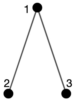
(a) Original graph ${\mathcal{G}}$

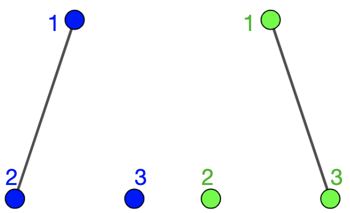
(b) Subgraphs ${\mathcal{G}}^{1}$ and ${\mathcal{G}}^{2}$

Figure 1: Graph ${\mathcal{G}}$ of the computational network with three nodes and subgraphs ${\mathcal{G}}^{1}$ (in blue), ${\mathcal{G}}^{2}$ (in green)

$${\color[rgb]{0,0,1}{{\bf L}({\mathcal{G}}^{1})=\begin{bmatrix}[r]&1&\text{-}1&0\\ &\text{-}1&1&0\\ &0&0&0\\ \end{bmatrix}}},\quad{\color[rgb]{0.3,0.7,0.2}{{\bf L}({\mathcal{G}}^{2})=\begin{bmatrix}[r]&1&0&\text{-}1\\ &0&0&0\\ &\text{-}1&0&1\\ \end{bmatrix}}}$$

According to (3) ${\bf W}$ has the following form:

$${\bf W} ={\color[rgb]{0,0,1}{{\bf L}({\mathcal{G}}^{1})}}\otimes{\bf e}_{1}{\bf e}_{1}^{\top}+{\color[rgb]{0.3,0.7,0.2}{{\bf L}({\mathcal{G}}^{2})}}\otimes{\bf e}_{2}{\bf e}_{2}^{\top}$$

$$={\color[rgb]{0,0,1}{\begin{bmatrix}[r]&1&\text{-}1&0\\ &\text{-}1&1&0\\ &0&0&0\\ \end{bmatrix}}}\otimes\begin{bmatrix}[r]&1&0\\ &0&0\end{bmatrix}+{\color[rgb]{0.3,0.7,0.2}{\begin{bmatrix}[r]&1&0&\text{-}1\\ &0&0&0\\ &\text{-}1&0&1\\ \end{bmatrix}}}\otimes\begin{bmatrix}[r]&0&0\\ &0&1\end{bmatrix}$$

$$=\begin{bmatrix}[r]&{\color[rgb]{0,0,1}{1}}&0&{\color[rgb]{0,0,1}{\text{-}1}}&0&{\color[rgb]{0,0,1}{0}}&0\\ &0&{\color[rgb]{0.3,0.7,0.2}{1}}&0&{\color[rgb]{0.3,0.7,0.2}{0}}&0&{\color[rgb]{0.3,0.7,0.2}{\text{-}1}}\\ &{\color[rgb]{0,0,1}{\text{-}1}}&0&{\color[rgb]{0,0,1}{1}}&0&{\color[rgb]{0,0,1}{0}}&0\\ &0&{\color[rgb]{0.3,0.7,0.2}{0}}&0&{\color[rgb]{0.3,0.7,0.2}{0}}&0&{\color[rgb]{0.3,0.7,0.2}{0}}\\ &{\color[rgb]{0,0,1}{0}}&0&{\color[rgb]{0,0,1}{0}}&0&{\color[rgb]{0,0,1}{0}}&0\\ &0&{\color[rgb]{0.3,0.7,0.2}{\text{-}1}}&0&{\color[rgb]{0.3,0.7,0.2}{0}}&0&{\color[rgb]{0.3,0.7,0.2}{1}}\\ \end{bmatrix}$$

On the other hand, the Laplacian of the original network ${\mathcal{G}}$ (not taking into account the different variables) writes as

$${\bf L}({\mathcal{G}})=\begin{bmatrix}[r]&2&\text{-}1&\text{-}1\\ &\text{-}1&1&0\\ &\text{-}1&0&1\\ \end{bmatrix}.$$

Note, that the condition number of ${\bf W}$ is better as compared to the one of ${\bf L}({\mathcal{G}})$: we have $\chi({\bf W})=1$ and $\chi({\bf L}({\mathcal{G}}))=3$.

2.3 Spectrum of ${\bf W}$

In this section, we analyze the spectrum of the novel communication matrix ${\bf W}$.

Lemma 2.2

For matrix ${\bf W}$ defined in (3) we have ${\bf\Lambda}({\bf W})=\bigcup\limits_{\ell=1}^{n}{\bf\Lambda}({\bf L}({\mathcal{G}}^{\ell}))$.

Firstly, let ${\bf W}{\bf x}=\lambda{\bf x}$ for some ${\bf x}\neq 0$ and $\lambda\in\mathbb{C}$. By definition of ${\bf W}$, we have ${\bf L}({\mathcal{G}}^{\ell}){\bf x}^{\ell}=\lambda{\bf x}^{\ell}$ for $\ell=1,\ldots,n$. Since ${\bf x}\neq 0$, there exists $\ell$ such that ${\bf x}^{\ell}\neq 0$, and therefore $\lambda\in\bigcup\limits_{\ell=1}^{n}{\bf\Lambda}({\bf L}({\mathcal{G}}^{\ell}))$.

Secondly, let ${\bf L}({\mathcal{G}}^{\ell}){\bf x}^{\ell}=\lambda{\bf x}^{\ell}$ for some $\ell=1,\ldots,n$. Setting ${\bf x}={\bf x}^{\ell}\otimes{{\bf e}_{n}^{(\ell)}}$ we obtain

$${\bf W}{\bf x} =\sum_{j=1}^{n}({\bf L}({\mathcal{G}}^{\ell})\otimes{\bf e}_{n}^{(j)}{\bf e}_{n}^{(j)\top})({\bf x}^{\ell}\otimes{{\bf e}_{n}^{(\ell)}})$$

$$=({\bf L}({\mathcal{G}}^{\ell}){\bf x}^{\ell})\otimes{{\bf e}_{n}^{(\ell)}}=\lambda({\bf x}^{\ell}\otimes{{\bf e}_{n}^{(\ell)}})=\lambda{\bf x}$$

i.e. $\lambda\in{\bf\Lambda}({\bf W})$. As a result, ${\bf\Lambda}({\bf W})\subseteq\bigcup\limits_{\ell=1}^{n}{\bf\Lambda}({\bf L}({\mathcal{G}}^{\ell}))$ and $\bigcup\limits_{\ell=1}^{n}{\bf\Lambda}({\bf L}({\mathcal{G}}^{\ell}))\subseteq{\bf\Lambda}({\bf W})$, therefore, $\bigcup\limits_{\ell=1}^{n}{\bf\Lambda}({\bf L}({\mathcal{G}}^{\ell}))={\bf\Lambda}({\bf W})$.

It immediately follows from Lemma 2.2 that $\displaystyle\lambda_{\max}({\bf W})=\max_{1\leq\ell\leq n}\lambda_{\max}({\bf L}({\mathcal{G}}^{\ell}))$ and $\displaystyle\lambda_{\min}^{+}({\bf W})=\min_{1\leq\ell\leq n}\lambda_{\min}^{+}({\bf L}({\mathcal{G}}^{\ell}))$. Thus, we have

$$\chi({\bf W})=\frac{\underset{1\leq\ell\leq n}{\max}\lambda_{\max}({\bf L}({\mathcal{G}}^{\ell}))}{\underset{1\leq\ell\leq n}{\min}\lambda_{\min}^{+}({\bf L}({\mathcal{G}}^{\ell}))}.$$ (5)

Concerning the example in Figure 1, we have $\lambda_{\max}({\color[rgb]{0,0,1}{{\bf L}({\mathcal{G}}^{1})}})=\lambda_{\min}^{+}({\color[rgb]{0,0,1}{{\bf L}({\mathcal{G}}^{1})}})=1$, $\lambda_{\max}({\color[rgb]{0.3,0.7,0.2}{{\bf L}({\mathcal{G}}^{2})}})=\lambda_{\min}^{+}({\color[rgb]{0.3,0.7,0.2}{{\bf L}({\mathcal{G}}^{2})}})=1$ and therefore $\chi({\bf W})=1$.

Remark 2.3

We can determine ${\bf L}({\mathcal{G}})$ up to a positive multiplicative constant. Since that we can consider $\lambda_{\max}({\bf L}({\mathcal{G}}^{\ell}))=1$ for all $l=1,...,n$ without loss of generality. For that we need some preprocessing to estimate $\left\{\lambda_{\max}({\bf L}({\mathcal{G}}^{\ell}))\right\}_{l=1}^{n}$ by using Power method (see Golub and Van Loan (2013)) that could be done in a distributed manner. We also note that $\chi({\bf W})$ from (5) can be bounded from below by the largest diameter of graphs ${\mathcal{G}}^{\ell}$, $l=1,...,n$. Moreover, for many important classes of graphs this lower bound is tight up to a $\ln n$ factor Scaman et al. (2017).

3 Illustrative example: cycle of cliques

We illustrate the effect of using matrix ${\bf W}$ defined in (3) on a synthetic example. Our test case is a computing network with a two-level hierarchical structure. In the lower layer we have a clique (i.e. a fully connected graph) with $k\geq 2$ nodes. Each node in a clique is supposed to share a local variable with its neighbors. In the upper level $n$ cliques communicate through undirected cyclic topology: every clique has a “negotiator”, i.e. a node that has links with similar neighboring nodes (first node of every clique w.l.o.g.). We denote our graph ${\mathcal{G}}_{RC}$.

For every clique, we consider its union with two adjacent nodes and call such subgraph a ”crown”, see Figure 2(b). Overall, we have $n$ ”crowns” $\tilde{\mathcal{G}}^{\ell}$, $\ell=1,\ldots,n$, each corresponding to one of the $n$ variables, i.e., each function $\tilde{f}_{i}$ held by a vertex $i$ of $\tilde{\mathcal{G}}^{\ell}$ depends on $x^{\ell}$. Further, if a node $i$ lies in the intersection of two ”crowns”, its part $\tilde{f}_{i}$ of the objective depends also on the variables corresponding to each of the neighboring ”crowns”. All ”crowns” $\tilde{\mathcal{G}}^{\ell}$ are isomorphic and further denote the ”crown” graph as ${\mathcal{G}}_{cr}$.

Consider an example of graph ${\mathcal{G}}_{RC}$ with $n=3$ given in Figure 2(a) and enumerate the vertices of the top ”crown” as shown in Figure 2(b). Here, the lower level of hierarchy are the fully connected cliques, depicted in black. The upper level of communication is an undirected ring (in red). The “crowns” can be treated as the cliques supplemented by two extra vertices and corresponding edges. Then the functions $\tilde{f}_{4},\tilde{f}_{5},\tilde{f}_{6}$ depend only on the variable $x^{1}$ since the corresponding nodes belong only to the top ”crown”. On the other hand, each of the nodes 1, 2, 3 lies in the intersection of all 3 crowns and therefore functions $\tilde{f}_{1},\tilde{f}_{2},\tilde{f}_{3}$ depend on $x^{1},x^{2},x^{3}$.

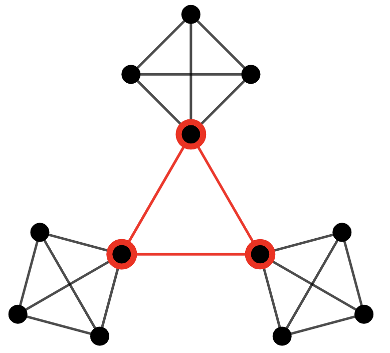
(a) Graph ${\mathcal{G}}_{RC}$ with $n=3$ cliques of size $k=4$

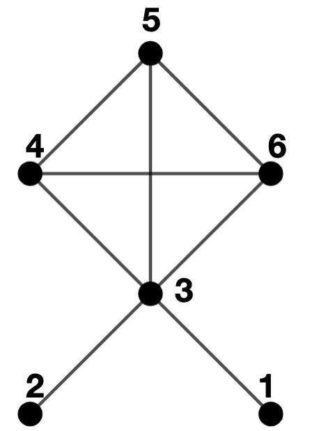
(b) Subgraph ${\mathcal{G}}_{cr}$ corresponding to
variable $x^{1}$

Figure 2: Hierarchical graph with cliques and its ”crown” subgraph

In this section, we illustrate that matrix ${\bf W}$ defined in (3) has a better condition number than the Laplacian ${\bf L}({\mathcal{G}}_{RC})$.

Theorem 3.1

For the hierarchical ring-clique graph it holds

$$\chi({\bf W})=\Theta(k),~{}\chi({\bf L}({\mathcal{G}}_{RC}))=\Theta(n^{2}k^{2}).$$

We prove Theorem 3.1 in a sequence of Lemmas 3.4, 3.5, 3.6, 3.7 presented below in this section. The full proofs of the Lemmas are presented in Appendix. Theorem 3.1 illustrates the flexibility and efficiency of our approach compared to standard approaches that do not take into account the partitioned structure of problem (1). Substituting matrix ${\bf W}$ instead of ${\bf L}({\mathcal{G}}_{RC})$ allows to enhance the convergence rate of distributed algorithms. In the following corollary, we illustrate this speedup on state-of-the-art primal and dual optimization methods.

Corollary 3.2

Let all the functions $f_{i}$, be $L$-smooth, $\mu$ strongly-convex and stored at the nodes of ${\mathcal{G}}_{RC}$. Consider two algorithms: dual MSDA Scaman et al. (2017) and primal OPAPC Kovalev et al. (2020). If we use ${\bf L}({\mathcal{G}}_{RC})$, each of these methods has communication complexity $O\left(\sqrt{\frac{L}{\mu}}nk\ln\frac{1}{\varepsilon}\right)$; the communication complexity becomes $O\left(\sqrt{\frac{L}{\mu}}\sqrt{k}\ln\frac{1}{\varepsilon}\right)$ if we use ${\bf W}$, where $\varepsilon$ is the accuracy.

Remark 3.3

Obviously, in general case there may be examples of graphs where our approach does not provide significant improvement in terms of condition numbers of the corresponding Laplacian matrices. However, the essential feature of partitioned representation of the state vector with sharing of the necessary states only makes this formulation of the distributed optimization problem attractive in terms of more sparse communication topology and reduced information exchange (as compared to (4)). It also corresponds to the preservation of the privacy of the data of interacting groups of nodes.

We first estimate $\chi({\bf W})$. From Lemma 2.2 it follows that ${\bf\Lambda}({\bf W})={\bf\Lambda}({\bf L}({\mathcal{G}}_{cr}))$, where ${\mathcal{G}}_{cr}$ denotes the ”crown” graph. To estimate the asymptotics of the condition number of ”crown” graph, i.e., the condition number of its Laplacian, we use a technique described in Pozrikidis (2014).

Lemma 3.4

The condition number of crown-graph has asymptotics $\chi({\bf L}({\mathcal{G}}_{cr}))=\Theta(k)$, where $k$ is the clique size.

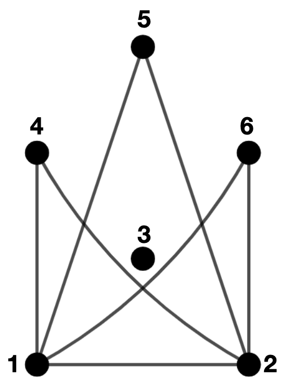
Figure 3: Complement of ${\mathcal{G}}_{rc}$

Firstly, to find the eigenvalues of ${\bf L}({\mathcal{G}}_{cr})$, we find the eigenvalues of ${\bf L}(\bar{{\mathcal{G}}}_{cr})$, where $\bar{{\mathcal{G}}}_{cr}$ is the complement of ${\mathcal{G}}_{cr}$.

The complement has one isolated vertex (node 3 in Figure 3). We denote the Laplacian of the connected part of $\bar{\mathcal{G}}_{cr}$ (i.e. graph in Figure 3 with vertices $\left\{1,2,4,5,6\right\}$) as ${\bf L}^{\prime}(\bar{{\mathcal{G}}}_{cr})$.

$${\bf L}^{\prime} (\bar{\mathcal{G}}_{cr})=\operatorname{diag}(k+2,k+2,2,\ldots,2)$$

$$-{\mathbf{1}}_{k+1}({\bf e}_{k+1}^{(1)}+{\bf e}_{k+1}^{(2)})^{\top}-({\bf e}_{k+1}^{(1)}+{\bf e}_{k+1}^{(2)}){\mathbf{1}}_{k+1}^{\top}$$

Eigenvalues $\lambda^{\prime}$ of ${\bf L}^{\prime}(\bar{\mathcal{G}}_{cr})$ are defined through the equation

$$\text{det}\left({\bf L}^{\prime}\left(\bar{\mathcal{G}}_{cr}\right)-\lambda^{\prime}{\bf I}_{k+1}\right)=0$$

which, via linear conversions (see Appendix A for details), leads us to the equation

$$\lambda^{\prime}(\lambda^{\prime}-k-1)^{2}(\lambda^{\prime}-2)^{k-2}=0.$$

Thus, the eigenvalues of ${\bf L}^{\prime}\left(\bar{{\mathcal{G}}}_{cr}\right)$ have the form $\lambda_{1}^{\prime}=0,~{}\lambda_{2}^{\prime}=\lambda_{3}^{\prime}=k+1,~{}\lambda_{4}^{\prime}=\ldots=\lambda_{k+1}^{\prime}=2$. Using Eq. $2.2.22$ from Pozrikidis (2014), we obtain the eigenvalues of ${\bf L}\left({\mathcal{G}}_{cr}\right)$ to be $\lambda_{1}=0,~{}\lambda_{2}=k+2,~{}\lambda_{3}=\lambda_{4}=1,~{}\lambda_{5}=\ldots=\lambda_{k+2}=k$. Thus, we have $\chi({\bf L}({\mathcal{G}}_{cr}))=(k+2)/1=\Theta(k)$.

Applying Lemma 2.2 we obtain $\chi({\bf W})=\chi({\bf L}({\mathcal{G}}_{cr}))=\Theta(k)$.

Our next goal is to estimate $\chi({\bf L}({\color[rgb]{0,0,0}{\mathcal{G}}_{RC}}))$ and show that it is worse than $\chi({\bf W})$. To compute $\chi({\bf L}({\mathcal{G}}_{RC}))$, we decompose ${\bf L}({\mathcal{G}}_{RC})$ into Laplacians of a $k$-clique ${\mathcal{G}}_{C}$ and a ring graph ${\mathcal{G}}_{R}$ that has $n$ nodes. We also introduce matrix ${\bf B}={\bf e}_{k}^{(1)}{\bf e}_{k}^{(1)\top}$ that allows us to write ${\bf L}({\mathcal{G}}_{RC})$ in the following form.

$$\bf{{\bf L}({\mathcal{G}}_{RC})}={\bf I}_{n}\otimes{\bf L}({\mathcal{G}}_{C})+{\bf L}({\mathcal{G}}_{R})\otimes{\bf B}$$ (6)

Let $\left\{\lambda_{i}\right\}_{i=1}^{n}$ be the eigenvalues of ${\mathcal{G}}_{R}$. To obtain the eigenvalues of ${\bf L}({\mathcal{G}}_{RC})$, we diagonalize it and decompose its spectrum. The result is formulated in the following Lemma.

Lemma 3.5

${\bf\Lambda}({\bf L}({\mathcal{G}}_{RC}))=\bigcup\limits_{i=1}^{n}{\bf\Lambda}({\bf L}({\mathcal{G}}_{C})+\lambda_{i}{\bf B})$.

Let ${\bf L}({\mathcal{G}}_{R})={\bf S}\Psi{\bf S}^{\top}$, where $\Psi=\operatorname{diag}\left(\lambda_{1},\lambda_{2},\ldots,\lambda_{n}\right)$ is a diagonal matrix with eigenvalues of ${\bf L}({\mathcal{G}}_{R})$ and ${\bf S}{\bf S}^{\top}={\bf I}_{n}$. We define

$$\widehat{\bf L}=\left({\bf S}\otimes{\bf I}_{k}\right)^{\top}{\bf L}({\mathcal{G}}_{RC})\left({\bf S}\otimes{\bf I}_{k}\right)={\bf I}_{n}\otimes{\bf L}({\mathcal{G}}_{C})+\Psi\otimes{\bf B}.$$

We have ${\bf\Lambda}(\widehat{\bf L})={\bf\Lambda}({\bf L}({\mathcal{G}}_{RC}))$. Indeed, let ${\bf x}$ be an eigenvector of ${\bf L}({\mathcal{G}}_{RC})$ such that ${\bf L}({\mathcal{G}}_{RC}){\bf x}=\theta{\bf x}$. Then

$$\widehat{\bf L}\cdot(({\bf S}\otimes{\bf I}_{k})^{\top}{\bf x})=\theta\cdot(({\bf S}\otimes{\bf I}_{k})^{\top}{\bf x}),$$

i.e., $({\bf S}\otimes{\bf I}_{k})^{\top}{\bf x}$ is an eigenvector of $\widehat{\bf L}$.

Further, for any eigenvalue $\theta$ of $\widehat{\bf L}$, we have

$$\widehat{\bf L}\begin{bmatrix}x_{1}\\ \vdots\\ x_{n}\end{bmatrix}=\begin{bmatrix}\left({\bf L}({\mathcal{G}}_{C})+\lambda_{1}{\bf B}\right)x_{1}\\ \vdots\\ \left({\bf L}({\mathcal{G}}_{C})+\lambda_{n}{\bf B}\right)x_{n}\end{bmatrix}=\theta\begin{bmatrix}x_{1}\\ \vdots\\ x_{n}\end{bmatrix},$$

i.e., $({\bf L}({\mathcal{G}}_{C})+\lambda_{i}{\bf B})x_{i}=\theta x_{i}$ for $i=1,\ldots,n$. Consequently, ${\bf\Lambda}(\widehat{\bf L})=\bigcup\limits_{i=1}^{n}{\bf\Lambda}({\bf L}({\mathcal{G}}_{C})+\lambda_{i}{\bf B})$, which concludes the proof. Due to Lemma 3.5, we only have to find the spectra ${\bf\Lambda}({\bf L}({\mathcal{G}}_{C})+\lambda_{i}{\bf B})$ for $i=1,\ldots,n$. This is done using the matrix determinant lemma.

Lemma 3.6

The matrix ${\bf L}({\mathcal{G}}_{C})+\lambda{\bf B}$ has the following eigenvalues.

$$\theta_{1}(\lambda) =\dfrac{k+\lambda+\sqrt{\lambda^{2}+2(k-2)\lambda+k^{2}}}{2},$$ (7a)

$$\theta_{2}(\lambda) =\dfrac{k+\lambda-\sqrt{\lambda^{2}+2(k-2)\lambda+k^{2}}}{2},$$ (7b)

$$\theta_{3}(\lambda) =\ldots=\theta_{n}(\lambda)=k.$$

Let $\theta$ denote some eigenvalue of ${\bf L}({\mathcal{G}}_{C})+\lambda{\bf B}$. Then, ${\bf L}({\mathcal{G}}_{C})+\lambda{\bf B}-\theta{\bf I}_{k}={\bf A}-{\mathbf{1}}_{k}{\mathbf{1}}_{k}^{\top}$, where ${\bf A}=\operatorname{diag}\left(k+\lambda-\theta,k-\theta,\ldots,k-\theta\right)$.

Firstly, note that $\theta=k$ is an eigenvalue of ${\bf L}({\mathcal{G}}_{C})+\lambda{\bf B}$. Secondly, $\theta=k+\lambda$ is an eigenvalue of ${\bf L}({\mathcal{G}}_{C})+\lambda{\bf B}$ if and only if $\lambda=0$ (details can be found in Appendix B).

Further, we assume that $\theta\neq k$ and $\theta\neq k+\lambda$. According to the matrix determinant lemma we have

det $$\left({\bf A}-{\mathbf{1}}_{k}{\mathbf{1}}_{k}^{\top}\right)=\left(1-{\mathbf{1}}^{\top}\cdot{\bf A}^{-1}\cdot{\mathbf{1}}\right)\cdot\text{det}{\bf A}$$

$$=(k-\theta)^{k-2}(\theta-\theta_{1})(\theta-\theta_{2})$$

where $\theta_{1}$ and $\theta_{2}$ are defined in (7). Details can be found in Appendix B. Equation (7) gives explicit formulas for eigenvalues of ${\bf L}({\mathcal{G}}_{RC})$, and it remains to estimate $\lambda_{\max}({\bf L}({\mathcal{G}}_{RC}))$ and $\lambda_{\min}^{+}({\bf L}({\mathcal{G}}_{RC}))$. The eigenvalues of the ring graph ${\mathcal{G}}_{R}$ have the form $\lambda_{i}=2-2\cos\frac{2\pi i}{n}$. Note that $0\leq\lambda_{i}\leq 4$.

For the largest eigenvalue of ${\bf L}({\mathcal{G}}_{RC})$, we have

$$\lambda_{\max}({\bf L}({\mathcal{G}}_{RC}))\leq\frac{k+4+\sqrt{4+2(k-2)\cdot 2+k^{2}}}{2}=\Theta(k).$$

Estimating $\lambda_{\min}^{+}({\bf L}({\mathcal{G}}_{RC}))$ is less straightforward and we need to compute the minimal $\theta_{2}$ defined in (7b) over $\lambda\in\left\{\lambda_{1},\ldots,\lambda_{n}\right\}$.

Lemma 3.7

It holds that $\lambda_{\min}^{+}({\bf L}({\mathcal{G}}_{RC}))=\Theta(\frac{1}{n^{2}k})$.

Firstly, let us show that $\theta_{2}(\lambda)$ defined in (7b) is monotonically increasing by considering its derivative:

$$\frac{d\theta_{2}(\lambda)}{d\lambda}=\dfrac{-k-\lambda+2}{2\sqrt{k^{2}+\lambda^{2}+2(k-2)\lambda}}+\dfrac{1}{2}$$

Since $k\geq 2$ it holds $k+\lambda-2<\sqrt{k^{2}+\lambda^{2}+2(k-2)\lambda}$ and we have $\frac{d\theta_{2}(\lambda)}{d\lambda}>0$. Since $\theta_{2}(0)=0$, the minimal positive eigenvalue of ${\bf L}({\mathcal{G}}_{RC})$ is reached at minimal positive $\lambda$, that is, $\lambda_{\min}^{+}({\mathcal{G}}_{RC})=\theta_{2}(2-2\cos\frac{2\pi}{n})$.

Secondly, we approximate $\theta_{2}(2-2\cos\frac{2\pi}{n})$ using the Taylor series at $n\to\infty$ (see Appendix C for details) and get

$$\theta_{2}\left(2-2\cos\frac{2\pi}{n}\right)=\frac{4\pi^{2}}{n^{2}k}+o\left(\frac{1}{n^{3}}\right).$$

It follows that $\lambda_{\min}^{+}({\mathcal{G}}_{RC})=\Theta(\frac{1}{n^{2}k})$.

4 Conclusion

In this paper, we described a simple and universal framework that allows to work with distributed optimization problems with partitioned structure. The proposed method enables to write communication constraints as affine constraints by using a modified Lagrangian matrix. This reformulation lowers the cost of each communication round and also reduces the communication complexities of distributed optimization algorithms.

Appendix

Let ${\bf A}$ and ${\bf B}$ be quadratic matrices of the same size. Throughout the Appendix, we equivalently write $|{\bf A}|$ and $\det({\bf A})$ for determinant of ${\bf A}$. We also write ${\bf A}\sim{\bf B}$ if ${\bf A}$ is obtained from ${\bf B}$ by adding one column (row) multiplied by a scalar to another column (row). Note that if ${\bf A}\sim{\bf B}$ then $\det({\bf A})=\det({\bf B})$.

Appendix A Proof of Lemma 3.4

Firstly, to find the eigenvalues of ${\bf L}({\mathcal{G}}_{cr})$, we find the eigenvalues of ${\bf L}(\bar{{\mathcal{G}}}_{cr})$, where $\bar{{\mathcal{G}}}_{cr}$ is the complement of ${\mathcal{G}}_{cr}$.

The complement has one isolated vertex (node 3 in Figure 3). We denote the Laplacian of the connected part of $\bar{\mathcal{G}}_{cr}$ (i.e. graph in Figure 3 with vertices $\left\{1,2,4,5,6\right\}$) as ${\bf L}^{\prime}(\bar{{\mathcal{G}}}_{cr})$.

$${\bf L}^{\prime} (\bar{\mathcal{G}}_{cr})=\operatorname{diag}(k+2,k+2,2,\ldots,2)-{\mathbf{1}}_{k+1}({\bf e}_{k+1}^{(1)}+{\bf e}_{k+1}^{(2)})^{\top}-({\bf e}_{k+1}^{(1)}+{\bf e}_{k+1}^{(2)}){\mathbf{1}}_{k+1}^{\top}.$$

Eigenvalues $\lambda^{\prime}$ of ${\bf L}^{\prime}(\bar{\mathcal{G}}_{cr})$ are defined through the equation

$$\text{det}\left({\bf L}^{\prime}\left(\bar{\mathcal{G}}_{cr}\right)-\lambda^{\prime}{\bf I}_{k+1}\right)=0.$$

Now we find the roots of the equation above.

$${\bf L}^{\prime}(\overline{\mathcal{G}}_{cr})-\lambda^{\prime}{\bf I}_{k+1} =\begin{bmatrix}&k-\lambda^{\prime}~{}~{}&-1~{}~{}&-1~{}~{}&\cdots&\cdots&-1\\ &-1~{}~{}&k-\lambda^{\prime}~{}~{}&-1~{}~{}&{\cdots}&{\cdots}&-1\\ &-1~{}~{}&-1~{}~{}&2-\lambda^{\prime}~{}~{}&0&{\cdots}&0\\ &{\vdots}~{}~{}&{\vdots}~{}~{}&0~{}~{}&\ddots&&{\vdots}\\ &{\vdots}~{}~{}&{\vdots}~{}~{}&{\vdots}~{}~{}&&\ddots&0\\ &-1~{}~{}&-1~{}~{}&0~{}~{}&{\cdots}&0&2-\lambda^{\prime}\\ \end{bmatrix}\sim\begin{bmatrix}&k-\lambda^{\prime}+1~{}~{}&-1~{}~{}&-1~{}~{}&\cdots&\cdots&-1\\ &\lambda^{\prime}-k-1~{}~{}&k-\lambda^{\prime}~{}~{}&-1~{}~{}&{\cdots}&{\cdots}&-1\\ &0~{}~{}&-1~{}~{}&2-\lambda^{\prime}~{}~{}&0&{\cdots}&0\\ &{\vdots}~{}~{}&{\vdots}~{}~{}&0~{}~{}&\ddots&&{\vdots}\\ &{\vdots}~{}~{}&{\vdots}~{}~{}&{\vdots}~{}~{}&&\ddots&0\\ &0~{}~{}&-1~{}~{}&0~{}~{}&{\cdots}&0&2-\lambda^{\prime}\\ \end{bmatrix}$$

$$\sim\begin{bmatrix}&2k-2\lambda^{\prime}+2~{}~{}&\lambda^{\prime}-k-1~{}~{}&0~{}~{}&\cdots&\cdots&0\\ &\lambda^{\prime}-k-1~{}~{}&k-\lambda^{\prime}~{}~{}&-1~{}~{}&{\cdots}&{\cdots}&-1\\ &0~{}~{}&-1~{}~{}&2-\lambda^{\prime}~{}~{}&0&{\cdots}&0\\ &{\vdots}~{}~{}&{\vdots}~{}~{}&0~{}~{}&\ddots&&{\vdots}\\ &{\vdots}~{}~{}&{\vdots}~{}~{}&{\vdots}~{}~{}&&\ddots&0\\ &0~{}~{}&-1~{}~{}&0~{}~{}&{\cdots}&0&2-\lambda^{\prime}\\ \end{bmatrix}.$$

Then

$$\text{det}\begin{bmatrix}&k-\lambda^{\prime}~{}~{}&-1~{}~{}&-1~{}~{}&\cdots&\cdots&-1\\ &-1~{}~{}&k-\lambda^{\prime}~{}~{}&-1~{}~{}&{\cdots}&{\cdots}&-1\\ &-1~{}~{}&-1~{}~{}&2-\lambda^{\prime}~{}~{}&0&{\cdots}&0\\ &{\vdots}~{}~{}&{\vdots}~{}~{}&0~{}~{}&\ddots&&{\vdots}\\ &{\vdots}~{}~{}&{\vdots}~{}~{}&{\vdots}~{}~{}&&\ddots&0\\ &-1~{}~{}&-1~{}~{}&0~{}~{}&{\cdots}&0&2-\lambda^{\prime}\\ \end{bmatrix}$$

$$\qquad=(2k-2\lambda^{\prime}+2)\begin{vmatrix}&k-\lambda^{\prime}~{}~{}&-1~{}~{}&{\cdots}&{\cdots}&-1\\ &-1~{}~{}&2-\lambda^{\prime}~{}~{}&0&{\cdots}&0\\ &{\vdots}~{}~{}&0~{}~{}&\ddots&&{\vdots}\\ &{\vdots}~{}~{}&{\vdots}~{}~{}&&\ddots&0\\ &-1~{}~{}&0~{}~{}&{\cdots}&0&2-\lambda^{\prime}\\ \end{vmatrix}-(\lambda^{\prime}-k-1)\begin{vmatrix}&\lambda^{\prime}-k-1~{}~{}&-1~{}~{}&{\cdots}&{\cdots}&-1\\ &0~{}~{}&2-\lambda^{\prime}~{}~{}&0&{\cdots}&0\\ &{\vdots}~{}~{}&0~{}~{}&\ddots&&{\vdots}\\ &{\vdots}~{}~{}&{\vdots}~{}~{}&&\ddots&0\\ &0~{}~{}&0~{}~{}&{\cdots}&0&2-\lambda^{\prime}\\ \end{vmatrix}.$$

For the second term we have

$$\begin{vmatrix}&\lambda^{\prime}-k-1~{}~{}&-1~{}~{}&{\cdots}&{\cdots}&-1\\ &0~{}~{}&2-\lambda^{\prime}~{}~{}&0&{\cdots}&0\\ &{\vdots}~{}~{}&0~{}~{}&\ddots&&{\vdots}\\ &{\vdots}~{}~{}&{\vdots}~{}~{}&&\ddots&0\\ &0~{}~{}&0~{}~{}&{\cdots}&0&2-\lambda^{\prime}\\ \end{vmatrix}=(\lambda^{\prime}-k-1)(2-\lambda^{\prime})^{k-1}.$$

For the first term we have

$$\begin{vmatrix}&k-\lambda^{\prime}~{}~{}&-1~{}~{}&{\cdots}&{\cdots}&-1\\ &-1~{}~{}&2-\lambda^{\prime}~{}~{}&0&{\cdots}&0\\ &{\vdots}~{}~{}&0~{}~{}&\ddots&&{\vdots}\\ &{\vdots}~{}~{}&{\vdots}~{}~{}&&\ddots&0\\ &-1~{}~{}&0~{}~{}&{\cdots}&0&2-\lambda^{\prime}\\ \end{vmatrix}$$

$$\qquad=(k-\lambda^{\prime})(2-\lambda^{\prime})^{k\text{-}1}-(-1)\cdot\begin{vmatrix}&-1~{}~{}&0~{}~{}&\cdots&0\\ &-1~{}~{}&2-\lambda^{\prime}~{}~{}&\cdots&0\\ &\vdots~{}~{}&\vdots~{}~{}&\ddots&\vdots\\ &-1~{}~{}&0~{}~{}&\cdots&2-\lambda^{\prime}\\ \end{vmatrix}+(-1)\cdot\begin{vmatrix}&-1~{}~{}&2-\lambda^{\prime}~{}~{}&0&\cdots&0\\ &-1~{}~{}&0~{}~{}&0&\cdots&0\\ &-1~{}~{}&0~{}~{}&2-\lambda^{\prime}&&\vdots\\ &\vdots~{}~{}&\vdots~{}~{}&&\ddots&0\\ &-1~{}~{}&0~{}~{}&\cdots&0&2-\lambda^{\prime}\\ \end{vmatrix}-(-1)\cdot\ldots$$

$$\qquad=(k-\lambda^{\prime})(2-\lambda^{\prime})^{k-1}-(k-1)\cdot(2-\lambda^{\prime})^{k-2}.$$

Consequently,

$$\det({\bf L}^{\prime}(\overline{\mathcal{G}}_{cr})-\lambda^{\prime}{\bf I}_{k+1}) =(2k-2\lambda^{\prime}+2)\left((k-\lambda^{\prime})(2-\lambda^{\prime})^{k-1}-(k-1)(2-\lambda^{\prime})^{k-2}\right)-(\lambda^{\prime}-k-1)^{2}(2-\lambda^{\prime})^{k-1}$$

$$=\left[(k-\lambda^{\prime}+1)(2-\lambda^{\prime})^{k-2}\right]\cdot\left[2(k-\lambda^{\prime})(2-\lambda^{\prime})-2(k-1)-(k-\lambda^{\prime}-1)(2-\lambda^{\prime})\right]$$

$$=(k-\lambda^{\prime}+1)(2-\lambda^{\prime})^{k-2}\cdot[\lambda^{\prime}(\lambda^{\prime}-k-1)].$$

which leads us to the equation

$$\lambda^{\prime}(\lambda^{\prime}-k-1)^{2}(\lambda^{\prime}-2)^{k-2}=0.$$

Thus, the eigenvalues of ${\bf L}^{\prime}\left(\bar{{\mathcal{G}}}_{cr}\right)$ have the form $\lambda_{1}^{\prime}=0,~{}\lambda_{2}^{\prime}=\lambda_{3}^{\prime}=k+1,~{}\lambda_{4}^{\prime}=\ldots=\lambda_{k+1}^{\prime}=2$. Using Eq. $2.2.22$ from Pozrikidis (2014), we obtain the eigenvalues of ${\bf L}\left({\mathcal{G}}_{cr}\right)$ to be $\lambda_{1}=0,~{}\lambda_{2}=k+2,~{}\lambda_{3}=\lambda_{4}=1,~{}\lambda_{5}=\ldots=\lambda_{k+2}=k$. Thus, we have $\chi({\bf L}({\mathcal{G}}_{cr}))=(k+2)/1=\Theta(k)$.

Appendix B Proof of Lemma 3.6

Let $\theta$ denote some eigenvalue of ${\bf L}({\mathcal{G}}_{C})+\lambda{\bf B}$. Then, ${\bf L}({\mathcal{G}}_{C})+\lambda{\bf B}-\theta{\bf I}_{k}={\bf A}-{\mathbf{1}}_{k}{\mathbf{1}}_{k}^{\top}$, where

$${\bf A}=\operatorname{diag}\left(k+\lambda-\theta,k-\theta,\ldots,k-\theta\right)=\begin{bmatrix}&k+\lambda-\theta&0&{\cdots}&{\cdots}&0\\ &0&k-\theta&0&{\cdots}&0\\ &{\vdots}&0&\ddots&\ddots&{\vdots}\\ &{\vdots}&{\vdots}&\ddots&\ddots&0\\ &0&0&{\cdots}&0&k-\theta\\ \end{bmatrix}$$

Firstly, note that $\theta=k$ is an eigenvalue of ${\bf L}({\mathcal{G}}_{C})+\lambda{\bf B}$.

Secondly, note that $\theta=k+\lambda$ is an eigenvalue of ${\bf L}({\mathcal{G}}_{C})+\lambda{\bf B}$ if and only if $\lambda=0$. Indeed, for $\theta=k+\lambda$ it holds

$${\bf A}-{\mathbf{1}}_{k}{\mathbf{1}}_{k}^{\top} =\begin{bmatrix}-1~{}~{}&-1~{}~{}&-1~{}~{}&\ldots~{}~{}&-1\\ -1~{}~{}&-\lambda-1~{}~{}&-1~{}~{}&\ldots~{}~{}&-1\\ -1~{}~{}&-1~{}~{}&-\lambda-1~{}~{}&\ldots~{}~{}&-1\\ \vdots~{}~{}&\vdots~{}~{}&\vdots&\ddots~{}~{}&~{}~{}\vdots\\ -1~{}~{}&-1~{}~{}&-1~{}~{}&\ldots~{}~{}&-\lambda-1\end{bmatrix}\sim\begin{bmatrix}-1~{}~{}&-1~{}~{}&-1~{}~{}&\ldots~{}~{}&-1\\ ~{}~{}0~{}~{}&-\lambda~{}~{}&~{}~{}0~{}~{}&\ldots~{}~{}&~{}~{}0\\ -1~{}~{}&-1~{}~{}&-\lambda-1~{}~{}&\ldots~{}~{}&-1\\ \vdots~{}~{}&\vdots~{}~{}&\vdots&\ddots~{}~{}&~{}~{}\vdots\\ -1~{}~{}&-1~{}~{}&-1~{}~{}&\ldots~{}~{}&-\lambda-1\end{bmatrix}$$

$$\sim\begin{bmatrix}-1~{}~{}&0~{}~{}&-1~{}~{}&\ldots~{}~{}&-1\\ ~{}~{}0~{}~{}&-\lambda~{}~{}&~{}~{}0~{}~{}&\ldots~{}~{}&~{}~{}0\\ -1~{}~{}&0~{}~{}&-\lambda-1~{}~{}&\ldots~{}~{}&-1\\ \vdots~{}~{}&\vdots~{}~{}&\vdots&\ddots~{}~{}&~{}~{}\vdots\\ -1~{}~{}&0~{}~{}&-1~{}~{}&\ldots~{}~{}&-\lambda-1\end{bmatrix}\sim\ldots\sim\begin{bmatrix}-1~{}~{}&~{}~{}0~{}~{}&~{}~{}0~{}~{}&\ldots~{}~{}&~{}~{}0\\ ~{}~{}0~{}~{}&-\lambda~{}~{}&~{}~{}0~{}~{}&\ldots~{}~{}&~{}~{}0\\ ~{}~{}0~{}~{}&~{}~{}0~{}~{}&-\lambda~{}~{}&\ldots~{}~{}&~{}~{}0\\ \vdots~{}~{}&\vdots~{}~{}&\vdots&\ddots~{}~{}&~{}~{}\vdots\\ ~{}~{}0~{}~{}&~{}~{}0~{}~{}&~{}~{}0~{}~{}&\ldots~{}~{}&-\lambda\end{bmatrix}.$$

Therefore, $\det({\bf A}-{\mathbf{1}}_{k}{\mathbf{1}}_{k}^{\top})=(-1)^{k}\lambda^{k-1}$ and $\det({\bf A}-{\mathbf{1}}_{k}{\mathbf{1}}_{k}^{\top})$ if and only if $\lambda=0$. We conclude that either $\theta=k+\lambda=k$ (when $\lambda=0$) or $\theta=k+\lambda$ is not an eigenvalue of ${\bf L}({\mathcal{G}}_{C}+\lambda{\bf B})$ (when $\lambda\neq 0$).

Further, we assume that $\theta\neq k$ and $\theta\neq k+\lambda$.

By definition of ${\bf A}$ we have $\det({\bf A})=(k+\lambda-\theta)(k-\theta)^{k-1}\neq 0$.

According to matrix determinant lemma (see Lemma $1.1$ from Ding and Zhou (2007)):

$$\text{det}\left({\bf A}-{\mathbf{1}}_{k}{\mathbf{1}}_{k}^{\top}\right)=\left(1-{\mathbf{1}}_{k}^{\top}{\bf A}^{-1}{\mathbf{1}}_{k}\right)\cdot\text{det}{\bf A}$$

Since $\theta\neq k$ and $\theta\neq k+\lambda$ we have

$${\bf A}^{-1}=\begin{bmatrix}&\dfrac{1}{k+\lambda-\theta}&0&{\cdots}&{\cdots}&0\\ &0&\dfrac{1}{k-\theta}&0&{\cdots}&0\\ &{\vdots}&0&\ddots&\ddots&{\vdots}\\ &{\vdots}&{\vdots}&\ddots&\ddots&0\\ &0&0&{\cdots}&0&\dfrac{1}{k-\theta}\\ \end{bmatrix}$$

It follows that $1-{\mathbf{1}}_{k}^{\top}{\bf A}^{-1}{\mathbf{1}}_{k}=1-\dfrac{1}{k+\lambda-\theta}-\dfrac{k-1}{k-\theta}$.

$$\text{det}({\bf L}({\mathcal{G}}_{C})+\lambda{\bf B}-\theta{\bf I}_{k}) = \left(1-\dfrac{1}{k+\lambda-\theta}-\dfrac{k-1}{k-\theta}\right)(k+\lambda-\theta)(k-\theta)^{k-1}$$

$$=(k+\lambda-\theta)(k-\theta)^{k-1}-(k-\theta)^{k-1}-(k-1)(k+\lambda-\theta)(k-\theta)^{k-2}$$

$$=(k-\theta)^{k-2}\cdot\left((k+\lambda-\theta)\cdot(k-\theta)-(k-\theta)-(k-1)(k+\lambda-\theta)\right)$$

$$=(k-\theta)^{k-2}\left(\theta^{2}+\theta(-k-\lambda)+\lambda\right)$$

$$=(k-\theta)^{k-2}\left(\theta-\theta_{1}\right)\left(\theta-\theta_{2}\right).$$

Here

$$\theta_{1} =\dfrac{k+\lambda+\sqrt{\lambda^{2}+2(k-2)\lambda+k^{2}}}{2},$$

$$\theta_{2} =\dfrac{k+\lambda-\sqrt{\lambda^{2}+2(k-2)\lambda+k^{2}}}{2}.$$

The rest eigenvalues are $\theta_{3}=\ldots=\theta_{k}=k$.

Appendix C Proof of Lemma 3.7

Firstly, let us show that $\theta_{2}(\lambda)$ defined in (7b) is monotonically increasing by considering its derivative:

$$\frac{d\theta_{2}(\lambda)}{d\lambda}=\dfrac{-k-\lambda+2}{2\sqrt{k^{2}+\lambda^{2}+2(k-2)\lambda}}+\dfrac{1}{2}$$

Since $k\geq 2$, it holds $k+\lambda-2<\sqrt{k^{2}+\lambda^{2}+2(k-2)\lambda}$ and we have $\frac{d\theta_{2}(\lambda)}{d\lambda}>0$. Since $\theta_{2}(0)=0$, the minimal positive eigenvalue of ${\bf L}({\mathcal{G}}_{RC})$ is reached at minimal positive $\lambda$, that is, $\lambda_{\min}^{+}({\mathcal{G}}_{RC})=\theta_{2}(2-2\cos\frac{2\pi}{n})$.

Secondly, we approximate $\theta_{2}(2-2\cos\frac{2\pi}{n})$ using the Taylor series at $n\to\infty$.

$$\theta_{2}\left(2-2\cos\frac{2\pi}{n}\right) =\frac{1}{2}\left[k+2\left(\frac{4\pi^{2}}{2n^{2}}+o\left(\frac{1}{n^{3}}\right)\right)-k\left(1+4\frac{k-2}{k^{2}}\cdot\frac{4\pi^{2}}{2n^{2}}+o\left(\frac{1}{n^{3}}\right)+\frac{4}{k^{2}}\left(\frac{4\pi^{2}}{2n^{2}}+o\left(\frac{1}{n^{3}}\right)\right)^{2}\right)^{1/2}\right]$$

$$=\frac{1}{2}\left[k+\frac{4\pi^{2}}{n^{2}}+o\left(\frac{1}{n^{3}}\right)-k\left(1+\frac{4\pi^{2}}{kn^{2}}\left(1-\frac{2}{k}\right)+o\left(\frac{1}{n^{3}}\right)\right)\right]$$

$$=\frac{1}{2}\left[\frac{4\pi^{2}}{n^{2}}-\frac{4\pi^{2}}{n^{2}}+\frac{8\pi^{2}}{kn^{2}}+o\left(\frac{1}{n^{3}}\right)\right]=\frac{4\pi^{2}}{kn^{2}}+o\left(\frac{1}{n^{3}}\right)$$

Therefore, we obtain

$$\lambda_{\text{min}}^{+}({\mathcal{G}}_{RC})\sim\Theta\left(\dfrac{1}{n^{2}k}\right).$$

References

- Borkar and Varaiya (1982) Borkar, V. and Varaiya, P.P. (1982). Asymptotic agreement in distributed estimation. IEEE Transactions on Automatic Control, 27(3), 650–655.
- Bottou (2010) Bottou, L. (2010). Large-scale machine learning with stochastic gradient descent. In Proceedings of COMPSTAT’2010, 177–186. Springer.
- Boyd et al. (2011) Boyd, S., Parikh, N., Chu, E., Peleato, B., and Eckstein, J. (2011). Distributed optimization and statistical learning via the alternating direction method of multipliers. Foundations and Trends® in Machine Learning, 3(1), 1–122.
- Cannelli et al. (2020) Cannelli, L., Facchinei, F., Scutari, G., and Kungurtsev, V. (2020). Asynchronous optimization over graphs: Linear convergence under error bound conditions. IEEE Transactions on Automatic Control, 66(10), 4604–4619.
- Carli and Notarstefano (2013) Carli, R. and Notarstefano, G. (2013). Distributed partition-based optimization via dual decomposition. In 52nd IEEE Conference on Decision and Control, 2979–2984. IEEE.
- DeGroot (1974) DeGroot, M.H. (1974). Reaching a consensus. Journal of the American Statistical Association, 69(345), 118–121.
- Ding and Zhou (2007) Ding, J. and Zhou, A. (2007). Eigenvalues of rank-one updated matrices with some applications. Applied Mathematics Letters, 20(12), 1223–1226.
- Dvinskikh and Gasnikov (2021) Dvinskikh, D. and Gasnikov, A. (2021). Decentralized and parallel primal and dual accelerated methods for stochastic convex programming problems. Journal of Inverse and Ill-posed Problems.
- Erseghe (2012) Erseghe, T. (2012). A distributed and scalable processing method based upon admm. IEEE Signal Processing Letters, 19(9), 563–566.
- Golub and Van Loan (2013) Golub, G.H. and Van Loan, C.F. (2013). Matrix computations. JHU press.
- Gorbunov et al. (2020) Gorbunov, E., Rogozin, A., Beznosikov, A., Dvinskikh, D., and Gasnikov, A. (2020). Recent theoretical advances in decentralized distributed convex optimization. arXiv preprint arXiv:2011.13259.
- Ivanova et al. (2020) Ivanova, A., Dvurechensky, P., Gasnikov, A., and Kamzolov, D. (2020). Composite optimization for the resource allocation problem. Optimization Methods and Software, 0(0), 1–35. 10.1080/10556788.2020.1712599.
- Kekatos and Giannakis (2012) Kekatos, V. and Giannakis, G.B. (2012). Distributed robust power system state estimation. IEEE Transactions on Power Systems, 28(2), 1617–1626.
- Kovalev et al. (2022) Kovalev, D., Beznosikov, A., Sadiev, A., Persiianov, M., Richtárik, P., and Gasnikov, A. (2022). Optimal algorithms for decentralized stochastic variational inequalities. arXiv preprint arXiv:2202.02771.
- Kovalev et al. (2020) Kovalev, D., Salim, A., and Richtárik, P. (2020). Optimal and practical algorithms for smooth and strongly convex decentralized optimization. Advances in Neural Information Processing Systems, 33.
- Kraska et al. (2013) Kraska, T., Talwalkar, A., Duchi, J.C., Griffith, R., Franklin, M.J., and Jordan, M.I. (2013). Mlbase: A distributed machine-learning system. In CIDR, volume 1, 2–1.
- Kroshnin et al. (2019) Kroshnin, A., Tupitsa, N., Dvinskikh, D., Dvurechensky, P., Gasnikov, A., and Uribe, C. (2019). On the complexity of approximating Wasserstein barycenters. In K. Chaudhuri and R. Salakhutdinov (eds.), Proceedings of the 36th International Conference on Machine Learning, volume 97 of PMLR, 3530–3540. PMLR, Long Beach, California, USA.
- Necoara and Clipici (2016) Necoara, I. and Clipici, D. (2016). Parallel random coordinate descent method for composite minimization: Convergence analysis and error bounds. SIAM Journal on Optimization, 26(1), 197–226.
- Nedić et al. (2017) Nedić, A., Olshevsky, A., and Uribe, C.A. (2017). Fast convergence rates for distributed non-Bayesian learning. IEEE Trans. on Autom. Contr., 62(11), 5538–5553.
- Nedić et al. (2009) Nedić, A., Olshevsky, A., Ozdaglar, A., and Tsitsiklis, J.N. (2009). On distributed averaging algorithms and quantization effects. IEEE Transactions on Automatic Control, 54(11), 2506–2517.
- Notarnicola et al. (2017) Notarnicola, I., Carli, R., and Notarstefano, G. (2017). Distributed partitioned big-data optimization via asynchronous dual decomposition. IEEE Transactions on Control of Network Systems, 5(4), 1910–1919.
- Pozrikidis (2014) Pozrikidis, C. (2014). An introduction to grids, graphs, and networks. Oxford University Press.
- Rabbat and Nowak (2004) Rabbat, M. and Nowak, R. (2004). Decentralized source localization and tracking wireless sensor networks. In Proc. of the IEEE Intl. Conf. on Acoustics, Speech, and Signal Processing, volume 3, 921–924.
- Ram et al. (2009) Ram, S.S., Veeravalli, V.V., and Nedic, A. (2009). Distributed non-autonomous power control through distributed convex optimization. In IEEE INFOCOM 2009, 3001–3005. IEEE.
- Rogozin et al. (2021) Rogozin, A., Beznosikov, A., Dvinskikh, D., Kovalev, D., Dvurechensky, P., and Gasnikov, A. (2021). Decentralized distributed optimization for saddle point problems. arXiv preprint arXiv:2102.07758.
- Scaman et al. (2017) Scaman, K., Bach, F., Bubeck, S., Lee, Y.T., and Massoulié, L. (2017). Optimal algorithms for smooth and strongly convex distributed optimization in networks. In D. Precup and Y.W. Teh (eds.), ICML, volume 70 of PMLR, 3027–3036. PMLR.
- Tsitsiklis and Athans (1984) Tsitsiklis, J.N. and Athans, M. (1984). Convergence and asymptotic agreement in distributed decision problems. IEEE Transactions on Automatic Control, 29(1), 42–50.
- Uribe et al. (2018) Uribe, C.A., Dvinskikh, D., Dvurechensky, P., Gasnikov, A., and Nedić, A. (2018). Distributed computation of Wasserstein barycenters over networks. In 2018 IEEE Conference on Decision and Control (CDC), 6544–6549.
- Xiao and Boyd (2006) Xiao, L. and Boyd, S. (2006). Optimal scaling of a gradient method for distributed resource allocation. Journal of Optimization Theory and Applications, 129(3), 469–488.
- Yang et al. (2019) Yang, T., Yi, X., Wu, J., Yuan, Y., Wu, D., Meng, Z., Hong, Y., Wang, H., Lin, Z., and Johansson, K.H. (2019). A survey of distributed optimization. Annual Reviews in Control, 47, 278–305.