Radiative Plateau Inflation with Conformal Invariance:
Dynamical Generation of Electroweak and Seesaw Scales

Abstract

We investigate a scale-invariant $B-L$ scenario where the Standard Model (SM) is supplemented with a dark scalar $\phi$ which has gauge & Yukawa interactions, with the couplings $g_{BL}$ and $y$, respectively, leading to radiative plateau inflation at scale $\phi=M$ in the ultraviolet (UV), while dynamically generating the Electroweak and Seesaw scales á lá Coleman-Weinberg in the infrared (IR). This is particularly achieved by implementing threshold corrections at an energy scale $\mu_{T}$ arising due to the presence of vector-like fermions. We show that implementing the inflationary observables makes the couplings solely dependent on the plateau scale $M$, leaving us with only two independent parameters $M$ and $\mu_{T}$. Within the theoretically consistent parameter space defined by $m_{Z_{BL}}>850~{}\rm GeV$, from the assumption of independent evolution of the dark sector couplings from the SM couplings and $M<5.67~{}M_{P}$ required for the realisation of inflationary plateau-like behaviour of the potential around $\phi=M$, where $M_{P}=2.4\times 10^{18}$ GeV is the reduced Planck mass, we identify the parameter space that is excluded by the current LHC results from the search for the heavy $Z_{BL}$ boson. For typical benchmark points in the viable parameter regions, we estimate the reheating temperature to be $\mathcal{O}(TeV)$ thus consistent with the standard Big Bang Nucleosynthesis (BBN) constraints. For typical benchmark points ($M=5.67,~{}1,~{}0.1~{}M_{P}$) we predict the scales of inflation to be $\mathcal{H}_{inf}=2.79\times 10^{12}$ GeV, $1.53\times 10^{10}$ GeV and $1.53\times 10^{7}$ GeV, respectively.

I Introduction

Grand Unified Theories (GUTs) formed the basis of the original proposal for the cosmic inflation, an accelerated expansion at the beginning of the universe, which can solve the horizon and the flatness problems as well as provide initial seed of density fluctuations to grow into our inhomogeneous universe as we see today Guth (1981); Sato (1981); Kazanas (1980), and later on, inflation was studied in the context of gravity effective theories like the Starobinsky scenario Nariai and Tomita (1971); Starobinsky (1980). Although the former turned out to be unsuccessful, the quantum generation of the primordial fluctuations seeding the large scale structure (LSS) of the Universe was a successful scenario. Irrespective of the origin of inflationary cosmology being of particle physics or not, the quite rapidly increasing data from cosmological precision measurements, particle physics experiments and astrophysical observations lead us to the quest of a coherent picture of the early Universe based on particle physics to begin with.

Although inflation can be achieved by scalar fields, particularly, slow-roll inflation by a single scalar field ($\phi$), simple potentials like quadratic $m^{2}\phi^{2}$ or quartic $\lambda_{\phi}\phi^{4}$ inflation scenarios which predict too large tensor-to-scalar ratio, have been ruled out by the observations of CMB power spectrum Akrami et al. (2020). Possibilities to rescue such models and make them consistent with the observations have been studied extensively in the literature. Whereas a possibility is to introduce non-minimal coupling of the inflaton to gravity ($\xi\phi^{2}\mathcal{R}$) Bezrukov and Shaposhnikov (2008); Libanov et al. (1998); Fakir and Unruh (1990); Futamase and Maeda (1989); Masina (2018); Okada et al. (2010); Linde (1987); Kallosh et al. (1995); Inagaki et al. (2014) to flatten $\lambda_{\phi}\phi^{4}$ potential during inflation, the same purpose can also be achieved through Renormalization Group (RG)-improved $\lambda_{\phi}\phi^{4}$ potential. The quantum corrections generate a plateau shaped potential, whose flatness near the plateau (inflection point) makes the CMB constraints being satisfied. Particularly, employing bosonic and fermionic quantum corrections to achieve inflection-point inflation were studied in Refs. Okada et al. (2017); Choi and Lee (2016a); Allahverdi et al. (2006, 2007); Bueno Sanchez et al. (2007); Baumann et al. (2007, 2008); Badziak and Olechowski (2009); Enqvist et al. (2010); Cerezo and Rosa (2013); Choudhury et al. (2013); Choudhury and Mazumdar (2014); Ballesteros and Tamarit (2016a); Choi and Lee (2016a); Okada and Raut (2017); Okada et al. (2017); Stewart (1997a, b); Drees and Xu (2021). In this set-up giving precise predictions in the CMB as well as long-lived particle searches Okada and Raut (2017); Okada et al. (2019); Okada and Raut (2019); Ballesteros and Tamarit (2016b); Choi and Lee (2016b); Bai and Stolarski (2020); Dimopoulos et al. (2018); Caputo (2019a); Senoguz and Shafi (2008); Enqvist and Karciauskas (2014); Okada et al. (2021, 2021) have been studied. In this paper we will investigate such a particle physics motivated scenario for inflation.

Any fundamental scalar field in quantum field theory (QFT) suffers from what is known as the hierarchy problem, although the Large Hadron Collider (LHC) was able to shed light on the origin of Electroweak Symmetry Breaking (EWSB) confirming the existence of a Brout-Englert-Higgs scalar doublet (commonly known as the Higgs doublet). In the SM, a non-zero vacuum expectation value (vev) of the Higgs doublet originates from a negative mass squared term in the Higgs potential at the tree level, which is the only mass term allowed by the symmetries of the SM. Quantum corrections to the mass of the SM Higgs doublet turn out to be UV sensitive, so that the effective Higgs mass is naturally be of the order of the Planck scale or the cut-off scale for the theory.

An elegant solution to this problem is to assume scale invariance, and that all scales we observe be generated dynamically. One such attractive possibility was proposed long ago by Coleman and Weinberg, where a gauge symmetry breaking is dynamically (radiatively) generated via quantum corrections. However appealing as it may be, this mechanism fails within the Standard Model to generate the Higgs mass (the Electroweak Scale) because of the contributions of W and Z boson loops and from top quark loops. The original Coleman-Weinberg prediction was that the mass of the gauge bosons is greater than that of the Higgs boson, $m_{Z,W}>m_{H}$ Coleman and Weinberg (1973a); Englert et al. (2013). In BSM scenarios, a picture that no scale is fundamental in nature and all mass scales are generated dynamically, has been explored extensively in the literature Adler (1982); Coleman and Weinberg (1973b); Salvio and Strumia (2014); Einhorn and Jones (2015, 2016a, 2016b). In context of non-minimally coupling to gravity, such scenarios provide naturally flat inflaton potentials Khoze (2013); Kannike et al. (2014); Rinaldi et al. (2015); Salvio and Strumia (2014); Kannike et al. (2015a, b); Barrie et al. (2016); Tambalo and Rinaldi (2017) and dark matter candidates Hambye and Strumia (2013a); Karam and Tamvakis (2015); Kannike et al. (2015a, 2016); Karam and Tamvakis (2016); Barman and Ghoshal (2021), and also leads to very strong first-order phase transitions via supercooling in early universe and therefore the possibility of high amplitude detectable gravitational wave (GW) signals mainly due to dominance of thermal corrections in absence of tree-level mass terms Jaeckel et al. (2016); Marzola et al. (2017); Iso et al. (2017); Baldes and Garcia-Cely (2019); Prokopec et al. (2019); Brdar et al. (2019a); Marzo et al. (2019); Ghoshal and Salvio (2020). Scale invariant scenarios have always been seen as direction of model-building for the hierarchy problem in the Standard Model of particle physics Foot et al. (2008); Alexander-Nunneley and Pilaftsis (2010); Englert et al. (2013); Hambye and Strumia (2013a); Farzinnia et al. (2013); Altmannshofer et al. (2015); Holthausen et al. (2013); Salvio and Strumia (2014); Einhorn and Jones (2015); Kannike et al. (2015a); Farzinnia and Kouwn (2016); Kannike et al. (2016). See Refs. Hambye and Strumia (2013b); Antipin et al. (2015); Iso et al. (2009a, b); Iso and Orikasa (2013); Brivio and Trott (2017a); Brdar et al. (2019b) for other studies of conformal invariance and dimensional transmutation of energy scales Salvio (2020); Buoninfante et al. (2019); Frasca et al. (2022b); Frasca and Ghoshal (2021b); Ghoshal et al. (2021b); Frasca and Ghoshal (2020b); Ghoshal (2019b); Ghoshal et al. (2018b).

Sticking to the scale-invariant BSM framework, we consider a $B-L$ extended SM, in which the $B-L$ symmetry is broken by the Coleman-Weinberg mechanism, subsequently triggering the EW symmetry breaking. The $B-L$ extended SM Mohapatra and Marshak (1980); Marshak and Mohapatra (1980); Wetterich (1981); Masiero et al. (1982); Mohapatra and Senjanovic (1983) have been well-studied which accounts for matter-antimatter asymmetry and the origin of the SM neutrino masses via Type-I seesaw mechanism. Now as we go from UV to IR, quantum corrections from the $B-L$ gauge boson drives the running quartic coupling ($\lambda_{\phi}$) of the $B-L$ Higgs ($\phi$) negative in the IR. What happens is that, once the condition $\lambda_{\phi}<0$ is reached, $\phi$ develops a VEV $\phi=v_{BL}/\sqrt{2}$, and the mixing quartic term $-\lambda_{H\phi}|H|^{2}|\phi|^{2}$ with the SM Higgs doublet ($H$) effectively generates a negative mass squared, $-m^{2}|H|^{2}$ with $m^{2}=\frac{1}{2}\lambda_{H\phi}v_{BL}^{2}$, and hence the EW symmetry is broken. Moreover, we consider a possibility that the $B-L$ Higgs is also responsible for the plateau inflation.

However, using the $B-L$ Higgs with conformal invariance as the inflaton for the radiative plateau inflation is highly non-trivial. Let us see in details why. In order for $B-L$ Higgs to drive the successful plateau inflation, the running of $\lambda_{\phi}(\phi)$ should exhibit a minima $\lambda_{\phi}(\phi=M)\sim 0$, which means $\beta_{\lambda_{\phi}}<0$, $\beta_{\lambda_{\phi}}=0$ and $\beta_{\lambda_{\phi}}>0$ for $\phi<M$, $\phi=M$ and $\phi>M$, respectively, around $\phi=M$. On the other hand, the CW mechanism requires $\lambda_{\phi}$ to be positive at high energies and fall to negative values at a low energy ($\phi\sim v_{BL}/\sqrt{2}$). Therefore, in order for the $B-L$ Higgs to play the dual role of the inflaton for the radiative plateau inflation and for breaking the $B-L$ symmetry by CW mechanism, $\beta_{\lambda_{\phi}}$ changes its sign twice from the UV to IR. It is non-trivial to realize such a behaviour of $\beta_{\lambda_{\phi}}$ in gauge theories.

In this paper, we propose a way to realize the dual role of the $B-L$ Higgs field, where threshold corrections from Majorana fermions at some intermediate scale play a crucial role .

Our basic idea the following. At UV, to realize the successful plateau inflation, $\lambda_{\phi}(\phi=M)\sim 0$ and its beta function is symbolically expressed as $\beta_{\lambda_{\phi}}\sim C_{g}g_{BL}^{4}-C_{y}y^{4}\sim 0$, where $C_{g,y}$ are numerical factors, and $y$ is the Yukawa coupling of a fermion with a mass $m_{F}$. Setting $g_{BL}$ and $y$ suitably, we can realize $\beta_{\lambda_{\phi}}(\phi<M)<0$, $\beta_{\lambda_{\phi}}(\phi=M)=0$ and $\beta_{\lambda_{\phi}}(\phi>M)>0$, for generating the radiative plateau potential at $\phi=M$. Moving towards the IR, the fermion decouples at $\phi=m_{F}$, and therefore, for $\phi<m_{F}$, the beta function changes its sign to $\beta_{\lambda_{\phi}}>0$. Moving to low energies further, $\lambda_{\phi}(\phi)$ eventually becomes negative and the $B-L$ symmetry by is broken by the CW mechanism.

The paper is arranged as follows: in section. II we discuss inflation analysis of this work. In subsections II.1, II.2 and II.3, we discuss on the basics of plateau inflation, the model and on obtaining plateau inflation with the model. In section. III we move to the Coleman-Weinberg part of this work. In subsections III.1, III.2, III.3 and III.4, we discuss the basics of Coleman-Weinberg mechanism, difficulty of achieving plateau inflation and Coleman-Weinberg in the same model, way out of this difficulty and theoretical conditions for this analysis to work respectively. We discuss the reheating analysis of this model in section. IV. We discuss the possible searches for ${Z_{B-L}}$ particle and present the parameter space compatible with current experimental results in section.V. In Section.VI, we discuss the main findings of our paper and its implications.

II Inflation

In this section we will describe how to generate the inflationary plateau-like behaviour from $U(1)_{B-L}$ Higgs quartic potential, expanded around an inflection-point, driven purely due to radiative corrections.

II.1 Basics of Inflection-point Inflation

Quickly re-capping the slow-roll parameters of inflationary observables,

$$\epsilon(\phi)=\frac{M_{P}^{2}}{2}\left(\frac{V^{\prime}}{V}\right)^{2},\;\;\eta(\phi)=M_{P}^{2}\left(\frac{V^{\prime\prime}}{V}\right),\;\;\varsigma^{2}{(\phi)}=M_{P}^{4}\frac{V^{\prime}V^{\prime\prime\prime}}{V^{2}},$$ (1)

where we have the reduced Planck mass $M_{P}=M_{Pl}/\sqrt{8\pi}=2.43\times 10^{18}$ GeV, $V$ is the inflaton potential, and the prime denotes its derivative with respect to the inflaton $\phi$.

In this notation, the curvature perturbation $P^{2}_{\mathcal{R}}$ is given by

$$P_{\mathcal{R}}^{2}=\frac{1}{24\pi^{2}}\frac{1}{M_{P}^{4}}\left.\frac{V}{\epsilon}\right|_{k_{0}},$$ (2)

the value of which should be $P_{\mathcal{R}}^{2}=2.189\times 10^{-9}$ from the Planck 2018 results Akrami et al. (2020) at pivot scale $k_{0}=0.05$ Mpc^-1. The number of e-folds is given by,

$$N=\frac{1}{M_{P}^{2}}\int_{\phi_{E}}^{\phi_{I}}\frac{V}{V^{\prime}}d\phi,$$ (3)

where $\phi_{I}$ is the value of inflaton during horizon exit of the scale $k_{0}$, and $\phi_{E}$ is the value of inflaton value when the slow-roll condition is violated, i.e. $\epsilon(\phi_{E})=1$. The slow-roll approximation holds whenever $\epsilon\ll 1$, $|\eta|\ll 1$ , and $\varsigma^{2}\ll 1$.

The inflationary predictions of the scalar and tensor perturbations are given by,

$$n_{s}=1-6\epsilon+2\eta,\;\;r=16\epsilon,\;\;\alpha=16\epsilon\eta-24\epsilon^{2}-2\varsigma^{2},$$ (4)

where $n_{s}$ and $r$ and $\alpha\equiv\frac{\mathrm{d}n_{s}}{dlnk}$ are the scalar spectral index, the tensor-to-scalar ratio and the running of the spectral index, respectively, at $\phi=\phi_{I}$. Planck 2018 results give an upper bound on $r\lesssim 0.067$, bound for the spectral index ($n_{s}$) and the running of spectral index ($\alpha$) to be $0.9691\pm 0.0041$ and $0.0023\pm 0.0063$, respectively Akrami et al. (2020). A combination of Planck with BICEP/Keck 2018 and Baryon Acoustic Oscillations data tightens the upper bound of tensor-to-scalar ratio to $r<0.032$ Tristram et al. (2021).

The inflaton potential for inflection-point inflation, expanding around an inflection point near $\phi=M$ value of the field is given by Okada and Raut (2017):

$$V(\phi)\simeq V_{0}+\sum_{n=1}^{3}\frac{1}{n!}V_{n}(\phi-M)^{n},$$ (5)

where $V_{0}=V(M)$ is constant, $V_{n}\equiv d^{n}V/d\phi^{n}|_{\phi=M}$ are derivatives evaluated at at $\phi=M$, and the inflection-point $\phi=M$ is the field value at the pivot scale $k_{0}=0.05$ Mpc^-1 of the Planck 2018 measurements Akrami et al. (2020). If the values of $V_{1}$ and $V_{2}$ are tiny enough, inflection-point can be realized. re-writing Eqs. (1) in terms of parameters of Eq. (5),

$$\epsilon(M)\simeq\frac{M_{P}^{2}}{2}\Big{(}\frac{V_{1}}{V_{0}}\Big{)}^{2},\;\;\eta(M)\simeq M_{P}^{2}\Big{(}\frac{V_{2}}{V_{0}}\Big{)},\;\;\zeta^{2}{(M)}=M_{P}^{4}\frac{V_{1}V_{3}}{V_{0}^{2}},$$ (6)

where we have used the approximation $V(M)\simeq V_{0}$. Similarly, the power-spectrum $\Delta_{\mathcal{R}}^{2}$ is expressed as

$$P_{\mathcal{R}}^{2}\simeq\frac{1}{12\pi^{2}}\frac{1}{M_{P}^{6}}\frac{V_{0}^{3}}{V_{1}^{2}}.$$ (7)

Using the observational constraint, $P_{\mathcal{R}}^{2}=2.189\times 10^{-9}$, and a fixed $n_{s}$ value, we obtain

$$\frac{V_{1}}{M^{3}} \simeq 1963\left(\frac{M}{M_{P}}\right)^{3}\left(\frac{V_{0}}{M^{4}}\right)^{3/2},$$

$$\frac{V_{2}}{M^{2}} \simeq -1.545\times 10^{-2}\Big{(}\frac{1-n_{s}}{1-0.9691}\Big{)}\Big{(}\frac{M}{M_{P}}\Big{)}^{2}\left(\frac{V_{0}}{M^{4}}\right),$$ (8)

using $V(M)\simeq V_{0}$. For the remainder of the analysis we set $n_{s}=0.9691$ (the central value from the Planck 2018 results Akrami et al. (2020)). Then V₃ becomes

$$\frac{V_{3}}{M}\simeq 6.983\times 10^{-7}\Big{(}\frac{60}{N}\Big{)}^{2}\Big{(}\frac{V_{0}^{1/2}}{MM_{P}}\Big{)}.$$ (9)

Using Eqs. (4), (6), (8) and (9), the tensor-to-scalar ratio ($r$) is given by

$$r=3.082\times 10^{7}\Big{(}\frac{V_{0}}{M_{P}^{4}}\Big{)}.$$ (10)

and, the running of the spectral index ($\alpha$)

$$\alpha\simeq-2\varsigma^{2}(M)=-\;2.741\times 10^{-3}\left(\frac{60}{N}\right)^{2},$$ (11)

It is interesting to note that the running is independent of the $V_{0}$ and $M$ terms in the inflation potential.

This prediction is consistent with the current experimental bound, $\alpha=0.0023\pm 0.0063$ Akrami et al. (2020). Precision measurement of the running of the spectral index in future experiments can reduce the error to $\pm 0.002$ Ade et al. (2019); Aiola et al. (2020). Hence, the predictions can be tested in the future.

II.2 The $B-L$ Extended Model

Field	Group	Coupling
$Z_{BL}~{}~{}~{}~{}$	$U(1)_{B-L}$	$g_{BL}$

Table 1: New gauge sector of the model

Field	Spin	$U(1)_{B-L}$
$~{}~{}~{}~{}\phi~{}~{}~{}~{}$	$~{}~{}~{}~{}0~{}~{}~{}~{}$	$2$
$~{}~{}~{}~{}\psi_{L,R}~{}~{}~{}~{}$	$~{}~{}~{}~{}\frac{1}{2}~{}~{}~{}~{}$	$-1$
$~{}~{}~{}~{}N_{R}^{i}~{}~{}~{}~{}$	$~{}~{}~{}~{}\frac{1}{2}~{}~{}~{}~{}$	$-1$

Table 2: New scalars and fermions in the model.

We start with the minimal extension of the SM model where the SM gauge group is supplemented with a $U(1)_{B-L}$ local symmetry. In this $B-L$ sector, there are two vector-like fermions $\psi_{L}$ and $\psi_{R}$, three right-handed neutrinos $N_{R}^{i}$, as well as the complex scalar field $\phi$. Tables 1 and 2 show all the details about the gauge sector and the new scalars and fermions in the model. The vector-like fermions $\psi_{L}$, $\psi_{R}$ and $N_{R}^{i}$ are charged under $U(1)_{B-L}$. In addition to the usual canonical kinetic energy terms, the $B-L$ Higgs interacts with right-handed neutrinos ($N_{R}^{i}$) and vector-like fermions ($\psi_{L}$ and $\psi_{R}$) through Yukawa interaction terms,

$${\cal L}\supset-\frac{1}{2}\sum_{i=1}^{3}Y_{i}^{low}\phi\overline{N_{R}^{i~{}C}}N^{i}_{R}-\frac{1}{2}y_{L}\phi\overline{\psi_{L}^{C}}\psi_{L}-\frac{1}{2}y_{R}\phi\overline{\psi_{R}^{C}}\psi_{R}+{\rm h.c.},$$ (12)

and with SM Higgs through,

$$\mathcal{V}\left(H,\phi\right)=\lambda_{H}|H|^{4}-\lambda_{H\phi}\,|H|^{2}|\phi|^{2}+\lambda_{\phi}|\phi|^{4}.$$ (13)

The choice of negative sign before the mixing term $\lambda_{H\phi}|H|^{2}|\phi|^{2}$ will be explained in section. III.1. For the analysis in this work we assume that the contribution of $\lambda_{H\phi}$ to be negligible with respect to that of $g_{BL}$ in $\beta_{\lambda_{\phi}}\equiv\phi\frac{d\lambda_{\phi}}{d\phi}$, i.e. $8\lambda_{H\phi}^{2}<96g_{BL}^{4}$. This simplifying assumption lets us study the running of the couplings in the dark sector and that of the SM sector independently of each other. This condition will be discussed in more details in section. III.4. For this assumption, the couplings of the dark sector follow the RG equations,

$$16\pi^{2}\phi\frac{dg_{BL}}{d\phi} = \left(12+\frac{4}{3}\right)g_{BL}^{3},$$

$$16\pi^{2}\phi\frac{dY_{i}^{low}}{d\phi} = 6g_{BL}^{2}Y_{i}^{low}+Y_{i}^{low}\left(\frac{1}{2}\left(\sum_{j}Y_{j}^{low~{}2}+y_{L}^{2}+y_{R}^{2}\right)-12g_{BL}^{2}+Y_{i}^{low~{}2}\right),$$

$$16\pi^{2}\phi\frac{dy_{L}}{d\phi} = 6g_{BL}^{2}y_{L}+y_{L}\left(\frac{1}{2}\left(\sum_{j}Y_{j}^{low~{}2}+y_{L}^{2}+y_{R}^{2}\right)-12g_{BL}^{2}+y_{L}^{2}\right),$$

$$16\pi^{2}\phi\frac{dy_{R}}{d\phi} = 6g_{BL}^{2}y_{R}+y_{R}\left(\frac{1}{2}\left(\sum_{j}Y_{j}^{low~{}2}+y_{L}^{2}+y_{R}^{2}\right)-12g_{BL}^{2}+y_{R}^{2}\right),$$

$$16\pi^{2}\phi\frac{d\lambda_{\phi}}{d\phi} = 20\lambda_{\phi}^{2}+96g_{BL}^{4}-\left(\sum_{j}Y_{j}^{low~{}4}+y_{L}^{4}+y_{R}^{4}\right)$$ (14)

$$+\lambda_{\phi}\left(2\sum_{j}Y_{j}^{low~{}2}+2y_{L}^{2}+2y_{R}^{2}-48g_{BL}^{2}\right).$$

For simplicity, we consider degenerate Yukawa couplings, $y_{L}=y_{R}\equiv y$ and $Y_{1}^{low}=Y_{2}^{low}=Y_{3}^{low}\equiv Y^{low}$ throughout this work. We also choose $Y_{i}^{low}\ll y_{L,R}$ and $Y_{i}^{low}\ll g_{BL}$ for simplicity and ignore the $Y_{i}^{low}$ terms in the next section. It is worth mentioning that, although the right handed neutrinos $N_{R}^{i}$ and the couplings $Y_{i}^{low}$ do not affect the analysis in this work due to their assumed smallness, after the breaking of the $B-L$ symmetry they naturally obtain mass $m_{N_{R}^{i}}\sim Y_{i}^{low}v_{BL}$, $v_{BL}$ being the $B-L$ vev. Hence the Seesaw scale is dynamically generated.

II.3 Achieving Inflection-point in the UV in the Model

For achieving the radiative plateau in the U(1)_B-L Higgs potential $V_{tree}=(1/4)\lambda_{\phi-tree}\phi^{4}$, we go to the RGE-improved effective potential,

$$V(\phi)=\frac{1}{4}\lambda_{\phi}(\phi)\;\phi^{4},$$ (15)

where $\lambda_{\phi}(\phi)$ is the solution to the RGE, as in Eqs. 14, which involves $g_{BL}$, $y$ and $\lambda_{\phi}$. The coefficients in the expansion of Eq. (5) in term of the model parameters is given as ,

$$\frac{V_{1}}{M^{3}} = \frac{1}{4}(4\lambda_{\phi}+\beta_{\lambda_{\phi}}),$$

$$\frac{V_{2}}{M^{2}} = \frac{1}{4}(12\lambda_{\phi}+7\beta_{\lambda_{\phi}}+M\beta_{\lambda_{\phi}}^{\prime}),$$

$$\frac{V_{3}}{M} = \frac{1}{4}(24\lambda_{\phi}+26\beta_{\lambda_{\phi}}+10M\beta_{\lambda_{\phi}}^{\prime}+M^{2}\beta_{\lambda_{\phi}}^{\prime\prime}),$$ (16)

where the prime denotes differentiation with respect to the field $\phi$, i.e., $d/d\phi$. For the condition of inflection-point, using $V_{1}/M^{3}\simeq 0$ and $V_{2}/M^{2}\simeq 0$, we obtain $V_{3}/M\simeq 16\;\lambda_{\phi}(M)$, which in turn when compared to Eq. (9), gives,

$$\lambda_{\phi}(M)\simeq 4.762\times 10^{-16}\Big{(}\frac{M}{M_{P}}\Big{)}^{2}\Big{(}\frac{60}{N}\Big{)}^{4},$$ (17)

where we have approximated $V_{0}\simeq(1/4)\lambda_{\phi}(M)M^{4}$. Since $\lambda_{\phi}(M)$ is extremely small, we can approximate $\beta_{\lambda_{\phi}}(M)\simeq 0$ at one-loop level , leading to,

$$y(M)\simeq\left(\frac{96}{2}\right)^{1/4}\;g_{BL}(M),$$ (18)

This equation implies that, to realize a successful inflection-point inflation, we need a fixed ratio between the mass of the vector like fermions and the gauge boson mass. Using $V_{2}/M^{2}\simeq 0$ and Eq. (18), we find $\lambda_{\phi}(M)\simeq 5.27\times 10^{-3}\;g_{BL}(M)^{6}$. Then using Eq. (17), $g_{BL}(M)$ can be written as

$$g_{BL}(M)\simeq 6.701\times 10^{-3}\;\Big{(}\frac{M}{M_{P}}\Big{)}^{1/3}.$$ (19)

Finally, from Eqs. (10) and (17), the tensor-to-scalar ratio ($r$) is given by

$$r\simeq 3.670\times 10^{-9}\Big{(}\frac{M}{M_{P}}\Big{)}^{6},$$ (20)

which is extremely small, as expected for the single field inflationary scenario where the potential is flat at the pivot scale.

It is important to mention that the theoretical consistency of this analysis depends on the fact that $V_{3}$ is dominant over any $V_{n}$ for all other $n$ values in Eq. 5 to realize the plateau-like behaviour. This condition, to be precise, $V_{3}>V_{4}$, leads to the upper limit Okada and Raut (2017):

$$M<5.67~{}M_{P}$$ (21)

Just to show an example, for the choice of $M=M_{P}$, we get from the analysis done earlier in this section, $g_{BL}=6.701\times 10^{-3},~{}y=0.0176,~{}\lambda_{\phi}=4.76\times 10^{-16}$ during inflation, the potential for this choice of parameters is shown in Fig. 1.

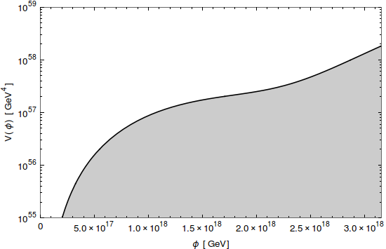
Figure 1: RGE-improved inflaton quartic potential plotted against $\phi$. $M=M_{P}=2.43\times 10^{18}$ GeV.

We note a crucial point at the end of this section to carry forward to the next section: that the inflection-point and the inflationary plateau-like behaviour necessarily leads to $\lambda_{\phi}\simeq 0$ and $\beta_{\lambda_{\phi}}\simeq 0$ at M (UV scale) which means that in our model due to the presence of the Yukawa coupling $y$, $\lambda_{\phi}$ monotonically grows in the IR from UV. In the next section, we will see that for the requirement of radiative symmetry breaking via CW mechanism, we will also need positive contribution in $\beta_{\lambda_{\phi}}$ to dominate in order to have negative $\lambda_{\phi}$ in the IR.

III Coleman-Weinberg in the IR

In this section we present the Coleman-Weinberg pathway to generate the EW and Seesaw scales in the IR. Such a scenario demands as we will show to be difficult to achieve the inflationary-plateau behaviour as described in the last section. We will present a possible resolution to the problem by implementing energy threshold correction and derive the full sets of conditions on the parameters of the model that lead to the whole picture to be consistent.

III.1 Dynamical Generation of EW and $B-L$ Seesaw Scales

As discussed in section. II.2, we work with gauge group $\rm U(1)_{Y}\times SU(2)_{L}\times SU(3)_{c}\times U(1)_{B-L}$, namely the SM gauge group with an extra $U(1)_{B-L}$. At low energy, we have dynamical symmetry breaking down to ${\rm U}(1)_{\rm em}\times SU(3)_{c}$ gauge group. However, as we do not have any dimensionful parameter in the Lagrangian, we depend on dynamical generation of scales through running of couplings. To discuss the basics of this dynamical generation, we consider $\beta_{\lambda_{\phi}}$ in Eq. 14. If there is no fermionic contribution, we get,

$$\phi\frac{d\lambda_{\phi}}{d\phi}=\frac{1}{16\pi^{2}}\left(20\lambda_{\phi}^{2}+96g_{BL}^{4}-48\lambda_{\phi}g_{BL}^{2}\right).$$ (22)

As a consequence, when there is no negative Yukawa contribution, $\beta_{\lambda_{\phi}}$ is positive definite and the $g_{BL}$ term makes $\lambda_{\phi}$ negative at low energy, leading to dynamically generated vev of $\phi$, $v_{BL}$.

The effective scalar potential at one loop order can be approximated by inserting a running $\lambda_{\phi}$ in the tree-level potential of Eq.15:

$$V(\phi)\simeq\frac{1}{4}\lambda_{\phi}\phi^{4}\simeq\frac{1}{4}\beta_{\lambda_{\phi}}\ln(\phi/\phi_{*})\phi^{4},$$ (23)

where $\phi_{*}$ is the critical scale below which $\lambda_{\phi}$ becomes negative. The potential attains a minima as $\lambda_{\phi}$ is negative at small energy scales, as discussed latter in section, IV. Once $\phi$ attains a vev, the mixing $-\lambda_{H\phi}|H|^{2}|\phi|^{2}$ works as the symmetry breaking term of SM Higgs, the mass matrix analysis of the system will be discussed latter in section. IV.

Effectively we can say that $\phi$ acts as ‘the Higgs of the $B-L$ Higgs’ and as ‘the Higgs of Seesaw Scale’. Furthermore, the ‘Higgs of the $\phi$’ is $\phi$ itself, i.e. the EW scale and the seesaw scale are dynamically generated via dimensional transmutation when $U(1)_{B-L}$ symmetry is broken radiatively, i.e. $\lambda_{\phi}<0$.

III.2 Difficulty with Inflection-point Conditions

However, as discussed in section. II, at the scale of plateau inflation $\phi=M$, $\beta_{\lambda_{\phi}}\simeq 0$ due to cancellation of the bosonic and fermionic contributions, i.e. $\beta_{\lambda_{\phi}}\simeq 96g_{BL}^{4}-2y^{4}=0$, considering the dominant contributions in Eq. 14. As the inflaton field $\phi$ rolls down the potential to scales below the scale of the inflationary plateau around M, the fermionic contributions $\sim y^{4}$ becomes dominant and $\beta_{\lambda_{\phi}}<0$. So, it seems impossible to make $\lambda_{\phi}$ negative in the IR again just using radiative corrections.

III.3 Achieving the Inflationary Plateau via Threshold Correction

One possible resolution to achieve the inflection-point at UV and $\lambda_{\phi}<0$ at IR simultaneously in a model maybe possible through threshold energy corrections, i.e. going from UV to IR, if at some scale, say $\mu_{T}$, a fermionic contribution $2y^{4}$ to $\beta_{\lambda_{\phi}}$ vanishes, the bosonic contribution $96g_{BL}^{4}$ again dominates, making $\beta_{\lambda_{\phi}}>0$ again in the IR. This makes it possible for $\lambda_{\phi}<0$ and forces the $U(1)_{B-L}$ symmetry breaking, á lá CW mechanism.

We lay out the prescription for this mechanism in the model II.2: in our model the additional $B-L$ Higgs $\phi$ as the inflaton interacts with right-handed neutrinos ($N_{R}^{i}$) and vector-like fermions ($\psi_{L,R}$) through Yukawa interaction terms, $Y_{j}^{low},~{}y_{L}$ and $y_{R}$ respectively, as per Eq. 12 in the UV but stop affecting the RGE-improved potential in the IR due to threshold correction, at a scale $\mu_{T}$; RGE below the threshold energy scale $\mu=\mu_{T}$ becomes (eliminating the contribution of $y_{L}$ and $y_{R}$ in Eq. 14),

$$\phi\frac{d\lambda_{\phi}}{d\phi} = \frac{1}{16\pi^{2}}\left(20\lambda_{\phi}^{2}+96g_{BL}^{4}-\sum_{j}Y_{j}^{low~{}4}+\lambda_{\phi}\left(2\sum_{j}Y_{j}^{low~{}2}-48g_{BL}^{2}\right)\right),$$ (24)

Besides the scale of inflection-point M, we have the threshold scale $\mu_{T}$ as the only free parameter in our model. We shall see later that $\mu_{T}$ has a lower bound depending on $g_{BL}$, hence $M$, if we assume that RGEs of Dark sector and SM sector evolve independently. If $Y_{i}^{low}\ll y_{L,R}$ and $Y_{i}^{low}\ll g_{BL}$, the value of $\lambda_{\phi}$ suddenly drops to negative value below $\mu_{T}$ ( as shown in Fig. 2). The sudden drop is due to the fact that $-48\lambda_{\phi}g_{BL}^{2}$ is negligibly small with respect to $96g_{BL}^{4}$ (see Eq.24). If the difference between the contributions $-48\lambda_{\phi}g_{BL}^{2}$ and $96g_{BL}^{4}$ is smaller, we may achieve a smooth transition of $\lambda_{\phi}$ from positive to negative values. For the choice of parameters $\mu_{T}=44.85$ TeV , $M=M_{P}$ and choosing negligible $Y^{low}=10^{-3}y$, the evolution of the couplings are shown in Fig. 2.

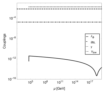
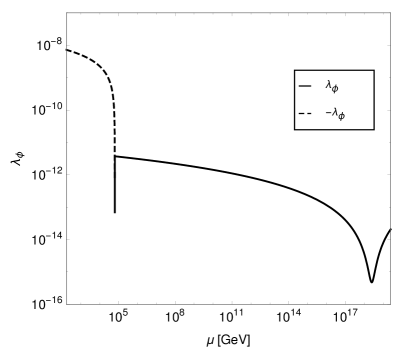
Figure 2: Left Panel: RG running of all the couplings for the benchmark point (M = 1 $M_{P}$, $\mu_{T}=44.85$ TeV) against $\mu$. Right Panel: RG running of $\lambda_{\phi}$ against $\mu$. Note the abrupt drop of $\lambda_{\phi}$ to negative value at the threshold. We have chosen negligible $Y^{low}=10^{-3}y$ for this work.

In summary, to start with we had six parameters in our model, namely the scale of inflationary plateau $M$, the threshold scale $\mu_{T}$, and the couplings $\lambda_{\phi},~{}g_{BL},~{}y,~{}Y^{low}$. Among them we choose $Y^{low}\ll y$ and $Y^{low}\ll g_{BL}$, such that they do not affect the RGE-improved inflationary potential V($\phi$) thus leaving us with 5 parameters. Fixing the observed values of the inflationary parameters $P^{2}_{\mathcal{R}}$, $n_{s}$ and a chosen value of e-foldings $N$ makes the couplings $\lambda_{\phi},~{}g_{BL},~{}y$ at $\phi=M$ dependent only on $M$, therefore reducing the system to only two independent parameters $M$ and $\mu_{T}$ in totality in our model.

III.4 Conditions for Theoretical Consistencies

In order to simplify our model we assume that RGEs of the dark sector and SM sector evolve independently of each other, as previously mentioned in section. II.2. To satisfy this assumption we require that the positive contribution of $\lambda_{H\phi}^{2}$ in $\beta_{\lambda_{\phi}}$ to be negligible w.r.t the contribution from gauge coupling $g_{BL}^{4}$ in Eq. 14, i.e. $8\lambda_{H\phi}^{2}<96g_{BL}^{4}$. In the other extreme of this assumption, i.e. for $8\lambda_{H\phi}^{2}>96g_{BL}^{4}$, the inflection point is achieved via cancellation of contributions from $\lambda_{H\phi}^{2}$ and $y^{4}$ in $\beta_{\lambda_{\phi}}$, however we do not discuss this scenario in this work (see Caputo (2019b) for such an example). Now, the term $-\lambda_{H\phi}\,|H|^{2}\phi^{2}$ in the scalar potential, when $\phi=\langle\phi\rangle=v_{BL}/\sqrt{2}$, works as $-m^{2}|H|^{2}$ (where $m=m_{h}/\sqrt{2}=88$ GeV, $m_{h}=125$ GeV being the mass of SM Higgs) to provide spontaneous symmetry breaking of SM Higgs, so we get $m_{h}^{2}=\lambda_{H\phi}v_{BL}^{2}$. As for our case $\mu_{T}\sim v_{BL}/\sqrt{2}$ (due to the sharp drop of $\lambda_{\phi}$ at $\mu_{T}$), we get a lower limit of $\mu_{T}$, i.e.

$$\mu_{T}\gtrsim\frac{v_{BL}}{\sqrt{2}}=\frac{m}{\sqrt{\lambda_{H\phi}}}>\frac{m}{(2\sqrt{3}g_{BL}^{2})^{1/2}}.$$ (25)

This condition also gives us a lower limit on $m_{Z_{BL}}$,

$$m_{Z_{BL}}=2g_{BL}v_{BL}>\frac{2\sqrt{2}g_{BL}m}{(2\sqrt{3}g_{BL}^{2})^{1/2}}=\frac{2}{3^{1/4}}m=133~{}\rm GeV$$ (26)

In terms of order-of-magnitude estimate, this will be truly valid for $8\lambda_{H\phi}^{2}\ll 96g_{BL}^{4}$, setting $8\lambda_{H\phi}^{2}$ to be $\lesssim 10g_{BL}^{4}$, requiring $m_{Z_{BL}}>3\times 133~{}\rm GeV$. This we chose to be our lower bound on $m_{Z_{BL}}$. This condition translated to $M$ as the lower bound for some chosen value of $\mu_{T}$, along with the upper bound condition from Eq.21 will assure us the theoretical consistency of our analysis and results.

Along with this bound of $m_{Z_{BL}}>3\times 133~{}\rm GeV$, we have a stronger bound on $m_{Z_{BL}}$ from the theoretical consistency of our analysis, as will be discussed in the section IV. This bound comes from the calculation of masses of the scalar mass eigenstates. The constraint we use in this work is,

$$m_{Z_{BL}}\gtrsim 850~{}\rm GeV.$$ (27)

IV Reheating the Visible Universe

Now let us turn towards the reheating dynamics to connect our model with the standard Big Bang Cosmology. This occurs when inflation has terminated and the inflaton oscillates around the minima of its potential, interpreted as a collection of particles at rest and decays perturbatively. The reheating temperature $T_{rh}$ is then given by,

$$T_{rh}\simeq.55\left(\frac{100}{g_{*}}\right)^{1/4}\sqrt{\Gamma_{\varphi}M_{P}};$$ (28)

where $\Gamma_{\varphi}$ is the decay rate of the redefined inflaton $\varphi=\sqrt{2}\texttt{Re}(\phi)$ and $g_{*}$ is the number of SM degrees of freedom. To calculate $\Gamma_{\varphi}$, we first calculate the mass of the inflaton $m_{\varphi}$ from the numerically calculated second derivative of the RGE improved potential at the minima $v_{BL}/\sqrt{2}$, $V^{\prime\prime}(\phi)|_{\phi=v_{BL}/\sqrt{2}}=m_{\phi}^{2}=2m_{\varphi}^{2}$. For our benchmark point of $M=M_{P}$ and $\mu_{T}=44.85$ TeV, we have $v_{BL}=49.1$ TeV as shown in Fig. 3, and $m_{\varphi}=0.85$ GeV.

We now note that the SM Higgs boson mass ($m_{h}=125$ GeV) is given by,

$$m_{h}^{2}=\lambda_{H\phi}v_{BL}^{2},$$ (29)

where $v_{H}=246$ GeV is the Higgs doublet VEV.

The mass matrix of the Higgs bosons, $\varphi$ and $h$, is given by,

$${\cal L}\supset-\frac{1}{2}\begin{bmatrix}h&\varphi\end{bmatrix}\begin{bmatrix}m_{h}^{2}&\lambda_{H\phi}v_{BL}v_{H}\\ \lambda_{H\phi}v_{BL}v_{H}&m_{\varphi}^{2}\end{bmatrix}\begin{bmatrix}h\\ \varphi\end{bmatrix}.$$ (30)

Diagonalising the mass matrix by

$$\begin{bmatrix}h\\ \varphi\end{bmatrix}=\begin{bmatrix}\cos\theta&\sin\theta\\ -\sin\theta&\cos\theta\end{bmatrix}\begin{bmatrix}{\tilde{h}}\\ {\tilde{\varphi}}\end{bmatrix},$$ (31)

where ${\tilde{h}}$ and ${\tilde{\varphi}}$ are the mass eigenstates, and the mixing angle $\theta$ determined by

$$2v_{BL}v_{H}\lambda_{H\phi}=(m_{h}^{2}-m_{\varphi}^{2})\tan 2\theta,$$ (32)

we find, for $m_{\varphi}^{2}\ll m_{h}^{2}$ and $\lambda_{H\phi}\ll 1$,

$$\theta\simeq\frac{v_{H}}{v_{BL}}.$$ (33)

The mass eigenvalues are then given by

$$m_{\tilde{\varphi}}^{2}=m_{\varphi}^{2}+\left(m_{\varphi}^{2}-m_{h}^{2}\right)\frac{\sin^{2}\theta}{1-2\sin^{2}\theta}\simeq m_{\varphi}^{2}-m_{h}^{2}\theta^{2},$$

$$m_{\tilde{h}}^{2}=m_{h}^{2}-\left(m_{\varphi}^{2}-m_{h}^{2}\right)\frac{\sin^{2}\theta}{1-2\sin^{2}\theta}\simeq m_{h}^{2}.$$ (34)

For the parameter values we are interested in, we find $m_{\tilde{\varphi},{\tilde{h}}}\simeq m_{\varphi,h}$ and $\tilde{\phi},\tilde{h}\simeq\phi,h$. We noted that, for this mass eigenstate approximations to make sense numerically, i.e. to really get $m_{\tilde{\varphi},{\tilde{h}}}\simeq m_{\varphi,h}$, we require approximately $m_{Z_{BL}}\gtrsim 850~{}\rm GeV$. So, for notational simplicity, we will refer to the mass eigenstates without using tilde in the rest of this work.

Coming back to our benchmark point of $M=M_{P}$ and $\mu_{T}=44.85$ TeV, the inflaton decays into SM particles through mixing with SM Higgs, with the mixing angle $\theta\simeq\frac{v_{H}}{v_{BL}}=\frac{246}{\sqrt{2}~{}49.1\times 10^{3}}$. The dominant decay channel of the inflaton with mass $m_{\varphi}=0.85$ GeV is into strange quark or muon pairs. This decay rate of the inflaton is then given by,

$$\Gamma_{\varphi}=\Gamma_{H}\sin^{2}\theta\simeq\left(\frac{3}{8\pi}\frac{m_{s}^{2}}{v_{H}^{2}}m_{\varphi}+\frac{1}{8\pi}\frac{m_{\mu}^{2}}{v_{H}^{2}}m_{\varphi}\right)\sin^{2}\theta,$$ (35)

where $\Gamma_{H}$ is the SM Higgs decay rate into pairs of SM particles with mass $<m_{\varphi}/2$ and $m_{s}\sim 96$ MeV, $m_{\mu}\sim 105$ MeV denotes mass of strange quark and muon particles respectively. This decay leads to the reheating temperature of $T_{rh}\simeq 635~{}\rm GeV.$

For the benchmark points $M=5.67$ and $0.1~{}M_{P}$, respectively $\mu_{T}=48.53$ and $96.63$ TeV, we get $v_{BL}=52.73$ and $106.06$ TeV, $m_{\phi}=2.93$ GeV (dominant decay channel into charm quark pair) and $0.39$ GeV (dominant decay channel into strange quark and muon pairs). Following the same prescription given in this section earlier, we get $T_{rh}\simeq 12.3$ TeV and $198.02$ GeV respectively. So, all three benchmark points have $T_{rh}>1$ MeV (scale of BBN).

It is important to mention that to calculate a more realistic reheating temperature we need to solve the field dynamics after inflation in $\phi-H$ plane. This is because whenever the field trajectory has a component in the SM Higgs direction, which is indeed the case near the minima of the potential, we get a sudden suppression in the energy density in the fields due to high decay rate of the SM Higgs, hence helping the reheating cause. However calculating this dynamics is complex in our case due to sudden sharp edges of the potential near the threshold scale $\mu_{T}$, and we omit this analysis in this work. Keeping this in mind, we state that the $T_{rh}$ estimates we have done are more conservative, hence having this conservative estimates well over the BBN scale is enough for our bench mark points to be consistent with the standard Big Bang Cosmology.

We also mention that the reheating temperature $T_{rh}$ is far smaller than the inflationary Hubble scale, $\mathcal{H}_{inf}=\frac{1}{\sqrt{3}M_{P}}\sqrt{V(\phi)|_{\phi=M}}$. For the benchmark points (M = 5.67 $M_{P}$, $\mu_{T}=$48.53 TeV), (M = 1 $M_{P}$, $\mu_{T}=44.85$ TeV) and ($M=0.1~{}M_{P}$, $\mu_{T}=96.63$ TeV), scales of inflation are $\mathcal{H}_{inf}=2.79\times 10^{12}$ GeV, $1.53\times 10^{10}$ GeV and $1.53\times 10^{7}$ GeV respectively, in contrast to $T_{rh}$ in the TeV scale.

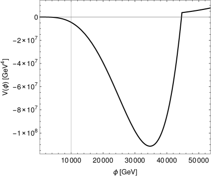
Figure 3: Plot of $V(\phi)$ for the benchmark point (M = 1 $M_{P}$, $\mu_{T}=44.85$ TeV) near the threshold scale and minima of the potential in IR. Note that due to the sharp drop in potential to the minima near $\phi=\mu_{T}$, we can use the approximation $v_{BL}/\sqrt{2}\sim\mu_{T}$.

V Model Constraints from LHC

In this section we will discuss the constraints on our model parameters that come from the gauge boson search in hadron colliders, via the s-channel process $p+p\to Z^{\prime}\to e^{+}e^{-}/\mu^{+}\mu^{-}$.

For computing cross-section for LHC processes, $g_{BL}$ is already constrained to be small, and we interpret the $Z^{\prime}$ search to be equivalent to $Z_{BL}$ search. The cross-section for the process $\sigma(pp\to Z_{BL}\to e^{+}e^{-}/\mu^{+}\mu^{-})\simeq\sigma(pp\to Z_{BL}){\rm BR}(Z_{BL}\to e^{+}e^{-}/\mu^{+}\mu^{-})$ in the narrow-width approximation,

$$\sigma(pp\to Z_{BL})=2\sum_{q,\overline{q}}\int dx\int dy\,f_{q}(x,Q)f_{\overline{q}}(y,Q)\hat{\sigma}(\hat{s}),$$ (36)

with

$$\hat{\sigma}(\hat{s})=\frac{4\pi^{2}}{3}\frac{\Gamma(Z_{BL}\to q\overline{q})}{M_{Z_{BL}}}\delta(\hat{s}-M_{Z^{\prime}}^{2}).$$ (37)

where $f_{q}$ and $f_{\overline{q}}$ represent the parton distribution functions for a quark and an anti-quark, $\hat{s}\equiv xys$ represent the invariant squared mass of the quarks in collision. In our LHC Run-2 analysis we will follow Ref. Aad et al. (2019) which is for the c.o.m $\sqrt{s}=13\;{\rm TeV}$.

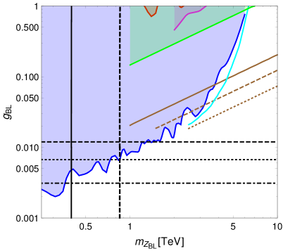
Figure 4: Left Panel: The horizontal lines correspond to the inflection-point scale M = 5.67 $M_{P}$ (dashed), $M_{P}$ (dotted) and 0.1 $M_{P}$ (dot-dashed) respectively . This corresponds to $m_{Z_{BL}}$ lower bounds to be 1.64 TeV, 850 GeV and 360 GeV respectively, when taken into account $B-L$ gauge coupling limit from ATLAS di-lepton result, as mentioned later. The vertical solid line and the vertical thick dashed line correspond to $m_{Z_{BL}}=3\times 133$ and $850$ GeV respectively, the lower limit for theoretical consistency as discussed in the text. The jagged blue solid line is the upper bound on the $B-L$ gauge coupling as a function of $Z_{BL}$ mass from the ATLAS dileption final result (ATLAS-CONF-2019-001) ATL (2019a). We also explicitly show the other current constraints (dashed region): Green corresponds to LEP-II Schael et al. (2013), Magenta and Red are bounds obtained from ATLAS13 (2j)ATL (2019b), CMS13 (2j)Sirunyan et al. (2018). Cyan ATLAS-TDR (2l)CER (2017). Brown solid, dashed, dotted are for future e+e- colliders with $\sqrt{s}=$ 250, 500 and 1000 GeV. The LEP and the future e+e- collider bounds were obtained using contact interaction strategy in the Refs.Das et al. (2021, 2022). Right Panel: Plot of $M/M_{P}$ versus $\mu_{T}$ (TeV). Using the relation $m_{Z_{BL}}=2g_{BL}v_{BL}\sim 2\sqrt{2}g_{BL}\mu_{T}$, it has been mapped to $M/M_{P}$ vs $\mu_{T}$ parameter space via Eq.19. The open parameter region bound from right by $M=5.67~{}M_{P}$, from bottom by the ATLAS final result and from left by the thick dashed curve corresponding to $m_{Z_{BL}}=850$ GeV is allowed within our theoretical framework and experimental constraints.

Current experimental constraints in the $m_{Z_{BL}}$ vs $g_{BL}$ parameter space corresponding to $B-L$ vector boson (as shown in left panel of Fig. 4), with mass $m_{Z_{BL}}=2g_{BL}v_{BL}$, can be mapped to $M/M_{P}$ vs $\mu_{T}$ parameter space of our model using Eq.19 and the expression $m_{Z_{BL}}=2g_{BL}v_{BL}\sim 2\sqrt{2}g_{BL}\mu_{T}$. Constraints from these experiments mentioned before into $M/M_{P}$ vs $\mu_{T}$ parameter space is shown in the right panel of Fig. 4.

As one can see from Fig. 2, g_BL and $y$ and $Y_{low}$ remains almost constant throughout the RGE evolution. When the $U(1)_{B-L}$ symmetry is broken, the $Z^{\prime}$ boson becomes massive with its $M_{Z^{\prime}}=2g_{BL}v_{BL}$. Fig. 4 benchmark points (M = 0.1 Mp, M = Mp, 5.67 Mp) on the $m_{Z_{BL}}$-$g_{BL}(M_{\rm P})$ plane, computed at the $U(1)_{B-L}$ breaking scale $\mu=\phi=v_{BL}/\sqrt{2}$. The plots clearly indicate for $g_{BL}\sim O(10^{-2})$ the mass $Z_{BL}$ boson can be of $\mathcal{O}(TeV)$ to satisfy all constraints. For lower $g_{BL}$ values even lighter $Z_{BL}$ mass is allowed, upto $\sim 850$ GeV.

In terms of the free parameters of the model, namely $\mu_{T}$ and M, it can be seen from right panel of Fig. 4 that $\mu_{T}\lesssim 50$ TeV is excluded by LHC run-2 data. Note that the analysis is only consistent within the open region limited by $M<5.67~{}M_{P}$ and the curve corresponding to the condition $m_{Z_{BL}}>850$ GeV.

VI Discussion & Conclusion

We investigated in a minimal $B-L$ conformal extension of the SM the possibility of the $B-L$ Higgs driving inflation in the UV (without any coupling to gravity). In this model, starting from the UV, we explicitly derived the conditions in order to mimic the SM Higgs mass generating mechanism dynamically via perturbative quantum corrections, á lá Coleman-Weinberg in the IR. The main findings of the paper are as follows:

• Cosmic inflation happens due to the flatness of the U$(1)_{B-L}$ Higgs potential achieved through bosonic and fermionic quantum corrections. Once the inflection-point scale M is fixed, the values of the free parameters of the model, namely, $\lambda_{\phi},~{}g_{BL},~{}y$ are fixed at the scale M, and its running via RGE determines its value at the lower EW scale.

• Due the nature of the running of $\lambda_{\phi}$ near the threshold correction energy scale $\mu_{T}$, the seesaw scale $v_{BL}/\sqrt{2}\sim\mu_{T}$ is a good approximation (see Figs. 2 and 3).

• Besides M, the only free parameter in the model is the threshold energy scale $\mu_{T}$ ($\sim v_{BL}/\sqrt{2}$), i.e. the scale at which $U(1)_{B-L}$ symmetry is broken. Once the symmetry is broken happens, $\phi$ obtains VEV $v_{BL}$ and a term similar to $-m^{2}|H|^{2}$ comes into play, mimicking the SM Higgs mechanism á lá Coleman-Weinberg. The condition for the SM Higgs mass generation determines the combination $\lambda_{H\phi}\mu_{T}^{2}$ as $m_{h}^{2}=\lambda_{H\phi}v_{BL}^{2}\sim 2\lambda_{H\phi}\mu_{T}^{2}$. Therefore, $\lambda_{H\phi}$ is fixed from Higgs VEV (246 GeV), once $\mu_{T}$ is fixed.

• Considering $Z_{BL}$ searches in LHC, particularly upper limits from ATLAS, we get $\mu_{T}\sim v_{BL}/\sqrt{2}\leq O(80)$ TeV is excluded (see Fig. 4).

• The model predicts $m_{Z_{BL}}\geq$ 2 TeV with $g_{BL}\sim O(10^{-2})$ to be consistent with the inflationary cosmology, dynamical generation of EW and Seesaw scales as well as allowed by LHC searches. Such a region will be within the reach of future experiments.

• For the benchmark points (M = 5.67 $M_{P}$, $\mu_{T}=$48.53 TeV), (M = 1 $M_{P}$, $\mu_{T}=44.85$ TeV) and ($M=0.1~{}M_{P}$, $\mu_{T}=96.63$ TeV) considered in the model we estimated the reheating temperature $T_{rh}\simeq$ 12.3 TeV, 635 GeV and 198.0 GeV respectively and the scales of inflation to be $\mathcal{H}_{inf}=2.79\times 10^{12}$ GeV, $1.53\times 10^{10}$ GeV and $1.53\times 10^{7}$ GeV respectively, thus being consistent with BBN limits.

Conformal invariance dictates no scales are fundamental in nature. We showed here that the dynamical scale generation of electroweak physics (EW), heavy neutrino physics (seesaw scale) and the phenomena of inflation can be achieved together purely via quantum corrections in particle theory of fundamental interactions and put constraints and predicted signatures in collider physics. To derive the Coleman-Weinberg potential, we only considered 1-loop fluctuations due to the bosonic and fermionic degrees of freedom. Since our model is minimally coupled to gravity, we do not expect the picture to change due to quantum corrections from the gravity sector. Finally, this work can be extended by a full two-field study of inflation and its effect on primordial non-Gaussianities (see, e.g. Ref. Wands (2008) for a review) or other observables like Primordial Blackholes (PBH) (see e.g. Ref. Garcia-Bellido and Ruiz Morales (2017)) and secondary Gravitational Waves predictions (see e.g. Ref. Domènech (2021)).

We envisage that our studies concerning the conformal invariance at the classical level, the interplay of dynamical mass scale generation in the IR and cosmic inflation in UV will open up a new direction in future to unified model-buildings in BSM theories, having to explain the dark matter, matter-antimatter asymmetry, inflation, Strong CP and the EW-Planck scales hierarchy problems, under one umbrella, with or without gravity, and have testable laboratory, astrophysical or cosmic observable predictions.

VII Acknowledgements

A.G. and A.P. thanks Arindam Das for discussions. This work is supported in part by the United States, Department of Energy Grant No. DE-SC0012447 (N.O.).

References

- Guth (1981) A. H. Guth, Phys. Rev. D 23, 347 (1981).
- Sato (1981) K. Sato, Mon. Not. Roy. Astron. Soc. 195, 467 (1981).
- Kazanas (1980) D. Kazanas, Astophys.J. 241, L59 (1980).
- Nariai and Tomita (1971) H. Nariai and K. Tomita, Progress of Theoretical Physics 46, 776 (1971).
- Starobinsky (1980) A. Starobinsky, Physics Letters B 91, 99 (1980).
- Akrami et al. (2020) Y. Akrami et al. (Planck), Astron. Astrophys. 641, A10 (2020), arXiv:1807.06211 [astro-ph.CO] .
- Bezrukov and Shaposhnikov (2008) F. L. Bezrukov and M. Shaposhnikov, Phys. Lett. B 659, 703 (2008), arXiv:0710.3755 [hep-th] .
- Libanov et al. (1998) M. Libanov, V. Rubakov, and P. Tinyakov, Phys. Lett. B 442, 63 (1998), arXiv:hep-ph/9807553 .
- Fakir and Unruh (1990) R. Fakir and W. Unruh, Phys. Rev. D 41, 1783 (1990).
- Futamase and Maeda (1989) T. Futamase and K.-i. Maeda, Phys. Rev. D 39, 399 (1989).
- Masina (2018) I. Masina, Phys. Rev. D 98, 043536 (2018), arXiv:1805.02160 [hep-ph] .
- Okada et al. (2010) N. Okada, M. U. Rehman, and Q. Shafi, Phys. Rev. D 82, 043502 (2010), arXiv:1005.5161 [hep-ph] .
- Linde (1987) A. D. Linde, Adv. Ser. Astrophys. Cosmol. 3, 149 (1987).
- Kallosh et al. (1995) R. Kallosh, A. D. Linde, D. A. Linde, and L. Susskind, Phys. Rev. D 52, 912 (1995), arXiv:hep-th/9502069 .
- Inagaki et al. (2014) T. Inagaki, R. Nakanishi, and S. D. Odintsov, Astrophys. Space Sci. 354, 2108 (2014), arXiv:1408.1270 [gr-qc] .
- Okada et al. (2017) N. Okada, S. Okada, and D. Raut, Phys. Rev. D 95, 055030 (2017), arXiv:1702.02938 [hep-ph] .
- Choi and Lee (2016a) S.-M. Choi and H. M. Lee, Eur. Phys. J. C 76, 303 (2016a), arXiv:1601.05979 [hep-ph] .
- Allahverdi et al. (2006) R. Allahverdi, K. Enqvist, J. Garcia-Bellido, and A. Mazumdar, Phys. Rev. Lett. 97, 191304 (2006), arXiv:hep-ph/0605035 .
- Allahverdi et al. (2007) R. Allahverdi, K. Enqvist, J. Garcia-Bellido, A. Jokinen, and A. Mazumdar, JCAP 06, 019 (2007), arXiv:hep-ph/0610134 .
- Bueno Sanchez et al. (2007) J. C. Bueno Sanchez, K. Dimopoulos, and D. H. Lyth, JCAP 01, 015 (2007), arXiv:hep-ph/0608299 .
- Baumann et al. (2007) D. Baumann, A. Dymarsky, I. R. Klebanov, L. McAllister, and P. J. Steinhardt, Phys. Rev. Lett. 99, 141601 (2007), arXiv:0705.3837 [hep-th] .
- Baumann et al. (2008) D. Baumann, A. Dymarsky, I. R. Klebanov, and L. McAllister, JCAP 01, 024 (2008), arXiv:0706.0360 [hep-th] .
- Badziak and Olechowski (2009) M. Badziak and M. Olechowski, JCAP 02, 010 (2009), arXiv:0810.4251 [hep-th] .
- Enqvist et al. (2010) K. Enqvist, A. Mazumdar, and P. Stephens, JCAP 06, 020 (2010), arXiv:1004.3724 [hep-ph] .
- Cerezo and Rosa (2013) R. Cerezo and J. G. Rosa, JHEP 01, 024 (2013), arXiv:1210.7975 [hep-ph] .
- Choudhury et al. (2013) S. Choudhury, A. Mazumdar, and S. Pal, JCAP 07, 041 (2013), arXiv:1305.6398 [hep-ph] .
- Choudhury and Mazumdar (2014) S. Choudhury and A. Mazumdar, (2014), arXiv:1403.5549 [hep-th] .
- Ballesteros and Tamarit (2016a) G. Ballesteros and C. Tamarit, JHEP 02, 153 (2016a), arXiv:1510.05669 [hep-ph] .
- Okada and Raut (2017) N. Okada and D. Raut, Phys. Rev. D 95, 035035 (2017), arXiv:1610.09362 [hep-ph] .
- Stewart (1997a) E. D. Stewart, Phys. Lett. B 391, 34 (1997a), arXiv:hep-ph/9606241 .
- Stewart (1997b) E. D. Stewart, Phys. Rev. D 56, 2019 (1997b), arXiv:hep-ph/9703232 .
- Drees and Xu (2021) M. Drees and Y. Xu, JCAP 09, 012 (2021), arXiv:2104.03977 [hep-ph] .
- Okada et al. (2019) N. Okada, D. Raut, and Q. Shafi, (2019), arXiv:1910.14586 [hep-ph] .
- Okada and Raut (2019) N. Okada and D. Raut, (2019), arXiv:1910.09663 [hep-ph] .
- Ballesteros and Tamarit (2016b) G. Ballesteros and C. Tamarit, JHEP 02, 153 (2016b), arXiv:1510.05669 [hep-ph] .
- Choi and Lee (2016b) S.-M. Choi and H. M. Lee, Eur. Phys. J. C 76, 303 (2016b), arXiv:1601.05979 [hep-ph] .
- Bai and Stolarski (2020) Y. Bai and D. Stolarski, (2020), arXiv:2008.09639 [hep-ph] .
- Dimopoulos et al. (2018) K. Dimopoulos, C. Owen, and A. Racioppi, Astropart. Phys. 103, 16 (2018), arXiv:1706.09735 [hep-ph] .
- Caputo (2019a) A. Caputo, Phys. Lett. B 797, 134824 (2019a), arXiv:1902.02666 [hep-ph] .
- Senoguz and Shafi (2008) V. N. Senoguz and Q. Shafi, Phys. Lett. B 668, 6 (2008), arXiv:0806.2798 [hep-ph] .
- Enqvist and Karciauskas (2014) K. Enqvist and M. Karciauskas, JCAP 02, 034 (2014), arXiv:1312.5944 [astro-ph.CO] .
- Okada et al. (2021) N. Okada, D. Raut, and Q. Shafi, Phys. Lett. B 812, 136001 (2021), arXiv:1910.14586 [hep-ph] .
- Ghoshal et al. (2018a) A. Ghoshal, A. Mazumdar, N. Okada, and D. Villalba, Phys. Rev. D 97, 076011 (2018a), arXiv:1709.09222 [hep-th] .
- Ghoshal (2019a) A. Ghoshal, Int. J. Mod. Phys. A 34, 1950130 (2019a), arXiv:1812.02314 [hep-ph] .
- Ghoshal et al. (2021a) A. Ghoshal, A. Mazumdar, N. Okada, and D. Villalba, Phys. Rev. D 104, 015003 (2021a), arXiv:2010.15919 [hep-ph] .
- Frasca and Ghoshal (2021a) M. Frasca and A. Ghoshal, Class. Quant. Grav. 38, 175013 (2021a), arXiv:2011.10586 [hep-th] .
- Frasca and Ghoshal (2020a) M. Frasca and A. Ghoshal, JHEP 21, 226 (2020a), arXiv:2102.10665 [hep-th] .
- Frasca et al. (2022a) M. Frasca, A. Ghoshal, and A. S. Koshelev, (2022a), arXiv:2202.09578 [hep-ph] .
- Biswas and Okada (2015) T. Biswas and N. Okada, Nucl. Phys. B 898, 113 (2015), arXiv:1407.3331 [hep-ph] .
- Su et al. (2021) X.-F. Su, Y.-Y. Li, R. Nicolaidou, M. Chen, H.-Y. Wu, and S. Paganis, Eur. Phys. J. C 81, 796 (2021), arXiv:2108.10524 [hep-ph] .
- Gross and Wess (1970) D. J. Gross and J. Wess, Phys. Rev. D 2, 753 (1970).
- Callan et al. (1970) C. G. Callan, S. Coleman, and R. Jackiw, Annals of Physics 59, 42 (1970).
- Coleman and Jackiw (1971) S. R. Coleman and R. Jackiw, Annals Phys. 67, 552 (1971).
- Coleman and Weinberg (1973a) S. Coleman and E. Weinberg, Phys. Rev. D 7, 1888 (1973a).
- Englert et al. (2013) C. Englert, J. Jaeckel, V. Khoze, and M. Spannowsky, JHEP 04, 060 (2013), arXiv:1301.4224 [hep-ph] .
- Adler (1982) S. L. Adler, Rev. Mod. Phys. 54, 729 (1982), [Erratum: Rev.Mod.Phys. 55, 837 (1983)].
- Coleman and Weinberg (1973b) S. R. Coleman and E. J. Weinberg, Phys. Rev. D 7, 1888 (1973b).
- Salvio and Strumia (2014) A. Salvio and A. Strumia, JHEP 06, 080 (2014), arXiv:1403.4226 [hep-ph] .
- Einhorn and Jones (2015) M. B. Einhorn and D. R. T. Jones, JHEP 03, 047 (2015), arXiv:1410.8513 [hep-th] .
- Einhorn and Jones (2016a) M. B. Einhorn and D. T. Jones, JHEP 05, 185 (2016a), arXiv:1602.06290 [hep-th] .
- Einhorn and Jones (2016b) M. B. Einhorn and D. R. T. Jones, JHEP 01, 019 (2016b), arXiv:1511.01481 [hep-th] .
- Khoze (2013) V. V. Khoze, JHEP 11, 215 (2013), arXiv:1308.6338 [hep-ph] .
- Kannike et al. (2014) K. Kannike, A. Racioppi, and M. Raidal, JHEP 06, 154 (2014), arXiv:1405.3987 [hep-ph] .
- Rinaldi et al. (2015) M. Rinaldi, G. Cognola, L. Vanzo, and S. Zerbini, Phys. Rev. D 91, 123527 (2015), arXiv:1410.0631 [gr-qc] .
- Kannike et al. (2015a) K. Kannike, G. Hütsi, L. Pizza, A. Racioppi, M. Raidal, A. Salvio, and A. Strumia, JHEP 05, 065 (2015a), arXiv:1502.01334 [astro-ph.CO] .
- Kannike et al. (2015b) K. Kannike, G. Hütsi, L. Pizza, A. Racioppi, M. Raidal, A. Salvio, and A. Strumia, PoS EPS-HEP2015, 379 (2015b).
- Barrie et al. (2016) N. D. Barrie, A. Kobakhidze, and S. Liang, Phys. Lett. B 756, 390 (2016), arXiv:1602.04901 [gr-qc] .
- Tambalo and Rinaldi (2017) G. Tambalo and M. Rinaldi, Gen. Rel. Grav. 49, 52 (2017), arXiv:1610.06478 [gr-qc] .
- Hambye and Strumia (2013a) T. Hambye and A. Strumia, Phys. Rev. D 88, 055022 (2013a), arXiv:1306.2329 [hep-ph] .
- Karam and Tamvakis (2015) A. Karam and K. Tamvakis, Phys. Rev. D 92, 075010 (2015), arXiv:1508.03031 [hep-ph] .
- Kannike et al. (2016) K. Kannike, G. M. Pelaggi, A. Salvio, and A. Strumia, JHEP 07, 101 (2016), arXiv:1605.08681 [hep-ph] .
- Karam and Tamvakis (2016) A. Karam and K. Tamvakis, Phys. Rev. D 94, 055004 (2016), arXiv:1607.01001 [hep-ph] .
- Barman and Ghoshal (2021) B. Barman and A. Ghoshal, (2021), arXiv:2109.03259 [hep-ph] .
- Jaeckel et al. (2016) J. Jaeckel, V. V. Khoze, and M. Spannowsky, Phys. Rev. D 94, 103519 (2016), arXiv:1602.03901 [hep-ph] .
- Marzola et al. (2017) L. Marzola, A. Racioppi, and V. Vaskonen, Eur. Phys. J. C 77, 484 (2017), arXiv:1704.01034 [hep-ph] .
- Iso et al. (2017) S. Iso, P. D. Serpico, and K. Shimada, Phys. Rev. Lett. 119, 141301 (2017), arXiv:1704.04955 [hep-ph] .
- Baldes and Garcia-Cely (2019) I. Baldes and C. Garcia-Cely, JHEP 05, 190 (2019), arXiv:1809.01198 [hep-ph] .
- Prokopec et al. (2019) T. Prokopec, J. Rezacek, and B. Świeżewska, JCAP 02, 009 (2019), arXiv:1809.11129 [hep-ph] .
- Brdar et al. (2019a) V. Brdar, A. J. Helmboldt, and J. Kubo, JCAP 02, 021 (2019a), arXiv:1810.12306 [hep-ph] .
- Marzo et al. (2019) C. Marzo, L. Marzola, and V. Vaskonen, Eur. Phys. J. C 79, 601 (2019), arXiv:1811.11169 [hep-ph] .
- Ghoshal and Salvio (2020) A. Ghoshal and A. Salvio, JHEP 12, 049 (2020), arXiv:2007.00005 [hep-ph] .
- Foot et al. (2008) R. Foot, A. Kobakhidze, K. L. McDonald, and R. R. Volkas, Phys. Rev. D 77, 035006 (2008), arXiv:0709.2750 [hep-ph] .
- Alexander-Nunneley and Pilaftsis (2010) L. Alexander-Nunneley and A. Pilaftsis, JHEP 09, 021 (2010), arXiv:1006.5916 [hep-ph] .
- Farzinnia et al. (2013) A. Farzinnia, H.-J. He, and J. Ren, Phys. Lett. B 727, 141 (2013), arXiv:1308.0295 [hep-ph] .
- Altmannshofer et al. (2015) W. Altmannshofer, W. A. Bardeen, M. Bauer, M. Carena, and J. D. Lykken, JHEP 01, 032 (2015), arXiv:1408.3429 [hep-ph] .
- Holthausen et al. (2013) M. Holthausen, J. Kubo, K. S. Lim, and M. Lindner, JHEP 12, 076 (2013), arXiv:1310.4423 [hep-ph] .
- Farzinnia and Kouwn (2016) A. Farzinnia and S. Kouwn, Phys. Rev. D 93, 063528 (2016), arXiv:1512.05890 [hep-ph] .
- Hambye and Strumia (2013b) T. Hambye and A. Strumia, Phys. Rev. D 88, 055022 (2013b), arXiv:1306.2329 [hep-ph] .
- Antipin et al. (2015) O. Antipin, M. Redi, and A. Strumia, JHEP 01, 157 (2015), arXiv:1410.1817 [hep-ph] .
- Iso et al. (2009a) S. Iso, N. Okada, and Y. Orikasa, Phys. Lett. B 676, 81 (2009a), arXiv:0902.4050 [hep-ph] .
- Iso et al. (2009b) S. Iso, N. Okada, and Y. Orikasa, Phys. Rev. D 80, 115007 (2009b), arXiv:0909.0128 [hep-ph] .
- Iso and Orikasa (2013) S. Iso and Y. Orikasa, PTEP 2013, 023B08 (2013), arXiv:1210.2848 [hep-ph] .
- Brivio and Trott (2017a) I. Brivio and M. Trott, Phys. Rev. Lett. 119, 141801 (2017a), arXiv:1703.10924 [hep-ph] .
- Brdar et al. (2019b) V. Brdar, Y. Emonds, A. J. Helmboldt, and M. Lindner, Phys. Rev. D 99, 055014 (2019b), arXiv:1807.11490 [hep-ph] .
- Salvio (2020) A. Salvio, (2020), arXiv:2012.11608 [hep-th] .
- Buoninfante et al. (2019) L. Buoninfante, A. Ghoshal, G. Lambiase, and A. Mazumdar, Phys. Rev. D 99, 044032 (2019), arXiv:1812.01441 [hep-th] .
- Frasca et al. (2022b) M. Frasca, A. Ghoshal, and N. Okada, (2022b), arXiv:2201.12267 [hep-th] .
- Frasca and Ghoshal (2021b) M. Frasca and A. Ghoshal, Class. Quant. Grav. 38, 175013 (2021b), arXiv:2011.10586 [hep-th] .
- Ghoshal et al. (2021b) A. Ghoshal, A. Mazumdar, N. Okada, and D. Villalba, Phys. Rev. D 104, 015003 (2021b), arXiv:2010.15919 [hep-ph] .
- Frasca and Ghoshal (2020b) M. Frasca and A. Ghoshal, JHEP 21, 226 (2020b), arXiv:2102.10665 [hep-th] .
- Ghoshal (2019b) A. Ghoshal, Int. J. Mod. Phys. A 34, 1950130 (2019b), arXiv:1812.02314 [hep-ph] .
- Ghoshal et al. (2018b) A. Ghoshal, A. Mazumdar, N. Okada, and D. Villalba, Phys. Rev. D 97, 076011 (2018b), arXiv:1709.09222 [hep-th] .
- Mohapatra and Marshak (1980) R. N. Mohapatra and R. Marshak, Phys. Rev. Lett. 44, 1316 (1980), [Erratum: Phys.Rev.Lett. 44, 1643 (1980)].
- Marshak and Mohapatra (1980) R. Marshak and R. N. Mohapatra, Phys. Lett. B 91, 222 (1980).
- Wetterich (1981) C. Wetterich, Nucl. Phys. B 187, 343 (1981).
- Masiero et al. (1982) A. Masiero, J. Nieves, and T. Yanagida, Phys. Lett. B 116, 11 (1982).
- Mohapatra and Senjanovic (1983) R. N. Mohapatra and G. Senjanovic, Phys. Rev. D 27, 254 (1983).
- Brivio and Trott (2017b) I. Brivio and M. Trott, Phys. Rev. Lett. 119, 141801 (2017b), arXiv:1703.10924 [hep-ph] .
- Brdar et al. (2019c) V. Brdar, Y. Emonds, A. J. Helmboldt, and M. Lindner, Phys. Rev. D 99, 055014 (2019c), arXiv:1807.11490 [hep-ph] .
- Tristram et al. (2021) M. Tristram et al., (2021), arXiv:2112.07961 [astro-ph.CO] .
- Ade et al. (2019) P. Ade et al. (Simons Observatory), JCAP 02, 056 (2019), arXiv:1808.07445 [astro-ph.CO] .
- Aiola et al. (2020) S. Aiola et al. (ACT), (2020), arXiv:2007.07288 [astro-ph.CO] .
- Caputo (2019b) A. Caputo, Physics Letters B 797, 134824 (2019b).
- Aad et al. (2019) G. Aad et al. (ATLAS), Phys. Lett. B 796, 68 (2019), arXiv:1903.06248 [hep-ex] .
- ATL (2019a) Search for high-mass dilepton resonances using of collision data collected at with the ATLAS detector, ATLAS-CONF-2019-001, Tech. Rep. (2019).
- Schael et al. (2013) S. Schael et al. (ALEPH, DELPHI, L3, OPAL, LEP Electroweak), Phys. Rept. 532, 119 (2013), arXiv:1302.3415 [hep-ex] .
- ATL (2019b) Observation of electroweak production of two jets in association with a -boson pair in collisions at TeV with the ATLAS detector, ATLAS-CONF-2019-033, Tech. Rep. (2019).
- Sirunyan et al. (2018) A. M. Sirunyan et al. (CMS), JHEP 08, 130 (2018), arXiv:1806.00843 [hep-ex] .
- CER (2017) ATLAS Liquid Argon Calorimeter Phase-II Upgrade: Technical Design Report, Tech. Rep. (CERN, Geneva, 2017).
- Das et al. (2021) A. Das, P. S. B. Dev, Y. Hosotani, and S. Mandal, (2021), arXiv:2104.10902 [hep-ph] .
- Das et al. (2022) A. Das, S. Gola, S. Mandal, and N. Sinha, (2022), arXiv:2202.01443 [hep-ph] .
- Kubo et al. (2021) J. Kubo, J. Kuntz, M. Lindner, J. Rezacek, P. Saake, and A. Trautner, JHEP 08, 016 (2021), arXiv:2012.09706 [hep-ph] .
- Wands (2008) D. Wands, Lect. Notes Phys. 738, 275 (2008), arXiv:astro-ph/0702187 .
- Garcia-Bellido and Ruiz Morales (2017) J. Garcia-Bellido and E. Ruiz Morales, Phys. Dark Univ. 18, 47 (2017), arXiv:1702.03901 [astro-ph.CO] .
- Domènech (2021) G. Domènech, Universe 7, 398 (2021), arXiv:2109.01398 [gr-qc] .