Active particles driven by competing spatially dependent self-propulsion and external force

Abstract

We investigate how the competing presence of a nonuniform motility landscape and an external confining field affects the properties of active particles. We employ the active Ornstein-Uhlenbeck particle (AOUP) model with a periodic swim velocity profile to derive analytical approximations for the steady-state probability distribution of position and velocity, encompassing both the Unified Colored Noise Approximation and the theory of potential-free active particles with spatially dependent swim velocity recently developed. We test the theory by confining an active particle in a harmonic trap, which gives rise to interesting properties, such as a transition from a unimodal to a bimodal (and, eventually multimodal) spatial density, induced by decreasing the spatial period of the self propulsion. Correspondingly, the velocity distribution shows pronounced deviations from the Gaussian shape, even displaying a bimodal profile in the high-motility regions. Our results can be confirmed by real-space experiments on active colloidal Janus particles in external fields.

I Introduction

The control of active matter Bechinger et al. (2016); Marchetti et al. (2013); Elgeti et al. (2015); Gompper et al. (2020) is an important issue for technological, biological and medical applications and has recently stimulated many experimental and theoretical works. It is also very important in the future perspective of self-assembling and nano-fabricating active materials. The motility of active particles is much higher than that of their passive counterparts and may be induced by either an internal “motor” (metabolic processes, chemical reactions, etc.) or an external driving force acting on each particle. This property offers intriguing perspectives since it is possible to achieve navigation control of active particles Lavergne et al. (2019); Sprenger et al. (2020), for instance driving their trajectories by some feedback mechanism Fernandez-Rodriguez et al. (2020); Fränzl and Cichos (2020).

In the case of active colloids, such as Janus particles activated by external stimuli, the motility can be tuned by modulating the intensity of light Walter et al. (2007); Buttinoni et al. (2012); Palacci et al. (2013); Dai et al. (2016); Li et al. (2016); Uspal (2019). This property has been employed to trap them Bregulla et al. (2014); Jahanshahi et al. (2020) and to obtain polarization patterns induced by motility gradients Söker et al. (2021); Auschra and Holubec (2021). Experimentally, the existence of an approximately linear relation between light intensity and swim velocity Lozano et al. (2016) allows to tune the motility and design spatial patterns with specific characteristics. Recent applications range from micro-motors Maggi et al. (2015a); Vizsnyiczai et al. (2017) and rectification devices Stenhammar et al. (2016); Koumakis et al. (2019) to motility-ratchets Lozano et al. (2019). Two experimental groups Arlt et al. (2018, 2019); Frangipane et al. (2018), have devised a novel technique to control the swimming speed of bacteria by using patterned light fields to enhance/reduce locally their motility by increasing/decreasing the light intensity. This leads to a consequent accumulation/depletion of particles in some regions, so that this procedure can be used to draw two dimensional images with the bacteria Arlt et al. (2018).

The fundamental physical concept behind experiments on light-controlled bacteria has been investigated many years ago in a theoretical context for noninteracting random walkers by Schnitzer Schnitzer (1993) and later been extended to the interacting Run-and-Tumble model by Cates and Tailleur Tailleur and Cates (2008): the lower the speed of active particles, the higher their local density. This theoretical result has been tested and confirmed in many numerical works and the existence of such a relation between particle velocity and density is now considered one of the most distinguishing features of active matter. A subsequent theoretical modeling of these effects has been proposed in Refs. Lozano et al. (2016); Sharma and Brader (2017); Ghosh et al. (2015); Liebchen and Löwen (2019); Fischer et al. (2020) by generalizing the active Brownian particle (ABP) model to include a space-dependent swim velocity. This additional ingredient accounts for the well-known quorum sensing Bäuerle et al. (2018); Jose et al. (2021); Azimi et al. (2020), chemotaxis and pseudochemotaxis Vuijk et al. (2018); Merlitz et al. (2020); Richard Lapidus (1980); Vuijk et al. (2021) and correctly predicts a scaling of the density profile with the inverse of the swim velocity. Including particle interactions in the ABP model may lead to the spontaneous formation of a membrane in two-step motility profiles Grauer et al. (2018) or cluster formation in regions with small activity Magiera and Brendel (2015). Moreover, a temporal dependence in the activity landscape Maggi et al. (2018); Merlitz et al. (2018); Lozano and Bechinger (2019); Geiseler et al. (2017a); Zampetaki et al. (2019); Zhu et al. (2018) may, in some cases, produce directed motion opposite to the propagation of the density wave Koumakis et al. (2019); Geiseler et al. (2017b).

In spite of its versatility and wide applicability Solon et al. (2015); Flenner et al. (2016); Petrelli et al. (2018); Caprini and Marconi (2021); Negro et al. (2022); Chacon et al. (2022), the ABP model is harder to use to make theoretical progress than its “sister/brother” Caprini et al. (2022a), the active Ornstein-Uhlenbeck particle (AOUP) model Maggi et al. (2015b); Szamel (2014); Dabelow et al. (2019); Berthier et al. (2019); Martin et al. (2021); Caprini and Marini Bettolo Marconi (2021); Nguyen et al. (2021) . In the former, the modulus of the active force is fixed and its orientation diffuses, while in the latter each component of the propulsion force evolves according to an Ornstein-Uhlenbeck process. Therefore, AOUPs can be used as an alternative to ABPs with simplified dynamics Fily and Marchetti (2012); Farage et al. (2015) but are also suitable to describe the dynamics of a colloidal particle in an active bath  Maggi et al. (2017); Maes (2020). Moreover, a suitable mapping between the parameters of the two models can be performed on the level of the autocorrelation function of the self-propulsion velocity Wittmann et al. (2017); foo (2022a), such that their predictions agree fairly well for small and intermediate persistence time of the active motion Caprini et al. (2022a). The present authors recently modified the AOUP model to include a space-dependent swim velocity in Ref. Caprini et al. (2022b) and obtained exact results for both the density profile and velocity distribution of a potential-free particle.

Analytical results for active particles in competing external potential and motility fields are sparse. Therefore, in this work, we extend the theoretical treatment by including the presence of an external force field, revealing more interesting properties than those obtained for constant swim velocity. For example, the density profile exhibits multiple peaks due to a competition between external forces and motility patterns, while the velocity distribution at fixed position displays a transition from a unimodal to a bimodal shape. The paper is structured as follows: In Sec. II, we present the model to describe an active particle in a space-dependent swim velocity landscape and subject to an external potential, while, in Sec. III, we develop our theoretical approach to describe the steady-state properties of the system. The theory is numerically tested in Sec. IV in the case of a harmonic potential and sinusoidal swim velocity profile. Finally, conclusions and discussions are reported In Sec. V. The appendices contain derivations and information supporting the theoretical treatment.

II Model

II.1 Active particles with spatial-dependent swim velocity

To describe an active particle with spatially-dependent swim velocity, we employ the stochastic model introduced in Ref. Caprini et al. (2022b), representing a generalization of the AOUP dynamics. The position of the active particle, $\mathbf{x}$, evolves according to overdamped dynamics supplemented by a stochastic equation for the active driving, the so-called self-propulsion (or active) force, $\mathbf{f}_{a}$. Such a force term is responsible for the persistence of the trajectory and its physical origin depends on the system under consideration: flagella for bacteria and chemical reactions for Janus particles, to mention just two examples. In the standard AOUP model, the active force $\mathbf{f}_{a}$ has the following form:

$$\mathbf{f}_{a}=\gamma v_{0}\bm{\eta}\,,$$ (1)

where $\bm{\eta}$ is a two-dimensional Ornstein-Uhlenbeck process, $\gamma$ is the friction coefficient and $v_{0}$ is the constant swim velocity induced by the active force. The generalization to a spatial-dependent swim velocity is achieved by the transformation $v_{0}\to u(\mathbf{x},t)$ in Eq. (1), which introduces a dependence on both position and time. The shape of $u(\mathbf{x},t)$ must satisfy some properties related to physical arguments:

• positivity: $u(\mathbf{x},t)\geq 0$, for every $\mathbf{x}$ and $t$,

• boundedness: $u(\mathbf{x},t)$ needs to be a bounded function of its arguments because the swim velocity cannot be infinite.

Assuming inertial effects to be negligible at the microscopic scale, typically realized at small Reynolds numbers, the overdamped dynamics of the active particle with spatially modulating swim velocity reads:

$$\gamma\dot{\mathbf{x}}=\mathbf{F}+\gamma\sqrt{2D_{\text{t}}}\bm{w}+\gamma u(\mathbf{x},t)\bm{\eta}\,,$$ (2a)

$$\tau\dot{\bm{\eta}}=-\bm{\eta}+\sqrt{2\tau}\bm{\chi}\,,$$ (2b)

where $\bm{\chi}$ and $\bm{w}$ are $\delta$-correlated noises with zero average and unit variance and $\mathbf{F}$ is the force exerted on the particle, resulting from the gradient of a potential $U(\mathbf{x})$, i.e., $\mathbf{F}(\mathbf{x})=-\nabla U(\mathbf{x})$. In this paper, we consider only a single particle, so that $U(\mathbf{x})$ is a one-body potential, but the description can be straightforwardly extended to the case of many interacting particles. The coefficient $D_{\text{t}}$ is the translational diffusion coefficient due to the solvent satisfying the Einstein’s relation with $D_{\text{t}}=T_{t}/\gamma$ and the temperature, $T_{t}$, of the passive bath (for unit Boltzmann constant). The dynamics of $\bm{\eta}$ is characterized by the typical time, $\tau$, which represents the correlation time of the active force autocorrelation and is usually identified with the persistence time of the single-trajectory, i.e., the time that a potential-free active particle spends moving in the same direction with velocity $u(\mathbf{x})$. Finally, we remark that by taking $u(\mathbf{x},t)=v_{0}$, the standard AOUP model is recovered upon substituting $v_{0}^{2}=D_{\text{a}}/\tau$, where $D_{\text{a}}$ is the diffusion coefficient due to the active force foo (2022a). Since $D_{\text{t}}\ll D_{\text{a}}$ in most of the experimental active systems Bechinger et al. (2016), in what follows, we neglect the contribution of the thermal bath by setting $D_{\text{t}}=0$.

II.1.1 Velocity description of AOUP

To ease the theoretical treatment of the model and gain further analytic insight, we switch to the auxiliary dynamics employed earlier in the potential-free case Caprini et al. (2022b). Instead of describing the system in terms of position $\mathbf{x}$ and self-propulsion velocity $u(\mathbf{x})\bm{\eta}$, we take advantage of the relation (holding for $D_{\text{t}}=0$)

$$\gamma\dot{\mathbf{x}}=\mathbf{F}+\gamma u(\mathbf{x},t)\bm{\eta}$$ (3)

to perform the simple change of variables $(\mathbf{x},u(\mathbf{x},t)\bm{\eta})\to(\mathbf{x},\dot{\mathbf{x}}=\mathbf{v})$. This trick allows us to directly study the position and the velocity of the active particle as in the case $u(\mathbf{x},t)=v_{0}$. As in the potential-free case, to return to the original variables, we need to account for the space-dependent Jacobian of the transformation given by the relation (3), which reads:

$$|J|=u(\mathbf{x},t)\,.$$ (4)

This implies that the probability distributions, $\tilde{p}(\mathbf{x},\bm{\eta},t)$ and $p(\mathbf{x},\mathbf{v},t)$, in the two coordinate frames satisfy the following relation:

$$\tilde{p}(\mathbf{x},\bm{\eta},t)=|J|\,p(\mathbf{x},\mathbf{v},t)\,.$$ (5)

In what follows, we use these new variables to study a system subject to both a spatial-dependent swim velocity, $u(\mathbf{x},t)$, and an external potential $U(\mathbf{x})$. The generalization to include a thermal noise can be achieved by following Ref. Caprini and Marconi (2018).

The leading steps to derive the auxiliary dynamics are illustrated in Appendix A, while here we only report the resulting equations:

$$\dot{\mathbf{x}}= \mathbf{v}\,,$$ (6a)

$$\gamma\tau\dot{\mathbf{v}}= -\gamma\Gamma(\mathbf{x})\cdot\mathbf{v}-\nabla U+\gamma u(\mathbf{x},t)\sqrt{2\tau}\bm{\chi}$$ (6b)

$$+\tau\frac{\left[\gamma\mathbf{v}+\nabla U\right]}{u(\mathbf{x},t)}\left(\frac{\partial}{\partial t}+\mathbf{v}\cdot\nabla\right)u(\mathbf{x},t)\,.$$

In Eq. (6b), the first line is identical to the expression describing the constant case $u(\mathbf{x},t)=v_{0}$: the dynamics of an overdamped active particle is mapped onto that of an underdamped passive particle with a space-dependent friction matrix, $\gamma\bm{\Gamma}(\mathbf{x})$, which depends on the second derivatives of the potential and reads:

$$\bm{\Gamma}(\mathbf{x})=\bm{\text{I}}+\frac{\tau}{\gamma}\nabla\nabla U(\mathbf{x})\,,$$ (7)

where I is the identity matrix. Such a term increases or decreases the effective particle friction according to the value of the curvature of $U(\mathbf{x})$, which becomes more and more important as $\tau$ becomes large. In addition, as already found in the potential-free case, the noise amplitude contains a spatial and temporal dependence through the multiplicative factor $u(\mathbf{x},t)$. The second line of Eq. (6b) contains the new terms, absent for $u(\mathbf{x})=v_{0}$, accounting for both the time- and space-dependence of $u(\mathbf{x},t)$.

For a further discussion of the new terms arising from a modulating swim-velocity profile, we restrict ourselves to the time-independent case, $u(\mathbf{x},t)=u(\mathbf{x})$. Then, we identify two contributions to the total force. The first one, $\propto\mathbf{v}\mathbf{v}\cdot\nabla u$, is proportional to the square of the velocity and appears also in the absence of an external potential. Since it is even under the time-reversal transformation, it cannot be interpreted as an effective Stokes force. The second force, $\propto(\nabla U)\mathbf{v}\cdot\nabla u$, couples the gradients of the potential and the swim velocity and gives rise to an extra space-dependent contribution to the effective friction. This allows us to absorb this term into an effective friction matrix $\bm{\Lambda}(\mathbf{x})$, which reads:

$$\bm{\Lambda}(\mathbf{x})=\bm{\Gamma}(\mathbf{x})+\frac{\tau}{\gamma}\mathbf{F}(\mathbf{x})\frac{\nabla u(\mathbf{x})}{u(\mathbf{x})}\,,$$ (8)

where $\bm{\Gamma}(\mathbf{x})$ is given by the expression for constant $u(\mathbf{x})=v_{0}$ (see Eq. (7)). The new term in Eq. (8) linearly increases with increasing $\tau$ and provides a further spatial dependence to the friction matrix. Its sign is determined by $\nabla u(\mathbf{x})$ and $\mathbf{F}(\mathbf{x})$, such that it can increase (positive sign) or decrease (negative sign) the effective friction.

III Theoretical predictions

In this section, we continue to restrict ourselves to a static swim-velocity profile $u(\mathbf{x})$ to make theoretical progress. At variance with the potential-free case, $U(\mathbf{x})=0$, the exact steady-state probability distribution of positions and velocities, $p(\mathbf{x},\mathbf{v})$, is unknown and one needs to resort to some approximations. To this end, we assume that all components of the probability current vanish, as in the case of a homogeneous swim velocity, $u(\mathbf{x})=v_{0}$. As shown in Appendix B, this condition means that in the Fokker-Planck equation associated to Eq. (6) the effective drift and diffusive terms mutually balance. To derive a closed expression for the spatial density $\rho(\mathbf{x})$ we follow the idea of Hänggi and Jung behind the Unified Colored Noise Approximation (UCNA) Jung and Hänggi (1987, 1988); Hänggi and Jung (1995): one neglects the inertial term in the dynamics (6b), gets an effective overdamped equation for the particle position $\mathbf{x}$ and finally, via the associated Smoluchowski equation for $\rho(\mathbf{x},t)$, obtains the stationary density distribution for a system with space-dependent activity. The same $\rho(\mathbf{x})$ can be obtained using the path-integral method proposed by Fox Fox (1986a, b).

Here, we report only the main results while the details of the derivation can be found in Appendix B. The whole stationary probability distribution reads:

$$p(\mathbf{x},\mathbf{v})\approx\rho(\mathbf{x})\frac{\sqrt{\text{det}[\bm{\Lambda}(\mathbf{x})]}}{\sqrt{2\pi}u(\mathbf{x})}\exp{\left(-\frac{\mathbf{v}\cdot\bm{\Lambda}(\mathbf{x})\cdot\mathbf{v}}{2u^{2}(\mathbf{x})}\right)}\,,$$ (9)

where $\text{det}[\cdot]$ represents the determinant of a matrix. We remark that the prefactor $\sqrt{\text{det}[\bm{\Lambda}(\mathbf{x})}]/(\sqrt{2\pi}u(\mathbf{x}))$ is the explicit factor normalizing the conditional velocity distribution (i.e., at fixed position $\mathbf{x}$). The function $\rho(\mathbf{x})$ is approximated by

$$\rho(\mathbf{x})\approx\frac{\mathcal{N}}{u(\mathbf{x})}\text{det}[\bm{\Lambda}(\mathbf{x})]\exp{\Biggl{(}\frac{1}{\gamma\tau}\int^{x}d\mathbf{y}\cdot\frac{\bm{\Lambda}(\mathbf{y})\cdot\mathbf{F}(\mathbf{y})}{u^{2}(\mathbf{y})}\Biggr{)}}$$ (10)

with $\mathcal{N}$ being a normalization constant. Our expression for $\rho(\mathbf{x})$ coincides with the spatial density because it follows from integrating out the velocity in Eq. (9). The full distribution (9) displays a multivariate Gaussian profile in the velocity, whose covariance matrix accounts for the nontrivial coupling between velocity and position:

$$\langle\mathbf{v}\mathbf{v}(\mathbf{x})\rangle=u^{2}(\mathbf{x})\bm{\Lambda}^{-1}(\mathbf{x})\,.$$ (11)

The covariance $\langle\mathbf{v}\mathbf{v}(\mathbf{x})\rangle$ is spatially modulated by $u(\mathbf{x})$, which also occurs in the potential-free case, so that, in the regions where the swim velocity is large, the particle moves faster. In addition, the external potential not only affects the velocity covariance through $\Gamma(\mathbf{x})$, as in the case $u(\mathbf{x})=v_{0}$ (see for instance Refs. Marconi et al. (2016); Caprini and Marini Bettolo Marconi (2020)), but contains an additional spatial dependence through the coupling to the velocity gradient in the second term of Eq. (8).

Since the distribution $\rho(\mathbf{x})$ from Eq. (10) can be interpreted as the effective density distribution of the system, the particle behaves as if it was subject to an effective potential, $\mathcal{V}(\mathbf{x}):=-\tau\gamma v_{0}^{2}\ln(\rho(\mathbf{x}))$, which explicitly reads:

$$\mathcal{V}(\mathbf{x})=-v_{0}^{2}\int^{x}d\mathbf{y}\cdot\frac{\bm{\Lambda}(\mathbf{y})\cdot\mathbf{F}(\mathbf{y})}{u^{2}(\mathbf{y})}-\tau\gamma v_{0}^{2}\ln{\left(v_{0}\frac{\text{det}[\bm{\Lambda}(\mathbf{y})]}{u(\mathbf{x})}\right)}\,,$$ (12)

up to a constant. This expression contains two terms, i) the spatial integral of the external force modulated by the inverse of the covariance matrix of the velocity distribution, cf. Eq. (11), and ii) the logarithm containing both the velocity modulation $u(\mathbf{x})$ and the determinant of the spatially-dependent matrix $\bm{\Lambda}^{-1}(\mathbf{x})$. Upon setting $u(\mathbf{x})=v_{0}$, we can perform the integral explicitly and $\mathcal{V}(\mathbf{x})$ reduces to the effective potential of the UCNA, which is also equivalent to the result of the Fox approach since we neglect translational Brownian noise Wittmann et al. (2017). Note that the spatial dependence of the swim velocity gives rise to an additional potential term with respect to the case $u(\mathbf{x})=v_{0}$ contained in the expression for $\bm{\Lambda}(\mathbf{x})$. At equilibrium, when $u(\mathbf{x})=v_{0}$ and $\tau\to 0$, the density reduces to the well known Maxwell-Boltzmann profile, since $\bm{\Lambda}(\mathbf{x})$ becomes constant.

III.1 Multiscale method for the full-space distribution

To check the validity of our predictions, at least in the small-persistence regime, we resort to an exact perturbative approach in powers of the persistence time $\tau$. For simplicity, the technique is presented in the one-dimensional case because the generalization to more dimensions is technically more involved and does not provide additional insight. In addition, as in experiments based on active colloids Lozano et al. (2016), we will consider a one-dimensional swim velocity profile $u(x)$ in the remainder of this work, justifying our particular attention to the one-dimensional case in the following presentation.

Our starting point is the following Fokker-Planck equation for the probability distribution $p(x,v,t)$:

$$\partial_{t}p= \frac{\Lambda(x)}{\tau}\frac{\partial}{\partial v}\left(vp\right)+\frac{u^{2}(x)}{\tau}\frac{\partial^{2}}{\partial v^{2}}p-\frac{F(x)}{\tau\gamma}\frac{\partial}{\partial v}p-v\frac{\partial}{\partial_{x}}p-\frac{1}{u(x)}\left(\frac{\partial}{\partial x}u(x)\right)\frac{\partial}{\partial v}\left(v^{2}p\right)\,,$$ (13)

associated to the dynamics (6) in one spatial dimension. Its solution is unknown for a general potential $U(x)$, even in the special case $u(x)=v_{0}$. Therefore, one needs to resort to approximation methods or perturbative strategies to obtain analytical insight. As shown in previous work Bocquet (1997); Marini-Bettolo-Marconi et al. (2007), it is possible to obtain perturbatively both the full distribution $p(x,v,t)$ and the configurational Smoluchowski equation for the reduced space distribution $\rho(x,t)$ following the method developed by Titulaer in the seventies Titulaer (1978): starting from the Fokker-Planck equation (13) the velocity degrees of freedom can be eliminated by using a multiple-time-scale technique. Physically speaking, the fast time scale of the system corresponds to the time interval necessary for the velocities of the particles to relax to the configurations consistent with the values imposed by the vanishing of the currents. The characteristic time of the slow time scale is much longer and corresponds to the time necessary for the positions of the particles to relax towards the stationary configuration.

In the present case, the perturbative parameter is the persistence time $\tau$. Since we are mainly interested in time-independent properties, we limit ourselves to compute the steady-state probability distribution by generalizing the results of Ref. Fodor et al. (2016); Marconi et al. (2017) previously obtained for the case $u(x)=v_{0}$ (see also Ref. Martin and de Pirey (2021) for a more general expansion with an additional thermal noise). For space reasons, the details of the calculations are reported in Appendix C. Our main result is the following exact perturbative expansion of the distribution $p(x,v)$ in powers of the parameter $\tau$: foo (2022b)

$$p(x,v)= \rho_{s}(x)p_{s}(x,v)\Biggl{\{}1+\frac{\tau}{\gamma}\Bigl{[}\frac{1}{2}U^{\prime\prime}(x)-\frac{v^{2}}{2u^{2}(x)}U^{\prime\prime}(x)+\left(\frac{v^{2}}{2u(x)^{2}}-\frac{1}{2}\right)U^{\prime}(x)\frac{u^{\prime}(x)}{u(x)}\Bigr{]}$$ (14)

$$+\frac{\tau^{2}}{6\gamma}u(x)\left(\frac{v^{3}}{u^{3}(x)}-3\frac{v}{u(x)}\right)\left[U^{\prime\prime\prime}(x)-\frac{\partial}{\partial x}\left(\frac{U^{\prime}(x)}{u(x)}u^{\prime}(x)\right)\right]\Biggr{\}}+O(\tau^{3})$$

where the normalized distribution $p_{s}(x,v)$ is given by

$$p_{s}(x,v)=\frac{\mathcal{N}}{\sqrt{2\pi}u(x)}\exp{\left(-\frac{v^{2}}{2u^{2}(x)}\right)}\,,$$ (15)

and the function $\rho_{s}(x)$ reads

$$\rho_{s}(x)=\mathcal{N}\frac{\Lambda(x)}{u(x)}\exp{\left(-\frac{1}{\gamma\tau}\int^{x}dy\,U^{\prime}(y)\frac{\Lambda(y)}{u^{2}(y)}\right)}\,.$$ (16)

with the normalization factor $\mathcal{N}$ and the prime as a short notation for the spatial derivative. Already at order $\tau/\gamma$ our general result (14) for a nonuniform swim velocity contains an extra term proportional to $\partial_{x}u(x)$, compared to the expansion derived in Ref. Fodor et al. (2016); Marconi et al. (2017); foo (2022b), which is responsible for an additional coupling between position and velocity.

The product $\rho_{s}(x)\times p_{s}(x,v)$ in Eq. (14) plays the role of an effective equilibrium-like distribution, which is exact in the limit $\tau\to 0$. The required expression (15) for $p_{s}(x,v)$ is the exact solution of the potential-free active system with spatial-dependent swim velocity as derived in Ref. Caprini et al. (2022b): it is a Gaussian probability distribution for the particle velocity $v$ with an effective space-dependent kinetic temperature provided by $u^{2}(x)$. The spatial density $\rho_{s}(x)$ from Eq. (16) corresponds to the UCNA result (10) in one dimension. Our previous approximated expression (9) for $p(x,v)$ is consistent with the full result (14) at first order in the expansion parameter $\propto\tau$, while the first deviation between the two formulas occurs at order $O(\tau^{2})$, where the exact expression for $p(x,v)$ also contains odd terms in $v$. Thus, the exact density profile $\rho(x)=\int\mathrm{d}vp(x,v)=\rho_{s}(x)+O(\tau^{2})$ deviates from the UCNA result beyond linear orders in $\tau$.

IV The harmonic oscillator

Figure 1: Density distributions. Panels (a) and (b): swim velocity profile $u(x)$ for different values of $S$ (colored curves), compared with the linear force profile, $F(x)/\gamma=-kx/\gamma$ (black curve). The colored stars are placed at the first cross point between $u(x)$ and $F(x)/\gamma$. Panels (c) and (d): spatial density profile, $\rho(x)$, for different values of $S$. Points are obtained by numerical simulations while solid lines by plotting the theoretical prediction (10). Panels (a), (c) and (b), (d) share the same legend. Simulations are realized with $\tau k/\gamma=1$ and $\alpha=0.9$.

In this section, we present and investigate the interplay between a spatially modulated swim velocity and an external confining potential in one spatial dimension. While, in Sec. III, we have shown that our analytical predictions from Eqs. (9), (10) and (11) are exact in the small-persistence regime through analytical arguments, a numerical analysis is necessary to check our approximations in the large-persistence regime.

To fix the form of the profile $u(x)$ employed in our numerical study and theoretical treatment, we take inspiration from experimental works on active colloids Lozano et al. (2016) and consider a static periodic profile $u(x)$ varying along a single direction, namely the $x$ axis, so that:

$$u(x)=v_{0}\left(1+\alpha\cos{\left(2\pi\frac{x}{S}\right)}\right)\,,$$ (17)

where $\alpha<1$ and $v_{0}>0$ so that $u(x)>0$ for every $x$. The parameter $\alpha$ determines the amplitude of the swim velocity oscillation while $S>0$ sets its spatial period. As a consequence, the active particle is subject to the minimal swim velocity $v_{0}(1-\alpha)$ and to the maximal one $v_{0}(1+\alpha)$. This choice allows us to look only at the $x$ component of the system, reducing the dimensionality of the problem.

We remind that, in the potential-free case Caprini and Marconi (2021), the system admits two typical length scales, i.e., the persistence length $v_{0}\tau$ and the spatial period, $S$, of the swim velocity profile (17). In other words, by rescaling the time by $\tau$ and the particle position by $v_{0}\tau$, the dynamics is controlled by the dimensionless parameter $v_{0}\tau/S$ and by the dimensionless parameter $\alpha$ quantifying the amplitude of the swim velocity oscillation. The external force $F(x)$ then introduces at least one additional length-scale, $\ell$, which depends on the specific nature of $F$, and, thus, an additional dimensionless parameter, say $\ell/(v_{0}\tau)$, related to the external potential. The last dimensionless parameter controls the dynamics also in the case $u(x)=v_{0}$ Caprini et al. (2019a). Now, we can identify the small-persistence regime, where the self-propulsion velocity relaxes faster than the particle position, with the criterion $v_{0}\tau/S\ll 1$ and $\ell/(v_{0}\tau)\gg 1$. Under the former condition, we expect that the system behaves as its passive counterpart: if $\tau\ll S/v_{0}$ holds, the self-propulsion behaves as an effective white noise with amplitude. In the opposite case, when $v_{0}\tau/S\gg 1$, the dynamics is strongly persistent and we expect intriguing nonequilibrium properties.

Now, we confine the particles through a harmonic potential,

$$U(x)=\frac{k}{2}x^{2}\,,$$ (18)

where the constant $k$ determines the strength of the linear force. The dimensionless parameter associated with this external potential is thus $k\tau/\gamma$, i.e., $\ell=v_{0}\tau^{2}k/\gamma$, and the effective friction coefficient $\Lambda(x)$ from Eq. (8) becomes:

$$\Lambda(x)=\left(1+\tau\frac{k}{\gamma}\right)\left(1+\frac{\alpha x}{u(x)^{2}}\frac{2\pi}{S}\sin{\left(2\pi\frac{x}{S}\right)}\frac{\tau\frac{k}{\gamma}}{1+\tau\frac{k}{\gamma}}\right)$$ (19)

since the curvature of the potential is constant. As shown by Eq. (19), the two dimensionless parameters $\tau k/\gamma$ and $\alpha$ play a similar role. Indeed, they only determine the relative amplitude of the spatial modulation of $\Lambda(x)$. When either $\alpha$ or $\tau k/\gamma$ vanish, the effective friction becomes constant and the coupling between velocity and position disappears. Instead, when both $\tau k/\gamma\to\infty$ and $\alpha$ are increased ($\alpha\to 1$), the amplitude spatial oscillations becomes maximal. By varying the dimensionless parameter $v_{0}\tau/S$, on the other hand, one can explore the different properties of the system: when $v_{0}\tau/S$ grows, the spatial period of $u(x)$ increases and the spatially-dependent term of $\Lambda(x)$ becomes less relevant. To study the resulting behavior of the system in detail, we keep fixed $\alpha=0.9$ and $\tau k/\gamma=1$ and we change only $v_{0}\tau/S$ to study the properties of the system.

IV.1 Density distribution

We first focus on the spatial density profile, $\rho(x)$, shown in the bottom panels of Figs. 1 and 2 for different values of the spatial period of $u(x)$ (through the dimensionless parameter $v_{0}\tau/S$), reported in the top panels of Figs. 1 and 2.

In the small-persistence regime, $v_{0}\tau/S\ll 1$ (see panels (a) and (c) of Fig. 1), the unimodal density distribution is fairly described by expanding the UCNA solution (10) in powers of $x/S$, obtaining:

$$\rho(x)\sim\exp{\left(-\frac{1+\tau\frac{k}{\gamma}}{(1+\alpha)^{2}}\frac{k}{v_{0}^{2}}\frac{x^{2}}{2}\right)}\,.$$ (20)

In the expression (20), we have neglected the terms proportional to $x^{2}/S^{2}$, $x^{4}/S^{2}$ and all higher-order terms in power of $\sim 1/S$. Remarkably, even in this crude approximation, we see from the factor $(1+\alpha)^{2}$ that the oscillations of the swim velocity lead to a decrease of the second moment $\langle x^{2}\rangle$ of $\rho(x)$ compared to the homogeneous case $u(x)=v_{0}$. This prediction is consistent with previous results obtained in the absence of an external potential, where the swim-velocity oscillations produce the decrease of the long-time diffusion coefficient Caprini et al. (2022b) (see also Ref. Breoni et al. (2022)). In this regime, the spatial pattern $u(x)$ produces an effective potential with increasing stiffness for increasing spatial modulation. For higher $v_{0}\tau/S$, the distribution starts developing non-Gaussian tails, which are still well-described by including higher-order terms in the UCNA expansion (20).

When increasing $v_{0}\tau/S$ further (see panels (b) and (d) of Fig. 1), $\rho(x)$ becomes a bimodal distribution with two peaks symmetric to the origin, as in a system confined in a double-well potential. This effect is absent in the case $u(x)=v_{0}$ where the AOUP density distribution in a harmonic potential always has a Gaussian shape Szamel (2014); Das et al. (2018); Caprini et al. (2019b); Dabelow et al. (2021). For a space-dependent swim velocity, the comparison between the analytical result (10) and the numerical simulations still reveals a good agreement: in particular, Eq. (10) is able to predict the observed bimodality of the distribution. To explain the occurrence of this bimodality in the shape of $\rho(x)$, we can use an effective (but rather general) force-balance argument in Eq. (2a). This argument can be applied to the present intermediate-persistence regime, $v_{0}\tau/S\sim 1$ (or also for $v_{0}\tau/S\gg 1$ discussed later), where the self-propulsion vector $\eta$ in the active force can be considered to be roughly constant for typical times $t\lesssim\tau$. Since the variance of $\eta$ is unitary, the most likely value assumed by the self-propulsion velocity at point $x$ is simply $u(x)$ (in absolute value). For this reason, it is generally unlikely to find the particle in regions with $u(x)<F(x)/\gamma$, because there the particle’s self propulsion is not sufficient to climb up the potential gradient. Moreover, in the spatial points where $u(x)>F(x)/\gamma$, the active particle does not get stuck on average because its high self-propulsion velocity allows its directed motion until $u(x)=F(x)/\gamma$ is fulfilled. When this force balance occurs, the particle can explore further spatial regions only because of large (and rare) fluctuations of $\eta$. This reasoning is confirmed by inspecting Fig. 1 for different fixed values of $v_{0}\tau/S$. It is evident from the dashed arrows that the peaks of the distribution in Fig. 1(d) coincide with the intersection between the external force $F(x)/\gamma$ (black curve) and $u(x)$ (colored curves) in Fig. 1(c).

Figure 2: Density distributions. Panels (a) and (b): swim velocity profile $u(x)$ for two different values of $S$ (colored curves), compared with the linear force profile, $F(x)=-kx/\gamma$ (black curve). Panels (c) and (d): spatial density profile, $\rho(x)$, for different values of $S$. Solid colored lines (blue in panel (c) and red in panel (d)) are obtained by numerical simulations while dashed black lines by plotting the theoretical prediction (10). Grey rectangles are drawn in the regions where Eq. (10) is not defined, say when $\Lambda(x)<0$ (see the main text for more details). Panels (a), (c) and (b), (d) share the same legend. Simulations are realized with $\tau k/\gamma=1$ and $\alpha=0.9$.

Starting from the theoretical result (10), we can predict the critical value $S_{c}$ at which the distribution becomes bimodal, by simply requiring that $\mathrm{d}^{2}/\mathrm{d}x^{2}\rho(x)=0$, obtaining:

$$\frac{S_{c}^{2}}{v_{0}^{2}\tau^{2}}=(2\pi)^{2}\alpha(1+\alpha)\left[\frac{1+3\tau\frac{k}{\gamma}}{\left(1+\tau\frac{k}{\gamma}\right)^{2}}\right]\frac{\gamma}{k\tau}\,.$$ (21)

In general, we predict that the value of $S_{c}/(v_{0}\tau)$ increases with $\alpha$ (we remind that $0<\alpha<1$) and is a decreasing function of $\tau k/\gamma$. This is consistent with our physical intuition: larger oscillations (i.e., larger $\alpha$) facilitate the transition to a bimodal shape. Indeed, the larger $\alpha$, the smaller the minimal self-propulsion velocity, that hinders the particle ability to come back to the origin. Instead, the increase of $\tau k/\gamma$ gives rise to the opposite behavior: the larger $\tau k/\gamma$, the steeper the effective confining trap. As a consequence, the active particle needs larger fluctuations of $\eta$ to reach spatial regions where $u(x)$ assumes low values which compete with the external force. Specifically, for the chosen parameters $\alpha=0.9$ and $\tau k/\gamma=1$, Eq. (21) predicts the onset of bimodality for $v_{0}\tau/S>1/8$. From Fig. 1, we also observe that the increase of $v_{0}\tau/S$ beyond this threshold enhances the bimodality showing two symmetric peaks with increasing height but occurring at spatial positions which get closer.

In the large-persistence regime $v_{0}\tau/S\gg 1$ (see Fig. 2), we observe the emergence of many symmetric peaks in $\rho(x)$. Their positions are still determined by the balance between $u(x)$ and $F(x)/\gamma$, and, in this case, roughly coincide with the minima of $u(x)$ close to the origin (i.e., the minimum of $U(x)$). As shown in Fig. 2 (a), $u(x)$ first crosses $F(x)/\gamma$ almost in its first minima (at $x/v_{0}\tau\approx\pm 0.15$) for $v_{0}\tau/S=4$. This implies that small fluctuations of the self-propulsion velocity allows the particle to explore spatial regions which are even more distant from the potential minimum, so that it also accumulates at the second crossing point (at $x/v_{0}\tau\approx 0.4$). According to Fig. 2 (c), the height of these secondary peaks is smaller than that of the primary ones because the particle remains trapped at the first balance points for most of the time, while only on rare occasions its swim velocity is sufficient to further climb up the potential gradient. In Fig. 2 (d), for an even larger value of $v_{0}\tau/S=10$, we observe that the height of the peaks near the origin is lower than that of the successive peaks. In this case, Fig. 2 (b) shows that the minima of $u(x)$ closest to the origin are still larger than $F(x)/\gamma$, so that (most of the time) the particle has a sufficiently large self-propulsion velocity to go further until entering the spatial region where the first intersection of $u(x)$ and $F(x)/\gamma$ occurs. We conclude that, even in the case of a harmonic potential, the oscillation of the swim velocity allows the AOUP to climb up the potential barrier and accumulate preferredly in spatial regions (corresponding to minima of $u(x)$), which are further away from the origin.

Finally, we note that in the large-persistence regime, the UCNA prediction (10) for the spatial distribution fails. This occurs because of the presence of spatial regions where the effective friction $\Lambda(x)$, given by Eq. (19), becomes negative (see the gray-shaded regions in Fig. 2(c) and (d)). This implies that also the corresponding approximation for $\rho(x)$ can assume negative values. This failure resembles the one of the UCNA (or the Fox approach) for the standard AOUP model with $u(x)=v_{0}$ confined in a nonconvex potential Wittmann et al. (2017). In that case, the strongly non-Gaussian nature of the system is at the basis of new intriguing phenomena, such as the occurring of effective negative mobility regions Caprini et al. (2019c), the overcooling of the system Schwarzendahl and Löwen (2021) and the violation of the Kramers law for the escape properties Caprini et al. (2021); Woillez et al. (2019). We expect that our model could display a similar phenomenology and that such problems can be treated by using similar theoretical techniques Caprini et al. (2019c); Fily (2019); Woillez et al. (2020a, b). However, we stress that the generalized UCNA still accurately predicts the positions of the main peaks in Fig. 2 (c), although in Fig. 2 (d) there emerge additional smaller peaks further away from the origin, which are absent in simulations. The appearance of those fake peaks is reminiscent of the overestimated wall accumulation predicted by UCNA for $u(x)=v_{0}$.

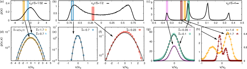
Figure 3: Velocity distributions. Panels (a), (b) and (c): density distribution $\rho(x)$ for $S=32,2,0.25$, respectively. Colored rectangles are drawn in correspondence of the spatial regions used to calculate the velocity distribution in the other panels. Panels (d), (e), (f), (g) and (h): distribution $p(v,x)$ as a function of $v$ calculated at fixed positions $x$. Panel (d) is calculated at $S=32$, panels (e) and (f) at $S=2$ and panels (g) and (h) at $S=0.25$. Colored points are obtained by numerical simulations while solid black lines by plotting the theoretical prediction (9). Simulations are realized with $\tau k/\gamma=1$ and $\alpha=0.9$.

IV.2 Velocity distribution

We now focus on the dependence of the full joint probability density $p(x,v)$ on the velocity, shown in Fig. 3 for some representative values of the particle’s position $x$. Moreover, we choose three different values of $S/(v_{0}\tau)$ to explore the three distinct regimes observed in Sec IV.1. For each regime, we report once again the density distribution $\rho(x)$ (panels (a), (b) and (c)), where colored bars mark the regions for which we calculate $p(x,v)$ as a function of $v$ in panels (d), (e), (f), (g), (h).

In the regime of small persistence, $(v_{0}\tau)/S\ll 1$, the shape of $p(v,x)$ is Gaussian, independently of the position $x$ (Fig. 3 (d)). This result fully agrees with the prediction (9) as revealed by the comparison between colored data points and black solid lines in Fig. 3 (d). As predicted by the space-dependent variance in Eq. (11), different positions $x$ come along with a change in the width of the velocity distribution.

In Fig. 3 (e) and (f), the regime of intermediate persistence, $v_{0}\tau/S\sim 1$, which displays a bimodality in the density distribution, is investigated. Here, we compare $p(x,v)$ calculated in the vicinity of a peak of $\rho(x)$ to the velocity profile near the local minimum of $\rho(x)$ (at the origin). In the former case, the distribution $p(x,v)$ displays an almost Gaussian shape in agreement with Eq. (3), while in the latter case, it deviates from the theoretical prediction and shows a non-Gaussian nature. In particular, the shape of $p(x,v)$ becomes asymmetric in $v$ and develops non-Gaussian tails. While the prediction (3) cannot account for non-Gaussianity, we remark that its quality near the regions where the particle preferably accumulates resembles the one obtained in Ref. Caprini et al. (2019a), where an AOUP (with $u(x)=v_{0}$) has been studied in a single-well anharmonic confinement.

Finally, the large-persistence regime, $v_{0}\tau/S\gg 1$, where the density distribution has multiple peaks also gives rise to a rich phenomenology of the stationary velocity profile, as shown in Fig. 3 (g) and (h). In the spatial regions for which $\Lambda(x)>0$, i.e., where the particles accumulate, the velocity distribution $p(x,v)$ (at fixed $x$) is described by the Gaussian distribution with space-dependent variance given by Eq. (3) (see Fig. 3 (g)), as in the case $v_{0}\tau/S\lesssim 1$. Instead, in the spatial regions where $\Lambda(x)<0$, i.e., between the primary and the secondary peaks (see also Fig. 2 (c)), the distribution displays a non-Gaussian shape (see Fig. 3 (h)). Compared to the case $v_{0}\tau/S\sim 1$, the non-Gaussianity is much more evident due to the occurrence of a bimodal behavior in the velocity distribution. In more detail, upon shifting the position $x$ in the $p(x,v)$ closer to the origin (Fig. 3 (g) and (h)), we observe that, starting from a nearly Gaussian shape centered at $v=0$ (pink curve), the main peak moves toward $v<0$ and a second small peak starts growing for $v>0$ (brown curve). Shifting again $x$, the second peak becomes dominant (yellow curve) and moves closer toward $v=0$ until the distribution is again described by a Gaussian (green curve). This phenomenology resembles the one observed in the case of an AOUP with $u(x)=v_{0}$ in a double-well potential Caprini et al. (2019c). Also in the latter case, the velocity distribution at fixed position exhibits bimodality in the spatial regions where the effective friction coefficient $\Lambda(x)\simeq\Gamma(x)$ becomes negative, although this effect is then induced by the negative curvature of the potential.

IV.3 Spatial profile of the kinetic temperature

Figure 4: Spatial profile of the kinetic temperature. $\langle v^{2}(x)\rangle$ as a function of $x$ for different values of the dimensionless parameter $v_{0}\tau/S$ at fixed $\tau k/\gamma$ and $\alpha$. Panel (a) shows the small-persistence regime, $v_{0}\tau/S\leq 1$, while panel (b) displays the intermediate-persistence and large-persistence regimes, namely $v_{0}\tau/S\sim 1$ and $v_{0}\tau/S\geq 1$, respectively. Colored points are obtained from numerical simulations while solid colored lines from the theoretical prediction (11). Simulations are realized with $\tau k/\gamma=1$ and $\alpha=0.9$.

To emphasize the dynamical effects due to the spatial modulation of the swim velocity, we focus on the profile of the kinetic temperature defined as the variance of the particle velocity, $\langle v^{2}(x)\rangle$. We show $\langle v^{2}(x)\rangle$ as a function of $x$ in Fig. 4 for values of $v_{0}\tau/S$ spanning all regimes from small (panel (a)) to intermediate and large persistence (panel (b)).

For small values of $v_{0}\tau/S\ll 1$, the profile $\langle v^{2}(x)\rangle$ is rather flat and attains its maximum value at $x=0$, i.e., the position of the potential minimum (see Fig. 4 (a)). When $v_{0}\tau/S$ increases, e.g., due to a shorter periodicity $S$ of the swim-velocity $u(x)$, the variance of the particle velocity becomes steeper and decreases to zero in the regions which are not explored by the particle. This is consistent with the scenario observed in Fig. 1 (c): the particles accumulate in the regions where they move slowly and the velocity variance is small. Such a result agrees with the observed behavior in the potential-free case (such that $u(x)$ coincides the particle velocity), where the particles accumulate in regions corresponding to the minima of $u(x)$, according to the law $\rho(x)\sim 1/u(x)$. In this regime, the comparison between numerical data and the theoretical prediction (11) (with $\Lambda(x)$ given by Eq. (19)) shows a good agreement.

For larger values of $v_{0}\tau/S$ (large-persistence regime), the velocity variance shows a more complex profile (see Fig. 4 (b)), which resembles the oscillating shape of $u(x)$. In particular, $\langle v^{2}(x)\rangle$ is very small near the peaks of the density distribution, while assumes larger values in the regions where the density is very small and the probability of finding a particle is very low. This finding is consistent with the fact that active particles accumulate in the regions where the velocity variance is small. Finally, in this regime, the prediction (11) reproduces quite well the behavior near the origin but fails further away from it, specifically, in the regions where the effective friction displays negative values, $\Lambda(x)<0$.

V Conclusion

In this paper, we have investigated the stationary behavior of an active particle subject to two competing spatial-dependent drivings: the self-propulsion velocity and the external force. While the two mechanisms were already investigated separately, to the best of our knowledge, this is the first time that their interplay has been considered. Starting from a Fokker-Planck description of the particle’s dynamics in our generalized AOUP model Caprini and Marconi (2021), we have developed a theoretical treatment, applicable to rather general choices of confining potentials and inhomogeneous swim velocities which provides the steady-state distribution (9) of both positions and velocities as a function of the input potential and of the swim velocity profile. The theory presented here contains as special cases both the UCNA describing the time evolution of distribution of positions and velocities of an AOUP with constant swim velocity in an external field Maggi et al. (2015b); Marconi et al. (2017), and the recent theory of a free AOUP driven by an inhomogeneous propulsion force, which is exact in the stationary case Caprini et al. (2022b). Our theoretical method is exact in the small-persistence regime, being consistent with the results obtained through an exact perturbative method, and also provides a useful approximation to qualitatively predict the shape of the distributions in the large-persistence regime.

Specifically, we have applied our theory to an AOUP in a sinusoidal motility landscape subject to a harmonic potential. We corroborated all theoretical predictions by numerical simulations and found a good agreement. The system revealed an intriguing scenario determined by the joint action of the self-propulsion velocity gradient and the external force. While, in the regime of small persistence, both the density and the velocity distributions are bell shaped and well-approximated by Gaussians, we predict that, as the persistence length becomes comparable with the spatial period of the swim velocity, a transition from a unimodal to a bimodal density occurs, also accompanied by a strong non-Gaussian effects in the velocity distribution. Interestingly, in the large-persistence regime, as the density shows multi-modality, the velocity distribution becomes bimodal in the spatial regions between two successive peaks of the density.

Moreover, we have shown that the interplay between the external force and the modulation of the swim velocity can be used to manipulate the behavior of a confined active particle, for instance by locally increasing the kinetic temperature or by forcing the particles to accumulate in distinct spatial regions with different probability. This possibility to fine-tune the steady-properties of active particles opens up a new avenue for future applications and developments. While, for active colloids, the emergence of an additional effective torque due to the spatial modulation of the swim velocity could be responsible for an even more complex phenomenology Lozano et al. (2016); Jahanshahi et al. (2020), we outline that our theory should be suitable in the case of engineered bacteria whose velocity profile can be manipulated by external light Arlt et al. (2018); Frangipane et al. (2018). From a pure theoretical perspective, our techniques may also be extended and applied to more complex dynamics, for instance accounting for the presence of thermal noise, a space-dependent torque Lozano et al. (2016); Jahanshahi et al. (2020), or additional competing nonconservative force fields like a Lorentz force Vuijk et al. (2020). A final challenging research point concerns the dynamical properties of our model and, in particular, the extension of the theory to time-dependent swim velocity profiles $u(x,t)$, for instance in the form of traveling waves Lozano et al. (2019); Koumakis et al. (2019); Geiseler et al. (2017b).

Appendix A Derivation of the auxiliary dynamics (6)

To derive the auxiliary dynamics (6), we start from Eq. (2a) chosing $D_{\text{t}}=0$. We recall that following Ref. Caprini and Marconi (2018) it is possible to generalize the procedure also to include the more general case with $D_{\text{t}}>0$. At first, we take the time-derivative of Eq. (2a), obtaining:

$$\gamma\ddot{\mathbf{x}}=-\nabla\nabla U\cdot\dot{\mathbf{x}}+\gamma\bm{\eta}\left(\frac{\partial}{\partial t}+\mathbf{v}\cdot\nabla\right)u(\mathbf{x},t)+\gamma u(\mathbf{x},t)\dot{\bm{\eta}}\,.$$ (22)

By defining the $\mathbf{v}=\dot{\mathbf{x}}$ as the particle velocity and replacing $\dot{\mathbf{f}}_{a}$ with the dynamics (2b), we get:

$$\gamma\dot{\mathbf{v}}= -\nabla\nabla U\cdot{\mathbf{v}}+\gamma\bm{\eta}\left(\frac{\partial}{\partial t}+\mathbf{v}\cdot\nabla\right)u(\mathbf{x},t)+\gamma u(\mathbf{x},t)\left(-\frac{\bm{\eta}}{\tau}+\frac{\sqrt{2}}{\sqrt{\tau}}\bm{\chi}\right)\,.$$ (23)

Finally, by replacing $\bm{\eta}$ in favor of $\mathbf{v}$ and $\mathbf{x}$, taking advantage of the relation (2a), we obtain the dynamics (6).

Appendix B Derivation of predictions (9) and (10)

To predict the shape of the stationary probability distributions, $p(\mathbf{x},\mathbf{v})$ and $\rho(\mathbf{x})$, stated in Sec. III, we start from the dynamics in the variables $\mathbf{x}$ and $\mathbf{v}$, namely Eq. (6), for a static profile of the swim velocity, $u(\mathbf{x})$. Switching to the Fokker-Planck equation for $p=p(\mathbf{x},\mathbf{v},t)$, we obtain:

$$\partial_{t}p= \nabla_{v}\cdot\left(\frac{\bm{\Gamma}}{\tau}\cdot\mathbf{v}p+\frac{u^{2}(\mathbf{x})}{\tau}\nabla_{v}p\right)-\mathbf{v}\cdot\nabla p+\nabla\cdot\frac{\nabla U}{\gamma\tau}p-\nabla_{v}\cdot\frac{\left[\gamma\mathbf{v}+\nabla U\right]}{\gamma u(\mathbf{x})}\left(\mathbf{v}\cdot\nabla\right)u(\mathbf{x})\,,$$ (24)

where $\nabla$ and $\nabla_{v}$ are the vectorial derivative operators in position and velocity space, respectively. Balancing the diffusion term (proportional to the Laplacian of $\mathbf{v}$) and the other effective friction terms (say the one linearly proportional to $\mathbf{v}$), we get the condition:

$$0=\nabla_{v}\cdot\left(\frac{\bm{\Lambda}}{\tau}\cdot\mathbf{v}p+\frac{u^{2}(\mathbf{x})}{\tau}\nabla_{v}p\right)\,$$ (25)

with the effective friction matrix

$$\bm{\Lambda}(\mathbf{x})=\bm{\text{I}}+\frac{\tau}{\gamma}\nabla\nabla U(\mathbf{x})-\frac{\tau}{\gamma}\nabla U(\mathbf{x})\frac{\nabla u(\mathbf{x})}{u(\mathbf{x})}\,,$$ (26)

that has been defined in Eq. (8). The condition (25) corresponds of requiring that all the irreversible currents are zero, in the same spirit of Ref. Marconi et al. (2017). The solution of Eq. (25) corresponds to Eq. (9), where $\rho(\mathbf{x})$ is still an unknown function to be determined below.

To determine the function $\rho(\mathbf{x})$, we first identify the acceleration term Jung and Hänggi (1988)

$$u(\mathbf{x})\frac{d}{dt}\frac{\mathbf{v}}{u(\mathbf{x})}=\dot{\mathbf{v}}-\frac{\mathbf{v}}{u(\mathbf{x},t)}\left(\mathbf{v}\cdot\nabla\right)u(\mathbf{x},t)\,$$ (27)

in the dynamics (6). Assuming that the velocity relaxes faster than the position allows us to neglect both these terms in Eq. (6), obtaining the following overdamped equation:

$$\dot{\mathbf{x}}=-\frac{1}{\gamma}\bm{\Lambda}^{-1}\cdot\nabla U+\sqrt{2\tau}u(\mathbf{x})\bm{\Lambda}^{-1}\cdot\bm{\chi}\,.$$ (28)

From this dynamics, it is convenient to switch to the effective Smoluchowski equation for the density of the system, $\rho(\mathbf{x},t)$, and use the Stratonovich convention, obtaining:

$$\frac{\partial\rho}{\partial t}=\frac{\partial}{\partial x_{i}}\left(\frac{1}{\gamma}\Lambda^{-1}_{ij}\left(\frac{\partial U}{\partial x_{j}}\right)\,\rho+\tau u\Lambda^{-1}_{ik}\frac{\partial}{\partial x_{j}}\left[\Lambda^{-1}_{jk}u\rho\right]\right)\,.$$ (29)

Here and in what follows, we have explicitly written Latin indices for the spatial components of vectors and matrices and adopted also the Einstein’s convention for repeated indices, for convenience.

To proceed, we assume the zero-current condition, obtaining an effective equation for the stationary density $\rho(\mathbf{x})$:

$$\frac{1}{\gamma}\Lambda^{-1}_{ij}\left(\frac{\partial U}{\partial x_{j}}\right)\,\rho+\tau u\Lambda^{-1}_{ik}\frac{\partial}{\partial x_{j}}\left[\Lambda^{-1}_{jk}u\rho\right]=0\,.$$ (30)

Multiplying by $\Lambda_{lh}\Lambda_{hi}$ and summing over repeated indices, we get the following relation after some algebraic manipulations

$$\frac{1}{\gamma\tau u^{2}}\Lambda_{lj}\frac{\partial U}{\partial x_{j}}+\Lambda_{lk}\frac{\partial}{\partial x_{j}}\Lambda^{-1}_{jk}+\frac{\Lambda_{lk}\Lambda^{-1}_{jk}}{u\rho}\frac{\partial}{\partial x_{j}}[u\rho]=0\,,$$ (31)

whose solution for the density distribution $\rho(\mathbf{x})$ reads:

$$\rho(\mathbf{x})\approx\frac{\mathcal{N}}{u(\mathbf{x})}\exp{\Biggl{(}\frac{1}{\gamma\tau}\int^{x}d\mathbf{y}\cdot\frac{\bm{\Lambda}(\mathbf{y})\cdot\mathbf{F}(\mathbf{y})}{u^{2}(\mathbf{y})}+\int^{x}d\mathbf{y}\cdot\bm{\Lambda}(\mathbf{y})\cdot\nabla\cdot\bm{\Lambda}^{-1}(\mathbf{y})\Biggr{)}}\,.$$ (32)

Finally, by assuming a planar symmetry for both $u$ and $U$, we have $\nabla\cdot\bm{\Lambda}^{-1}\equiv\hat{e}_{x}\cdot\partial\bm{\Lambda}^{-1}/\partial x$, where $\hat{e}_{x}$ denotes the unit vector corresponding to the coordinate $x$, and can therefore use the explicit Jacobi relation

$$\bm{\Lambda}\cdot\hat{e}_{x}\cdot\frac{\partial\bm{\Lambda}^{-1}}{\partial x}=-\frac{1}{\det[\bm{\Lambda}]}\hat{e}_{x}\frac{\partial\det[\bm{\Lambda}]}{\partial x}=-\hat{e}_{x}\frac{\partial\ln\det[\bm{\Lambda}]}{\partial x}$$ (33)

for the determinant $\det\bm{\Lambda}$ of a matrix $\bm{\Lambda}$. We remark that the general relation

$$\bm{\Lambda}\cdot\nabla\cdot\bm{\Lambda}^{-1}=-\nabla\ln\det[\bm{\Lambda}]$$ (34)

only holds in the above planar case (33) or for a constant swim velocity $u(\bm{x})=v_{0}$, see also appendix B of Ref. Wittmann et al. (2017). However, since there are no conceptual differences, we can plug the approximation (34) into the prediction (32) to obtain the compact representation (10) of $\rho(\bm{x})$ in the main text.

The same stationary condition (31) can be obtained using the Fox approach Fox (1986b) (when generalized to multiple components Rein and Speck (2016); Sharma et al. (2017)), while the corresponding time evolution differs from the UCNA dynamics (29) by the additional occurrence of the factors $\Lambda^{-1}_{ij}$ and $\Lambda^{-1}_{ik}$ therein. Note that, if we do not neglect the thermal Brownian noise in Eq. (2), also the stationary predictions of Fox and UCNA differ, even for a spatially constant swim velocity Wittmann et al. (2017).

Appendix C Multi-scale technique: derivation of Eq. (14)

In this appendix, we derive the perturbative result (14) for the probability distribution $p(x,v)$ in the one-dimensional active system described by the Fokker-Planck equation (13). We adopt the multiple-time-scale technique, which is designed to deal with problems with fast and slow degrees of freedom. In the regime of small persistence time (where $\tau$ is the smallest time scale of the system), the dynamics (13) exhibits the separation of time scales: in this case, the particle velocity rapidly arranges according to its stationary distribution and the spatial distribution evolves on a slower time scale.

To derive the multiple-time expansion, let us introduce the following dimensionless variables:

$$\tilde{t}=t\frac{v_{0}}{S}\,,$$ (35)

$$X=\frac{x}{S}\,,$$ (36)

$$V=\frac{v}{v_{0}}\,,$$ (37)

$$\tilde{F}(X)=-\frac{S}{v_{0}^{2}\tau\gamma}\frac{\partial U(x)}{\partial x}\,,$$ (38)

$$\tilde{\Gamma}(X)=1-\tau^{2}\frac{v_{0}^{2}}{S^{2}}\frac{\partial\tilde{F}(X)}{\partial X}\,,$$ (39)

$$w(X)=\frac{u(x)}{v_{0}}\,,$$ (40)

and the small expansion parameter $\zeta^{-1}\propto\tau$, where

$$\zeta=\frac{S}{\tau v_{0}}\,$$ (41)

is the ratio between the spatial period of the swim velocity $S$ and the persistence length of the self-propulsion velocity $v_{0}\tau$. With our choice, a large (small) value of $\zeta$ corresponds to the small-persistence (large-persistence) regime. Now, we express the Fokker-Planck equation (13) in these variables and find:

$$\frac{\partial P(X,V,\bar{t})}{\partial\bar{t}}+V\frac{\partial}{\partial X}P+\tilde{F}(X)\frac{\partial}{\partial V}P+\frac{1}{\zeta}R(X)\frac{\partial}{\partial V}VP$$

$$+\frac{1}{w(X)}\frac{\partial}{\partial X}w(X)\frac{\partial}{\partial V}(V^{2}P)=\zeta L_{\text{FP}}P\,,$$ (42)

where we have further introduced the operator

$$L_{\text{FP}}\equiv\frac{\partial}{\partial V}\Bigl{(}V+w^{2}(X)\frac{\partial}{\partial V}\Bigr{)}$$ (43)

and the function

$$R(X)\equiv\Bigl{[}\frac{\partial\tilde{F}}{\partial X}-\tilde{F}(X)\frac{1}{w(X)}\frac{\partial}{\partial X}w(X)\Bigr{]}\,,$$ (44)

for convenience.

To develop our perturbative solution, we notice that the local operator $L_{\text{FP}}$ is proportional to the inverse expansion parameter $\zeta$ in Eq. (42). We find that $L_{\text{FP}}$ has the following integer eigenvalues:

$$\nu=0,-1,-2,\ldots$$ (45)

and the Hermite polynomials as eigenfunctions:

$$H_{\nu}(X,V)=\frac{(-1)^{\nu}}{\sqrt{2\pi}}\left(w(X)\right)^{(\nu-1)}\frac{\partial^{\nu}}{\partial V^{\nu}}\,e^{-\frac{V^{2}}{2w^{2}(X)}}\,.$$ (46)

Using these basis functions, we obtain the ansatz to write the solution of the partial differential equation as a linear combination:

$$P(X,V,\tilde{t})=\sum_{\nu=0}^{\infty}\phi_{\nu}(X,\tilde{t})H_{\nu}(X,V)\,.$$ (47)

Upon substituting the expansion (47) in Eq. (42) and replacing $L_{\text{FP}}$ by its eigenvalues, we obtain the equation:

$$-\zeta\sum_{\nu}\nu\,\phi_{\nu}H_{\nu}=\sum_{\nu}\frac{\partial\phi_{\nu}}{\partial\tilde{t}}H_{\nu}$$

$$+\sum_{\nu}VH_{\nu}\frac{\partial}{\partial X}\phi_{\nu}+\sum_{\nu}\phi_{\nu}V\frac{\partial}{\partial X}H_{\nu}+\tilde{F}\sum_{\nu}\phi_{\nu}\frac{\partial}{\partial V}H_{\nu}$$

$$+\frac{w^{\prime}}{w}\sum_{\nu}\phi_{\nu}\frac{\partial}{\partial V}V^{2}H_{\nu}+\frac{1}{\zeta}R\sum_{\nu}\phi_{\nu}\frac{\partial}{\partial V}VH_{\nu}\,,$$ (48)

from which we must determine the unknown functions $\phi_{\nu}(x,t)$.

Now, instead of truncating arbitrarily the infinite series in Eq. (48) at some order $\nu$, we consider the multiple-time expansion which orders the series in powers of the small parameter $1/\zeta$. In such a way we perform an expansion near the equilibrium solution. To this end, each amplitude $\phi_{\nu}$ (apart from $\phi_{0}(X,\tilde{t})$ which is of order $\zeta^{0}$) is expanded in powers of $1/\zeta$ as:

$$\phi_{\nu}(X,\tilde{t})=\sum_{s=0}^{\infty}\frac{1}{\zeta^{s}}\psi_{s\nu}(X,\tilde{t})\,.$$ (49)

Then, we replace the actual distribution $P(X,V,\bar{t})$ by an auxiliary distribution $P_{a}=P_{a}(X,V,\bar{t}_{0},\bar{t}_{1},\bar{t}_{2},..)$, which reads:

$$P_{a}=\sum_{s=0}^{\infty}\frac{1}{\zeta^{s}}\sum_{\nu=0}^{\infty}\psi_{s\nu}(X,\bar{t}_{0},\bar{t}_{1},\bar{t}_{2},..)H_{\nu}(X,V)\,.$$ (50)

This distribution depends on many time variables $\{\bar{t}_{s}\}$, associated with the perturbation order $s$, which are defined as $\bar{t}_{s}=\bar{t}/\zeta^{s}$. The time derivative with respect to $\bar{t}$ is then expressed as the sum of partial time-like derivatives:

$$\frac{\partial}{\partial\bar{t}}=\frac{\partial}{\partial\bar{t}_{0}}+\frac{1}{\zeta}\frac{\partial}{\partial\bar{t}_{1}}+\frac{1}{\zeta^{2}}\frac{\partial}{\partial\bar{t}_{2}}+\ldots\,.$$ (51)

Substituting the expansions (49) and (51) into Eq. (48) one obtains at each order $1/\zeta^{s}$ and for each Hermite function an equation involving the amplitudes $\psi_{s\nu}(X,\tilde{t})$. The perturbative structure of the resulting set of equations is such that the amplitudes $\psi_{s\nu}(X,\tilde{t})$ can be obtained by the amplitudes of the lower order $(s-1)$. In particular, we find the following equation for $\psi_{00}=\phi_{0}$

$$\frac{\partial\psi_{00}(X,\bar{t})}{\partial\tilde{t}}=\frac{1}{\zeta}\frac{\partial}{\partial X}\Bigl{[}w(X)\frac{\partial}{\partial X}\Bigl{(}w(X)\psi_{00}\Bigr{)}$$

$$-\tilde{F}(X)\psi_{00}+\frac{1}{\zeta^{2}}w(X)\frac{\partial}{\partial X}\Bigl{(}w(X)R\psi_{00}\Bigr{)}\Bigr{]}\,,$$ (52)

whose steady-state solution reads

$$\psi_{00}(X)= \frac{\mathcal{N}}{w(X)}\,\Bigl{(}1-\frac{1}{\zeta^{2}}R(X)\Bigr{)}\times\exp\left[\int^{X}dy\frac{\tilde{F}(y)}{w^{2}(y)}\Bigl{(}1-\frac{1}{\zeta^{2}}R(y)\Bigr{)}\right]\,,$$ (53)

where $\mathcal{N}$ is a normalization factor. In our perturbative procedure, all the remaining amplitudes are expressed in terms of the pivot function $\psi_{00}(X)$. The steady-state amplitudes of the higher-order Hermite polynomials are given by:

$$\psi_{22}=\frac{1}{2}R(X)\psi_{00}$$ (54)

$$\psi_{33}(X)=-\frac{1}{6}w(X)\psi_{00}(X)\frac{\partial}{\partial X}R(X)$$ (55)

$$\psi_{42}=-\frac{3}{2}\frac{\partial}{\partial X}[w(X)\psi_{33}]+R(X)\psi_{22}$$ (56)

$$\psi_{44}(X)=-\frac{1}{4}\Bigl{(}\frac{\partial}{\partial X}[w(X)\psi_{33}]-R(X)\psi_{22}\Bigr{)}\,,$$ (57)

where we have reported only the nonvanishing coefficients for $s\leq 4$. Note that, if $\nu>s$, the coefficients $\psi_{s\nu}$ are always zero.

Once Eq. (53) and the coefficients of the double series (50) have been determined, one returns to the original dimensional variables and obtains the perturbative result for $p(x,v)$ reported in Eq. (14).

References

- Bechinger et al. (2016) C. Bechinger, R. Di Leonardo, H. Löwen, C. Reichhardt, G. Volpe, and G. Volpe, Reviews of Modern Physics 88, 045006 (2016).
- Marchetti et al. (2013) M. Marchetti, J. Joanny, S. Ramaswamy, T. Liverpool, J. Prost, M. Rao, and R. A. Simha, Reviews of Modern Physics 85, 1143 (2013).
- Elgeti et al. (2015) J. Elgeti, R. G. Winkler, and G. Gompper, Reports on Progress in Physics 78, 056601 (2015).
- Gompper et al. (2020) G. Gompper, R. G. Winkler, T. Speck, A. Solon, C. Nardini, F. Peruani, H. Löwen, R. Golestanian, U. B. Kaupp, L. Alvarez, et al., Journal of Physics: Condensed Matter 32, 193001 (2020).
- Lavergne et al. (2019) F. A. Lavergne, H. Wendehenne, T. Bäuerle, and C. Bechinger, Science 364, 70 (2019).
- Sprenger et al. (2020) A. R. Sprenger, M. A. Fernandez-Rodriguez, L. Alvarez, L. Isa, R. Wittkowski, and H. Löwen, Langmuir 36, 7066 (2020).
- Fernandez-Rodriguez et al. (2020) M. A. Fernandez-Rodriguez, F. Grillo, L. Alvarez, M. Rathlef, I. Buttinoni, G. Volpe, and L. Isa, Nature communications 11, 1 (2020).
- Fränzl and Cichos (2020) M. Fränzl and F. Cichos, Scientific reports 10, 1 (2020).
- Walter et al. (2007) J. M. Walter, D. Greenfield, C. Bustamante, and J. Liphardt, Proceedings of the National Academy of Sciences 104, 2408 (2007).
- Buttinoni et al. (2012) I. Buttinoni, G. Volpe, F. Kümmel, G. Volpe, and C. Bechinger, Journal of Physics: Condensed Matter 24, 284129 (2012).
- Palacci et al. (2013) J. Palacci, S. Sacanna, A. P. Steinberg, D. J. Pine, and P. M. Chaikin, Science 339, 936 (2013).
- Dai et al. (2016) B. Dai, J. Wang, Z. Xiong, X. Zhan, W. Dai, C.-C. Li, S.-P. Feng, and J. Tang, Nature Nanotechnology 11, 1087 (2016).
- Li et al. (2016) W. Li, X. Wu, H. Qin, Z. Zhao, and H. Liu, Advanced Functional Materials 26, 3164 (2016).
- Uspal (2019) W. Uspal, The Journal of Chemical Physics 150, 114903 (2019).
- Bregulla et al. (2014) A. P. Bregulla, H. Yang, and F. Cichos, Acs Nano 8, 6542 (2014).
- Jahanshahi et al. (2020) S. Jahanshahi, C. Lozano, B. Liebchen, H. Löwen, and C. Bechinger, Communications Physics 3, 1 (2020).
- Söker et al. (2021) N. A. Söker, S. Auschra, V. Holubec, K. Kroy, and F. Cichos, Physical Review Letters 126, 228001 (2021).
- Auschra and Holubec (2021) S. Auschra and V. Holubec, Physical Review E 103, 062604 (2021).
- Lozano et al. (2016) C. Lozano, B. Ten Hagen, H. Löwen, and C. Bechinger, Nature Communications 7, 12828 (2016).
- Maggi et al. (2015a) C. Maggi, F. Saglimbeni, M. Dipalo, F. De Angelis, and R. Di Leonardo, Nature Communications 6, 7855 (2015a).
- Vizsnyiczai et al. (2017) G. Vizsnyiczai, G. Frangipane, C. Maggi, F. Saglimbeni, S. Bianchi, and R. Di Leonardo, Nature Communications 8, 15974 (2017).
- Stenhammar et al. (2016) J. Stenhammar, R. Wittkowski, D. Marenduzzo, and M. E. Cates, Science Advances 2, e1501850 (2016).
- Koumakis et al. (2019) N. Koumakis, A. T. Brown, J. Arlt, S. E. Griffiths, V. A. Martinez, and W. C. Poon, Soft Matter 15, 7026 (2019).
- Lozano et al. (2019) C. Lozano, B. Liebchen, B. Ten Hagen, C. Bechinger, and H. Löwen, Soft Matter 15, 5185 (2019).
- Arlt et al. (2018) J. Arlt, V. A. Martinez, A. Dawson, T. Pilizota, and W. C. K. Poon, Nature Communications 9, 768 (2018).
- Arlt et al. (2019) J. Arlt, V. A. Martinez, A. Dawson, T. Pilizota, and W. C. Poon, Nature Communications 10, 2321 (2019).
- Frangipane et al. (2018) G. Frangipane, D. Dell’Arciprete, S. Petracchini, C. Maggi, F. Saglimbeni, S. Bianchi, G. Vizsnyiczai, M. L. Bernardini, and R. Di Leonardo, Elife 7, e36608 (2018).
- Schnitzer (1993) M. J. Schnitzer, Physical Review E 48, 2553 (1993).
- Tailleur and Cates (2008) J. Tailleur and M. Cates, Physical Review Letters 100, 218103 (2008).
- Sharma and Brader (2017) A. Sharma and J. M. Brader, Physical Review E 96, 032604 (2017).
- Ghosh et al. (2015) P. K. Ghosh, Y. Li, F. Marchesoni, and F. Nori, Physical Review E 92, 012114 (2015).
- Liebchen and Löwen (2019) B. Liebchen and H. Löwen, EPL (Europhysics Letters) 127, 34003 (2019).
- Fischer et al. (2020) A. Fischer, F. Schmid, and T. Speck, Physical Review E 101, 012601 (2020).
- Bäuerle et al. (2018) T. Bäuerle, A. Fischer, T. Speck, and C. Bechinger, Nature Communications 9, 3232 (2018).
- Jose et al. (2021) F. Jose, S. K. Anand, and S. P. Singh, Soft Matter 17, 3153 (2021).
- Azimi et al. (2020) S. Azimi, A. D. Klementiev, M. Whiteley, and S. P. Diggle, Annual Review of Microbiology 74, 201 (2020).
- Vuijk et al. (2018) H. D. Vuijk, A. Sharma, D. Mondal, J.-U. Sommer, and H. Merlitz, Physical Review E 97, 042612 (2018), URL https://link.aps.org/doi/10.1103/PhysRevE.97.042612.
- Merlitz et al. (2020) H. Merlitz, H. D. Vuijk, R. Wittmann, A. Sharma, and J.-U. Sommer, PLOS ONE 15, 1 (2020), URL https://doi.org/10.1371/journal.pone.0230873.
- Richard Lapidus (1980) I. Richard Lapidus, Journal of Theoretical Biology 86, 91 (1980), ISSN 0022-5193, URL https://www.sciencedirect.com/science/article/pii/0022519380900673.
- Vuijk et al. (2021) H. D. Vuijk, H. Merlitz, M. Lang, A. Sharma, and J.-U. Sommer, Physical Review Letter 126, 208102 (2021), URL https://link.aps.org/doi/10.1103/PhysRevLett.126.208102.
- Grauer et al. (2018) J. Grauer, H. Löwen, and L. M. Janssen, Physical Review E 97, 022608 (2018).
- Magiera and Brendel (2015) M. P. Magiera and L. Brendel, Physical Review E 92, 012304 (2015).
- Maggi et al. (2018) C. Maggi, L. Angelani, G. Frangipane, and R. Di Leonardo, Soft Matter 14, 4958 (2018).
- Merlitz et al. (2018) H. Merlitz, H. D. Vuijk, J. Brader, A. Sharma, and J.-U. Sommer, The Journal of Chemical Physics 148, 194116 (2018).
- Lozano and Bechinger (2019) C. Lozano and C. Bechinger, Nature Communications 10, 2495 (2019).
- Geiseler et al. (2017a) A. Geiseler, P. Hänggi, and F. Marchesoni, Entropy 19, 97 (2017a).
- Zampetaki et al. (2019) A. Zampetaki, P. Schmelcher, H. Löwen, and B. Liebchen, New Journal of Physics 21, 013023 (2019).
- Zhu et al. (2018) W.-j. Zhu, X.-q. Huang, and B.-q. Ai, Journal of Physics A: Mathematical and Theoretical 51, 115101 (2018).
- Geiseler et al. (2017b) A. Geiseler, P. Hänggi, and F. Marchesoni, Scientific Reports 7, 41884 (2017b).
- Solon et al. (2015) A. P. Solon, J. Stenhammar, R. Wittkowski, M. Kardar, Y. Kafri, M. E. Cates, and J. Tailleur, Physical Review Letters 114, 198301 (2015).
- Flenner et al. (2016) E. Flenner, G. Szamel, and L. Berthier, Soft matter 12, 7136 (2016).
- Petrelli et al. (2018) I. Petrelli, P. Digregorio, L. F. Cugliandolo, G. Gonnella, and A. Suma, The European Physical Journal E 41, 128 (2018).
- Caprini and Marconi (2021) L. Caprini and U. M. B. Marconi, Soft Matter 17, 4109 (2021).
- Negro et al. (2022) G. Negro, C. B. Caporusso, P. Digregorio, G. Gonnella, A. Lamura, and A. Suma, arXiv preprint arXiv:2201.10019 (2022).
- Chacon et al. (2022) E. Chacon, F. Alarcón, J. Ramirez, P. Tarazona, and C. Valeriani, Soft Matter (2022).
- Caprini et al. (2022a) L. Caprini, A. R. Sprenger, H. Löwen, and R. Wittmann, The Journal of Chemical Physics 156, 071102 (2022a).
- Maggi et al. (2015b) C. Maggi, U. M. B. Marconi, N. Gnan, and R. Di Leonardo, Scientific Reports 5, 10742 (2015b).
- Szamel (2014) G. Szamel, Physical Review E 90, 012111 (2014).
- Dabelow et al. (2019) L. Dabelow, S. Bo, and R. Eichhorn, Physical Review X 9, 021009 (2019).
- Berthier et al. (2019) L. Berthier, E. Flenner, and G. Szamel, The Journal of Chemical Physics 150, 200901 (2019).
- Martin et al. (2021) D. Martin, J. O’Byrne, M. E. Cates, É. Fodor, C. Nardini, J. Tailleur, and F. van Wijland, Physical Review E 103, 032607 (2021).
- Caprini and Marini Bettolo Marconi (2021) L. Caprini and U. Marini Bettolo Marconi, The Journal of Chemical Physics 154, 024902 (2021).
- Nguyen et al. (2021) G. H. P. Nguyen, R. Wittmann, and H. Löwen, Journal of Physics: Condensed Matter 34, 035101 (2021).
- Fily and Marchetti (2012) Y. Fily and M. C. Marchetti, Physical Review Letter 108, 235702 (2012).
- Farage et al. (2015) T. F. Farage, P. Krinninger, and J. M. Brader, Physical Review E 91, 042310 (2015).
- Maggi et al. (2017) C. Maggi, M. Paoluzzi, L. Angelani, and R. Di Leonardo, Scientific Reports 7, 17588 (2017).
- Maes (2020) C. Maes, Physical Review Letters 125, 208001 (2020).
- Wittmann et al. (2017) R. Wittmann, C. Maggi, A. Sharma, A. Scacchi, J. M. Brader, and U. M. B. Marconi, Journal of Statistical Mechanics: Theory and Experiment 2017, 113207 (2017).
- foo (2022a) The common mapping between ABPs and AOUPs in spatial dimensions relates the persistence time and the active diffusion coefficient of the AOUP model to the rotational diffusivity and self-propulsion-velocity scale of the ABP model Wittmann et al. (2017). To ease the notation for the predictions of our generalized AOUP model, we follow the convention of Ref. Caprini et al. (2022b) and do not imply this mapping, simply setting , which gives the same physics. If one wishes to make explicit contact to the ABP model for , the last term in Eq. (2b) should be replaced by , such that the formulas subsequently derived for arbitrary spatial dimension should be interpreted by rescaling . (2022a).
- Caprini et al. (2022b) L. Caprini, U. M. B. Marconi, R. Wittmann, and H. Löwen, Soft Matter 18, 1412 (2022b).
- Caprini and Marconi (2018) L. Caprini and U. M. B. Marconi, Soft Matter 14, 9044 (2018).
- Jung and Hänggi (1987) P. Jung and P. Hänggi, Physical Review A 35, 4464 (1987).
- Jung and Hänggi (1988) P. Jung and P. Hänggi, J. Opt. Soc. Am. B 5, 979 (1988), URL http://opg.optica.org/josab/abstract.cfm?URI=josab-5-5-979.
- Hänggi and Jung (1995) P. Hänggi and P. Jung, Advances in Chemical Physics 89, 239 (1995).
- Fox (1986a) R. F. Fox, Physical Review A 33, 467 (1986a), URL https://link.aps.org/doi/10.1103/PhysRevA.33.467.
- Fox (1986b) R. F. Fox, Phys. Rev. A 34, 4525 (1986b).
- Marconi et al. (2016) U. M. B. Marconi, N. Gnan, M. Paoluzzi, C. Maggi, and R. Di Leonardo, Scientific Reports 6, 23297 (2016).
- Caprini and Marini Bettolo Marconi (2020) L. Caprini and U. Marini Bettolo Marconi, The Journal of Chemical Physics 153, 184901 (2020).
- Bocquet (1997) L. Bocquet, American Journal of Physics 65, 140 (1997).
- Marini-Bettolo-Marconi et al. (2007) U. Marini-Bettolo-Marconi, P. Tarazona, and F. Cecconi, The Journal of chemical physics 126, 164904 (2007).
- Titulaer (1978) U. M. Titulaer, Physica A: Statistical Mechanics and its Applications 91, 321 (1978).
- Fodor et al. (2016) É. Fodor, C. Nardini, M. E. Cates, J. Tailleur, P. Visco, and F. van Wijland, Physical Review Letters 117, 038103 (2016).
- Marconi et al. (2017) U. M. B. Marconi, A. Puglisi, and C. Maggi, Scientific Reports 7, 46496 (2017).
- Martin and de Pirey (2021) D. Martin and T. A. de Pirey, Journal of Statistical Mechanics: Theory and Experiment 2021, 043205 (2021).
- foo (2022b) Notice the slightly different role of the expansion parameter in Eq. (14) for our version of the AOUP model (2), in which we have eliminated the active diffusion coefficient in favor of an expression containing the explicit factor . (2022b).
- Caprini et al. (2019a) L. Caprini, U. M. B. Marconi, and A. Puglisi, Scientific Reports 9, 1386 (2019a).
- Breoni et al. (2022) D. Breoni, R. Blossey, and H. Löwen, Eur. Phys. J. E 45 (2022).
- Das et al. (2018) S. Das, G. Gompper, and R. G. Winkler, New Journal of Physics 20, 015001 (2018).
- Caprini et al. (2019b) L. Caprini, E. Hernández-García, C. López, and U. M. B. Marconi, Scientific Reports 9, 16687 (2019b).
- Dabelow et al. (2021) L. Dabelow, S. Bo, and R. Eichhorn, Journal of Statistical Mechanics: Theory and Experiment 2021, 033216 (2021).
- Caprini et al. (2019c) L. Caprini, U. Marini Bettolo Marconi, A. Puglisi, and A. Vulpiani, The Journal of Chemical Physics 150, 024902 (2019c).
- Schwarzendahl and Löwen (2021) F. J. Schwarzendahl and H. Löwen, arXiv preprint arXiv:2111.06109 (2021).
- Caprini et al. (2021) L. Caprini, F. Cecconi, and U. Marini Bettolo Marconi, The Journal of Chemical Physics 155, 234902 (2021).
- Woillez et al. (2019) E. Woillez, Y. Zhao, Y. Kafri, V. Lecomte, and J. Tailleur, Physical review letters 122, 258001 (2019).
- Fily (2019) Y. Fily, The Journal of Chemical Physics 150, 174906 (2019).
- Woillez et al. (2020a) E. Woillez, Y. Kafri, and N. S. Gov, Physical Review Letters 124, 118002 (2020a).
- Woillez et al. (2020b) E. Woillez, Y. Kafri, and V. Lecomte, Journal of Statistical Mechanics: Theory and Experiment 2020, 063204 (2020b).
- Vuijk et al. (2020) H. D. Vuijk, J.-U. Sommer, H. Merlitz, J. M. Brader, and A. Sharma, Physical Review Research 2, 013320 (2020).
- Rein and Speck (2016) M. Rein and T. Speck, The European Physical Journal E 39, 84 (2016), URL https://doi.org/10.1140/epje/i2016-16084-7.
- Sharma et al. (2017) A. Sharma, R. Wittmann, and J. M. Brader, Physical Review E 95, 012115 (2017), URL https://link.aps.org/doi/10.1103/PhysRevE.95.012115.