Experimental identification of the second-order non-Hermitian skin effect with physics-graph-informed machine learning

Abstract

Topological phases of matter are conventionally characterized by the bulk-boundary correspondence in Hermitian systems: The topological invariant of the bulk in $d$ dimensions corresponds to the number of $(d-1)$-dimensional boundary states. By extension, higher-order topological insulators reveal a bulk-edge-corner correspondence, such that $n$-th order topological phases feature $(d-n)$-dimensional boundary states. The advent of non-Hermitian topological systems sheds new light on the emergence of the non-Hermitian skin effect (NHSE) with an extensive number of boundary modes under open boundary conditions. Still, the higher-order NHSE remains largely unexplored, particularly in the experiment. We introduce an unsupervised approach – physics-graph-informed machine learning (PGIML) – to enhance the data mining ability of machine learning with limited domain knowledge. Through PGIML, we experimentally demonstrate the second-order NHSE in a two-dimensional non-Hermitian topolectrical circuit. The admittance spectra of the circuit exhibit an extensive number of corner skin modes and extreme sensitivity of the spectral flow to the boundary conditions. The violation of the conventional bulk-boundary correspondence in the second-order NHSE implies that modification of the topological band theory is inevitable in higher dimensional non-Hermitian systems.

Introduction

Conceptual theories about topological phases of matter are at the forefront of contemporary research. In Hermitian systems, the guiding principle of topological insulators (TIs) is the bulk-boundary correspondence, stating that the topological invariants of the bulk determine the number of gapless boundary modes [1, 2, 3]. With progress in research, higher-order TIs have revealed a novel bulk-edge-corner correspondence, where $n$-th order topological phases in $d$ dimensions feature $(d-n)$-dimensional boundary modes [4, 5, 6, 7, 8, 9, 10, 11, 12, 13, 14, 15, 16]. Building up on the categories of Hermitian systems, non-conservative systems without Hermiticity reveal a plethora of unconventional physical principles, phenomena, and applications. Among many others, this includes parity-time symmetry [17, 18, 19], exceptional points [20], exceptional Fermi arcs [21], sensing [22, 23], and lasing [24, 25]. Recently, the concept of non-Hermiticity has been intertwined with topological phases of matter [26, 27, 28, 29] to yield the non-Hermitian skin effect (NHSE) with an extensive number of boundary modes and the necessity to assess non-Hermitian topological properties beyond Bloch band theory [30, 31, 32].

Despite a fast-growing number of theoretical predictions for non-Hermitian topological systems [33, 34, 35, 36, 37, 38, 39, 40, 41, 42, 43, 44, 45], experimental explorations are still at an early stage [46, 47, 48, 49, 50]. To date, the first-order NHSE has been realized in photonic [51] and in circuitry [46, 47, 48] environments, whereas the experimental realization of the higher-order NHSE remains open. Although skin corner modes have been observed in very recent research [49, 50], the unique features of the higher-order NHSE need to be fully demonstrated, both the extensive number of boundary modes under open boundary conditions and the extreme sensitivity of the spectral flow to the boundary conditions. To analyze the spectral flow in higher dimensions, traditional methodologies are challenged by the large-scale data generated. The data size will grow exponentially with the dimension, and additional boundary conditions make it more difficult to analyze the outcome. Machine learning (ML) is a promising way to process large amounts of data [52, 53, 54]. The existing approaches, however, are unable to efficiently extract the crucial observables, in particular with a largely unexplored state of matter at hand. There is a pressing need for integrating fundamental physical laws and domain knowledge by teaching ML models the governing physical rules, which can, in turn, provide informative priors, i.e., theoretical constraints and inductive understanding of the observable features. To this end, physics-informed ML, using informative priors for the phenomenological description of the world, can be leveraged to improve the performance of the learning algorithm [55].

In this article, we report two significant advances: (i) The methodology of physics-graph-informed machine learning (PGIML) is introduced to enforce identification of an unrevealed physical phenomenon by integrating physical principles, graph visualization of features, and ML. The informative priors provided by PGIML enable an analysis that remains robust even in the presence of imperfect data (such as missing values, outliers, and noise) to make accurate and physically consistent predictions of phenomenological parameters. (ii) The second-order NHSE, characterized by skin corner modes and the violation of the conventional bulk-boundary correspondence, is realized in a two-dimensional (2D) non-Hermitian topoelectrical circuit. We achieve the first experimental demonstration of the extreme sensitivity of the spectral flow to (fully controlled) boundary conditions (PBC$x$-PBC$y$, PBC$x$-OBC$y$, OBC$x$-PBC$y$, and OBC$x$-OBC$y$, where PBC (OBC) represents a periodic (open) boundary condition and $x$ $(y)$ represents direction), and observe corner skin modes under OBC$x$-OBC$y$ as well as edge skin modes under PBC$x$-OBC$y$. Prospectively, the powerful tool of PGIML can be applied more widely to solve digital twin problems [56, 57, 58], thus bridging the physical and digital worlds by linking the flow of data/information between them [59, 60].

Results

Physics-graph-informed machine learning

The PGIML framework is implemented in the context of a circuitry environment. In an electrical circuit, the scattering matrix ($S$-matrix) relates the voltage of the waves incident to ports to those of the waves reflected from ports (see Supplementary Material Sec. S1), providing a complete description of the circuit [61]. According to graph theory (network topology), a $N$-port electrical circuit can be converted into a matrix ${\textit{{G}}}=({\textit{{P}}},{\textit{{S}}})$ of complex-weighted directed bipartite graphs $G_{ab}=(P_{ab},S_{ab})$ with the matrix P of positions $P_{ab}=({a},{b})$ and the $S$-matrix S of scattering-parameters ($S$-parameters) $S_{ab}$, where $a,b\in\{1,2,\dots,N\}$ denotes the ports [62]. We define the set of graphs as $\mathcal{G}=(\mathcal{P},\mathcal{S})=\{G_{ab}|a,b\in\{1,2,\dots,N\}\}$ with the set of positions $\mathcal{P}$ and the set of $S$-parameters $\mathcal{S}$. To identify the characteristic features of the circuit, especially of a large circuit, cluster analysis can be used to detect graphs with similar properties. Here, a $K$-means clustering algorithm [63, 64] is employed to partition $\mathcal{G}$ into $K$ clusters ${\mathcal{G}}_{\kappa}$ based on the value of the $S$-parameter, where $\mathcal{G}=\bigcup\limits_{\kappa=1}^{K}{{{\mathcal{G}}_{\kappa}}}$. The axiom of choice [65] states that for every indexed ${\mathcal{G}}_{\kappa}$ we can find a representative graph $\hat{G}_{\kappa}$ such that ${\hat{G}_{\kappa}\in{\mathcal{G}}_{\kappa}}$. In a digital twin scenario of simulation and experiment, the set of simulated graphs $\mathcal{G}_{\rm{sim.}}$ is generated to describe the numerical outcome that imitates the set of experimental graphs $\mathcal{G}_{\rm{exp.}}$. As $\mathcal{G}_{\rm{sim.}}$ and $\mathcal{G}_{\rm{exp.}}$ are isomorphic, the subsets $\mathcal{G}_{\rm{sim.},\kappa}$ and $\mathcal{G}_{\rm{exp.},\kappa}$ are isomorphic [66]. Therefore, PGIML can be understood in the teacher-student scenario in the sense that the teacher ($\mathcal{G}_{\rm{sim.}}$) imparts informative priors ($\hat{G}_{\rm{sim.}}$) to the student ($\mathcal{G}_{\rm{exp.}}$).

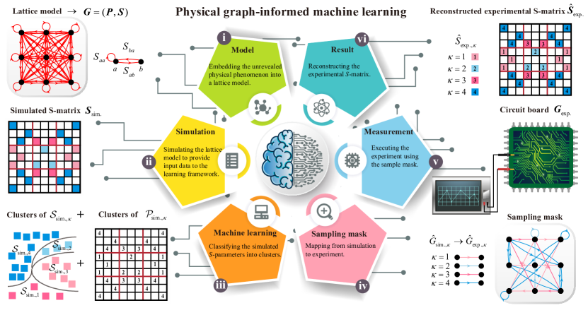
Figure 1: PGIML framework. (i) A lattice model embedding the unrevealed physical phenomenon is generated. The directional red circles and lines correspond to $S_{aa}$ and $S_{ab}$, respectively. (ii) The simulated $S$-matrix ${\textit{{S}}}_{\rm{sim.}}$ of the $L\times L$ lattice model is constructed and $N\times N$ ($N=L^{2}$) elements of a learning set $\mathcal{G}_{\rm{sim.}}=(\mathcal{P}_{\rm{sim.}},\mathcal{S}_{\rm{sim.}})$ are accumulated. (iii) $\mathcal{P}_{\rm{sim.}}$ and $\mathcal{S}_{\rm{sim.}}$ are classified into clusters $\mathcal{P}_{\rm{sim.},\kappa}$ and $\mathcal{S}_{\rm{sim.},\kappa}$ using the $K$-means method. (iv) A sampling mask corresponding to the graph-to-graph mapping $\hat{G}_{\rm{sim.},\kappa}\to\hat{G}_{\rm{exp.},\kappa}$ is generated. (v) The representative experimental $S$-parameters $\hat{S}_{\rm{exp.},\kappa}$ are measured in the circuit. (vi) The reconstructed experimental $S$-matrix $\hat{\textit{{S}}}_{\rm{exp.}}$ is retrieved.

We depict the PGIML framework in Fig. 1: (i) A lattice model that embeds the unrevealed physical phenomenon is generated and converted into a matrix of graphs G. (ii) The simulated $S$-matrix ${\textit{{S}}}_{\rm{{sim.}}}$ of the circuit is constructed and a learning set ${\cal G}_{\rm{sim.}}=({\cal P}_{\rm{sim.}},{\cal S}_{\rm{sim.}})$ is accumulated. (iii) The set of simulated positions ${{\cal P}_{{\rm{sim.}}}}$ and the set of simulated $S$-parameters ${{{\cal S}_{{\rm{sim.}}}}}$ are classified into clusters ${{{\cal P}_{{\rm{sim.},\kappa}}}}$ and ${{{\cal S}_{{\rm{sim.},\kappa}}}}$ using the $K$-means method (see Supplementary Material Sec. S3). (iv) The graph-to-graph mapping ${{\hat{G}}_{{\rm{sim}}.,\kappa}}\to{{\hat{G}}_{\exp.,\kappa}}$ is translated into a sampling mask that mirrors the clustering information. (v) The representative experimental $S$-parameters ${\hat{S}}_{{\rm{exp}}.,\kappa}$ are measured in the circuit. (vi) The $S$-matrix is encoded with the measured features $\bigcup\limits_{\kappa=1}^{K}{\{{{\hat{S}}_{\exp.,\kappa}}\}}$ and the reconstructed experimental $S$-matrix ${\hat{{\textit{{S}}}}_{\rm{exp.}}}$ is retrieved. The experimental $S$-matrix ${\textit{{S}}}_{\rm{{exp.}}}$ is then given by

$$\begin{array}[]{l}{{\textit{{S}}}_{\rm{exp.}}}\sim{\hat{{\textit{{S}}}}_{\rm{exp.}}}=\sum\limits_{\kappa=1}^{K}{{\hat{S}}_{{\rm{exp.}},\kappa}}\sum\limits_{(a,b)\in{{\mathcal{P}}_{{\rm{sim.}},\kappa}}}{{{\textit{{E}}}_{ab}}},\end{array}$$ (1)

where ${\textit{{E}}}_{ab}$ is a single-entry matrix (element $ab$ is one and the other elements are zero) [67]. Compared to conventional measurements of $N^{2}$ elements, the PGIML method is $N^{2}/K$ times faster, as it filters out redundancies, especially efficient for circuits that are too complex for a human to process.

Second-order non-Hermitian skin effect

We are now set up to explore the second-order NHSE, which gives rise to new types of boundary modes as a result of higher-order non-Hermitian topology. In a $L\times L$ lattice model, a first-order TI has ${\cal{O}}(L)$ edge modes with a gapless edge spectrum in the $x$ and $y$-directions. A second-order TI has ${\cal{O}}(1)$ corner modes with a gapped edge spectrum in the $x$ and $y$-directions. The first-order NHSE features extensive ${\cal{O}}(L^{2})$ edge skin modes with a gapless complex-valued edge spectrum in the $x$ and $y$-directions. Distinct from the Hermitian limit and the first-order NHSE, the second-order NHSE features ${\cal{O}}(L)$ corner skin modes with a gapless complex-valued edge spectrum in one direction and no edge spectrum in the other direction (see Supplementary Material Sec. S2). Schematic diagrams of these four situations are shown in Fig. 2. The explicit violation of the conventional bulk-boundary correspondence clearly demonstrates that modification of the topological band theory is inevitable in higher-dimensional non-Hermitian systems.

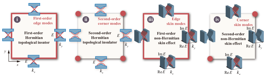
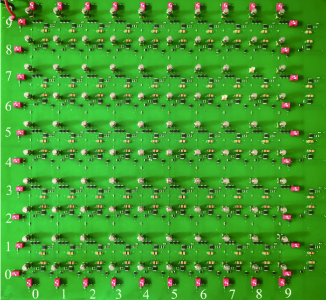
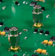
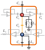
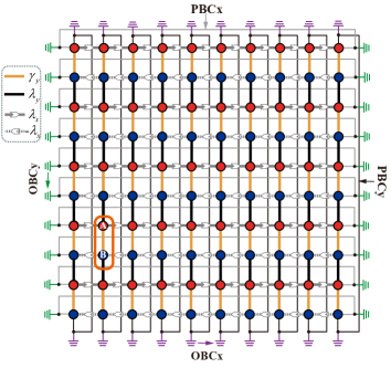
Figure 2: Second-order NHSE in a non-Hermitian circuit. $\bf{a}$, Schematic diagrams of topological band theory for the first-order TI, second-order TI, first-order NHSE, and second-order NHSE. $\bf{b}$, Photograph of the circuit. $\bf{c}$, Photograph of the unit cell. $\bf{d}$, Scheme of the unit cell. $\bf{e}$, Tight-binding analog of the circuit. The circuit components are represented by the intracell coupling $\gamma_{y}$ $(C_{2})$, intercell coupling $\lambda_{y}$ $(C_{1})$, and intercell non-reciprocal couplings $\lambda_{x}$ ($C_{1}$ connected to a voltage follower) and $-\lambda_{x}$ ($L_{1}$ reversely connected to a voltage follower). The grounding components are $L_{1}L_{2}/(L_{1}+2L_{2})$ and $L_{2}$ for sublattices A and B, respectively. PBC$x$ (grey), PBC$y$ (black), OBC$x$ (green), and OBC$y$ (purple) are controlled by the switches connecting the boundaries (see Supplementary Material Sec. S4).

To realize the second-order NHSE experimentally, we design a topoelectrical circuit that represents a 2D non-Hermitian two-band model. The $10\times 10$ circuitry lattice is shown in Fig. 2 and the unit cell is shown in Fig. 2 as photograph and in Fig. 2 as scheme. The tight-binding analog of the circuit is shown in Fig. 2 with intracell couplings $\gamma_{y}$, intercell couplings $\lambda_{y}$ in the $y$-direction, and intercell non-reciprocal couplings $\pm\lambda_{x}$ in the $x$-direction.

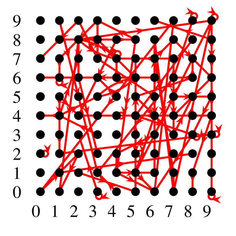
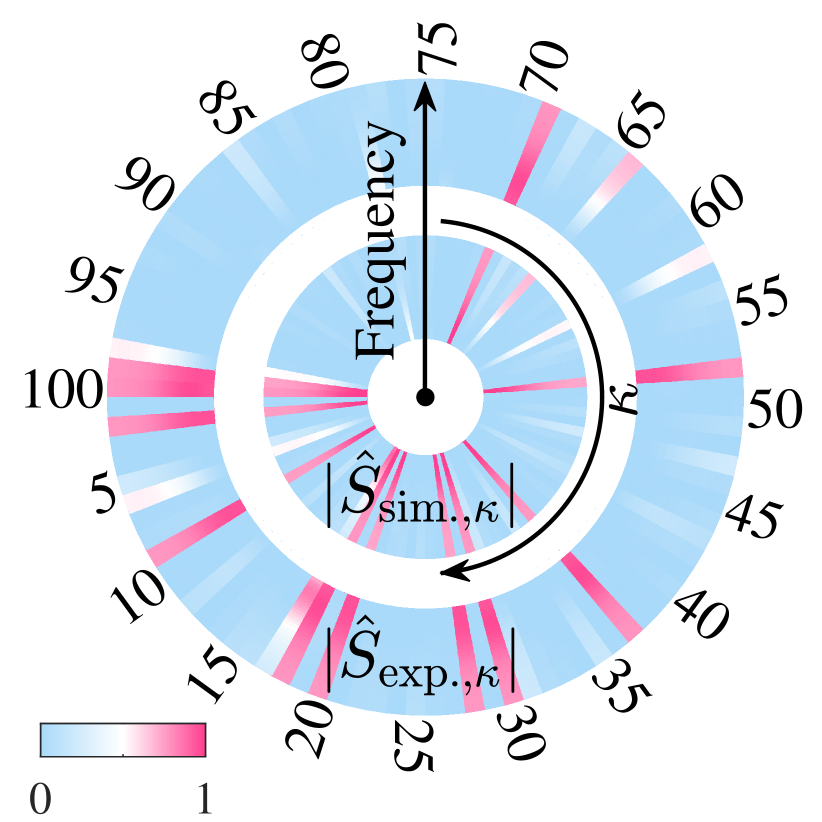
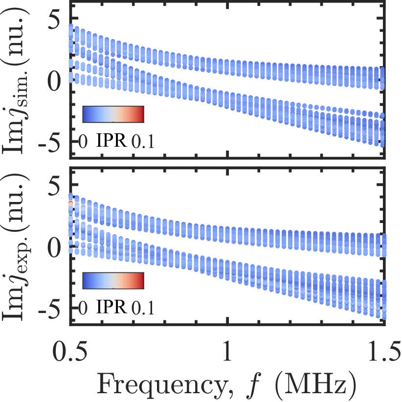
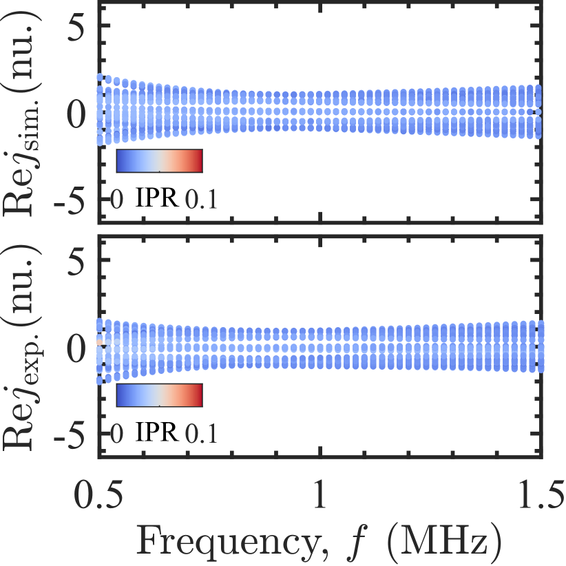
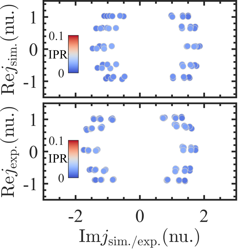
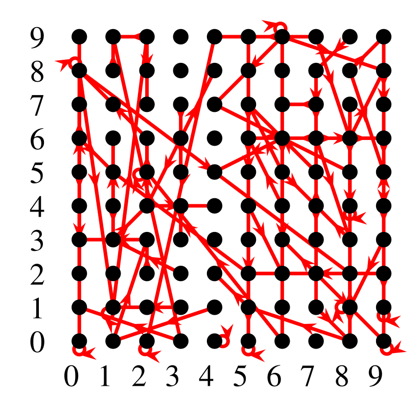
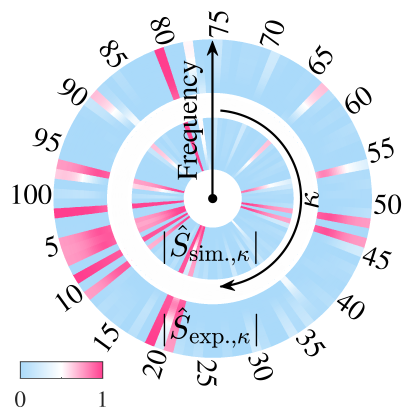
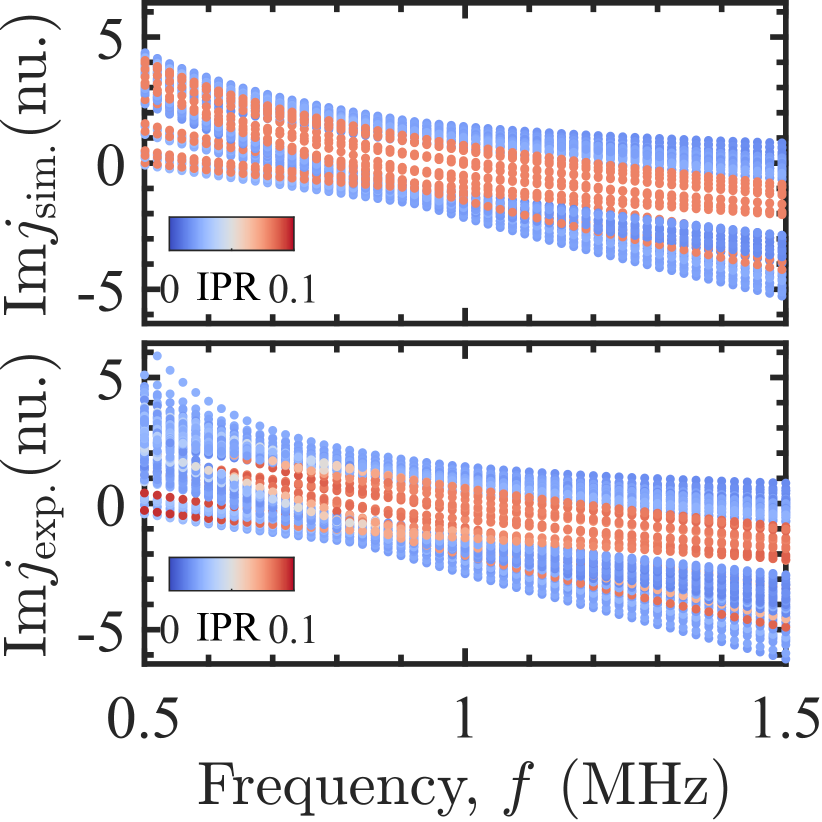
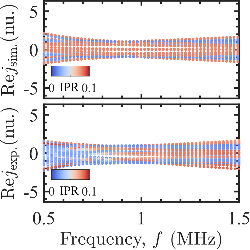
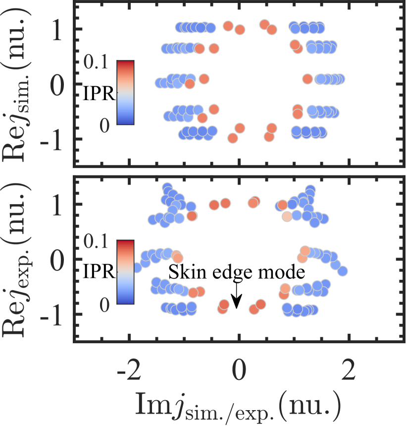
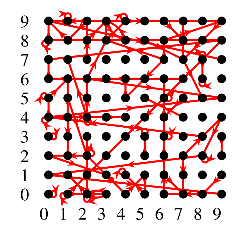
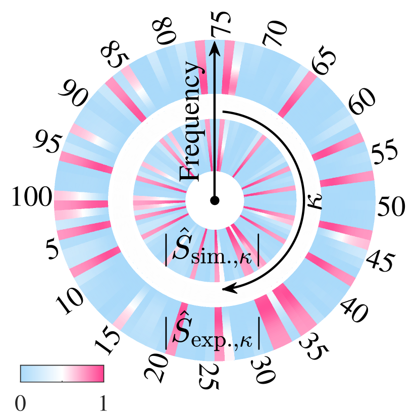
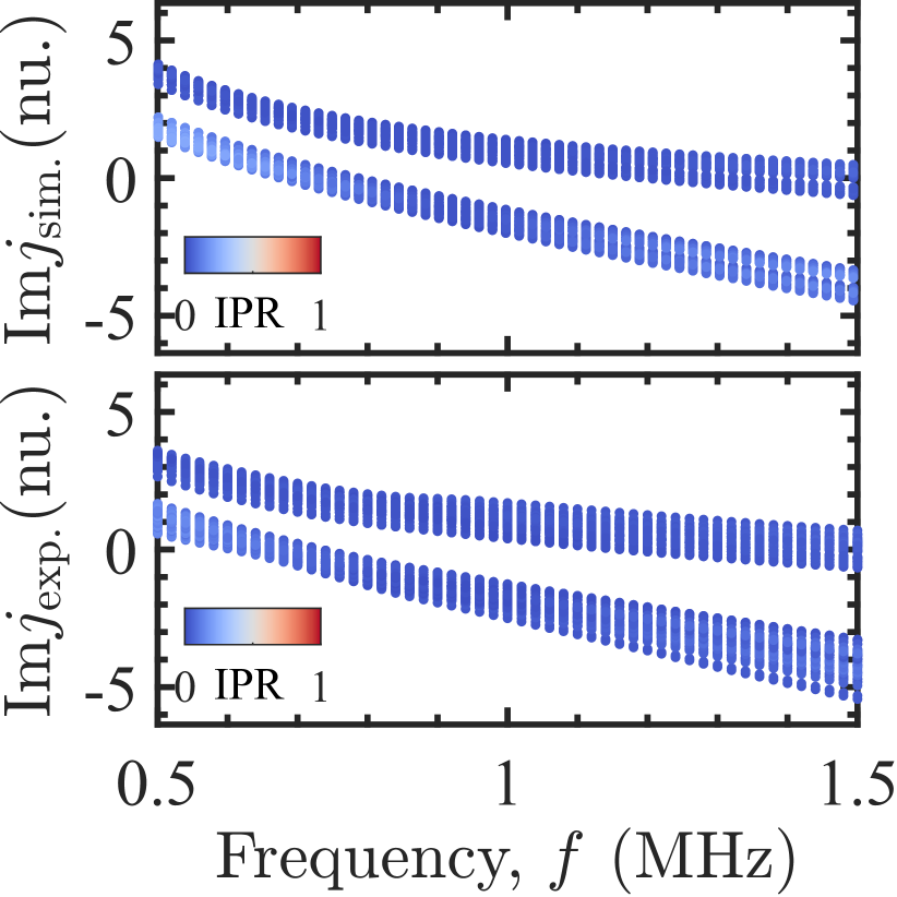
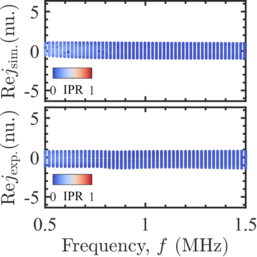
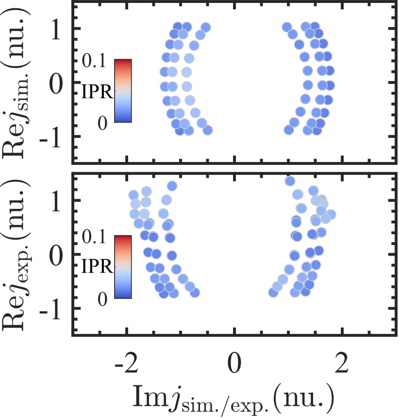
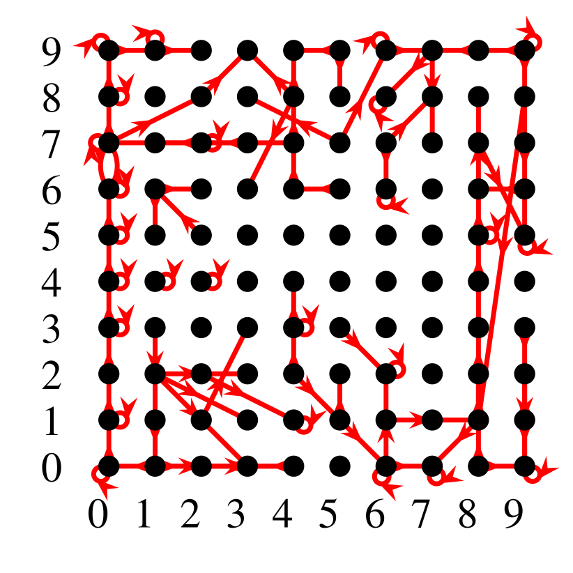
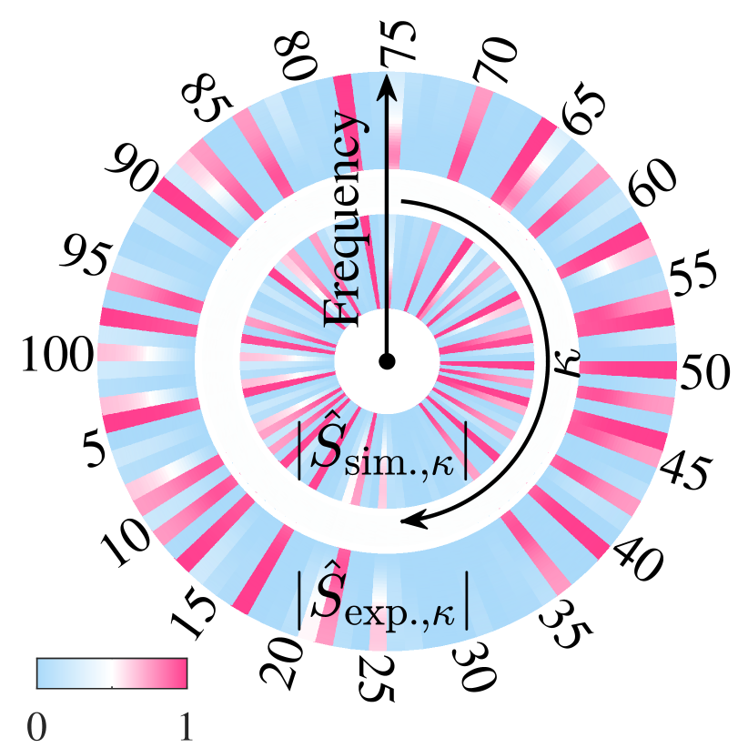
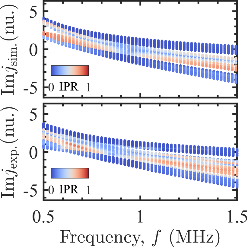
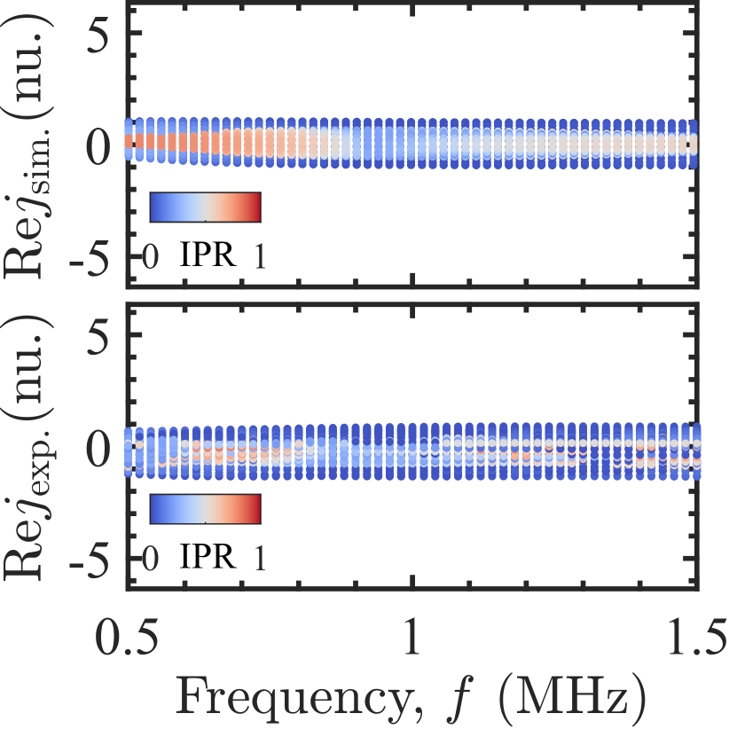
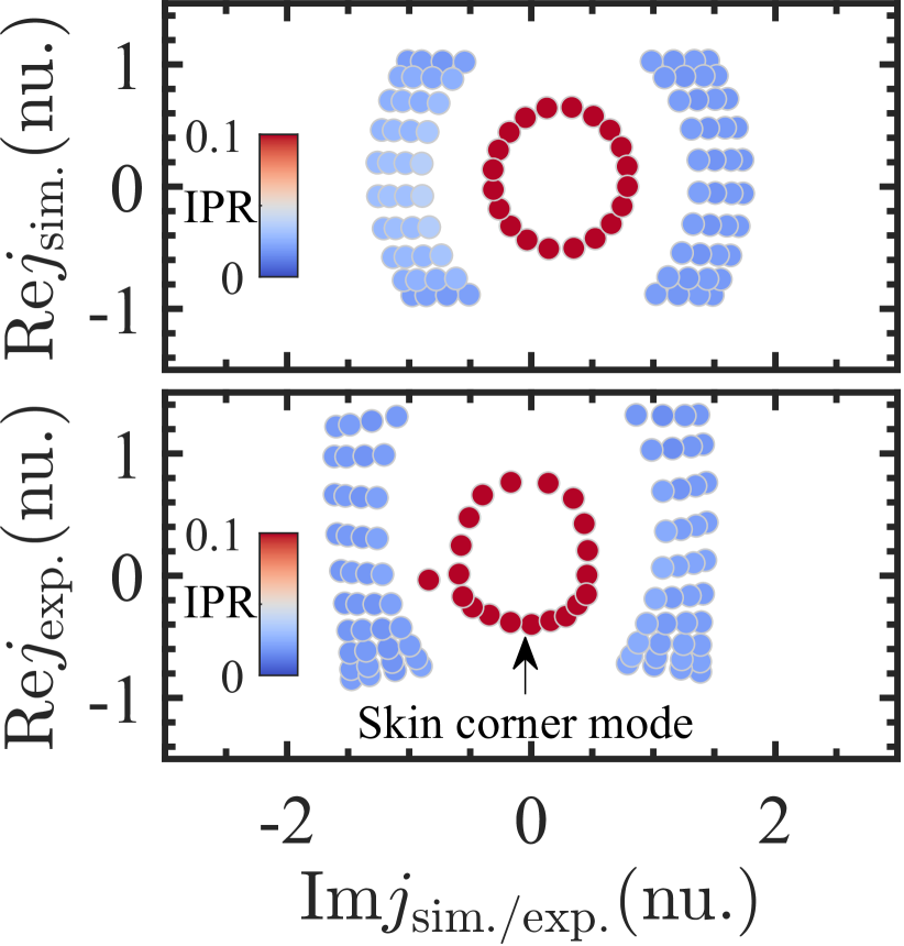
Figure 3: Comparison of experimental and simulated results for different boundary conditions. $\bf{a,f,k,p}$, Representative $S$-parameters are measured between ports connected by red directional circles and lines for $\kappa=1,2,\cdots,100$. $\bf{b,g,l,q}$, Frequency response of $|{{\hat{S}}_{\rm{sim.},\kappa}|}$ (inner circle) and $|{{\hat{S}}_{\rm{exp.},\kappa}|}$ (outer circle) for each $\kappa$, showing excellent agreement. $\bf{c,d,h,i,m,n,r,s}$, Imaginary and real parts of the admittance spectra $j_{\rm{sim.}}$ (top panel) and $j_{\rm{exp.}}$ (bottom panel) as functions of the driving frequency $f$, weighted by the IPR. $\bf{e,j,o,t,}$ Complex admittance spectra for the resonance frequency $f_{0}\sim 0.876\mathop{\rm{MHz}}$.

According to Kirchhoff’s laws, any circuit can be described by the block diagonal admittance matrix (circuit Laplacian) ${\textit{{J}}}(\omega)={{\rm{i}}\omega{\textit{{C}}}+\frac{1}{{{\rm{i}}\omega}}{{\textit{{W}}}}}$, where C and W are the Laplacian matrices of the capacitance and inverse inductance, respectively. For a given input current of frequency $\omega=2\pi f$, we obtain the non-reciprocal two-band admittance matrix (see Supplementary Material Sec. S1)

$${\textit{{J}}}({\textit{{k}}},\omega)={\rm{i}}\omega\left[{\begin{array}[]{*{20}{c}}{\frac{{{L_{1}}{L_{2}}}}{{\left({{L_{1}}+2{L_{2}}}\right){\omega^{2}}}}-2{C_{1}}-{C_{2}}+{C_{1}}{e^{-{\rm{i}}{k_{x}}}}}&{{C_{2}}+{C_{1}}{e^{-{\rm{i}}{k_{y}}}}}\\ {{C_{2}}+{C_{1}}{e^{{\rm{i}}{k_{y}}}}}&{\frac{{{L_{1}}{L_{2}}}}{{\left({{L_{1}}+{L_{2}}}\right){\omega^{2}}}}-{C_{1}}-{C_{2}}-\frac{{{L_{1}}}}{{{\omega^{2}}}}{e^{{\rm{i}}{k_{x}}}}}\end{array}}\right],$$ (2)

where two pairs of capacitors and inductors, $(C_{1},L_{1})$ and $(C_{2},L_{2})$, with the same resonance frequency ${\omega_{0}}={1\mathord{\left/{\vphantom{1{\sqrt{{L_{1}}{C_{1}}}}}}\right.\kern-1.2pt}{\sqrt{{L_{1}}{C_{1}}}}}={1\mathord{\left/{\vphantom{1{\sqrt{{L_{2}}{C_{2}}}}}}\right.\kern-1.2pt}{\sqrt{{L_{2}}{C_{2}}}}}$ are used to couple the nodes. This implies

$${\textit{{J}}}({{\textit{{k}}}},{\omega_{0}})={\rm{i}}\sqrt{{{{C_{1}}}\mathord{\left/{\vphantom{{{C_{1}}}{{L_{1}}}}}\right.\kern-1.2pt}{{L_{1}}}}}\left[-{\rm{i}}{\lambda_{x}}\sin{k_{x}}{\sigma_{0}}+{\lambda_{x}}\cos{k_{x}}{\sigma_{z}}+{\lambda_{y}}\sin{k_{y}}{\sigma_{y}}+\left({{\gamma_{y}}+{\lambda_{y}}\cos{k_{y}}}\right){\sigma_{x}}\right].$$ (3)

For ${C_{1}}=1000\mathop{\rm{pH}}$, ${C_{2}}=330\mathop{\rm{pH}}$, ${L_{1}}=33\mathop{\mu}{\rm{F}}$, and ${L_{2}}=100\mathop{\mu}{\rm{F}}$, we arrive at $\lambda_{x}=1$, $\lambda_{y}=1$, and $\gamma_{y}=0.33$. The eigenvalues of ${\textit{{J}}}({{\textit{{k}}}},{\omega_{0}})$ are given by

$$j({\textit{{k}}},{\omega_{0}})={\rm{i}}\sqrt{{C_{1}}/{L_{1}}}(\pm\sqrt{{\lambda_{x}}^{2}{{\cos}^{2}}{k_{x}}+2{\lambda_{y}}{\gamma_{y}}\cos{k_{y}}+{\lambda_{y}}^{2}+\gamma_{y}^{2}}{\rm{-i}}{\lambda_{x}}\sin{k_{x}}).$$ (4)

As the boundary connections can be customized, we can observe phase transitions through differences in the spectral flow, enabling the study of the topological modes at any choice of boundary conditions. The admittance eigenvalues and eigenstates are accessible by an $S$-parameter measurement using the PGIML framework. We address the circuit for PBC$x$-PBC$y$ in Figs. 3-e, for PBC$x$-OBC$y$ in Figs. 3-j, for OBC$x$-PBC$y$ in Figs. 3-o, and for PBC$x$-PBC$y$ in Figs. 3-t. Figures 3,f,k,p show the ports selected for measuring the representative $S$-parameters (see Supplementary Material Sec. S4). According to Figs. 3,g,l,q, the frequency response of $|{{\hat{S}}_{\rm{exp.},\kappa}|}$ (outer circle) agrees well with that of $|{{\hat{S}}_{\rm{sim.},\kappa}|}$ (inner circle). Figures 3,h,m,r and 3,i,n,s show the imaginary and real parts, respectively, of the simulated (top panel) and experimental (bottom panel) admittance spectra as functions of the driving frequency $f$, weighted by the inverse participation ratio $\rm{IPR}=\sum\limits_{n}{{{|{{\Psi_{n}}}|}^{4}}}/{({\sum\limits_{n}{{{|{{\Psi_{n}}}|}^{2}}}})^{2}}$, where $\Psi_{n}$ is the $n$-th eigenmode. A larger IPR corresponds to a more localized mode. For simplicity, the results are given in normalized units (nu.) as multiplies of $\sqrt{{L_{1}}/{C_{1}}}\mathop{\Omega}^{-1}$. Figures. 3,j,o,t show the simulated and experimental admittance spectra in the complex plane at the resonance frequency $f_{0}=\left(2\pi\sqrt{L_{1}C_{1}}\right)^{-1}\sim 0.876\mathop{\mathrm{MHz}}$. The system has trivial topology without NHSE for PBC$x$-PBC$y$ and OBC$x$-PBC$y$, and non-trivial topology with NHSE for PBC$x$-OBC$y$ and OBC$x$-OBC$y$. In particular, figure 3 shows skin edge modes for PBC$x$-OBC$y$. We observe in Fig. 4 a localized mode distribution at the left/right boundary, in contrast to the delocalized bulk modes. Remarkably, the skin corner modes in Fig. 3 form a circle in the complex-energy plane for OBC$x$-OBC$y$, analytically given by $j_{\rm{sim.}}=0.33\sqrt{{C_{1}}/{L_{1}}}{e^{{\rm{i}}\theta}},\theta\in\left[{0,2\pi}\right]$ (see Supplementary Material Sec. S2). They are localized at the corners while the bulk modes are delocalized, as can be seen in Fig. 4. A non-Bloch 2D winding number $v_{2D}=1$ characterizes the higher-order NHSE (Methods). For all the $L^{2}$ eigenmodes, the number of corner skin modes is $2L$ while the number of delocalized bulk modes is $L^{2}-2L$.

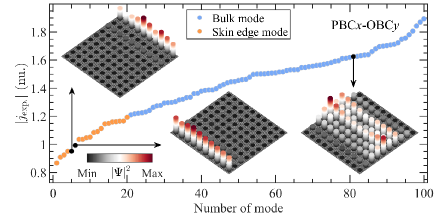
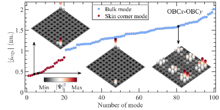
Figure 4: Admittance spectra and mode distributions. $\bf{a}$, Absolute values of $j_{\rm{exp.}}$ for PBC$x$-OBC$y$. $\bf{b}$, Absolute values of $j_{\rm{exp.}}$ for OBC$x$-OBC$y$. The insets show the bulk and skin edge/corner modes.

Conclusion

In times of digital research and measurement, many scientific disciplines produce large amounts of data that by far surpass conventional computational abilities for processing and analyzing. Hence, we develop the PGIML method by integrating physical principles, graph visualization of features, and ML to enforce the identification of an unrevealed physical phenomenon. At the example of a topoelectrical circuit, we embed the physical principles of the second-order NHSE into the circuit, observe the skin corner modes, demonstrate the violation of the conventional bulk-boundary correspondence, and reveal an intriguing interplay between higher-order topology and non-Hermiticity. Our results suggest that the PGIML method provides a paradigm shift in processing and analyzing data, opening new avenues to understanding complex systems in higher dimensions.

Methods

Topological invariant

According to point-gap topology [68, 31, 41], we derive a topological characterization of the NHSE. A non-Hermitian Hamiltonian $H$ has a point gap at a reference point $E\in{\mathbb{C}}$ if and only if its complex spectrum does not cross $E$, i.e., $\det(H-E)\neq 0$. The topological invariant is given by the winding number

$$w(E)=\int_{0}^{2\pi}{\frac{{dk}}{{2\pi{\rm{i}}}}\frac{d}{{dk}}\log\det[H(k)-E]},$$ (5)

where $H(k)$ is the non-Hermitian Bloch Hamiltonian. The second-order NHSE occurs when $w(E)\neq 0$. The non-Hermitian topology of $H(k)$ can also be understood in terms of the extended Hermitian Hamiltonian

$$\tilde{H}(k,E)=\left({\begin{array}[]{*{20}{c}}0&{H(k)-E}\\ {{H^{\dagger}}(k)-{E^{*}}}&0\end{array}}\right),$$ (6)

which is topologically nontrivial with a finite energy gap if and only if $H(k)$ is topologically nontrivial with a point gap at $E$.

To clarify the topological property of the second-order NHSE [69, 70, 71], we define the extended Hermitian admittance Hamiltonian

$$\tilde{J}({{\textit{{k}}}},{\omega_{0}})=\left({\begin{array}[]{*{20}{c}}0&{J({{\textit{{k}}}},{\omega_{0}})-j}\\ {{J^{\dagger}}({{\textit{{k}}}},{\omega_{0}})-{j^{*}}}&0\end{array}}\right),$$ (7)

and perform the unitary transformation $\tilde{\cal{J}}({{\textit{{k}}}},{\omega_{0}})=\textit{{U}}\tilde{J}({{\textit{{k}}}},{\omega_{0}}){\textit{{U}}^{\dagger}}$ using

$$\textit{{U}}=\left({\begin{array}[]{*{20}{c}}0&0&0&{-1}\\ 1&0&0&0\\ 0&{-1}&0&0\\ 0&0&1&0\end{array}}\right).$$ (8)

We obtain

$$\tilde{\cal{J}}({{\textit{{k}}}},{\omega_{0}})={\tilde{\cal{J}}_{x}}({k_{x}},{\omega_{0}})\otimes{\tau_{z}}+{\sigma_{0}}\otimes{\tilde{\cal{J}}_{y}}({k_{y}},{\omega_{0}}),$$ (9)

with

$$\begin{array}[]{*{20}{c}}{{\tilde{\cal{J}}_{x}}({k_{x}},{\omega_{0}})=-{\rm{i}}\sqrt{{{{C_{1}}}\mathord{\left/{\vphantom{{{C_{1}}}{{L_{1}}}}}\right.\kern-1.2pt}{{L_{1}}}}}\left[{{\lambda_{x}}\cos{k_{x}}{\sigma_{x}}+({\lambda_{x}}\sin{k_{x}}-E){\sigma_{y}}}\right]},\\ {{\tilde{\cal{J}}_{y}}({k_{y}},{\omega_{0}})=-{\rm{i}}\sqrt{{{{C_{1}}}\mathord{\left/{\vphantom{{{C_{1}}}{{L_{1}}}}}\right.\kern-1.2pt}{{L_{1}}}}}\left[{({\lambda_{y}}\cos{k_{y}}+{\gamma_{y}}){\tau_{x}}-{\lambda_{y}}\sin{k_{y}}{\tau_{y}}}\right]}.\end{array}$$ (10)

Both ${\tilde{\cal{J}}_{x}}({k_{x}},{\omega_{0}})$ and ${\tilde{\cal{J}}_{y}}({k_{x}},{\omega_{0}})$ have chiral symmetry corresponding to $\sigma_{z}$ and $\tau_{z}$, respectively. Since chirality and inversion symmetry here commute, the non-Hermitian topology of $\tilde{\cal{J}}({{\textit{{k}}}},{\omega_{0}})$ is characterized by the chiral symmetry ${\cal{C}}={\sigma_{z}}\otimes{\tau_{z}}$. Thus, the second-order NHSE is characterized by the $\mathbb{Z}$ topological invariant [71, 40]

$${v_{2D}}={w_{x}}{w_{y}},$$ (11)

with the winding numbers

$${w_{\alpha}}(j)=\int_{0}^{2\pi}{\frac{{d{k_{\alpha}}}}{{2\pi{\rm{i}}}}\frac{d}{{d{k_{\alpha}}}}\log\det[\tilde{\cal{J}}_{\alpha}({k_{\alpha}},{\omega_{0}})-j]},$$ (12)

where $\alpha=x,y$. Thus, $w_{x}=1$ as $E\in(-\lambda_{x},\lambda_{x})$ and $w_{y}=1$ as $\lambda_{y}/{\gamma_{y}}>1$. Hence, we obtain a nonzero topological invariant ${v_{2D}}=1$ if and only if $E\in(-\lambda_{x},\lambda_{x})$ and $\lambda_{y}/{\gamma_{y}}>1$. ${v_{2D}}$ changes when the edge and bulk modes close the gap, establishing the second-order non-Hermitian topology.

Experiment

Nonreciprocal couplings are realized by voltage feedback operational amplifiers (Texas Instruments, LM6171), which block the input current while maintaining the output current. To ensure small linewidths of the circuit Laplacian spectra, we use high-Q inductors (Murata, Q-factor $>40$with $5{\%}$ component variation). Additional elements are added to the circuit to increase the stability of the voltage feedback operational amplifiers, including a $5\mathop{\Omega}$ resistor connected in series at the output and a $2000\mathop{\Omega}$ resistor in shunt with a $100\mathop{\rm{pF}}$ capacitor connecting across the inverting input and output of the voltage feedback operational amplifier. The circuit Laplacian spectra are obtained by measuring the $S$-parameters of the circuit at $10\mathop{\rm{kHz}}$ frequency resolution. We employ a vector network analyzer (Tektronix TTr500) and transform the $S$-matrix into the circuit Laplacian using the impedance matrix, i.e., the inverse of the circuit Laplacian ${\textit{{J}}}^{-1}={Z_{0}}({\textit{{S}}}+{\mathbb{I}}){({\mathbb{I}}-{\textit{{S}}})^{-1}}$, where $\mathbb{I}$ is the identity matrix and $Z_{0}$ is the characteristic impedance. In an $S$-parameter measurement between two ports, the other ports are connected with $50\mathop{\Omega}$ load terminators to ensure zero reflection. Note that the impedance matrix obtained by our method is equivalent to that obtained by current probes [72, 73], while the measurement is simplified dramatically and the experimental stability is improved.

Author contributions

C.S. and S.L. conceived the idea. C.S. performed the theoretical analyses. C.S., S.L., and R.S. designed the circuits and performed the experiments. C.S. and P.H. developed the machine learning method. C.H.L. and R.T. evaluated the experimental and numerical results. A.M., S.Z., T.J.C., and U.S. guided the research. All the authors contributed to the discussions of the results and the preparation of the manuscript.

Data availability statement

The datasets generated and analyzed in the current study are available from the corresponding author on reasonable request.

Competing interests

The authors declare no competing interests.

References

- Hasan and Kane [2010] M. Z. Hasan and C. L. Kane, Colloquium: Topological insulators, Rev. Mod. Phys. 82, 3045 (2010).
- Qi and Zhang [2011] X.-L. Qi and S.-C. Zhang, Topological insulators and superconductors, Rev. Mod. Phys. 83, 1057 (2011).
- Bansil et al. [2016] A. Bansil, H. Lin, and T. Das, Colloquium: Topological band theory, Rev. Mod. Phys. 88, 021004 (2016).
- Sessi et al. [2016] P. Sessi, D. D. Sante, A. Szczerbakow, F. Glott, S. Wilfert, H. Schmidt, T. Bathon, P. Dziawa, M. Greiter, T. Neupert, G. Sangiovanni, T. Story, R. Thomale, and M. Bode, Robust spin-polarized midgap states at step edges of topological crystalline insulators, Science 354, 1269 (2016).
- Benalcazar et al. [2017a] W. A. Benalcazar, B. A. Bernevig, and T. L. Hughes, Quantized electric multipole insulators, Science 357, 61 (2017a).
- Benalcazar et al. [2017b] W. A. Benalcazar, B. A. Bernevig, and T. L. Hughes, Electric multipole moments, topological multipole moment pumping, and chiral hinge states in crystalline insulators, Phys. Rev. B 96, 245115 (2017b).
- Peng et al. [2017] Y. Peng, Y. Bao, and F. von Oppen, Boundary Green functions of topological insulators and superconductors, Phys. Rev. B 95, 235143 (2017).
- Song et al. [2017] Z. Song, Z. Fang, and C. Fang, -dimensional edge states of rotation symmetry protected topological states, Phys. Rev. Lett. 119, 246402 (2017).
- Langbehn et al. [2017] J. Langbehn, Y. Peng, L. Trifunovic, F. von Oppen, and P. W. Brouwer, Reflection-symmetric second-order topological insulators and superconductors, Phys. Rev. Lett. 119, 246401 (2017).
- Schindler et al. [2018] F. Schindler, A. M. Cook, M. G. Vergniory, Z. Wang, S. S. P. Parkin, B. A. Bernevig, and T. Neupert, Higher-order topological insulators, Sci. Adv. 4, eaat0346 (2018).
- Ezawa [2018] M. Ezawa, Magnetic second-order topological insulators and semimetals, Phys. Rev. B 97, 155305 (2018).
- Sheng et al. [2019] X.-L. Sheng, C. Chen, H. Liu, Z. Chen, Z.-M. Yu, Y. X. Zhao, and S. A. Yang, Two-dimensional second-order topological insulator in graphdiyne, Phys. Rev. Lett. 123, 256402 (2019).
- Park et al. [2019] M. J. Park, Y. Kim, G. Y. Cho, and S. Lee, Higher-order topological insulator in twisted bilayer Graphene, Phys. Rev. Lett. 123, 216803 (2019).
- Chen et al. [2020] R. Chen, C.-Z. Chen, J.-H. Gao, B. Zhou, and D.-H. Xu, Higher-order topological insulators in quasicrystals, Phys. Rev. Lett. 124, 036803 (2020).
- Huang and Liu [2020] B. Huang and W. V. Liu, Floquet higher-order topological insulators with anomalous dynamical polarization, Phys. Rev. Lett. 124, 216601 (2020).
- Ren et al. [2020] Y. Ren, Z. Qiao, and Q. Niu, Engineering corner states from two-dimensional topological insulators, Phys. Rev. Lett. 124, 166804 (2020).
- Rüter et al. [2010] C. E. Rüter, K. G. Makris, R. El-Ganainy, D. N. Christodoulides, M. Segev, and D. Kip, Observation of parity-time symmetry in optics, Nat. Phys. 6, 192 (2010).
- Regensburger et al. [2012] A. Regensburger, C. Bersch, M.-A. Miri, G. Onishchukov, D. N. Christodoulides, and U. Peschel, Parity-time synthetic photonic lattices, Nature 488, 167 (2012).
- Peng et al. [2014] B. Peng, Ş. K. Özdemir, F. Lei, F. Monifi, M. Gianfreda, G. L. Long, S. Fan, F. Nori, C. M. Bender, and L. Yang, Parity-time-symmetric whispering-gallery microcavities, Nat. Phys. 10, 394 (2014).
- Zhang et al. [2018] J. Zhang, B. Peng, Ş. K. Özdemir, K. Pichler, D. O. Krimer, G. Zhao, F. Nori, Y.-X. Liu, S. Rotter, and L. Yang, A phonon laser operating at an exceptional point, Nat. Photon. 12, 479 (2018).
- Zhou et al. [2018] H. Zhou, C. Peng, Y. Yoon, C. W. Hsu, K. A. Nelson, L. Fu, J. D. Joannopoulos, M. Soljačić, and B. Zhen, Observation of bulk Fermi arc and polarization half charge from paired exceptional points, Science 359, 1009 (2018).
- Hodaei et al. [2017] H. Hodaei, A. U. Hassan, S. Wittek, H. Garcia-Gracia, R. El-Ganainy, D. N. Christodoulides, and M. Khajavikhan, Enhanced sensitivity at higher-order exceptional points, Nature 548, 187 (2017).
- Chen et al. [2017] W. Chen, Ş. K. Özdemir, G. Zhao, J. Wiersig, and L. Yang, Exceptional points enhance sensing in an optical microcavity, Nature 548, 192 (2017).
- Hodaei et al. [2014] H. Hodaei, M.-A. Miri, M. Heinrich, D. N. Christodoulides, and M. Khajavikhan, Parity-time-symmetric microring lasers, Science 346, 975 (2014).
- Brandstetter et al. [2014] M. Brandstetter, M. Liertzer, C. Deutsch, P. Klang, J. Schöberl, H. E. Türeci, G. Strasser, K. Unterrainer, and S. Rotter, Reversing the pump dependence of a laser at an exceptional point, Nat. Commun. 5, 4034 (2014).
- Weimann et al. [2017] S. Weimann, M. Kremer, Y. Plotnik, Y. Lumer, S. Nolte, K. G. Makris, M. Segev, M. C. Rechtsman, and A. Szameit, Topologically protected bound states in photonic parity-time-symmetric crystals, Nat. Mater. 16, 433 (2017).
- Bahari et al. [2017] B. Bahari, A. Ndao, F. Vallini, A. E. Amili, Y. Fainman, and B. Kanté, Nonreciprocal lasing in topological cavities of arbitrary geometries, Science 358, 636 (2017).
- Bandres et al. [2018] M. A. Bandres, S. Wittek, G. Harari, M. Parto, J. Ren, M. Segev, D. N. Christodoulides, and M. Khajavikhan, Topological insulator laser: Experiments, Science 359, eaar4005 (2018).
- Harari et al. [2018] G. Harari, M. A. Bandres, Y. Lumer, M. C. Rechtsman, Y. D. Chong, M. Khajavikhan, D. N. Christodoulides, and M. Segev, Topological insulator laser: Theory, Science 359, eaar4003 (2018).
- Kunst et al. [2018] F. K. Kunst, E. Edvardsson, J. C. Budich, and E. J. Bergholtz, Biorthogonal bulk-boundary correspondence in non-Hermitian systems, Phys. Rev. Lett. 121, 026808 (2018).
- Kawabata et al. [2019] K. Kawabata, K. Shiozaki, M. Ueda, and M. Sato, Symmetry and topology in non-Hermitian physics, Phys. Rev. X 9, 041015 (2019).
- Yokomizo and Murakami [2019] K. Yokomizo and S. Murakami, Non-Bloch band theory of non-Hermitian systems, Phys. Rev. Lett. 123, 066404 (2019).
- Yao and Wang [2018] S. Yao and Z. Wang, Edge states and topological invariants of non-Hermitian systems, Phys. Rev. Lett. 121, 086803 (2018).
- Song et al. [2019] F. Song, S. Yao, and Z. Wang, Non-Hermitian skin effect and chiral damping in open quantum systems, Phys. Rev. Lett. 123, 170401 (2019).
- Luo and Zhang [2019] X.-W. Luo and C. Zhang, Higher-order topological corner states induced by gain and loss, Phys. Rev. Lett. 123, 073601 (2019).
- Lee et al. [2019] C. H. Lee, L. Li, and J. Gong, Hybrid higher-order skin-topological modes in nonreciprocal systems, Phys. Rev. Lett. 123, 016805 (2019).
- Zhang et al. [2020] K. Zhang, Z. Yang, and C. Fang, Correspondence between winding numbers and skin modes in non-Hermitian systems, Phys. Rev. Lett. 125, 126402 (2020).
- Yang et al. [2020] Z. Yang, K. Zhang, C. Fang, and J. Hu, Non-Hermitian bulk-boundary correspondence and auxiliary generalized Brillouin zone theory, Phys. Rev. Lett. 125, 226402 (2020).
- Kawabata et al. [2020] K. Kawabata, M. Sato, and K. Shiozaki, Higher-order non-Hermitian skin effect, Phys. Rev. B 102, 205118 (2020).
- Okugawa et al. [2020] R. Okugawa, R. Takahashi, and K. Yokomizo, Second-order topological non-Hermitian skin effects, Phys. Rev. B 102, 241202 (2020).
- Okuma et al. [2020] N. Okuma, K. Kawabata, K. Shiozaki, and M. Sato, Topological origin of non-Hermitian skin effects, Phys. Rev. Lett. 124, 086801 (2020).
- Li et al. [2020] L. Li, C. H. Lee, S. Mu, and J. Gong, Critical non-Hermitian skin effect, Nat. Commun. 11, 5491 (2020).
- Lee and Longhi [2020] C. H. Lee and S. Longhi, Ultrafast and anharmonic Rabi oscillations between non-Bloch bands, Commun. Phys. 3, 147 (2020).
- Fu et al. [2021] Y. Fu, J. Hu, and S. Wan, Non-Hermitian second-order skin and topological modes, Phys. Rev. B 103, 045420 (2021).
- Li et al. [2021] L. Li, S. Mu, C. H. Lee, and J. Gong, Quantized classical response from spectral winding topology, Nat. Commun. 12, 5294 (2021).
- Helbig et al. [2020] T. Helbig, T. Hofmann, S. Imhof, M. Abdelghany, T. Kiessling, L. W. Molenkamp, C. H. Lee, A. Szameit, M. Greiter, and R. Thomale, Generalized bulk-boundary correspondence in non-Hermitian topolectrical circuits, Nat. Phys. 16, 747 (2020).
- Hofmann et al. [2020] T. Hofmann, T. Helbig, F. Schindler, N. Salgo, M. Brzezińska, M. Greiter, T. Kiessling, D. Wolf, A. Vollhardt, A. Kabaši, C. H. Lee, A. Bilušić, R. Thomale, and T. Neupert, Reciprocal skin effect and its realization in a topolectrical circuit, Phys. Rev. Research 2, 023265 (2020).
- Liu et al. [2021] S. Liu, R. Shao, S. Ma, L. Zhang, O. You, H. Wu, Y. J. Xiang, T. J. Cui, and S. Zhang, Non-Hermitian skin effect in a non-Hermitian electrical circuit, Research 2021, 1 (2021).
- Zhang et al. [2021] X. Zhang, Y. Tian, J.-H. Jiang, M.-H. Lu, and Y.-F. Chen, Observation of higher-order non-Hermitian skin effect, Nat. Commun. 12, 5377 (2021).
- Palacios et al. [2021] L. S. Palacios, S. Tchoumakov, M. Guix, I. Pagonabarraga, S. Sánchez, and A. G. Grushin, Guided accumulation of active particles by topological design of a second-order skin effect, Nat. Commun. 12, 4691 (2021).
- Weidemann et al. [2020] S. Weidemann, M. Kremer, T. Helbig, T. Hofmann, A. Stegmaier, M. Greiter, R. Thomale, and A. Szameit, Topological funneling of light, Science 368, 311 (2020).
- Carleo et al. [2019] G. Carleo, I. Cirac, K. Cranmer, L. Daudet, M. Schuld, N. Tishby, L. Vogt-Maranto, and L. Zdeborová, Machine learning and the physical sciences, Rev. Mod. Phys. 91, 045002 (2019).
- Mehta et al. [2019] P. Mehta, M. Bukov, C.-H. Wang, A. G. Day, C. Richardson, C. K. Fisher, and D. J. Schwab, A high-bias, low-variance introduction to machine learning for physicists, Phys. Rep. 810, 1 (2019).
- Buchanan [2019] M. Buchanan, The power of machine learning, Nature 15, 1208 (2019).
- Karniadakis et al. [2021] G. E. Karniadakis, I. G. Kevrekidis, L. Lu, P. Perdikaris, S. Wang, and L. Yang, Physics-informed machine learning, Nat. Rev. Phys. 3, 422 (2021).
- Kritzinger et al. [2018] W. Kritzinger, M. Karner, G. Traar, J. Henjes, and W. Sihn, Digital twin in manufacturing: A categorical literature review and classification, IFAC-PapersOnLine 51, 1016 (2018).
- Tao and Qi [2019] F. Tao and Q. Qi, Make more digital twins, Nature 573, 490 (2019).
- Singh et al. [2021] M. Singh, E. Fuenmayor, E. P. Hinchy, Y. Qiao, N. Murray, and D. Devine, Digital twin: Origin to future, Appl. Syst. Innov. 4, 36 (2021).
- Gelernter [1991] D. H. Gelernter, Mirror worlds, or, The day software puts the universe in a shoebox: How it will happen and what it will mean (Oxford University Press, Oxford, 1991).
- Grieves [2005] M. W. Grieves, Product lifecycle management: The new paradigm for enterprises, Int. J. Prod. Dev. 2, 71 (2005).
- Pozar [2011] D. M. Pozar, Microwave engineering (John Wiley & Sons, Hoboken, 2011).
- West [2001] D. B. West, Introduction to graph theory (Prentice Hall, Hoboken, 2001).
- Likas et al. [2003] A. Likas, N. Vlassis, and J. J. Verbeek, The global K-means clustering algorithm, Pattern Recognit. 36, 451 (2003).
- Wu [2012] J. Wu, Advances in K-means clustering: A data mining thinking (Springer, 2012).
- Moore [1982] G. H. Moore, Zermelo’s axiom of choice: Its origins, development, and influence (Springer, Berlin, 1982).
- Miller [1979] G. L. Miller, Graph isomorphism, general remarks, J. Comput. Syst. Sci. 18, 128 (1979).
- Petersen and Pedersen [2008] K. B. Petersen and Pedersen, The matrix cookbook (Technical University of Denmark, Lyngby, 2008).
- Gong et al. [2018] Z. Gong, Y. Ashida, K. Kawabata, K. Takasan, S. Higashikawa, and M. Ueda, Topological phases of non-Hermitian systems, Phys. Rev. X 8, 031079 (2018).
- Hayashi [2018] S. Hayashi, Topological invariants and corner states for Hamiltonians on a three-dimensional lattice, Commun. Math. Phys. 364, 343 (2018).
- Hayashi [2019] S. Hayashi, Toeplitz operators on concave corners and topologically protected corner states, Lett. Math. Phys. 109, 2223 (2019).
- Okugawa et al. [2019] R. Okugawa, S. Hayashi, and T. Nakanishi, Second-order topological phases protected by chiral symmetry, Phys. Rev. B 100, 235302 (2019).
- Ningyuan et al. [2015] J. Ningyuan, C. Owens, A. Sommer, D. Schuster, and J. Simon, Time- and site-resolved dynamics in a topological circuit, Phys. Rev. X 5, 021031 (2015).
- Lee et al. [2020] C. H. Lee, A. Sutrisno, T. Hofmann, T. Helbig, Y. Liu, Y. S. Ang, L. K. Ang, X. Zhang, M. Greiter, and R. Thomale, Imaging nodal knots in momentum space through topolectrical circuits, Nat. Commun. 11, 4385 (2020).