Deep learning study on the Dirac eigenvalue spectrum of staggered quarks

Abstract

We study the chirality of staggered quarks on the Dirac eigenvalue spectrum using deep learning (DL) techniques. The Kluberg-Stern method to construct staggered bilinear operators conserves continuum property such as recursion relations, uniqueness of chirality, and Ward identities, which leads to a unique and characteristic pattern (we call it “leakage pattern (LP)”) in the matrix elements of the chirality operator sandwiched between two quark eigenstates of staggered Dirac operator. DL analysis gives $99.4(2)\%$ accuracy on normal gauge configurations and $0.998$ AUC (Area Under ROC Curve) for classifying non-zero mode octets in the Dirac eigenvalue spectrum. It confirms that the leakage pattern is universal on normal gauge configurations. The multi-layer perceptron (MLP) method turns out to be the best DL model for our study on the LP.

1 Introduction

Here, we present technical details on how to do a deep learning analysis on low non-zero modes for staggered Dirac operators. This work is a follow-up paper on our previous papers: Ref. [1, 2, 3, 4].

2 Staggered Dirac eigenstate

Here, we adopt the same notation as in Ref. [4]. Staggered Dirac operator, $D_{s}$, is anti-Hermitian ($D_{s}^{\dagger}=-D_{s}$) and its eigenvalues are pure imaginary.

$$D_{s}\lvert f_{i}\rangle=i\lambda_{i}\lvert f_{i}\rangle$$ (1)

where $\lambda_{i}$ is a real eigenvalue. Here, the eigenstates are normalized such that $\langle f_{i}|f_{k}\rangle=\delta_{ik}$. Under conserved $U(1)_{A}$ axial transformation $\Gamma_{\epsilon}$, Dirac operator transforms into its Hermitian conjugate,

$$\Gamma_{\epsilon}D_{s}\Gamma_{\epsilon}=D^{\dagger}_{s}=-D_{s}.$$ (2)

And an eigenstate $\lvert f_{i}\rangle$ is related with its parity partner $\lvert f_{-i}\rangle$ as follows,

$$D_{s}\Gamma_{\epsilon}\lvert f_{i}\rangle =-i\lambda_{i}\Gamma_{\epsilon}\lvert f_{i}\rangle,$$ (3)

$$D_{s}\lvert f_{-i}\rangle =-i\lambda_{i}\lvert f_{-i}\rangle.$$ (4)

Hence,

$$\Gamma_{\epsilon}\lvert f_{i}\rangle =e^{i\theta}\lvert f_{-i}\rangle\quad \longleftrightarrow\quad \Gamma_{\epsilon}\lvert f_{-i}\rangle=e^{-i\theta}\lvert f_{+i}\rangle.$$ (5)

The eigenvectors can be classified into two categories: one is a set of zero modes and the other is a set of non-zero modes. At the finite lattice spacing, there is no exact zero mode ($\lambda_{i}=0$) with staggered fermions [5]. Those eigenmodes which correspond to zero modes in the continuum, are named “would-be zero modes”. For more details, refer to Ref. [4].

3 Kluberg-Stern method

In general, there are two independent methods to transcribe a continuum operator to its lattice version using staggered fermions: one is the Golterman (Gol) method [6] and the other is the Kluberg-Stern (Klu) method [7]. The Klu method has a number of advantages in the study on staggered Dirac eigenvalue spectrum, compared with the Gol method, since it satisfies (a) recursion relations, (b) uniqueness of chirality, and (c) Ward identities.

In the Klu method, a quark bilinear operator with spin $S$ and taste $T$ is

$$\mathcal{O}_{S\times T}(x)\equiv\bar{\chi}(x_{A})[\gamma_{S}\otimes\xi_{T}]_{AB}\chi(x_{B})=\bar{\chi}(x_{A})\overline{(\gamma_{S}\otimes\xi_{T})}_{AB}U_{AB}\chi(x_{B})$$ (6)

where $\chi$ is a staggered quark field, $x_{A}=2x+A$, $x$ is the coordinate of a hypercube, and $A_{\mu},B_{\mu}\in\{0,1\}$. Here, $\overline{(\gamma_{S}\otimes\xi_{T})}_{AB}=\dfrac{1}{4}\text{Tr}\left(\gamma^{\dagger}_{A}\gamma_{S}\gamma_{B}\gamma^{\dagger}_{T}\right)$. The $U_{AB}$ is inserted to make the operator gauge-invariant,

$$U_{AB}\equiv\mathbb{P}_{SU(3)}\left[\sum_{p\in\mathcal{C}}V(x_{A},x_{p_{1}})V(x_{p_{1}},x_{p_{2}})\cdots V(x_{p_{n}},x_{B})\right]$$ (7)

where $\mathbb{P}_{SU(3)}$ is the $SU(3)$ projection, $\mathcal{C}$ denotes the complete set of shortest paths from $x_{A}$ to $x_{B}$, and $V(x,y)$ is HYP-smeared fat link [8]. The matrix elements for the chirality operator $[\gamma_{5}\otimes\mathbb{1}]$ and the shift operator $[\mathbb{1}\otimes\xi_{5}]$ are

$$\Gamma_{5}^{i,k} =\Gamma_{5}(\lambda_{i},\lambda_{k})=\langle f_{i}\lvert[\gamma_{5}\otimes\mathbb{1}]\rvert f_{k}\rangle\equiv\sum_{x,A,B}[f_{i}(x_{A})]^{\dagger}\overline{(\gamma_{5}\otimes\mathbb{1})}_{A,B}U_{AB}f_{k}(x_{B}),$$ (8)

$$\Xi_{5}^{i,k} =\Xi_{5}(\lambda_{i},\lambda_{k})=\langle f_{i}\lvert[\mathbb{1}\otimes\xi_{5}]\rvert f_{k}\rangle\equiv\sum_{x,A,B}[f_{i}(x_{A})]^{\dagger}\overline{(\mathbb{1}\otimes\xi_{5})}_{A,B}U_{AB}f_{k}(x_{B}).$$ (9)

Unlike the Gol operators, the Klu operators satisfy the following:

• recursion relations

  $$[\gamma_{5}\otimes\mathbb{1}]^{2n+1}=[\gamma_{5}\otimes\mathbb{1}],\quad[\gamma_{5}\otimes\mathbb{1}]^{2n}=[\mathbb{1}\otimes\mathbb{1}],$$ (10)

• uniqueness of chirality, which is natural consequence of the above recursion relations,

• Ward identity,

  $$\Gamma_{\epsilon}=[\gamma_{5}\otimes\xi_{5}]=[\gamma_{5}\otimes\mathbb{1}][\mathbb{1}\otimes\xi_{5}]=[\mathbb{1}\otimes\xi_{5}][\gamma_{5}\otimes\mathbb{1}],$$ (11)

  $$\Gamma_{\epsilon}[\gamma_{5}\otimes\mathbb{1}]=[\gamma_{5}\otimes\mathbb{1}]\Gamma_{\epsilon}=[\mathbb{1}\otimes\xi_{5}],$$ (12)

  $$\Gamma_{\epsilon}[\mathbb{1}\otimes\xi_{5}]=[\mathbb{1}\otimes\xi_{5}]\Gamma_{\epsilon}=[\gamma_{5}\otimes\mathbb{1}].$$ (13)

  Using the Ward identity in Eqs. (12) and (13), we can derive the following results:

  $${\color[rgb]{0,0,1}|\Gamma_{5}^{i,k}|}=|\Xi_{5}^{-i,k}|=|\Xi_{5}^{i,-k}|={\color[rgb]{0,0,1}|\Gamma_{5}^{-i,-k}|}={\color[rgb]{0,0,1}|\Gamma_{5}^{k,i}|}=|\Xi_{5}^{-k,i}|=|\Xi_{5}^{k,-i}|={\color[rgb]{0,0,1}|\Gamma_{5}^{-k,-i}|}~{}.$$ (14)

For more details on this, refer to Ref. [4]. Here, we choose $|\Gamma_{5}^{i,k}|$ to study leakage patterns, because $|\Xi_{5}^{i,k}|$ is just a mirror image of $|\Gamma_{5}^{i,-k}|$.

4 Quartet structure

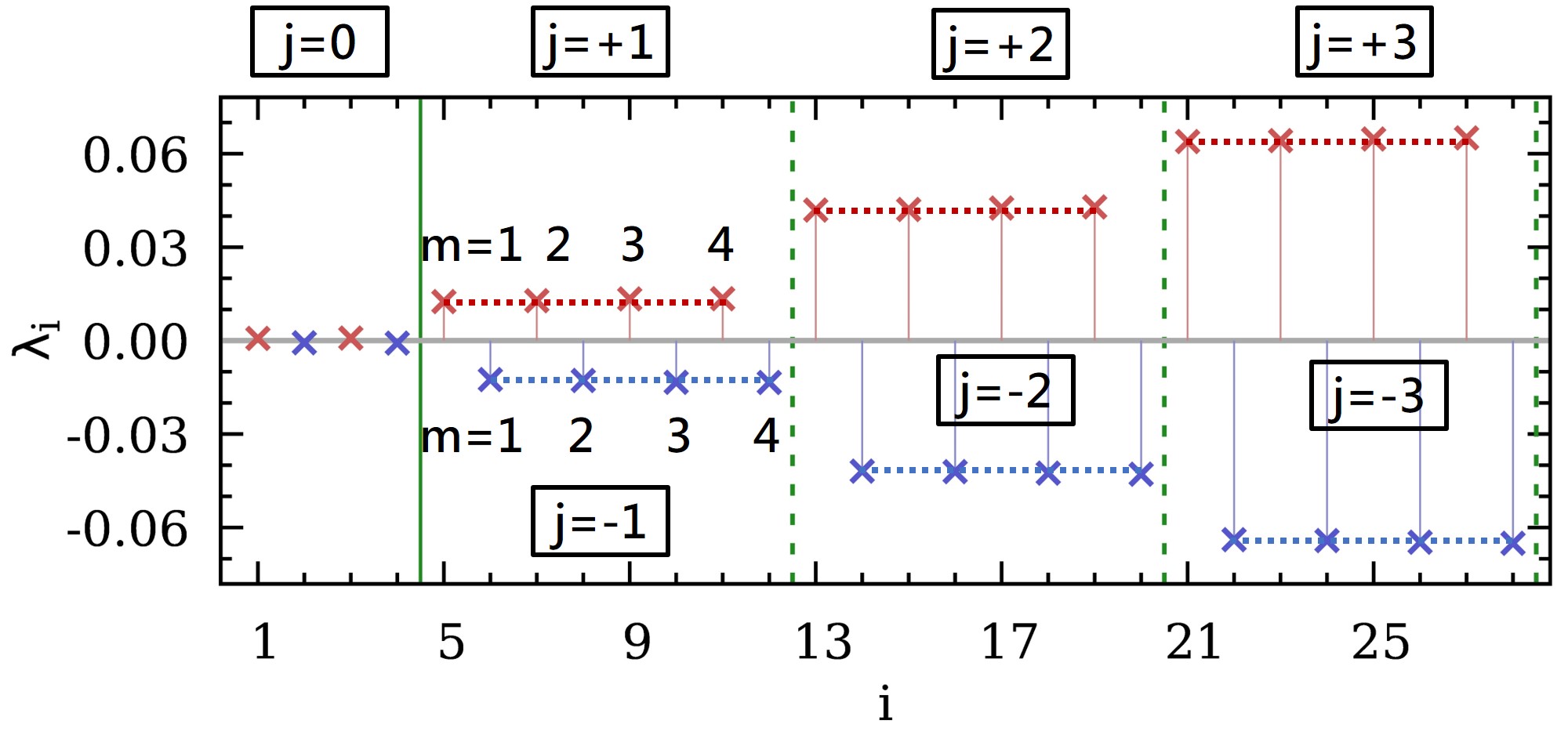
Figure 1: Staggered Dirac eigenvalue spectrum.

Let us describe the serial notation for Dirac eigenmodes. So far we have used a serial index $i$ for an eigenvalue $\lambda_{i}$ which is assigned in ascending order such that $i<j$ if $\lambda_{i}<\lambda_{j}$. It is convenient since we can use a compact notation such as $\Gamma_{5}^{i,k}$. Since the $SU(4)$ taste symmetry breaking effect is so small at $a\neq 0$, we can also introduce the quartet notation which reflects on the taste symmetry as in Figure 1. Here, we adopt the same quartet notation as in Ref. [4]:

$$D_{s}\lvert f_{j,m}\rangle=i\lambda_{j,m}\lvert f_{j,m}\rangle\equiv i\lambda_{j,m}\lvert j,m\rangle$$ (15)

where $j$ is a quartet index and $m$ is the index of a quartet component ($m=1,2,3,4$). In the continuum ($a=0$), $\lambda_{j,m}=\lambda_{j,n}$ for $m\neq n$ thanks to the $SU(4)$ taste symmetry. But on the lattice ($a>0$), $\lambda_{j,m}\neq\lambda_{j,n}$ for $m\neq n$ as one can see in Fig. 1. The ono-to-one mapping between a serial index $i$ and a quartet index $(j,m)$ is given in Table 1 for topological charge $Q=\pm 1$. Here, note that $\lambda_{2n-1}=-\lambda_{2n}$ for $n>0$, and $\lambda_{j,m}=-\lambda_{-j,m}$.

$\lambda_{i}$

$\lambda_{1}$

$\lambda_{2}$

$\lambda_{3}$

$\lambda_{4}$

$\lambda_{5}$

$\lambda_{7}$

$\lambda_{9}$

$\lambda_{11}$

$\lambda_{6}$

$\lambda_{8}$

$\lambda_{10}$

$\lambda_{12}$

$\cdots$

$\lambda_{j,m}$

$\lambda_{0,1}$

$\lambda_{0,2}$

$\lambda_{0,3}$

$\lambda_{0,4}$

$\lambda_{+1,1}$

$\lambda_{+1,2}$

$\lambda_{+1,3}$

$\lambda_{+1,4}$

$\lambda_{-1,1}$

$\lambda_{-1,2}$

$\lambda_{-1,3}$

$\lambda_{-1,4}$

$\cdots$

$i$

$1$

$2$

$3$

$4$

$5$

$7$

$9$

$11$

$6$

$8$

$10$

$12$

$\cdots$

$(j,m)$

$(0,1)$

$(0,2)$

$(0,3)$

$(0,4)$

$(+1,1)$

$(+1,2)$

$(+1,3)$

$(+1,4)$

$(-1,1)$

$(-1,2)$

$(-1,3)$

$(-1,4)$

$\cdots$

type

Z

Z

Z

Z

NZ

NZ

NZ

NZ

NZ

NZ

NZ

NZ

$\cdots$

Table 1: One-to-one correspondence between serial index $i$ and quartet index $(j,m)$ for $Q=\pm 1$. Here, Z (NZ) represents zero (non-zero) modes.

We find a minute deviation between eigenvalues within a quartet, $\lambda_{j,m}\neq\lambda_{j,n}$ for $m\neq n$ since the taste symmetry breaking is so tiny. We find that the size of taste symmetry breaking is only 7% even for the smallest non-zero quartet as one can see in Fig. 2.

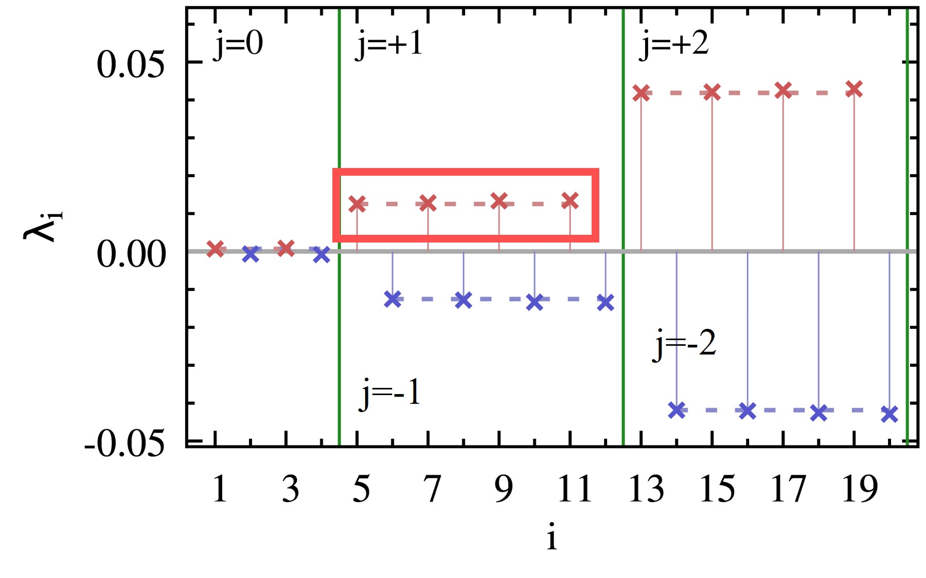
(a) A quartet structure

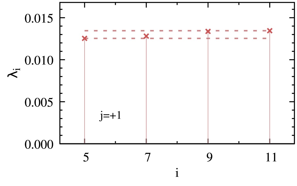
(b) A quartet structure for the smallest non-zero mode.

Figure 2: Examples for the quartet structure.

parameters	values
gluonic action	Tree level Symanzik and tadpole improvement [9, 10, 11]
lattice geometry	$20^{4}$
$a$	$0.077(1)$ fm
$\beta$	$5.0$
$N_{f}$	0 (quenched QCD)
number of gauge configurations	$300$
valence quarks	HYP staggered fermions [8]

Table 2: Details on gauge configuration [12].

5 Leakage pattern

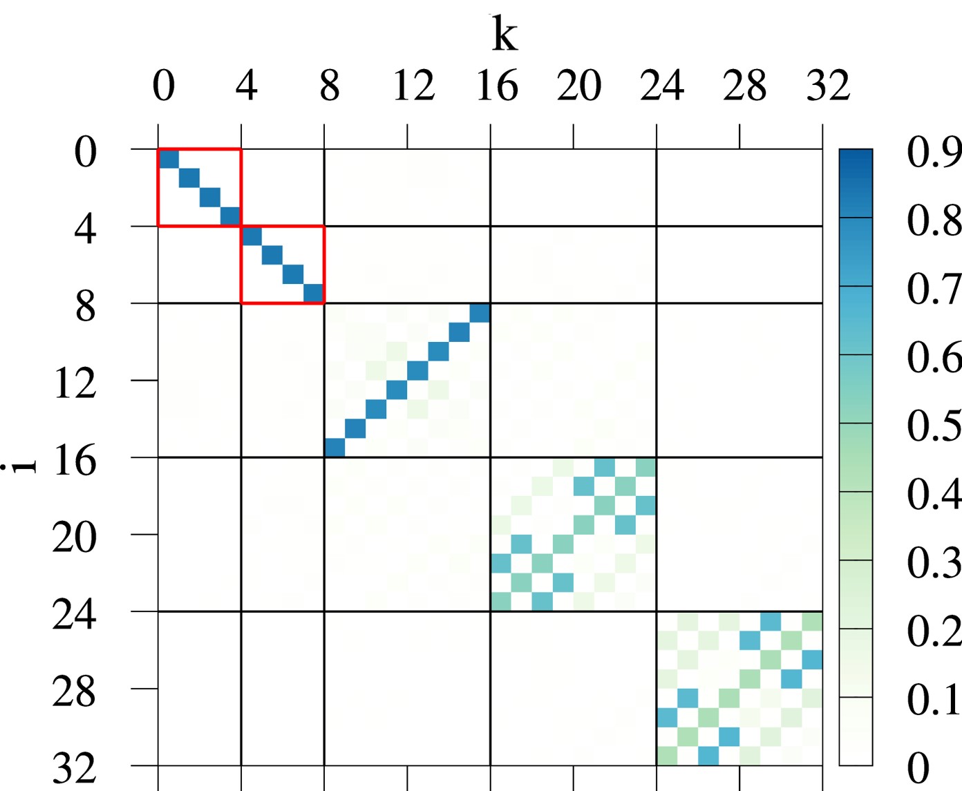
Figure 3: An example of leakage patterns.

First, let us consider the continuum case ($a=0$). A shift operator, which is also a generator for the $SU(4)$ taste symmetry, is

$$\Xi_{F}=[\mathbb{1}\otimes\xi_{F}]$$ (16)

where $\xi_{F}\in\{\xi_{5},\xi_{\mu},\xi_{\mu 5},\xi_{\mu\nu}\}$ (for $\mu\neq\nu$). Here, $\xi_{\mu}$ satisfies the Clifford algebra $\{\xi_{\mu},\xi_{\nu}\}=2\delta_{\mu\nu}$. Since the taste symmetry is conserved, $\Xi_{F}$ commutes with staggered Dirac operator,

$$0=\langle f_{i}\lvert[D_{s},\Xi_{F}]\rvert f_{k}\rangle=i(\lambda_{i}-\lambda_{k})|\Xi_{F}^{i,k}|~{}.$$ (17)

If $\lambda_{i}\neq\lambda_{k}$, $|\Xi_{F}^{i,k}|=\langle f_{i}\lvert\Xi_{F}\rvert f_{k}\rangle=0$. If $\lambda_{i}=\lambda_{k}$, $|\Xi_{F}^{i,k}|\neq 0$ is possible. $|\Xi_{F}^{i,k}|^{2}$ is a probability that one eigenstate transforms into another by $\Xi_{F}$. Hence, we call $|\Xi_{F}^{i,k}|$ the leakage parameter for the $\Xi_{F}$ operator. Here, note that the leakage by $\Xi_{F}$ can occur only within a quartet. And among the set of $\{\Xi_{F}\}$, $\Xi_{5}$ is especially important because it is related to $\Gamma_{5}$ by the Ward identity in Eqs. (12) and (13). Hence, $|\Gamma_{5}^{jm,-jn}|$ is just a mirror image of $|\Xi_{5}^{jm,jn}|$ for the non-zero modes ($j\neq 0$). Therefore, in the continuum ($a=0$),

$$\Gamma_{5}^{jm,\ell n}=\langle j,m\lvert\gamma_{5}\otimes\mathbb{1}\rvert\ell,n\rangle=\begin{cases}~{}\delta_{j\ell}\,\delta_{mn}&\text{for zero modes,}\\ ~{}\delta_{j,-\ell}\,\delta_{mn}&\text{for non-zero modes.}\end{cases}$$ (18)

On the lattice ($a\neq 0$),

$$\Gamma_{5}^{jm,\ell n}=\langle j,m\lvert\gamma_{5}\otimes\mathbb{1}\rvert\ell,n\rangle\simeq\begin{cases}~{}\delta_{j\ell}\,\delta_{mn}&\text{for zero modes,}\\ ~{}\delta_{j,-\ell}\,c_{mn}&\text{for non-zero modes,}\end{cases}$$ (19)

where $c_{mn}\neq 0$ due to the taste symmetry breaking. Hence, $|\Gamma_{5}^{i,k}|$ has a specific pattern which we call “ leakage pattern”. For zero modes it is diagonal within a quartet. For non-zero modes it is off-diagonal and non-trivial only between a quartet and its parity partner (we call them “octet” collectively because the parity partner can be determined from a quartet completely). Therefore, zero modes and non-zero modes can be distinguished by the leakage pattern. For example, we show a typical leakage pattern in Fig. 3. Here, the gauge configuration has $Q=+2$; $n_{-}=2$ (left-handed zero modes), $n_{+}=0$ (right handed zero modes). The chroma of blue color represents a value of $|\Gamma_{5}^{i,k}|$. Here, $i$ and $k$ are serial indices. The two red boxes represent two zero modes: one ($0\leq i\leq 3$) and the other ($4\leq i\leq 7$). We find that the leakage pattern for zero modes is diagonal within a quartet. There are three non-zero modes in Fig. 3. One represents $j=\pm 1$ ($8\leq i\leq 15$), another $j=\pm 2$ ($16\leq i\leq 23$), and the other $j=\pm 3$ ($24\leq i\leq 31$). The leakage pattern of non-zero modes is off-diagonal and random within an octet.

The leakage pattern (LP) method has a number of advantages compared with the spectral flow (SF) method [13]. First, the LP method is as robust as the SF method in identifying zero modes and non-zero modes. Second, the LP method is, at least by a factor of thousand, cheaper than the SF method in computational cost.

6 Deep learning study

Here, we want to address a question: Is the leakage pattern valid and universal over the entire gauge configurations? Since there are too many zero modes and non-zero modes with various $Q$ values, it is practically impossible to check the leakage pattern over the entire gauge configurations by analytic methods or by visual examination. Here, we introduce the deep learning (DL) techniques to solve the problem, which recognize a specific pattern embedded in the data if it exists, even though the data look completely random in the eye sight. The DL method allows us to check the leakage pattern for non-zero modes through the whole gauge configurations.

For the numerical study on the DL method, we use the lowest $200\times 200$ matrix elements of $|\Gamma^{i,k}_{5}|$ ($0\leq i,k<200$) on the lattice specified in Table 2.

6.1 Data sampling

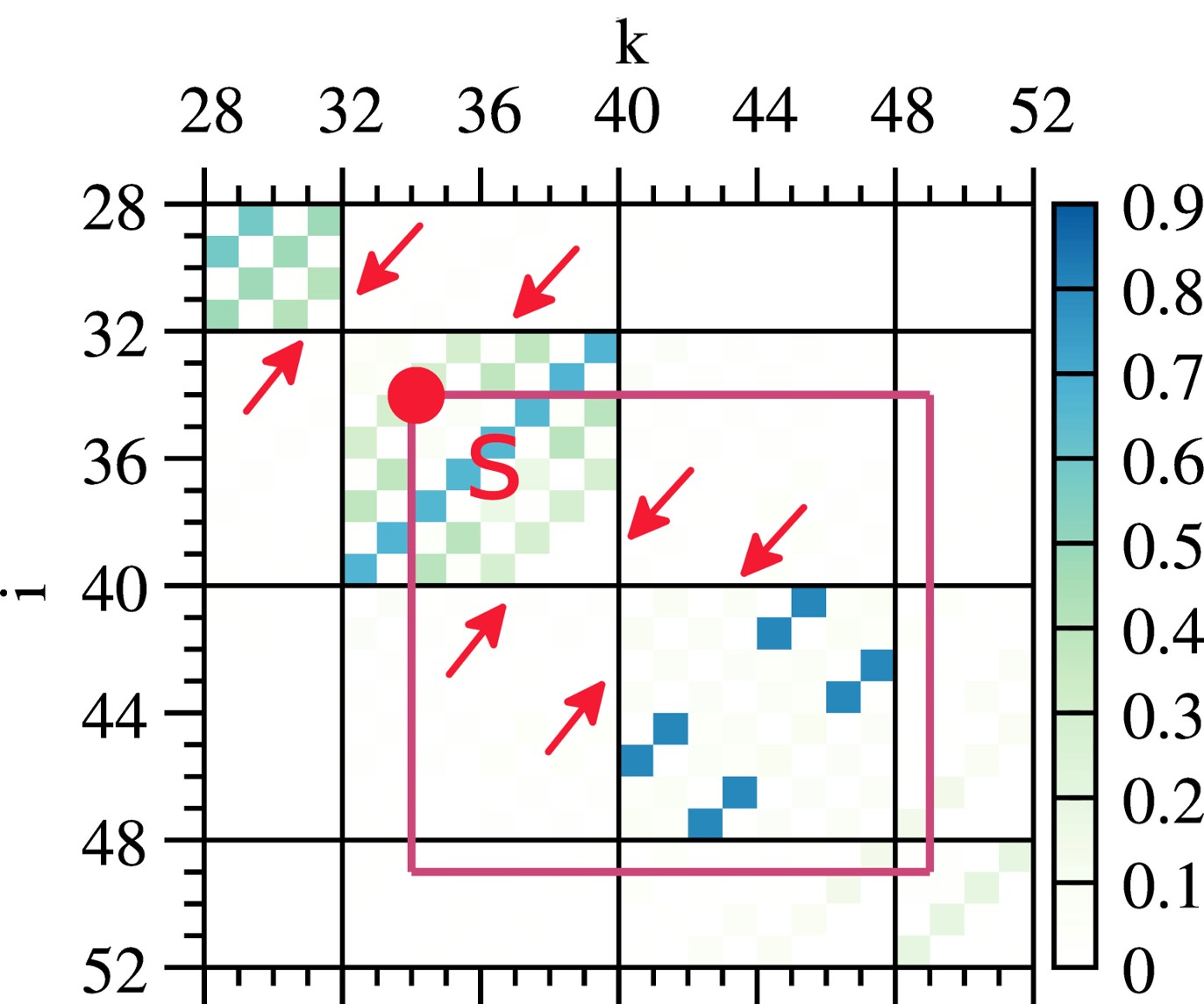
(a) Example for data sampling.

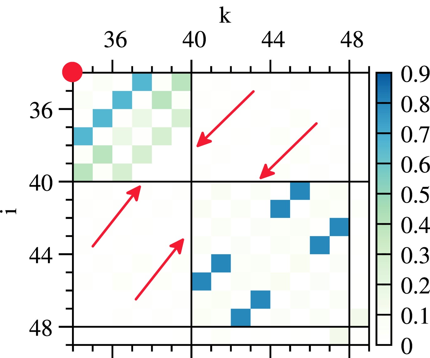
(b) A $15\times 15$ data sample (${\color[rgb]{1,0,0}s}=34$).

Figure 4: (4(b)) is a zoom-in version of the red square of (4(a)). The red square lines represent a typical data sample. The red blob in the upper left corner of the red square represents the sample serial index $s$ in Eq. (20). The red arrows point to the black border lines between non-zero mode octets.

Here, our task belongs to a classification problem in DL. We select $15\times 15$ sub-matrices randomly along the diagonal ($i=k$) line of the $200\times 200$ matrix of $|\Gamma^{i,k}_{5}|$. There is no overlap among the sub-matrices so that the probability distribution should be independent and identical. The sub-matrices are classified by the location of the border line between two adjacent octets as in Fig. 4, where an octet is composed of a quartet and its parity partner of non-zero modes. We choose the size of the sub-matrices as $15\times 15$ from the following guidelines.

• We want to maximize statistics or the number of samples, which requires minimizing the size of the sub-matrices.

• We want to make the whole samples contain at least one complete set of an octet.

The total number of different classes or labels (in terms of DL) is eight, which is equal to the number of components in an octet. We define the class ID, $C$ as follows,

$$C=(s-i_{b})\text{~{}mod }8$$ (20)

where $s$ is a serial index of the left-upper corner in a sub-matrix (e.g.  $i=k=34$, the red blob in Fig. 4(b)), and $i_{b}$ is a serial index for the border line (e.g.  $i=40$ and $k=40$, black lines in Fig. 4(b)). Examples for the eight classes are presented in Fig. $10$ of Ref. [4].

6.2 Deep learning analysis

DL model structure	our specific choice
Loss function	categorical cross-entropy
Hidden layer’s activation function	ReLU
Output layer’s activation function	Softmax
Optimization algorithm for loss function	Adam
Neural network layer	MLP, CNN, CNN + MLP
Auto-hyperparameter tuner	Keras tuner (random search)

Table 3: DL model structure

Details on the structure of our DL model are summarized in Table 3. Here, ReLU, MLP, and CNN represents rectified linear unit, multi layer Perceptron, and convolutional neural network, respectively. In order to perform the DL study, we need three types of data sets by construction: one for training, another for validation, and the other for test. Details on the DL data sets are given in Table 4(a).

data set	ngc	nds
training	120	1223
validation	30	308
test	142	1441

(a) DL data sets

layer	NN type	# of units	act.f.
input	-	225	-
1st hidden	MLP	160	ReLU
2nd hidden	MLP	1210	ReLU
3rd hidden	MLP	1490	ReLU
output	MLP	8	softmax

(b) The hyperparameters of the best performance model.

Table 4: DL data sets and the best performance model. (4(a)) The ngc (nds) represents the number of gauge configurations (the number of data samples). (4(b)) The NN denotes neural network and the act.f. activation function.

When we perform the auto hyperparameter tuning, we find out that our best performance model is MLP. The hyperparameters for MLP are given in Table 4(b). There are about ten samples ($15\times 15$ sub-matrices) per gauge configuration as shown in Table 4(a). We adopt the accuracy metric to measure the performance of DL model. The accuracy is defined as a ratio $TC/TND$, where $TC$ represents the number of truly classified samples (DL prediction is equal to true class), and $TND$ represents the total number of the data samples.

In the test data set, we find that there are two independent sets of gauge configurations which are distinct by the accuracy: one set of five gauge configurations has accuracy less than 0.5, and the other set of 137 gauge configurations has accuracy of about 0.9. The former are called “abnormal set” and the latter “normal set”. The abnormal gauge configurations are entirely caused by the ghost eigenvalue problem of Lanczos algorithm [14]. Before we begin our numerical study on the DL method, we have excluded by hand those abnormal gauge configurations on which the topological charge $Q$ measured by the index theorem is different from that of the direct measurement. In fact, the DL method is the best to identify the abnormal gauge configurations such that we can filter them out.

Let us consider the accuracy $A_{i}$ measured on a gauge configuration with an index $i$. Then we can consider a set of the accuracies $S_{a}=\{A_{i}\}$ for $1\leq i\leq N$. We also have a set of the number of samples $M_{i}$ for each gauge configuration $S_{n}=\{M_{i}\}$. Then we can consider an weighted average of the accuracy $\bar{A}$ over the gauge configurations:

$$\bar{A} =\frac{\sum\limits_{i}M_{i}A_{i}}{\sum\limits_{i}M_{i}}\,, \sigma_{\bar{A}}^{2}=\frac{\sum\limits_{i}M_{i}(A_{i}-\bar{A})^{2}}{(N-1)\sum\limits_{i}M_{i}}\,,$$ (21)

where $\sigma_{\bar{A}}$ is the statistical error for $\bar{A}$. In Table 5, we present results for $\bar{A}$ measured over the entire set (mixed = normal + abnormal), a subset of the abnormal gauge configurations (abnormal), and a subset of the normal gauge configurations (normal). The accuracy for the abnormal subset is so small that the DL method can identify it easily. We find that the large error for the mixed set comes from that for the abnormal subset. We also find that the extremely high accuracy for the normal subset reflects on the fact that the DL method succeeds in classifying the samples of the normal subset, which leads to the key point that if we select the majority of the DL prediction on each gauge configuration, we can distinguish all the non-zero mode octets perfectly over the entire normal subset.

We apply the DL method on the non-zero modes, because they are more appropriate for the DL analysis due to the following reasons: 1) abundant data, 2) complex structure, and 3) randomness in leakage pattern. The DL analysis gives a border line of the non-zero modes octets robustly. The leakage pattern for zero modes combined with the DL method is as robust as the SF method in determining the topological charge $Q$. However the key point is that the computational cost for the DL method is much cheaper than the SF method by at least a factor of 1000.

configuration	# conf.	$\bar{A}$ [%]
mixed	142	$96.5(13)$
abnormal	5	$17.3(78)$
normal	137	$99.4(2)$

Table 5: Results for the accuracy $\bar{A}$ for mixed, abnormal, and normal set of gauge configurations in the test data set.

6.3 ROC curve

In the previous subsection, we use the accuracy metric for the DL analysis. In general, for a skewed probability distribution of classes, the accuracy is not such a good metric that it might give a misleading information on the DL model performance [15]. Since the class distribution of our data samples is not skewed but uniform, the accuracy is a good metric for our DL analysis. There are tens of alternative metrics in the DL market. Among them, the AUC (area under ROC curve) [16] is one of the most popular metrics, and can be used instead of accuracy even if the class distribution is skewed. Here, the ROC stands for receiver operating characteristic. In order to crosscheck results from the accuracy metric, we adopt the AUC metric, even though we expect that both metrics will give the same answer for our data sets in the end of day.

A ROC curve is defined in binary class (positive and negative classes). As in Fig. 5, $y$-axis of ROC curve is true positive rate (TPR) and $x$-axis is false positive rate (FPR).

TPR $$=\frac{TP}{P} \text{FPR}=\frac{FP}{N}$$ (22)

Here, $TP$ ($FP$) represents the number of the samples for which the DL prediction is positive and their actual class is positive (negative). The $P$ ($N$) is the total number of samples in the actual positive (negative) class. Here, the DL binary model gives a probability that each sample belongs to the positive class. The DL model prediction for each sample is determined by a threshold applied to the probability to accept it (positive prediction) or reject it (negative prediction). The number of samples in the positive prediction changes according to the threshold value, and so do the $TP$ and $FP$, which leads to a corresponding change in TPR and FPR. Hence, we may obtain the ROC curve for the DL binary model by running the threshold from 0 to 1.

If we set the threshold to zero, all the predictions by the DL binary model are positive, which results in a trivial case that $TP=P$ and $FP=N$, which corresponds to $(1,1)$ in the ROC curve. If the threshold is set to 1, all the preditions are negative, which makes $TP=0$ and $FP=0$, which corresponds to $(0,0)$ in the ROC curve. Hence, the ROC curves, in general, share the two points $(1,1)$ and $(0,0)$ in common. If the DL predictions are perfect (i.e. $TP=P$ and $FP=0$), then the ROC curve passes through $(1,0)$. AUC is the area under the ROC curve, and so AUC for a perfect DL model is 1. If the DL predictions are random (i.e. $TP=0.5P$ and $FP=0.5N$), the ROC curve corresponds to the blue dashed line in Fig. 5, which makes AUC=0.5. Hence, AUC is an alternative good metric for the DL model performance. If the DL model prediction gets better, its AUC becomes closer to 1. If the DL model prediction gets worse, its AUC becomes closer to 0.5.

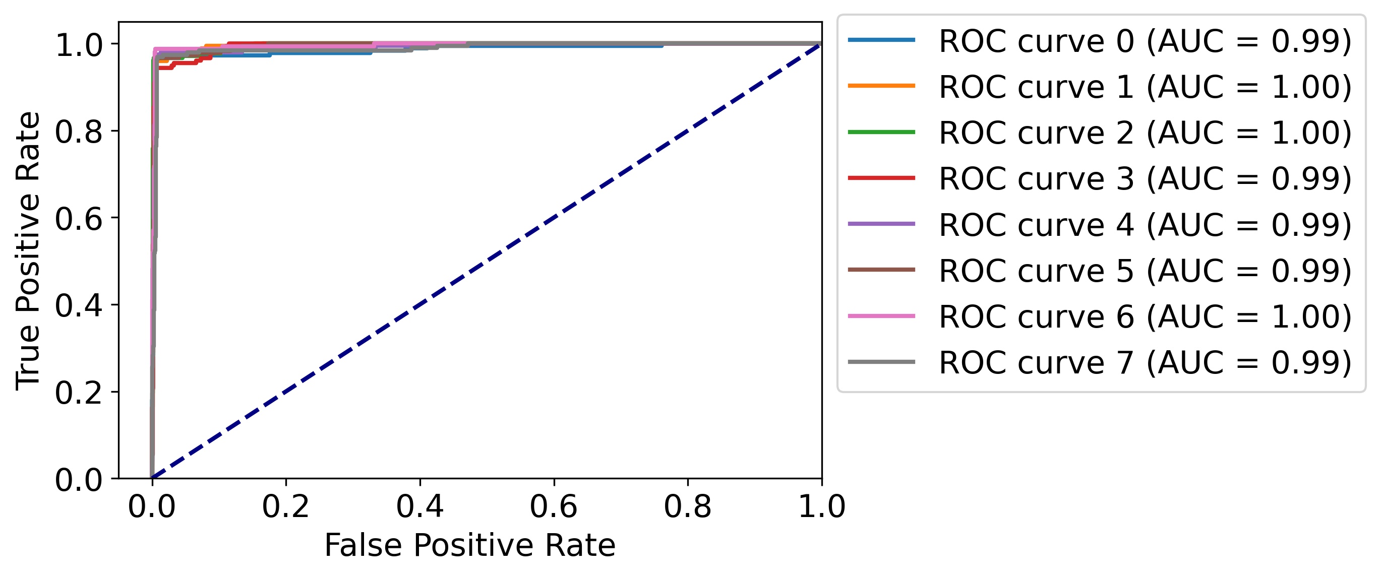
Figure 5: ROC curves and AUC metric for our best performance model

Since our DL model belongs to the multiclass classification, we need to extend the binary-class picture of the ROC curve to the multiclass picture. We use the one-versus-rest method to extend the ROC curve to the multiclass classification [16, 17]. The one-versus-rest method converts multiclass classification into binary class classification regarding $c_{i}$ as a positive class and the rest ($\{c_{j}|j\neq i\}$) as a negative class. In Fig. 5, we present the ROC curve and its AUC($c_{i}$) for each class $c_{i}$ in our best DL model. Our total AUC is

$$\text{AUC}_{\text{tot}}=\frac{\sum\limits_{c_{i}\in\,C}\text{AUC}(c_{i})w(c_{i})}{\sum\limits_{c_{i}\in\,C}w(c_{i})}$$ (23)

where $C$ is a set of all classes, and $w(c_{i})$ is a weight of $c_{i}$ (= the number of samples in $c_{i}$). Our best performance model (MLP) gives $\text{AUC}_{\text{tot}}=0.998\simeq 1$ for the normal set.

The $\text{AUC}_{\text{tot}}$ value implies that our best DL model works almost perfectly. Results for the AUC metric are highly consistent with those for the accuracy metric in the previous subsection. Its physical meaning is that the leakage pattern for zero and non-zero modes is universal over the normal gauge configurations.

7 Conclusions

Thanks to the $U(1)_{A}$ symmetry and the $SU(4)$ taste symmetry, the leakage pattern (LP) for zero modes is quite different from that for non-zero modes. We use the deep learning (DL) method to verify that the LPs for the chirality operator are universal over the normal gauge configurations, which we can not prove analytically nor visually. We find that, using the LP method combined with the DL method, we can determine topological charge as robustly as the spectral flow (SF) method. Since the computational cost for the LP/DL method is much cheaper than that for SF at least by a factor of 1000, the LP/DL method is highly promising.

References

- [1] N. D. Cundy, H. Jeong, and W. Lee, Calculation of strange and light quark condensate using improved staggered fermions and overlap fermions, PoS LATTICE2015 (2016) 066.
- [2] SWME Collaboration, H. Jeong, S. Jwa, J. Kim, S. Kim, S. Lee, W. Lee, and J. Pak, How to identify zero modes for improved staggered fermions, in 35th International Symposium on Lattice Field Theory, 11, 2017. 1711.01826.
- [3] SWME Collaboration, H. Jeong, S. Kim, W. Lee, J. Pak, and C. Jung, Chiral Ward identities for Dirac eigenmodes with staggered fermions, PoS LATTICE2019 (2020) 031, [2001.06568].
- [4] SWME Collaboration, H. Jeong et al., Chiral symmetry and taste symmetry from the eigenvalue spectrum of staggered Dirac operators, Phys. Rev. D 104 (2021), no. 1 014508, [2005.10596].
- [5] J. Smit and J. C. Vink, Remnants of the Index Theorem on the Lattice, Nucl. Phys. B 286 (1987) 485–508.
- [6] M. F. L. Golterman and J. Smit, Selfenergy and Flavor Interpretation of Staggered Fermions, Nucl. Phys. B 245 (1984) 61–88.
- [7] H. Kluberg-Stern, A. Morel, O. Napoly, and B. Petersson, Flavors of Lagrangian Susskind Fermions, Nucl. Phys. B 220 (1983) 447–470.
- [8] A. Hasenfratz and F. Knechtli, Flavor symmetry and the static potential with hypercubic blocking, Phys. Rev. D 64 (2001) 034504, [hep-lat/0103029].
- [9] M. Luscher and P. Weisz, On-Shell Improved Lattice Gauge Theories, Commun. Math. Phys. 97 (1985) 59. [Erratum: Commun.Math.Phys. 98, 433 (1985)].
- [10] M. G. Alford, W. Dimm, G. P. Lepage, G. Hockney, and P. B. Mackenzie, Lattice QCD on small computers, Phys. Lett. B 361 (1995) 87–94, [hep-lat/9507010].
- [11] G. P. Lepage and P. B. Mackenzie, On the viability of lattice perturbation theory, Phys. Rev. D 48 (1993) 2250–2264, [hep-lat/9209022].
- [12] HPQCD, UKQCD Collaboration, E. Follana, A. Hart, C. T. H. Davies, and Q. Mason, The Low-lying Dirac spectrum of staggered quarks, Phys. Rev. D 72 (2005) 054501, [hep-lat/0507011].
- [13] D. H. Adams, Theoretical foundation for the Index Theorem on the lattice with staggered fermions, Phys. Rev. Lett. 104 (2010) 141602, [0912.2850].
- [14] J. Cullum and R. A. Willoughby, A survey of lanczos procedures for very large real ‘symmetric’ eigenvalue problems, Journal of Computational and Applied Mathematics 12-13 (1985) 37–60.
- [15] P. Branco, L. Torgo, and R. P. Ribeiro, A survey of predictive modeling on imbalanced domains, ACM Comput. Surv. 49 (2016), no. 2.
- [16] T. Fawcett, An introduction to roc analysis, Pattern Recognition Letters 27 (2006), no. 8 861–874. ROC Analysis in Pattern Recognition.
- [17] F. Provost and P. Domingos, Well-trained pets: Improving probability estimation trees, 2000.