Nonlinear Kernel Support Vector Machine with 0-1 Soft Margin Loss

Abstract

Recent advance in linear support vector machine with the 0-1 soft margin loss ($L_{0/1}$-SVM) shows the probability of solving the 0-1 loss problem directly. However, its theoretical and algorithmic requirements restrict us from directly extending the linear solving framework to its nonlinear kernel form. The lack of an explicit expression of the Lagrangian dual function of $L_{0/1}$-SVM is a major shortcoming among them. By applying the nonparametric representation theorem, we propose a nonlinear model for support vector machine with 0-1 soft margin loss, called $L_{0/1}$-KSVM, which skillfully incorporates the kernel technique, and more importantly, follows the success in systematically solving its linear problem. The optimal condition is theoretically explored and a working set selection alternating direction method of multipliers (ADMM) algorithm is introduced to obtain its numerical solution. Furthermore, we first introduce a closed-form definition to the support vector (SV) of $L_{0/1}$-KSVM. Theoretically, we prove that all SVs of $L_{0/1}$-KSVM are only located on the parallel decision surfaces. The experimental results show that $L_{0/1}$-KSVM has much fewer SVs compared to its linear counterpart and the other six nonlinear benchmark SVM classifiers, while maintaining good prediction accuracy.

1 Introduction

Vapnik and Cortes first proposed the support vector machine (SVM) for binary classification in 1995 [1], then it became a very popular modelling and prediction tool for many small and moderate scale machine learning, statistic and pattern recognition problems [2]. The SVM classifier aims to build a linear or nonlinear maximum-margin decision boundary to separate two classes of data points. Usually, the nonlinear SVM model is preferred in most practical scenarios [3]. Given a data set ${\mathcal{X}}\times{\mathbb{Y}}=\{(\textbf{x}_{1},y_{1}),(\textbf{x}_{2},y_{2}),~{}\ldots~{},(\textbf{x}_{m},y_{m})\}\subseteq\mathbb{R}^{n}\times\{{+1},{-1}\}$, here $y_{i}\in\mathbb{Y}=\{{+1},{-1}\}$$(i\in{\mathbb{N}}_{m},{\mathbb{N}}_{m}:=1,~{}\cdots~{},m)$ is the label value corresponding to input $\textbf{x}_{i}\in{\mathbb{R}}^{n}(i\in{\mathbb{N}}_{m})$, the formulation of the nonlinear SVM problem is

$$\underset{\textbf{w}\in{\mathbb{R}}^{n},b\in\mathbb{R}}{\min} \frac{1}{2}\|\textbf{w}\|^{2}+C\sum_{i=1}^{m}\ell(1-y_{i}f(\textbf{x}_{i}))$$

where $C>0$ is a penalty parameter and the decision surface ${f}(\cdot)$ is defined by ${f}({\textbf{x}})=\left\langle{\textbf{w}},\Phi(\textbf{x})\right\rangle+b=0$, $\Phi(\cdot)$ is an appropriate feature map that expects new higher-dimensional points $\Phi(\textbf{x})(\textbf{x}\in{\mathcal{X}})$ linearly separable in the feature space. The loss function $\ell(\cdot)$ measures the penalty on the misclassified data points $\{\textbf{x}_{i}\bigg{|}1-y_{i}f(\textbf{x}_{i})>0,i\in{\mathbb{N}}_{m}\}$. The 0-1 loss function $\ell_{0/1}(\cdot)$ is a natural option of $\ell(\cdot)$ since it captures the discrete nature of binary classification, i.e., it is designed to minimize the number of misclassified instances

$$\ell_{0/1}(u_{i})=\begin{cases}1,&u_{i}>0,\\ 0,&u_{i}\leq 0,\end{cases}$$

here $u_{i}=1-y_{i}f(\textbf{x}_{i}),i\in{\mathbb{N}}_{m}$. However, its non-convexity and discontinuity make the problems with 0-1 loss NP-hard to optimize [4-7]. For decades, compromising with the challenge of directly solving the original SVM with 0-1 loss, many researchers transfer to operate the following two alternative strategies instead: replacing the 0-1 loss function with surrogate loss functions, or executing approximate algorithms based on the binary-valued property of 0-1 loss function.

In the SVM community, a tremendous amount of work has been devoted to the first strategy, in particular to SVMs with convex surrogates because of their ease-of-use in practical applications and their convenience in theoretical analyses. However, there is no solid evidence on how well these convex surrogates approximate the 0-1 loss itself, even if they have asymptotic relevance [8]. Among the most widely researched surrogates are hinge loss [1], least squares loss [9], squared hinge loss [10], pinball loss [11] and log loss [12]. Compared to convex surrogates, ramp loss [13,14], the rescaled hinge loss [15], the non-convex and smooth loss [16] (See Figure 1), etc, these non-convex surrogates still attract much attention in certain scenes requiring high insensitivity to outliers. At the same time, these non-convex SVMs show relatively better performance in classification accuracy and the SVs decline. As for the majority of nonlinear SVMs with convex surrogates, their optimization problems can be systematically researched by the dual kernel-based technique combined with KKT condition. Unfortunately, this method cannot guarantee the same success for many non-convex surrogates. With respect to the 0-1 loss, the ideal candidate for SVM loss, we find it is challenging to implement the Lagrangian dual approach directly. The reason is that the core function, namely, the Lagrangian dual function of the 0-1 loss SVM can not be explicitly expressed due to the non-smoothness and non-convexity of 0-1 loss function. Finally, the failure of this popular technique, also the lack of other effective ways to directly solve this NP-hard problem makes the task of exactly solving the 0-1 loss SVM a decades-long challenge in the SVM community.

As for the second strategy, some approximate algorithms used sigmoid function [17] or a sigmoidal transfer function [18] as the simulation of 0-1 loss for their similar numerical characteristics. Moreover, Orsenigo and Vercellis [19] proposed the algorithm of multivariate classification trees based on minimum features discrete support vector machines and an approximate technique was performed to solve the mixed integer problem (MIP) model at each node of trees in their method. A point must be acknowledged that these approximate algorithms mainly focus on techniques other than systematic solving framework including sound theoretical analysis, such as proposing an optimal condition, and the solving algorithm more closely adhering to the SVM problems.

Most lately, Wang et al. [20] have made a great step in their systematic work aimed at directly solving the linear $L_{0/1}$-SVM, an abbreviation for the linear SVM with 0-1 loss. To the best of our knowledge, they first built the optimal condition for both the global and local solutions of the linear $L_{0/1}$-SVM by virtue of proximal operator of 0-1 loss function, and then an efficient algorithm $L_{0/1}$-ADMM was invented to find the approximate solution based on the optimal condition. In view of the fundamental or theoretical achievements on directly solving the SVM with 0-1 loss are not yet fully developed, the relatively systematic work on linear $L_{0/1}$-SVM in [20] is a meaningful attempt on this topic. Therefore, we expect that their inspiring view can lead us to build a similar systematic framework for nonlinear $L_{0/1}$-SVM.

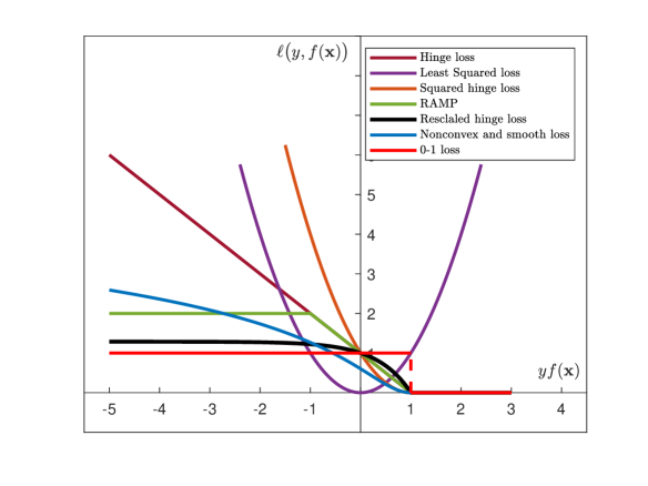
Figure 1: The 0-1 loss function and other common loss functions.

A powerful and popular method for dealing with the nonlinear SVMs is the kernel method [9][21]. In general, most nonlinear SVM problems need to incorporate the kernel technique into their Lagrangian dual functions. As mentioned earlier, the explicit formulation of the Lagrangian dual function of $L_{0/1}$-SVM is unaccessible because the 0-1 loss function has the negative property of convexity and continuity. The dilemma forces researchers to explore other ways that can still effectively use kernel trick but without involving the surrounding of the Lagrangian dual problem. One way is to approximate the kernel function by proper feature map. The technique for speeding up kernel methods on large-scale problems, called the class of random features [22,23], is of this type. Specifically, it approximately decomposes the kernel function by using a explicit feature map and then transforms the nonlinear SVM problems into the linear case.

In this paper, based on the nonparametric representation theorem [24], a nonlinear $L_{0/1}$-SVM model, called $L_{0/1}$-KSVM is presented. The new $L_{0/1}$-KSVM model skillfully incorporates the kernel technique without using the Lagrangian dual function. More importantly, the proposed model also successfully extend the systematic solving framework of linear model in [20], in other words, the corresponding optimal condition and algorithm are similarly explored, as the linear framework was completed in [20]. The main contributions can be summarized as follows.
(i) A new formulation of the nonlinear kernel $L_{0/1}$-SVM, called $L_{0/1}$-KSVM, is presented. The new proposed $L_{0/1}$-KSVM simultaneously incorporates the kernel technique and adopts the advanced and systematic solving framework of $L_{0/1}$-SVM. Moreover, we prove that the $L_{0/1}$-KSVM model degenerates into a slightly modified edition of the original linear $L_{0/1}$-SVM by adding an extra regularization $\frac{1}{2}b^{2}$ into its objective function.
(ii) A precise definition of the support vector and the optimality condition of the $L_{0/1}$-KSVM are given by the proximal constraints of P-stationary point and an important conclusion about SVs is also explored: SVs are only located on the parallel decision surfaces ${f(\cdot)}=\pm 1$, where ${f(\cdot)}=0$ is the final decision surface. This geometric character relating to SVs echoes the fact that SVMs with 0-1 loss has much smaller SVs than other SVM peers with traditional convex losses.
(iii) The experimental part, respectively using $L_{0/1}$-SVM and the other six classical nonlinear SVMs for performance comparison, has validated the strong sparsity and reasonable robustness of our proposed $L_{0/1}$-KSVM. The result of much fewer SVs of the $L_{0/1}$-KSVM is in stark contrast to all other experimental counterparts. Meanwhile, we have achieved a decent result in terms of prediction accuracy compared to the other six classical nonlinear SVMs.

The rest of the paper is organized as follows. Section 2 gives a broad outline for the $L_{0/1}$-SVM and then presents two foundations for modelling the nonlinear $L_{0/1}$-KSVM, the kernel method and the representation theorem. The whole framework of $L_{0/1}$-KSVM, which is also the topic of the current paper, is explicitly studied in section 3. Finally in section 4, we will prove the advantageous aspects of $L_{0/1}$-KSVM on strong sparsity and robustness through experiments compared to the $L_{0/1}$-SVM and the other six classical nonlinear SVMs.

2 Preliminary knowledge

First, we give a brief overview on linear $L_{0/1}$-SVM; then the following part focuses on presenting the knowledge about the kernel method and the representation theorem, which are crucial for building our final model $L_{0/1}$-KSVM. For convenience, some notations are given in Table 1.

Table 1: List of notations.

Notation	Description
X	$[\textbf{x}_{1}\ \textbf{x}_{2}\ldots\ \textbf{x}_{m}]^{\top}\in\mathbb{R}^{m\times n}$
$A$	$[y_{1}\textbf{x}_{1}~{}y_{2}\textbf{x}_{2}~{}\ldots~{}y_{m}\textbf{x}_{m}]^{\top}\in\mathbb{R}^{m\times n}$
y	$(y_{1},y_{2},\ldots,y_{m})^{\top}\in\mathbb{R}^{m}$
$\widetilde{A}$	$[A,\textbf{y}]\in\mathbb{R}^{m\times(n+1)}$
V	$\text{Diag}(\textbf{y})=\text{Diag}(y_{1},y_{2},\ldots,y_{m})\in{\mathbb{R}}^{m\times m}$
e	$(1,1,\ldots,1)^{\top}\in{\mathbb{R}}^{m}$
${\widetilde{{A}}}^{+}$	$({\widetilde{{A}}}^{\top}{\widetilde{{A}}})^{-1}{\widetilde{{A}}}^{\top}\in{\mathbb{R}}^{(n+1)\times m}$
$H$	$\begin{bmatrix}I_{n\times n}&{\bf 0}\\ {\bf 0}&0\\ \end{bmatrix}{\widetilde{{A}}}^{+}\in{\mathbb{R}}^{(n+1)\times m}$, here ${\bf 0}\in{\mathbb{R}}^{n}$
$t_{+}$	$\text{max}\{t,0\},t\in{\mathbb{R}}$
u	$(u_{1},u_{2},\ldots,u_{m})^{\top}\in{\mathbb{R}}^{m}$
${\textbf{u}}_{+}$	$((u_{1})_{+},\ldots,(u_{m})_{+})^{\top}\in{\mathbb{R}}^{m}$
$\|\textbf{u}\|_{0}$	The number of non-zero elements in u

2.1 Linear $L_{0/1}$-SVM

We now give a simple overview related to the $L_{0/1}$-SVM by Wang and his partners in [20]. First, they rewrote the SVM with 0-1 loss into the following matrix form

$$\begin{split}\underset{\textbf{w}\in{\mathbb{R}}^{n},b\in\mathbb{R},{\textbf{u}}\in{\mathbb{R}}^{m}}{\min}&~{}~{}\frac{1}{2}\|\textbf{w}\|^{2}+C\|{\textbf{u}}_{+}\|_{0}\\ \mbox{s.t.\ }&~{}~{}{\textbf{u}}+A\textbf{w}+b\textbf{y}={\textbf{e}},\end{split}$$ (1)

and the hyperplane or decision function is of the form ${f}({\textbf{x}})=\left\langle{\textbf{w}},{\textbf{x}}\right\rangle$+$b$. Note that u is obtained here under the condition that $\Phi$ is an identity map.

The optimal condition of (1) was presented in Theorem 1, which was introduced by an important concept, the P-stationary point. We will review them respectively in the following part:

Definition 1

[20][P-stationary point of (1)] For a given $C>0$, we say $({\textbf{w}^{*}};b^{*};\textbf{u}^{*})$ is a proximal stationary (P-stationary) point of (1) if there are a Lagrangian multiplier vector ${\boldsymbol{\lambda}^{*}}\in\mathbb{R}^{m}$ and a constant $\gamma>0$ such that

$$\left\{\begin{array}[]{rll}\textbf{w}^{*}+A^{\top}{\boldsymbol{\lambda}^{*}}&={\bf 0},\\ \langle\textbf{y},{\boldsymbol{\lambda}^{*}}\rangle&={\bf 0},\\ {\textbf{u}}^{*}+A\textbf{w}^{*}+b^{*}\textbf{y}&={\textbf{e}},\\ \text{Prox}_{\gamma C\|({\cdot})_{+}\|_{0}}(\textbf{u}^{*}-\gamma{\boldsymbol{\lambda}^{*}})&=\textbf{u}^{*},\end{array}\right.$$ (2)

where

$$[\text{Prox}_{\gamma C\|({\cdot})_{+}\|_{0}}({\textbf{z}^{*}})]_{i}=\begin{cases}0,&0<z^{*}_{i}\leq\sqrt{2\gamma C},\\ z^{*}_{i},&z^{*}_{i}>\sqrt{2\gamma C}~{}\text{or}~{}z^{*}_{i}\leq 0.\end{cases}$$ (3)

Here, $\textbf{z}^{*}:=\textbf{u}^{*}-\gamma{\boldsymbol{\lambda}^{*}}$.

Theorem 1

[20] For problem (1), the following relations hold.

(i)  Assume $\widetilde{{A}}$ has a full column rank. For a given $C>0$, if $(\textbf{w}^{*};b^{*};{\textbf{u}^{*}})$ is a global minimizer of (1), then it is a P-stationary point of (1) with $0<\gamma<1/\lambda_{H}$, where $\lambda_{H}$ represents the maximum eigenvalue of $H^{\top}H.$

(ii) For a given $C>0$, if $(\textbf{w}^{*};b^{*};{\textbf{u}^{*}})$ is a P-stationary point of (1) with $\gamma>0$, then it is a local minimizer of (1).

The theorem states that the P-stationary point must be a local minimizer under a certain condition, and [20] used the P-stationary point as a termination rule for the iterative points generated by $L_{0/1}$-ADMM, the algorithm for numerically solving (1). In addition, they introduced a new expression to the SV based on P-stationary point and further verified that SVs lie only on the parallel decisive hyperplanes ${f}({\textbf{x}})=\left\langle{\textbf{w}},{\textbf{x}}\right\rangle$+$b=\pm 1$, which was expected to guarantee the high efficiency because of its strong sparsity and relative robustness due to its insensitivity to outliers.

In [20], the $L_{0/1}$-SVM in theory and experiment has shown the great advantage of rather a shorter computation time and many fewer SVs compared to other leading linear SVM classifiers. However, we point out some obstacles when we extend the whole efficient modelling framework from the linear form to the nonlinear form.
(i). Theoretically, the number of the representation of the nonlinear or kernel basis is always larger than the number of training points. Therefore, the requirement that the full column rank of $\widetilde{{A}}$ in Theorem 1 in [20] cannot be satisfied if we normally introduce nonlinear mapping or kernel trick to handle the nonlinear SVM problems.
(ii). Algorithmically, $L_{0/1}$-ADMM, designed to solve linear $L_{0/1}$-SVM, requires data points $\mathcal{X}$ explicitly expressed in the iteration of w and it is hampered by the fact that in most cases we do not know ${\Phi(\mathcal{X})}$ but their product dots.

To overcome these challenges, we seek a new nonlinear model suitable for the entire linear framework just reviewed, the following subsection will provide the essential basis to construct it.

2.2 Kernel Method and Representation Theorem

In the kernel method, the kernel function plays a central role and the representation theorem is also closely related to the kernel function, since it is the basic element to construct the Hilbert space in which the representation theorem holds.

When failing to find a hyperplane as to the linearly inseparable data points $x_{i}\in{\mathcal{X}}(i\in{\mathbb{N}}_{m},\mathcal{X}\subseteq\mathbb{R}^{n})$, an ingenious solution is that we can transfer the original data set ${\mathcal{X}}$ into a new separable domain $\Phi({\mathcal{X}})$, here $\Phi({\mathcal{X}})$ is always a subset of dot product space ${\mathscr{H}}$ under the proper mapping $\Phi$. Since most nonlinear SVMs algorithms need to know only the dot products of the new domain $\Phi({\mathcal{X}})$ but not $\Phi({\mathcal{X}})$ themselves. Furthermore, ${\mathscr{H}}$ is high dimensional, sometimes even with $\infty$, then a new technique called kernel method is introduced to alleviate the computation burden in ${\mathscr{H}}$. The kernel function, playing a key role in this method, is defined as follows:

Definition 2 (Kernel function)

[25] For a given binary function $k:{\mathcal{X}}\times{\mathcal{X}}\rightarrow\mathbb{R}$, $({\textbf{x}_{i}},{\textbf{x}_{j}})\mapsto k({\textbf{x}_{i}},{\textbf{x}_{j}})$, there exists a map $\Phi$ from ${\mathcal{X}}$ to a dot product space ${\mathscr{H}}$, for all ${\textbf{x}_{i}},{\textbf{x}_{j}}\in{\mathcal{X}}$, satisfying $k({\textbf{x}_{i}},{\textbf{x}_{j}})=\langle\Phi({\textbf{x}_{i}}),\Phi({\textbf{x}_{j}})\rangle$, then function $k(\cdot,\cdot)$ is usually called kernel function and $\Phi(\cdot)$ is called its feature map.

The most frequently used kernel function includes Polynomial kernel function [26] $k({\textbf{x}},{\textbf{x}}^{{}^{\prime}})={\langle{\textbf{x}},{\textbf{x}}^{{}^{\prime}}\rangle}^{d}$ $({d}\geq 1)$, Gaussian kernel function [27,28] $k({\textbf{x}},{\textbf{x}}^{{}^{\prime}})=\exp(-\frac{\|{\textbf{x}}-{\textbf{x}}^{{}^{\prime}}\|^{2}}{2{\sigma}^{2}})$ $({\sigma}\textgreater 0)$, and Sigmoid kernel function [29] $k({\textbf{x}},{\textbf{x}}^{{}^{\prime}})=\tanh(\beta{\langle{\textbf{x}},{\textbf{x}}^{{}^{\prime}}\rangle}+\theta)$ $({\beta}\textgreater 1,{\theta}\textless 0)$, etc.

Next based on the kernel function, we introduce a special Hilbert space, the reproducing kernel Hilbert space (RKHS) [30], which is the completion of the inner space with all ${f(\cdot)}={\sum_{i=1}^{m}}{\beta_{i}}k(\textbf{z}_{i},\cdot)\in{\mathbb{R}}^{{\mathcal{X}}},{\beta_{i}\in{\mathbb{R}}},\textbf{z}_{i}\in{\mathcal{X}},{\forall m\leq n}\}$ as its elements. The corresponding dot product can be derived by $\langle k({\textbf{x}},{\cdot}),k({\textbf{y}},{\cdot})\rangle=k({\textbf{x}},{\textbf{y}})$,${\forall}{\textbf{x}},{\textbf{y}}\in{\mathcal{X}}$.

In the following part, we further review a representation theorem in RKHS, which is the cornerstone to construct our proposed nonlinear $L_{0/1}$-SVM. In mathematics, there are many closely related variants of the representation theorem. One of them is called Riesz representation theorem [31], which establishes an important connection between a Hilbert space and its continuous dual space. Wahba [32] applied Riesz Representation theorem on RKHS and shows that the solutions of certain risk minimization problems, involving an empirical risk term and a quadratic regularizer, can be expressed as expansions in terms of training examples. Scholkopf et al. [24] further generalized the theorem to a larger class of regularizers and empirical risk terms, with the formulation as follows:

Theorem 2 (Nonparametric Representation Theorem)

[24] Suppose we are given a nonempty set ${\mathcal{X}}$, a positive definite real-valued kernel $k:{\mathcal{X}}\times{\mathcal{X}}\rightarrow{\mathbb{R}}$, a training sample $(\textbf{x}_{i},y_{i})(i\in{\mathbb{N}}_{m})\in{\mathcal{X}}\times{\mathbb{R}}$, a strictly monotonically increasing real-valued function $g$ on $[0,+\infty]$, an arbitrary cost function $c:({\mathcal{X}}\times{{\mathbb{R}}^{2}})^{m}\rightarrow{{\mathbb{R}}\cup\{\infty\}}$, and a class of functions

$$\mathcal{F}=\{f\in{\mathbb{R}}^{{\mathcal{X}}}\bigg{|}{f(\cdot)}={\sum_{i=1}^{m}}{\beta_{i}}k({\textbf{z}}_{i},\cdot),{\beta_{i}\in{\mathbb{R}}},{\textbf{z}}_{i}\in{\mathcal{X}},\left\|f\right\|\leq\infty\}.$$ (4)

Here, $\left\|\cdot\right\|$ is the norm in the RKHS, ${\ H_{k}}$ associated with $k(\cdot,\cdot)$, i.e., for any ${\textbf{z}}_{i}\in{\mathcal{X}}$,

$$\left\|\sum_{i=1}^{\infty}{\beta_{i}}k({\textbf{z}}_{i},\cdot)\right\|^{2}={\sum_{i=1}^{\infty}}{\sum_{j=1}^{\infty}}{\beta_{i}}{\beta_{j}}k({\textbf{z}}_{i},{\textbf{z}}_{j}).$$ (5)

Then any $f\in\mathcal{F}$ minimizing the regularized risk functional

$$c(({\textbf{x}}_{1},y_{1},f(x_{1})),~{}\cdots~{},({\textbf{x}}_{m},y_{m},f(x_{m})))+g(\left\|f\right\|)$$ (6)

admits a representation of the form

${f(\cdot)}=-\sum_{i=1}^{m}{\alpha_{i}}{y_{i}}k({\textbf{x}}_{i},\cdot),$
where $\alpha_{i}\in{\mathbb{R}}(i\in{\mathbb{N}}_{m})$ are coefficients of $f$ in the RKHS ${\ H_{k}}$.

3 $L_{0/1}$-KSVM

In this section, we formally propose a nonlinear $L_{0/1}$-SVM termed as $L_{0/1}$-KSVM based on the kernel method and Theorem 2, then its degeneracy property of the $L_{0/1}$-KSVM, the first-order optimality condition and solving algorithm are also explicitly explored.

3.1 Modeling of $L_{0/1}$-KSVM

Given data set composed by input and output pairs ${\mathcal{X}}\times{\mathbb{Y}}$ = $\{({\textbf{x}}_{1},{y}_{1}),\\ ({\textbf{x}}_{2},{y}_{2}),~{}\cdots~{},({\textbf{x}}_{m},{y}_{m})\}$$\subseteq{\mathbb{R}}^{n}\times\{{+1},{-1}\}$, the nonlinear kernel $L_{0/1}$-SVM classifier, termed as $L_{0/1}$-KSVM, is obtained by solving the following non-convex problem:

$$\underset{\alpha\in{\mathbb{R}}^{m},{\textbf{u}}\in{\mathbb{R}}^{m}}{\min} \frac{1}{2}{\alpha}^{T}\widetilde{{\textbf{K}}}{\alpha}+C\|{{\textbf{u}}}_{+}\|_{0}$$

s.t. $${{\textbf{u}}}-\widetilde{{\textbf{K}}}{\alpha}={{\textbf{e}}},$$

where $\widetilde{{\textbf{K}}}$=VKV, $\textbf{V}=\text{Diag}(\textbf{y})$, $\textbf{y}=(y_{1},y_{2},~{}\cdots~{},y_{m})^{\top}$, the kernel matrix ${{\textbf{K}}}=\left[k(\widetilde{\textbf{x}}_{i},\widetilde{\textbf{x}}_{j})\right]|_{i,j=1}^{m}$ is associated with the chosen kernel function $k(\cdot,\cdot)$ on modified input data set $\widetilde{\mathcal{X}}=\{{\widetilde{\textbf{x}}_{1}},{\widetilde{\textbf{x}}_{2}},~{}\cdots~{},\widetilde{\textbf{x}}_{m}\}$ with ${\widetilde{\textbf{x}}_{i}}=({{\textbf{x}}_{i}}^{\top},1)^{\top}(i\in{\mathbb{N}}_{m})$. The decision surface of the $L_{0/1}$-KSVM classifier is ${f}(\widetilde{\textbf{x}})=-\sum_{i=1}^{m}{\alpha_{i}}{{y}_{i}}k(\widetilde{\textbf{x}}_{i},\widetilde{\textbf{x}})$ for the transformed point $\widetilde{\textbf{x}}=({\textbf{x}}^{\top},1)^{\top}$ as to the test point ${\textbf{x}}\in{\mathbb{R}}^{n}$.

Next, we give some explanations about the modeling of the $L_{0/1}$-KSVM by Theorem 2. In (6), we are specifying that

$$g(\left\|f\right\|)=\frac{1}{2}{\left\|f\right\|}^{2}$$ (8)

and

$$c(({\widetilde{\textbf{x}}_{1}},y_{1},f({\widetilde{\textbf{x}}_{1}})),~{}\cdots~{},(\widetilde{\textbf{x}}_{m},y_{m},f({\widetilde{\textbf{x}}_{m}})))=C\sum_{i=1}^{m}\ell_{0/1}(1-y_{i}f(\widetilde{\textbf{x}}_{i}))$$ (9)

Here, $C>0$ is the penalty parameter.
Therefore, the regularization problem for the nonlinear kernel SVM with 0-1 loss has the form:

$$\underset{{f}\in{\ H_{k}}}{\min} \frac{1}{2}{\|{f}\|}{{}^{2}}+C\sum_{i=1}^{m}\ell_{0/1}(1-y_{i}f(\widetilde{\textbf{x}}_{i})).$$ (10)

Since ${f(\cdot)}=-\sum_{i=1}^{m}{\alpha_{i}}{y_{i}}k(\widetilde{\textbf{x}}_{i},\cdot)$ is the solution of (10) due to Theorem 2, we put it back into (10) and apply the norm equality (5), the final formulation (3.1) of the $L_{0/1}$-KSVM is obtained.

At the end of the subsection, a significant proposition is introduced to reveal the degeneracy relationship between our newly-built nonlinear $L_{0/1}$-KSVM and the slightly modified edition of $L_{0/1}$-SVM.

Proposition 1 (Degeneracy of $L_{0/1}$-KSVM to $L_{0/1}$-SVM)

The nonlinear $L_{0/1}$-KSVM (3.1) with a linear kernel degenerates to a slightly modified edition of the linear $L_{0/1}$-SVM (1), i.e., an extra regularization $\frac{1}{2}b^{2}$ is added in the objective function of the $L_{0/1}$-SVM.

The proof of Proposition 1 is in A.1.

3.2 First-Order Optimality Condition

In this subsection, the first-order optimality condition for the $L_{0/1}$-KSVM problem (3.1) will be explored and the whole process is similar to the work completed in [20]. To proceed this, we first define the pillar of the construction of the first-order optimality condition, the proximal stationary point of $L_{0/1}$-KSVM:

Definition 3 (P-stationary point of $L_{0/1}$-KSVM)

For a given $C>0$, we say $({\alpha^{*}};\textbf{u}^{*})$ is a proximal stationary (P-stationary) point of $L_{0/1}$-KSVM for a constant $\gamma>0$ such that

$$\left\{\begin{array}[]{rll}\textbf{u}^{*}-{\widetilde{\textbf{K}}}\alpha^{*}&={\textbf{e}},\\ \text{Prox}_{\gamma C\|({\cdot})_{+}\|_{0}}(\textbf{u}^{*}-\gamma{\alpha}^{*})&=\textbf{u}^{*},\end{array}\right.$$ (11)

where

$$[\text{Prox}_{\gamma C\|({\cdot})_{+}\|_{0}}({\textbf{z}^{*}})]_{i}=\begin{cases}0,&0<z^{*}_{i}\leq\sqrt{2\gamma C},\\ z^{*}_{i},&z^{*}_{i}>\sqrt{2\gamma C}~{}\text{or}~{}z^{*}_{i}\leq 0.\end{cases}$$ (12)

Here, $\textbf{z}^{*}:=\textbf{u}^{*}-\gamma{\boldsymbol{\lambda}^{*}}$.

Based on P-stationary point, the optimality condition of $L_{0/1}$-KSVM is concluded as the following theorem:

Theorem 3

For the $L_{0/1}$-KSVM problem (3.1), the following relations hold.

(i)  Assume $\widetilde{\textbf{K}}$ is invertible. For a given $C>0$, if $(\alpha^{*};{\textbf{u}^{*}})$ is a global minimizer of $L_{0/1}$-KSVM, then it is a P-stationary point of $L_{0/1}$-KSVM with $0<\gamma<1/\lambda_{\max}(\widetilde{\textbf{K}}^{-1})=\lambda_{\min}(\widetilde{\textbf{K}})$, here $\lambda_{\min}(\widetilde{\textbf{K}})$ is the smallest eigenvalue of $\widetilde{\textbf{K}}$ .

(ii) For a given $C>0$, if $(\alpha^{*};{\textbf{u}^{*}})$ is a P-stationary point of $L_{0/1}$-KSVM with $\gamma>0$, then it is a local minimizer of $L_{0/1}$-KSVM.

The proof of Theorem 3 is in A.2.

In the following subsection, the classical algorithm ADMM is carried on to find a numerical solution to our nonlinear $L_{0/1}$-SVM problem, written as $L^{\prime}_{0/1}$-ADMM. The SV of $L_{0/1}$-KSVM is defined and applied as select working set in updating all sub-problems, which leads to the termination condition satisfied faster.

3.3 $L^{\prime}_{0/1}$-ADMM Algorithm via Selection of Working Set

3.3.1 $L_{0/1}$-KSVM Support Vector

Suppose $(\alpha^{*};{\textbf{u}^{*}})$ is a P-stationary point, hence be a local minimizer of $L_{0/1}$-KSVM. From the second equation of (11), we define the index set

$$T^{*}:=\left\{i\in{\mathbb{N}}_{m}:~{}\textbf{u}_{i}^{*}-\gamma{\alpha}_{i}^{*}\in(0,\sqrt{2\gamma C}]\right\},$$ (13)

and $\overline{T}^{*}:={\mathbb{N}}_{m}\backslash T^{*}$. Then ${\mathbb{N}}_{m}=T^{*}\cup\overline{T}^{*}$ and $T^{*}\cap\overline{T}^{*}=\emptyset$. By (12), we have

$$\left[\begin{array}[]{c}(\text{Prox}_{\gamma C\|(\cdot)_{+}\|_{0}}(\textbf{u}^{*}-\gamma{\alpha^{*}}))_{T^{*}}\\ (\text{Prox}_{\gamma C\|(\cdot)_{+}\|_{0}}(\textbf{u}^{*}-\gamma{\alpha^{*}}))_{\overline{T}^{*}}\end{array}\right]=\left[\begin{array}[]{c}{\textbf{0}}_{T^{*}}\\ (\textbf{u}^{*}-\gamma{\alpha^{*}})_{\overline{T}^{*}}\end{array}\right].$$

This leads to

$${\textbf{u}^{*}}=\text{Prox}_{\gamma C\|(\cdot)_{+}\|_{0}}(\textbf{u}^{*}-\gamma{\alpha^{*}})~{}~{}\Longleftrightarrow~{}~{}\begin{bmatrix}\textbf{u}^{*}_{T^{*}}\\ \alpha^{*}_{\overline{T}^{*}}\end{bmatrix}={\textbf{0}}.$$ (15)

Then from definition of $T^{*}$ and (15), we have

$$\textbf{u}^{*}_{i}-\gamma{\alpha}_{i}^{*}=-\gamma{\alpha}_{i}^{*}\in(0,\sqrt{2\gamma C}],i\in T^{*}$$

i.e.,

$${\alpha}_{i}^{*}\in[-\sqrt{2C/\gamma},0),i\in T^{*}.$$

Combining with ${\alpha}_{i}^{*}=0$ $(i\in\overline{T}^{*})$ in (15) yields

$${\alpha}_{i}^{*}\begin{cases}\in[-\sqrt{2C/\gamma},0),&\text{for}~{}~{}i\in T^{*},\\ =0,&\text{for}~{}~{}i\in\overline{T}^{*}.\end{cases}$$ (16)

Taking (16) into the function of decision surface of $L_{0/1}$-KSVM, we derive

${f}({\widetilde{\textbf{x}}})=-\sum_{i=1}^{m}{\alpha_{i}}^{*}{y_{i}}k({\widetilde{\textbf{x}}}_{i},\widetilde{\textbf{x}})=-\underset{i\in T^{*}}{\sum}{\alpha_{i}}^{*}{y_{i}}k({\widetilde{\textbf{x}}}_{i},{\widetilde{\textbf{x}}}).$
Following the concept of SV in [1], $\left\{{\widetilde{\textbf{x}}}_{i}:i\in T^{*}\right\}$ or $\left\{{\textbf{x}}_{i}:i\in T^{*}\right\}$ are the SVs of the $L_{0/1}$-KSVM, here $T^{*}$ becomes the index set of SVs. Again, from $u^{*}_{i}=1-y_{i}f({{\widetilde{\textbf{x}}}_{i}})=0$ for $i\in T^{*}$, we obtain

$$f({{\widetilde{\textbf{x}}}_{i}})=\pm 1.$$ (17)

That is to say, all the SVs of $L_{0/1}$-KSVM lie on the support surfaces $f({{\widetilde{\textbf{x}}}_{i}})=-\underset{i\in T^{*}}{\sum}{\alpha_{i}}^{*}{y_{i}}k({\widetilde{\textbf{x}}}_{i},{\widetilde{\textbf{x}}})=\pm 1$. As far as we know, only the hard-margin SVM and $L_{0/1}$-SVM have such a property. This geometric property shows that the SVs of $L_{0/1}$-KSVM arrange orderly and probably sparsely. Moreover, this elegant theoretical conclusion also shows its power on the subsequent designing of an efficient algorithm for $L_{0/1}$-KSVM.

3.3.2 $L^{\prime}_{0/1}$-ADMM Algorithm

First, to the best of our knowledge, the closed-form solution of $L_{0/1}$-KSVM is hard to trace due to its non-convexity, although its existence can be verified by using similar skill in [20]. In this subsection, the ADMM algorithm is applied to the augmented problem of (3.1) to find its numerical solution:

$$L_{\sigma}(\alpha;\textbf{u};{\boldsymbol{\lambda}})=\frac{1}{2}{\alpha}^{T}\widetilde{\textbf{K}}{\alpha}+C\|\textbf{u}_{+}\|_{0}+\langle{\boldsymbol{\lambda}},\textbf{u}-\textbf{e}-\widetilde{\textbf{K}}\alpha\rangle$$ (18)

$$+\frac{\sigma}{2}\|\textbf{u}-\textbf{e}-\widetilde{\textbf{K}}\alpha\|^{2},~{}~{}~{}~{}~{}~{}~{}~{}~{}~{}~{}~{}~{}~{}~{}~{}~{}~{}~{}~{}~{}~{}~{}~{}~{}~{}~{}~{}~{}~{}~{}$$

where ${{\boldsymbol{\lambda}}}$ is the Lagrangian multiplier and $\sigma>0$ is the penalty parameter. Given the $k$th iteration $(\alpha^{k};{\boldsymbol{\lambda}}^{k})$, the algorithm framework can be described as

$$\begin{cases}{\textbf{u}}^{k+1}&=\underset{{\textbf{u}}\in\mathbb{R}^{m}}{\rm argmin}~{}L_{\sigma}(\alpha^{k},{\textbf{u}},{\boldsymbol{\lambda}}^{k}),\\ \alpha^{k+1}&=\underset{\alpha\in\mathbb{R}^{n}}{\rm argmin}~{}L_{\sigma}(\alpha,{\textbf{u}}^{k+1},{\boldsymbol{\lambda}}^{k})+{\frac{\sigma}{2}}\|\alpha-\alpha^{k}\|^{2}_{D_{k}},\\ {\boldsymbol{\lambda}}^{k+1}&={\boldsymbol{\lambda}}^{k}+\eta\sigma(\textbf{u}^{k+1}-\textbf{e}-\widetilde{\bf{K}}\alpha^{k+1}),\end{cases}$$ (19)

where $\eta>0$ is referred as the dual step-size. Here,

$$\|\alpha-\alpha^{k}\|^{2}_{D_{k}}=\langle\alpha-\alpha^{k},D_{k}(\alpha-\alpha^{k})\rangle$$

is the so-called proximal term, $D_{k}\in\mathbb{R}^{n\times n}$ is a symmetric matrix properly chosen to guarantee the convexity of ${\alpha}$-subproblem of (19).
(i) Updating $\textbf{u}^{k+1}$: The u-subproblem in (19) is equivalent to the following problem

$$\textbf{u}^{k+1}$$

$$= \underset{\textbf{u}\in\mathbb{R}^{m}}{\rm argmin}~{}C\|\textbf{u}_{+}\|_{0}+\langle{\boldsymbol{\lambda}}^{k},\textbf{u}\rangle+\frac{\sigma}{2}\|\textbf{u}-\textbf{e}-\widetilde{\bf{K}}\alpha^{k}\|^{2}$$

$$= \underset{\textbf{u}\in\mathbb{R}^{m}}{\rm argmin}~{}C\|\textbf{u}_{+}\|_{0}+\frac{\sigma}{2}\|\textbf{u}-\textbf{z}^{k}\|^{2}$$

$$= \text{Prox}_{\frac{C}{\sigma}\|\textbf{(}\cdot)_{+}\|_{0}}(\textbf{z}^{k}),$$

where the third equation is obtained from the definition of proximal operator with $\gamma=1/\sigma$ and $\textbf{z}^{k}:=\textbf{e}+\widetilde{\bf{K}}{\alpha^{k}}-{{\boldsymbol{\lambda}}}^{k}/{\sigma}$. Through defining the working set

$$T_{k}:=\left\{i\in\mathbb{N}_{m}:~{}\textbf{z}^{k}_{i}\in(0,\sqrt{2C/\sigma}]\right\}$$ (20)

and complementary set $\overline{T}_{k}:={\mathbb{N}}_{m}\backslash T_{k},$ we obtain

$${\textbf{u}}^{k+1}_{T_{k}}={\bf 0},~{}~{}~{}{\textbf{u}}^{k+1}_{\overline{T}_{k}}=\textbf{z}^{k}_{\overline{T}_{k}}.$$ (21)

(ii) Updating $\alpha^{k+1}$.

$$D_{k}=-\widetilde{\bf{K}}_{\overline{T}_{k}}^{\top}\widetilde{\bf{K}}_{\overline{T}_{k}}$$ (22)

is introduced during the updating process, thus we derive the ${\alpha}$-subproblem of (19) as

$$\alpha^{k+1}=\underset{\alpha\in\mathbb{R}^{m}}{\rm argmin}\frac{1}{2}{\alpha}^{T}\widetilde{\bf{K}}{\alpha}+\frac{\sigma}{2}\|\alpha-\alpha^{k}\|^{2}_{-\widetilde{\bf{K}}_{\overline{T}_{k}}^{\top}\widetilde{\bf{K}}_{\overline{T}_{k}}}$$

$$-\langle{\boldsymbol{\lambda}}^{k},\widetilde{\bf{K}}\alpha\rangle+\frac{\sigma}{2}\|\textbf{u}^{k+1}-\textbf{e}-\widetilde{\bf{K}}\alpha\|^{2}~{}~{}$$ (23)

and it can be simplified as

$$(\widetilde{\bf{K}}+\sigma{\widetilde{\bf{K}}_{T_{k}}}^{\top}{\widetilde{\bf{K}}_{T_{k}}})\alpha={\sigma}{\widetilde{\bf{K}}_{T_{k}}}^{\top}\textbf{v}_{T_{k}}^{k},$$ (24)

where $\textbf{v}^{k}:={\textbf{u}}^{k+1}-{\textbf{e}}+{{\boldsymbol{\lambda}}}^{k}/\sigma$, then we update $\alpha^{k+1}$ by applying Conjugate Gradient(CG) method [33] on (24) for efficiency.

(iii) Updating $\boldsymbol{\lambda}^{k+1}$. Let $\boldsymbol{\lambda}^{k+1}_{\overline{T}_{k}}={\bf 0}$, then based on (19), we have

$$\begin{cases}\boldsymbol{\lambda}^{k+1}_{T_{k}}=&\boldsymbol{\lambda}^{k}_{T_{k}}+\eta\sigma\boldsymbol{\varpi}^{k+1}_{T_{k}},\\ \boldsymbol{\lambda}^{k+1}_{\overline{T}_{k}}=&{\bf 0},\end{cases}$$ (25)

where $\boldsymbol{\varpi}^{k+1}:=\textbf{u}^{k+1}-\textbf{e}-\widetilde{\bf{K}}\alpha^{k+1}$.

Summarizing (20),(21), the solution of (24) and (25), we obtain Algorithm 1, which is called the method $L^{\prime}_{0/1}$-ADMM, an abbreviation for $L_{0/1}$-KSVM solved by ADMM.

Algorithm 1 : $L^{\prime}_{0/1}$-ADMM for solving $L_{0/1}$-KSVM (3.1)

  Initialize ($\alpha^{0};{\textbf{u}}^{0};{\boldsymbol{\lambda}}^{0}$). Choose parameters $C,\eta,\sigma,K>0$ and set $k=0$.

  while The halting condition does not hold and $k\leq K$ do

     Update $T_{k}$ as in (20).

     Update $\textbf{u}^{k+1}$ by (21).

     Update $\alpha^{k+1}$ by CG method on (24).

     Update ${\boldsymbol{\lambda}}^{k+1}$ by (25).

     Set $k=k+1$.

  end while

  return  the solution ($\textbf{u}^{k},\alpha^{k}$) to (3.1).

3.3.3 $L^{\prime}_{0/1}$-ADMM Convergence and Complexity Analysis

First, considering that directly solving the SVM with 0-1 loss is a NP-hard problem, we admit that there are limited materials available to help us analyze the solution system. Moreover, the ADMM algorithm, that we use to calculate the $L_{0/1}$-KSVM, has intrinsic flaw in analysis of convergence because it is designed to have a multi-step and multi-factor structure compared to other popular algorithms such as gradient algorithms. Further, $T_{k}$, the select working set in the updating of all sub-problems in $L^{\prime}_{0/1}$-ADMM, varies in each iteration, which undoubtedly aggravates the instability of the whole computational process. Even worse, this algorithm now has to address is a non-convex and discontinuous problem unlike optimization problems with a general class of friendlier non-convex losses, such as the tasks terminated in [34-38]. Nevertheless, we arrive at a convergence conclusion similar to the linear form in [20] for the sequence generated by ADMM algorithm:

Theorem 4

Suppose that $(\alpha^{*};{\textbf{u}}^{*};{\boldsymbol{\lambda}}^{*})$ is the limit point of the sequence $\{(\alpha^{k};{\textbf{u}}^{k};{\boldsymbol{\lambda}}^{k})\}$ generated by $L^{\prime}_{0/1}$-ADMM, then $({\alpha^{*}};{\textbf{u}}^{*};{\boldsymbol{\lambda}}^{*})$ is a local optimal solution of $L_{0/1}$-KSVM.

The proof of the Theorem 4 could be found in A.3.

Next we present the computational complexity analysis of $L^{\prime}_{0/1}$-ADMM.

• Updating $T_{k}$ by (20) needs the complexity $\mathcal{O}(m)$.

• The main term involved in computing $\textbf{u}^{k+1}$ by (21) is the kernel matrix ${\bf{K}}$, taking the complexity about $\mathcal{O}({m^{2}}n)$, $n$ is the dimension of data points $\textbf{x}_{i}(i\in{\mathbb{N}}_{m})$.

• To update $\alpha^{k+1}$, calculating

  $${\widetilde{\bf{K}}_{T_{k}}}^{\top}{\widetilde{\bf{K}}_{T_{k}}}$$

  will cost $\mathcal{O}(m^{2}|T_{k}|)$ as its computational complexities. Moreover, we need $\mathcal{O}({m^{2}}q)$ [39] to compute (24) by CG method, here $q$ is the number of distinct eigenvalues of $\widetilde{\bf{K}}+\sigma{\widetilde{\bf{K}}_{T_{k}}}^{\top}{\widetilde{\bf{K}}_{T_{k}}}$. Therefore, the complexity to update $\alpha^{k+1}$ in each step is

  $$\mathcal{O}(m^{2}\max\{|T_{k}|,q\}).$$

• Similar to updating $\textbf{u}^{k+1}$, $\widetilde{\bf{K}}\alpha^{k+1}$ is the most expensive computation in (25) to derive ${\boldsymbol{\lambda}}^{k+1}$. Its complexity is $\mathcal{O}(m^{2})$ supposed we have calculated ${\bf{K}}$ firstly.

Overall, the whole computational complexity in each step of $L^{\prime}_{0/1}$-ADMM in Algorithm 1 is

$$\mathcal{O}(m^{2}\max\{|T_{k}|,q,n\}).$$

Obviously, the handling of the kernel matrix $\widetilde{\bf{K}}$ leads the major computational burden, we can call it the curse of kernelization [40], which continues to be an open and big challenge in kernel SVM training problems.

4 Numerical experiments

The experiments related to our proposed algorithm $L^{\prime}_{0/1}$-ADMM on $L_{0/1}$-KSVM (abbreviated as $L^{\prime}_{0/1}$ in the following tables), are divided into two parts, corresponding to two entities as a performance contrast: the linear $L_{0/1}$-SVM and the other six leading nonlinear SVM classifiers. 10 UCI data sets, whose detailed information is listed in Table 2, are selected to conduct all experiments using MATLAB (2019a) on a laptop with 32GB of memory and Inter Core i7 2.7Ghz CPU. In addition, all features in each data set are scaled to $[-1,1]$ and Gaussian kernel is chosen in all experiments.

Table 2: Descriptions of 10 UCI data sets.

Data sets	Numbers($m$)	Features($n$)	Rate($\pm$)
Breast (bre)	699	9	34/66
Echo(ech)	131	10	33/67
Heartstatlog (hea)	270	13	56/44
Housevotes(hou)	435	16	61/39
Hypothyroid (hyp)	3163	25	5/95
Monk3(mon)	432	6	50/50
PimaIndian (pim)	768	8	35/65
TwoNorm (two)	7400	20	50/50
Waveform (wav)	5000	21	33/67
WDBC (wdb)	198	34	37/63

Theorem 3 allows us to take the P-stationary point as a stopping criterion, then we can terminate our algorithm if the point ($\alpha^{k};{\textbf{u}}^{k};{\boldsymbol{\lambda}}^{k}$) closely satisfies the conditions in (11), namely,

$$\max\{\theta^{k}_{1},\theta^{k}_{2}\}<\texttt{tol},$$

where tol is the tolerance level and

$$\theta^{k}_{1} := \frac{\|{\textbf{u}}^{k}-{\textbf{e}}-\widetilde{\bf{K}}\alpha^{k}\|}{\sqrt{m}},$$

$$\theta^{k}_{2} := \frac{\|{\textbf{u}}^{k}-\text{Prox}_{\gamma C\|({\cdot})_{+}\|_{0}}({\textbf{u}}^{k}-\gamma{\alpha}^{k})\|}{1+\|{\textbf{u}}^{k}\|}.$$

For our evaluation of classification performances is based on the method of 10-fold cross validation, that is, each data set is randomly split into ten parts, one of which is used for testing and the remaining nine parts is for training. Therefore, we choose the mean accuracy $({\texttt{mACC}})$, the mean number of support vectors $({\texttt{mNSV}})$ and the mean CPU time $({\texttt{mCPU}})$ as the criteria of performance of all models. Let $\{(\textbf{x}_{j}^{\rm test},y_{j}^{\rm test})\}_{j=1}^{m_{t}}$ be $m_{t}$ test samples, the testing accuracy is defined by

$${\texttt{ACC}}:=1-\frac{1}{2m_{t}}\sum_{j=1}^{m_{t}}\Big{|}{\rm sign}(-\sum_{i\in T^{*}}{\alpha_{i}}{y_{i}}k({\widetilde{\textbf{x}}_{j}}^{\rm test},\widetilde{\textbf{x}}_{i}))-y_{j}^{\rm test}\Big{|},$$

where $T^{*}$ is the SVs set of $L_{0/1}$-KSVM and $\{{\widetilde{\textbf{x}}_{j}}^{\rm test}\}_{j=1}^{m_{t}}$ = $\{(\textbf{x}_{j}^{\rm test},1)\}_{j=1}^{m_{t}}$.

4.1 Comparisons between linear $L_{0/1}$-SVM and $L_{0/1}$-KSVM

The optimal parameters $C$ and $\sigma$ in two ADMM algorithms are determined by the standard 10-fold cross validation in the same range of
$\{2^{-8},2^{-7},\cdots,2^{8}\}$. In addition, as to the other parameters options in $L_{0/1}$-ADMM, we set $\eta=1.618$ and choose $\textbf{w}^{0}=-\textbf{e}/100$, $b=0$, ${\boldsymbol{\lambda}}^{0}={\bf 0}$ as initial points, the maximum iteration number is $K=10^{3}$ and the tolerance level tol$=10^{-3}$. In the algorithm $L^{\prime}_{0/1}$-ADMM, $\eta=1$, $\alpha^{0}=0.01\times{\textbf{e}}$ and ${\boldsymbol{\lambda}}^{0}={\bf 0}$, the maximum iteration number and the tolerance level are $K=10^{2}$, tol$=10^{-3}$. The comparison results of linear and nonlinear $L_{0/1}$-SVM can be found in Table 3. We conclude that the $L_{0/1}$-KSVM performs significantly better than its linear formulation in terms of mACC and mNSV for the majority of 10 data sets, with bold numbers indicating superiority. All data sets except wdb achieve a higher mACC for our proposed nonlinear model, the data set mon increases its accuracy increment by the surprising 25$\%$, wav reduces its error rate by almost 4.2$\%$. As to the mNSV, $L_{0/1}$-KSVM also greatly outperforms its linear peer besides hea. Especially, the number of SVs occurring in the nonlinear formulation is less than a fifth to its linear opponent in data sets hyp, two, ech. The stronger sparsity is a little surprise to us considering that most convex nonlinear SVMs brings more SVs than its corresponding linear forms. We assume that higher accuracy in $L_{0/1}$-KSVM and the special geometrical distribution of SVs in 0-1 loss SVM are responsible for this unusual phenomenon. However, the curse of kernelization hinders the computation inefficiency for the $L^{\prime}_{0/1}$-ADMM, which costs much more time than $L_{0/1}$-ADMM.

Table 3: The comparison of $L_{0/1}$-SVM and $L_{0/1}$-KSVM on 10 UCI data sets.

Data set	Catagory	mACC(%)	mNSV	mCPU(seconds)
bre	$L_{0/1}$-SVM	0.9568	15.55	0.0465
	$L_{0/1}$-KSVM	0.9677	9.82	0.6453
ech	$L_{0/1}$-SVM	0.9042	23.35	0.0381
	$L_{0/1}$-KSVM	0.9186	7.76	0.0601
hea	$L_{0/1}$-SVM	0.8252	18.67	0.0349
	$L_{0/1}$-KSVM	0.8374	26.76	0.0912
hou	$L_{0/1}$-SVM	0.9458	27.85	0.0297
	$L_{0/1}$-KSVM	0.9584	23.93	0.2323
hyp	$L_{0/1}$-SVM	0.9796	139.93	0.1253
	$L_{0/1}$-KSVM	0.9816	25.07	20.7255
mon	$L_{0/1}$-SVM	0.7272	83.55	0.0178
	$L_{0/1}$-KSVM	0.9723	78.73	0.2546
pim	$L_{0/1}$-SVM	0.7647	267.18	0.1710
	$L_{0/1}$-KSVM	0.7723	176.54	0.8658
two	$L_{0/1}$-SVM	0.9770	309.77	0.3979
	$L_{0/1}$-KSVM	0.9776	16.81	116.4893
wav	$L_{0/1}$-SVM	0.8539	740.53	0.3969
	$L_{0/1}$-KSVM	0.8955	104.85	59.0364
wdb	$L_{0/1}$-SVM	0.9754	33.02	0.0725
	$L_{0/1}$-KSVM	0.9744	11.73	0.3385

4.2 Comparisons between $L_{0/1}$-KSVM and benchmark nonlinear SVM classifiers

Six widely-used nonlinear SVM classifiers are introduced to compare the performance with $L_{0/1}$-KSVM on 10 binary UCI data sets in Table 2.

Benchmark classifiers. Six SVM nonlinear classifiers are introduced to make performance comparisons. All their parameters are also optimized to maximize the accuracy by 10-fold cross validation.

• SVM with hinge soft-margin loss is implemented by LibSVM [41], where the parameter $C$ is selected from the set $\Omega:=\{2^{-8},2^{-7},\cdots,2^{8}\}$.

• SVM with square soft-margin loss [9] is implemented by LS-SVMlab [42], where the parameter $C$ is selected from the range $\Omega$.

• SVM with the squared hinge loss [1] is solved by quadratic programming, where the parameter $C$ is selected from the range $\Omega$.

• SVM with ramp soft-margin loss can be tackled by employing the CCCP [13], where the parameter $C$ is selected from $\Omega$ and the $s$ is selected from $\{-1,-0.5,0\}$.

• SVM with the rescaled hinge loss [15] is addressed by employing the HQ optimization method, where the parameter $C$ is selected from $\Omega$ and the parameter $\eta$ is selected from $\{0.2,0.5,1,2,3\}$.

• SVM with non-convex robust and smooth soft-margin loss [16] can be solved by employing the iteratively reweighted algorithm with QP, where the parameter $C$ is selected from $\Omega$ and the parameter $\sigma$ is selected from $\{0.4,0.6,0.8\}$.

Example 4.1 (Real data without outliers)

The results compared with other nonlinear SVM classifiers on 10 UCI data sets without outliers are recorded in Table 4. The $L^{\prime}_{0/1}$-ADMM algorithm, designed for $L_{0/1}$-KSVM, shows the dominant advantage of sparsity while retaining much of its generalization capability. In the ech, hea and hyp data sets, $L_{0/1}$-KSVM exhibits the highest accuracy and strongest sparsity among all seven nonlinear classifiers. In particular, when we observe the results of the three largest data sets hyp, two and wav, the ratio of SVs for $L_{0/1}$-KSVM is only 14$\%$, 5$\%$ and 11$\%$ to the algorithm RSHSVC, the second best classifier on the index of sparsity scale. Moreover, we found that the number of SVs in $L_{0/1}$-KSVM does not increase linearly with the size of training set, a characteristic usually found on convex nonlinear classifiers LIBSVC, LSSVC, L2SVC and this is essential for a predictor when applied in relatively large data sets. Meanwhile, the experiment results show that non-convex SVMs perform better overall than convex peers at sparsity level. Furthermore, $L_{0/1}$-KSVM also obtains a comparable decent outcome on accuracy $(\texttt{mACC})$ with the other non-convex classifiers RSVC, RSHSVC in all 7 algorithms. Nevertheless, these 3 non-convex classifiers, plus RAMP, pay at a big price of computing complexity, even our designed $L^{\prime}_{0/1}$-ADMM exhausts less time than RSVC, RSHSVC.

Table 4: Comparisons of seven classifiers on 10 UCI data sets.

	mACC (%)
Name	$L^{\prime}_{0/1}$	LIBSVC	LSSVC	L2SVC	RAMP	RSVC	RSHSVC
bre	96.77	96.76	96.65	96.72	96.83	96.94	96.75
ech	91.87	90.13	89.54	90.97	90.94	91.59	91.26
hea	83.74	83.26	82.56	83.56	82.85	82.67	82.93
hou	95.84	96.24	96.06	96.00	95.63	96.29	96.14
hyp	98.16	97.81	98.11	97.97	98.14	97.65	97.74
mon	97.23	99.86	97.39	99.05	96.23	99.86	99.65
pim	77.23	77.27	76.89	77.18	77.59	76.72	77.27
two	97.76	97.83	97.80	97.83	97.67	97.88	97.86
wav	89.55	89.97	89.97	89.98	89.50	89.94	89.99
wdb	97.44	97.84	97.99	97.95	97.89	97.66	97.91
	mNSV
Name	$L^{\prime}_{0/1}$	LIBSVC	LSSVC	L2SVC	RAMP	RSVC	RSHSVC
bre	9.82	55.06	629.10	153.98	34.48	332.15	73.08
ech	7.76	36.46	117.90	70.81	27.45	90.55	30.35
hea	26.76	112.11	243.00	215.94	73.86	216.82	92.67
hou	23.93	47.07	391.50	97.26	64.42	94.13	75.48
hyp	25.07	475.46	2846.70	468.08	346.80	423.06	180.79
mon	78.73	122.04	388.80	160.79	271.31	117.88	151.99
pim	176.54	425.64	691.20	624.60	335.63	415.53	341.42
two	16.81	465.82	5920.00	943.27	878.53	407.26	386.21
wav	104.85	1356.36	4000.00	2892.71	1088.04	1143.17	997.03
wdb	11.73	69.06	512.10	126.10	108.00	76.71	76.14
	mCPU (seconds)
Name	$L^{\prime}_{0/1}$	LIBSVC	LSSVC	L2SVC	RAMP	RSVC	RSHSVC
bre	0.6453	0.0041	0.0259	0.0664	0.1168	0.6705	1.5803
ech	0.0601	0.0008	0.0120	0.0043	0.0093	0.0292	0.2339
hea	0.0912	0.0029	0.0158	0.0104	0.0241	0.0359	0.7212
hou	0.2323	0.0029	0.0215	0.0275	0.0654	0.1995	1.1385
hyp	20.726	0.1288	0.5271	3.2342	56.852	28.127	187.09
mon	0.2546	0.0172	0.0146	0.0218	0.0192	0.0463	0.3023
pim	0.8658	0.0228	0.0307	0.0767	0.3305	0.4779	3.1791
two	116.49	0.1288	1.8732	27.457	52.085	272.09	1355.4
wav	59.036	0.2172	0.7537	9.4656	37.947	67.302	720.56
wdb	0.3385	0.0043	0.0344	0.0536	0.0713	0.2999	1.0912

Example 4.2 (Real data with outliers)

To observe the different influences of outliers on the real data as for seven classifiers, we repeat the process of Example 4.1 on the adjusted data sets. A certain proportion of samples from original 10 UCI data sets are picked and further flipped their labels according to the label rate in each data set. In addition, considering the big time in training nonlinear SVMs, we select the $r=5,10$ proportion in all comparative experiments. Average results of the seven classifiers are recorded in Table 5 and Table 6 respectively. Similarly, all 7 classifiers show the roughly equivalent performance on mACC. Specifically, the 4 non-convex classifiers are a little slightly better than the other 3 convex rivals. Yet $L^{\prime}_{0/1}$-ADMM consistently displays the property of strong sparsity of 0-1 loss, having the least SVs except RAMP on bre $(r=5)$ as the noises are added. Especially, $L^{\prime}_{0/1}$-ADMM shows more robustness on sparsity for it has the lowest increase of SVs when ratio of the noise grows larger in all nonlinear classifiers.

Remark 4.1

The sparsity is a big issue to valuate the SVM classifier. The quantity of SVs not only determines the memory space of the learned predictor, but also the computation cost of using it. A vast body of literatures have devoted to the task to improve the sparse performance of SVM, such as [43-47]. Fortunately, the binary classifier SVM with 0-1 loss has the innate ability to scale down the potential SVs because for the geometrical and numerical evidence shown in this paper. May another reasonable mathematical explanation is that the binary property of 0-1 loss function, namely, consistent punishment or assessment on all misclassified data points, brings about the overlapping of their representative function when choosing a few of them (SVs) to express or construct decisive surface. Therefore, we can gradually reduce much redundant SV candidates until a most economical SV set, just like maximal linear independent group of all SVs in [48], is sifted out.

Table 5: Comparisons of seven classifiers on 10 UCI data sets(r=5).

	mACC (%)
Name	$L^{\prime}_{0/1}$	LIBSVC	LSSVC	L2SVC	RAMP	RSVC	RSHSVC
bre	92.45	92.33	92.58	92.67	92.50	92.69	92.83
ech	89.05	88.16	87.70	88.46	88.36	88.63	89.79
hea	83.04	83.26	81.22	83.30	83.22	83.52	82.96
hou	93.52	93.63	93.77	92.42	89.37	93.56	92.83
hyp	93.34	91.83	93.17	92.39	93.23	92.30	92.15
mon	89.70	89.05	86.09	88.29	86.14	90.09	89.06
pim	74.26	74.96	74.78	74.82	73.09	74.73	75.11
two	93.17	93.10	93.14	93.06	92.99	93.14	93.13
wav	85.57	86.05	86.23	86.08	81.65	85.72	85.98
wdb	93.79	94.25	93.95	94.50	93.73	94.50	94.45
	mNSV
Name	$L^{\prime}_{0/1}$	LIBSVC	LSSVC	L2SVC	RAMP	RSVC	RSHSVC
bre	127.56	132.86	629.10	604.29	38.25	130.53	144.01
ech	8.24	54.17	117.90	76.24	42.58	47.18	38.87
hea	29.40	146.04	243.00	226.54	217.14	180.00	122.61
hou	60.40	107.93	391.50	241.54	94.33	186.93	133.34
hyp	31.64	548.70	2846.70	2243.36	339.26	508.88	1068.58
mon	69.70	148.23	388.80	225.75	280.92	199.83	156.57
pim	206.57	457.70	691.20	639.36	343.11	400.94	534.00
two	15.88	1897.10	6660.00	6660.00	1122.50	2385.70	1516.50
wav	84.82	1706.80	4500.00	3538.20	1310.00	1714.40	1331.80
wdb	10.01	135.60	512.10	349.01	107.87	160.38	141.78
	mCPU (seconds)
Name	$L^{\prime}_{0/1}$	LIBSVC	LSSVC	L2SVC	RAMP	RSVC	RSHSVC
bre	0.7095	0.0142	0.0246	0.0558	0.2013	0.5612	1.2262
ech	0.0436	0.0007	0.0119	0.0056	0.0056	0.0201	0.3131
hea	0.1442	0.0036	0.0146	0.0099	0.0891	0.0592	0.7212
hou	0.1544	0.0071	0.0137	0.0148	0.0451	0.1378	1.2288
hyp	27.584	0.3208	0.3901	3.1083	45.270	41.010	96.986
mon	0.2561	0.0232	0.0161	0.0269	0.0460	0.2706	2.0151
pim	1.3541	0.0277	0.0259	0.0800	0.601	0.6018	1.5574
two	122.62	1.1296	2.9587	19.777	65.807	184.55	431.13
wav	59.012	0.8538	1.1906	8.5727	61.640	54.856	912.79
wdb	0.3517	0.0086	0.0700	0.0537	0.1074	0.3235	1.0270

Table 6: Comparisons of seven classifiers on 10 UCI data sets(r=10).

	mACC (%)
Name	$L^{\prime}_{0/1}$	LIBSVC	LSSVC	L2SVC	RAMP	RSVC	RSHSVC
bre	89.52	88.27	88.57	88.63	88.98	88.42	88.82
ech	87.30	87.19	85.75	87.79	86.34	88.65	88.22
hea	78.19	77.81	76.37	78.00	77.00	78.11	78.15
hou	89.26	89.24	89.29	89.25	89.37	89.01	88.82
hyp	88.21	87.49	88.41	87.46	88.47	87.60	87.12
mon	81.98	82.58	76.70	76.70	75.77	82.04	83.37
pim	71.20	71.93	71.52	71.34	71.19	70.68	71.39
two	88.19	88.19	86.56	88.14	88.09	87.72	88.22
wav	81.63	81.91	81.71	81.76	81.44	81.40	82.16
wdb	88.68	88.82	88.28	88.43	88.17	87.11	88.84
	mNSV
Name	$L^{\prime}_{0/1}$	LIBSVC	LSSVC	L2SVC	RAMP	RSVC	RSHSVC
bre	154.84	199.89	629.10	629.10	311.67	257.69	433.24
ech	10.16	74.16	117.90	96.46	61.30	62.63	50.70
hea	12.50	148.66	243.00	77.00	78.11	78.15	122.40
hou	57.33	156.92	391.50	364.77	70.98	203.28	141.00
hyp	35.90	1255.43	2846.70	2596.97	424.53	843.49	243.00
mon	23.60	230.49	388.80	310.10	191.88	177.81	212.41
pim	237.35	480.50	691.20	686.20	469.38	530.69	491.32
two	13.98	3633.10	6660.00	6660.00	759.70	2592.51	2274.53
wav	78.42	2107.27	4500.00	4229.15	942.31	2106.00	2432.97
wdb	33.99	210.16	512.10	465.39	116.69	180.43	227.31
	mCPU (seconds)
Name	$L^{\prime}_{0/1}$	LIBSVC	LSSVC	L2SVC	RAMP	RSVC	RSHSVC
bre	0.7295	0.0185	0.0241	0.0430	0.2260	0.4232	1.1956
ech	0.0844	0.0008	0.0121	0.0033	0.0060	0.0323	0.1975
hea	0.1056	0.0033	0.0147	0.0077	0.0301	0.0750	0.5020
hou	0.1703	0.0100	0.0212	0.0204	0.0419	0.2893	0.2323
hyp	29.580	0.3944	0.3893	2.5705	70.899	34.896	153.752
mon	0.2610	0.0121	0.0139	0.0209	0.0660	0.2185	0.9130
pim	1.3720	0.0271	0.0262	0.0597	0.2932	0.5257	2.7212
two	130.76	2.0902	2.8031	19.696	69.187	302.50	475.86
wav	56.837	1.9679	1.1997	8.6840	47.324	60.727	451.11
wdb	0.1004	0.0113	0.0359	0.0516	0.1173	0.4707	1.1446

5 Conclusion

In this paper, we have explored the $L_{0/1}$-KSVM for the nonlinear SVM with 0-1 loss soft margin, the build-up of framework on its optimal condition and algorithm $L^{\prime}_{0/1}$-ADMM followed the success of $L_{0/1}$-SVM, an efficient algorithm on its linear formulation. In the proposed $L_{0/1}$-KSVM, the SVs, a key index to evaluate the performance of SVM, showed nice geometric and numerical properties. All SVs just fell into the parallel decision surfaces, further, the experiment manifested that the number of SVs occupied the enormous superiority in compared models. Obviously, the property of having few SVs greatly improves the prediction speed because the number of SVs basically determines the overall efficiency of the SVM as a classifier. However, suffering from the curse of kernelization, the long computation time exhausted in training $L_{0/1}$-KSVM is a flaw for its algorithm and finding an effective kernel trick to scale up the proposed algorithm is our task for the future.

6 References

[1] C. Cortes and V. Vapnik, Support vector networks, Machine Learning. 20 (3) (1995) 273-297.

[2] C. J. Burges, A tutorial on support vector machines for pattern recognition, Data mining and knowledge discovery. 2(2) (1998) 121-167.

[3] N. Deng, Y. Tian, and C. Zhang, Support vector machines: optimization based theory, algorithms, and extensions, CRC press, Taylor & Francis Group, New York, 2012.

[4] B. K. Natarajan, Sparse approximate solutions to linear systems, SIAM journal on computing 24(2) (1995) 227-234.

[5] E. Amaldi and V. Kann, On the approximability of minimizing nonzero variables or unsatisfied relations in linear systems, Theoretical Computer Science. 209(1) (1998) 237-260.

[6] S. Ben-David, N. Eiron, P. M. Long, On the Difficulty of Approximately Maximizing Agreements, Journal of Computer and System Sciences. 66(3) (2003) 496-514.

[7] V. Feldman, V. Guruswami, P. Raghavendra, et al, Agnostic Learning of Monomials by Halfspaces is Hard, in: Proceedings of the 50th IEEE Symposium on Foundations of Computer Science, 2009.

[8] T. Zhang, Statistical behavior and consistency of classification methods based on convex risk minimization, The Annals of Statistics. 32(1) (2004) 56-85.

[9] J. A. K. Suykens and J. Vandewalle, Least squares support vector machine classifiers, Neural processing letters. 9(3) (1999) 293-300. [10] T. Zhang and F. J. Oles, Text categorization based on regularized linear classification methods, Information Retrieval. 4(1) (2008) 5-31.

[11] V. Jumutc, X. Huang, and J. A. K. Suykens, Fixed-size pegasos for hinge and pinball loss SVM, in: The 2013 International Joint Conference on Neural Networks (IJCNN). 2013, pp. 1-7.

[12] J. Friedman, T. Hastie, and R. Tibshirani, Additive logistic regression: a statistical view of boosting, The Annals of Statistics. 28(2) (2000) 337-374.

[13] R. Collobert, F. Sinz, J. Weston, et al, Trading convexity for scalability, in: Proceedings of the 23rd international conference on Machine learning, 2006, 201-208.

[14] H. Wang, Y. Shao and N. Xiu, Proximal operator and optimality conditions for ramp loss SVM. Optimization Letters 16(3) (2022) 999-1014.

[15] G. Xu, Z. Cao, B. G. Hu, et al, Robust support vector machines based on the rescaled hinge loss function, Pattern Recognition. 68(2017) 139-148.

[16] Y. L. Feng, Y. N. Yang, X. L. Huang, S. Mehrkanoon, and J. A. K. Suykens, Robust support vector machines for classification with nonconvex and smooth losses, Neural computation. 28(6) (2016) 1217-1247.

[17] Perez-Cruz, Fernando, et al, Empirical risk minimization for support vector classifiers, IEEE Transactions on Neural Networks. (2003) 296-303.

[18] Shalev-Shwartz, Shai, Ohad Shamir, and Karthik Sridharan, Learning linear and kernel predictors with the 0-1 loss function, in: Twenty-Second International Joint Conference on Artificial Intelligence, 2011.

[19] Orsenigo, Carlotta, and Carlo Vercellis, Multivariate classification trees based on minimum features discrete support vector machines, IMA Journal of Management Mathematics. 14(2) (2003) 221-234.

[20] H. Wang, Y. Shao, S. Zhou, C. Zhang, and N. Xiu, Support Vector Machine Classifier via $L\_${$0/1$} Soft-Margin Loss, IEEE Transactions on Pattern Analysis and Machine Intelligence. (2021). DOI: 10.1109/TPAMI.2021.3092177.

[21] Y. Shao, et al, Key issues of support vector machines and future prospects, Scientia Sinica Mathematica. 50(9) (2020) 1233.

[22] A. Rahimi, B. Recht, Random features for large scale kernel machines, Advances in Neural Information Processing Systems 20, in: Proceedings of the Twenty-First Annual Conference on Neural Information Processing Systems, 2007.

[23] F. Liu, X. Huang, Y. Chen, et al, Random Features for Kernel Approximation: A Survey in Algorithms, Theory, and Beyond, IEEE Transactions on Pattern Analysis and Machine Intelligence. 44(10) (2021) 7128-7148.

[24] J. Mercer, Functions of positive and negative type, and their connection with the theory of integral equations, Proceedings of the Royal Society A Mathematical Physical and Engineering Sciences. 83(559) (1909) 69-70.

[25] T. Poggio, On optimal nonlinear associative recall, Biological Cybernetics. 19(4) (1975) 201-209.

[26] T. S. Jaakkola, D. Haussler, Probabilistic kernel regression models, in: Proceedings of the 1999 Conference on AI and Statistics, 1999.

[27] T. Hofmann, B. Scholkopf and A. J. Smola, Kernel methods in machine learning, Annals of Statistics. 36(3) (2008) 1171-1220.

[28] G. Cybenko, Approximation by superpositions of a sigmoidal function, Mathematics of Control, Signals and Systems. 2(4) (1989) 303-314.

[29] N. Aronszajn, Theory of reproducing kernels, Transactions of the American Mathematical Society. 68(3) (1950) 337-404.

[30] Rudin, Walter, Real and complex analysis, Tata McGraw-hill education, New York, 2006.

[31] P. G. Wahba, Spline models for observational data, Journal of Approximation Theory. 66(3) (1991) 354-354.

[32] B. Scholkopf, R. Herbrich, A. J. Smola, A generalized representer theorem, in: International conference on computational learning theory, 2001, 416-426.

[33] M. R. Hestenes, E. L. Stiefel, Methods of Conjugate Gradients for Solving Linear Systems, Journal of Research of the National Bureau of Standards. 49(6) (1952) 409-436.

[34] G. B. Ye, Y. F. Chen, and X. H. Xie, Efficient variable selection in support vector machines via the alternating direction method of multipliers, in: Proceedings of the Fourteenth International Conference on Artificial Intelligence and Statistics, 2011, 832-840.

[35] L. Guan, L. B. Qiao, D. S. Li, T. Sun, K. S. Ge, and X. C. Lu, An efficient ADMM-based algorithm to nonconvex penalized support vector machines, in: 2018 IEEE International Conference on Data Mining Workshops (ICDMW), 2018, 1209-1216.

[36] M. Hong, Z.Q. Luo, and M. Razaviyayn, Convergence analysis of alternating direction method of multipliers for a family of nonconvex problems, SIAM Journal on Optimization. 26(1) (2016) 337-364.

[37] B. Jiang, T. Lin, S. Ma, et al, Structured nonconvex and nonsmooth optimization: algorithms and iteration complexity analysis, Computational Optimization and Applications. 72(1) (2019) 115-157.

[38] Z. Jia, J. Huang, Wu, An incremental aggregated proximal ADMM for linearly constrained nonconvex optimization with application to sparse logistic regression problems, Journal of Computational and Applied Mathematics. 390 (2021), 113384.

[39] J. Nocedal, S. Wright, Numerical Optimization, NewYork, Springer, 2006.

[40] Z. Wang, K. Crammer, S. Vucetic, Multi-Class Pegasos on a Budget, in: International Conference on International Conference on Machine Learning, 2010.

[41] C. C. Chang, C. J. Lin, LIBSVM: a library for support vector machines, ACM transactions on intelligent systems and technology (TIST). 2(3) (2011) 27.

[42] K. Pelckmans, J. A. K. Suykens, T. V. Gestel, J. D. Brabanter, L. Lukas, B. Hamers, B. D. Moor, and J. Vandewalle, LSSVM lab: a matlab/c toolbox for least squares support vector machines, Tutorial. KULeuven-ESAT. Leuven, Belgium, 142(2002) 1-2.

[43] M. Wu, B. Scholkopf, and G. Bakir, Building sparse large margin classifiers, in: Proceedings of the Twenty-Second International Conference, 2005, 996-1003.

[44] K. Huang, R. Zheng, R. Sun, R. Hotta, R. Fujimoto, R. Naoi, Sparse learning for support vector classification, Pattern Recognition Letters. 31(13) (2010) 1944-1951.

[45] A. Cotter, S. Shalev-Shwartz, N. Srebro, Learning optimally sparse support vector machines, in: 30th International Conference on Machine Learning, 2013, 266-274.

[46] M. Aliquintuy, E. Frandi, R. Nanculef, J.A.K. Suykens, Efficient Sparse Approximation of Support Vector Machines Solving a Kernel Lasso, Lecture Notes in Computer Science. 10125 (2017) 208-216.

[47] Z. Liu, D. Elashoff, S. Piantadosi, Sparse support vector machines with $l_{0}$ approximation for ultra-high dimensional omics data, Artificial Intelligence in Medicine. 96 (2019) 134-141.

[48] T. Downs, K. E. Gates, and A. Masters, Exact simplification of support vector solutions, Journal of Machine Learning Research. 2(2001) 293-297.

[49] B. Mordukhovich and N. Nam, An easy path to convex analysis and applications, Morgan and Claypool Pubulishers, Kentfield, 2014.

Appendix A Proofs of all theorems

A.1 Proof of Proposition 1

Proof. Now suppose the kernel function has the trivial form, namely, $k(\widetilde{\textbf{x}_{i}},\widetilde{\textbf{x}_{j}})=\left\langle\widetilde{\textbf{x}_{i}},\widetilde{\textbf{x}_{j}}\right\rangle({i,j\in{\mathbb{N}}_{m}})$ in new model (3.1), then ${\alpha}^{T}\widetilde{\bf{K}}{\alpha}=\frac{1}{2}\|{\textbf{w}}\|^{2}+\frac{1}{2}b^{2}$ by denoting $-\sum_{i=1}^{m}{\alpha_{i}}{y_{i}}{{\widetilde{\textbf{x}}_{i}}}=({\textbf{w}}^{\top},b)^{\top}$. Consequently, nonlinear $L_{0/1}$-KSVM (3.1) has successfully degenerated into linear $L_{0/1}$-SVM (1) with an extra regularization $\frac{1}{2}b^{2}$ in its objective function. $\Box$

A.2 Proof of Theorem 3

A.2.1 A lemma for proof of Theorem 3 (i)

Lemma A.1

Suppose $g({\textbf{u}})$ is a gradient continuous Lipschitz function with Lipschitz constant $L$ and ${\textbf{u}}^{*}$ is a global minimizer to

$$\min_{{\textbf{u}}\in{\mathbb{R}}^{m}}~{}~{}g({\textbf{u}})+C\|{\textbf{u}}_{+}\|_{0},$$ (26)

then

$${\textbf{u}}^{*} =\text{Prox}_{{\gamma}C\|({\cdot})_{+}\|_{0}}({\textbf{u}}^{*}-{\gamma}\nabla{g({\textbf{u}}^{*})}$$ (27)

for ${\gamma}\in(0,1/L)$.

Proof. Denote $\textbf{z}:=\text{Prox}_{{\gamma}C\|({\cdot})_{+}\|_{0}}({\textbf{u}}^{*}-{\gamma}\boldsymbol{\lambda^{*}})$ with $\boldsymbol{\lambda^{*}}:=\nabla{g({\textbf{u}}^{*})}$. We will prove $\textbf{u}^{*}=\textbf{z}$.

$$g({\textbf{u}}^{*})+C\|{\textbf{u}}^{*}_{+}\|_{0}$$

$${\leq} g({\textbf{z}})+C\|{\textbf{z}}_{+}\|_{0}$$

$${\leq} g({\textbf{u}}^{*})+\langle\boldsymbol{\lambda^{*}},{\textbf{z}}-{\textbf{u}^{*}}\rangle+\frac{L}{2}\|{\textbf{z}}-{\textbf{u}^{*}}\|^{2}+C\|{\textbf{z}}_{+}\|_{0}$$

$${\leq} g({\textbf{u}}^{*})+\langle\boldsymbol{\lambda^{*}},{\textbf{z}}-{\textbf{u}^{*}}\rangle+\frac{L}{2}\|{\textbf{z}}-{\textbf{u}^{*}}\|^{2}+C\|{\textbf{u}}^{*}_{+}\|_{0}$$

$$+ \frac{1}{2\gamma}\|{\textbf{u}}^{*}-({\textbf{u}^{*}}-\gamma\boldsymbol{\lambda^{*}})\|^{2}-\frac{1}{2\gamma}\|{\textbf{z}}-({\textbf{u}^{*}}-\gamma\boldsymbol{\lambda^{*}})\|^{2}$$

$${\leq} g({\textbf{u}}^{*})+C\|{\textbf{u}}^{*}_{+}\|_{0}+\frac{L-1/\gamma}{2}\|{\textbf{z}}-{\textbf{u}^{*}}\|^{2},$$

which indicates $\|{\textbf{z}}-{\textbf{u}^{*}}\|^{2}\leq 0$ due to $0<{\gamma}<1/L$, hence $\textbf{u}^{*}=\textbf{z}$. $\Box$

A.2.2 Proof of Theorem 3 (i)

Firstly, since we assume that $\widetilde{\bf{K}}$ is invertible, the formulation (3.1) of $L_{0/1}$-KSVM can be transformed as minimizer problem only containing single variable u:

$$\min_{{\textbf{u}}\in{\mathbb{R}}^{m}}~{}~{}({\textbf{u}}-{\textbf{e}})^{\top}{\widetilde{\bf{K}}^{-1}}({\textbf{u}}-{\textbf{e}})+C\|{\textbf{u}}_{+}\|_{0},$$ (28)

In Lemma A.1, denoting $L=\lambda_{\max}(\widetilde{\bf{K}}^{-1})$ and $g({\textbf{u}}):=({\textbf{u}}-{\textbf{e}})^{\top}{\widetilde{\bf{K}}^{-1}}({\textbf{u}}-{\textbf{e}})$, we obtain $\nabla{g(\textbf{u})}={\widetilde{\bf{K}}^{-1}}({\textbf{u}}-{\textbf{e}})$. Moreover, $\textbf{u}^{*}$ is the global minimizer of (28) by considering that $(\textbf{u}^{*};\alpha^{*})$ is the global minimizer of (3.1). Now the Lemma A.1 can lead us the conclusion as follows:

$${\textbf{u}}^{*} =\text{Prox}_{\gamma C\|(\cdot)_{+}\|_{0}}({\textbf{u}}^{*}-\gamma{\widetilde{\bf{K}}^{-1}}({\textbf{u}^{*}}-{\textbf{e}})),$$ (29)

for any $0<\gamma<1/\lambda_{\max}(\widetilde{\bf{K}}^{-1})$. Next by letting ${{\alpha}^{*}}={\widetilde{\bf{K}}^{-1}}({\textbf{u}^{*}}-{\textbf{e}})$, then

$$\widetilde{\bf{K}}{{\alpha}^{*}}=\widetilde{\bf{K}}{\widetilde{\bf{K}}^{-1}}({\textbf{u}^{*}}-{\textbf{e}})={\textbf{u}^{*}}-{\textbf{e}},$$ (30)

Hence, combination of (29) and (30) completes the proof. $\Box$

A.2.3 Proof of Theorem 3 (ii)

Suppose $\boldsymbol{\phi}^{*}:=(\alpha^{*};\textbf{u}^{*})$ is a P-stationary point of (3.1) with $\gamma>0$, then we have

$$\begin{cases}&\textbf{u}^{*}-{\widetilde{\textbf{K}}}\alpha^{*}={\textbf{e}},\\ &\text{Prox}_{\gamma C\|({\cdot})_{+}\|_{0}}(\textbf{u}^{*}-\gamma{\alpha}^{*})=\textbf{u}^{*},\end{cases}.$$ (31)

Let $\Theta$ be the feasible region of (3.1), namely,

$$\Theta:=\{\boldsymbol{\phi}:=(\alpha;\textbf{u}):\textbf{u}-\widetilde{\bf{K}}\alpha={\textbf{e}}\}.$$ (32)

Furthermore, the function $||\textbf{u}_{+}||_{0}$ is lower semi-continuous at $\boldsymbol{\phi}^{*}\in\Theta$, then by [49, Proposition 4.3], there is a neighborhood $U(\boldsymbol{\phi}^{*},\delta_{1})$ of $\boldsymbol{\phi}^{*}\in\Theta$ with $\delta_{1}>0$ such that

$$||{\textbf{u}}_{+}||_{0}>||{\textbf{u}}^{*}_{+}||_{0}-\frac{1}{2},\forall\boldsymbol{\phi}\in\Theta\cap U(\boldsymbol{\phi}^{*},\delta_{1}).$$ (33)

In addition, since ${\alpha}^{T}\widetilde{\bf{K}}{\alpha}$ is locally Lipschitz continuous in ${\mathbb{R}}^{m}$, there exists a neighborhood $U(\boldsymbol{\phi}^{*},\delta_{2})$ of $\boldsymbol{\phi}^{*}\in\Theta$ with $\delta_{2}>0$ such that

$$|{\alpha}^{T}\widetilde{\bf{K}}{\alpha}-{{\alpha}^{*}}^{T}\widetilde{\bf{K}}{{\alpha}^{*}}|\leq 2C,~{}~{}\forall\boldsymbol{\phi}\in\Theta\cap U(\boldsymbol{\phi}^{*},\delta_{2}).$$ (34)

Denote $\delta=\min\{\delta_{1},\delta_{2}\}$. Now we show that $\boldsymbol{\phi}^{*}$ is a local minimizer of (3.1). Namely, there exists a neighborhood $U(\boldsymbol{\phi}^{*},\delta)$ of $\boldsymbol{\phi}^{*}\in\Theta$ with $\delta>0$ such that

$$\frac{1}{2}{{\alpha}^{*}}^{T}\widetilde{\bf{K}}{{\alpha}^{*}}+C\|{\textbf{u}}^{*}_{+}\|_{0} \leq \frac{1}{2}{\alpha}^{T}\widetilde{\bf{K}}{\alpha}+C\|{\textbf{u}}_{+}\|_{0},$$

$$\forall\boldsymbol{\phi}\in\Theta\cap U(\boldsymbol{\phi}^{*},\delta).$$

For this purpose, let $\Gamma_{*}:=\{i:u_{i}^{*}=0\}$ and $\overline{\Gamma}_{*}:=\mathbb{N}_{m}\backslash\Gamma_{*}.$ It follows from (15) that we obtain

$$\begin{cases}-\sqrt{2C/\gamma}\leq\alpha_{i}^{*}\leq 0,~{}u_{i}^{*}=0,~{}~{}&\forall i\in\Gamma_{*},\\ \alpha_{i}^{*}=0,~{}u_{i}^{*}\neq 0,~{}~{}&\forall i\in\overline{\Gamma}_{*}.\end{cases}$$ (36)

Based on these, we consider a local region $\Theta_{1}$ of $\Theta$ as

$$\Theta_{1}:=\Theta\cap\{\boldsymbol{\phi}:u_{i}\leq 0,~{}~{}i\in\Gamma_{*}\}.$$ (37)

We split the proof of the (A.2.3) into the following two cases:

Case (i): $\boldsymbol{\phi}\in\Theta_{1}\subseteq\Theta$ and $\boldsymbol{\phi}\in U(\boldsymbol{\phi}^{*},\delta).$ It is easy to see that $\boldsymbol{\phi}^{*}\in\Theta_{1}$ by (31). Then for any $\boldsymbol{\phi}\in\Theta_{1}$, we have two facts

$$u_{i}\leq 0,~{}i\in\Gamma_{*}$$ (38)

and $\textbf{u}-\widetilde{\bf{K}}\alpha={\textbf{e}}$, which and (31) suffice to

$$\widetilde{\bf{K}}(\alpha-\alpha^{*})=\textbf{u}-\textbf{u}^{*}.$$ (39)

The following chain of inequalities hold for any $\boldsymbol{\phi}\in\Theta_{1}$,

$$\frac{1}{2}{\alpha}^{T}\widetilde{\bf{K}}{\alpha}-\frac{1}{2}{{\alpha}^{*}}^{T}\widetilde{\bf{K}}{{\alpha}^{*}}$$ (40)

$$\geq \frac{1}{2}{\alpha}^{T}\widetilde{\bf{K}}{\alpha}-\frac{1}{2}({\alpha}-{\alpha}^{*})^{T}\widetilde{\bf{K}}({\alpha}-{\alpha}^{*})-\frac{1}{2}{{\alpha}^{*}}^{T}\widetilde{\bf{K}}{{\alpha}^{*}}$$

$$= {{\alpha}^{*}}^{T}\widetilde{\bf{K}}{\alpha}-{{\alpha}^{*}}^{T}\widetilde{\bf{K}}{{\alpha}^{*}}$$

$$\overset{\eqref{fact-u-u*}}{=} \langle{\alpha}^{*},{\textbf{u}-\textbf{u}^{*}}\rangle$$

$$= \langle{\alpha}^{*}_{\Gamma_{*}},\textbf{u}_{\Gamma_{*}}-\textbf{u}^{*}_{\Gamma_{*}}\rangle+\langle{\alpha}^{*}_{\overline{\Gamma}_{*}},\textbf{u}_{\overline{\Gamma}_{*}}-\textbf{u}^{*}_{\overline{\Gamma}_{*}}\rangle$$

$$\overset{\eqref{fact-lambda}}{=} \langle{\alpha}^{*}_{\Gamma_{*}},\textbf{u}_{\Gamma_{*}}\rangle$$

$$\overset{\eqref{fact-lambda},\eqref{fact-u-T}}{\geq} 0.$$

Since $||\textbf{u}_{+}||_{0}$ can only take values from $\{0,1,\cdots,m\}$, this together with (33) allows us to conclude that

$$||{\textbf{u}}_{+}||_{0}\geq||{\textbf{u}}^{*}_{+}||_{0},\forall\boldsymbol{\phi}\in\Theta\cap U(\boldsymbol{\phi}^{*},\delta_{1}).$$ (41)

Therefore, for any $\boldsymbol{\phi}\in\Theta_{1}\cap U(\boldsymbol{\phi}^{*},\delta)\subseteq\Theta_{1}\cap U(\boldsymbol{\phi}^{*},\delta_{1})$, then (40) and (41) lead to

$$\frac{1}{2}{{\alpha}^{*}}^{T}\widetilde{\bf{K}}{{\alpha}^{*}}+C\|{\textbf{u}}^{*}_{+}\|_{0} \leq \frac{1}{2}{\alpha}^{T}\widetilde{\bf{K}}{\alpha}+C\|{\textbf{u}}_{+}\|_{0}.$$ (42)

.

Case (ii): $\boldsymbol{\phi}\in(\Theta\setminus\Theta_{1})$ and $\boldsymbol{\phi}\in U(\boldsymbol{\phi}^{*},\delta)$. For any $\boldsymbol{\phi}\in(\Theta\setminus\Theta_{1})$, we claim that there exists $i_{0}\in\Gamma_{*}$ with $u_{i_{0}}^{*}=0$ but $u_{i_{0}}>0$, which implies $\|(u_{i_{0}}^{*})_{+}\|_{0}=0$ but $\|(u_{i_{0}})_{+}\|_{0}=1$. By $\boldsymbol{\phi}\in U(\boldsymbol{\phi}^{*},\delta)$ and (41), we have

$$\|{\textbf{u}}_{+}\|_{0}\geq\|{\textbf{u}}^{*}_{+}\|_{0}+1.$$ (43)

This together with (34) obtains that for any $\boldsymbol{\phi}\in(\Theta\setminus\Theta_{1})\cap U(\boldsymbol{\phi}^{*},\delta),$

$$\frac{1}{2}{{\alpha}^{*}}^{T}\widetilde{\bf{K}}{{\alpha}^{*}}+C\|{\textbf{u}}^{*}_{+}\|_{0} \leq \frac{1}{2}{{\alpha}^{*}}^{T}\widetilde{\bf{K}}{{\alpha}^{*}}+C\|\textbf{u}_{+}\|_{0}-C$$ (44)

$$\leq \frac{1}{2}{{\alpha}}^{T}\widetilde{\bf{K}}{{\alpha}}+C\|\textbf{u}_{+}\|_{0}.$$

Summarizing (42) and (44), we obtain that $\boldsymbol{\phi}^{*}$ is a local minimizer of (3.1) in a local region $\Theta\cap U(\boldsymbol{\phi}^{*},\delta)$. The proof is completed. $\Box$

A.3 Proof of Theorem 4

Since $T_{k}\subseteq\mathbb{N}_{m}$ has finite many elements, for sufficient large $k$, there is a subset $J\subseteq\{1,2,3,\cdots\}$ such that

$$T_{j}\equiv:T,~{}~{}\forall~{}j\in J.$$ (45)

For notational simplicity, denote the sequence $\boldsymbol{\Psi}^{k}:=(\alpha^{k},{\textbf{u}}^{k},{\boldsymbol{\lambda}}^{k})$ and its limit point $\boldsymbol{\Psi}^{*}:=(\alpha^{*},{\textbf{u}}^{*},{\boldsymbol{\lambda}}^{*})$, namely $\{\boldsymbol{\Psi}^{k}\}\rightarrow\boldsymbol{\Psi}^{*}$. This also indicates $\{\boldsymbol{\Psi}^{j}\}_{j\in J}\rightarrow\boldsymbol{\Psi}^{*}$ and $\{\boldsymbol{\Psi}^{j+1}\}_{j\in J}\rightarrow\boldsymbol{\Psi}^{*}$. Taking the limit along with $J$ of (25), namely, $k\in J,k\rightarrow\infty$, we have

$$\left\{\begin{array}[]{lll}{\boldsymbol{\lambda}}^{*}_{T}&=&{\boldsymbol{\lambda}}^{*}_{T}+\eta\sigma{\boldsymbol{\varpi}}^{*}_{T},\\ {\boldsymbol{\lambda}}^{*}_{\overline{T}}&=&\textbf{0},\end{array}\right.$$ (48)

which derives ${\boldsymbol{\varpi}}^{*}_{T}=\textbf{0}$. Calculating the limit along with $J$ of (21) and $\textbf{z}^{k}$ respectively yields

$$\textbf{z}^{*} = {\textbf{e}}+\widetilde{\bf{K}}\alpha^{*}-{\boldsymbol{\lambda}}^{*}/\sigma$$ (49)

$$= {\textbf{e}}+\widetilde{\bf{K}}\alpha^{*}-\textbf{u}^{*}+\textbf{u}^{*}-{\boldsymbol{\lambda}}^{*}/\sigma$$

$$= -{\boldsymbol{\varpi}}^{*}+\textbf{u}^{*}-{\boldsymbol{\lambda}}^{*}/\sigma$$

and thus

$${\textbf{u}}^{*}_{T} = {\bf 0},$$ (50)

$${\textbf{u}}^{*}_{\overline{T}} = \textbf{z}^{*}_{\overline{T}}$$

$$\overset{\eqref{zk-1}}{=} -{\boldsymbol{\varpi}}^{*}_{\overline{T}}+\textbf{u}^{*}_{\overline{T}}-{\boldsymbol{\lambda}}^{*}_{\overline{T}}/\sigma$$

$$\overset{\eqref{lambda-k-1}}{=} -{\boldsymbol{\varpi}}^{*}_{\overline{T}}+\textbf{u}^{*}_{\overline{T}}.$$

This proves ${\boldsymbol{\varpi}}^{*}_{\overline{T}}=\textbf{0}$ and hence ${\boldsymbol{\varpi}}^{*}=\textbf{0}$. Again by (49), we obtain $\textbf{z}^{*}=\textbf{u}^{*}-{\boldsymbol{\lambda}}^{*}/\sigma$, which together with (50), (A.3) and the definition of $L_{0/1}$ proximal operator indicates

$${\textbf{u}}^{*}=\text{Prox}_{\frac{C}{\sigma}\|(\cdot)_{+}\|_{0}}(\textbf{z}^{*})=\text{Prox}_{\frac{C}{\sigma}\|(\cdot)_{+}\|_{0}}(\textbf{u}^{*}-{\boldsymbol{\lambda}}^{*}/\sigma).$$ (52)

In addition, by taking the limit along with $J$ of (24), we have

$$(\widetilde{\bf{K}}+\sigma\widetilde{\bf{K}}_{T}^{\top}\widetilde{\bf{K}}_{T})\alpha^{*} = \sigma\widetilde{\bf{K}}_{T}^{\top}\textbf{v}_{T}^{*}$$

$$= \sigma\widetilde{\bf{K}}_{T}^{\top}({\textbf{u}}^{*}_{T}-{\textbf{e}}_{T}+{\boldsymbol{\lambda}}^{*}_{T}/\sigma)$$

$$= \sigma\widetilde{\bf{K}}_{T}^{\top}({\boldsymbol{\varpi}}^{*}_{T}+\widetilde{\bf{K}}_{T}\alpha^{*}+{\boldsymbol{\lambda}}^{*}_{T}/\sigma)$$

$$= \sigma\widetilde{\bf{K}}_{T}^{\top}(\widetilde{\bf{K}}_{T}\alpha^{*}+{\boldsymbol{\lambda}}^{*}_{T}/\sigma),$$

where $\textbf{v}^{*}={\textbf{u}}^{*}-{\textbf{e}}+{\boldsymbol{\lambda}}^{*}/\sigma$ and the last two equations hold due to ${\boldsymbol{\varpi}}^{*}={\textbf{u}}^{*}-{\textbf{e}}-\widetilde{\bf{K}}\alpha^{*}=\textbf{0}$. The last equation suffices to that

$$\widetilde{\bf{K}}\alpha^{*} = \widetilde{\bf{K}}_{T}^{\top}{\boldsymbol{\lambda}}^{*}_{T}\overset{\eqref{lambda-k-1}}{=}\widetilde{\bf{K}}^{\top}{\boldsymbol{\lambda}}^{*}=\widetilde{\bf{K}}{\boldsymbol{\lambda}}^{*}.$$

Then a fabulous result is $\alpha^{*}={\boldsymbol{\lambda}}^{*}$ for the symmetry and invertibility of $\widetilde{\bf{K}}$. Overall, we have

$$\left\{\begin{array}[]{rll}\textbf{u}^{*}-\widetilde{\bf{K}}\alpha^{*}&=&{\textbf{e}},\\ \text{Prox}_{\frac{C}{\sigma}\|(\cdot)_{+}\|_{0}}(\textbf{u}^{*}-{{\alpha}^{*}}/\sigma)&=&\textbf{u}^{*}.\end{array}\right.$$

Namely, $(\alpha^{*};\textbf{u}^{*})$ is a P-stationary point of problem (3.1) where $\gamma=1/\sigma$. Then by Theorem 3 (ii), it is a local optimal solution of problem (3.1), which completes the proof. $\Box$