Non-linear manifold ROM with Convolutional Autoencoders and Reduced Over-Collocation method

Abstract

Non-affine parametric dependencies, nonlinearities and advection-dominated regimes of the model of interest can result in a slow Kolmogorov n-width decay, which precludes the realization of efficient reduced-order models based on linear subspace approximations. Among the possible solutions, there are purely data-driven methods that leverage autoencoders and their variants to learn a latent representation of the dynamical system, and then evolve it in time with another architecture. Despite their success in many applications where standard linear techniques fail, more has to be done to increase the interpretability of the results, especially outside the training range and not in regimes characterized by an abundance of data. Not to mention that none of the knowledge on the physics of the model is exploited during the predictive phase. In order to overcome these weaknesses, we implement the non-linear manifold method introduced by Carlberg et al [37] with hyper-reduction achieved through reduced over-collocation and teacher-student training of a reduced decoder. We test the methodology on a 2d non-linear conservation law and a 2d shallow water models, and compare the results obtained with a purely data-driven method for which the dynamics is evolved in time with a long-short term memory network.

lox

1 Introduction

In real world engineering scenarios, when performing outer loop applications such as optimization, uncertainty quantification, sensitivity analysis, parametric partial differential equations (PDEs) often need to be solved numerically numerous times. However, relying on the mathematical properties of some parametric PDEs, the computational cost for many query problems can be drastically reduced taking into account previous results on a set of training parameters: the procedure for the design of reduced-order models (MORs) is divided in an offline (training) stage, during which a set of training solutions is collected, and an online (testing or predictive) stage, which employs the compressed information from the previous step to predict the solutions of the PDE of interest for unseen parameters. This reduction is performed numerically defining a low-dimensional global basis devised in the offline stage, and can be carried out independently from the class of numerical methods chosen: finite element (FEM), spectral element (SEM), discontinuous Galerkin (DGM), and finite volumes method (FVM). One of the most employed model-order reduction method (MOR) is the reduced basis method [31, 48].

Depending on the parametric dependency and mathematical nature of some PDEs, various issues may occur: the Kolmogorov n-width (KnW) is used to characterize the approximability of the solution manifold, that is the set of parameter-dependent solutions of the PDE, by a linear trial subspace. A slow decaying KnW is a symptom of the difficulties in the design of efficient ROMs: this results in the necessity of using a high number of reduced basis or proper orthogonal decomposition (POD) method’s modes, corrupting the efficiency of the ROMs till the point that the gain into the computational cost becomes irrelevant. One class of PDEs where this behaviour is evident are time-dependent advection-dominated PDEs. Moreover, non-linear PDEs require hyper-reduction procedures to make the reduced equations independent from the number of degrees of freedom of the full-order model (FOM).

Recently, leveraging machine learning’s advances in manifold learning, a class of ROMs that employ a non-linear trial manifold built with convolutional autoencoders (CAEs) [26] was developed by Carlberg et al [37]. One of the benefits of this approach is the possibility to employ a small latent dimension of the ROMs, thus overcoming the slow decay of the KnW for some parametric PDEs, at the expense of introducing additional non-linearities from the neural networks (NNs) and sometimes more substantial training costs in the offline stage. The properties of the non-linear manifold methods include the need of less stabilization mechanisms, the less intrusiveness on the FOM solvers — they are in fact equations-based rather than fully-intrusive — and the possibility to apply them for a much broader class of parametric PDEs, differently from ROMs devised specifically for advection-dominated problems.

A hyper-reduction scheme for non-linear manifold Least-Squares Petrov-Galerkin (NM-LSPG) and non-linear manifold Galerkin (NM-G), is introduced in [33]: it relies on Gauss-Newton tensor approximation (GNAT) [12] hyper-reduction method and shallow masked autoencoders to select only the degrees of freedom that explain the dynamics and therefore restrict in an efficient way the decoder and the discretized residuals. As we will see in our test cases, the reconstruction error of the autoencoder employed empirically bounds from below the errors of all the other non-linear manifold ROMs built upon. Therefore, we devise a method that is independent on the choice of the architecture: a sparse shallow autoencoder is not necessary anymore, and any NN architecture, like CAEs, could be in principle employed. This frees the way to imposing additional inductive biases that help to speed-up the offline stage and to achieve accurate approximations of the discrete solution manifolds, a crucial requirement. Moreover, in some cases, reconstructing the residuals with GNAT is not efficient, still because of a slow decaying KnW, so we choose to employ the reduced over-collocation hyper-reduction method (ROC) [15]: in this case the equation’s numerical residual is not reconstructed on a global basis, but collocated on some nodes of the mesh called collocation points.

Once the CAE reaches a satisfactory approximation of the discrete solution manifold, purely data-driven NN PDE can be trained to predict the latent dynamics: the gold standard that is being established for this task are long-short term memory networks (LSTM). Their online computational cost is low even w.r.t linear ROMs, but some new issues appear: their accuracy depends on the regularity of the latent dynamics, especially when predicting the solutions for parameters outside the training range, in the extrapolation regimes; they require hyper-parameters tuning, and all the connections to the PDEs model are completely lost, resulting in a loss of interpretability of the results. The non-linear manifold hyper-reduced ROMs we develop solve these issues, at the expense of a higher computational cost in the online stage, since at each time step a physics-based residual is minimized. Moreover, a posteriori error estimates are available [37, 33]. In our test cases, we compare these two approaches to enlight their differences, weak and strong points.

The structure of this paper is as follows. In section 2 we delve into the topic of manifold learning which has many connections with reduced-order modelling, especially since the recent entry of machine learning in the design of ROMs. We will proceed introducing the Kolmogorov n-with (KnW), and we will show that some classes of parametric PDEs suffer from the so called slow decaying Kolmogorov n-width. In section 3, the non-linear manifold (NM) reduced-order models based on the work of Carlberg et al [37] are introduced. We will focus on the non-linear manifold least-squares Petrov-Galerkin method (NM-LSPG). Afterwords, we describe our new hyper-reduced ROMs: NM-LSPG with reduced over-collocation (NM-LSPG-ROC) and NM-LSPG with reduced over-collocation and teacher-student training of a compressed decoder (NM-LSPG-ROC-TS). These two approaches, to the best of the authors’ knowledge, are introduced here for the first time. In section 4, the new model order reduction (MOR) methods are tested on a 2d parametric non-linear time-dependent conservation law model and a 2d parametric non-linear time-dependent shallow water equations model. In section 5 follows a discussion on the results obtained and in the conclusive section 6 some possible future directions of research are explored.

2 Manifold learning

The subject of manifold learning, classified as a topic of machine learning, had its unique flavour in model order reduction even before nowadays breakout of scientific machine learning [4]. The workhorse of the model order reduction community is POD or SVD. A lot of real applications though, required new methods to approximate the solution manifold in a non-linear fashion. The symptom of this behaviour is a slow decaying Kolmogorov n-width. Some approaches rely on the locality of the validity region of a linear approximation with POD, both in the parameter space and in the spatial and temporal domains, others implement non-linear dimensionality reduction methods from machine learning [41]: kernel principal component analysis (KPCA), Isomap, clustering algorithms. Non-linear MORs include approximations by rational functions, splines or other non-linear functions collected in a dictionary [6].

Interpolatory approaches of the solution manifold with respect to the parameters have been developed, sometimes combined with non-linear dimension reduction techniques like KPCA and its variants: interpolation with geodesics on the Grassmann manifold [2], interpolation on the latent space obtained with Isomap dimensionality reduction method [23, 8], interpolation with optimal transport [7], dictionary-based ROM that make use of clustering in the Grassmmannian manifold and classification with neural networks (NN) [20], local kernel principal component analysis [38]. At the same time, domain decomposition approaches tackled locality in space [39, 10].

One particular class of dimension reduction techniques is represented by autoencoders, and more generally by other architectures that rely on NNs. In the recent literature many achievements are brought by CAEs, and by extension Generative Adversarial Networks (GANS), Variational Autoencoders (VAEs), bayesian convolutional autoencoders [26]: in [40] convolutional autoencoders are utilized for dimensionality reduction and long-short Term Memory (LSTM) NNs or causal convolutional neural networks are used for time-stepping; in [24] the evolution of the dynamics and the parameter dependency is learned at the same time of the latent space with a forward NN and a CNNs on randomized SVD compressed snapshots, respectively; and in [55] spatial and temporal features are separately learned with a multi-level convolutional autoencoder.

In order to extend this architectures to datasets not structured in orthogonal grids, geometric deep learning [9] is called to the task. There are not many works on geometric deep learning applied to model order reduction for mesh-based simulations that achieve the same accuracy of CNNs, yet. Promising results are reached by an architecture that employs graph neural networks (GNNs) and a physics-informed loss [46]. In the future, the potential of GNNs will probably be leveraged extending the range of applicability of nowadays frameworks.

The setting we will base our studies on, does not depend directly on the numerical method used to discretize the parametric PDEs at hand (FVM, FEM, SEM, DGM), so the mathematical formulation will generically be founded on models represented by a parametric system of time-dependent (but also time-independent) PDEs, consisting of a non-linear parametric differential operator $\mathcal{G}$ and of the boundary differential operators $\mathcal{B},\mathcal{B}_{0}$ that represent the boundary and initial conditions respectively,

$$\forall\bm{\mu}\in\mathcal{P}\qquad\begin{cases}\mathcal{G}(\bm{\mu},U(\bm{\mu},t,\mathbf{x}))&=0\qquad(\mathbf{x},t)\in\Omega\times[0,T],\\ \mathcal{B}(\bm{\mu},U(\bm{\mu},t,\mathbf{y}))&=0\qquad(\mathbf{y},t)\in\partial\Omega\times[0,T],\\ \mathcal{B}_{0}(\bm{\mu},U(\bm{\mu},0,\mathbf{x}))&=0\qquad(\mathbf{x},t)\in\Omega,\end{cases}$$ (1)

where $\mathcal{P}$ is the parameter space, $U$ are the state variables and $\Omega$ is the 2D or 3D spatial domain. This formulation includes also coupled systems of PDEs. We assume that the solutions belong to a certain Banach or Hilbert space $Y$, varying $(\bm{\mu},t)\in\mathcal{P}\times[0,T]$. The solution manifold $\mathcal{M}$ is represented by the set

$$\mathcal{M}=\{U(\bm{\mu},t)\in Y\ |\ \bm{\mu}\in\mathcal{P},t\in[0,T]\}.$$ (2)

2.1 Approximability by n-dimensional subspaces and Kolmogorov n-width

We want to remark some results available in the literature, in order to state and comment, for our needs, the problem of solution manifold approximability. In particular, we will prove that for a certain class of parametric PDEs, whom our benchmarks belong to, the Kolmogorov n-width decays slowly. Thus, classical Petrov-Galerkin projection with POD needs to be overcome with non-linear methods in place of POD to achieve efficient ROMs.

Let $(X,\lVert\cdot\rVert)_{X}$ be a complex Banach space, and $K\subset X$ a compact subspace, the Kolmogorov n-width (KnW) of $K$ in $X$ is defined as

$$d_{n}(K)_{X}=\inf_{\text{dim}(W)=n}\max_{v\in K}\min_{w\in W}\lVert v-w\rVert_{X}.$$ (3)

Let $(Y,\lVert\cdot\rVert_{Y})$ be a complex Banach space and $L:K\subset\subset X\rightarrow Y$. In our framework $K$ is the parameter space, possibly infinite dimensional and $L$ is the solution map of the system of parametric PDEs at hand, from the parameter space to the solution manifold. In order to define $L$ we have to suppose that for each parameter in $K$ there is a unique solution in $Y$.

Following [18], it can be proved that for holomorphic $L$, thus not necessarily linear, the Kolmogorov n-width decay is one polynomial order below the Kolmogorov n-width of the parameter space $K$.

Theorem 1 (Theorem 1, [18]).

Suppose u is a holomorphic mapping from an open set $O\subset X$ into $Y$ and u is uniformly bounded on $O$,

$$\exists B>0,\quad\sup_{\mathbf{x}\in O}\lVert u(x)\rVert_{Y}\leq B.$$ (4)

If $K\subset O$ is a compact subset of $X$, then for any $s>1$ and $t<s-1$,

$$\sup_{n\geq 1}n^{s}d_{n}(K)_{X}<\infty\Rightarrow\sup_{n\geq 1}n^{t}d_{n}(u(K))_{K}<\infty.$$ (5)

In particular, if the hypothesis of the previous theorem are satisfied and if $K$ is a finite dimensional linear subspace, the Kolmogorov n-width decay is exponential. In general, elliptic PDEs, affinely decomposable with respect to the parameters, satisfy the hypothesis of the previous theorem [3, 35]. Not always nonlinearities cause a slow decaying KnW: using theorem 1, in [18] they prove that the parametric PDE on a bounded Lipschitz domain $\Omega\subset\mathbb{R}^{3}$

$$u^{3}-\nabla\cdot(\exp{a})\nabla u=f,\quad K=\{a\in L^{\infty}(\Omega)|\lVert a\rVert_{C^{\alpha}}\leq M\},\quad f\in H^{-1}(\Omega),$$ (6)

with homogeneous Dirichlet boundary conditions, where $C^{\alpha}$ is the space of Hölder functions, satisfies the hypothesis of the previous theorem. Actually, for Hölder functions the KnW is bounded above by $n^{-\alpha/3}$, which is not a fast convergence, but if instead $a$ belongs to the Sobolev space $W^{s,\infty}(\Omega)$ then the upper bound is $n^{s/3}$ [25]. We will consider a good KnW decay if it has a higher infinitesimal order than $n^{-1}$.

The same is not valid in the case of the simplest linear advection problem. We briefly report some results from the literature on classical hyperbolic PDEs, for $(t,\mu)\in K=[0,1]^{2}$ with the standard norm and $Y=L^{2}([0,1])$,

$$L:(t,\mu)\mapsto u(t,x,\mu)\quad\text{s.t.}\quad\partial_{t}u-\mu\partial_{x}u=0\qquad d_{n}(\mathcal{M})_{L^{2}}>n^{-\frac{1}{2}},\ \text{from}~{}\cite[cite]{[\@@bibref{}{ohlberger2015reduced}{}{}]},$$ (7)

$$L:(t,\mu)\mapsto u(t,x,\mu)\quad\text{s.t.}\quad\partial^{2}_{tt}u-\mu\partial^{2}_{xx}u=0\qquad d_{n}(\mathcal{M})_{L^{2}}>n^{-\frac{1}{2}},\ \text{from}~{}\cite[cite]{[\@@bibref{}{greif2019decay}{}{}]}.$$ (8)

This behaviour is not restricted only to advection-dominated problems. Intuitively also solution manifolds that are characterized by a parametrized locality in space suffer from slow decaying KnW, like elliptic problems with singular sources parametrically moving in the domain [22].

Our newly developed ROMs, should solve the issue of slow decaying KnW in the applications, guaranteeing a low latent or reduced dimension of the approximate solution manifold. This, because the linear trial manifold, frequently generated by the leading POD modes, is substituted with a non-linear trial manifold, parametrized by the decoder of an autoencoder. The test cases we present in section 4, were chosen in order to be advection-dominated and particularly not suited for linear ROMs, as shown in [33] for the 2d Burgers’ equation, that has a close relationship with the NCL problem.

Remark 1 (Extensions of the Kolmogorov n-width to non-linear approximations).

The autoencoders we implement in our test cases are at least continuous as composition of continuous activations and linear functions. In the literature there exists possible non-linear extensions of the KnW such as the manifold width [19],

$$\delta_{n}(L(K),X)=\inf_{\begin{subarray}{c}\psi\in\mathcal{C}(X,\mathbb{R}^{n})\\ \phi\in\mathcal{C}(\mathbb{R}^{n},X)\end{subarray}}\sup_{x\in L(K)}\lVert x-(\phi\circ\psi)(x)\rVert_{X},$$ (9)

library widths [53], and entropy numbers, for more insights see [6].

2.2 Singular values decomposition and discrete spectral decay

From the discrete point of view the same problematic in tackling the reduction of parametric PDEs with slow KnW decay is encountered: in this case the discrete solution manifold is actually the set of discrete solutions of the full-order model for a selected finite set of parameter values. Singular Value Decomposition (SVD) or eigenvalue decompositions (for symmetric positive definite matrices), usually employed on the snapshots matrix for the evaluation of the reduced modes, are characterized by the fact that modes are linear combinations of the snapshots. This is not enough to approximate snapshots that are orthogonal with respect to the collection of the training set.

In practice, looking at the residual energy retained by the discarded modes, is an indicator of approximability with linear subspaces. Let us assume that $d$ is the total number of degrees of freedom of the discrete problem, $N_{\text{train}}$ is the number of training snapshots, and, $r$, the reduced dimension such that, $r\leq N_{\text{train}}\ll d$. Then, $X\in\mathbb{R}^{d}\times\mathbb{R}^{N_{\text{train}}}$ is the matrix that has the training snapshots $\{U_{i}\}_{i=1}^{N_{\text{train}}}$ as columns, $V\in\mathbb{R}^{d}\times\mathbb{R}^{r}$ are the reduced modes from the SVD of $X$, and $\{\sigma_{i}\}_{i=1}^{d}$ are the increasingly ordered singular values. It is valid the following relationship of the residul energy (to the left) with the KnW (to the right),

$$\sqrt{\sum_{i=r+1}^{d}\sigma_{i}^{2}}=\lVert(I-VV^{T})X\rVert_{F}\geq\max_{i=1,\dots,N_{\text{train}}}\lVert(I-VV^{T})U_{i}\rVert_{2}\geq d_{n}(\{U_{i}\}_{i=1}^{N_{\text{train}}})_{\mathbb{R}^{d}},$$ (10)

where $\lVert\cdot\rVert$ is the Frobenious norm.

Even though some problems have a slow decaying KnW, this affects only the asymptotic convergence of the ROMs w.r.t. the reduced dimension, while for some applications a satisfying accuracy of the projection error is reached with less than $100$ modes, as shown in our benchmarks. So what is actually lost in MOR for problems with a slow decaying KnW is the fast convergence of the projection error w.r.t. the reduced dimension, not the possibility to perform a MOR with enough modes. Moreover, the discrete solution manifold’s KnW depends on the time step and spatial discretization size, so that, especially when a coarse mesh is employed, the Knw decays faster w.r.t. the KnW of the continuous solution manifold.

2.3 Convolutional Autoencoders

We have chosen to overcome the slowly decaying KnW problem employing autoencoders [26] as non-linear dimension reduction method substituting POD. Some ROMs predict the latent dynamics on a linear trial manifold with artificial neural networks [47], so they are still classified as linear ROMs and, in fact, they are still affected by the slow KnW decay. Moreover, we remark that while some non-linear approaches to model order reduction are specifically tailored for advection-dominated problems [54, 43], autoencoders are a more general approach. On the other hand, they are also particularly suited to advection-dominated problems with respect to local and/or partitioned ROMs that implement domain decomposition, even when non-linear dimension reduction techniques are employed locally [38]: this is because considering a non discrete parametric space, like the time interval of a simple linear advection problem, an infinite number of local linear and/or non-linear ROMs would be needed to counter the slow decaying KnW. As anticipated, we implement convolutional autoencoders [26] in libtorch the C++ frontend of PyTorch [44].

Let us define $X_{h}\subset\mathbb{R}^{d}$ as the state discretization space with $d$ the number of degrees of freedom and $h$ the discretization step. The snapshots are divided in a training set $\mathcal{U}_{\text{train}}=\{\mathbf{U}_{i}\}_{i=1,\dots,N_{\text{train}}}\subset X_{h}$ and a test set $\mathcal{U}_{\text{test}}=\{\mathbf{U}_{i}\}_{i=1,\dots,N_{\text{test}}}\subset X_{h}$. If the problem has different states and/or vectorial states the training and test set are split in channels for each state and/or component. For example in the 2d non-linear conservation law, we consider two channels, one for each velocity component. In the shallow water test case, we consider three channels, one for each velocity component and one for the free surface height. So, in general, we reshape the snapshots such that $\mathcal{U}_{\text{train}},\ \mathcal{U}_{\text{test}}\subset(\mathbb{R}^{d/c})^{c}$ where $c$ is the number of channels.

As preprocessing step the snapshots are centered and normalized to assume values in the interval $[-1,1]$

$$\frac{2}{\mathcal{U}_{\text{max}}-\mathcal{U}_{\text{min}}}\left(\mathcal{U}_{\text{train}}-\mathcal{U}_{\text{mean}}-\frac{\mathcal{U}_{\text{min}}+\mathcal{U}_{\text{max}}}{2}\right),$$ (11)

where $\mathcal{U}_{\text{mean}},\ \mathcal{U}_{\text{max}},\ \mathcal{U}_{\text{min}}\in(\mathbb{R}^{d/c})^{c}$ are evaluated channel wise. The same values obtained from the training snapshots $\mathcal{U}_{\text{train}}$, are employed to center and normalize the test set $\mathcal{U}_{\text{test}}$.

We define the encoder $\psi:(\mathbb{R}^{d/c})^{c}\rightarrow\mathbb{R}^{r}$ and the decoder $\phi:\mathbb{R}^{r}\rightarrow(\mathbb{R}^{d/c})^{c}$, where $r\ll d$ is the reduced or latent dimension, as neural networks made by subsequent convolutional layers and linear layers at the end and at the beginning, respectively. For the particular architecture used in the applications we defer it to the appendix A. In Figure 1 is represented the convolutional autoencoder applied for the 2d non-linear conservation law test case, with an approximate size of the filters and the actual number of layers .

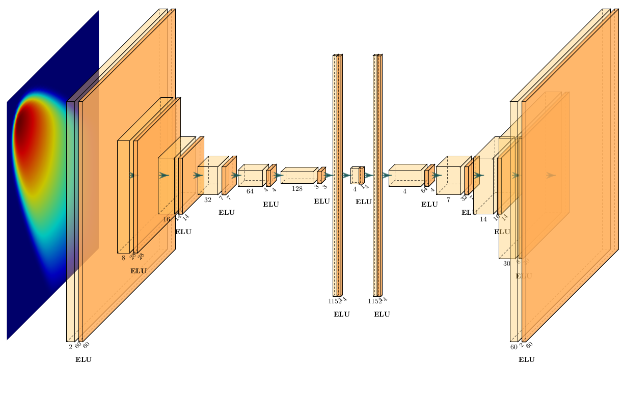
Figure 1: Prototype a convolutional autoencoder architecture employed. The number of layers is the same of the CAE used for the 2d non-linear conservation law test case, but the filter sizes are rescaled for better rendering.

Remark 2 (Regularity).

Regarding the regularity of the CAE, related to the choice of activation functions, it is proved in Theorem 4.2 from  [37] that NM-LSTM and non-linear manifold Galerkin methods are asymptotically equivalent provided that the decoder is twice differentiable. Since we are only employing the NM-LSTM method, our only concern in the choice of activation functions is that the reconstruction error is sufficiently low, so that the accuracy of the whole procedure is not undermined.

For each batch $\{\mathbf{U}_{i}\}_{i=1}^{b}\subset\mathcal{U}_{\text{train}}$, the loss employed is the sum of the reconstruction error, and a regularizing term for the weights:

$$\mathcal{L}(\{\mathbf{U}_{i}^{t_{i}}\}_{i=1}^{b};\Theta)=\frac{1}{b}\sum_{i=1}^{b}\frac{\lVert\mathbf{U}^{t_{i}}_{i}-(\phi\circ\psi)(\mathbf{U}^{t_{i}}_{i})\rVert^{2}_{2}}{\lVert\mathbf{U}^{t_{i}}_{i}\rVert^{2}_{2}}+\lambda_{1}\lVert\Theta\rVert^{2}_{2},$$ (12)

where $\Theta$ represents the weights of the convolutional autoencoder. The choice of the relative mean squared reconstruction error is important when, varying the parameter $\{\bm{\mu}_{i}\}_{i=1}^{N_{\text{train}}}$, the snapshots $\{\mathbf{U}_{i}\}_{i=1}^{N_{\text{train}}}$ have different orders of magnitude: for example this is the case of flows propagating from a local source on the whole domain with a constant zero state as initial condition.

The training is performed with Adam stochastic optimization method [34]. After the training the whole evolution of the dynamics is carried out with a non-linear optimization algorithm minimizing the residual on the latent domain, as described in section 3. For each new parametric instance and associated initial state $\mathbf{U}_{0}\in X_{h}$, the latent initial condition is found with a single forward of the encoder $z_{0}=\psi(\mathbf{U}_{0})$ after centering and normalizing $\mathbf{U}_{0}$. Then, for each time instant $t$, the decoder

$$\phi(z(t))=\mathbf{U}(t)\in(\phi\circ\psi)(X_{h})\subset\mathbb{R}^{d},$$ (13)

is used as parametrization of an approximate solution manifold as will be explained in section 3, including in $\phi$ the renormalization of the output.

Remark 3 (Initial condition).

With respect to the initial implementation of Carlberg et al [37] our approach for the definition of the latent parametrization of the solution manifold is different in the management of the initial condition. Instead of using directly the decoder $\phi$, they define the map from the latent to the state space $f:\mathbb{R}^{r}\rightarrow\mathbb{R}^{d}$, including the renormalizations in the $\phi$ map for brevity, as

$$f(z)=\phi(z)+\mathbf{U}_{0}(\mu)-\phi(\psi(\mathbf{0})),\quad\text{s.t.}\ f(\psi(\mathbf{0}))=\mathbf{U}_{0}(\mu),$$ (14)

so that the reconstruction is exact at the initial parametric time instances. So, supposing that the initial condition is parametrically dependent, all initial conditions coincide to $\psi(\mathbf{0})$ in the latent space, and the decoder has to learn variations from the initial latent condition. We prefer instead to split the initial conditions in the latent space in order to aid the non-linear optimization algorithm, and leave to the training of the CAE the accurate approximation of the initial condition. This splitting of the initial conditions can be seen in Figure 6 and 13. The additional cost of our implementation is the forward of the initial parametric condition through the encoder as first step.

Remark 4 (Inductive biases).

Imposing inductive biases to increase the convergence speed of a deep learning model to the desired solution has always been a winning strategy in machine learning. This is translated in the context of physical models with the possibility to include, among others, the following inductive biases: first principles (conservation laws [36], equations governing the physical phenomenon), geometrical simmetries (group invariant filters [50, 21]), numerical schemes/residuals (discrete residuals, latent time advancement with Runge Kutta schemes), latent regularity (minimize the curvature of latent trajectories), latent dynamics (linear or quadratic latent dynamics [28]). As inductive bias, we will impose the positivity of the state variables that are known to be positive throughout their trajectory with a final ReLU activation.

3 Evolution of the latent dynamics with NM-LSPG-ROC

The non-linear manifold method introduced by Carlberg et al [37] does not perform a complete dimension reduction since at each time step the decoder reconstruct the state from the latent coordinates to the whole domain, still depending on the number of degrees of freedom of the FOM. We revisit the non-linear manifold least-squares Petrov-Galerkin method (NM-LSPG) with small modifications and introduce two novel hyper-reduction procedures: one combines teacher-student training of a compressed decoder with the reduced over-collocation method (NM-LSPG-ROC-TS), the other implements only the hyper-reduction of the residual with reduced over-collocation (NM-LSPG-ROC).

3.1 Non-linear manifold least-squares Petrov-Galerkin

We assume that the numerical method of preference discretizes the system 1 in space and in time with an implicit scheme, $G_{h,\delta t}:\mathcal{P}\times X_{h}\times X_{h}^{|I_{t}|}\rightarrow X_{h}$

$$G_{h,\delta t}(\bm{\mu},\mathbf{U}_{h}^{t},\{\mathbf{U}_{h}^{s}\}_{s\in I_{t}})=\mathbf{0},$$ (15)

where $h,\ \delta t$ are the spatial and temporal discretization steps chosen, $X_{h}\subset\mathbb{R}^{d}$ is the state discretization space ($d$ is the number of degrees of freedom), and $I_{t}$ is the set of past state indexes employed in the temporal numerical scheme to solve for $\mathbf{U}^{t}_{h}$. We remark that the numerical discretization employed can differ from the one used to solve for the full-order training snapshots. The method is thus equations-based rather than fully intrusive. This will be the case for the 2d shallow water equations model in Subsection 4.2.

For each discrete time instant $t$ the following non-linear least-squares problem is solved for the latent state $\mathbf{z}^{t}\in Z$, with the Levenberg-Marquardt algorithm [49]

$$\mathbf{z}^{t}=\operatorname*{\arg\!\min}_{\mathbf{z}\in\mathbb{R}^{r}}\ \lVert G_{h,\delta t}(\bm{\mu},\phi(\mathbf{z}),\{\phi(\mathbf{z}^{s})\}_{s\in I_{t}})\rVert^{2}_{X_{h}}.$$ (16)

That is for each time instant the following intermediate solutions $\{\mathbf{z}^{t,k}\}_{k\in\{0,\dots,N(t)\}},\ \mathbf{z}^{t,0}=\mathbf{z}^{t-1,N(t-1)}$ of the linear system in $\mathbb{R}^{r}$ are computed,

$$\left((dG^{t,k-1}d\phi^{t,k-1})^{T}dG^{t,k-1}d\phi^{t,k-1}+\lambda\ I_{d}\right)\delta\mathbf{z}^{t,k}=-(dG^{t,k-1}d\phi^{t,k-1})^{T}G^{t,k},$$ (17)

$$\mathbf{z}^{t,k}=\mathbf{z}^{t,k-1}+\alpha^{k}\ \delta\mathbf{z}^{t,k},$$ (18)

where $d\phi^{t,k-1}=d\phi(\mathbf{z}^{t,k-1})\in\mathbb{R}^{d\times r}$ and $dG^{t,k-1}=dG_{h,\delta t}(\bm{\mu},\phi(\mathbf{z}^{t,k-1}),\{\phi(\mathbf{z}^{s})\}_{s\in I_{t}})\in\mathbb{R}^{d\times d}$ are the Jacobian matrices of the embedding map $\phi$ and of the residual $dG_{h,\delta t}$ respectively, $\lambda$ is a factor that evolves during the non-linear optimization and balances between a Gauss-Newton and a steepest descent method, and finally $\alpha^{k}$ is a parameter tuned with a line search method. In the implementation in Eigen [30], $\lambda\ I_{d}$ is scaled with respect to the diagonal elements of $(dG^{t,k-1}d\phi^{t,k-1})^{T}dG^{t,k-1}d\phi^{t,k-1}$. All the tolerances for convergence are set to machine precision, and the maximum number of residual evaluations is set to $7$ unless explicitly stated differently in the numerical results section 4.

Remark 5 (Least-squares Petrov-Galerkin).

The method is called manifold LSPG because it refers to the LSPG method usually applied when the manifold is linear. It consists in multiplying the residual to the left with a different matrix $\Psi$ with respect to the linear embedding $\Phi$ of the reduced coordinates into the state space,

$$\Psi^{T}G_{h,\delta t}(\bm{\mu},\Phi\mathbf{z})=0,$$ (19)

where, $\Phi\in\mathbb{R}^{d\times r}$ is the basis of the linear reduced manifold contained in $X_{h}\subset\mathbb{R}^{d}$, $\mathbf{z}\in\mathbb{R}^{r}$, and $\Psi$ is to be defined: the left subspace $\Psi\in\mathbb{R}^{d\times r}$ is used to enforce the orthogonality of the non-linear residual to a left subspace $\mathcal{L}\subset\mathbb{R}^{d}$. Applying Newton’s method because of the nonlinearities, the problem is translated into the iterations for $k=1,\dots,K$:

$$\Psi^{T}dG\Phi\ \delta\mathbf{z}^{k}=-\Psi^{T}G^{k},$$ (20)

$$\mathbf{z}^{k}=\mathbf{z}^{k-1}+\alpha^{k}\ \delta\mathbf{z}^{k}.$$ (21)

The step length $\alpha^{k}$ is computed after a line search along the direction $p^{k}$. Usually $\Phi$ is chosen from a POD basis of the state variable $\mathbf{z}\in X_{h}$. For the left subspace, that imposes orthogonality constraints, different choices can be applied. In general, given the system

$$dG\Phi\ \delta\mathbf{z}^{k}=-G^{k},$$ (22)

the least squares solution is the one orthogonal to the range of $dG\Phi$. In the case of $dG$ symmetric positive definite we have that $\Psi\subset<dG\Phi>=<\Phi>$ i.e. $\Psi=\Phi$ and the method is called Galerkin projection, but in general if this is not true then the optimal left subspace remains $\Psi=dG\Phi$. For examples where the Galerkin projection is not optimal see [11], section 3.4 Numerical comparison of left subspaces. This is often the case for advection-dominated discretized systems of PDEs: in these cases LSPG is preferred to Galerkin projection.

Remark 6 (Manifold Galerkin).

The manifold Galerkin method proposed in [37] assumes that the columns of the Jacobian of the decoder are good approximations of the state velocity space: if a spatial discretization is applied and the residual has the form $\mathcal{G}_{h}(\bm{\mu},\mathbf{U})=\dot{\mathbf{U}}-\mathbf{f}(\bm{\mu},\mathbf{U})$, where $\mathbf{f}$ is a generic, possibly non-linear, vector field, then

$$\dot{\mathbf{z}}=\operatorname*{\arg\!\min}_{\mathbf{v}\in\mathbb{R}^{r}}\lVert d\phi(\mathbf{z})\mathbf{v}-\mathbf{f}(\bm{\mu},\phi(\mathbf{z}))\rVert^{2},$$ (23)

is solved for the latent state velocity, under the hypothesis that $d\phi(\mathbf{z})$ has full-rank and $d\phi$ is a good approximation of the full-order state velocity even if the autoencoder is trained only on the values of the state for different times and parameters, without considering its velocty. If $\phi$ is linear, we obtain the Galerkin method presented in the remark 5, after having applied a temporal discretization scheme and multplied the resulting equation to the left with $d\phi(\mathbf{z})=\Phi$ as is the case for linear Galerkin projection: the discretize-then-project and project-then-discretize approaches are equivalent in this case [37].

The LSPG performs better as shown in [37], even if they are asymptotically equivalent also in the case of a non-linear manifold, provided $\phi$ is twice differentiable. So we have chosen to employ only the NM-LSPG method and do not compare it with the non-linear manifold Galerkin (NM-G) method.

For the numerical tests we have performed, the numerical approximation of the Jacobian of the residual $G_{h,\delta t}(\bm{\mu},\phi(\mathbf{z}),\{\phi(\mathbf{z}^{s})\}_{s\in I_{t}})$ is accurate enough. So in the implementation, at each iteration step the Jacobian of the residual with respect to the latent variable, that is $dG^{t,k-1}d\phi^{t,k-1}$ of equation 17, is approximated with finite differences. The step size is taken sufficiently lower than the distance between consecutive latent states.

3.2 Reduced over-collocation method

At the point of equation 17, the model still depends on the number of degrees of freedom of the full-order model $d$, since at each time step and optimization step the latent reduced variable $\mathbf{z}\in\mathbb{R}^{r}$ is forwarded to the reconstructed state $\mathbf{U}_{h}=\phi(\mathbf{z})\in\mathbb{R}^{d}$. A possible solution is represented by the reduced over-collocation method [15], for which the least squares problem 16 is solved only on a limited number of points $r<r_{h}<<d$,

$$\mathbf{z}^{t}=\operatorname*{\arg\!\min}_{\mathbf{z}\in\mathbb{R}^{r}}\ \lVert P_{r_{h}}G_{h,\delta t}(\bm{\mu},\phi(\mathbf{z}),\{\phi(\mathbf{z}^{s})\}_{s\in I_{t}})\rVert^{2}_{\mathbb{R}^{r_{h}}},$$ (24)

where $P_{r_{h}}$ is the projection onto $r_{h}$ standard basis elements in $\mathbb{R}^{d}$ associated to the over-collocation nodes or magic points and selected as described later. Afterwards the Levenberg-Marquardt algorithm is applied as described in the previous section, to solve the least squares problem  24.

At this point we make the assumption that the method used to discretize the model has a local formulation so that each discrete differential operator can be restricted to the nodes/magic points of the hyper-reduction and consequently, the least-squares problem 24 reduces to

$$\mathbf{z}^{t} =\operatorname*{\arg\!\min}_{\mathbf{z}\in\mathbb{R}^{r}}\ \lVert P_{r_{h}}G_{h,\delta t}(\bm{\mu},P_{r_{h}}(\phi(\mathbf{z})),\{P_{r_{h}}(\phi(\mathbf{z}^{s}))\}_{s\in I_{t}})\rVert^{2}_{\mathbb{R}^{r_{h}}},$$ (25)

$$=\operatorname*{\arg\!\min}_{\mathbf{z}\in\mathbb{R}^{r}}\ \lVert\tilde{G}_{h,\delta t}(\bm{\mu},\tilde{\phi}(\mathbf{z}),\{\tilde{\phi}(\mathbf{z}^{s})\}_{s\in I_{t}})\rVert^{2}_{\mathbb{R}^{r_{h}}},$$ (26)

where the projected residual $\tilde{G}$ is introduced and the compressed decoder $\tilde{\phi}$ is defined to substitute $P_{r_{h}}\circ\phi$ with another embedding from the latent space to the hyper-reduced space in $\mathbb{R}^{r_{h}}$, such that the whole structure of the decoder is reduced as described in subsection 3.4 to further decrease the computational cost.

The Levenberg-Marquardt method is applied also to the hyper-reduced system

$$\left((d\tilde{G}^{t,k-1}d\tilde{\phi}^{t,k-1})^{T}d\tilde{G}^{t,k-1}d\tilde{\phi}^{t,k-1}+\lambda\ I_{d}\right)\delta\mathbf{z}^{t,k}=-(d\tilde{G}^{t,k-1}d\tilde{\phi}^{t,k-1})^{T}\tilde{G}^{t,k},$$ (27)

$$\mathbf{z}^{t,k}=\mathbf{z}^{t,k-1}+\alpha^{k}\ \delta\mathbf{z}^{t,k},$$ (28)

and as for the manifold LSPG method, the Jacobian matrix $d\tilde{G}^{t,k-1}d\tilde{\phi}^{t,k-1}$ is numerically approximated at each optimization step in the implementations.

Remark 7 (Submesh needed to define the hyper-reduced differential operators).

To compute $\tilde{G}_{h,\delta t}$ in the nodes/magic points of the reduced over-collocation method, some adjacent degrees of freedom are needed by the discrete differential operators involved. So, actually, at each time step not only the values of the state variables at the magic points are needed, but also at the adjacent degrees of freedom in the mesh with possible overlappings. We represent the restriction to this submesh of magic points and adjacent degrees of freedom with the projector $P^{s}_{r_{h}}\in\mathbb{R}^{s_{h}\times d}$, where $s_{h}$ is the number of degrees of freedom of the submesh. Equation 26 becomes

$$\mathbf{z}^{t}=\operatorname*{\arg\!\min}_{\mathbf{z}\in\mathbb{R}^{r}}\ \lVert P_{r_{h}}G_{h,\delta t}(\bm{\mu},P^{s}_{r_{h}}(\phi(\mathbf{z})),\{P^{s}_{r_{h}}(\phi(\mathbf{z}^{s}))\}_{s\in I_{t}})\rVert^{2}_{\mathbb{R}^{r_{h}}}.$$ (29)

The stencil around each magic point to consider depends on the type of numerical scheme. Since we are using the finite volume method we have to consider the degrees of freedom of the adjacent cells. For example, for cartesian grids, the schemes chosen for the 2d non-linear conservation law have a stencil of $1$ layer of adjacent cells, $4$ additional nodes in total for a cell of the interior of the mesh. The 2d shallow water equations case requires a stencil of $2$ layers instead, $12$ additional nodes in total for a cell of the interior of the mesh. The two cases are shown in Figure 2.

Figure 2: Left: 100 magic points of the 2d non-linear conservation law test case. Right: 100 magic points of the 2d shallow water test case. The magic points are represented in red, the stencils of the cells and associated degrees of freedom needed for the evaluation of the discrete differential operators are in light-blue. The discarded nodes in the evolution of the dynamics with NM-LSPG-ROC are in blue. The stencil is made by $1$ layer of cells in the NCL case and $2$ layers in the SW case.

3.3 Over-collocation nodes selection

The nodes/magic points of the over-collocation hyper-reduction method should be defined such that

$$P_{r_{h}}=\operatorname*{\arg\!\min}_{P^{T}P\in\mathcal{S}}\ \max_{(\mathbf{z}^{t},\{\mathbf{z}^{s}\}_{s\in I_{t}})\in\mathcal{T}}\ \lVert G_{h,\delta t}(\bm{\mu},(\phi(\mathbf{z})),\{(\phi(\mathbf{z}^{s}))\}_{s\in I_{t}})-P^{T}PG_{h,\delta t}(\bm{\mu},P(\phi(\mathbf{z}^{t})),\{P(\phi(\mathbf{z}^{s}))\}_{s\in I_{t}})\rVert^{2}_{\mathbb{R}^{r_{h}}}$$ (30)

where $\mathcal{S}=\{P\in\mathbb{R}^{r_{h}\times d}|P=(\mathbf{e}_{i_{1}}|\dots|\mathbf{e}_{i_{r_{h}}})^{T}\}$ is the space of projectors onto $r_{h}$ coordinates associated to the standard basis $\{\mathbf{e}_{i}\}_{i\in\{1,\dots,d\}}$ of $\mathbb{R}^{d}$ and $\mathcal{T}$ is the space of discrete solution trajectories varying with respect to $\bm{\mu}$ and the intermediate optimization steps

$$\mathcal{T} =\{(\bm{\mu},t,k,\mathbf{z}^{t,k},\{\mathbf{z}^{s,k}\}_{s\in I_{t}})\in\mathcal{P}\times V_{h,\bm{\mu}}\times V_{h,\bm{\mu},t}\times\mathbb{R}^{d}\times\mathbb{R}^{d\times|I_{t}|}|,$$

$$\left((dG^{t,k-1}d\phi^{t,k-1})^{T}dG^{t,k-1}d\phi^{t,k-1}+\lambda\ I_{d}\right)\delta\mathbf{z}^{t,k}=-(dG^{t,k-1}d\phi^{t,k-1})^{T}G^{t,k}\},$$

where $V_{h,\bm{\mu}}$ is the discrete space of time instants, possibly depending on $h$ and the paremter $\bm{\mu}$, and $V_{h,\bm{\mu},t}$ is the discrete space of optimization steps at time $t$. Essentially we want that the nodes/magic points approximate the residuals among all time steps, optimization steps and parameter instances.

There are many possible algorithms to solve Equation 30 for $P_{r_{h}}$. Usually they are not optimal and compromise between computational cost and accuracy, depending on the problem at hand. Among others, these algorithms are part of the hyper-reduction methods such as empirical interpolation method [5], discrete empirical interpolation method [14], Gauss-Newton tensor approximation (GNAT) [13], space-time GNAT [16] and solution-based non-linear subspace GNAT [17](SNS-GNAT).

In particular, if $\mathcal{G}_{h}(\bm{\mu},\mathbf{U})=\dot{\mathbf{U}}-\mathbf{f}(\bm{\mu},\mathbf{U})$, then, following some considerations that justify SNS-GNAT [17], the training modes employed to find the nodes/magic points of the over-collocation method are represented by the state snapshots instead of the residual fields. We could in principle use the reduced fields $\phi(\mathbf{z})$ but in practice, for the test case we considered, the full-order state snapshots were enough, without even saving the intermediate optimization states.

The procedure is applied at the same time for all the components of the state field $\mathbf{U}\in X_{h}$ and follows a greedy approach. We remark that the spatial discretization must not vary, so that the degrees of freedom correspond to the same spatial and physical quantity over time and for every parameter instance. Some approaches tackle also geometry deformations, but keeping the same number of degrees of freedom in a reference system [52].

The algorithm 1 is an adaptation of GNAT from Algorithm 3 in [12] to the simpler case in which the Jacobian matrix is not considered in the hyper-reduction (since in the LM method the Jacobian matrix is approximated with finite differences from the residual, see equation 28). Also with respect to Algorithm 3 in [12], the new node/magic point at line 16 in Algorithm 1 is found without computing also the reconstruction error of the degrees of freedom associated to its stencil.

1

input : training state fields $\mathcal{U}_{\text{train}}:=\{\mathbf{U}_{\bm{\mu},t}\}_{\mu\in\mathcal{P}_{\text{train}},\ t\in V_{\bm{\mu},h}}$, such that $|\mathcal{U}_{\text{train}}|=n_{\text{train}}$,

$r_{\text{init}}$ nodes/magic points at the boundaries and forcefully added,

number of nodes/magic points $r_{h}$,

$N_{\text{modes}}$ number of training modes extracted to compute nodes/magic points.

output :  $r_{h}$ nodes/magic points used to define $P_{r_{h}}$.

2

3Extract $N_{\text{modes}}$ modes $\{\phi^{i}_{\mathbf{U}}\}_{i\in\{1,\dots,N_{\text{modes}}\}}$ from the SVD of $\mathcal{U}_{\text{train}}$.

4 Compute the additional number of nodes to sample $n_{a}=r_{h}-r_{\text{init}}$.

5 Initialize counter for the number of working basis vectors used: $n_{b}=0$.

6 Set the number of greedy iterations to perform: $n_{it}=\min{n_{c},n_{a}}$.

7 Compute the minimum number of working basis vectors per iteration: $n_{\text{ci},\text{min}}=\text{floor}(n_{c}/n_{i}t)$.

8 Compute the minimum number of sample nodes to add per iteration: $n_{\text{ai},\text{min}}=\text{floor}(n_{a}/n_{c})$.

9 for $i=1,\dots,n_{it}$ do greedy iteration loop

10      Compute the number of workin basis vectors for this iteration: $n_{ci}=n_{\text{ci},\text{min}}$; If $i\leq n_{c},\ \text{mod}\ n_{it}$ then $n_{ci}=n_{ci}+1$.

11       Compute the number of samples nodes to add during this iteration: $n_{ai}=n_{\text{ci},\text{min}}$; If $i\leq n_{a},\ \text{mod}\ n_{c}$ then $n_{ai}=n_{ai}+1$.

12       if $i=1$ then

13            $\left[\mathbf{U}^{1}\cdots\mathbf{U}^{{n}_{ci}}\right]=\left[\phi^{1}_{\mathbf{U}}\cdots\phi^{n_{ci}}_{\mathbf{U}}\right]$,

14             build the intermediate projection $P$ from the $r_{\text{init}}$ initial nodes/magic points.

15      else

16            for $q=1,\dots,n_{ci}$ do basis vector loop

17                  $\mathbf{U}^{q}=\phi^{n_{q}+q}_{\mathbf{U}}-\left[\phi^{1}_{\mathbf{U}}\cdots\phi^{n_{b}}_{\mathbf{U}}\right]\alpha$, with $\alpha=\operatorname*{\arg\!\min}_{\gamma\in\mathbb{R}^{n_{b}}}\lVert\left[P\phi^{1}_{\mathbf{U}}\cdots P\phi^{n_{b}}_{\mathbf{U}}\right]\gamma-P\phi^{n_{b}+q}_{\mathbf{U}}\rVert_{2}$

18            

19      for $j=1,\dots,n_{ai}$ do sample node loop

20            Find the node/magic point $n$ that maximize the state reconstruction error among the nodes not selected yet: $n=\operatorname*{\arg\!\max}\sum_{q=1}^{n_{ci}}(U^{q})^{2}$.

21             Update $P$ with the newly found node/magic point.

22      $n_{b}=n_{b}+n_{ci}$

Algorithm 1 Greedy nodes/magic points evaluation for ROC method.

Remark 8 (Comparison beetween GNAT and reduced over-collocation).

We must say that the GNAT method, employed for the implementation of NM-LSPG with shallow masked autoencoders in [33], is a generalization of the reduced over-collocation method. In some cases though, they may perform similarly. For $P\in\mathcal{S}$, let us define

$$\mathbf{r}=r_{t,\bm{\mu},k}=G_{h,\delta t}(\bm{\mu},P(\phi(\mathbf{z}^{t,k})),\{P(\phi(\mathbf{z}^{s,k-1}))\}_{s\in I}),\ \forall(t,k,\bm{\mu})\in V_{h,\bm{\mu}}\times V_{h,\bm{\mu},t}\times\mathcal{P},$$ (31)

and the GNAT projection operator $\mathbb{P}=\Phi(P\Phi)^{\dagger}P$, where $\Phi$ is the matrix where the columns correspond to a chosen basis (it could be the FOM residual snapshots, ROM residual snapshots, ROM jacobian and residual snapshots, see [13]). In particular, if $\Phi=P_{r_{h}}^{T}=P^{T}$ we have that

$$\mathbb{P}=\Phi(P_{r_{h}}\Phi)^{\dagger}P_{r_{h}}=\Phi(P_{r_{h}}\Phi)^{-1}P_{r_{h}}=P_{r_{h}}^{T}(P_{r_{h}}P_{r_{h}}^{T})^{-1}P_{r_{h}}=P_{r_{h}}^{T}P_{r_{h}},$$ (32)

that is the reduced over-collocation projection in the chosen nodes/magic points and extended to $0$ in the remaining degrees of freedom. In this sense, the GNAT method includes the reduced over-collocation one.

However, for the class of problems we are considering, the GNAT method suffers from the slow decaying KnW. We have the inequalities

$$d_{n}^{2}(\{r_{t,\bm{\mu},k}\}_{t,\bm{\mu},k}) =\inf_{\text{dim}V_{n}=n}\max_{t,\bm{\mu},k}\lVert\mathbf{r}-V_{n}V_{n}^{T}\mathbf{r}\rVert^{2}_{2}\leq\inf_{\text{dim}V_{n}=n}\max_{t,\bm{\mu},k}\lVert\mathbf{r}-V_{n}V_{n}^{T}\mathbf{r}\rVert^{2}_{2}+\lVert V_{n}V_{n}^{T}\mathbf{r}-\mathbb{P}\mathbf{r}\rVert^{2}_{2}$$

$$=\inf_{\text{dim}V_{n}=n}\max_{t,\bm{\mu},k}\lVert\mathbf{r}-\mathbb{P}\mathbf{r}\rVert^{2}_{2}=\inf_{\text{dim}V_{n}=n}\max_{t,\bm{\mu},k}\lVert(I-\mathbb{P})(I-V_{n}V_{n}^{T})\mathbf{r}\rVert^{2}_{2}$$

$$\leq\inf_{\text{dim}V_{n}=n}\max_{t,\bm{\mu},k}\lVert(I-\mathbb{P})\rVert_{2}^{2}\lVert(I-V_{n}V_{n}^{T})\mathbf{r}\rVert^{2}_{2}=\inf_{\text{dim}V_{n}=n}\max_{t,\bm{\mu},k}\lVert\mathbb{P}\rVert_{2}^{2}\lVert(I-V_{n}V_{n}^{T})\mathbf{r}\rVert^{2}_{2},$$

where $(t,k,\bm{\mu})\in V_{h,\bm{\mu}}\times V_{h,\bm{\mu},t}\times\mathcal{P}$ whenever the maximum is taken. The term $\mathbf{r}-\mathbb{P}\mathbf{r}$ is the GNAT approximation error. The rightmost term is the usual bound on the hyper-reduction error [14], where it was used the fact that $\mathbb{P}=I-\mathbb{P}$. The second equality is valid because $\mathbf{r}-V_{n}V_{n}^{T}\mathbf{r}$ and $V_{n}V_{n}^{T}\mathbf{r}-\mathbb{P}\mathbf{r}$ are orthogonal. The third equality is obtained from the relations

$$\mathbf{r}=(\mathbf{r}-\mathbf{r}_{*})+\mathbf{r}_{*}=\mathbf{w}+\mathbf{r}_{*},\qquad\text{with}\ \mathbf{r}_{*}:=V_{n}V_{n}^{T}\mathbf{r},$$

$$\Rightarrow\quad \mathbf{r}-\mathbb{P}\mathbf{r}=\mathbf{w}+\mathbf{r}_{*}-\mathbb{P}\mathbf{w}-\mathbb{P}\mathbf{r}_{*}=\mathbf{w}-\mathbb{P}\mathbf{w},$$

where the last equality follows from $\mathbb{P}\mathbf{r}_{*}=\mathbf{r}_{*}$. Here we have supposed the nodes/magic points to be independent from $V_{n}$. So in the case of slow decaying Kolmogorov n-width, minimizing the hyper-reduced residual $\mathbb{P}\mathbf{r}\in<V_{n}>\subset\mathbb{R}^{d}$ is less efficient due to the slow convergence in $n$ of the best approximation error $\lVert\mathbf{r}-V_{n}V_{n}^{T}\mathbf{r}\rVert^{2}_{2}$. This is one of the reasons why we employed ROC for the SWE test case; for the NCL test case GNAT and ROC performed similarly.

3.4 Compressed decoder teacher-student training

In order to make the whole methodology independent from the number of degrees of freedom, the decoder has to be substituted with a map $\tilde{\phi}:\mathbb{R}^{R}\rightarrow P_{r_{h}}(X_{h})\subset\mathbb{R}^{r_{h}}$ from the latent space to the space of discrete full-order solutions evaluated only at the submesh containing the magic points and the needed adjacent degrees of freedom. As architecture, we choose a feedforward neural network (FNN) with one hidden layer, but actually the only requirement is that the computational cost is low enough such that not only a theoretical dimension reduction is achieved but also a speed-up is reached.

In the literature, the procedure for the training of the compressed decoder $\tilde{\phi}$ from the decoder $\phi$ is called teacher-student training [27]. In principle, the compressed decoder can be composed from layers inherited by the original decoder, such that the learning process involves only the final new additional layers. In our case, we preferred to train the compressed decoder anew: the latent projections of the training snapshots with the encoder $\psi(\mathcal{U}_{\text{train}})=\{z_{i}\}_{i=1}^{N_{\text{train}}}$ are the inputs and the restriction of the snapshots to the submesh $P^{s}_{r_{h}}(\mathcal{U}_{\text{train}})=\{\tilde{U}_{i}\}_{i=1}^{N_{\text{train}}}$ are the targets, see Equation 29. A schematic representation of the teacher-student training is represented in figure 3. Moreover, to speed-up the offline tage, we use the training FOM snapshots restricted to the magic points as training outputs for the teacher-student training, while usually the reconstructed snapshots from the CAE -that would additionaly need to be computed- are employed.

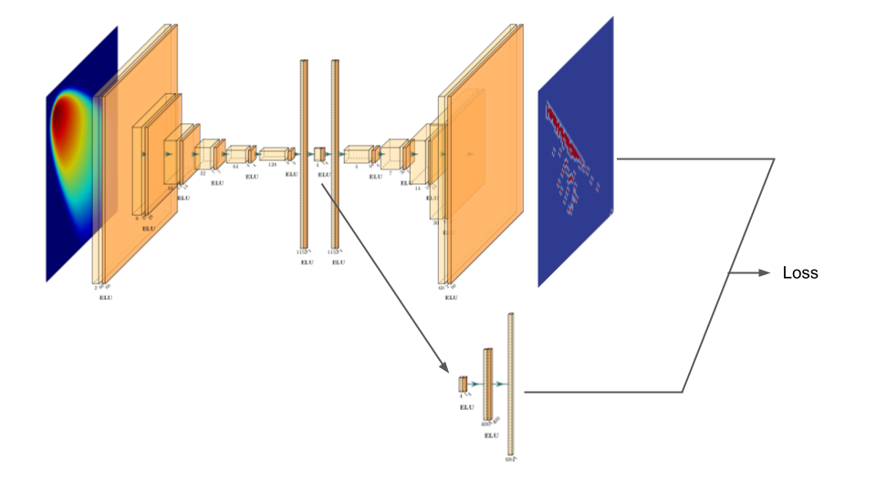
Figure 3: Teacher-student training of the compressed decoder for the 2d non-linear conservation law test case. The magic points, which the snapshots are restricted to, are shown in red over the domain.

Again, for the training, we use a relative mean square loss with an additional regularizing term

$$\mathcal{L}(\{z_{i}\}_{i=1}^{b};\tilde{\Theta})=\frac{1}{b}\sum_{i=1}^{b}\frac{\lVert\tilde{U}_{i}-\tilde{\phi}(z_{i})\rVert^{2}_{2}}{\lVert\tilde{U}_{i}\rVert^{2}_{2}}+\lambda_{1}\lVert\tilde{\Theta}\rVert^{2}_{2},$$ (33)

where $\tilde{\Theta}$ are the weights of the compressed decoder.

Remark 9 (Jacobian evaluation in Levenberg-Marquardt algorithm).

The main reason why finite differences approximations of Jacobians are implemented in the NM-LSPG case, as explained at the end of subsection 3.1, is that the computational cost of evaluating the Jacobian of the full decoder is too high. In principle Jacobian evaluations of the compressed decoder are cheaper and could be employed, instead of relying again on finite differences approximations.

Remark 10 (Shallow masked autoencoders).

We are motivated to write this article to extend the results in [33] to a generic architecture composed by neural networks. They performed the hyper-reduction of the non-linear manifold method [37] with a shallow masked autoencoder, so that correctly masking the weights matrices of the decoder, its outputs correspond only to the submesh needed by the GNAT method, thus eliminating the dependence on the FOM’s degrees of freedom. We want to reproduce, in some sense, this approach for an arbitrary autoencoder architecture, in this case a CAE, in order to takle with the latest architectures developed in the literature the problem of solution manifold approximability: we think this is a major concer when trying to apply non-linear MOR to real applications. In fact, as will be clear in the numerical results section 4, the reconstruction error of the autoencoder bounds from below the prediction error of our newly developed ROMs.

It can be seen that the new model order reduction is composed of two distinct procedures to achieve the independency on the number of degrees of freedom: first the residual from NM-LSPG in Equation 16 is hyper-reduced with ROC in Equation 24 and secondly the CAE’s decoder is compressed with teacher-student training. In principle, we could substitute the use of the compressed decoder with the restriction of the final layer of the CAE’s decoder into the magic points, while keeping the hyper-reduction with ROC of the residual. In this case, the whole methodology would still be dependent on the total number of degrees of freedom, but in practice a CAE’s decoder forward is relatively cheap compared to the evaluation of the full residual. So, the hyper-reduction performed with ROC or GNAT only at the equations/residuals level, is already beneficial to reduce the computational cost. We will compare this variant of the NM-LSPG-ROC method with the one that employs the compressed decoder, also to verify the consistency of the teacher-student training that is omitted in the first case.

In the numerical results section 4 we will adopt the acronym NM-LSPG-ROC-TS or NM-LSPG-GNAT-TS for the method that employs the compressed decoder and NM-LSPG-ROC or NM-LSPG-GNAT for the method that performs the hyper-reduction only at the equations/residuals level.

4 Numerical results

We test the new methodology on two benchmarks with a relatively slow KnW: the first model is governed by a non-linear conservation law 4.1 the second by the shallow water equations 4.2. Both are parametric, non-linear and time-dependent, and the only other (non-temporal) parameter is a multiplicative constant of the initial conidition. The mesh employed is the same: a $60\times 60$ structured orthogonal grid.

All the CFD simulations are obtained by the use of an in-house open source library ITHACA-FV (In real Time Highly Advanced Computational Applications for Finite Volumes) [51], developed in a finite volume environment based on the open-source library OpenFOAM [1]. Regarding the implementation of the convolutional autoencoders and compressed decoders (CAE) we used LibTorch, PyTorch C++ frontend, while for the training of the long-short term memory network (LSTM) we used PyTorch [44]. All the CFD simulations were performed on a Intel(R) Core(TM) i7-8750H CPU with 2.20GHz and all the neural networks trainings on a GeForce GTX 1060 GPU. Further reductions in the computational costs could be achieved exploiting the parallel implementation of the training procedures in PyTorch. The details of the architectures of the neural networks that will be employed are reported in the Appendix A.

The following notations are introduced: $N^{\mu}_{\text{train}},\ N^{\mu}_{\text{test}}$ are the numbers of train and test parameters, respectively; $N^{t}_{\text{train}},\ N^{t}_{\text{test}}$ are the number of time instances associated to the train and test parameters, respectively. The total number of training and test snapshots is thus $N_{\text{train}}=N^{\mu}_{\text{train}}\cdot N^{t}_{\text{train}}$, and $N_{\text{test}}=N^{\mu}_{\text{test}}\cdot N^{t}_{\text{test}}$, respectively.

The accuracy of the reduced-order models devised is measured with the mean realtive $L^{2}$-error and the maximum relative $L^{2}$-error, where the mean and max are taken with respect to the time scale: since the test cases depend on a non-temporal parameter, for each instance of these parameters a time-series corresponding to the discrete dynamics is associated; the mean and maximum are evaluated w.r.t the elments of these time-series. Let $\{u^{t_{i}}_{\mu}\}_{i=1,\dots N^{t}}$ and $\{U^{t_{i}}_{\mu}\}_{i=1,\dots N^{t}}$ be the predicted and true time-series $N^{t}$ elements long, associated to the train or test parameter $\mu$, the mean relative $L^{2}$-errors and maximum relative $L^{2}$-errors are then defined as

$$\epsilon_{mean}(u_{\mu},U_{\mu})=\frac{1}{N^{t}}\sum_{i=1}^{N^{t}}\frac{\lVert u^{t_{i}}_{\mu}-U^{t_{i}}_{\mu}\rVert_{L^{2}}}{\lVert U^{t_{i}}_{\mu}\rVert_{L^{2}}},\qquad\epsilon_{max}(u_{\mu},U_{\mu})=\max_{i=1,\dots,N^{t}}\frac{\lVert u^{t_{i}}_{\mu}-U^{t_{i}}_{\mu}\rVert_{L^{2}}}{\lVert U^{t_{i}}_{\mu}\rVert_{L^{2}}}.$$ (34)

Remark 11 (Levenberg-Marquardt parameters).

Regarding the Levenberg-Marqurdt non-linear optimization algorithm, we remark that we approximate the Jacobians with forward finite differences, and the optimization process, for each time step, is stopped when the maximum number of residual evaluations is reached. This number is set to $7$, including the evaluations related to the Jacobian computations. When $7$ residual evaluations are not enough for the method to converge, it is explicitly reported.

4.1 Non-linear conservation law (NCL)

We test our procedure for non-linear model order reduction on a 2d non-linear conservation law model (NCL). Two main reasons are behind this choice: the slow Kolmogorov n-width decay of the continuous solution manifold, and the possibility to compare our results with a similar test case realized with an implementation of non-linear manifold based on shallow masked autoencoders and GNAT [33].

The parametrization affects the initial velocity as a scalar multiplicative constant $\mu\in[0.8,2]$:

$$\begin{cases}\partial_{t}\mathbf{u}+\frac{1}{2}\nabla\cdot\left(\mathbf{u}\otimes\mathbf{u}\right)=\nu\Delta\mathbf{u}&(\mathbf{x},t)\in[0,1]^{2}\times[0,2],\\ \mathbf{u}(\mathbf{x},0)=0.8\cdot\mu\cdot\sin(2\pi x)\sin(2\pi y)\chi_{[0,0.5]^{2}}&\mathbf{x}\in[0,1]^{2},\\ \mathbf{u}(\mathbf{x},t)=0&(\mathbf{x},t)\in\partial[0,1]^{2}\times[0,2],\end{cases}$$ (35)

where the viscosity $\nu=0.0001$. We will collect $N^{\mu}_{\text{train}}=12$ equispaced training parameters from the range $\mu\in[0.8,2]$ and $N^{\mu}_{\text{test}}=16$ equispaced test parameters from the range $\mu\in[0.6,2.2]$. The first two and the last two parameters will account for the extrapolation error. The time step is equal to $\Delta t=1\mathrm{e}-3$ seconds, but the training snapshots are collected every $4$ timesteps and the test snapshots every $20$, thus $N^{t}_{\text{train}}=501$, and $N^{t}_{\text{test}}=101$. In the predictive online phase, the dynamics will be evolved with the same timestep $\Delta t=1\mathrm{e}-3$. For easyness of representation, the train parameters are labelled from $1$ to $12$, and the test parameters are labelled from $1$ to $16$.

To have a qualitative view on the range of the solution manifold, we report the initial and final time snapshots for the extremal training parameters of the range $\mu\in[0.8,2]$, in Figure 4.

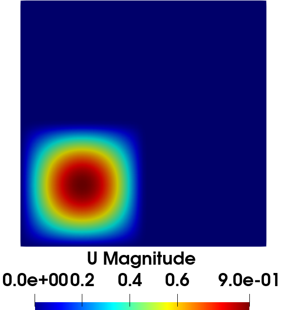
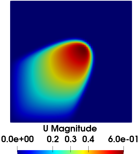
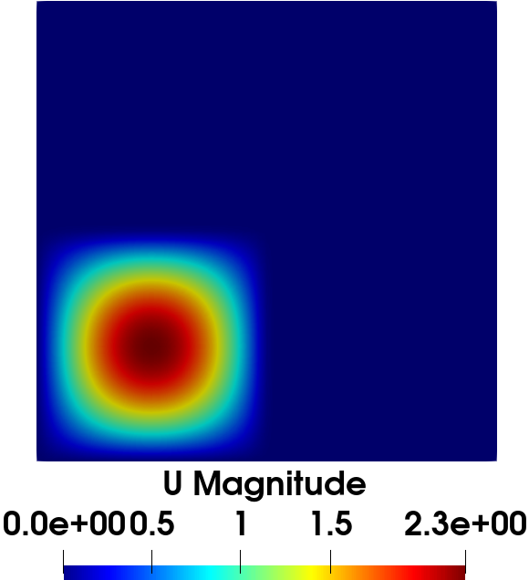
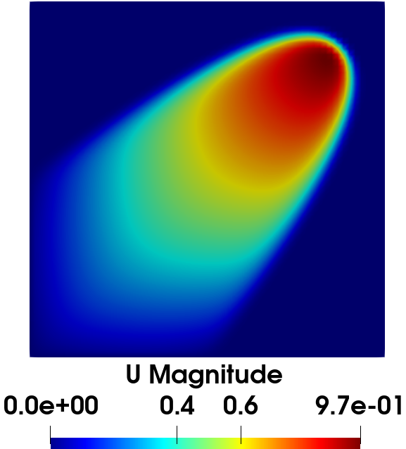
Figure 4: From left to right: FOM solution of equation 35 at $(t,\mu)\in\{(0,0.8),(2,0.8),(0,2),(2,2)\}$.

In this test case the GNAT method performed slightly better than the ROC method for hyper-reduction so we employed the former to obtain the results shown.

4.1.1 Full-order model

We solve the 2d non-linear conservation law for different values of the parameter $\mu$ with OpenFoam [1] open-source software for CFD. We employ the finite volumes method (FVM) in a structured orthogonal grid of $60\times 60$ cells. If we represent with $M$ the mass matrix, with $D$ the diffusive matrix term, and with $C(U^{t-1})$ the advection matrix, then, at every time instant $t$, the discrete equation

$$\frac{M}{\Delta t}U^{t}+C(U^{t-1})U^{t}-\nu DU^{t}=\frac{M}{\Delta t}U^{t-1},$$ (36)

is solved for the state $U^{t}$ with a semi-implicit Euler method. The time step is $1\mathrm{e}-3$, the initial and final time instants are $0$ and $2$ seconds. The linear system is solved with the iterative method BiCGStab preconditioned with DILU, until a tolerance of $1\mathrm{e}{-17}$ on the FVM residual is reached.

The stencil of the numerical scheme at each cell involves the adjacent cells that share an interface ($4$ for an interior cell, $3$ for a boundary cell and $2$ for a corner cell): the value of the state at the interfaces is obtained with the bounded upwind method for the advection term and the surface normal gradient is obtained with central finite differences of two adjacent cell centers. So, in order to implement the reduced over-collocation method, for each node/magic point we have to consider an additional number of maximum $4$ cells, that is $8$ degrees of freedom to keep track of during the evolution of the latent dynamics; of course in practice they may overlap reducing the computational cost furtherly.

The residual of the NM-LPSG methods is evaluated with the same numerical scheme of the FOM. In the SWE test case the FOM and the ROMs employ different numerical schemes 4.2.

4.1.2 Manifold learning

As first step of the procedure the discrete solution manifold is learned through the training of a convolutional autoencoder (CAE) whose specific architecture is reported in Table 7. The CAE is trained with the ADAM [34] stochastic optimization algoritm for $2000$ epochs, halving the learning rate by a factor of $2$ if after $200$ epochs the loss does not decrease. The initial learning rate is $1\mathrm{e}{-3}$, its lower bound is $1\mathrm{e}{-6}$. The number of training snapshots is $N_{\text{train}}=12\times 501=6012$, the batch size $20$. It could be furtherly refined in order the increase the efficiency of the whole procedure.

We choose as latent dimension $4$, $2$ dimensions greater than the number of parameters (the scalar multiplying the initial condition and time). We don’t perform a convergence study of the accuracy with respect to the latent dimension since our focus is on the implementation of the NM-LSPG-ROC and NM-LSPG-ROC-TS model-order reduction methods: we are satisfied as long as the accuracy is relatively high, while the reduced dimension corresponds to an inaccurate linear approximating manifold spanned by the same number of POD modes.

In Figure 5 is shown the reconstruction error of the CAE and its decay with respect to the number of POD modes chosen $[4,10,25,50,100]$. To reach the same accuracy of the CAE with latent dimension $4$, around $50$ POD modes are needed. In order to state that the slow KnW decay problem is overcome by the CAE, the asymptotic convergence of the reconstruction error w.r.t. the latent dimension should be studied as was done for similar problems in [37, 33]. Instead, we will empirically prove that we can devise an hyper-reduced ROM with latent dimension $4$ and accuracy lower than the $2\%$ for the mean relative $L2$-error, a task that would be impossible for a POD based ROM with the same reduced dimension, since the reconstruction error is near $20\%$ for all the test parameters.

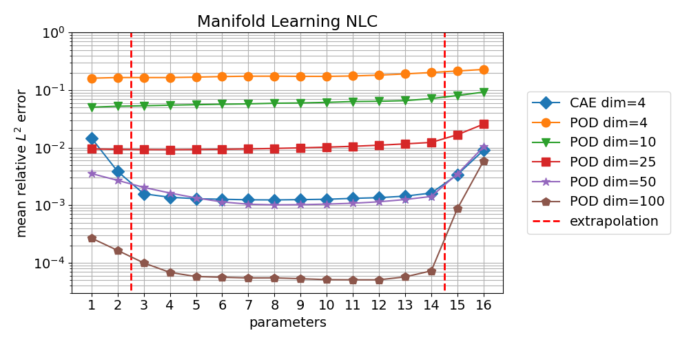
Figure 5: Comparison between the CAE’s and POD’s projection errors of the discrete solution manifold represented by the $N_{\text{train}}=N^{\mu}_{\text{train}}\cdot N^{t}_{\text{train}}=12\cdot 501$ training snapshots. The error is evaluated on the $16$ test parameters, each associated with a time series of $N^{t}_{\text{test}}=101$, for a total of $N_{\text{test}}=N^{\mu}_{\text{test}}\cdot N^{t}_{\text{test}}=16\cdot 101=1616$ test snapshots. The mean is performed over the time scale.

Without imposing any additional inductive bias a part from the regularization term in the loss from Equation 12 and the positiveness of the velocity components, the latent trajectories reported in Figure 6 for the odd parameters of the test set, are qualitatively smooth. An important detail to observe is that the initial conditions are well separated one from another in the latent space, see Remark 3, and that the dynamics is non-linear. It also can be noticed that the $2$ extremal parameters, corresponding to the extrapolation regime and represented in the plot by the two most outer trajectories that enclose the other $6$, have smooth latent dynamics analogously to the others even though the reconstruction error starts degrading, as can be seen from Figure 5.

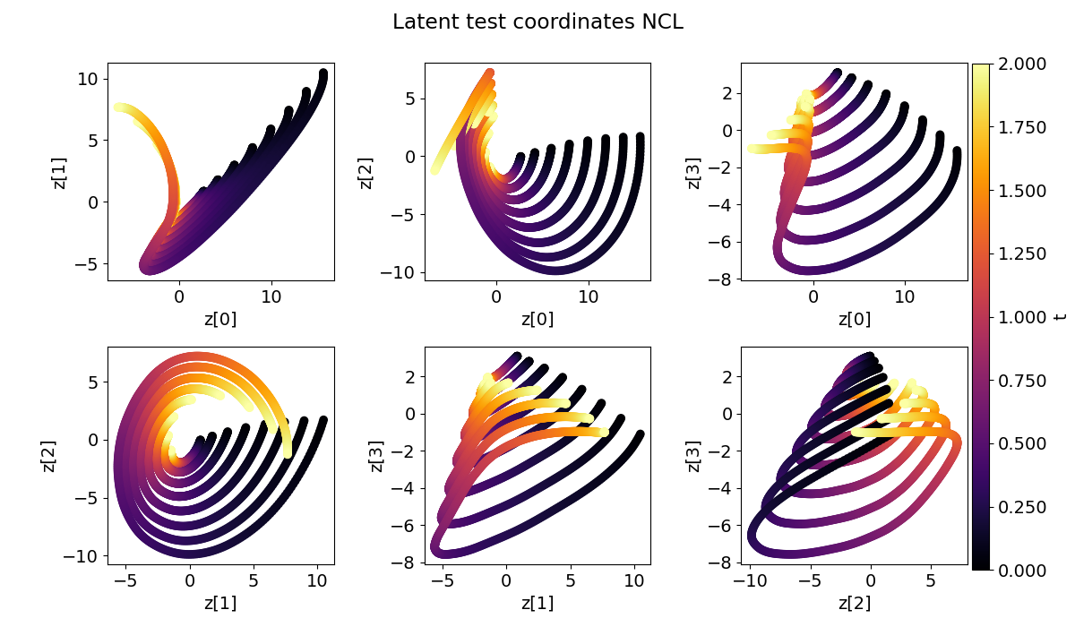
Figure 6: Correlations among the $4$ latent coordinates of the odd parameters of the test set, $8$ in total. They are obtained projecting the test snapshots into the latent space of the CAE with the encoder. The coloring corresponds to the time instants from $0$ to $2$.

4.1.3 Hyper-reduction and teacher-student training

The selection of the magic points is carried out with the greedy Algorithm 1. The FOM snapshots employed correspond to the training parameters $1$ and $12$, but are sampled every $10$ time step instead of every $4$, as for the training snapshots of the CAE.

We perform a convergence study increasing the number of magic points from $50$ to $100$ and $150$. The corresponding submesh sizes, i.e. the number of cells involved in the discretization of the residuals, are reported in the Table 1. The submesh size is bounded above with the total number of the cells in the mesh, that is $3600$.

After the computation of the magic points, the FOM snapshots are restricted to those cells and employed as training outputs of the compressed decoder, as described in Section 3.4. The actual dimension of the outputs is twice the submesh size, since for each cell there are $2$ degrees of freedom corresponding to the velocity components. The inputs are the $4$-dimensional latent coordinates of the encoded FOM training snapshots, for a total of $6012$ training input-output pairs. The architecture of the compressed decoder is a feedforward neural network (FNN) with one hidden layer, whose number of nodes is reported in Table 1, under ’HL size’. The compressed decoders architecture’s specifics are also summarized in Table 7.

Each compressed decoder is trained for $3000$ epochs, with an initial learning rate of $1\mathrm{e}-4$, that halves if the loss from Equation 33 does not decrease after $200$ epochs. The batch size is $20$. The duration of the training is reported in Table 1 under ’TS total epochs’, that stands for Teacher-Student training total epochs, along with the average cost for an epoch, under ’TS avg epoch’. The accuracy of the predictions on the test snapshots restricted to the magic points is assessed in Figure 7.

Table 1: In this table are reported for the NCL test case: the submesh size and the hidden layer (HL) number of nodes of the compressed decoder; the Teacher-Student training (TS) duration in secods (TS total epochs), the Teacher-Student training average epoch duration in seconds (TS avg epoch); the average time step for NM-LSPG-GNAT with compressed decoder (avg GNAT-TS) in milliseconds, and the average time step for NM-LSPG-GNAT with the hyper-reduced residuals but full CAE decoder (avg GNAT-no-TS) in milliseconds. In red, the results are obtained with $13$ maximum residual evaluations of the Levenberg-Marquardt algorithm, instead of the fixed $7$, see Remark 11.

MP	Submesh size	HL size	TS total epochs	TS avg epoch	avg GNAT-TS	avg GNAT-no-TS
50	139	300	1682 s	0.560 s	1.88 ms	4.496 ms
100	246	350	2482 s	0.827 s	4.599 ms	4.499 ms
150	335	400	4245 s	1.415 s	2.318 ms	4.208 ms

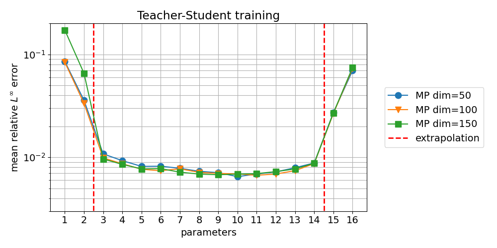
Figure 7: Prediction accuracy on the test snapshots restricted to the magic points. The accuracy is measured with the relative $L^{\infty}$-error averaged over the time trajectories associated to each one of the $N^{\mu}_{\text{test}}=16$ test samples.

The convergence with respect to the number of magic points is shown in Figure 8. Since, especially for the NM-LSPG-GNAT-TS reduced-order model, the relative $L^{2}$-error is not uniform along the time scale, we report both the mean and max relative $L^{2}$-errors over the time series associated to each one of the $16$ test parameters.

From Figure 8 and Table 1 it can be seen that NM-LPSG-GNAT is more accurate than NM-LSPG-GNAT-TS even tough computationally more costly in the online stage. We underline that in the offline stage NM-LSPG-GNAT-TS requries the training of the compressed decoder. However, this could be performed at the same time of the CAE training, see the discussion section 5. The NM-LSPG-GNAT reduced-order model achieves better results also in the extrapolation error, sometimes even lower than the NM-LSPG method: this remains true even when increasing the maximum residual evaluations of the LM algorithm and it may be related to the nonlinearity of the decoder that introduces difficult to interpret correlations of the latent dynamics with the output solutions restricted to the magic points.

All the simulations of NM-LSPG, NM-LSPG-GNAT-TS and NM-LSPG-GNAT methods converge with a maximum of $7$ residual evaluations of the LM algorithm, for all magic points reported, that is $50$, $100$, and $150$ and for all the $16$ test parameters. However, $3$ test parameters could not converge for the method NM-LSPG-GNAT-TS with $100$ magic points, so we increased the maximum function evaluations to $13$ for all the test points. The higher computational cost per time step is shown in Table 1. A part from those $3$ test points not converging, the accuracy remains the same for the other $13$ test parameters, so we have chosen to report the results in the case of $13$ residual evaluations for all the $16$ test parameters in Figure 8.

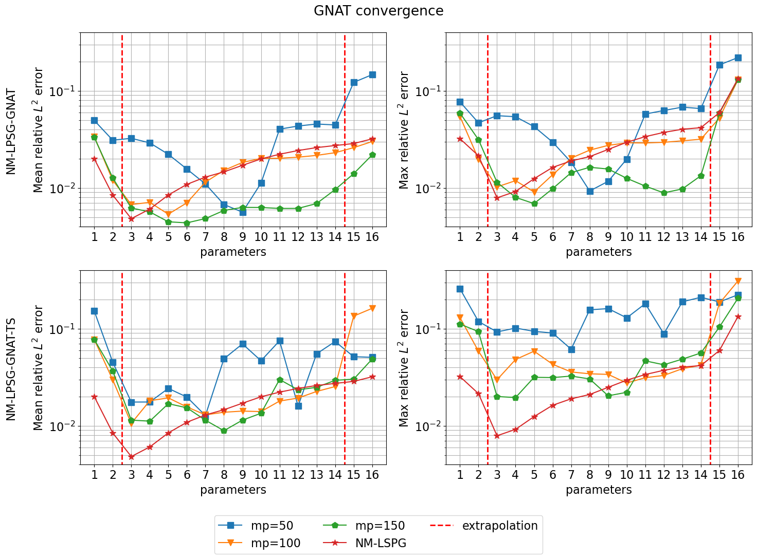
Figure 8: First row: NM-LSPG-GNAT mean and max relative $L^{2}$-error. Second row: NM-LSPG-GNAT-TS mean and max relative $L^{2}$-error. In red also the NM-LSPG accuracy is reported. The mean and max values are evaluated with respect to the time series of intermediate solutions associated to each one of the $N^{\mu}_{\text{test}}=16$ test parameters.

4.1.4 Comparison with data-driven predictions based on a LSTM

To asses the quality of the reduced-order models devised, we compare the accuracy in the training and extrapolation regimes, and the computational cost of the offline and online stages with a purely data-driven ROM in which the solutions manifold is approximated by the same CAE, but the dynamics is evolved in time with a LSTM neural network. The architecture of the LSTM employed is reported in Table 9. The results are summarized in Figure 9, the computational costs in Table 2.

The LSTM is trained for $10000$ epochs with the ADAM stochastic optimization algorithm and an initial learning rate of $0.001$, halved if after $500$ epochs the loss does not decrease. The time series used for the training are the same $N_{\text{train}}=6012$ training snapshots employed for the CAE. We remark that the LSTM cannot approximate the dynamics for an arbitrary time step, but it is fixed, depending on the training time step used, in this case $0.004$ seconds.

The offline stage’s computational cost is determined by the heavy CAE training for both the procedures, see the Discussion section 5 for possible remedies. The LSTM-NN achives a speed-up close to $3$ with respect to the FOM, differently from the NM-LSPG-GNAT and NM-LSPG-GNAT-TS methods. However, since the models are hyper-reduced, increasing the degrees of freedom refining the mesh should increase the computational cost of the FOM and NM-LSPG methods only, with due precautions. The average cost of the evaluation of the dynamics for the LSTM model with a time step of $0.004$ seconds is associated to the label ’avg LSTM-NN full-dynamics’; thanks to vectorization, the dynamics for all the $N^{\mu}_{\text{test}}=16$ parameters is evlauated with a single forward of the LSTM, thus the low computational cost reported.

Table 2: Offline stage: full-order model (FOM) computation of the $N_{\text{train}}=6012$ snapshots (FOM snapshots evaluation), average cost of a single epoch for the training of the CAE with a batch size of $20$ (CAE training single epoch avg), and total cost for $3000$ epochs (CAE training); average epoch’s cost for the LSTM training with a batch size of $100$, and total cost for $10000$ epochs. Online stage: for the FOM, NM-LSPG and LSTM-NN models it is reported the average of a single time step cost over all the $N_{\text{test}}=1616$ test parameters and time series, and the average cost of the full dynamics over the $N^{\mu}_{\text{test}}=16$ test parameters. The LSTM-NN full-dynamics is evaluated with a single forward.

Offline stage	Time
FOM snapshots evaluation	29.04 [s]
CAE training single epoch avg	10.1 [s]
CAE training	20213.3 [s]
LSTM-NN training single epoch avg	0.139 [s]
LSTM-NN training	1365 [s]

Online stage	Time
avg FOM time step	1.210 [ms]
avg FOM full dynamics	2.42 [s]
avg NM-LSPG time step	22.126 [ms]
avg NM-LSPG full-dynamics	133.2 [s]
avg LSTM-NN time step	0.432 [ms]
LSTM-NN full-dynamics	6.982 [ms]

The CAE reconstruction error in blue in Figure 9, lower bounds all the other models’ errors. This is the reason why having a good accuracy of the CAE’s solution manifold approximation is mandatory to build up non-linear manifold methods. In this sense NM-LSPG-ROC-TS and NM-LSPG-GNAT-TS with respect to NM-LSPG-GNAT with shallow autoencoders [33] offer the possibility to choose an arbitrary architecture for the autoencoder, thus allowing a more accurate solution manifold approximation.

While in the training range from test parameter $3$ to $14$, the accuracy of the LSTM-NN is significantly better than NM-LSPG-GNAT and NM-LSPG-GNAT-TS models’, in the extrapolation regime we observe that the predictions of the fully data-driven model degrades. The extrapolation error of the LSTM-NN model depends on the architecture chosen, regularization applied, training procedure, and hyper-parameters tuning. What can be assessed from the results is that, outside the training range, the LSTM-NN’s accuracy is dependent on all these factors, with sometimes a difficult interpretation of the results, while NM-LSPG-GNAT relies only on the number of magic points employed and the dynamics is evolved in time minimizing a physical residual directly related to the NCL model’s equations.

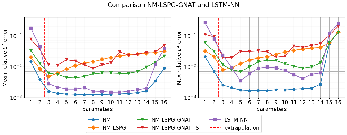
Figure 9: Comparison of the accuracies beetween all the ROMs presented on the test set of $N^{\mu}_{\text{test}}=16$ parameters, each associated to a time series of $N^{t}_{\text{test}}=101$ intermediate solutions. The number of magic points employed for NM-LSPG-GNAT and NM-LSPG-GNAT-TS is $150$. The mean and maximum relative $L^{2}$-errors are taken with respect to the time scale.

4.2 Shallow Water Equations (SWE)

The second test case we present is a 2d non-linear, time-dependent, parametric model based on the shallow water equations (SWE). Also in this case, the non-temporal parameter affects the initial conditions, $\mu\in[0.1,0.3]$:

$$\begin{cases}\partial_{t}(h\mathbf{u})+\nabla\cdot(h\mathbf{u}\otimes\mathbf{u})+\frac{1}{2}|\mathbf{g}|h\nabla h=0&(\mathbf{x},t)\in[0,1]^{2}\times[0,0.2],\\ \partial_{t}h+\nabla\cdot(\mathbf{u}h)=0&(\mathbf{x},t)\in[0,1]^{2}\times[0,0.2],\\ \mathbf{u}(\mathbf{x},0)=0&\mathbf{x}\in[0,1]^{2},\\ h(\mathbf{x},0)=\mu\left(\frac{1}{e^{1}}\cdot e^{-\frac{1}{0.04-\lVert\mathbf{x}-\mathcal{O}\rVert_{2}^{2}}}\chi_{\lVert\mathbf{x}\rVert_{2}^{2}<0.2}+\chi_{\lVert\mathbf{x}\rVert_{2}^{2}\geq 0.2}\right)&\mathbf{x}\in[0,1]^{2},\\ \mathbf{u}(\mathbf{x},t)\cdot\mathbf{n}=0&(\mathbf{x},t)\in\partial[0,1]^{2}\times[0,0.2],\\ \nabla h(\mathbf{x},t)\cdot\mathbf{n}=0&(\mathbf{x},t)\in\partial[0,1]^{2}\times[0,0.2],\end{cases}$$ (37)

where $h$ is the water depth, $\mathbf{u}$ is the velocity vector, $\mathbf{g}$ is the gravitational acceleration, and $\mathcal{O}$ is the point $(0.5,0.5)\in\Omega$. We consider a constant batimetry $h_{0}=0$, so that the free surface height $h_{\text{total}}=h+h_{0}$ is equal to the water depth $h$.

The time step that will be employed for the evolution of the dynamics of the FOM is $1\mathrm{e}-4$ seconds. The training and test snapshots are sampled every $4$ time steps. The training non-temporal parameters are $N^{\mu}_{\text{train}}=10$ in number and they are sampled equispacedly in the training interval $\mu\in[0.1,0.3]$, for a total of $N_{\text{train}}=N^{\mu}_{\text{train}}\cdot N^{t}_{\text{train}}=10\cdot 501=5010$ training snapshots.

Due to an inaccurate reconstruction erorr of the CAE for the first time instants, the predictions of the dynamics of the reduced model are evaluated from the time instant $t_{0}=0.01$ seconds. The test non-temporal parameters are $N^{\mu}_{\text{test}}=8$ in number and sampled equispacedly in the test interval $\mu\in[0.05,0.35]$, for a total of $N_{\text{test}}=N^{\mu}_{\text{test}}\cdot N^{t}_{\text{test}}=8\cdot 475=3800$ test snapshots, since the first $26$ are cut from the time series, $N^{t}_{\text{train}}=501$ snapshots long. Again the first $2$ and the last $2$ parameters correspond to the extrapolation regime. The initial latent variables are obtained projecting with the encoder into the latent space the test snapshots corresponding to the time instants $t_{0}=0.01$ instead of $t=0$. The training and test time series are labelled from $1$ to $10$ and from $1$ to $8$ with an increasing order.

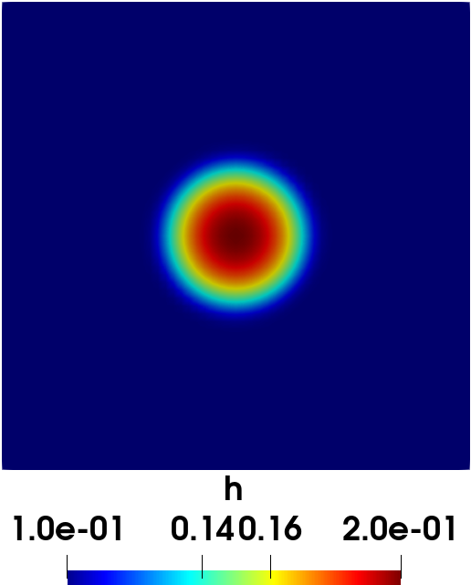
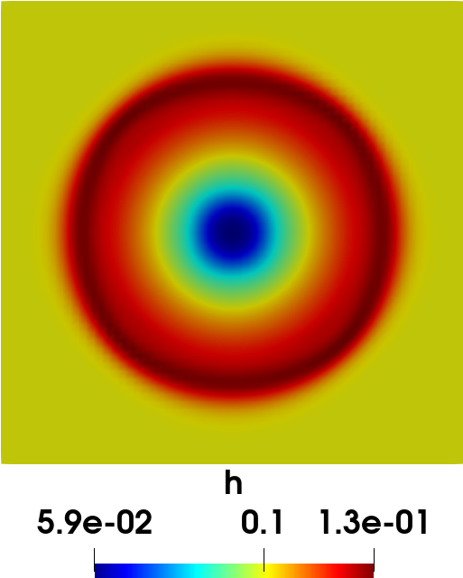
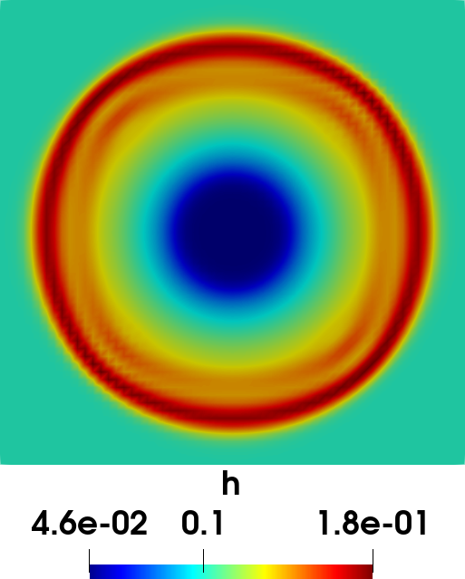
Figure 10: From left to right: FOM solution of equation 35 at $(t,\mu)\in\{(0.01,0.1),(0.2,0.1),(0.01,0.3),(0.2,0.3)\}$.

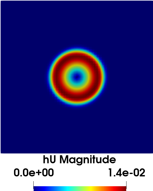
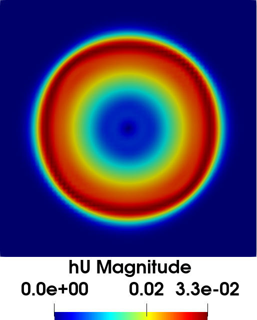
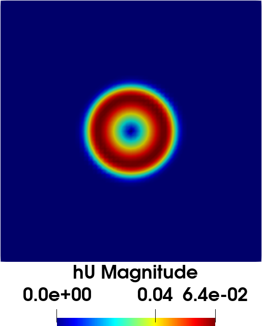
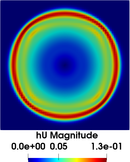
Figure 11: From left to right: FOM solution of equation 35 at $(t,\mu)\in\{(.010,0.1),(0.2,0.1),(0.01,0.3),(0.2,0.3)\}$.

In this test case the ROC hyper-reduction is more accurate with respect to the GNAT one, so the results are reported w.r.t. this hyper-reduction method.

4.2.1 Full-order model

One detail that we didn’t stress in the previous test case is that the FOM and the NM-LSPG ROM can discretize the residuals of the SWE differently: only the consistency of the discretization is required, characterizing the NM-LPSG family as equations-based rather than fully intrusive.

The FOM solutions are computed with the OpenFoam solver shallowWaterFoam [1], while the ROMs discretize the residual with a much simpler numerical scheme.

The FOM numerical scheme is the PIMPLE algorithm, a combination of PISO [45] (Pressure Implicit with Splitting of Operator) and SIMPLE [32] (Semi-Implicit Method for Pressure-Linked Equations). For the shallow water equations the free surface height $h$ plays the role of the pressure in the Navier-Stokes equations, regarding the PIMPLE algorithm implementation. The number of outer PISO corrections is $3$.

The time discretization is performed with the semi-implicit Euler method. The non-linear advection terms are discretized with the Linear-Upwind Stabilised Transport (LUST) scheme that requires a stencil with $2$ layers of adjacent cells for the hyper-reduction. The gradients are linearly interpolated through Gauss formula. The solutions for $hU$ are obtained with Gauss-Seidel iterative method, and for $h$ with the conjugate gradient method preconditioned by the Diagonal-based Incomplete Cholesky (DIC) preconditioner. For both of them the absolute tolerance on the residual is $1\mathrm{e}-6$ and the relative tolerance of the residual w.r.t. the initial condition is $0.1$.

The residual of ROMs is instead discretized as follows. If we represent with $M_{hU},\ M_{h}$ the mass matrices, with $G(h)$ the discrete gradient vector of $h$, and with $C_{hU}((hU)^{t-1}),\ C_{h}(U^{t-1})$ the advection matrices, then, at every time instant $t$, the discrete equations

$$\frac{M_{hU}}{\Delta t}(hU)^{t}+C_{hU}((hU)^{t-1})U^{t}+ghG(h)=\frac{M_{hU}}{\Delta t}(hU)^{t-1},$$ (38)

$$\frac{M_{h}}{\Delta t}h^{t}+C_{h}(U^{t-1})h^{t}=\frac{M_{h}}{\Delta t}h^{t-1},$$ (39)

are solved for the state $((hU)^{t},h^{t})$ with a semi-implicit Euler method. The same numerical schemes and linear systems iterative solvers of the FOM are employed. In principle, they could be changed.

Since now the stencil of a single cell needs two layers of adjacent cells for the discretizations, for each internal magic point, $12$ additional cells need to be considered for the hyper-reduction.

4.2.2 Manifold Learning

The CAE architecure for the SWE model is reported in Table 6. This time one encoder and two decoders, one for the velocity $U$ and one for the height $h$ are trained. Moreover, to increase the generalization capabilities we converted $2$ layers of the decoder for $U$ in recurrent convolutional layers as shown in the Appendix. Even with this modification the initial time steps, from $0$ to $0.01$ are associated to a high reconstruction error: the relative $L^{2}$-error is around $0.1$ for every test parameter at the initial time instants, slowly decreasing towards the accuracy shown in Figure 12 after $t=0.01$, chosen as initial instant from here onward.

The CAE is trained for $500$ epochs with a batch size of $20$ and an initial learning rate of $1\mathrm{e}-4$, that halves if the loss from Equation 12 does not decrease after $50$ epochs. In this case the state is $(U,h)$ so the encoder has three channels, two for the velocity components, $U_{1}$, $U_{2}$, and one for the height, $h$. The high computational cost is shown in Table 4. We have to observe that nor the architecture is parsimonious for a good approximation of the discrete solution manifold in the time interval $[0.01,0.2]$, neither the number of training snapshots $5010$ is optimized to reach the highest efficiency with the lowest computational cost. Our focus is obtaining a satisfactory reconstruction error in order to build up our ROMs.

The solution manifold parametrized by the decoder achieves the reconstruction error of a linear manifold spanned by around $20$ POD modes. In fact, the decay of the reconstruction error associated to the POD approximations is faster than the previous test case in the time interval $[0.01,0.2]$.

It can be seen from the representation of the latent dynamics associated to the train parameters in Figure 13, that the initial solutions overlap. This and the low accuracy could be explained by the fact that the FOM dynamics has different scales, especially for the velocity $U$ that from the initial constant zero solution reaches a magnitude of $10^{-1}$ meter per seconds. Further observations and possible solutions are presented in the Discussion section 5.

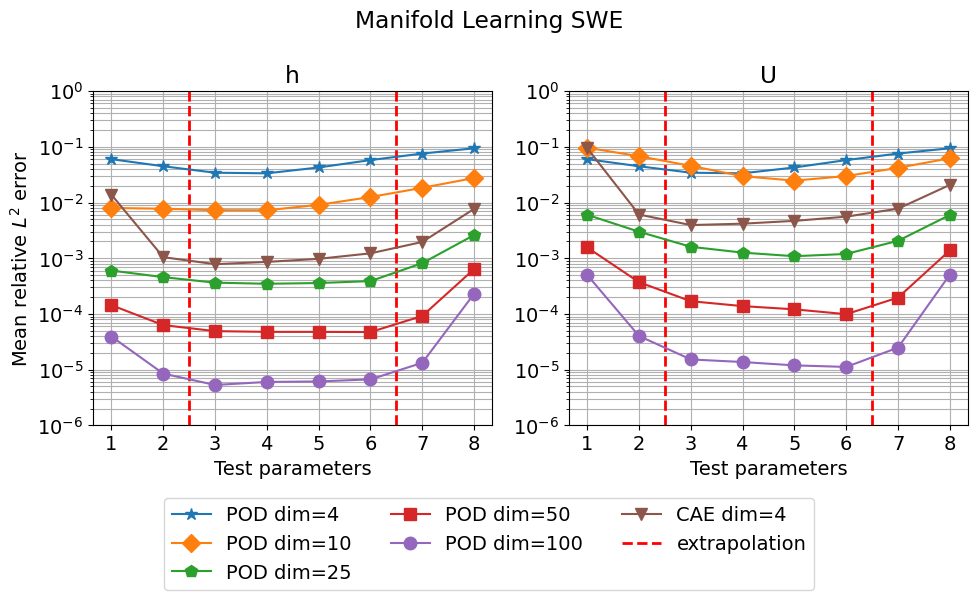
Figure 12: Comparison between the CAE’s and POD’s projection errors of the discrete solution manifold represented by the $N^{\text{train}}=N^{\mu}_{\text{train}}\cdot N^{t}_{\text{train}}=10\cdot 501=5010$ training snapshots. The error is evaluated on the $8$ test parameters, each associated with a time series of $N^{t}_{\text{test}}=475$, for a total of $N_{\text{test}}=3800$ test snapshots. The mean is performed over the time scale.

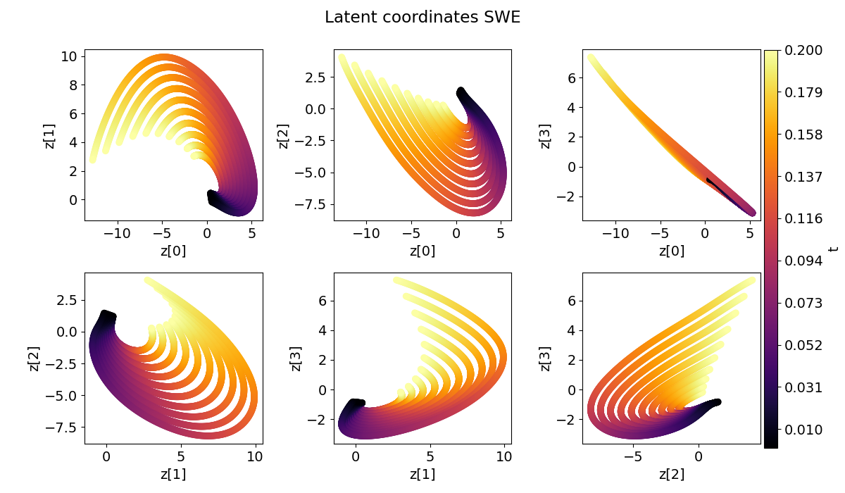
Figure 13: Correlations among the $4$ latent coordinates of the train set, $10$ in total. They are obtained projecting the train snapshots into the latent space of the CAE with the encoder. The coloring corresponds to the time instants from $0.$ to $0.2$, with a time step of $4\mathrm{e}-4$ seconds. The initial time steps employed in the ROMs is $0.01$ seconds.

4.2.3 Hyper-reduction and teacher-student training

Mimicking the structure of the CAE, the compressed decoder is split in two, one for the velocity $U$ and one for the free surface height $h$. The architecture for both the decoders is a feed-forward NN with a single hidden layer; they are reported in the Table 8. The compressed decoders are trained for $1500$ epochs, with a batchsize of $20$, and an initial learning rate of $1\mathrm{e}-4$ that halves after $100$ epochs if the loss does not decreases, with a minimum value of $1\mathrm{e}-6$. As for the previous test case, the number of magic points, hidden layer sizes, training times, average training epoch computational cost are reported in Table 3. This time for each magic point correspond $3$ degrees of freedom, so the actual output dimension of the compressed decoders is three times the submesh sizes.

The relative $L^{\infty}$-error of the compressed decoder is shown in Figure 14. This time the extrapolation error is sensibly higher as already seen in the reconstruction error of the CAE.

Table 3: In this table are reported for the SWE test case: the submesh size and the hidden layer (HL) number of nodes of the compressed decoder; the Teacher-Student training (TS) duration in secods, the Teacher-Student training average epoch duration in seconds; the average time step for NM-LSPG-GNAT with compressed decoder (GNAT-TS) in milliseconds, and the average time step for NM-LSPG-GNAT with the hyper-reduced residuals but full CAE decoder (GNAT-no-TS) in milliseconds. In red the average computational cost with $13$ maximum residual evaluations due to the instability in the evolution of the dynamics of the test parameter $4$.

MP	Submesh size	HL size	TS total epochs	TS avg epoch	avg GNAT-TS	avg GNAT-no-TS
25	238	600	582 [s]	0.388432 [s]	3.227 [ms]	14.782 [ms]
50	345	600	1234 [s]	0.823084 [s]	4.062 [ms]	13.742 [ms]
100	590	900	6428 [s]	4.285968 [s]	4.387 [ms]	15.238/22.688 [ms]
150	654	900	6746 [s]	4.497579 [s]	4.307 [ms]	14.307 [ms]

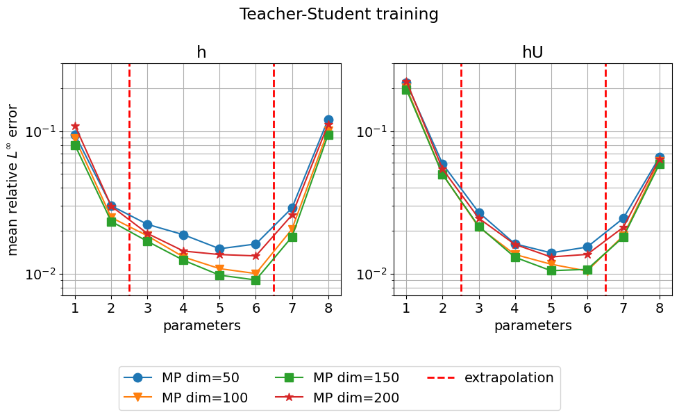
Figure 14: Prediction accuracy on the test snapshots restricted to the magic points. The accuracy is measured with the relative $L^{\infty}$-error averaged over the time trajectories associated to each one of the $N^{\mu}_{\text{test}}=8$ test samples.

As in the previous case, both the NM-LSPG-ROC and NM-LSPG-ROC-TS ROMs are considered. This time it’s the NM-LSPG-ROC’s dynamics to be less stable with $7$ maximum residual evaluations of the LM algorithm. In this respect, for parameter test $4$ and $\text{mp}=100$ the maximum number of residual evaluations is increased to $13$; in the error plots in Figures 15 and 16, only the value for parameter $4$, $\text{mp}=100$ is substituted. It is relevant to notice that the extrapolation error is lower for higher numbers of magic points and for the NM-LSPG-ROC method.

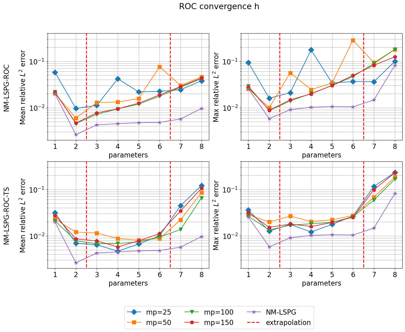
Figure 15: First row: NM-LSPG-ROC mean and max relative $L^{2}$-error. Second row: NM-LSPG-ROC-TS mean and max relative $L^{2}$-error. In violet also the NM-LSPG accuracy is reported. The mean and max values are evaluated with respect to the time series of intermediate solutions associated to each one of the $8$ test parameters.

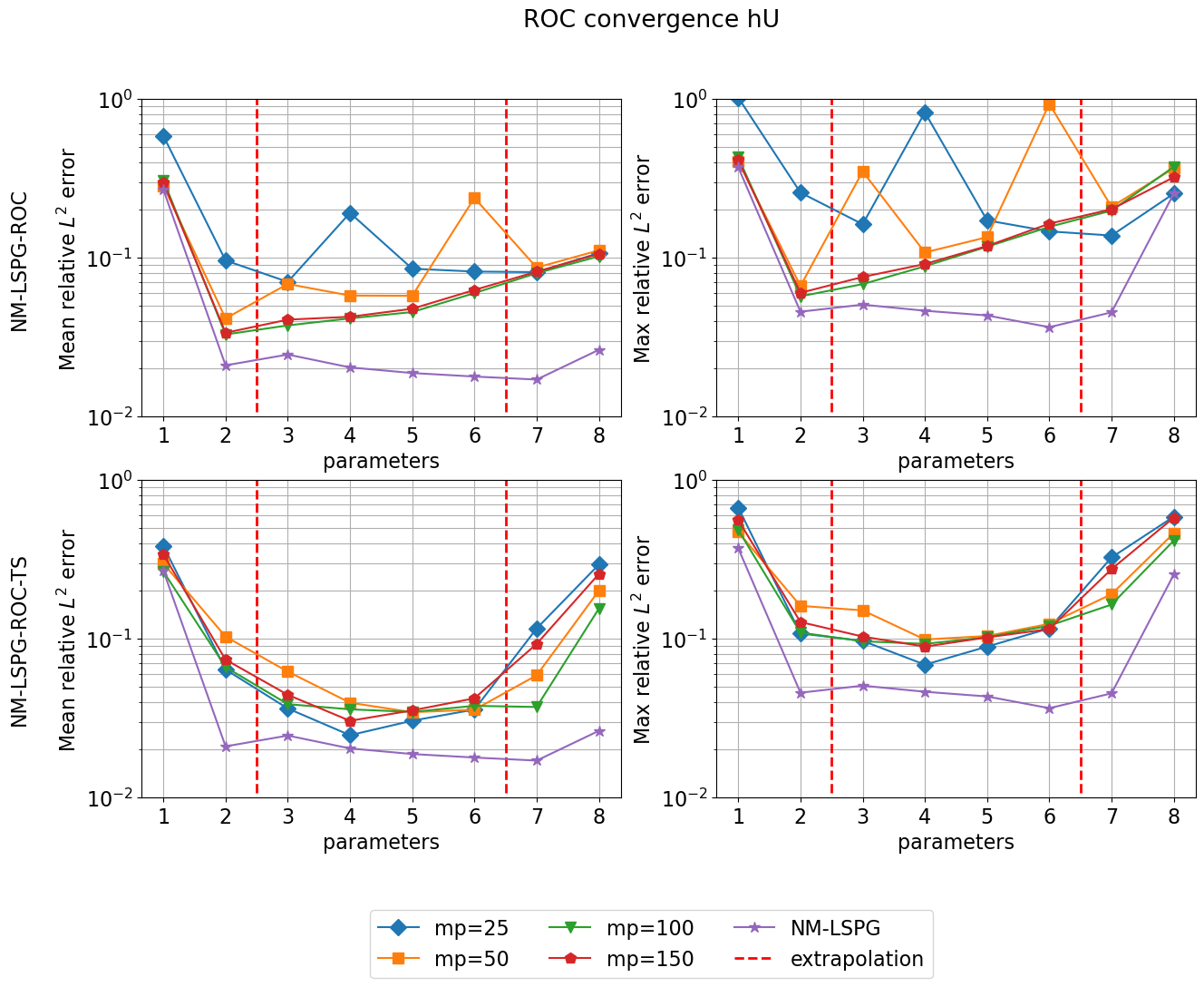
Figure 16: First row: NM-LSPG-ROC mean and max relative $L^{2}$-error. Second row: NM-LSPG-ROC-TS mean and max relative $L^{2}$-error. In violet also the NM-LSPG accuracy is reported. The mean and max values are evaluated with respect to the time series of intermediate solutions associated to each one of the $8$ test parameters.

4.2.4 Comparison with data-driven predictions based on LSTM

The same LSTM architecture of the NCL test case is trained with the same training procedure, only that now there are $5010$ training parameters-latent coordinates pairs. For the architecture’s specifics see Table 9. The computational costs introduced in the previous test case are reported also for the SWE model in Table 4.

With the architecture and training procedure employed, the LSTM could not achieve a good accuracy at the initial time instants after $t_{0}=0.01$ seconds: for this reason in the plot of the errorsini Figure 17 is reported both the mean over the whole test time series of $475$ elements and over the time series after the $40$-th element of the $475$, that corresponds to the the time instant $0.017$ seconds. This issue should be ascribed at what we discussed about in subsection 4.2.2, about the latent dynamics overlappings. Further remarks are provided in the Discussion section 5.

A part from this, the LSTM predictions are for almost every test parameter above only the NM-LSPG and CAE’s reconstruction errors. Even in the extrapolation regimes, the predictions are more accurate than the NM-LSPG-ROC and NM-LSPG-ROC-TS reduced-order models. Regarding the computational costs, this time not only the LSTM model but also the NM-LSPG-ROC-TS ROMs achieve a little speed-up w.r.t. the FOM. The choice of doubling the decoders has repercussions in the online costs, but it was made only in an effort to reach a good reconstruction error of the CAE; maybe more light architectures could be employed for the restricted time interval $[0.01,0.2]$.

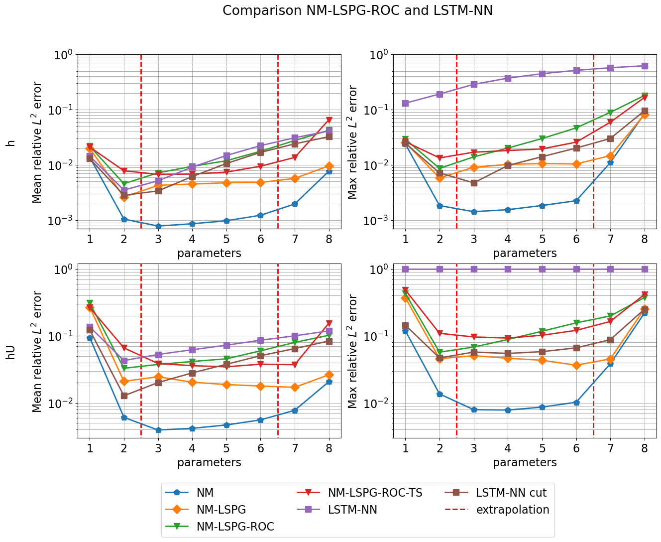
Figure 17: Comparison of the accuracies between all the ROMs presented on the test set of $8$ parameters, each associated to a time series of $475$ intermediate solutions. The number of magic points employed for NM-LSPG-ROC and NM-LSPG-ROC-TS is $100$. The mean and maximum relative $L^{2}$-errors are taken with respect to the time scale. Since the LSTM is inaccurate between the time instants $0.01$ and $0.017$ seconds we report also the mean over the time interval $[0.017,\ 0.2]$ witch label ’LSTM-NN cut’, to establish a fair comparison.

Table 4: Offline stage: full-order model (FOM) computation of the $5010$ snapshots, average cost of a single epoch for the training of the CAE with a batch size of $20$, and total cost for $500$ epochs; average epoch’s cost for the LSTM training with a batch size of $100$, and total cost for $10000$ epochs. Online stage: for the FOM, NM-LSPG and LSTM-NN models it is reported the average of a single time step cost over all the $8$ test parameters and time series, and the average cost of the full dynamics over the $8$ test parameters. The LSTM-NN full-dynamics is evaluated with a single forward.

Offline stage	Time
FOM snapshots evaluation	137.079881 [s]
CAE training single epoch avg	94.700484 [s]
CAE training	51431 [s]
LSTM-NN training single epoch avg	0.107722 [s]
LSTM-NN training	1076.150 [s]

Online stage	Time
avg FOM time step	7.251 [ms]
avg FOM full dynamics	116.024578 [s]
avg NM-LSPG time step	22.126 [ms]
avg NM-LSPG full-dynamics	336.171916 [s]
avg LSTM-NN time step	1.802 [ms]
avg LSTM-NN full-dynamics	6.834247 [s]

5 Discussion

We comment the numerical results obtained:

• Computational cost of the CAEs training. It is evident from Tables 2 and 7 that the offline stage’s computational cost is dominated by the CAEs trainings. We have to remark that the architectures were not optimized to be the most persimonious ones in order to achieve the desired reconstruction error. Moreover, libtorch training took almost twice more time than the same architecture’s training in PyTorch, due to implementation inconsistencies. The cost of the forward evaluations of the decoder are comparable instead, not changing much the online costs. The training of the CAEs could be furtherly reduced with transfer learning [26] or preprocessing steps that enlight some features of the dynamics that are more easily learnable, as was done in [24]. Also the number of training snapshots could be optimized furtherly for the test cases presented. The same observations apply also for the compressed decoders. Moreover, a parallel implementation of the training procedures on more than one GPU is mandatory to achieve competitive computational costs.

• Simultaneous CAE and compressed decoder/LSTM training. The additional costs of the LSTM and compressed decoder training could be cut with a unified training of the CAE and compressed decoder: after some epochs, the training of the LSTM or compressed decoder could be switched on and performed at the same time of the CAE’s since the only additional information, a part from the restriction of the snapshots into the magic points, is the latent dynamics coordinates learned anyway during the CAE’s optimization.

• Increasing the speed-up of the non-linear manifold ROMs. The bottleneck for the efficiency of the NM-LSPG-ROC-TS and NM-LSPG-ROC ROMs in the online stage is the cost of the compressed decoder or CAE’s decoder forward. Regarding the NLC model, our results for the average time step of the NM-LPSG-GNAT-TS and NM-LSPG-GNAT ROMs from Table 1 are comparable if not lower than the approximate time step of $7-8$ milliseconds for the NM-LSPG-GNAT with shallow autoencoders ROM presented in [33]. The difference is that now the FOM implemented with the FVM in OpenFoam [1] takes $2.42$ seconds for $2000$ time steps instead of $140.67$ seconds for $1500$ time steps in [33] with finite differences for a smilar test case, i.e. 2d burgers equation instead of our non-linear conservation law. To show a more consistent speed-up w.r.t. the FOM, as for the SWE test case, the number of degrees of freedom could be increased without influencing the NM-LSPG-ROC-TS ROM since it is not dependent on the FOM’s dimension. In a weaker sense also the NM-LSPG-ROC ROM is also independent on the number of degrees of freedom of the FOM, a part from the weights of the CAE’s decoder that concur in increasing the cost of a single forward in the online stage.

• Generalization error of LSTM and CAE and additional inductive biases. The generalization error of the NN employed depends on a lot of factors, from the number of training samples to the regularization term in the loss, the architectures, etc. It is thus difficult to predict how much the accuracy of the predictions will decay outside the training range. Adding a physics-informed term in the loss of the CAE does not provide an improvement of the reconstruction error if enough training data are employed as in our test cases. Some regularization properties could be imposed in the latent dynamics to facilitate the evolution of the NM-LPSG-ROC ROMs, for example imposing a linear latent dynamics could be beneficial

• Purely data-driven LSTM ROM vs NM-LSPG-ROC and NM-LSPG-ROC-TS ROMs. One crucial difference is interpretability: in the first case, the latent dynamics is obtained training the LSTM to approximate the latent coordinates, in the second case, the latent dynamics is evolved in time minimizing the hyper-reduced residual based on the physical model’s equations. Regarding the LSTM predictions, we have seen in the test cases that despite the higher accuracy in the training range and the low computational online cost, there might be other issues in the extrapolation regime: in the NLC test case, the accuracy was sensitively lower in the extrapolation regime, even if it could be improved in theory increasing the layers and nodes of the LSTM in exchange for a higher training cost; in the SWE test case the initial time step from $0.01$ to $0.017$ seconds could not be well-approximated due to different scales and overlappings in the latent dynamics. The NM-LSPG-ROC and NM-LSPG-ROC-TS mitigated in some sense these issues, delegating less effort in the tuning of the hyper-parameters of the LSTM and increasing the interpretability of the results. Moreover the LSTM NN, approximate the dynamics only every time step imposed by the training input-output pairs, while the non-linear manifold ROMS, can in principle approximate the latent dynamics with an arbitrarly small time step, since the decoder provides a continuous approximation of the solution manifold and the dynamics is evolved based on a numerical scheme with changable time step. With respect to purely data-driven methods though, non-linear manifold methods require a lower reconstruction error of the CAE since every successive ROMs’ dynamics evolution depends on how well the intermediate solutions are reconstructed through the decoder.

• Learn the solution manifolds with autoencoders in unstructured meshes. The natural question of how to extend the CAE architecture to 3D or unstructured meshes, is being currently studied. In the literature there are already interesting results that employ graph neural networks and their variants to find latent representations of 3d simulations [46].

6 Conclusions and perspectives

We have developed two new hyper-reduced non-linear manifold ROMs: NM-LSPG-ROC and NM-LSPG-ROC-TS, that can be converted in NM-LSPG-GNAT and NM-LSPG-GNAT-TS. In NM-LPSG-ROC-TS the residuals of the NM-LSPG ROM are hyper-reduced with over-collocation, while the decoder of the CAE is approximated with teacher-student training into a compressed decoder. In NM-LSPG-ROC only the residuals’ hyper-reduction is carried out. The methods perform similarly in accuracy and computational cost w.r.t. the NM-LSPG-GNAT with shallow autoencoders ROM introduced in [33], for a similar test case. The flexibility of our method permits to change the CAE architecture depending on the problem at hand, without imposing too many constraints on its structure, in order to reach the convergence faster and achieve a lower reconstruction error.

With respect to purely data-driven ROMs built on the CAE’s solution manifold, NM-LSPG-ROC and NM-LSPG-ROC-TS provide more interpretable and, in the extrapolation regimes, sometimes more accurate predictions, and they need less hyper-parameters tuning, once the CAE is trained. Moreover, the methods devolped are equations-based rather than fully-intrusive, and exploit the physics of the model to evolve the latent dynamics. It is crucial, though, that the CAE’s reconstruction error is sufficiently low, since the latent dynamics needs to be computed with numerical schemes that rely on the accuracy of the reconstructed solutions through the decoder of the CAE or the compressed decoder. We base this observations on the results obtained for two parametric non-linear time-dependent benchmarks presented in the numerical results section 4, that is a 2d non-linear conservation law model (NLC) and a 2d shallow water equations model. Despite the speed-up is not achieved or not significant with respect to the FOMs, we reached satisfactory results in terms of the accuracy and the latent or reduced dimension of the ROMs.

Future directions involve the implementation of the developed ROMs in real applications with higher computational costs and degrees of freedom, such that a more evident speed-up is reached. This may involve the developement of autoencoders for more general mesh-based simulations, rather than orthogonal grids.

Appendix A Neural networks’ architectures

The architectures of the CAEs are shown in Tables 5, 6, of the compressed decoders in Tables 7 and 8, and of the LSTMs in Table 9. We mainly employ the Exponential Linear Unit (ELU) and Rectified Linear Unit (ReLU) activation functions. The padding is symmetric. The labels Conv2d, ConvTr2d and ConvTr2dRec, stand for 2d convolutions, transposed 2d convolutions [44], and 2d transposed convolution associated to a recurrent layer, i.e. they are summed to the previous layer and then passed to an ELU activation function.

Table 5: Nonlinear Conservation Law model’s Convolutional Autoencoder.

Encoder	Activation	Weights	Padding
Conv2d	ELU	[2, 8, 5, 5]	0
Conv2d	ELU	[8, 16, 3, 3]	1
Conv2d	ELU	[16, 32, 3, 3]	1
Conv2d	ELU	[32, 64, 3, 3]	1
Conv2d	ELU	[64, 128, 2, 2]	1
Linear	ELU	[1152, 4]	-

Decoder	Activation	Weights	Padding
Linear	ELU	[4, 1152]	-
ConvTr2d	ELU	[128, 64, 2, 2]	1
ConvTr2d	ELU	[64, 32, 3, 3]	1
ConvTr2d	ELU	[32, 16, 4, 4]	1
ConvTr2d	ELU	[16, 8, 4, 4]	0
ConvTr2d	ReLU	[8, 2, 4, 4]	1

Table 6: Shallow Water Equations model’s Convolutional Autoencoder. The decoder for $U$ has two recurrent layers.

Encoder	Activation	Weights	Padding
Conv2d	ELU	[2, 8, 5, 5]	0
Conv2d	ELU	[8, 16, 3, 3]	1
Conv2d	ELU	[16, 32, 3, 3]	1
Conv2d	ELU	[32, 64, 3, 3]	1
Conv2d	ELU	[64, 128, 2, 2]	1
Linear	ELU	[1152, 4]	-

Decoder h	Activation	Weights	Padding
Linear	ELU	[4, 1152]	-
ConvTr2d	ELU	[240, 120, 2, 2]	1
ConvTr2d	ELU	[120, 60, 3, 3]	1
ConvTr2d	ELU	[60, 30, 4, 4]	1
ConvTr2d	ELU	[30, 15, 4, 4]	0
ConvTr2d	ReLU	[15, 1, 4, 4]	1

Decoder U	Activation	Weights	Padding
Linear	ELU	[4, 2700]	-
ConvTr2d	ELU	[300, 75, 2, 2]	1
ConvTr2d	ELU	[150, 75, 3, 3]	1
ConvTr2dRec	-	[150, 75, 3, 3]	1
ConvTr2d	ELU	[75, 35, 4, 4]	1
ConvTr2d	ELU	[35, 20, 4, 4]	0
ConvTr2dRec	-	[35, 20, 4, 4]	0
ConvTr2d	-	[20, 2, 4, 4]	1

Table 7: Nonlinear Conservation Law model’s Compressed Decoders.

Magic Points	$1^{st}$ layer weight	$1^{st}$ layer activation	$2^{nd}$ layer weight	$2^{nd}$ layer activation
50	[4, 300]	ELU	[300, 278]	ReLU
100	[4, 350]	ELU	[350, 492]	ReLU
150	[4, 400]	ELU	[400, 670]	ReLU

Table 8: Shallow Water Equations model’s Compressed Decoders: height $h$ and velocity $U$ in order.

Magic Points	$1^{st}$ layer weight	$1^{st}$ layer activation	$2^{nd}$ layer weight	$2^{nd}$ layer activation
25	[4, 200]	ELU	[200, 238]	ReLU
50	[4, 200]	ELU	[200, 345]	ReLU
100	[4, 300]	ELU	[300, 590]	ReLU
150	[4, 300]	ELU	[300, 654]	ReLU

Magic Points	$1^{st}$ layer weight	$1^{st}$ layer activation	$2^{nd}$ layer weight	$2^{nd}$ layer activation
25	[4, 400]	ELU	[400, 478]	-
50	[4, 400]	ELU	[400, 960]	-
100	[4, 600]	ELU	[600, 1180]	-
150	[4, 600]	ELU	[600, 1308]	-

Table 9: Nonlinear Conservation Law model’s and Shallow Water Equations model’s Long-Shot Term Memory Neural Network.

	input dim	output dim	number of LSTM layers
LSTM layer	2	100	2

	$1^{st}$ layer weight	$1^{st}$ layer activation	$2^{nd}$ layer weight	$2^{nd}$ layer activation
Linear encoding layer	[100, 50]	ELU	[50, 4]	-

References

- [1] OpenFOAM Documentation Website. https://www.openfoam.com.
- [2] D. Amsallem and C. Farhat. Interpolation method for adapting reduced-order models and application to aeroelasticity. AIAA journal, 46(7):1803–1813, 2008.
- [3] I. Babuška, F. Nobile, and R. Tempone. A stochastic collocation method for elliptic partial differential equations with random input data. SIAM Journal on Numerical Analysis, 45(3):1005–1034, 2007.
- [4] N. Baker, F. Alexander, T. Bremer, A. Hagberg, Y. Kevrekidis, H. Najm, M. Parashar, A. Patra, J. Sethian, S. Wild, et al. Workshop report on basic research needs for scientific machine learning: Core technologies for artificial intelligence. Technical report, USDOE Office of Science (SC), Washington, DC (United States), 2019.
- [5] M. Barrault, Y. Maday, N. C. Nguyen, and A. T. Patera. An ‘empirical interpolation’method: application to efficient reduced-basis discretization of partial differential equations. Comptes Rendus Mathematique, 339(9):667–672, 2004.
- [6] P. Benner, M. Ohlberger, A. Cohen, and K. Willcox. Model reduction and approximation: theory and algorithms. SIAM, 2017.
- [7] F. Bernard, A. Iollo, and S. Riffaud. Reduced-order model for the BGK equation based on POD and optimal transport. Journal of Computational Physics, 373:545–570, 2018.
- [8] S. Bhattacharjee and K. Matouš. A nonlinear manifold-based reduced order model for multiscale analysis of heterogeneous hyperelastic materials. Journal of Computational Physics, 313:635–653, 2016.
- [9] M. M. Bronstein, J. Bruna, Y. LeCun, A. Szlam, and P. Vandergheynst. Geometric deep learning: going beyond euclidean data. IEEE Signal Processing Magazine, 34(4):18–42, 2017.
- [10] M. Buffoni, H. Telib, and A. Iollo. Iterative methods for model reduction by domain decomposition. Computers & Fluids, 38(6):1160–1167, 2009.
- [11] K. Carlberg, C. Bou-Mosleh, and C. Farhat. Efficient non-linear model reduction via a least-squares Petrov–Galerkin projection and compressive tensor approximations. International Journal for numerical methods in engineering, 86(2):155–181, 2011.
- [12] K. Carlberg, C. Farhat, J. Cortial, and D. Amsallem. The GNAT method for nonlinear model reduction: Effective implementation and application to computational fluid dynamics and turbulent flows. Journal of Computational Physics, 242:623–647, Jun 2013.
- [13] K. Carlberg, C. Farhat, J. Cortial, and D. Amsallem. The GNAT method for nonlinear model reduction: effective implementation and application to computational fluid dynamics and turbulent flows. Journal of Computational Physics, 242:623–647, 2013.
- [14] S. Chaturantabut and D. C. Sorensen. Nonlinear model reduction via discrete empirical interpolation. SIAM Journal on Scientific Computing, 32(5):2737–2764, 2010.
- [15] Y. Chen, S. Gottlieb, L. Ji, and Y. Maday. An EIM-degradation free reduced basis method via over collocation and residual hyper reduction-based error estimation. arXiv preprint arXiv:2101.05902, 2021.
- [16] Y. Choi and K. Carlberg. Space–time least-squares Petrov–Galerkin projection for nonlinear model reduction. SIAM Journal on Scientific Computing, 41(1):A26–A58, 2019.
- [17] Y. Choi, D. Coombs, and R. Anderson. SNS: a solution-based nonlinear subspace method for time-dependent model order reduction. SIAM Journal on Scientific Computing, 42(2):A1116–A1146, 2020.
- [18] A. Cohen and R. DeVore. Kolmogorov widths under holomorphic mappings. IMA Journal of Numerical Analysis, 36(1):1–12, 2016.
- [19] R. A. DeVore, R. Howard, and C. Micchelli. Optimal nonlinear approximation. Manuscripta mathematica, 63(4):469–478, 1989.
- [20] P. Díez, A. Muixí, S. Zlotnik, and A. García-González. Nonlinear dimensionality reduction for parametric problems: a kernel Proper Orthogonal Decomposition (kPOD). arXiv preprint arXiv:2104.13765, 2021.
- [21] M. Finzi, S. Stanton, P. Izmailov, and A. G. Wilson. Generalizing convolutional neural networks for equivariance to lie groups on arbitrary continuous data. In International Conference on Machine Learning, pages 3165–3176. PMLR, 2020.
- [22] N. R. Franco, A. Manzoni, and P. Zunino. A Deep Learning approach to Reduced Order Modelling of Parameter Dependent Partial Differential Equations. arXiv preprint arXiv:2103.06183, 2021.
- [23] T. Franz, R. Zimmermann, S. Görtz, and N. Karcher. Interpolation-based reduced-order modelling for steady transonic flows via manifold learning. International Journal of Computational Fluid Dynamics, 28(3-4):106–121, 2014.
- [24] S. Fresca and A. Manzoni. POD-DL-ROM: enhancing deep learning-based reduced order models for nonlinear parametrized PDEs by proper orthogonal decomposition. Computer Methods in Applied Mechanics and Engineering, 388:114181, 2022.
- [25] D. Geller and I. Z. Pesenson. Kolmogorov and linear widths of balls in Sobolev spaces on compact manifolds. Mathematica Scandinavica, pages 96–122, 2014.
- [26] I. Goodfellow, Y. Bengio, and A. Courville. Deep learning. MIT press, 2016.
- [27] J. Gou, B. Yu, S. J. Maybank, and D. Tao. Knowledge distillation: A survey. International Journal of Computer Vision, 129(6):1789–1819, 2021.
- [28] P. Goyal and P. Benner. LQResNet: A Deep Neural Network Architecture for Learning Dynamic Processes. arXiv preprint arXiv:2103.02249, 2021.
- [29] C. Greif and K. Urban. Decay of the Kolmogorov N-width for wave problems. Applied Mathematics Letters, 96:216–222, 2019.
- [30] G. Guennebaud, B. Jacob, et al. Eigen v3. http://eigen.tuxfamily.org, 2010.
- [31] J. S. Hesthaven, G. Rozza, B. Stamm, et al. Certified reduced basis methods for parametrized partial differential equations, volume 590. Springer, 2016.
- [32] R. Issa, B. Ahmadi-Befrui, K. Beshay, and A. Gosman. Solution of the implicitly discretised reacting flow equations by operator-splitting. Journal of computational physics, 93(2):388–410, 1991.
- [33] Y. Kim, Y. Choi, D. Widemann, and T. Zohdi. A fast and accurate physics-informed neural network reduced order model with shallow masked autoencoder. arXiv preprint arXiv:2009.11990, 2020.
- [34] D. P. Kingma and J. Ba. Adam: A method for stochastic optimization. arXiv preprint arXiv:1412.6980, 2014.
- [35] T. Lassila, A. Manzoni, A. Quarteroni, and G. Rozza. Generalized reduced basis methods and n-width estimates for the approximation of the solution manifold of parametric PDEs. In Analysis and numerics of partial differential equations, pages 307–329. Springer, 2013.
- [36] K. Lee and K. Carlberg. Deep Conservation: A latent dynamics model for exact satisfaction of physical conservation laws. arXiv preprint arXiv:1909.09754, 2019.
- [37] K. Lee and K. T. Carlberg. Model reduction of dynamical systems on nonlinear manifolds using deep convolutional autoencoders. Journal of Computational Physics, 404:108973, 2020.
- [38] W. Li, M. Zhen, and J. Yaolin. Model order reduction based on galerkin kpod for partial differential equations with variable coefficients. Journal on Numerica Methods and Computer Applications, 42(3):226, 2021.
- [39] D. J. Lucia, P. I. King, and P. S. Beran. Reduced order modeling of a two-dimensional flow with moving shocks. Computers & Fluids, 32(7):917–938, 2003.
- [40] N. T. Mücke, S. M. Bohté, and C. W. Oosterlee. Reduced Order Modeling for Parameterized Time-Dependent PDEs using Spatially and Memory Aware Deep Learning. Journal of Computational Science, page 101408, 2021.
- [41] K. P. Murphy. Machine learning: a probabilistic perspective. MIT press, 2012.
- [42] M. Ohlberger and S. Rave. Reduced basis methods: Success, limitations and future challenges. arXiv preprint arXiv:1511.02021, 2015.
- [43] D. Papapicco, N. Demo, M. Girfoglio, G. Stabile, and G. Rozza. The neural network shifted-proper orthogonal decomposition: A machine learning approach for non-linear reduction of hyperbolic equations, Mar. 2022.
- [44] A. Paszke, S. Gross, F. Massa, A. Lerer, J. Bradbury, G. Chanan, T. Killeen, Z. Lin, N. Gimelshein, L. Antiga, A. Desmaison, A. Kopf, E. Yang, Z. DeVito, M. Raison, A. Tejani, S. Chilamkurthy, B. Steiner, L. Fang, J. Bai, and S. Chintala. PyTorch: An Imperative Style, High-Performance Deep Learning Library. In H. Wallach, H. Larochelle, A. Beygelzimer, F. d'Alché-Buc, E. Fox, and R. Garnett, editors, Advances in Neural Information Processing Systems 32, pages 8024–8035. Curran Associates, Inc., 2019.
- [45] S. V. Patankar and D. B. Spalding. A calculation procedure for heat, mass and momentum transfer in three-dimensional parabolic flows. In Numerical prediction of flow, heat transfer, turbulence and combustion, pages 54–73. Elsevier, 1983.
- [46] T. Pfaff, M. Fortunato, A. Sanchez-Gonzalez, and P. W. Battaglia. Learning Mesh-Based Simulation with Graph Networks. arXiv preprint arXiv:2010.03409, 2020.
- [47] F. Pichi, F. Ballarin, G. Rozza, and J. S. Hesthaven. An artificial neural network approach to bifurcating phenomena in computational fluid dynamics, 2021.
- [48] A. Quarteroni, A. Manzoni, and F. Negri. Reduced basis methods for partial differential equations: an introduction, volume 92. Springer, 2015.
- [49] A. Quarteroni, R. Sacco, and F. Saleri. Matematica numerica. Springer Science & Business Media, 2010.
- [50] B. Smets, J. Portegies, E. Bekkers, and R. Duits. PDE-based group equivariant convolutional neural networks. arXiv preprint arXiv:2001.09046, 2020.
- [51] G. Stabile and R. Gianluigi. ITHACA-FV-in Real Time Highly Advanced Computational Applications for Finite Volumes.
- [52] G. Stabile, M. Zancanaro, and G. Rozza. Efficient geometrical parametrization for finite-volume-based reduced order methods. International Journal for Numerical Methods in Engineering, 121(12):2655–2682, 2020.
- [53] V. N. Temlyakov. Nonlinear Kolmogorov widths. Mathematical Notes, 63(6):785–795, 1998.
- [54] D. Torlo. Model reduction for advection dominated hyperbolic problems in an ALE framework: Offline and online phases. arXiv preprint arXiv:2003.13735, 2020.
- [55] J. Xu and K. Duraisamy. Multi-level convolutional autoencoder networks for parametric prediction of spatio-temporal dynamics. Computer Methods in Applied Mechanics and Engineering, 372:113379, 2020.