Minimax Risk in Estimating Kink Threshold and Testing Continuity

Abstract

We derive a risk lower bound in estimating the threshold parameter without knowing whether the threshold regression model is continuous or not. The bound goes to zero as the sample size $n$ grows only at the cube root rate. Motivated by this finding, we develop a continuity test for the threshold regression model and a bootstrap to compute its p-values. The validity of the bootstrap is established, and its finite sample property is explored through Monte Carlo simulations.

JEL Classification: C12, C13, C24.

Keywords: Continuity Test, Kink, Risk lower bound, Unknown Threshold.

1 INTRODUCTION

The threshold model has been widely used to model the nonlinearity of time series. For instance, threshold autoregressive (TAR) model is one of the earliest regime switching models. In its simplest form, it is assumed that there are two regimes. The regime is determined depending on the realization of the threshold variable and the threshold level. See Tong (1990) for a review. Hansen (2000) has extended it to the regression with more Economics application and Hansen and Seo (2002) and Seo (2006) to the threshold cointegration. Park and Shintani (2016) and Seo (2008) examined testing issues surrounding threshold effect and unit root. Chang et al. (2017) proposed an interesting generalization by introducing a latent factor threshold variable, while Lee et al. (2021) extended it further by estimating the factors from an external big data set.

Once one accepts the hypothesis of a threshold effect in the regression function via any of the available tests, see, e.g., Hansen (1996) and Lee et al. (2011) among others, one is then interested in deciding whether the “segmented” regression model is a model with a discontinuity (jump) or a model with a kink, since the so-called break/threshold tests are unable to discriminate between the two models. A powerful reason to test for a kink comes from the statistical inferential point of view. As we discuss in Section 2, the kink design can be represented by a set of restrictions on the parameter space of the threshold regression model. Thus, the parameters can be consistently estimated by the unrestricted least squares estimator. Unlike in the linear regression model, where one can make valid inferences based on the unconstrained estimation without knowing if the constraint holds, inferences in our context have very different statistical properties under the kink design when using the unrestricted estimation. More specifically, Hidalgo et al. (2019) shows that the rate of convergence of the estimate of the threshold point via unrestricted least squares method is $n^{1/3}$ if there is a kink, which is in contrast to $n^{1/2}$-rate when the (true) constraint of a kink is employed in its estimation (Feder, 1975; Chan and Tsay, 1998). If there is not a kink but a jump, then the unrestricted estimate converges in $n$-rate (Chan, 1993), which is also a $\ell_{1}$-minimax rate (Korostelev, 1987).

On the other hand, we may focus on the fact that the worst-case convergence rate of unrestricted estimate slows down to $n^{1/3}$ if the type of threshold is unknown compared with the situation in which the type of threshold is known so that it is used in the estimation. We show in Section 3 that the cube root convergence rate cannot be improved in terms of $\ell_{1}$-risk if the model does not specify the type of threshold. We extend these results to the diminishing threshold model, where the threshold degenerates in polynomial order. The diminishing threshold was introduced by Hansen (2000), and it can be understood as an asymptotic approximation of a small threshold. By allowing the diminishing threshold, we investigate how the size of the threshold affects the performance of estimators. Also, we develop a test valid under both fixed and diminishing threshold effect.

The main contribution of this paper is to develop a testing procedure to distinguish between jump and kink designs. Hansen (2017) considers inference under the kink design and mentioned “one could imagine testing the assumption of continuity within the threshold model class. This is a difficult problem, one to which we are unaware of a solution, and therefore is not pursued in this paper.” We propose a test statistic that is based on the quasi-likelihood ratio and develop its asymptotic distribution. The difficulty stems from the degeneracy of the hessian matrix of the expected pseudo-Gaussian likelihood function under the null of continuity. The test is not asymptotically pivotal since it involves multiple restrictions related to the continuity and conditional heteroscedasticity, and a bootstrap method is proposed in Section 4 to estimate p-values of the test.

We then present the results of a Monte Carlo experiment in Section 5, which reports a good finite sample performance of our bootstrap procedures for the continuity test. In our empirical application in Section 6, we employ our test of continuity on the long span time series data of US real GDP growth and debt-to-GDP ratio data used in Hansen (2017) which had fitted the kink model. Our test of continuity rejects the null of continuity, and we present the estimated jump model. We also consider data from Sweden and find substantial variations across countries not only in the values of parameter estimates but also in the results of tests on the presence of threshold effect and continuity.

2 MODEL AND ASSUMPTIONS

We consider a threshold/segmented regression model

$$Y_{i}=X_{i}^{\prime}\beta+X_{i}^{\prime}\delta\mathbb{I}\left\{Q_{i}>\tau\right\}+U_{i}\text{,}$$ (1)

where $\mathbb{I}\left\{\cdot\right\}$ denotes the indicator function, $Y_{i}$ is dependent variable and $X_{i}$ is a $d$-dimensional vector of regressors. The parameter $\tau$ represents a change/break-point or threshold, taking values in a compact parameter space $\mathbb{T}$ which lies in the interior of the domain of the threshold variable $Q_{i}$. In addition, we assume that $\delta\neq 0$, which implies that the model has a threshold effect.

As mentioned before, we consider the case where the conditional expectation of $Y_{i}$ given the regressor $X_{i}$ is allowed to be either continuous, i.e., to have a kink, or discontinuous, i.e., to have a jump. We let the threshold variable $Q_{i}$ be an element of the covariate vector $X_{i}$ since otherwise, it would not be possible for the regression function to be continuous. We shall decompose the $d$-dimensional parameters and regressors as follows:

$$X_{i}=\left(1,X_{i2}^{\prime},Q_{i}\right)^{\prime};\ \ \ \delta=\left(\delta_{1},\delta_{2}^{\prime},\delta_{3}\right)^{\prime}\text{,}$$ (2)

where $\delta$ is partitioned to match the dimensionality of $X_{i}$ and $X_{i2}$ is a $(d-2)$-dimensional vector. Also we shall abbreviate $\mathbb{I}_{i}\left(\tau\right)=\mathbb{I}\left\{Q_{i}>\tau\right\}$ and $X_{i}\left(\tau\right)=\left(X_{i}^{\prime},X_{i}^{\prime}\mathbb{I}_{i}\left(\tau\right)\right)^{\prime}$, so that we can write $\left(\ref{eq:model}\right)$ as

$$Y_{i} =X_{i}^{\prime}\beta+\delta_{1}\mathbb{I}_{i}\left(\tau\right)+X_{i2}^{\prime}\delta_{2}\mathbb{I}_{i}\left(\tau\right)+\delta_{3}Q_{i}\mathbb{I}_{i}\left(\tau\right)+U_{i}$$ (3)

$$=X_{i}\left(\tau\right)^{\prime}\alpha+U_{i}\text{,}\quad\text{where}\quad\alpha=(\beta^{\prime},\delta^{\prime})^{\prime}\text{.}$$ (4)

Notation. Before stating some regularity assumptions on the model, we introduce some extra notations. Let $f\left(\cdot\right)$ denote the density function of $Q_{i}$ and $\sigma^{2}\left(\tau\right)=E\left(U_{i}^{2}\mid Q_{i}=\tau\right)$, the conditional variance function of the error term, while $\sigma^{2}=E(U_{i}^{2})$ denotes the unconditional variance. Denote $d\times d$ matrices $D\left(\tau\right)=E\left(X_{i}X_{i}^{\prime}|Q_{i}=\tau\right)$, $V\left(\tau\right)=E\left(X_{i}X_{i}^{\prime}U_{i}^{2}|Q_{i}=\tau\right)$ and let $D=D\left(\tau_{0}\right)$ and $V=V\left(\tau_{0}\right)$. As usual the “$0$” subscript on a parameter indicates its true unknown value. Finally, let $M=E(\mathbf{X}_{i}\mathbf{X}_{i}^{\prime})$ and $\Omega=E(\mathbf{X}_{i}\mathbf{X}_{i}^{\prime}U_{i}^{2})$ with $\mathbf{X}_{i}=X_{i}\left(\tau_{0}\right)$.

We shall now introduce some regularity conditions.

Assumption 1.

Let $\left\{X_{i},U_{i}\right\}_{i\in\mathbb{Z}}$ be a strictly stationary, ergodic sequence of random variables such that their $\rho$-mixing coefficients satisfy $\sum_{m=1}^{\infty}\rho_{m}^{1/2}<\infty$ and $E\left(U_{i}|{{\mathcal{F}}}_{i-1}\right)=0$, where ${{\mathcal{F}}}_{i}$ is the filtration up to time $i$. Furthermore, $M,\Omega>0$, $E\left\|X_{i}\right\|^{4}<\infty$, $E\left\|X_{i}U_{i}\right\|^{4}<\infty$ and $E\left|U_{i}\right|^{4+\eta}<\infty$ for some $\eta>0$.

Assumption 2.

The functions $f\left(\tau\right)$, $V\left(\tau\right)\$and $D\left(\tau\right)$ are continuous at $\tau=\tau_{0}$. For all $\tau\in\mathbb{T}$, the functions $f\left(\tau\right)$, $E\big{(}X_{i}X_{i}^{\prime}\mathbb{I}\left\{Q_{i}\leq\tau\right\}\big{)}$ and $Var\left(X_{i2}|Q_{i}=\tau\right)$ are positive and continuous, and the functions $f\left(\tau\right)$,$\ E\big{(}|X_{i}|^{4}|Q_{i}=\tau\big{)}$ and $E\big{(}|X_{i}U_{i}|^{4}|Q_{i}=\tau\big{)}$ are bounded by some $C<\infty$.

These are similar to those in Hansen (2000). Note that the SETAR model of Tong $\left(1990\right)$ satisfies Assumption 1. The condition for the conditional moment $Var\left(X_{i2}|Q_{i}=\tau\right)$ is written in terms of $X_{i2}$ as the other elements in $X_{i}$ are fixed given $Q_{i}=\tau$. While we allow conditional heteroscedasticity of a general form, Assumption 2 requires continuity of the conditional variance function $\sigma^{2}(\cdot)$ at $\tau_{0}$. We need to estimate the conditional variance via nonparametric methods.

We shall emphasize that the model $(\ref{eq:model})$ encompasses both the kink and jump models. The kink model is characterized by the continuity restriction:

Assumption C.

$\delta_{30}\neq 0$ and

$$\delta_{10}+\delta_{30}\tau_{0}=0;\ \ \ \delta_{20}=0\text{.}$$ (5)

Note that we require $\delta_{30}$ to be nonzero to identify $\tau_{0}$. Under $\left(\ref{eq:conti}\right)$, we observe that $\left(\ref{jd}\right)$ becomes

$$Y_{i}=X_{i}^{\prime}\beta_{0}+\delta_{30}(Q_{i}-\tau_{0})\mathbb{I}_{i}\left(\tau_{0}\right)+U_{i}\text{.}$$ (6)

For the sake of completeness, we define the jump threshold:

Assumption J.

$\delta_{0}\neq 0$ and

$$\delta_{0}^{\prime}D\delta_{0}>0\text{.}$$ (7)

In the following sections, we allow for the threshold effect $\delta_{0}$ to converge to zero at a polynomial rate, as in Hansen (2000). Specifically, $\delta_{0}=d_{0}\cdot n^{-\varphi}$ where $\varphi\geq 0$ and $d_{0}$ is fixed over $n$. We call the case where $\varphi=0$ a fixed threshold and the case where $\varphi>0$ a diminishing threshold.

3 ESTIMATORS AND RISK BOUND

This section elaborates on how the continuity restriction affects the estimation of the threshold location $\tau_{0}$. As mentioned before, when the continuity restriction is not employed in the estimation, the rate of convergence is either $n$ if there is a jump or $n^{1/3}$ if there is a kink, which means that the worst-case performance of the unrestricted estimator is $n^{1/3}$ under the situation that the type of threshold is unknown. A generalized result that includes the diminishing threshold effect is presented in Proposition 1. One may pursue to propose an estimation procedure that outperforms the unrestricted estimator with respect to the worst-case convergence rate. However, it is impossible to overcome the cube-root rate in $\ell_{1}$-minimax sense if the information about the threshold type is unavailable, as we show in Proposition 2.

3.1 Estimators

We choose the residual sum of squares as the objective function. Denote parameters by $\theta=\left(\alpha^{\prime},\tau\right)^{\prime}\in\mathbb{R}^{2d+1}$ and denote the objective function by $\mathbb{S}_{n}$ where

$${{\mathbb{S}}}_{n}\left(\theta\right)=\frac{1}{n}\sum_{i=1}^{n}\left(Y_{i}-X_{i}^{\prime}(\tau)\alpha\right)^{2}\text{.}$$ (8)

If the continuity restriction is not imposed on the true parameter $\theta_{0}$, then it can be estimated by minimizing the objective function, that is,

$$\widehat{\theta}=\left(\widehat{\alpha}^{\prime},\widehat{\tau}\right)^{\prime}=\underset{\theta\in\Theta}{\operatorname{argmin}}\,\mathbb{S}_{n}\left(\theta\right)\text{,}$$ (9)

where $\Theta=\Lambda\times\mathbb{T}$ is a compact set in $\mathbb{R}^{2d+1}$. Following convention, we let $\widehat{\tau}$ be an element of $\{Q_{i}\}$.

On the other hand, we can minimize $\left(\ref{s_theta}\right)$ among the elements of $\Theta$ that satisfy constraints in $\left(\ref{eq:conti}\right)$, yielding the constrained least squares estimator (CLSE):

$$\widetilde{\theta}=\left(\widetilde{\alpha}^{\prime},\widetilde{\tau}\right)^{\prime}:=\underset{\theta\in\Theta:\delta_{1}+\delta_{3}\tau=0;\delta_{2}=0}{\operatorname{argmin}}\mathbb{S}_{n}\left(\theta\right)\text{.}$$ (10)

Since criterion is not smooth, we compute the unconstrained least squares estimator (LSE) as a two-step algorithm. Since the criterion $\mathbb{S}_{n}$ is in fact a step function along $\tau$ with jumps at each $Q_{i}$, we may first discretize the parameter space of threshold $\mathbb{T}$ as $\mathbb{T}_{n}=\mathbb{T}\cap\left\{Q_{1},...,Q_{n}\right\}$ to find $\widehat{\tau}$. Then, find $\widehat{\alpha}(\tau)$ which minimizes the sum of squared errors for each $\tau$:

$$\widehat{\alpha}\left(\tau\right)=\underset{\alpha\in\Lambda}{\operatorname{argmin}}\text{~{}}\frac{1}{n}\sum_{i=1}^{n}\left(Y_{i}-X_{i}^{\prime}\left(\tau\right)\alpha\right)^{2}$$ (11)

Finally, we define the least square estimator $\widehat{\tau}$ as the minimizer of the sum of squared errors:

$$\widehat{\tau}=\underset{\tau\in\mathbb{T}_{n}}{\operatorname{argmin}}\,\widehat{\mathbb{S}}_{n}\left(\tau\right)\text{,}$$ (12)

where

$$\widehat{\mathbb{S}}_{n}\left(\tau\right)=\frac{1}{n}\sum_{i=1}^{n}\left(Y_{i}-X_{i}^{\prime}\left(\tau\right)\widehat{\alpha}\left(\tau\right)\right)^{2}\text{.}$$ (13)

Then, our estimator of $\alpha$ is $\widehat{\alpha}=\widehat{\alpha}\left(\widehat{\tau}\right)$. The constrained least squares estimator can be obtained similarly.

Suppose that $\delta_{0}=d_{0}\cdot n^{-\varphi}$, for $0\leq\varphi<1/2$ and a nonzero vector $d_{0}\in\mathbb{R}^{d}$. When $\varphi=0$, the rate of convergence is $n$ if there is a jump (Chan, 1993), whereas it is only $n^{1/3}$ if there is a kink and the restriction is not used in the estimation (Hidalgo et al., 2019). If the restriction is used in the estimation, the rate of convergence is $n^{1/2}$. On the other hand, when $\varphi>0$, the rate is $n^{1-2\varphi}$ when there is a jump (Hansen, 2000), and we shall show that when there is a kink, the rate of convergence becomes $n^{(1-2\varphi)/{3}}$ if the restriction is not used in the estimation.

Proposition 1.

Let Assumptions C, 1, and 2 hold. If $\delta_{0}=d_{0}\cdot n^{-\varphi}$ for some $0\leq\varphi<1/2$ and $d_{0}\neq 0$, we have that

$$\widehat{\alpha}-\alpha_{0}=O_{p}\big{(}n^{-1/2}\big{)}\ \ \ \text{and}\ \ \ \ \widehat{\tau}-\tau_{0}=O_{p}\big{(}n^{(2\varphi-1)/3}\big{)}\text{.}$$

This proposition generalizes the rate of convergence of the LSE $\widehat{\theta}$ under the fixed threshold assumption explored in Hidalgo et al. (2019) to encompass the diminishing threshold.

3.2 Risk Bound

In this section we shall develop an $\ell_{1}$-minimax lower bound in estimating the threshold $\tau$. The $\ell_{1}$-risk of an estimator $\widehat{\tau}$ for $\tau$ is defined as

$$\mathcal{R}_{n}(\widehat{\tau}\text{ ; }\alpha,\tau,\mathbb{Q}_{n})=E\bigl{(}|\widehat{\tau}-\tau|\bigr{)},$$ (14)

where the expectation depends on $\alpha_{0}$, $\tau_{0}$, and $\mathbb{Q}_{n}$, the joint distribution of $\{X_{i},U_{i}\}_{i=1}^{n}$. Let $\mathcal{P}(n,\kappa,\underline{\sigma}^{2},\overline{f})$ denote the class of joint distributions of $\{Y_{i},X_{i}\}_{i=1}^{n}$ such that $Y_{i}=X_{i}(\tau)^{\prime}\alpha+U_{i}$ for all $i\in\mathbb{Z}$, $|\delta_{3}|\geq\kappa$, and $f(\tau)\leq\overline{f},\sigma^{2}(\tau)\geq\underline{\sigma}^{2}$ for all $\tau\in\mathbb{T}$. We evaluate the performance of an estimator based on the most adverse choice of the distribution $\mathbb{P}_{n}\in\mathcal{P}(n,\kappa,\underline{\sigma}^{2},\overline{f})$, namely,

$$\sup_{\mathbb{P}_{n}\in\mathcal{P}(n,\kappa,\underline{\sigma}^{2},\overline{f})}\mathcal{R}_{n}(\widehat{\tau}\text{ ; }\alpha(\mathbb{P}_{n}),\tau(\mathbb{P}_{n}),\mathbb{Q}_{n}(\mathbb{P}_{n}))\text{,}$$ (15)

where $\alpha(\mathbb{P}_{n}),\tau(\mathbb{P}_{n})$, and $\mathbb{Q}_{n}(\mathbb{P}_{n})$ make the joint distribution of $\{Y_{i},X_{i}\}_{i=1}^{n}$ equal to $\mathbb{P}_{n}$. We will show that the worst-case risk $\left(\ref{min}\right)$ of any estimator cannot tend to zero faster than the cube-root rate by providing a lower bound for the $\ell_{1}$-minimax risk.

Our lower bound is valid even for a restrictive subclass of $\mathcal{P}(n,\kappa,\underline{\sigma}^{2},\overline{f})$ induced by Assumption 1, that is,

Assumption L.

Let $\{X_{i},U_{i}\}_{i\in\mathbb{Z}}$ be a sequence of independent and identically distributed random vectors. Assume that $U_{i}$ follows $\mathcal{N}(0,\sigma^{2}(Q_{i}))$ given $X_{i}$.

Even if we assume that the $\delta_{2}$ is known to be zero, the cube-root lower bound cannot be improved. Let $\eta$ be the diameter of $\mathbb{T}$, that is, $\eta=\sup_{\tau_{1},\tau_{2}\in\mathbb{T}}|\tau_{2}-\tau_{1}|$. For notational convenience, we focus on $\mathbb{T}\subset(0,1)$ since for any interval $(a,b)$, there exists a trivial affine transformation to $(0,1)$. Let $\kappa=\kappa_{0}n^{-\varphi}$. If $\varphi>0$, it represents the diminishing threshold effect. Then the minimax risk is lower bounded as follows:

Proposition 2.

Assume that $\mathbb{T}$ is a closed interval in $(0,1)$ and $\delta_{2}=0$. Under Assumption L, we have that

$$\inf_{\widehat{\tau}}\sup_{\mathbb{P}_{n}\in\mathcal{P}(n,\kappa,\underline{\sigma}^{2},\overline{f})}E_{\mathbb{P}_{n}}\bigl{(}|\widehat{\tau}-\tau(\mathbb{P}_{n})|\bigr{)}\geq\begin{cases}\frac{\underline{\sigma}^{2/3}}{3\overline{f}^{1/3}\kappa_{0}^{2/3}}n^{(2\varphi-1)/3}&\text{if $n^{(1-2\varphi)}\geq\frac{3\underline{\sigma}^{2}}{\overline{f}\kappa^{2}\eta^{3}}$}\\ \frac{1}{4}\eta&\text{if $n^{(1-2\varphi)}<\frac{3\underline{\sigma}^{2}}{\overline{f}\kappa^{2}\eta^{3}}$}\end{cases},$$

for $0\leq\varphi<1/2$, where the infimum is taken over all estimators $\widehat{\tau}$ of $\tau$.

Note that there are reasonable relationships between the constant factor multiplied to $n^{-1/3}$ and nuisance parameters in Proposition 2. When the noise $\underline{\sigma}^{2}$ is a large constant or the minimal slope change $\kappa$ is small, the estimation of $\tau$ becomes harder.

Thus far, in this section, we considered one of the simplest forms of the threshold model except that it includes both the jump and kink threshold. Therefore, the major complexity that causes the slow decay rate of the minimax risk lies in the fact that it is unknown whether the regression function is continuous or not. From this observation, we can see that there would be little gain from searching for an estimator with better accuracy without knowing the continuity of regression function, which motivates the test for the continuity.

Remark 1.

We derived the risk lower bound under Assumption L instead of Assumption 1. As mentioned earlier, Assumption L is more restrictive than Assumption 1. In some sense, Assumption L is a favorable scenario of Assumption 1. Since the worst-case performance under the favorable scenario cannot be better than that under the general scenario, the risk bound in Proposition 2 is also valid under Assumption 1. The implication of Proposition 2 is that the minimax risk cannot tend to zero faster than the cube-root rate even under the favorable scenario if the type of the threshold is unknown.

4 TESTING CONTINUITY

This section considers testing of the continuity restriction, stated formally as

$$H_{0}:\delta_{10}+\delta_{30}\tau_{0}=0\quad\text{and}\quad\delta_{20}=0\text{,}$$ (16)

along with an auxiliary condition of $\delta_{30}\neq 0$ to ensure the identification of the threshold point $\tau_{0}$.

The alternative hypothesis is its negation

$$H_{1}:\delta_{10}+\delta_{30}\tau_{0}\neq 0\quad\text{and/or}\quad\delta_{20}\neq 0\text{.}$$ (17)

Provided that $Var\left[X_{i2}|Q_{i}=\tau_{0}\right]>0$, the hypothesis $H_{1}$ yields that

$$E\left[\left(\delta_{10}+\delta_{30}\tau_{0}+X_{i2}^{\prime}\delta_{20}\right)^{2}|Q_{i}=\tau_{0}\right]>0\text{,}$$

which implies that the regression function has a jump (non-zero change) at $Q_{i}=\tau_{0}$ with positive probability. As mentioned in the previous section, we develop a test valid for both fixed and diminishing threshold. In order to obtain such a test, we extend the earlier results of Hidalgo et al. (2019) about the fixed threshold to the diminishing threshold.

4.1 Continuity Test

To develop the test, we first need to derive the asymptotic distributions of the LSE $\widehat{\theta}$ and CLSE $\widetilde{\theta}$ under Assumption C. Feder (1975) and later Chan and Tsay (1998) or Hansen (2017) have already established the asymptotic normality of $\widetilde{\theta}$ with the standard squared root consistency. Thus, we only need to examine the asymptotic properties of $\widehat{\theta}$. We present the asymptotic distribution of $\widehat{\theta}$ under the null.

Theorem 1.

Let Assumptions C, 1, and 2 hold, and $B_{1}\left(\cdot\right)$, $B_{2}\left(\cdot\right)$ be two independent standard Brownian motions. Define $W\left(g\right):=B_{1}\left(-g\right)\mathbb{I}\left\{g<0\right\}+B_{2}\left(g\right)\mathbb{I}\left\{g>0\right\}$. Let $\delta_{0}=d_{0}\cdot n^{-\varphi}$. If $0\leq\varphi<1/2$,

$$n^{1/2}(\widehat{\alpha}-\alpha_{0})\overset{d}{\longrightarrow}\mathcal{N}\left(0,M^{-1}\Omega M^{-1}\right)$$

$$n^{(1-2\varphi)/3}(\widehat{\tau}-\tau_{0})\overset{d}{\longrightarrow}\underset{g\in\mathbb{R}}{\operatorname{argmax}}\big{(}2d_{30}\sqrt{\frac{\sigma^{2}\left(\tau_{0}\right)f\left(\tau_{0}\right)}{3}}W\left(g^{3}\right)+\frac{d_{30}^{2}}{3}f\left(\tau_{0}\right)\left|g\right|^{3}\big{)}\text{,}$$

where the two limit distributions are independent of each other.

This result is an extension of Theorem 1 in Hidalgo et al. (2019) where only the fixed threshold case, $\varphi=0$, is considered.

4.2 Test Statistic

Our testing problem is non-standard. First, the score-type test is not straightforward due to the non-differentiability of the criterion function $\mathbb{S}_{n}\left(\theta\right)$ with respect to $\tau$. Second, the unconstrained estimators $\widehat{\tau}$ and $\widehat{\delta}$ converge at different rates to different family of probability distribution functions making the construction of a Wald-type test non-obvious. Thus, we consider a quasi-likelihood ratio statistic, which compares the constrained sum of squared residuals with the unconstrained one, i.e.

$$T_{n}=n\frac{\widetilde{\mathbb{S}}_{n}-\widehat{\mathbb{S}}_{n}}{\widehat{\mathbb{S}}_{n}}$$ (18)

where $\widehat{\mathbb{S}}_{n}=\mathbb{S}_{n}\left(\widehat{\mathbb{\theta}}\right)$ and $\widetilde{\mathbb{S}}_{n}=\mathbb{S}_{n}\left(\widetilde{\theta}\right)$.

Deriving the asymptotic distribution of $T_{n}$ is also non-standard due to the lack of expansion of the criterion function $\mathbb{S}_{n}\left(\theta\right)$ with respect to $\tau$. Therefore, we employ the approach developed by Lee et al. $\left(2011\right)$, which reformulates the statistic as a continuous functional of a stochastic process over an expanded domain. In particular, denote by $I_{d}$ and $0_{a\times b}$ the identity matrix of dimension $d$ and the matrix of zeros of dimension $a\times b$, respectively, and let

$$R=\left(\begin{array}[c]{cc}I_{d}&0_{d\times d}\\ 0_{1\times d}&-\tau_{0}:0_{1\times\left(d-2\right)}:1\\ 0_{1\times d}&-\beta_{30}-\delta_{30}:0_{1\times\left(d-1\right)}\end{array}\right)\text{.}$$

Define a Gaussian process

$$\mathbb{K}\left(h,g,\ell\right) =\ell^{\prime}E\left(R\mathbf{X}_{i}\mathbf{X}_{i}^{\prime}R^{\prime}\right)\ell+h^{\prime}E\left(\mathbf{X}_{i}\mathbf{X}_{i}^{\prime}\right)h-2\left(\ell^{\prime}R+h^{\prime}\right)B$$

$$+\big{(}2d_{30}\sqrt{\frac{\sigma^{2}\left(\tau_{0}\right)f\left(\tau_{0}\right)}{3}}W\left(g^{3}\right)+\frac{d_{30}^{2}}{3}f\left(\tau_{0}\right)\left|g\right|^{3}\big{)},$$

where $B$ follows $\mathcal{N}\left(0,\Omega\right)$ and is independent of the Gaussian process $W\$that was introduced in Theorem 1.

Theorem 2.

Under Assumptions 1 and 2, and C with $\delta_{30}=d_{30}\cdot n^{-\varphi},~{}0\leq\varphi<1/2,\$ and $d_{30}\neq 0,$

$$T_{n}\overset{d}{\longrightarrow}\left(\min_{\ell:g=0,h=0}\mathbb{K}\left(h,g,\ell\right)-\min_{h:g=0,\ell=0}\mathbb{K}\left(h,g,\ell\right)-\min_{g:h=0,\ell=0}\mathbb{K}\left(h,g,\ell\right)\right)/\sigma^{2}\text{.}$$

It is worthwhile to note that $\delta_{30}$ is allowed to degenerate at the rate $n^{-\varphi}$ as well as stay fixed when $\varphi=0$. We allow non-zero $\varphi$ to examine the property of the continuity test when $\delta_{30}$ is small, and thus the identification of $\tau_{0}$ is relatively weak. Along with the Monte Carlo experiments reported in Section 5, this theorem provides support for the good finite-sample performance of our continuity test based on the statistic $T_{n}$ even when $\delta_{30}$ is small.

Next, we remark on the auxiliary assumption that $\delta_{30}\neq 0.$ Recall that the discussion following (5) that without $\delta_{30}\neq 0\$the continuity restriction (5) implies that $\delta_{0}=0$ and thus, the null model is not a model with a kink but a linear regression model, a consequence being that $\tau_{0}$ is unidentifiable as well. Indeed, testing that $\delta_{0}=0$ is a classic non-standard testing problem, also known as Davies’ problem, where the null hypothesis induces a loss of identification. It has been studied intensively in the literature as in e.g. Hansen $\left(1996\right)$ and Lee et al. $\left(2011\right)$ to cite a few. Our testing problem is different from this Davies’ problem and does not involve a loss of identification. Another related testing problem is the testing of the jump hypothesis against more general transition functions like Kim and Seo $\left(2017\right)$.

Next, we establish the consistency of the test. Since $\widehat{\mathbb{S}}_{n}\overset{p}{\longrightarrow}EU_{i}^{2}$ while $\widetilde{\mathbb{S}}_{n}\overset{p}{\longrightarrow}EU_{i}^{2}+c$ for some $c>0,$ which is due to the rank conditions in Assumptions 1 and 2, $T_{n}$ diverges to $+\infty$ under the alternative. Formally,

Theorem 3.

Under Assumptions 1 and 2 and the alternative hypothesis $H_{1}$ (17),

$$P\left\{T_{n}>c\right\}\rightarrow 1\text{,}$$

for any $c<\infty.$

As the limiting distribution of $T_{n}$ is not pivotal as it depends on the multiple restrictions and conditional heteroskedasticity, it is not practically useful to derive an explicit expression of its limit distribution, and hence we do not pursue it here. Instead, to compute its critical values, we proceed by examining a valid bootstrap to estimate the p-values of the test statistic.

4.3 Bootstrapping Continuity Test

This section provides a bootstrap procedure for the test of continuity based on the $T_{n}$ statistic. We shall mention that the bootstrap-based test inversion confidence interval for the unknown threshold parameter $\tau_{0}$ is developed in Hidalgo et al. (2019). We proceed as follows:

STEP 1 Obtain both LSE $\widehat{\theta}=\left(\widehat{\alpha}^{\prime},\widehat{\tau}\right)^{\prime}$ and CLSE $\widetilde{\theta}=\left(\widetilde{\alpha}^{\prime},\widetilde{\tau}\right)^{\prime}$ of $\theta_{0}=\left(\alpha_{0}^{\prime},\tau_{0}\right)^{\prime}$ as given in (11), (12) and (10), and compute the least squares residuals

$$\widehat{U}_{i}=Y_{i}-X_{i}\left(\widehat{\tau}\right)^{\prime}\widehat{\alpha},\text{ \ \ }i=1,...,n\text{.}$$

STEP 2 Generate $\left\{\eta_{i}\right\}_{i=1}^{n}$ as independent and identically distributed zero mean random variables with unit variance and finite fourth moments, and compute

$$Y_{i}^{\ast}=X_{i}\left(\widetilde{\tau}\right)^{\prime}\widetilde{\alpha}+\widehat{U}_{i}\eta_{i}\text{,\ \ \ }i=1,...,n\text{.}$$

STEP 3 Using $\{Y_{i}^{\ast}\}_{i=1}^{n}$ and $\{X_{i}\}_{i=1}^{n},$ construct the bootstrap statistic $T_{n}^{\ast}$ as in (18) of Section 4. Specifically,

$$T_{n}^{\ast}=n\frac{\widetilde{\mathbb{S}}_{n}^{\ast}-\widehat{\mathbb{S}}_{n}^{\ast}}{\widehat{\mathbb{S}}_{n}^{\ast}}\text{,}$$

where

$$\widehat{\mathbb{S}}_{n}^{\ast} =\min_{\theta}\frac{1}{n}\sum_{i=1}^{n}\left(Y_{i}^{\ast}-X_{i}\left(\tau\right)^{\prime}\alpha\left(\tau\right)\right)^{2},$$

$$\widetilde{\mathbb{S}}_{n}^{\ast} =\min_{\theta:\delta_{1}+\delta_{3}\tau_{0}=0;\delta_{2}=0}\frac{1}{n}\sum_{i=1}^{n}\left(Y_{i}^{\ast}-X_{i}\left(\tau\right)^{\prime}\alpha\left(\tau\right)\right)^{2}\text{.}$$

STEP 4 Compute the bootstrap $p$-value, $p^{\ast}$ by repeating STEPS 2-3 $B$ times and obtain the proportion of times that $T_{n}^{\ast}$ exceeds the sample statistic $T_{n}$ given in (18).

Algorithm 1 Bootstrapping the Continuity Test

The validity of this procedure is given in the following theorem. As usual, the superscript “^∗” indicates the bootstrap quantities and convergences of bootstrap statistics conditional on the original data. The notation $\overset{d^{\ast}}{\longrightarrow}$ in Probability signifies the the convergence in probability of the random distribution functions of the bootstrap statistics in terms of the uniform metric.

Theorem 4.

Suppose Assumptions 1 and 2 hold. Then, under Assumption C,

$$T_{n}^{\ast}\overset{d^{\ast}}{\longrightarrow}T\ \ \ \ \text{in Probability,}$$

where $T$ denotes the limit variable in Theorem 2.

5 Monte Carlo Experiment

As in Hidalgo et al. (2019, Section 5), our simulation is based on the following three specifications:

$$A:\,Y_{i}=2+3Q_{i}+\delta Q_{i}\mathbb{I}\left\{Q_{i}>\tau_{0}\right\}+U_{i},\ \,\tau_{0}=E(Q_{i})=0,$$

$$B:\,Y_{i}=2+3Q_{i}+\delta Q_{i}\mathbb{I}\left\{Q_{i}>\tau_{0}\right\}+U_{i},\ \,\tau_{0}=E(Q_{i})=2,$$

$$C:\,Y_{i}=2+3X_{i}+\delta X_{i}\mathbb{I}\left\{Q_{i}>\tau_{0}\right\}+U_{i},\ \,\tau_{0}=E(Q_{i})=2.$$

Settings B and C are jump models considered in Hansen (2000, Section 4.2), and setting A represents the kink case. However, our data generating process differs from Hansen (2000) in that we assume the conditional heteroscedasticity in $U_{i}$ such that $U_{i}=|Q_{i}|e_{i}$ where $\left\{e_{i}\right\}_{i\geq 1}$ and $\left\{Q_{i}\right\}_{i\geq 1}$ were generated as mutually independent and independent and identically distributed ($i.i.d.$) normal random variables with unit variance. This leads to conditional heteroscedasticity of the form $E(U_{i}^{2}|Q_{i})=Q_{i}^{2}$, in contrast to Hansen (2000) where $U_{i}$ was generated from $\mathcal{N}(0,1)$. In A, we generated $X_{i}$ as $i.i.d.$ draws from $\mathcal{N}(2,1)$, independent of $\left\{U_{i}\right\}_{i\geq 1}$ and $\left\{Q_{i}\right\}_{i\geq 1}$. For the grid $\mathbb{T}_{n}$ used in estimation of $\tau_{0}$, we discard $10\%$ of extreme values of realized $Q_{i}$ and use $n/2$ number of equidistant points.

We investigate finite-sample performance of the bootstrap-based test of continuity proposed in Section 4. Results are based on 10,000 iterations, with one bootstrap per iteration, using the warp-speed method of Giacomini, Dimitris and White $(2013)$. Table 1 presents Monte Carlo size results of the test for nominal size $s=0.1,0.05,0.01$. We first try two settings for $\delta$ that are in line with conditions of Theorem 2: for columns 2-4 in rows 3-6, $\delta$ is fixed at 2, while $\delta$ is shrinking in $n$ for columns 5-7, with $\delta=n^{-1/4}\sqrt{10}/4=0.25,0.1988,0.1672,0.1406$ for $n=100,250,500,1000$, respectively. $\delta=0.25$ was the smallest $\delta$ used in Hansen (2000) and by letting it diminish further for $n=250,500,1000$, we hope to investigate size performance of our test for very small $\delta$. The results show satisfactory size performance for both cases, with the fixed $\delta$ case producing better size results, as expected. It is reassuring that the size performance is satisfactory for $\delta$ as small as $0.1406$ in the diminishing $\delta$ case. We have also tried $\delta=n^{-1/2}\sqrt{10}/4=0.0791,0.05,0.0354,0.025$ for $n=100,250,500,1000$ and $\delta=0$. These settings are outside the scope of the current paper, but obtaining some informal evidence of what happens in such cases is nonetheless of interest, and the results are reported in rows 9-12 of Table 1. The size results are somewhat worse than in the earlier two cases for larger $n=1000$, but still they are satisfactory, with some over-sizing, not in excess of half the nominal size.

Table 1: Monte Carlo size of test of continuity, Setting A

$\delta$	2			$n^{-1/4}\sqrt{10}/4$
$n\backslash s$	0.1	0.05	0.01	0.1	0.05	0.01
100	0.1195	0.0737	0.0204	0.152	0.0843	0.0177
250	0.0832	0.0477	0.0122	0.1404	0.0775	0.0162
500	0.0897	0.0408	0.0076	0.1318	0.0684	0.0135
1000	0.105	0.0491	0.0109	0.1312	0.0662	0.0135
$\delta$	$n^{-1/2}\sqrt{10}/4$			0
$n\backslash s$	0.1	0.05	0.01	0.1	0.05	0.01
100	0.1508	0.0867	0.0165	0.1485	0.0837	0.0177
250	0.1347	0.072	0.0144	0.1394	0.0745	0.0147
500	0.1263	0.0653	0.0147	0.1237	0.0633	0.0141
1000	0.1444	0.0749	0.0154	0.14	0.0737	0.0164

Tables 2 and 3 report Monte-Carlo power results for the test of continuity for the nominal size of test $s$ in jump settings B and C, respectively. Power results naturally are affected by the size of $\delta$, and four sets of $\delta$ have been tried. For the first three sets, we use values tried in Hansen (2000), $\delta=0.25,0.5,1$, for $n=100$ and let it diminish according to Assumption J with $\varphi=1/4$. For the fourth set, we fix $\delta=2$ across $n$. As expected, power improves as $\delta$ gets larger and as $n$ increases. Power is better in setting C ($Q_{i}\neq X_{i}$) than setting B ($Q_{i}=X_{i}$), which reflects the larger departure of C from A, compared to that of B. Even in setting B, the reported power results are promising, with the power being practically 1 for $\delta=2$ with $n=250,500$.

Table 2: Monte Carlo power of test of continuity, Setting B

$\delta$	$\delta$	$n\backslash s$	0.1	0.05	0.01
$n^{-1/4}\sqrt{10}/4$	0.25	100	0.1313	0.0661	0.0134
	0.1988	250	0.1205	0.0564	0.0097
	0.1672	500	0.1151	0.0574	0.0089
$n^{-1/4}\sqrt{10}/2$	0.5	100	0.1525	0.0726	0.013
	0.3976	250	0.1502	0.068	0.0098
	0.3344	500	0.1656	0.0787	0.0117
$n^{-1/4}\sqrt{10}$	1	100	0.3282	0.1918	0.0365
	0.7953	250	0.4684	0.3028	0.0623
	0.6687	500	0.637	0.4797	0.1685
fixed	2	100	0.9471	0.8854	0.6293
	2	250	1	0.9997	0.9986
	2	500	1	1	1

Table 3: Monte Carlo power of test of continuity, Setting C

$\delta$	$\delta$	$n\backslash s$	0.1	0.05	0.01
$n^{-1/4}\sqrt{10}/4$	0.25	100	0.3756	0.2452	0.0635
	0.1988	250	0.4014	0.2535	0.069
	0.1672	500	0.4531	0.2783	0.089
$n^{-1/4}\sqrt{10}/2$	0.5	100	0.5779	0.4076	0.1365
	0.3976	250	0.7116	0.54	0.2212
	0.3344	500	0.8516	0.7071	0.3729
$n^{-1/4}\sqrt{10}$	1	100	0.9638	0.9194	0.709
	0.7953	250	0.9978	0.9939	0.9546
	0.6687	500	1	0.9998	0.9988
fixed	2	100	1	1	0.9999
	2	250	1	1	1
	2	500	1	1	1

6 EMPIRICAL APPLICATION: GROWTH AND DEBT

Reinhart and Rogoff $(2010)$ suggest that above some threshold, the higher debt-to-GDP ratio is related to a lower GDP growth rate, reporting 90$\%$ as their estimate for the threshold. There have been many studies that investigate the Reinhart-Rogoff hypothesis with the threshold regression models; see Hansen $(2017)$ for references on earlier studies that utilize discontinuous threshold regression models. Hansen $(2017)$ fitted a kink threshold model to a time series of US annual data and Hidalgo et al. (2019) applied their robust inference procedure that is valid for both kink and jump design to Sweden, UK, and Australia data as well as US data used in Hansen (2017). Hansen (2017) mentions that “one could imagine testing the assumption of continuity within the threshold model class. This is a difficult problem, one to which we are unaware of a solution, and therefore is not pursued in this paper.”As we have developed testing procedures for continuity in this paper, we follow up on Hansen’s $(2017)$ investigation and present complementary analysis to Hidalgo et al. (2019).

Hansen $(2017)$ used long-span US annual data (1792-2009, $n$=218) on real GDP growth rate in year $t$ ($y_{t}$) and debt-to-GDP ratio of the previous year ($q_{t}$) and reported the following estimated equation with standard errors in parentheses:

$$\widehat{y}_{t}=\underset{(0.69)}{3.78}+\underset{(0.09)}{0.28}y_{t-1}+\left\{\begin{array}[c]{rr}\underset{(0.026)}{0.033}(q_{t}-43.8),\quad\text{if }q_{t}\leq\underset{(12.1)}{43.8}&\\ -\underset{(0.048)}{0.067}(q_{t}-43.8),\quad\text{if }q_{t}>\underset{(12.1)}{43.8}&\end{array}\right.$$

We carried out our test of continuity given in Section 4 with 10,000 bootstraps and obtained $p$-value of 0.029, hence reject the null of continuity at 5$\%$ nominal level. This result is in line with Hansen (2017) that reported $p$-value of 0.15 for the test of the presence of a kink threshold effect. We remark that Hidalgo et al. (2019) obtained $p$-value of 0.047 for the test of the presence of threshold effect using Hansen (1996)’s test without imposing the kink model and rejected the null of no threshold effect at 5 $\%$ nominal level.

The fitted jump model is given by:

$$\widehat{y}_{t}=\left\{\begin{array}[c]{ll}\underset{(0.87)}{4.82}-\underset{(0.16)}{0.052}y_{t-1}-\underset{(0.049)}{0.114}q_{t},&\text{if }q_{t}\leq 17.2\\ \underset{(0.74)}{2.78}+\underset{(0.082)}{0.49}y_{t-1}-\underset{(0.012)}{0.017}q_{t},&\text{if }q_{t}>17.2\end{array}\right.$$

Lower regime contains 99 observations and upper regime contains 109 observations. Hidalgo et al. $(2019)$ obtained grid bootstrap confidence intervals for $\tau_{0}$ that are (10.8, 38.6) for 90$\%$ confidence level and (10.5, 39) for 95$\%$ confidence level. These confidence intervals do not contain the CLSE $\widetilde{\tau}=43.8$, which is not surprising as the null of continuity is rejected in our test.

Hidalgo et al. (2019) also conducts similar analysis with Sweden data for the period spanning 1881-2009 ($n=129$). The $p$-value for Hansen (1996)’s test of presence of threshold effect is reported to be 0.048. Applying our continuity tests based on 10,000 bootstraps yield $p$-value of 0.091. The estimated jump model is:

$$\widehat{y}_{t}=\left\{\begin{array}[c]{rr}\underset{(2.17)}{1.12}-\underset{(0.24)}{0.2}y_{t-1}+\underset{(0.11)}{0.13}q_{t},\quad\text{if }q_{t}\leq{21.3}&\\ \underset{(0.58)}{1.86}+\underset{(0.11)}{0.48}y_{t-1}-\underset{(0.0082)}{0.004}q_{t},\quad\text{if }q_{t}>21.3&\end{array}\right.$$

The number of observations of the lower regime is 61, and the upper regime has 68 observations.

The grid bootstrap confidence intervals for $\tau_{0}$ obtained in Hidalgo et al. $(2019)$ were (15.3, $\infty$) and (16.4, $\infty$) for 95$\%$ and 90$\%$ confidence levels. This is in line with our finding that the confidence interval for $\tau_{0}$ tends to become much wider as the model becomes a kink model, as reflected by the cube-root convergence rate.

The coefficients of debt-to-GDP ratio were also not significant in the estimated kink model, which need to be read with caution in the light of the continuity test:

$$\widehat{y}_{t}=\underset{(0.58)}{2.89}+\underset{(0.13)}{0.048}y_{t-1}+\left\{\begin{array}[c]{rr}\underset{(0.3)}{0.24}(q_{t}-15.5),\quad\text{if }q_{t}\leq\underset{(5.75)}{15.5}&\\ -\underset{(0.014)}{0.0008}(q_{t}-15.5),\quad\text{if }q_{t}>\underset{(5.75)}{15.5}&\end{array}\right.$$

whereby the lower regime had 15 observations and the upper regime contained 114 observations. Note that CLSE $\widetilde{\tau}=15.5$ is contained in the confidence interval.

We conclude that there is substantial heterogeneity across countries in the relationship between the GDP growth and the debt-to-GDP ratio, not only in the values of model parameters but also in the type of suitable models.

7 CONCLUSION

This paper has developed the continuity test that concerns an interesting hypothesis involving both the regression coefficients and the threshold. The continuity test is complementary to the robust inference presented in Hidalgo et al. (2019). The robust inference concerns inference for each type of parameter separately.

There are several interesting future research topics. First, we have considered the continuity of mean regression function. However, the same issue of continuity also arises in the quantile regression with a threshold. As the continuity of quantile function is not guided by the economic theory, it would be useful to develop a data-driven method for detecting discontinuity of quantile function. Another direction could be to study the high-dimensional model with a threshold. This model has been considered in Lee et al. (2016, 2018). Finally, it would be interesting to find an estimator that matches with the minimax lower bound in Proposition 2.

Appendix A PROOFS OF MAIN THEOREMS

A.1 Proof of Proposition 1

Hidalgo et al. (2019) considers the case where the threshold is fixed over the sample size, namely, $\varphi=0$. We generalize this result to the diminishing threshold, $0<\varphi<1/2$. Without loss of generality, we may assume that $\tau_{0}=0$. Let $\overline{\psi}:=\psi-\psi_{0}$ for any parameter $\psi$ and $\mathbb{I}_{i}(a;b)=\mathbb{I}\{a<Q_{i}<b\}$. Denote $v:=\beta+\delta$.

We derive the convergence rate of the LSE, that is, we show that

$$\left(\sqrt{n}\left(\widehat{\delta}_{1}-\delta_{01}\right),\sqrt{n}\left(\widehat{\delta}_{3}-\delta_{03}\right),n^{\frac{1-2\varphi}{3}}\left(\widehat{\tau}-\tau_{0}\right)\right)=O_{p}\left(1\right).$$

Note that we can write

$${{\mathbb{S}}}_{n}\left(\theta\right)-{{\mathbb{S}}}_{n}\left(\theta_{0}\right)=\mathbb{A}_{n1}\left(\theta\right)+\mathbb{A}_{n2}\left(\theta\right)+\mathbb{A}_{n3}\left(\theta\right)+\mathbb{B}_{n1}\left(\theta\right)+\mathbb{B}_{n2}\left(\theta\right)+\mathbb{B}_{n3}\left(\theta\right)\text{,}$$

where

$$\mathbb{A}_{n1}\left(\theta\right) =\bar{v}^{\prime}\frac{1}{n}\sum_{i=1}^{n}X_{i}X_{i}^{\prime}\mathbb{I}_{i}\left(\tau\right)\bar{v};\quad\quad\mathbb{A}_{n2}(\theta)=\bar{\beta}^{\prime}\frac{1}{n}\sum_{i=1}^{n}X_{i}X_{i}^{\prime}\mathbb{I}_{i}\left(-\infty;0\right)\bar{\beta}$$

$$\mathbb{A}_{n3}\left(\theta\right) =\left(\bar{\beta}+\delta_{0}\right)^{\prime}\frac{1}{n}\sum_{i=1}^{n}X_{i}X_{i}^{\prime}\mathbb{I}_{i}\left(0;\tau\right)\left(\bar{\beta}+\delta_{0}\right)$$

$$\mathbb{B}_{n1}\left(\theta\right) =\bar{v}^{\prime}\frac{2}{n}\sum_{i=1}^{n}{X}_{i}{U}_{i}\mathbb{I}_{i}\left(\tau\right);\quad\quad\mathbb{B}_{n2}(\theta)=\bar{\beta}\frac{2}{n}\sum_{i=1}^{n}{X}_{i}{U}_{i}\mathbb{I}_{i}\left(-\infty;0\right)$$

$$\mathbb{B}_{n3}\left(\theta\right) =\left(\bar{\beta}+\delta_{0}\right)^{\prime}\frac{2}{n}\sum_{i=1}^{n}X_{i}U_{i}\mathbb{I}_{i}\left(0;\tau\right)\text{,}$$

and $\tau>0$. The case where $\tau<0$ can be handled similarly. We follow the approach taken in Hidalgo et al. (2019, Proposition 1), for which we need to verify that for any $\epsilon>0$, there exist $C>0$, $\eta>0$ and $n_{0}$ such that for all $n>n_{0}$,

$$\Pr\left\{\inf_{\frac{C}{n^{1/2}}<\left\|\overline{\upsilon}\right\|,\left\|\overline{\beta}\right\|<\eta;\frac{C}{n^{\left(1-2\varphi\right)/3}}<\left\|\overline{\tau}\right\|<\eta}\sum_{\ell=1}^{3}\left(\mathbb{A}_{n\ell}\left(\theta\right)+\mathbb{B}_{n\ell}\left(\theta\right)\right)\leq 0\right\}<\epsilon\text{.}$$ (19)

Note the change of the lower bound for $\bar{\tau}$ from $n^{1/3}$ to $n^{\left(1-2\varphi\right)/3}$. To prove $(\ref{dimconv})$, it suffices to show that for each $\ell=1,2,3$,

$$\Pr\left\{\inf_{\frac{C}{n^{1/2}}<\left\|\overline{\upsilon}\right\|,\left\|\overline{\beta}\right\|<\eta;\frac{C}{n^{\left(1-2\varphi\right)/3}}<\left\|\overline{\tau}\right\|<\eta}E\left(\mathbb{A}_{n\ell}\left(\theta\right)\right)/2+\left(\mathbb{A}_{n\ell}\left(\theta\right)-E\left(\mathbb{A}_{n\ell}\left(\theta\right)\right)\right)\leq 0\right\}<\epsilon\text{,}$$ (20)

and

$$\Pr\left\{\inf_{\frac{C}{n^{1/2}}<\left\|\overline{\upsilon}\right\|,\left\|\overline{\beta}\right\|<\eta;\frac{C}{n^{\left(1-2\varphi\right)/3}}<\left\|\overline{\tau}\right\|<\eta}E\left(\mathbb{A}_{n\ell}\left(\theta\right)\right)/2+\mathbb{B}_{n\ell}\left(\theta\right)\leq 0\right\}<\epsilon\text{.}$$ (21)

Notice that the only difference from the proof of Proposition 1 in Hidalgo et al. (2019) due to the assumption of $\delta_{0}=d_{0}\cdot n^{-\varphi}$ lies in the case $\ell=3$. Therefore, it is sufficient to handle the contribution from $\mathbb{A}_{n3}\left(\theta\right)$ and $\mathbb{B}_{n3}\left(\theta\right).$ Since $E\left(X_{i}X_{i}^{\prime}\mathbb{I}_{i}(0;\tau)\right)$ is positive definite, we may consider

$$\widetilde{\mathbb{A}}_{n3}(\theta)=(\beta_{3}-\beta_{30}+\delta_{30})^{2}\frac{1}{n}\sum_{i=1}^{n}Q_{i}^{2}\mathbb{I}_{i}(0;\tau);\quad\widetilde{\mathbb{B}}_{n3}(\theta)=(\beta_{3}-\beta_{30}+\delta_{30})\frac{2}{n}\sum_{i=1}^{n}Q_{i}U_{i}\mathbb{I}_{i}(0;\tau).$$

Accordingly, we decompose the parameter space over which the infimum is taken as

$$\Xi_{k} =\left\{\theta:\frac{C}{n^{1/2}}<\rVert\bar{\upsilon}\rVert,\rVert\bar{\beta}\rVert<\eta,\frac{C2^{k-1}}{n^{(1-2\varphi)/3}}<\overline{\tau}<\frac{C2^{k}}{n^{\left(1-2\varphi\right)/3}}\right\};\;k=1,...,\log_{2}\left(\frac{\eta}{C}n^{(1-2\varphi)/3}\right).$$

Recall that we have assumed that $\tau\geq 0$, as the case $\tau\leq 0$ follows similarly.

Also recall that we impose that $\delta_{30}=d_{3}\cdot n^{-\varphi}\$. Choose a positive real number $C_{1}$ such that $E\left(Q_{i}^{2}\mathbb{I}_{i}\left(0;\xi\right)\right)\geq C_{1}\xi^{3}$ and $\left|d_{3}\right|>C_{1}>0\$. Then, we have

$$\Pr\left\{\inf_{\Xi_{k}}E\left(\widetilde{\mathbb{A}}_{n3}\left(\theta\right)\right)/2+\widetilde{\mathbb{B}}_{n3}\left(\theta\right)\leq 0\right\}$$

$$\leq\Pr\left\{\inf_{\Xi_{k}}\left|d_{3}\right|n^{-\varphi}E\left(Q_{i}^{2}\mathbb{I}_{i}\left(0;\tau\right)\right)\leq\sup_{\Xi_{k}}\left\|\frac{4}{n}\sum_{i=1}^{n}Q_{i}U_{i}\mathbb{I}_{i}\left(0;\tau\right)\right\|\right\}$$

$$\leq\Pr\left\{\frac{C_{1}^{2}C^{3}}{32n^{\left(1-2\varphi\right)/2}}2^{3k}\leq\sup_{\Xi_{k}}\left\|\frac{1}{n^{1/2}}\sum_{i=1}^{n}Q_{i}U_{i}\mathbb{I}_{i}\left(0;\tau\right)\right\|\right\}$$

$$\leq(32C^{-3/2}C_{1}^{-2}C_{2})2^{-3k/2}\text{,}$$

by Lemma 2 and Markov’s inequality where $C_{2}$ is a constant in Lemma 2. Letting $C$ be sufficiently large, we obtain the inequality (21) from the summability of $2^{-3k/2}$. The remaining steps to obtain the convergence rate of $n^{\left(1-2\varphi\right)/3}$ are identical to Hidalgo et al. (2019, Proposition 1 and Theorem 1). $\blacksquare$

A.2 Proof of Proposition 2

The proof for the lower bound in Proposition 2 relies on Le Cam’s method (Le Cam, 1973). Before proceeding to the proof, we collect some notations and basic properties of divergence measures. Let $\mathbb{P}$, $\mathbb{Q}$ be any probability measures on the measurable space $(\mathcal{X},\mathcal{A})$, where $\mathcal{A}$ is a $\sigma$-field on $\mathcal{X}$. Then the total variation distance between $\mathbb{P}$ and $\mathbb{Q}$ is defined as $d_{TV}(\mathbb{P},\mathbb{Q}):=\sup_{A\in\mathcal{A}}|\mathbb{P}(A)-\mathbb{Q}(A)|$ and Kullback-Leibler(KL) divergence from $\mathbb{P}$ to $\mathbb{Q}$ is $d_{KL}(\mathbb{P},\mathbb{Q})=\int\log{\frac{d\mathbb{P}}{d\mathbb{Q}}}d\mathbb{P}$ if $\mathbb{P}$ is absolutely continuous with respect to $\mathbb{Q}$, or $+\infty$, otherwise. It is known that for all probability measures $\mathbb{P}$ and $\mathbb{Q}$,

$$d_{TV}(\mathbb{P},\mathbb{Q})\leq\sqrt{\frac{1}{2}d_{KL}(\mathbb{P},\mathbb{Q})},$$ (22)

which is called Pinsker’s inequality. Finally, consider a regression model, $Y=g(X)+U$, where $U\sim\mathcal{N}(0,\sigma^{2}(X))$ given $X$. We write $\mathbb{P}_{g}$ for the joint distribution of $(Y,X)$. Assume that $\sigma^{2}(X)\geq\underline{\sigma}^{2}>0$. Then $d_{KL}(\mathbb{P}_{g_{0}},\mathbb{P}_{g_{1}})\leq\frac{1}{2\underline{\sigma}^{2}}\rVert g_{1}-g_{0}\rVert_{\ell_{2}(\mathbb{P}_{X})}^{2}$.

We state a version of Le Cam’s method from Yu (1996). Let $\mathcal{P}$ be a class of probability measures. Let $X_{1},X_{2},\cdots,X_{n}$ be random variables sampled from $\mathbb{P}\in\mathcal{P}$ in i.i.d. manner and $\mathbb{P}^{n}$ denote the corresponding product measure. Define a function $\theta$ which maps a probability measure in $\mathcal{P}$ into the metric space $\Theta$ with a metric $\rho$. We write $\widehat{\theta}=\widehat{\theta}(X_{1},X_{2},\cdots,X_{n})$ for an estimator of $\theta$. For any probability measure $\mathbb{P}_{0},\mathbb{P}_{1}\in\mathcal{P}$, the $\rho$-minimax risk is lower bounded as follows:

$$\inf_{\widehat{\theta}}\sup_{\mathbb{P}\in\mathcal{P}}E_{\mathbb{P}}\bigl{(}\rho(\theta(\mathbb{P}),\widehat{\theta}(X_{1},\cdots,X_{n}))\bigr{)}\geq\rho(\theta(\mathbb{P}_{0}),\theta(\mathbb{P}_{1}))\frac{1-d_{TV}(\mathbb{P}_{0}^{n},\mathbb{P}_{1}^{n})}{2},$$ (23)

where the inifimum is taken over all estimators $\widehat{\theta}$.

Note that $d_{KL}(\mathbb{P}_{0}^{n},\mathbb{P}_{1}^{n})=nd_{KL}(\mathbb{P}_{0},\mathbb{P}_{1})$. Combining (23) with Pinsker’s inequality, it is straightforward to see that the minimax risk is lower bounded as follows:

Lemma 1.

Let $\{\mathbb{P}_{0,n}\}_{n\in\mathbb{N}}$ and $\{\mathbb{P}_{1,n}\}_{n\in\mathbb{N}}$ be any two sequences of probability measures in $\mathcal{P}$. Let $\{\mathbb{P}_{0,n}\}_{n\in\mathbb{N}}$ and $\{\mathbb{P}_{1,n}\}_{n\in\mathbb{N}}$ satisfy

$$d_{KL}(\mathbb{P}_{0,n},\mathbb{P}_{1,n})\leq\frac{1}{2n}$$

for all $n\in\mathbb{N}$. Then,

$$\inf_{\widehat{\theta}}\sup_{\mathbb{P}\in\mathcal{P}}E_{\mathbb{P}}\bigl{(}\rho(\theta(\mathbb{P}),\widehat{\theta}(X_{1},\cdots,X_{n}))\bigr{)}\geq\frac{1}{4}\rho(\theta(\mathbb{P}_{0,n}),\theta(\mathbb{P}_{1,n}))$$

for all $n\in\mathbb{N}$, where the infimum is taken over all estimators $\widehat{\theta}$.

We prove Proposition 2 with this lemma. Since we are considering i.i.d. sampling, we drop the subscript $i$ of random variables. Let $\mathbb{P}_{(\alpha,\gamma)}$ denote the joint distribution of $(Y,X)$ where $Y=X^{\prime}(\tau)\alpha+U$, and $U\sim\mathcal{N}(0,\sigma^{2}(Q))$ given $X$. Let $\xi=\inf\mathbb{T}$, $\beta=0\in\mathbb{R}^{d}$, $\delta=(-\kappa\xi,0,\cdots,0,\kappa)$ and $\alpha=(\beta^{\prime},\delta^{\prime})^{\prime}$. First, we consider the case that $n\geq\frac{3\underline{\sigma}^{2}}{\overline{f}\kappa^{2}\eta^{3}}$. Let $\tau_{0}=\xi$ and $\tau_{1,n}=\xi+\bigl{(}\frac{3\underline{\sigma}^{2}}{n\overline{f}\kappa^{2}}\bigr{)}^{1/3}$, then $\tau_{0},\tau_{1,n}\in\mathbb{T}$ for all $n$. We can obtain the following inequality under this choice of parameter sequences,

$$d_{KL}\bigl{(}\mathbb{P}_{(\alpha,\tau_{0})},\mathbb{P}_{(\alpha,\tau_{1,n})}\bigr{)} \leq\frac{1}{2\underline{\sigma}^{2}}\rVert\kappa(Q-\tau_{0})\mathbb{I}\{\tau_{0}<Q\leq\tau_{1,n}\}\rVert_{\ell_{2}(\mathbb{P}_{X})}^{2}$$

$$=\frac{\kappa^{2}}{2\underline{\sigma}^{2}}\int_{\tau_{0}}^{\tau_{1,n}}(q-\tau_{0})^{2}f(q)dq\leq\frac{\overline{f}\kappa^{2}}{6\underline{\sigma}^{2}}(\tau_{1,n}-\tau_{0})^{3}=\frac{1}{2n}.$$

Applying Lemma 1 with $\{\mathbb{P}_{(\alpha,\tau_{0})}\}_{n\in\mathbb{N}}$ and $\{\mathbb{P}_{(\alpha,\tau_{1,n})}\}_{n\in\mathbb{N}}$, we get the desired result.

Next, assume that $n<\frac{3\underline{\sigma}^{2}}{\overline{f}\kappa^{2}\eta^{3}}$. In this case, we let $\tau_{1}=\sup\mathbb{T}$. Then,

$$d_{KL}(\mathbb{P}_{(\alpha,\tau_{0})},\mathbb{P}_{(\alpha,\tau_{1})}) \leq\frac{\kappa^{2}}{2\underline{\sigma}^{2}}\int_{\tau_{0}}^{\tau_{1}}(q-\tau_{0})^{2}f(q)dq$$

$$\leq\frac{\overline{f}\kappa^{2}\eta^{3}}{6\underline{\sigma}^{2}}\leq\frac{1}{2n}.$$

Therefore, the minimax risk is lower bounded by $\frac{\eta}{4}$ as desired. $\blacksquare$

A.3 Proof of Theorem 1

Theorem 1 is parallel to the Hidalgo et al. (2019, Theorem 1). Therefore, we briefly review the proof and emphasize the difference caused by the diminishing threshold assumption.

Observing the continuity of “argmin” function and the convergence rates in Proposition 1, we only need to consider the weak limit of

$$\mathbb{G}_{n}(h,g)=n\left(\mathbb{S}_{n}\left(\alpha_{0}+\frac{h}{n^{1/2}},\frac{g}{n^{(1-2\varphi)/3}}\right)-\mathbb{S}_{n}\left(\alpha_{0},0\right)\right),$$ (24)

where $\tau_{0}$ is assumed to be $0$. Note that

$$\sup_{\rVert h\rVert,|g|\leq C}\left|\mathbb{G}_{n}(h,g)-\widetilde{\mathbb{G}}_{n}(h,g)\right|=o_{p}(1),$$

where

$$\widetilde{\mathbb{G}}_{n}\left(h,g\right)= \left\{h^{\prime}\frac{1}{n}\sum_{i=1}^{n}\mathbf{X}_{i}\mathbf{X}_{i}^{\prime}h-h^{\prime}\frac{2}{n^{1/2}}\sum_{i=1}^{n}\mathbf{X}_{i}U_{i}\right\}$$

$$+\delta_{30}\left\{\delta_{30}\sum_{i=1}^{n}Q_{i}^{2}\mathbb{I}_{i}\left(0;\frac{g}{n^{(1-2\varphi)/3}}\right)-2\sum_{i=1}^{n}Q_{i}U_{i}\mathbb{I}_{i}\left(0;\frac{g}{n^{(1-2\varphi)/3}}\right)\right\}$$

$$= :\widetilde{\mathbb{G}}_{n}^{1}(h)+\widetilde{\mathbb{G}}_{n}^{2}(g).$$

Comparing to Proposition 1 of Hidalgo et al. (2019), it suffices to examine $\widetilde{\mathbb{G}}_{n}^{2}(g)$. Note that the first term of $\widetilde{\mathbb{G}}_{n}^{2}(g)$ uniformly converges to $3^{-1}d_{30}^{2}f(0)|g|^{3}$ due to the Lemma 2.

Next, we show that the second term, $-2\delta_{30}\sum_{i=1}^{n}Q_{i}U_{i}\mathbb{I}_{i}\left(0;\frac{g}{n^{(1-2\varphi)/3}}\right)$, weakly converges to $2d_{30}\sqrt{\frac{\sigma^{2}(0)f(0)}{3}}W(g^{3})$. Let $Z_{ni}=n^{(1-2\varphi)/2}Q_{i}U_{i}\mathbb{I}_{i}\left(0;\frac{g}{n^{(1-2\varphi)/3}}\right)$. Note that

$$\frac{1}{n}\sum_{i=1}^{n}Z_{ni}^{2}\overset{p}{\longrightarrow}\frac{\sigma^{2}(0)f(0)}{3}|g|^{3}\text{.}$$

Covariances are calculated to be

$$n^{1-2\varphi}E\left(Q_{i}^{2}U_{i}^{2}\mathbb{I}_{i}\left\{\frac{g_{1}}{n^{(1-2\varphi)/3}},\frac{g_{2}}{n^{(1-2\varphi)/3}}\right\}\right)=\frac{\sigma^{2}(0)f(0)}{3}\left(g_{2}^{3}-g_{1}^{3}\right)+o(1)\text{,}$$

where $g_{2}>g_{1}$, other cases can be treated similarly. Therefore, the second term of $\widetilde{\mathbb{G}}_{n}^{2}(g)$ converges to $2d_{30}\sqrt{\frac{\sigma^{2}(0)f(0)}{3}}W(g^{3})$ from the martingale CLT.

Similar analysis on the covariance shows the aysmptotic independence between $\widetilde{\mathbb{G}}_{n}^{1}(h)$ and $\widetilde{\mathbb{G}}_{n}^{2}(g)$ Remaining details are identical to Hidalgo et al. (2019). $\blacksquare$

A.4 Proof of Theorem 2

From the convergence rate in Proposition 1, we examine the weak limit of

$$\mathbb{G}_{n}(h,g)=n\left\{\mathbb{S}_{n}\left(\alpha_{0}+\frac{h}{n^{1/2}},\tau_{0}+\frac{g}{n^{(1-2\varphi)/3}}\right)-\mathbb{S}_{n}\left(\alpha_{0},\tau_{0}\right)\right\},$$

for $0\leq\varphi<1/2$. From the proof of Theorem 1,

$$\sup_{\rVert h\rVert,|g|\leq C}\left|\mathbb{G}_{n}(h,g)-\widetilde{\mathbb{G}}_{n}^{1}(h)-\widetilde{\mathbb{G}}_{n}^{2}(g)\right|=o_{p}(1)\text{,}$$

where

$$\widetilde{\mathbb{G}}_{n}^{1}\left(h\right) =\left\{h^{\prime}\frac{1}{n}\sum_{i=1}^{n}\mathbf{X}_{i}\mathbf{X}_{i}^{\prime}h-2h^{\prime}\frac{1}{n^{1/2}}\sum_{i=1}^{n}\mathbf{X}_{i}U_{i}\right\}$$

$$\widetilde{\mathbb{G}}_{n}^{2}\left(g\right) =\delta_{30}\left\{\delta_{30}\sum_{i=1}^{n}Q_{i}^{2}\mathbb{I}_{i}\left(0;\frac{g}{n^{1/3}}\right)-2\sum_{i=1}^{n}Q_{i}U_{i}\mathbb{I}_{i}\left(0;\frac{g}{n^{(1-2\varphi)/3}}\right)\right\}$$

and $\mathbb{\widetilde{G}}_{n}^{j}\left(\cdot\right),j=1,2,$ are mutually independent. Therefore, for the unconstrained estimator $\widehat{\alpha}$ and $\widehat{\tau},$ we could write

$$n\left(\mathbb{S}_{n}\left(\widehat{\alpha},\widehat{\tau}\right)-\mathbb{S}_{n}\left(\alpha_{0},\tau_{0}\right)\right)=\min_{h}\mathbb{\widetilde{G}}_{n}^{1}\left(h\right)+\min_{g}\mathbb{\widetilde{G}}_{n}^{2}\left(g\right)+o_{p}\left(1\right).$$

Similarly, for the constrained estimator $\widetilde{\alpha}$ and $\widetilde{\tau}$ we can write, see e.g. Chan and Tsay $(1998)$ or Hansen $(2017)$, that

$$n\left(\mathbb{S}_{n}\left(\widetilde{\alpha},\widetilde{\tau}\right)-\mathbb{S}_{n}\left(\alpha_{0},\tau_{0}\right)\right)=\min_{\ell}\mathbb{H}_{n}\left(\ell\right)+o_{p}\left(1\right),$$

where

$$\mathbb{H}_{n}\left(\ell\right)=\ell^{\prime}\frac{1}{n}\sum_{i=1}^{n}\mathbf{\bar{X}}_{i}\mathbf{\bar{X}}_{i}^{\prime}\ell-2\ell^{\prime}\frac{1}{n^{1/2}}\sum_{i=1}^{n}\mathbf{\bar{X}}_{i}U_{i}$$

and $\mathbf{\bar{X}}_{i}=\left(X_{i}^{\prime},\left(Q_{i}-\tau_{0}\right)\mathbb{I}_{i}(\tau_{0}),-\left(\beta_{30}+\delta_{30}\right)\mathbb{I}_{i}(\tau_{0})\right)^{\prime}=R\mathbf{X}_{i}$. Note that $\mathbb{H}_{n}\left(\ell\right)+\mathbb{\widetilde{G}}_{n}^{1}\left(h\right)$ converges weakly as a function of $h$ and $\ell$ since both $\ell^{\prime}\frac{1}{n}\sum_{i=1}^{n}\mathbf{\bar{X}}_{i}\mathbf{\bar{X}}_{i}^{\prime}\ell$ and $h^{\prime}\frac{1}{n}\sum_{i=1}^{n}\mathbf{X}_{i}\mathbf{X}_{i}^{\prime}h$ converges uniformly in probability by ULLN and $\ell^{\prime}\frac{1}{\sqrt{n}}\sum_{i=1}^{n}\mathbf{\bar{X}}_{i}U_{i}+h^{\prime}\frac{1}{\sqrt{n}}\sum_{i=1}^{n}\mathbf{X}_{i}U_{i}$ converges weakly by the linearity, the CLT and Cramer-Rao device. The weak convergence of $\mathbb{\widetilde{G}}_{n}^{2}\left(g\right)$ to $2d_{30}\sqrt{\frac{\sigma^{2}\left(\tau_{0}\right)f\left(\tau_{0}\right)}{3}}W\left(g^{3}\right)+\frac{d_{30}^{2}}{3}f\left(\tau_{0}\right)\left|g\right|^{3}$ where the gaussian process $W$ is defined in Theorem 1 and its asymptotic independence from $\mathbb{\widetilde{G}}_{n}^{1}\left(h\right)$ are given in the proof of Theorem 1. By the same argument it is asymptotically independent of $\mathbb{H}_{n}\left(\ell\right)$. To sum up, let

$$\mathbb{K}\left(h,g,\ell\right) =\ell^{\prime}E\mathbf{\bar{X}}_{i}\mathbf{\bar{X}}_{i}\ell+h^{\prime}E\mathbf{X}_{i}\mathbf{X}_{i}h-2\left(\ell^{\prime}R+h^{\prime}\right)B$$

$$+\left(2d_{30}\sqrt{\frac{\sigma^{2}\left(\tau_{0}\right)f\left(\tau_{0}\right)}{3}}W\left(g^{3}\right)+\frac{d_{30}^{2}}{3}f\left(\tau_{0}\right)\left|g\right|^{3}\right)\text{,}$$

where $B$ is a $\mathcal{N}\left(0,\Omega\right)$ and independent of the gaussian process $W$, and let

$$\mathbb{K}_{n}\left(h,g,\ell\right)=\mathbb{\widetilde{G}}_{n}^{1}\left(h\right)+\mathbb{\widetilde{G}}_{n}^{2}\left(g\right)+\mathbb{H}_{n}\left(\ell\right).$$

Then, it follows from the preceding discussion that

$$\mathbb{K}_{n}\left(h,g,\ell\right)\Rightarrow\mathbb{K}\left(h,g,\ell\right)\text{.}$$

Furthermore,

$$n\left(\mathbb{S}_{n}\left(\widetilde{\alpha},\widetilde{\tau}\right)-\mathbb{S}_{n}\left(\widehat{\alpha},\widehat{\tau}\right)\right)$$

$$=\min_{\ell:g=0,h=0}\mathbb{K}_{n}\left(h,g,\ell\right)-\min_{h:g=0,\ell=0}\mathbb{K}_{n}\left(h,g,\ell\right)-\min_{g:h=0,\ell=0}\mathbb{K}_{n}\left(h,g,\ell\right)+o_{p}\left(1\right)$$

$$\overset{d}{\longrightarrow}\min_{\ell:g=0,h=0}\mathbb{K}\left(h,g,\ell\right)-\min_{h:g=0,\ell=0}\mathbb{K}\left(h,g,\ell\right)-\min_{g:h=0,\ell=0}\mathbb{K}\left(h,g,\ell\right)\text{,}$$

due to the continuous mapping theorem as the (constrained) minimum is a continuous operator and the fact that $\mathbb{\widetilde{G}}_{n}^{1}\left(h\right),\mathbb{\widetilde{G}}_{n}^{2}\left(g\right)\$and $\mathbb{H}_{n}\left(\ell\right)$ are zero at the origin. Certainly this limit is $O_{p}\left(1\right)$ and does not degenerate since $\mathbb{\widetilde{G}}_{n}^{2}\left(g\right)$ is asymptotically independent of the other terms. The convergence of $\mathbb{\widehat{S}}_{n}$ is straightforward by standard algebra and the ULLN and CLT and thus details are omitted.

$\hfill\blacksquare$

A.5 Proof of Theorem 4

Recalling the meaning of the superscript “^∗”  in section 4.3, we begin by observing the consistency and rate of convergence of $\left(\widehat{\alpha}^{\ast},\widehat{\tau}^{\ast}\right)$.

Proposition 3.

Suppose that Assumptions 1, 2 and C hold. Let $\delta_{0}=d_{0}\cdot n^{-\varphi}$. If $0\leq\varphi<1/2$,
$\left(\mathbf{a}\right)$

$$\widehat{\alpha}^{\ast}-\widetilde{\alpha}=O_{p^{\ast}}\left(n^{-1/2}\right)\ \ \ \text{and \ \ }\widehat{\tau}^{\ast}-\tau_{0}=O_{p^{\ast}}\left(n^{-(1-2\varphi)/3}\right)\text{,}$$

$\left(\mathbf{b}\right)$ $\widehat{\alpha}^{\ast}$ and $\widehat{\tau}^{\ast}$ are asymptotically independent and (in probability)

$$n^{1/2}(\widehat{\alpha}^{\ast}-\widetilde{\alpha})\overset{d^{\ast}}{\longrightarrow}\mathcal{N}\left(0,M^{-1}\Omega M^{-1}\right)$$

$$n^{(1-2\varphi)/3}(\widehat{\tau}^{\ast}-\tau_{0})\overset{d^{\ast}}{\longrightarrow}\underset{g\in\mathbb{R}}{\operatorname{argmax}}\left(2d_{30}\sqrt{\frac{\sigma^{2}\left(\tau_{0}\right)f\left(\tau_{0}\right)}{3}}W\left(g^{3}\right)+\frac{d_{30}^{2}}{3}f\left(\tau_{0}\right)\left|g\right|^{3}\right)\text{.}$$

Proposition 3 (a) is similar to Proposition 5 (a) of Hidalgo et al. (2019). The only difference is that the centering term of the resampling scheme is $\left(\widetilde{\alpha},\widetilde{\tau}\right)$ instead of $\left(\widehat{\alpha},\widehat{\tau}\right)$. Following the proof of Hidalgo et al. (2019, Theorem 3 (a)), we obtain Proposition 3 (b). Theorem 4 is a direct consequence of Proposition 3 and the same argument as the proof of Theorem 2. $\blacksquare$

Appendix B AUXILIARY LEMMA

Refer to Hidalgo et al. (2019) for the proofs of the lemmas in this section. For $j=1$ or $2,$ let

$$J_{n}\left(\tau,\tau^{\prime}\right) =\frac{1}{n^{1/2}}\sum_{i=1}^{n}U_{i}X_{i}\mathbb{I}_{i}\left(\tau;\tau^{\prime}\right)$$

$$J_{1n}\left(\tau,\tau^{\prime}\right) =\frac{1}{n^{1/2}}\sum_{i=1}^{n}U_{i}\left|Q_{i}-\tau\right|^{j}\mathbb{I}_{i}\left(\tau;\tau^{\prime}\right)$$

$$J_{2n}\left(\tau\right) =\frac{1}{n^{1/2}}\sum_{i=1}^{n}\left\{\left|Q_{i}-\tau_{0}\right|^{j}\mathbb{I}_{i}\left(\tau_{0};\tau\right)-E\left|Q_{i}-\tau_{0}\right|^{j}\mathbb{I}_{i}\left(\tau_{0};\tau\right)\right\}$$

and for some sequence $\left\{Z_{i}\right\}_{i=1}^{n}$,

$$J_{3n}\left(\tau\right)=\frac{1}{n^{1/2}}\sum_{i=1}^{n}\left(Z_{i}\mathbb{I}_{i}\left(\tau_{0};\tau\right)-EZ_{i}\mathbb{I}_{i}\left(\tau_{0};\tau\right)\right)\text{.}$$

Lemma 2.

Suppose Assumptions 1 and 2 hold for the sequence $\left\{X_{i},U_{i}\right\}_{i=1}^{n}$. In addition, for $J_{3n}\left(\tau\right),$ assume that $\left\{Z_{i},Q_{i}\right\}_{i=1}^{n}$ be a sequence of strictly stationary, ergodic, and $\rho$ -mixing with $\sum_{m=1}^{\infty}\rho_{m}^{1/2}<\infty$, $E\left|Z_{i}\right|^{4}<\infty$ and, for all $\tau\in\mathbb{T}$,   $E$$\left(\left|Z_{i}\right|^{4}|Q_{i}=\tau\right)<C<\infty$. Then, there exists $n_{0}<\infty$ such that for all $\tau^{\prime}\$in a neighbourhood of $\tau_{0}\$and for all $n>n_{0}$ and $\epsilon\geq n_{0}^{-1}$,

$$\left(\mathbf{a}\right)\text{~{}~{}}E\sup_{\tau^{\prime}<\tau<\tau^{\prime}+\epsilon}\left|J_{n}\left(\tau^{\prime},\tau\right)\right|\leq C\epsilon^{1/2}$$

$$\left(\mathbf{b}\right)\text{~{}~{}}E\sup_{\tau^{\prime}<\tau<\tau^{\prime}+\epsilon}\left|J_{1n}\left(\tau^{\prime},\tau\right)\right|\leq C\epsilon^{1/2}\left(\epsilon+\left|\tau_{0}-\tau^{\prime}\right|\right)^{j}$$

$$\left(\mathbf{c}\right)\text{~{}~{}}E\sup_{\tau_{0}<\tau<\tau_{0}+\epsilon}\left|J_{2n}\left(\tau\right)\right|\leq C\epsilon^{j+1/2}$$

$$\left(\mathbf{d}\right)\text{~{}~{}}E\sup_{\tau_{0}<\tau<\tau_{0}+\epsilon}\left|J_{3n}\left(\tau\right)\right|\leq C\epsilon^{1/2}\text{,}$$

where $j=1$ or $2$.

Appendix C-1 Figures for Empirical Application in Section 7

Figures 1-6 below are scatter plots of residuals from fitting AR(1) model on $y_{t}$, plotted against $q_{t}$, superimposed with the estimated jump and kink models for the US and Sweden.

As is made clear by these figures, one cannot expect to spot presence of discontinuity visually by examining the scatter plots, let alone discern if the kink or jump models better fits the data. To illustrate this point, in Figures 5-6 we present the same scatter plots based on simulated data that were generated from the estimated jump equations of the two countries, which used $y_{0},q_{t}$ from the data and $u_{t}\sim\mathcal{N}(0,s^{2})$, with sample variance of the residuals $s^{2}$, to reconstruct $y_{t}$. They are both superimposed with the jump equation that is the true data generating process for the simulated data.

This lack of visual guidance is indeed why the testing procedures of presence of threshold effect of e.g. Andrews (1993), Hansen (1996), Lee et al. (2011), and our continuity testing procedure of the current paper are very much needed, and should be deployed in data analysis.

Figure 1: Scatter plot of AR(1) residuals of $y_{t}$ against $q_{t}$ and estimated jump equation, US

Figure 2: Scatter plot of AR(1) residuals of $y_{t}$ against $q_{t}$ and estimated jump equation, Sweden

Figure 3: Scatter plot of AR(1) residuals of $y_{t}$ against $q_{t}$ and estimated kink equation, US

Figure 4: Scatter plot of AR(1) residuals of $y_{t}$ against $q_{t}$ and estimated kink equation, Sweden

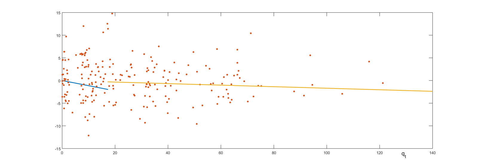
Figure 5: Scatter plot of AR(1) residuals of $y_{t}$ against $q_{t}$ from reconstructed data for US, and true jump equation

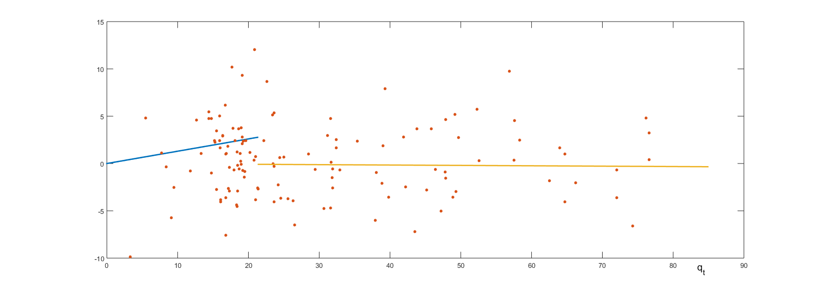
Figure 6: Scatter plot of AR(1) residuals of $y_{t}$ against $q_{t}$ from reconstructed data for Sweden, and true jump equation

References

- [1] Chan, K. S. (1993). “Consistency and limiting distribution of the least squares estimator of a threshold autoregressive model”, The Annals of Statistics, 21, 520-533.
- [2] Chan, K. S., and Tsay, R. S. (1998). “Limiting properties of the least squares estimator of a continuous threshold autoregressive model”, Biometrika, 85, 413-426.
- [3] Chang, Y., Choi, Y., and Park, J. Y. (2017). “A new approach to model regime switching ”, Journal of Econometrics, 196(1), 127-143.
- [4] Feder, P. I. (1975). “On asymptotic distribution theory in segmented regression problems-identified case”, The Annals of Statistics, 3, 49-83.
- [5] Giacomini, R., Dimitris, N. P. and White, H. (2013). “A warp-speed method for conducting Monte Carlo experiments involving bootstrap estimators ”, Econometric Theory, 29, 567-589.
- [6] Hansen, B. E. (1996). “Inference when a nuisance parameter is not identified under the null hypothesis”, Econometrica, 64, 413–430.
- [7] Hansen, B. E. (2000). “Sample splitting and threshold estimation”, Econometrica, 68, 575-603.
- [8] Hansen, B. E. (2017). “Regression kink with an unknown threshold”, Journal of Business and Economic Statistics, 35, 228-240.
- [9] Hansen, B. E., and Seo, B. (2002). Testing for two-regime threshold cointegration in vector error-correction models. Journal of econometrics, 110(2), 293-318.
- [10] Hidalgo, J., Lee, J. and Seo, M. H. (2019). “Robust inference for threshold regression models”, Journal of Econometrics, 210, 291-309.
- [11] Kim, Y. J. and Seo, M. H. (2017). “Is there a jump in the transition?”, Journal of Business & Economic Statistics, 35, 241-249.
- [12] Korostelev, A. (1987). “On minimax estimation of a discontinuous signal”, Theory Probab. Appl., 24-2, 727-730.
- [13] Le Cam, L. (1973). “Convergence of estimates under dimensionality restrictions”, The Annals of Statistics, 1, 38-53.
- [14] Lee, S., Seo, M. H., and Shin, Y. (2011). “Testing for threshold effects in regression models”, Journal of the American Statistical Association, 106, 220-231.
- [15] Lee, S., Seo, M. H., and Shin, Y. (2016). “The lasso for high dimensional regression with a possible change point”, Journal of the Royal Statistical Society: Series B (Statistical Methodology), 78(1), 193-210.
- [16] Lee, S., Liao, Y., Seo, M. H., and Shin, Y. (2018). Oracle estimation of a change point in high-dimensional quantile regression. Journal of the American Statistical Association, 113(523), 1184-1194.
- [17] Lee, S., Liao, Y., Seo, M. H., and Shin, Y. (2021). Factor-driven two-regime regression. The Annals of Statistics, 49(3), 1656-1678.
- [18] Park, J. Y., and Shintani, M. (2016). Testing for a unit root against transitional autoregressive models. International Economic Review, 57(2), 635-664.
- [19] Reinhart, C. M. and Rogoff, K. S. (2010). “Growth in a time of debt”, American Economic Review: Papers and Proceedings, 100, 573-578.
- [20] Seo, M. H. (2006). Bootstrap testing for the null of no cointegration in a threshold vector error correction model. Journal of Econometrics, 134(1), 129-150.
- [21] Seo, M. H. (2008). Unit root test in a threshold autoregression: asymptotic theory and residual-based block bootstrap. Econometric Theory, 24(6), 1699-1716.
- [22] Tong, H. (1990). Non-Linear Time Series: A Dynamical System Approach, New York: Oxford University Press.
- [23] Yu, B. (1997). “Assouad, Fano, and Le Cam”, Research Papers in Probability and Statistics: Festschrift in Honor of Lucien Le Cam, 423-435.