Nonconvex and Nonsmooth Approaches for
Affine Chance-Constrained Stochastic Programs

Abstract

Chance-constrained programs (CCPs) constitute a difficult class of stochastic programs due to its possible nondifferentiability and nonconvexity even with simple linear random functionals. Existing approaches for solving the CCPs mainly deal with convex random functionals within the probability function. In the present paper, we consider two generalizations of the class of chance constraints commonly studied in the literature; one generalization involves probabilities of disjunctive nonconvex functional events and the other generalization involves mixed-signed affine combinations of the resulting probabilities; together, we coin the term affine chance constraint (ACC) system for these generalized chance constraints. Our proposed treatment of such an ACC system involves the fusion of several individually known ideas: (a) parameterized upper and lower approximations of the indicator function in the expectation formulation of probability; (b) external (i.e., fixed) versus internal (i.e., sequential) sampling-based approximation of the expectation operator; (c) constraint penalization as relaxations of feasibility; and (d) convexification of nonconvexity and nondifferentiability via surrogation. The integration of these techniques for solving the affine chance-constrained stochastic program (ACC-SP) is the main contribution of this paper. Indeed, combined together, these ideas lead to several algorithmic strategies with various degrees of practicality and computational efforts for the nonconvex ACC-SP. In an external sampling scheme, a given sample batch (presumably large) is applied to a penalty formulation of a fixed-accuracy approximation of the chance constraints of the problem via their expectation formulation. This results in a sample average approximation scheme, whose almost-sure convergence under a directional derivative condition to a Clarke stationary solution of the expectation constrained-SP as the sample sizes tend to infinity is established. In contrast, sequential sampling, along with surrogation leads to a sequential convex programming based algorithm whose asymptotic convergence for fixed- and diminishing-accuracy approximations of the indicator function can be established under prescribed increments of the sample sizes.

Keywords: chance constraints, nonconvex, nonsmooth, continuous approximations, sampling, exact penalization.

1 Introduction

Chance constrained programs (CCPs) are a class of stochastic optimization problems that restrict the likelihood of undesirable outcomes from a system within a prescribed tolerance. The focus of our study is the following stochastic program with affine chance constraints (ACCs):

$$\begin{array}[]{ll}\displaystyle{\operatornamewithlimits{\mbox{\bf minimize}}_{x\,\in\,X}}&\bar{c}_{0}(x)\,\triangleq\,\mathbb{E}[\,c_{0}(x,\tilde{z})\,]\\[7.22743pt] \mbox{\bf subject to}&\displaystyle{\sum_{\ell=1}^{L}}\,e_{k\ell}\,\mathbb{P}\left(\,{\cal Z}_{\ell}(x,\tilde{z})\,\geq\,0\,\right)\,\leq\,\zeta_{k},\hskip 12.0ptk\,\in\,[\,K\,]\,\triangleq\,\{\,1,\cdots,K\,\},\end{array}$$ (1)

where $X$ is a deterministic constraint set contained in the open set ${\cal O}\subseteq\mathbb{R}^{n}$; $c_{0}\mathrel{\mathop{\ordinarycolon}}{\cal O}\times\Xi\to\mathbb{R}$ is a random functional, $\tilde{z}\mathrel{\mathop{\ordinarycolon}}\Omega\to\Xi$ is a random vector (i.e., a measurable function) defined on the sample space $\Omega$ with values in $\Xi\subseteq\mathbb{R}^{d}$ whose realizations we write without the tilde (i.e., $z=\tilde{z}(\omega)\in\Xi$ for $\omega\in\Omega$); $\mathbb{P}$ is the probability measure defined on the sigma algebra ${\cal F}$ that is generated by subsets of $\Omega$; each $e_{k\ell}$ is a scalar with the signed decomposition $e_{k\ell}=e_{k\ell}^{+}-e_{k\ell}^{-}$, where $e_{k\ell}^{\pm}\geq 0$ are the nonnegative and nonpositive parts of $e_{k\ell}$, respectively; each ${\cal Z}_{\ell}\mathrel{\mathop{\ordinarycolon}}{\cal O}\times\Xi\to\mathbb{R}$ for $\ell\in[L]\triangleq\{\,1,\cdots,L\,\}$ is a bivariate function to be specified in Section 2; and each $\zeta_{k}$ is a given threshold. A special case of (1) is the simplified form (with $\zeta_{k}\in(0,1]$)

$${\operatornamewithlimits{\mbox{\bf minimize}}_{x\in X}}\ \bar{c}_{0}(x)\hskip 12.0pt\mbox{\bf subject to }\ \mathbb{P}({\cal Z}_{k}(x,\tilde{z})\geq 0)\,\leq\,\zeta_{k},\hskip 12.0ptk\in[K],$$ (2)

that is the focus of study in much of the literature on chance-constrained SP [24]. There are two prominent departures of (1) from the traditional case (2): (a) some coefficients $e_{k\ell}$ may be negative, and (b) each functional ${\cal Z}_{\ell}(\bullet,z)$ is nonconvex and nondifferentiable. We postpone the detailed discussion of these features until the next section. Here, we simply note that with these two distinguished features, the formulation (1) covers much broader applications and requires non-traditional treatment with novel theoretical tools and computational methods. The latter constitutes the main contribution of our work.

It is well known that the feasible regions of the CCPs are usually nonconvex even for the linear random functionals and the resulting optimization problems are NP-hard [37, 38]. This nonconvexity partially makes the CCPs one of the most challenging stochastic programs to solve. With over half a century of research, there is an extensive literature on the methodologies and applications of the CCPs. Interested readers are referred to the review papers [1, 21], book chapters [47, 16], the monograph [57], and the lecture notes [24] for detailed discussion.

One direction of developing numerical algorithms for the CCPs focuses on special probability distributions and random functionals, where the multi-dimensional probability function and its subdifferential can be evaluated either directly [25] or efficiently via numerical integration [59, 22]. However, this direct approach does not work for random functionals with general and possibly unknown probability distributions. Numerous methods dealing with general probability distributions include the scenario approximation approach [7, 40], the $p$-efficient point [18, 17] and the sample average approximation (SAA) [55, 36, 42]. In fact, for any random variable $Z$, it holds that

$$\mathbb{P}(Z>0)=\mathbb{E}\left[\,\mathbf{1}_{(0,\infty)}(Z)\,\right]\hskip 12.0pt\mbox{and similarly}\hskip 12.0pt\mathbb{P}(Z\geq 0)=\mathbb{E}\left[\,\mathbf{1}_{[\,0,\infty)}(Z)\,\right],$$ (3)

where $\mathbf{1}_{(0,\infty)}(\bullet)$ is the indicator function of the interval $(0,\infty)$; i.e., $\mathbf{1}_{(0,\infty)}(t)\triangleq\left\{\begin{array}[]{ll}1&\mbox{if $t>0$}\\ 0&\mbox{otherwise;}\end{array}\right.$ Similarly for $\mathbf{1}_{[0,\infty)}(\bullet)$. We call these indicator functions the open and closed Heaviside functions, respectively. The above equalities indicate that the CCPs under discrete or discretized distributions are in principle mixed integer programs (MIPs) that can be solved either by mixed integer algorithms or continuous approximation methods. The former approach leverages auxiliary binary variables and adds the big-M constraints into the lifted feasible set [37]. Strong formulations can also be derived based on specific forms of the random functionals in the constraints. One may consult [30] for a recent survey of the MIP approach for solving the linear CCPs. Although the MIP approach has the advantage of yielding globally optimal solutions, it may not work efficiently in practice when the sample size is large or when nonlinear random functionals are present; its appeal for general distributions may diminish when considering inherent discretization and its effect; the choice of the scalar $M$ is potentially a serious bottleneck. Conservative convex approximations of the CCPs [39] are proposed to resolve this scalability issue. To tighten these convex approximations, recent research [9, 20] has proposed using nonconvex smooth functions as surrogates of the Heaviside functions in the expectation (3); the references [27, 28, 44] further proposed a sample-based scheme using difference-of-convex or other nonconvex smooth functions to deal with general probability distributions.

In this paper, we consider the continuous nonconvex approximation methods to solve the generalized class of CCPs (1). It is worth mentioning that the primary goal of the present paper is neither about proposing new approximation schemes of the CCPs, nor about the comparison of which approximation scheme for the chance constraints is more effective; but rather, we aim to provide a systematic and rigorous mathematical treatment of the nonseparable co-existence of nonconvexity and nondifferentiability in a class of CCPs that extend broadly beyond the settings commonly studied in the literature. Below, we give an overview of the distinguished features of our model and highlight the prevalence of nonconvexity and nondifferentiability:

(a) we treat affine combinations of probability functions in the constraints, which are central to the first-order stochastic dominance of random variables, but cannot be written in the form (2) due to the mixed signs of the coefficients in the combinations;

(b) we approximate the discontinuous Heaviside functions within the expectation formulation of the probability by nonsmooth and nonconvex functions and treat them faithfully; this double “non”-approach enriches the traditional family of convex and/or smooth approximations;

(c) pointwise maximum and/or minimum operators are present within the probabilities; these operators provide algebraic descriptions of conjunctive and/or disjunctive random functional inequalities, and thus logical relations among these inequalities whose probabilities are constrained; and

(d) the resulting random functionals ${\cal Z}_{\ell}(\bullet,\tilde{z})$ within the probabilities are specially structured dc (for difference-of-convex) functions; more precisely, each can be expressed as a difference of two pointwise maxima of finitely many differentiable convex functions.

Mathematical details of this framework and realistic examples of the random functionals are presented in the next section. Throughout this paper, the class of functions in point (d) above plays a central role, although the probability function $\mathbb{P}({\cal Z}_{\ell}(\bullet,\tilde{z})\geq 0)$ may be discontinuous in general, and not of the dc kind even if it is continuous. By a result of [54], piecewise affine functions, which constitute the most basic class of difference-of-convex functions, can be expressed as the difference of two pointwise maxima of finitely many affine functions; see [14, Subsection 4.4.1] for details. Extending this basic result, a related development is the paper [51] which shows that every upper semicontinuous function is the limit of a hypo-convergent sequence of piecewise affine functions. Compared with the linear or convex random functionals considered in the existing literature of CCPs, our overall modeling framework with nonconvex and nondifferentiable random functionals together with probabilities of conjunctive and/or disjunctive random functional inequalities accommodates broader applications in operations research and statistics such as piecewise statistical estimation models [14, 34] and in optimal control such as optimal path planning models [6, 10].

When nonconvexity is present, one needs to be mindful of the fact that globally (or even locally) optimal solutions can rarely be provably computed; thus for practical reasons, it is of paramount importance to design computationally solvable optimization subproblems and to study the computable solutions (instead of minimizers that cannot be computed). In the case of the CCP with nonconvex and nondifferentiabilty features in the constraints, this computational issue becomes more pronounced and challenging. With this in mind, convex programming based sampling methods are desirable for the former task and stationary solutions for the latter.

The locally Lipschitz continuity of the probability distribution function is an important requirement for the applicability of Clarke’s nonsmooth analysis [8]. There are a few results about this property; for instance, in [60, Section 2.6], the random function ${\cal Z}_{\ell}(x,z)$ is separable in its arguments and additional conditions on the vector random variable $\tilde{z}$ are in place; the paper [22] analyzed in detail the subdifferentiability (including the locally Lipschitzian property) of the probability function in Banach space under Gaussian distribution. Even if the Clarke subdifferential of the probability function is well defined, its calculation is usually a nontrivial task except in special cases; thus hindering its practical use. In the event when the probability function fails to be locally Lipschitz continuous, the smoothing-based stochastic approximation methods as in [29] are not applicable. Therefore, instead of a stochastic (sub)gradient-type method, we consider two sampling schemes. One is the external sampling, or SAA [56], where samples of a fixed (presumably large) size are generated to define an empirical optimization problem. The major focus of the external sampling is the statistical analysis of the solution(s) to the empirical optimization problem; such an analysis aims to establish asymptotic properties of the SAA solution(s) in relation to the given expectation problem when the sample size tends to infinity. While computability remains a main concern, the actual computation of the solution is not for the external sampling scheme. In contrast, in an internal, or sequential sampling method [63, 26, 4, 33], samples are gradually accumulated as the iteration proceeds in order to potentially improve the approximation of the expectation operator. By taking advantage of the early stage of the algorithm, the computational cost of subsequent iterations can be reduced. Thus practical computation is an important concern in an internal sampling method.

In order to deal with the expectation constraints and their approximations, we embed the exact penalty approach into the two sampling schemes. Different from the majority of the literature of the exact penalty theory on the asymptotic analysis of the globally optimal solutions whose computation is practically elusive, we focus on the asymptotic behavior of the stationary solutions that are computable by a convex programming based surrogation method. Thus, besides the modeling extensions and the synthesis of various computational schemes, our main contributions pertaining to the sampling methods are twofold:

$\bullet$ The SAA scheme: for the stochastic program (SP) with expectation constraints, we establish the almost sure convergence of the Clarke stationary solutions of penalized SAA subproblems to a Clarke stationary solution of the expectation constrained SP problem when the sample size increases to infinity while the penalty parameter remains finite. Furthermore, we establish that the directional stationary points of the SAA problems are local minima when the random functionals have a “convex-like” property.

$\bullet$ The sequential sampling scheme: we propose a one-loop algorithm that allows for the simultaneous variations of the penalty parameters, either fixed or diminishing approximation accuracy of the Heaviside functions, with the suitable choice of an incremental sequence of sample sizes. This is in contrast to the recent work [61] on solving the nonconvex and nonsmooth CCPs under the fixed sample size and the fixed approximation accuracy, where the convergence of the bundle method is derived for the approximation problem of the CCP; this framework is more restrictive than ours.

The rest of the paper is organized as follows. Section 2 presents the structural assumptions of the bivariate function ${\cal Z}_{\ell}$ and illustrates the sources of the nonsmoothness and nonconvexity by several examples. In Section 3, we provide the approximations of the Heaviside functions composite with the nonconvex random functionals and summarize their properties. Section 4 is devoted to the study of the stationary solutions of the approximated CCPs and their relationship with the local minima. In Section 5, we establish the uniform exact penalty theory for the external sampling scheme of the CCPs in terms of the Clarke stationary solutions. Following that we discuss the internal sampling scheme under both fixed and diminishing parametric approximations of the Heaviside functions in Section 6. The paper ends with a concluding section. Two appendices provide details of some omitted derivations in the main text.

2 Sources of Nonsmoothness and Nonconvexity of the CCP

In this section, we present the structural assumptions of the CCP and provide the sources of nonsmoothness and nonconvexity. Let $X$ be a closed convex set in $\mathbb{R}^{n}$ and $c_{0}\mathrel{\mathop{\ordinarycolon}}\mathbb{R}^{n+d}\to\mathbb{R}$ be a given bivariate Carathéodory function; i.e., $c_{0}(x,\bullet)$ is a measurable function for all $x\in X$ and $c_{0}(\bullet,z)$ is continuous on $X$ for all $z\in\Xi$ with more properties on the latter function to be assumed subsequently. We consider the stochastic program (1) with affine chance constraints (ACCs) at levels $\{\zeta_{k}\}_{k\in[K]}$ with $\zeta_{k}\in\mathbb{R}$ for $k\in[K]$. The following blanket assumption is made throughout the paper:

($\boldsymbol{\cal Z}$) for $\ell=1,\cdots,L$, the bivariate function ${\cal Z}_{\ell}\mathrel{\mathop{\ordinarycolon}}{\cal O}\times\Xi\to\mathbb{R}$ is a specially structured, nondifferentiable, difference-of-convex (dc), function given by: for some positive integers $I_{\ell}$ and $J_{\ell}$,

$${\cal Z}_{\ell}(x,z)\,\triangleq\,\underbrace{\displaystyle{\max_{1\leq i\leq I_{\ell}}}\,g_{i\ell}(x,z)}_{\mbox{denoted $g_{\ell}(x,z)$}}-\underbrace{\displaystyle{\max_{1\leq j\leq J_{\ell}}}\,h_{j\ell}(x,z)}_{\mbox{denoted $h_{\ell}(x,z)$}},$$ (4)

where each $g_{i\ell}\mathrel{\mathop{\ordinarycolon}}{\cal O}\times\Xi\to\mathbb{R}$ and $h_{j\ell}\mathrel{\mathop{\ordinarycolon}}{\cal O}\times\Xi\to\mathbb{R}$ are such that

– the functions $g_{i\ell}(\bullet,z)$ and $h_{j\ell}(\bullet,z)$ are convex, differentiable, and Lipschitz continuous with constant $\mbox{Lip}_{\rm c}(z)>0$ satisfying $\displaystyle{\sup_{z\in\Xi}}\,\mbox{ Lip}_{\rm c}(z)\,<\,\infty$, and $g_{i\ell}(x,\bullet)$ and $h_{j\ell}(x,\bullet)$ are measurable with

$${\max_{1\leq i\leq I_{\ell}}}\,\mathbb{E}\left[\,\left|\,g_{i\ell}(x,\tilde{z})\,\right|\,\right]\,<\,\infty\ \mbox{ and }\ \displaystyle{\max_{1\leq j\leq J_{\ell}}}\,\mathbb{E}\left[\,\left|\,h_{j\ell}(x,\tilde{z})\,\right|\,\right]\,<\,\infty,\hskip 12.0pt\forall\,x\,\in\,X,$$

where $\mathbb{E}$ is the expectation operator; in particular, $g_{i\ell}$ and $h_{j\ell}$ are Carathéodory functions.

Thus, the gradients $\nabla g_{i\ell}(\bullet,z)$ and $\nabla h_{j\ell}(\bullet,z)$ are globally bounded on $X$ uniformly in $z\in\Xi$; that is,

$${\sup_{(x,z)\,\in\,X\times\Xi}}\quad\max\left\{\,\displaystyle{\max_{1\leq i\leq I_{\ell}}}\,\|\,\nabla_{x}g_{i\ell}(x,z)\,\|,\,\displaystyle{\max_{1\leq j\leq J_{\ell}}}\,\|\,\nabla_{x}h_{j\ell}(x,z)\,\|\,\right\}\,<\,\infty.$$

Throughout the paper, the two pointwise maxima in (4) are treated as stated without smoothing. In the following, we explain the role of each component in the constraints of (1) with some examples.

$e_{k\ell}$: affine combinations of probabilities. Mixed-signed affine combinations of probabilities are useful for the modeling of linear relations among probabilities. For example, given a random variable $Z$, a simple inequality like $\mathbb{P}(f_{1}(x,Z)\geq 0)\leq\mathbb{P}(f_{2}(x,Z)\geq 0)$ stipulates that the probability of the event $f_{1}(x,Z)\geq 0$ does not exceed that of the event $f_{2}(x,Z)\geq 0$. Another example of an affine combination of probability functions is the discrete relaxation of the first-order stochastic dominance constraint [57, Chapter 4] in the form of $\mathbb{P}(f_{1}(x,Z)\leq\eta_{1})\leq\mathbb{P}(f_{2}(x,Z)\leq\eta_{2})$ at given levels $\eta_{1}$ and $\eta_{2}$. A third example of a negative coefficient $e_{k\ell}$ is derived from the formula $\mathbb{P}(A\setminus B)=\mathbb{P}(A)-\mathbb{P}(A\cap B)$ to model the probability of event $A$ and the negation of event $B$. To illustrate: suppose that $A$ is the event $f_{1}(x,Z)\geq 0$ and $B$ is the event $f_{2}(x,Z)\geq 0$. Then $A\setminus B$ is the event that $f_{1}(x,Z)\geq 0$ and $f_{2}(x,Z)<0$. Using the formula for the probability of the latter joint event, we obtain

$$\mathbb{P}(f_{1}(x,Z)\geq 0\mbox{ and }f_{2}(x,Z)<0)\,=\,\mathbb{P}(f_{1}(x,Z)\geq 0)-\mathbb{P}(g(x,Z)\geq 0)$$

where $g(x,Z)\,\triangleq\,\min(f_{1}(x,Z),f_{2}(x,Z))$. Lastly, a conditional probability constraint also leads to an affine combination of probabilities. For example,

$$\begin{array}[]{l}\mathbb{P}\left(\,f_{1}(x,Z)\geq 0\ |\ f_{2}(x,Z)\geq 0\,\right)\,\leq\,b\\[7.22743pt] \hskip 12.0pt\Longleftrightarrow\ \mathbb{P}\left[\,\min\left(\,f_{1}(x,Z),\ f_{2}(x,Z)\,\right)\geq 0\,\right]-b\,\mathbb{P}(f_{2}(x,Z)\geq 0)\,\leq\,0\end{array}$$

${\cal Z}_{\ell}$: conjunctive and disjunctive combinations of random inequalities. It is clear that the probability of joint random inequalities $\mathbb{P}(\,f_{i}(x,Z)\geq 0,\;i\in[I]\,)$ is equal to $\mathbb{P}\left(\displaystyle{\min_{1\leq i\leq I}}\,f_{i}(x,Z)\geq 0\right)$. Similarly, one can reformulate the probability of disjunctive functional inequalities using the pointwise max operator. Most generally, combinations $\displaystyle{\bigwedge_{p=1}^{P_{\ell}}}\,\left[\,\widehat{\cal Z}_{\ell p}(x,\tilde{z})\leq 0\,\right]$ and/or $\displaystyle{\bigvee_{q=1}^{Q_{\ell}}}\,\left[\,\widetilde{\cal Z}_{\ell q}(x,\tilde{z})\leq 0\,\right]$ for arbitrary nonnegative integers $P_{\ell}$ and $Q_{\ell}$ can be modelled by pointwise min/max functions to define ${\cal Z}_{\ell}(x,\tilde{z})$. As a simple example, let $f_{1}\mathrel{\mathop{\ordinarycolon}}\mathbb{R}^{n+d}\to\mathbb{R}$ and $f_{2}\mathrel{\mathop{\ordinarycolon}}\mathbb{R}^{n+d}\to\mathbb{R}$ and scalars $\{a_{i}\}_{i=1,2}$ and $\{b_{i}\}_{i=1,2}$ satisfying $a_{1}<b_{1}$ and $a_{2}<b_{2}$ be given. Then,

$$\begin{array}[]{ll}&\mathbb{P}\left(a_{1}\leq f_{1}(x,Z)\leq b_{1}\ \mbox{ or }\ a_{2}\leq f_{2}(x,Z)\leq b_{2}\,\right)\,\leq\,\zeta,\\[5.0pt] \Longleftrightarrow&\mathbb{P}\left(\max\left\{\min\{\,b_{1}-f_{1}(x,Z),\,f_{1}(x,Z)-a_{1}\},\,\min\{\,b_{2}-f_{2}(x,Z),\,f_{2}(x,Z)-a_{2}\}\,\right\}\,\geq\,0\,\right)\,\leq\,\zeta.\end{array}$$

Notice that the composition of maximum and minimum of the above kind is a piecewise linear function and can be written as the difference of two pointwise maxima as follows:

$$\begin{array}[]{l}\max\left\{\,\min\{\,b_{1}-t_{1},t_{1}-a_{1}\},\,\min\{\,b_{2}-t_{2},t_{2}-a_{2}\}\,\right\}\\[5.0pt] \hskip 12.0pt=\,\max\left\{\,-b_{1}+t_{1},\,a_{1}-t_{1},\,-b_{2}+t_{2},\,a_{2}-t_{2}\,\right\}\\[7.22743pt] \hskip 12.0pt-\,\max\left\{\,-b_{1}+t_{1}-b_{2}+t_{2},\,-b_{1}+t_{1}-t_{2}+a_{2},\,-t_{1}+a_{1}-b_{2}+t_{2},\,-t_{1}+a_{1}-t_{2}+a_{2}\,\right\}.\end{array}$$

When each $f_{i}(\bullet,z)$ is of the kind (4), then so is the above difference of two pointwise maxima. More generally, the following result provides the basis to obtain the difference-of-convex representation of a piecewise affine function composite with a function that is the difference of two convex functions each being the pointwise maximum of finitely many convex differentiable functions. While the difference-of-convexity property of such composite functions is addressed by the so-called mixture property in the dc literature (see e.g., [3, 23]), the result shows how the explicit dc representation is defined in terms of the element functions.

Lemma 1.

Let each $\psi_{\ell}(x)=g_{\ell}(x)-h_{\ell}(x)$ with $g_{\ell},h_{\ell}\mathrel{\mathop{\ordinarycolon}}\mathbb{R}^{n}\to\mathbb{R}$ being convex differentiable functions for $\ell=1,\cdots,L$. Let $\varphi\mathrel{\mathop{\ordinarycolon}}\mathbb{R}^{L}\to\mathbb{R}$ be a piecewise affine function written as:

$$\varphi(y)\,=\,\displaystyle{\max_{1\leq i\leq I}}\,\left(\,y^{\top}a^{i}+\alpha_{i}\,\right)-\displaystyle{\max_{1\leq j\leq J}}\,\left(\,y^{\top}b^{\,j}+\beta_{j}\,\right),\hskip 12.0pty\,\in\,\mathbb{R}^{L},$$

for some $L$-vectors $\{a^{i}\}_{i=1}^{I}$ and $\{b^{\,j}\}_{j=1}^{J}$ and scalars $\{\alpha_{i}\}_{i=1}^{I}$ and $\{\beta_{j}\}_{j=1}^{J}$. With $\Psi(x)\triangleq\left(\psi_{\ell}(x)\right)_{\ell=1}^{L}$, the composite function $\varphi\circ\Psi$ can be written as

$$\varphi\circ\Psi(x)\,=\,\displaystyle{\max_{1\leq i\leq\widehat{I}}}\,\widehat{g}_{i}(x)-\displaystyle{\max_{1\leq j\leq\widehat{J}}}\,\widehat{h}_{j}(x)$$

for some positive integers $\widehat{I}$ and $\widehat{J}$ and convex differentiable functions $\widehat{g}_{i}$ and $\widehat{h}_{j}$. A similar expression can be derived when $g_{\ell}$ and $h_{\ell}$ are each the pointwise maximum of finitely many convex differentiable functions.

Proof.

Write $a^{i}_{\ell}=a^{i}_{\ell+}-a^{i}_{\ell-}$ where $a^{i}_{\ell\pm}$ are the nonnegative $(+)$ and nonpositive $(-)$ parts of $a^{i}_{\ell}$, we have

$$\begin{array}[]{rll}\displaystyle{\max_{1\leq i\leq I}}\,\left\{\,\displaystyle{\sum_{\ell=1}^{L}}\,a^{i}_{\ell}\,\left[g_{\ell}(x)-h_{\ell}(x)\,\right]+\alpha_{i}\,\right\}&=&\displaystyle{\max_{1\leq i\leq I}}\,\left\{\,\varphi_{1+}^{\,i}(x)-\varphi_{1-}^{\,i}(x)+\alpha_{i}\,\right\}\\[7.22743pt] \mbox{where}\hskip 12.0pt\varphi_{1\pm}^{\,i}(x)&=&\displaystyle{\sum_{\ell=1}^{L}}\,\left[\,a^{i}_{\ell\pm}\,g_{\ell}(x)+a^{i}_{\ell\mp}\,h_{\ell}(x)\,\right],\end{array}$$

are both convex and differentiable. Thus,

$$\varphi\circ\Psi(x)\,=\,\displaystyle{\max_{1\leq i\leq I}}\,\left(\,\varphi_{1+}^{\,i}(x)-\varphi_{1-}^{\,i}(x)+\alpha_{i}\,\right)-\displaystyle{\max_{1\leq j\leq J}}\,\left(\,\varphi_{2+}^{\,j}(x)-\varphi_{2-}^{\,j}(x)+\beta_{j}\,\right)$$

for some similarly defined convex and differentiable functions $\varphi_{2\pm}^{j}$. Finally, one more manipulation yields

$$\varphi\circ\Psi(x)=\displaystyle{\max_{1\leq i\leq I}}\,\underbrace{\left(\,\widehat{\varphi}_{1+}^{\,i}(x)+\displaystyle{\sum_{i^{\,\prime}\neq i}}\,\varphi_{1-}^{\,i^{\,\prime}}(x)+\displaystyle{\sum_{j=1}^{J}}\,\varphi_{2-}^{\,j}(x)\,\right)}_{\mbox{convex and differentiable in $x$}}-\displaystyle{\max_{1\leq j\leq J}}\,\underbrace{\left(\,\widehat{\varphi}_{2+}^{\,j}(x)+\displaystyle{\sum_{j^{\,\prime}\neq j}}\,\varphi_{2-}^{\,j^{\,\prime}}(x)+\displaystyle{\sum_{i=1}^{I}}\,\varphi_{1-}^{\,i}(x)\,\right)}_{\mbox{convex and differentiable in $x$}},$$

where $\widehat{\varphi}_{1+}^{\,i}(x)\triangleq\varphi_{1+}^{\,i}(x)+\alpha_{i}$ and $\widehat{\varphi}_{2+}^{\,j}(x)\triangleq\varphi_{2+}^{\,j}(x)+\beta_{j}$. Thus the claimed representation of $\varphi\circ\Psi$ follows. We omit the proof of the last statement of the lemma; see Appendix 1. ∎

Consequently, the structure (4) of ${\cal Z}_{\ell}(\bullet,z)$ allows us to model the probability of disjunctive and conjunctive inequalities of random functionals. Probabilities of conjunctive functional inequalities are fairly common in the literature on chance constraints and their treatment using the min function (in our setting) is standard; see e.g. [28, 42, 44]. Nevertheless, it appears that the corresponding literature about probabilities of disjunctive inequalities is scarce; applications of the latter probabilities can be found in optimal path planning to avoid obstacles in robot control [6, 10]. The latter references treat the resulting probability constraint by utilizing the bound $\mathbb{P}(\mbox{A or B})\leq\mathbb{P}(A)+\mathbb{P}(B)$ which provides a very loose approximation of the resulting chance constraint. Thus one contribution of our work is to give a tighter treatment of chance constraints in the presence of conjunctive and disjunctive functional events by modeling them faithfully within the probability operator.

In addition, the piecewise dc structure (4) is central to piecewise statistical models, e.g., in piecewise affine regression [15] and deep neural networks with piecewise affine activation functions [13]. Nonsmooth structures such as these, not only cover more general applications, but also provide computational tractability in terms of directional stationary points. See [15, 43, 35] for algorithms to solve deterministic (composite) optimization problems involving such functions. Furthermore, adding to the large body of literature, the paper [41] has highlighted the fundamental role of the class of difference-of-convex functions in statistics and optimization.

In summary, the class of nonconvex and nondifferentiable random functions ${\cal Z}_{\ell}(\bullet,z)$ given by (4) arises in different ways in statistical modeling and optimization under uncertainty. Their composition with the discontinuous Heaviside functions within the expectation operator makes the exact evaluation of multi-dimensional integrations impossible. Hence, the variational analysis and numerical computation of the overall CCP in (1) are much more involved than a linear or convex random functional that is usually considered in the existing literature, thus necessitating an in-depth treatment that goes beyond a smooth convex programming approach.

3 Computable Approximations of the CCP

In order to design implementable and scalable computational methods to solve the CCP in (1), we consider a family of computationally tractable continuous approximations of the indicator functions of the difference-of-convex type. We denote the feasible set of (1) as

$${X}_{\rm cc}\triangleq\Big{\{}\,x\,\in\,X\ \big{|}\ \displaystyle{\sum_{\ell=1}^{L}}\,e_{k\ell}\,\mathbb{P}\left(\,{\cal Z}_{\ell}(x,\tilde{z})\,\geq\,0\,\right)-\zeta_{k}\,\leq\,0,\hskip 12.0ptk=1,\cdots,K\,\Big{\}}.$$ (5)

One major difficulty of the above constraint is that for each $k\in[K]$, the constraint function

$$x\mapsto\displaystyle{\sum_{\ell=1}^{L}}\,e_{k\ell}\,\mathbb{P}\left(\,{\cal Z}_{\ell}(x,\tilde{z})\,\geq\,0\,\right)\,=\,\displaystyle{\sum_{\ell=1}^{L}}e_{k\ell}\,\mathbb{E}\left[\,{\bf 1}_{[\,0,\infty)}\left(\,{\cal Z}_{\ell}(x,\tilde{z})\,\right)\,\right]$$

is not necessarily continuous. A classical treatment of the continuity of probability functions can be found in [49]; see [60, Section 2.3] for a more recent summary of this continuity issue. Even if such constraint functions are Lipschitz continuous (see [60, Section 2.6] for some conditions), their generalized subdifferentials are impossible to evaluate but their elements can be useful as conceptual targets for computation. Our treatment of the feasible set $X_{\rm cc}$ begins with approximations of the Heaviside functions.

3.1 Approximations of the discontinuous indicator functions

Notice that the function ${\bf 1}_{(\,0,\,\infty)}(\bullet)$ within the expectation function in (3) is lower semicontinuous while the function ${\bf 1}_{[\,0,\,\infty)}(\bullet)$ is upper semicontinuous. In general, there are three steps in obtaining an approximation of these Heaviside functions: i) approximate the indicator functions; ii) parameterize the approximation; and iii) control the parameterization. One way to control the parameterization is to rely on the perspective function and minimize over the parameter, resulting in the conditional value-at-risk approximation of the chance constraint [39]. For complex random functionals, one needs to be careful about the minimization of this parameter over the positive reals and to ensure that a zero value will not be encountered during the solution process. An alternative way to control the parameter is either to take a diminishing sequence of positive parameters and study the limiting process, or to fix a sufficiently small parameter and study the problem with the fixed parameter. We will study both cases in the subsequent sections. As one can expect, the analysis of the former is more challenging.

In what follows, we introduce the unified nonconvex relaxation and restriction of the general affine chance constraints in (1) where the coefficients $\{e_{k\ell}\}$ have mixed signs. Specifically, we employ

$(\boldsymbol{\Theta})$ a convex (thus continuous) function $\widehat{\theta}_{\rm cvx}\mathrel{\mathop{\ordinarycolon}}\mathbb{R}\to\mathbb{R}$ and a concave (thus continuous) function $\widehat{\theta}_{\rm cve}\mathrel{\mathop{\ordinarycolon}}\mathbb{R}\to\mathbb{R}$ satisfying

$$\widehat{\theta}_{\rm cvx}(0)\,=\,0\,=\,\widehat{\theta}_{\rm cve}(0)\hskip 12.0pt\mbox{and}\hskip 12.0pt\widehat{\theta}_{\rm cvx}(1)\,=\,1\,=\,\widehat{\theta}_{\rm cve}(1),$$

and with both functions being increasing in the interval $[0,1]$ and nondecreasing outside.

Truncating these two functions to the range $[\,0,\,1\,]$, we obtain the upper and lower bounds of the two indicator functions ${\bf 1}_{[\,0,\,\infty\,)}(t)$ and ${\bf 1}_{(\,0,\,\infty\,)}(t)$ as follows: for any $(t,\gamma)\,\in\,\mathbb{R}\,\times\,\mathbb{R}_{++}$,

$$\begin{array}[]{lll}\phi_{\rm ub}(t,\gamma)&\triangleq&\min\left\{\,\max\left(\,\widehat{\theta}_{\rm cvx}\left(1+\displaystyle{\frac{t}{\gamma}}\right),\,0\,\right),\,1\,\right\}\\[21.68121pt] &\geq&{\bf 1}_{[\,0,\,\infty\,)}(t)\,\geq\,{\bf 1}_{(\,0,\,\infty\,)}(t)\\[7.22743pt] &\geq&\max\left\{\,\min\left(\,\widehat{\theta}_{\rm cve}\left(\displaystyle{\frac{t}{\gamma}}\right),\,1\,\right),\ 0\,\right\}\,\triangleq\,\phi_{\rm lb}(t,\gamma).\end{array}$$ (6)

One can easily verify that the functions $\phi_{\rm ub}(\bullet,\gamma)$ and $\phi_{\rm lb}(\bullet,\gamma)$ are difference-of-convex functions. When $\widehat{\theta}_{\rm cvx}$ reduces to the identity function, we obtain $\phi_{\rm ub}(t,\gamma)=\min\Big{\{}\max\Big{(}1+\displaystyle\frac{t}{\gamma},\,0\Big{)},\,1\Big{\}}$. This function is used as an approximation of the indicator function in [27, 28], in which the authors made several restrictive assumptions in deriving their analytical results and fixed the scalar $\gamma$ at a prescribed (small) value in their computations. Compared with the conservative convex approximations in [40], the difference-of-convex approximation can provide tighter bounds of the indicator functions.

Illustrated by Figure 1 with $\gamma=1$, the two bivariate functions $\phi_{\rm ub}$ and $\phi_{\rm lb}$ have important properties that we summarize in the result below; these include connections with the Heaviside functions.

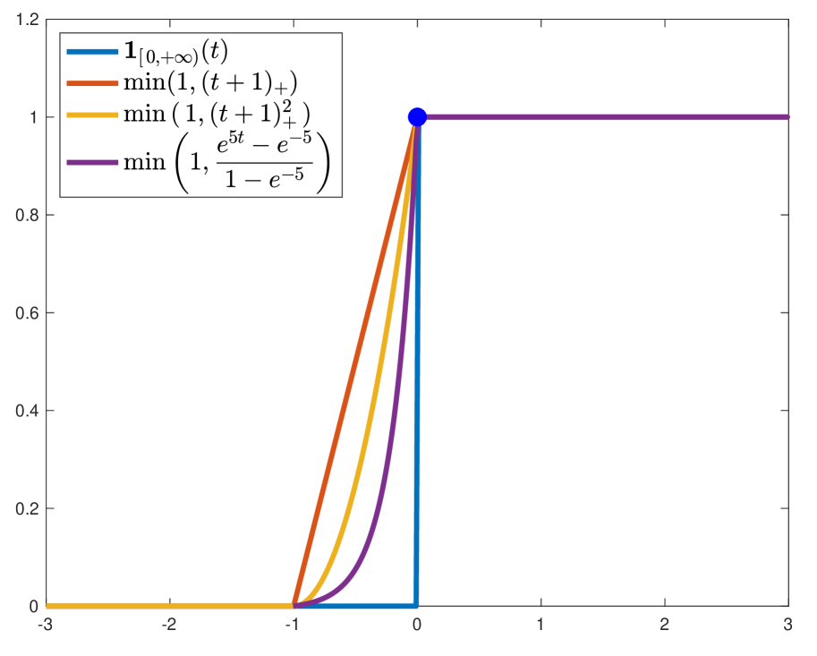
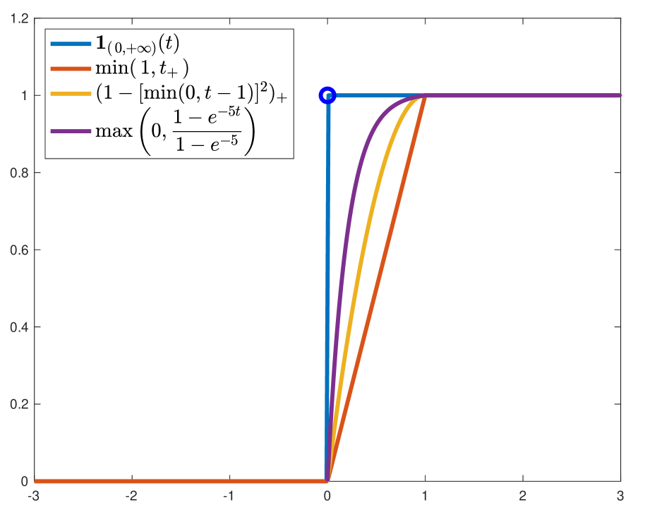
$\phi_{\rm ub}(t,1)$    $\phi_{\rm lb}(t,1)$

Figure 1: Upper bound $\phi_{\rm ub}(t,\gamma)$ and lower bound $\phi_{\rm lb}(t,\gamma)$ of ${\bf 1}_{[0,\infty)}$ and ${\bf 1}_{(0,\infty)}$ with $\gamma=1$.

Proposition 2.

The bivariate functions $\phi_{\rm ub}$ and $\phi_{\rm lb}$ defined above have the following properties:

(a) For any $t\in\mathbb{R}$, $\phi_{\rm ub}(t,\gamma)$ is a nondecreasing function in $\gamma$ on $\mathbb{R}_{++}$ and $\phi_{\rm lb}(t,\gamma)$ is a nonincreasing function in $\gamma$ on $\mathbb{R}_{++}$. Both functions $\phi_{\rm ub}$ and $\phi_{\rm lb}$ are Lipschitz continuous on every compact set $T\times\Gamma\subseteq\mathbb{R}\times\mathbb{R}_{++}$.

(b) The following equalities hold:

$$\begin{array}[]{rll}\mathbf{1}_{[\,0,\infty\,)}(t)&=&\displaystyle{\operatornamewithlimits{\mbox{\bf infimum}}_{\gamma>0}}\ \phi_{\rm ub}(t,\gamma)\,=\,\displaystyle{\operatornamewithlimits{\mbox{\bf limit}}_{\gamma\downarrow 0}}\ \phi_{\rm ub}(t,\gamma),\hskip 12.0pt\forall\,t\,\in\,\mathbb{R}\\[10.84006pt] \mbox{and}\ \mathbf{1}_{(\,0,\infty\,)}(t)&=&\displaystyle{\operatornamewithlimits{\mbox{\bf supremum}}_{\gamma>0}}\ \phi_{\rm lb}(t,\gamma)\,=\displaystyle{\operatornamewithlimits{\mbox{\bf limit}}_{\gamma\downarrow 0}}\ \phi_{\rm lb}(t,\gamma),\hskip 12.0pt\forall\,t\,\in\,\mathbb{R}.\end{array}$$ (7)

Proof.

(a) When $t\geq 0$, $\phi_{\rm ub}(t,\gamma)=1$ for any $\gamma>0$. When $t\leq 0$, $\phi_{\rm ub}(t,\bullet)$ is a nondecreasing function on $\mathbb{R}_{++}$. Thus $\phi_{\rm ub}(t,\bullet)$ is a nondecreasing function on $\mathbb{R}_{++}$ for any $t\in\mathbb{R}$. Similarly, $\phi_{\rm lb}(t,\bullet)$ can be proved to be a nonincreasing function on $\mathbb{R}_{++}$ for any $t\in\mathbb{R}$. To see the Lipschitz continuity of $\phi_{\rm ub}$ and $\phi_{\rm lb}$, it suffices to note that the bivariate function:

$$(\,t,\gamma\,)\,\mapsto\,\displaystyle{\frac{t}{\gamma}},\hskip 12.0pt\gamma\,>\,0$$

is Lipschitz continuous on any such Cartesian set $T\times\Gamma$.

(b) The two equalities in the upper-bound expression in (7) clearly hold when $t\geq 0$ because all three quantities are equal to 1. For $t<0$, we have $1+\displaystyle{\frac{t}{\gamma}}\,<\,0$ for all $\gamma\in(0,-t)$; thus $\displaystyle{\operatornamewithlimits{\mbox{\bf infimum}}_{\gamma>0}}\,\phi_{\rm ub}(t,\gamma)\,=\,\displaystyle{\operatornamewithlimits{\mbox{\bf limit}}_{\gamma\downarrow 0}}\,\phi_{\rm ub}(t,\gamma)\,=\,0$. Similarly, the two equalities in the lower-bound expression clearly hold when $t\leq 0$ because all three quantities are equal to 0. For $t>0$, since $\phi_{\rm lb}(t,\gamma)=1$ for all $\gamma\in(0,t]$, the proof of (7) is complete. ∎

By defining $\phi_{\rm ub}(t,0)\triangleq{\bf 1}_{[0,\infty)}(t)$ and $\phi_{\rm lb}(t,0)\triangleq{\bf 1}_{(0,\infty)}(t)$, Proposition 2 allows us to extend the functions $\phi_{\rm ub}(t,\gamma)$ and $\phi_{\rm lb}(t,\gamma)$ to $\gamma=0$, making the former upper semicontinuous and the latter lower semicontinuous on the closed domain $\mathbb{R}\times\mathbb{R}_{+}$. This is formally stated and proved in the following result.

Proposition 3.

The following limiting inequalities hold for all pairs $(t_{*},\gamma_{*})\in\mathbb{R}\times\mathbb{R}_{+}$:

$$\phi_{\rm ub}(t_{*},\gamma_{*})\,\geq\,\displaystyle{\operatornamewithlimits{\mbox{\bf limsup}}_{(t,\gamma)\to(t_{*},\gamma_{*})}}\ \phi_{\rm ub}(t,\gamma)\,\geq\,\displaystyle{\operatornamewithlimits{\mbox{\bf liminf}}_{(t,\gamma)\to(t_{*},\gamma_{*})}}\ \phi_{\rm lb}(t,\gamma)\,\geq\,\phi_{\rm lb}(t_{*},\gamma_{*}).$$

Proof.

With the definition of $\phi_{\rm ub}$ and $\phi_{\rm lb}$ extended to the entire domain $\mathbb{R}\times\mathbb{R}_{+}$ as described above, the first inequality clearly holds for $t_{*}\geq 0$ and all $\gamma_{*}\geq 0$ because $\phi_{\rm ub}(t_{*},\gamma_{*})=1$ for all such pairs $(t_{*},\gamma_{*})$; see the left curve in Figure 1. Similarly the last inequality holds for $t_{*}\leq 0$ and all $\gamma_{*}\geq 0$ because $\phi_{\rm lb}(t_{*},\gamma_{*})=0$ for all such pairs $(t_{*},\gamma_{*})$; see the right curve in Figure 1. Moreover, these two inequalities clearly hold for $\gamma_{*}>0$ and all $t_{*}$ because $\phi_{\rm ub}$ and $\phi_{\rm lb}$ are both continuous on $\mathbb{R}\times\mathbb{R}_{++}$. To complete the proof, it remains to consider $\gamma_{*}=0$ and show

$$\left[\,\displaystyle{\operatornamewithlimits{\mbox{\bf lim}}_{(t,\gamma)\to(t_{*},0)}}\ \phi_{\rm ub}(t,\gamma)\,=\,0,\ \forall\,t_{*}\,<\,0\,\right]\hskip 12.0pt\mbox{and}\hskip 12.0pt\left[\,\displaystyle{\operatornamewithlimits{\mbox{\bf lim}}_{(t,\gamma)\to(t_{*},0)}}\ \phi_{\rm lb}(t,\gamma)\,=\,1,\ \forall\,t_{*}\,>\,0\,\right].$$

The latter two limits are fairly obvious and no further proof is needed; indeed, it suffices to note that all $t$ near a nonzero $t_{*}$ must have the same sign as $t_{*}$. ∎

The equalities in (7) are deterministic results. With $Z$ being a random variable, we have similar results in probability. In particular, the proposition below shows that the gap between the limits of the outer and inner approximations as $\gamma\downarrow 0$ is $\mathbb{P}(Z=0)$.

Proposition 4.

For any real-valued random variable $Z$, it holds that

$$\begin{array}[]{ll}\mathbb{P}(Z\geq 0)\,=\,\displaystyle{\operatornamewithlimits{\mbox{\bf infimum}}_{\gamma>0}}\,\mathbb{E}\left[\,\phi_{\rm ub}(Z,\gamma)\,\right]\,=\,\displaystyle{\operatornamewithlimits{\mbox{\bf limit}}_{\gamma\downarrow 0}}\,\mathbb{E}\left[\,\phi_{\rm ub}(Z,\gamma)\,\right],\\[14.45377pt] \mathbb{P}(Z>0)\,=\,\displaystyle{\operatornamewithlimits{\mbox{\bf supremum}}_{\gamma>0}}\,\mathbb{E}\left[\,\phi_{\rm lb}(Z,\gamma)\,\right]\,=\,\displaystyle{\operatornamewithlimits{\mbox{\bf limit}}_{\gamma\downarrow 0}}\,\mathbb{E}\left[\,\phi_{\rm lb}(Z,\gamma)\,\right].\end{array}$$

Proof.

From (7),

$$\mathbb{P}(Z\geq 0)=\mathbb{E}\Big{[}\,\mathbf{1}_{[0,\infty)}(Z)\,\Big{]}\,=\,\mathbb{E}\Big{[}\,\displaystyle{\operatornamewithlimits{\mbox{\bf infimum}}_{\gamma>0}}\ \phi_{\rm ub}(Z,\gamma)\,\Big{]}\,=\,\mathbb{E}\Big{[}\,\displaystyle{\operatornamewithlimits{\mbox{\bf limit}}_{\gamma\downarrow 0}}\ \phi_{\rm ub}(Z,\gamma)\,\Big{]}.$$

Since $\phi_{\rm ub}(z,\bullet)$ is a monotonic function on $\mathbb{R}_{++}$, by the Monotone Convergence Theorem, we have

$$\mathbb{P}(Z\geq 0)\,=\,\displaystyle{\operatornamewithlimits{\mbox{\bf infimum}}_{\gamma>0}}\,\mathbb{E}\left[\,\phi_{\rm ub}(Z,\gamma)\,\right]\,=\,\displaystyle{\operatornamewithlimits{\mbox{\bf limit}}_{\gamma\downarrow 0}}\,\mathbb{E}\left[\,\phi_{\rm ub}(Z,\gamma)\,\right].$$

The proof for the two equalities of $\mathbb{P}(Z>0)$ is similar and omitted. ∎

Note that for all $t$ in a compact interval of $\mathbb{R}$, the differences $|\,\phi_{\rm ub/lb}(t,\gamma_{1})-\phi_{\rm ub/lb}(t,\gamma_{2})\,|$ are bounded by a positive multiple of $\left|\,\displaystyle{\frac{1}{\gamma_{1}}}-\displaystyle{\frac{1}{\gamma_{2}}}\,\right|$ for all $\gamma_{1}>\gamma_{2}>0$. In the next result, we derive a similar bound on the expectation of the differences $\mathbb{E}[\,|\,\phi_{\rm ub/lb}(Z,\gamma_{1})-\phi_{\rm ub/lb}(Z,\gamma_{2})\,|\,]$ for a given random variable $Z$; the obtained bounds are the basis for understanding the choice of the scaling parameter in the convergence analysis of the algorithm for solving the ACC-SP (1) when $\gamma\downarrow 0$. To derive these bounds, let $F_{Z}$ be the cumulative distribution function (cdf) of $Z$, and for $\gamma>0$,

$$h_{Z}^{\rm lb}(\gamma)\,\triangleq\,\displaystyle{\frac{1}{\gamma}}\,\displaystyle{\int_{\,0}^{\,\gamma}}\,F_{Z}(t)\,dt\hskip 12.0pt\mbox{and}\hskip 12.0pth_{Z}^{\rm ub}(\gamma)\,\triangleq\,\displaystyle{\frac{1}{\gamma}}\,\displaystyle{\int_{\,-\gamma}^{\,0}}\,F_{Z}(t)\,dt.$$ (8)

These are nonnegative functions with $\displaystyle{\lim_{\gamma\downarrow 0}}\,h_{Z}^{\,\rm ub/lb}(\gamma)=F_{Z}(0)$; moreover, $h_{Z}^{\rm ub/lb}$ are nonincreasing/nondecreasing on $\mathbb{R}_{++}$, respectively. Indeed, we have,

$$\begin{array}[]{lll}(\,h_{Z}^{\rm ub})^{\,\prime}(\gamma)&=&-\displaystyle{\frac{1}{\gamma^{2}}}\,\displaystyle{\int_{\,-\gamma}^{\,0}}\,F_{Z}(t)\,dt+\displaystyle{\frac{1}{\gamma}}\,F_{Z}(-\gamma)\\[14.45377pt] &\leq&-\displaystyle{\frac{1}{\gamma^{2}}}\,\displaystyle{\int_{\,-\gamma}^{\,0}}\,F_{Z}(-\gamma)\,dt+\displaystyle{\frac{1}{\gamma}}\,F_{Z}(-\gamma)\hskip 12.0pt\mbox{because $F_{Z}$ is nondecreasing}\\[14.45377pt] &=&-\displaystyle{\frac{1}{\gamma}}\,F_{Z}(-\gamma)+\displaystyle{\frac{1}{\gamma}}\,F_{Z}(-\gamma)\,=\,0.\end{array}$$

In terms of the functions $h_{Z}^{\,\rm ub/lb}$, we have the following result.

Proposition 5.

Let $\mbox{Lip}_{\theta}$ denote the Lipschitz modulus of $\widehat{\theta}_{\rm cvx/cve}$ on $[0,1]$. For any random variable $Z$, it holds that for any two scalars $\gamma_{1}>\gamma_{2}>0$,

$$\begin{array}[]{lll}0\,\leq\,\mathbb{E}\left[\,\phi_{\rm ub}(Z,\gamma_{1})-\phi_{\rm ub}(Z,\gamma_{2})\,\right]&\leq&\mbox{Lip}_{\theta}\,\left[\,h_{Z}^{\rm ub}(\gamma_{2})-h_{Z}^{\rm ub}(\gamma_{1})\,\right]\\[7.22743pt] 0\,\leq\,\mathbb{E}\left[\,\phi_{\rm lb}(Z,\gamma_{2})-\phi_{\rm lb}(Z,\gamma_{1})\,\right]&\leq&\mbox{Lip}_{\theta}\,\left[\,h_{Z}^{\rm lb}(\gamma_{1})-h_{Z}^{\rm lb}(\gamma_{2})\,\right].\end{array}$$ (9)

Proof.

We prove only the right-hand inequality in (9) for $\phi_{\rm ub}$. We have

$$\begin{array}[]{l}\mathbb{E}\left[\,\phi_{\rm ub}(Z,\gamma_{1})-\phi_{\rm ub}(Z,\gamma_{2})\,\right]\\[7.22743pt] =\,\displaystyle{\int_{\,-\gamma_{1}}^{\,-\gamma_{2}}}\,\widehat{\theta}_{\rm cvx}\left(1+\displaystyle{\frac{t}{\gamma_{1}}}\,\right)\,dF_{Z}(t)+\displaystyle{\int_{\,-\gamma_{2}}^{\,0}}\,\left[\,\widehat{\theta}_{\rm cvx}\left(1+\displaystyle{\frac{t}{\gamma_{1}}}\,\right)-\widehat{\theta}_{\rm cvx}\left(1+\displaystyle{\frac{t}{\gamma_{2}}}\,\right)\,\right]dF_{Z}(t)\\[14.45377pt] \leq\,\mbox{Lip}_{\theta}\,\left[\,\displaystyle{\int_{\,-\gamma_{1}}^{\,-\gamma_{2}}}\,\left|\,1+\displaystyle{\frac{t}{\gamma_{1}}}\,\right|\,dF_{Z}(t)+\displaystyle{\int_{\,-\gamma_{2}}^{\,0}}\,\left(\,\displaystyle{\frac{1}{\gamma_{2}}}-\displaystyle{\frac{1}{\gamma_{1}}}\,\right)\,|\,t\,|\,dF_{Z}(t)\,\right].\end{array}$$

Integration by parts yields

$$\begin{array}[]{lll}\displaystyle{\int_{\,-\gamma_{1}}^{\,-\gamma_{2}}}\,\left|\,1+\displaystyle{\frac{t}{\gamma_{1}}}\,\right|\,dF_{Z}(t)&=&\displaystyle{\int_{\,-\gamma_{1}}^{\,-\gamma_{2}}}\,\left(\,1+\displaystyle{\frac{t}{\gamma_{1}}}\,\right)\,dF_{Z}(t)\\[14.45377pt] &=&\left(\,1-\displaystyle{\frac{\gamma_{2}}{\gamma_{1}}}\,\right)\,F_{Z}(-\gamma_{2})-\displaystyle{\frac{1}{\gamma_{1}}}\,\displaystyle{\int_{\,-\gamma_{1}}^{\,-\gamma_{2}}}\,F_{Z}(t)\,dt\end{array}$$

and

$${\int_{\,-\gamma_{2}}^{\,0}}\,\left(\,\displaystyle{\frac{1}{\gamma_{2}}}-\displaystyle{\frac{1}{\gamma_{1}}}\,\right)\,|\,t\,|\,dF_{Z}(t)\,=\,\left(\,\displaystyle{\frac{1}{\gamma_{2}}}-\displaystyle{\frac{1}{\gamma_{1}}}\,\right)\,\left[\,-\gamma_{2}\,F_{z}(-\gamma_{2})+\displaystyle{\int_{\,-\gamma_{2}}^{\,0}}\,F_{Z}(t)\,dt\,\right].$$

Adding the two terms yields

$$\begin{array}[]{lll}\mathbb{E}\left[\,\phi_{\rm ub}(Z,\gamma_{1})-\phi_{\rm ub}(Z,\gamma_{2})\,\right]&\leq&\mbox{Lip}_{\theta}\,\left[\,-\displaystyle{\frac{1}{\gamma_{1}}}\,\displaystyle{\int_{\,-\gamma_{1}}^{\,-\gamma_{2}}}\,F_{Z}(t)\,dt+\left(\,\displaystyle{\frac{1}{\gamma_{2}}}-\displaystyle{\frac{1}{\gamma_{1}}}\,\right)\,\displaystyle{\int_{\,-\gamma_{2}}^{\,0}}\,F_{Z}(t)\,dt\,\right]\\[14.45377pt] &=&\mbox{Lip}_{\theta}\,\left[\,\displaystyle{\frac{1}{\gamma_{2}}}\,\displaystyle{\int_{\,-\gamma_{2}}^{\,0}}\,F_{Z}(t)\,dt-\displaystyle{\frac{1}{\gamma_{1}}}\,\displaystyle{\int_{\,-\gamma_{1}}^{\,0}}\,F_{Z}(t)\,dt\,\right],\end{array}$$

which is the desired bound. ∎

3.2 Approximation of the chance-constrained set $X_{\rm cc}$

In the following, we discuss the continuous approximation of the chance constraints in (5) via the upper and lower approximations of the Heaviside functions provided in the last subsection. Recalling the signed decomposition $e_{k\ell}=e_{k\ell}^{\,\,+}-e_{k\ell}^{\,\,-}$, we have

$${\sum_{\ell=1}^{L}}\,e_{k\ell}\,\mathbb{P}\left(\,{\cal Z}_{\ell}(x,\tilde{z})\,\geq\,0\,\right)\,=\,\displaystyle{\sum_{\ell=1}^{L}}\,\left(\,e_{k\ell}^{\,\,+}-e_{k\ell}^{\,\,-}\,\right)\,\mathbb{P}\left(\,{\cal Z}_{\ell}(x,\tilde{z})\,\geq\,0\,\right).$$

To proceed, we denote, for any $x\in X$ and any $\gamma>0$,

$$\left\{\begin{array}[]{l}\bar{c}_{k}^{\,\rm rlx}(x;\gamma)\,\triangleq\,\mathbb{E}\left[\,c_{k}^{\,\rm rlx}(x,\tilde{z};\gamma)\,\triangleq\,\displaystyle{\sum_{\ell=1}^{L}}\,\left(\,\underbrace{e_{k\ell}^{+}\,\phi_{\rm lb}({\cal Z}_{\ell}(x,\tilde{z}),\gamma)-e_{k\ell}^{-}\,\phi_{\rm ub}({\cal Z}_{\ell}(x,\tilde{z}),\gamma)}_{\mbox{denoted by $c_{k\ell}^{\,\rm rlx}(x,\tilde{z};\gamma)$}}\,\right)\,\right]\\[32.52127pt] \bar{c}_{k}^{\,\rm rst}(x;\gamma)\,\triangleq\,\mathbb{E}\left[\,c_{k}^{\,\rm rst}(x,\tilde{z};\gamma)\,\triangleq\,\displaystyle{\sum_{\ell=1}^{L}}\,\left(\,\underbrace{e_{k\ell}^{+}\,\phi_{\rm ub}({\cal Z}_{\ell}(x,\tilde{z}),\gamma)-e_{k\ell}^{-}\,\phi_{\rm lb}({\cal Z}_{\ell}(x,\tilde{z}),\gamma)}_{\mbox{denoted by $c_{k\ell}^{\,\rm rst}(x,\tilde{z};\gamma)$}}\,\right)\,\right]\end{array}\right.$$ (10)

and

$$\left\{\begin{array}[]{ll}\overline{X}_{\rm rlx}(\gamma)\,\triangleq\,\left\{\,x\in X\ \big{|}\ \bar{c}_{k}^{\,\rm rlx}(x;\gamma)-\zeta_{k}\,\leq\,0,\hskip 12.0ptk\,\in\,[\,K\,]\,\right\}\\[10.84006pt] \overline{X}_{\rm rst}(\gamma)\,\triangleq\,\left\{\,x\in X\ \big{|}\ \bar{c}_{k}^{\,\rm rst}(x;\gamma)-\zeta_{k}\,\leq\,0,\hskip 12.0ptk\,\in\,[\,K\,]\,\right\}.\end{array}\right.$$ (11)

It then follows by Proposition 2 that for any $\gamma>0$,

$$\bar{c}_{k}^{\rm\,rlx}(x;\gamma)\,\leq\,\displaystyle{\sum_{\ell=1}^{L}}\,e_{k\ell}\,\mathbb{P}\left(\,{\cal Z}_{\ell}(x,\tilde{z})\,\geq\,0\,\right)\,\leq\,\bar{c}_{k}^{\rm\,rst}(x;\gamma)\hskip 12.0pt\mbox{and}\hskip 12.0pt\overline{X}_{\rm rst}(\gamma)\subseteq X_{\rm cc}\subseteq\overline{X}_{\rm rlx}(\gamma).$$

The set inclusions show that for any $\gamma>0$, the set $\overline{X}_{\rm rst}(\gamma)$ yields a more restrictive feasible region compared with the set $X_{\rm cc}$ of the original chance constraints while $\overline{X}_{\rm rlx}(\gamma)$ is a relaxation of the latter set. This explains the scripts “rst” and “rlx” in the above notations, which stand for “restricted” and “relaxed”, respectively. With each ${\cal Z}_{\ell}$ given by assumption ($\boldsymbol{\cal Z}$), the sets $\overline{X}_{\rm rst}(\gamma)$ and $\overline{X}_{\rm rlx}(\gamma)$ are closed. However, with the definition of the limit of set-valued mappings in [53, Chapters 4 and 5], the limits of these two sets when $\gamma\downarrow 0$ may not be equal to $X_{\rm cc}$ in general. In order to derive their respective limits, we further define

$$\left\{\begin{array}[]{l}\bar{c}_{k}^{\,\rm rlx}(x)\,\triangleq\,\displaystyle{\sum_{\ell=1}^{L}}\,\Big{(}\,e_{k\ell}^{+}\,\mathbb{P}({\cal Z}_{\ell}(x,\tilde{z})>0)-e_{k\ell}^{-}\,\mathbb{P}({\cal Z}_{\ell}(x,\tilde{z})\geq 0)\,\Big{)}\\[14.45377pt] \bar{c}_{k}^{\,\rm rst}(x)\,\triangleq\,\displaystyle{\sum_{\ell=1}^{L}}\,\Big{(}\,e_{k\ell}^{+}\,\mathbb{P}({\cal Z}_{\ell}(x,\tilde{z})\geq 0)-e_{k\ell}^{-}\,\mathbb{P}({\cal Z}_{\ell}(x,\tilde{z})>0)\,\Big{)}\end{array}\right.$$ (12)

and

$$\left\{\begin{array}[]{ll}\overline{X}_{\rm rlx}\,\triangleq\,\left\{\,x\in X\ \big{|}\ \bar{c}_{k}^{\,\rm rlx}(x)-\zeta_{k}\,\leq\,0,\hskip 12.0ptk\,\in\,[\,K\,]\,\right\}\\[10.84006pt] \overline{X}_{\rm rst}\,\triangleq\,\left\{\,x\in X\ \big{|}\ \bar{c}_{k}^{\,\rm rst}(x)-\zeta_{k}\,\leq\,0,\hskip 12.0ptk\,\in\,[\,K\,]\,\right\}.\end{array}\right.$$ (13)

Based on Proposition 5, we can given the following error of the restricted/relaxed approximations of the affine constraint functions.

Proposition 6.

For any two scalars $\gamma_{1}>\gamma_{2}>0$, it holds that for all $x\in X$,

$$\begin{array}[]{lll}\left|\,\bar{c}_{k}^{\,\rm rst/rlx}(x;\gamma_{1})-\bar{c}_{k}^{\,\rm rst/rlx}(x;\gamma_{2})\,\right|\\[7.22743pt] \leq\,{\mbox{Lip}_{\theta}}\,\displaystyle{\sum_{\ell=1}^{L}}\ |\,e_{k\ell}\,|\ \max\left(\,h_{{\cal Z}_{\ell}(x,\bullet)}^{\rm ub}(\gamma_{2})-h_{{\cal Z}_{\ell}(x,\bullet)}^{\rm ub}(\gamma_{1}),\ \,h_{{\cal Z}_{\ell}(x,\bullet)}^{\rm lb}(\gamma_{1})-h_{{\cal Z}_{\ell}(x,\bullet)}^{\rm lb}(\gamma_{2})\,\right).\end{array}$$

Proof.

We prove only the inequality for the restricted function. But this is fairly easy because

$$\bar{c}_{k}^{\,\rm rst}(x;\gamma_{1})-\bar{c}_{k}^{\,\rm rst}(x;\gamma_{2})\,=\,\displaystyle{\sum_{\ell=1}^{L}}\,\mathbb{E}\left[\,\begin{array}[]{l}e_{k\ell}^{+}\,\left[\,\phi_{\rm ub}({\cal Z}_{\ell}(x,\tilde{z}),\gamma_{1})-\phi_{\rm ub}({\cal Z}_{\ell}(x,\tilde{z}),\gamma_{2})\,\right]\ -\\[10.84006pt] e_{k\ell}^{-}\,\left[\,\phi_{\rm lb}({\cal Z}_{\ell}(x,\tilde{z}),\gamma_{1})-\phi_{\rm lb}({\cal Z}_{\ell}(x,\tilde{z}),\gamma_{2})\,\right]\end{array}\right];$$

the desired inequality then follows readily from (9). ∎

The proposition below summarizes several set-theoretic properties of the two families of closed sets $\{\overline{X}_{\rm rlx}(\gamma)\}_{\gamma>0}$ and $\{\overline{X}_{\rm rst}(\gamma)\}_{\gamma>0}$. The obtained result also provides a sufficient condition under which the limits of these approximating sets coincide with the feasible set $X_{\rm cc}$ of the ACC-SP.

Proposition 7.

The following statements hold:

(i) The family $\left\{\,\overline{X}_{\rm rlx}(\gamma)\,\right\}$ is nondecreasing in $\gamma>0$; the family $\left\{\,\overline{X}_{\rm rst}(\gamma)\,\right\}$ is nonincreasing in $\gamma>0$.

(ii) $\displaystyle{\lim_{\gamma\downarrow 0}}\ \overline{X}_{\rm rst}(\gamma)\,=\,\mbox{cl}\left(\,\displaystyle{\underset{\gamma>0}{\bigcup}}\,\overline{X}_{\rm rst}(\gamma)\,\right)\,\subseteq\,\mbox{cl}(\,\overline{X}_{\rm rst}\,)\,\subseteq\,\mbox{cl}(\,\overline{X}_{\rm rlx}\,)\,=\,\overline{X}_{\rm rlx}\,=\,\displaystyle{\underset{\gamma>0}{\bigcap}}\,\overline{X}_{\rm rlx}(\gamma)\,=\,\displaystyle{\lim_{\gamma\downarrow 0}}\ \overline{X}_{\rm rlx}(\gamma)$.

(iii) If $\mbox{cl}(\,\overline{X}_{\rm rst}\,)\,\subseteq\,\mbox{cl}\left\{\,x\in X\ \left|\right.\ \bar{c}_{k}^{\rm rst}(x)<\zeta_{k},\ \forall\,k\in[K]\,\right\}$, then $\displaystyle{\lim_{\gamma\downarrow 0}}\ \overline{X}_{\rm rst}(\gamma)=\mbox{cl}(\,\overline{X}_{\rm rst}\,)$.

(iv) If $\mathbb{P}({\cal Z}_{\ell}(x,\tilde{z})=0)=0$ for all $\ell=1,\cdots,L$ and all $x\in X$, then $\overline{X}_{\rm rst}=X_{\rm cc}=\overline{X}_{\rm rlx}$. If in addition the assumption in part (iii) holds, then all sets in part (ii) are equal.

Proof.

Since $\phi_{\rm ub}(t,\gamma)$ is a nondecreasing function and $\phi_{\rm lb}(t,\gamma)$ is a nonincreasing function in $\gamma$ for any $t\in\mathbb{R}$, statement (i) is obvious. For statement (ii), the first and last equalities follow from statement (i) and [53, Exercise 4.3]; in particular, the set $\overline{X}_{\rm rlx}$ is closed because $\bar{c}_{k}^{\,\rm rlx}(\bullet)$ is lower semicontinuous. For the other relations, it suffices to prove the inclusion $\displaystyle{\underset{\gamma>0}{\bigcup}}\,\overline{X}_{\rm rst}(\gamma)\,\subseteq\,\overline{X}_{\rm rst}$ and the second-to-last equality. Let $x\in\displaystyle{\underset{\gamma>0}{\bigcup}}\,\overline{X}_{\rm rst}(\gamma)$ be given. Then $x\in\overline{X}_{\rm rst}(\gamma)$ for all $\gamma>0$ sufficiently small because the family $\{\overline{X}_{\rm rst}(\gamma)\}$ is nonincreasing in $\gamma$. Thus, for such $\gamma$, we have

$${\sum_{\ell=1}^{L}}\,\Big{\{}\,e_{k\ell}^{+}\,\mathbb{E}\Big{[}\,\phi_{\rm ub}({\cal Z}_{\ell}(x,\tilde{z}),\gamma)\,\Big{]}-e_{k\ell}^{-}\,\mathbb{E}\Big{[}\,\phi_{\rm lb}({\cal Z}_{\ell}(x,\tilde{z}),\gamma)\,\Big{]}\,\Big{\}}\,\leq\,\zeta_{k}.$$

By letting $\gamma\downarrow 0$ on both sides, with Proposition 4, we deduce $\bar{c}_{k}^{\rm rst}(x)\,\leq\,\zeta_{k}$. Hence $\displaystyle{\underset{\gamma>0}{\bigcup}}\,\overline{X}_{\rm rst}(\gamma)\subseteq\overline{X}_{\rm rst}$. In a similar manner, we can prove $\displaystyle{\underset{\gamma>0}{\bigcap}}\,\overline{X}_{\rm rlx}(\gamma)\subseteq\overline{X}_{\rm rlx}$. Indeed, let $x$ be an element in the left-hand intersection. We then have, for all $\gamma>0$.

$$\bar{c}^{\,\rm rlx}_{k}(x;\gamma)\,=\,\mathbb{E}\left[\,\displaystyle{\sum_{\ell=1}^{L}}\,\left(\,e_{k\ell}^{+}\,\phi_{\rm lb}({\cal Z}_{\ell}(x,\tilde{z}),\gamma)-e_{k\ell}^{-}\,\phi_{\rm ub}({\cal Z}_{\ell}(x,\tilde{z}),\gamma)\,\right)\,\right]\,\leq\,\zeta_{k}.$$

By letting $\gamma\downarrow 0$ on both sides, with Proposition 4 we deduce $\bar{c}_{k}^{\,\rm rlx}(x)\,\leq\,\zeta_{k}$. Thus $x\in\overline{X}_{\rm rlx}$, showing that $\displaystyle{\underset{\gamma>0}{\bigcap}}\,\overline{X}_{\rm rlx}(\gamma)\subseteq\overline{X}_{\rm rlx}$. Conversely, let $x\in\overline{X}_{\rm rlx}$. Since $\mathbb{P}(\mathcal{Z}_{\ell}(x,\tilde{z})>0)\geq\mathbb{E}\left[\,\phi_{\rm lb}({\cal Z}_{\ell}(x,\tilde{z}),\gamma)\,\right]$ and $\mathbb{P}(\mathcal{Z}_{\ell}(x,\tilde{z})\geq 0)\leq\mathbb{E}\left[\,\phi_{\rm ub}({\cal Z}_{\ell}(x,\tilde{z}),\gamma)\,\right]$ for any $\gamma>0$ by Proposition 4, it follows that $\overline{X}_{\rm rlx}\subseteq\overline{X}_{\rm rlx}(\gamma)$ for any $\gamma>0$. Hence, $\overline{X}_{\rm rlx}=\displaystyle{\underset{\gamma>0}{\bigcap}}\,\overline{X}_{\rm rlx}(\gamma)$. To prove (iii), it suffices to note that

$$\left\{\,x\in X\ \left|\right.\ \bar{c}_{k}^{\,\rm rst}(x)<\zeta_{k},\ \forall\,k\,\in\,[K]\,\right\}\subseteq\,\displaystyle{\bigcup_{\gamma>0}}\,\overline{X}_{\rm rst}(\gamma),$$

taking closures on both sides and using the assumption easily establishes the equality of the two sets $\displaystyle{\lim_{\gamma\downarrow 0}}\ \overline{X}_{\rm rst}(\gamma)$ and $\mbox{cl}(\,\overline{X}_{\rm rst}\,)$. Finally, to prove (iv), note that

$$\begin{array}[]{lll}\overline{c}_{k}^{\,\rm rlx}(x)&=&\displaystyle{\sum_{\ell=1}^{L}}\,e_{k\ell}\,\mathbb{P}({\cal Z}_{\ell}(x,\tilde{z})>0)-\displaystyle{\sum_{\ell=1}^{L}}\,e_{k\ell}^{-}\,\mathbb{P}({\cal Z}_{\ell}(x,\tilde{z})=0),\\[14.45377pt] \bar{c}_{k}^{\,\rm rst}(x)&=&\displaystyle{\sum_{\ell=1}^{L}}\,e_{k\ell}\,\mathbb{P}({\cal Z}_{\ell}(x,\tilde{z})>0)+\displaystyle{\sum_{\ell=1}^{L}}\,e_{k\ell}^{+}\,\mathbb{P}({\cal Z}_{\ell}(x,\tilde{z})=0).\end{array}$$

Hence the equalities $\overline{X}_{\rm rst}=X_{\rm cc}=\overline{X}_{\rm rlx}$ follow readily under the zero-probability assumption; and so does the last assertion in this part. ∎

Proposition 7 shares much resemblance with [20, Theorem 3.6]. The only difference is that the cited theorem has a blanket assumption (A0), which implies in particular the closedness of the feasible set $X_{\rm cc}$. We drop this assumption until the last part where we equate all the sets. In the following, we provide an example showing that for a closed set $X_{\rm cc}$ (empty set included), strict inclusions between the three sets $\overline{X}_{\rm rst}$, $X_{\rm cc}$ and $\overline{X}_{\rm rlx}$ are possible if there exists $\ell\in[L]$ such that $\mathbb{P}(\mathcal{Z}_{\ell}(x,\tilde{z})=0)\neq 0$ for some $x$.

Example 8.

Consider the set ${X}_{\rm cc}=\left\{\,x\,\in\,\mathbb{R}\,\mathrel{\mathop{\ordinarycolon}}\,e\,\mathbb{P}(x\,Z\,\geq\,0\,)\,\leq\,\zeta\,\right\}$, where $Z$ is a Bernoulli random variable such that $\mathbb{P}(Z=1)=\mathbb{P}(Z=-1)=1/2$. Then with $e=1$ and $\zeta=0.1$, we have $X_{\rm cc}=\overline{X}_{\rm rst}=\emptyset$ while $\overline{X}_{\rm rlx}=\{0\}$. With $e=-1$ and $\zeta=-0.6$, we have $X_{\rm cc}=\overline{X}_{\rm rlx}=\{0\}$ while $\overline{X}_{\rm rst}=\emptyset$. $\Box$

To end the section, it would be useful to summarize the notations for the constraint functions used throughout the paper. Absence of the scalar $\gamma$, the notations for the objective function are similar.

Notations for constraint functions (similar notations for the objective function) I. Plain: (3 arguments) for the defining functions of the problems $\bullet$ $c_{k\ell}^{\,\rm rlx/rst}(x,z;\gamma)$ defined in (10); — superscripts rlx/rst are omitted in general discussion; e.g. $c_{k}(x,z;\gamma)\triangleq\displaystyle{\sum_{\ell=1}^{L}}\,c_{k\ell}(x,z;\gamma)$ in Sections 4 and 6; — the scalar $\gamma$ is fixed and thus omitted in Section 5 II. bar: for expectation (2 arguments) and probability (1 argument) $\bullet$ $\bar{c}_{k}^{\,\rm rlx/rst}(x;\gamma)\,\triangleq\,\mathbb{E}\left[\,\displaystyle{\sum_{\ell=1}^{L}}\,c_{k\ell}^{\,\rm rlx/rst}(x,\tilde{z};\gamma)\,\right]$ along with the associated sets $\overline{X}_{\rm rlx/rst}(\gamma)$; $\bullet$ $\bar{c}_{k\ell}^{\,\rm rlx/rst}(x)$ defined in (12) along with the associated sets $\overline{X}_{\rm rlx/rst}$; III. hat: (4 arguments) for surrogation used in Section 6 $\bullet$ $\widehat{c}_{k}(\bullet,z;\gamma;\bar{x})$, derived from the surrogation $\widehat{c}_{k\ell}(\bullet,z;\gamma;\bar{x})$ of the summands $c_{k\ell}(\bullet,z;\gamma)$ at $\bar{x}$; — superscripts rlx/rst used when referred to the relaxed/restricted problems; IV. tilde: (3 arguments) for limiting function in convergence analysis of diminishing $\gamma_{\nu}$ $\bullet$ $\widetilde{c}_{k}(x,z;\bar{x})$ used in Subsection 6.2.2.

4 The Expectation Constrained SP

In this section, we start by considering the following abstract stochastic program without referring to the detailed structure of the constraint functions: for given positive integers $K$ and $L$ and a parameter $\gamma>0$,

$$\begin{array}[]{ll}\displaystyle{\operatornamewithlimits{\mbox{\bf minimize}}_{x\in X}}&\bar{c}_{0}(x)\,\triangleq\,\mathbb{E}\left[\,c_{0}(x,\tilde{z})\,\right]\\[7.22743pt] \mbox{\bf subject to}&\bar{c}_{k}(x;\gamma)\,\triangleq\,\mathbb{E}\left[\,\underbrace{\displaystyle{\sum_{\ell=1}^{L}}\,c_{k\ell}(x,\tilde{z};\gamma)}_{\mbox{denoted $c_{k}(x,\tilde{z};\gamma)$}}\,\right]\,\leq\,\zeta_{k},\hskip 12.0ptk\,=\,1,\cdots,K.\end{array}$$ (14)

Subsequently, we will specialize the constraint functions to those in the sets $\overline{X}_{\rm rlx}(\gamma)$ and $\overline{X}_{\rm rst}(\gamma)$ that are defined in (11) and apply the results to the following two problems:

$\bullet$ Relaxed Problem:

$$\begin{array}[]{ll}\displaystyle{\operatornamewithlimits{\mbox{\bf minimize}}_{x\,\in\,\overline{X}_{\rm rlx}(\gamma)}}&\mathbb{E}[\,c_{0}(x,\tilde{z})\,].\end{array}$$ (15)

$\bullet$ Restricted Problem:

$$\begin{array}[]{ll}\displaystyle{\operatornamewithlimits{\mbox{\bf minimize}}_{x\,\in\,\overline{X}_{\rm rst}(\gamma)}}&\mathbb{E}[\,c_{0}(x,\tilde{z})\,].\end{array}$$ (16)

Abstracting assumption ($\boldsymbol{\cal Z}$) in Section 2 for the functionals $\{{\cal Z}_{\ell}\}_{\ell\in[L]}$ and assumption ($\boldsymbol{\Theta}$) for the functions $\widehat{\theta}_{\rm rst/rlx}$, we make the following blanket assumptions on the functions in (14). Thus the assumptions below on $c_{k\ell}(\bullet,\bullet;\gamma)$ are satisfied for $c_{k\ell}^{\rm rlx}(\bullet,\bullet;\gamma)$ and $c_{k\ell}^{\rm rst}(\bullet,\bullet;\gamma)$ that define the feasible sets in problems (15) and (16).

Blanket Assumptions on (14) $\bullet$ $X\subseteq\mathbb{R}^{n}$ is a closed convex set (and is a polytope starting from Propostion 17) and the objective function $c_{0}(\bullet,z)$ is nonnegative on $X$ for all $z\in\Xi$; this holds for instance when $c_{0}(\bullet,\bullet)$ has a known lower bound on $X\times\Xi$; $\bullet$ Objective (A_o): the function $c_{0}(\bullet,z)$ is directionally differentiable and globally Lipschitz continuous with a Lipschitz constant $\mbox{Lip}_{0}(z)>0$ satisfying $\mathbb{E}\left[\,\mbox{Lip}_{0}(\tilde{z})\,\right]<\infty$. This implies that the expectation function $\bar{c}_{0}(x)$ is directionally differentiable and globally Lipschitz continuous; moreover its directional derivative $\bar{c}_{0}^{\,\prime}(\bar{x};v)=\mathbb{E}\left[c_{0}(\bullet,\tilde{z})^{\prime}(\bar{x};v)\right]$ for all $(\bar{x},v)\in X\times\mathbb{R}^{n}$; see [57, Theorem 7.44] for the latter directional derivative formula. $\bullet$ Constraint (A_c): there exist integrable functions $\mbox{Lip}_{\rm c}(\bullet)$ and $\widehat{\mbox{Lip}}_{\rm c}(\bullet)$ both mapping $\Xi$ into $\mathbb{R}_{++}$ and a probability-one set $\Xi_{\rm c}$ such that $\displaystyle{\sup_{z\in\Xi_{\rm c}}}\,\mbox{Lip}_{\rm c}(z)<\infty$ and — Uniform Lipschitz continuity in $x$: for all tuples $(\,x^{1},x^{2},z,\gamma\,)\,\in\,X\,\times\,X\,\times\,\Xi_{\rm c}\,\times\,\mathbb{R}_{++}$, $$\left|\,c_{k\ell}(x^{1},z;\gamma)-c_{k\ell}(x^{2},z;\gamma)\,\right|\,\leq\,\displaystyle{\frac{\mbox{Lip}_{\rm c}(z)}{\gamma}}\,\|\,x^{1}-x^{2}\,\|,\hskip 12.0pt\forall\,(\,k,\ell\,)\,\in\,[\,K\,]\,\times\,[\,L\,];$$ (17) — Uniform Lipschitz continuity in $1/\gamma$: for all tuples $(\,x,z,\gamma_{1},\gamma_{2}\,)\,\in\,X\,\times\,\Xi_{\rm c}\,\,\times\,\mathbb{R}_{++}^{2}$, $$\left|\,c_{k\ell}(x,z;\gamma_{1})-c_{k\ell}(x,z;\gamma_{2})\,\right|\,\leq\,\widehat{\mbox{Lip}}_{\rm c}(z)\,\left[\,1+\|\,x\,\|\,\right]\,\left|\,\displaystyle{\frac{1}{\gamma_{1}}}-\displaystyle{\frac{1}{\gamma_{2}}}\,\right|,\hskip 12.0pt\forall\,(k,\ell\,)\,\in\,[\,K\,]\times[\,L\,].$$ Remark: As it turns out, the latter Lipschitz continuity in $1/\gamma$ is not useful for the analysis; nevertheless we include it for completeness and also in contrast to the former Lipschitz continuity in $x$. The noteworthy point of (17) is that $\gamma$ appears in the denominator; this feature carries over to a later assumption about the growth of the “Rademacher average” of the random variables $c_{k}(x,\bullet;\gamma)\triangleq\displaystyle{\sum_{\ell=1}^{L}}\,c_{k\ell}(x,\bullet;\gamma)$. $\bullet$ Interchangeability of directional derivatives (I_dd): each expectation function $\bar{c}_{k}(\bullet\,;\gamma)$ is directionally differentiable with directional derivative given by $$\bar{c}_{k}(\bullet;\gamma)^{\,\prime}(\bar{x};v)\,=\,\displaystyle{\sum_{\ell=1}^{L}}\,\mathbb{E}\left[\,c_{k\ell}(\bullet,\tilde{z};\gamma)^{\,\prime}(\bar{x};v)\,\right],\;\,\forall\,(\bar{x},\gamma;v)\,\in\,X\times\mathbb{R}_{++}\times\mathbb{R}^{n}\;\mbox{and all $k\in[K]$}.$$

Associated with the expectation problem (14) is its discretized/empirical (or sample average approximated) version corresponding to a given family of samples $Z^{N}\,\triangleq\,\{z^{s}\}_{s=1}^{N}\,\subseteq\,\mathbb{R}^{d}$ for some positive integer $N$ that are realizations of the nominal random variable $\tilde{z}$:

$$\begin{array}[]{ll}\displaystyle{\operatornamewithlimits{\mbox{\bf minimize}}_{x\in X}}&c_{0}^{N}(x)\,\triangleq\,\displaystyle{\frac{1}{N}}\,\displaystyle{\sum_{s=1}^{N}}\ c_{0}(x,z^{s})\\[7.22743pt] \mbox{\bf subject to}&c_{k}^{N}(x;\gamma)\,\triangleq\,\displaystyle{\frac{1}{N}}\,\displaystyle{\sum_{s=1}^{N}}\ \displaystyle{\sum_{\ell=1}^{L}}\,c_{k\ell}(x,z^{s};\gamma)\,\leq\,\zeta_{k},\hskip 12.0ptk=1,\cdots,K,\end{array}$$ (18)

whose feasible set we denote $\overline{X}(Z^{N};\gamma)$. This empirical problem is the key computational workhorse for solving the expectation problem (14).

4.1 Preliminaries on stationarity

In order to define the stationary solutions of problem (14) and its empirical counterpart (18), we first review some concepts in nonsmooth analysis [50, 14]. By definition, a function $\phi\mathrel{\mathop{\ordinarycolon}}{\cal O}\subseteq\mathbb{R}^{n}\to\mathbb{R}$ defined on the open set ${\cal O}$ is B(ouligand)-differentiable at $\bar{x}\in{\cal O}$ if $\phi$ is locally Lipschitz continuous and directionally differentiable at $\bar{x}$; the latter means that the (elementary) one-sided directional derivative:

$$\phi^{\prime}(\bar{x};v)\,\triangleq\,\displaystyle{\lim_{\tau\downarrow 0}}\,\displaystyle{\frac{\phi(\bar{x}+\tau v)-\phi(\bar{x})}{\tau}}$$

exists for all directions $v\in\mathbb{R}^{n}$. By the locally Lipschitz continuity of $\phi$ at $\bar{x}$, we have [14, Proposition 4.4.1]

$${\lim_{\bar{x}\neq x\to\bar{x}}}\,\displaystyle{\frac{\phi(x)-\phi(\bar{x})-\phi^{\prime}(\bar{x};x-\bar{x})}{\|\,x-\bar{x}\,\|}\,=\,0.}$$ (19)

The directional derivative $\phi^{\prime}(\bar{x};v)$ is in contrast to the Clarke directional derivative

$$\phi^{\circ}(\bar{x};v)\,\triangleq\,\displaystyle{\limsup_{\begin{subarray}{c}x\to\bar{x}\\ \tau\downarrow 0\end{subarray}}}\,\displaystyle{\frac{\phi(x+\tau v)-\phi(x)}{\tau}}\,,\hskip 12.0pt(\bar{x},v)\,\in\,{\cal O}\,\times\,\mathbb{R}^{n},$$

which is always well defined and satisfies $\phi^{\circ}(\bar{x};v)\geq\phi^{\,\prime}(\bar{x};v)$ for any pair $(\bar{x},v)$. If equality holds for all $v\in\mathbb{R}^{n}$ at some $\bar{x}\in{\cal O}$, then we say that $\phi$ is Clarke regular at $\bar{x}$. One key property of the Clarke directional derivative is that it is jointly upper semicontinuous in the base point $\bar{x}\in{\cal O}$ and the direction $v\in\mathbb{R}^{n}$; that is, for every sequence $\{(x^{\nu},v^{\nu})\}$ converging to $(\bar{x},\bar{v})$, it holds that

$${\limsup_{\nu\to\infty}}\,\phi^{\circ}(x^{\nu};v^{\nu})\,\leq\,\phi^{\circ}(\bar{x};\bar{v}).$$ (20)

The Clarke subdifferential of $\phi$ at $\bar{x}$ is defined as the set

$$\partial_{C}\phi(\bar{x})\,\triangleq\,\left\{\,a\,\in\,\mathbb{R}^{n}\,\mathrel{\mathop{\ordinarycolon}}\,\phi^{\circ}(\bar{x};v)\,\geq\,a^{\top}v,\ \forall\,v\,\in\,\mathbb{R}^{n}\,\right\}.$$

In general, we say that a vector $\bar{x}$ is a B-stationary point of a B-differentiable function $f_{0}$ on a closed set $\widehat{X}\subseteq{\cal O}$ if $\bar{x}\in\widehat{X}$ and

$$f_{0}^{\,\prime}(\bar{x};v)\,\geq\,0,\hskip 12.0pt\forall\,v\,\in\,{\cal T}(\bar{x};\widehat{X}),$$ (21)

where ${\cal T}(\bar{x};\widehat{X})$ is the (Bouligand) tangent cone of the set $\widehat{X}$ at $\bar{x}$; by definition, a tangent vector $v$ in this cone is the limit of a sequence $\left\{\,\displaystyle{\frac{x^{\nu}-\bar{x}}{\tau_{\nu}}}\,\right\}$ where $\{x^{\nu}\}\subset\widehat{X}$ is a sequence of vectors converging to $\bar{x}$ and $\{\tau_{\nu}\}$ is a sequence of positive scalars converging to zero. When $\widehat{X}$ is convex, we use the terminology “d(irectional) stationarity” for B-stationarity; in this case, the condition (21) is equivalent to

$$f_{0}^{\,\prime}(\bar{x};x-\bar{x})\,\geq\,0,\hskip 12.0pt\forall\,x\,\in\,\widehat{X}.$$

We say that $\bar{x}$ is a C(larke)-stationary point of $f_{0}$ on $\widehat{X}$ if the directional derivative $f_{0}^{\,\prime}(\bar{x};v)$ in (21) is replaced by the Clarke directional derivative. An important special case is when the set $\widehat{X}$ is defined by B-differentiable constraints intersecting a polyhedron $X$:

$$\widehat{X}\,=\,\displaystyle{\bigcap_{k\,\in\,[\,K\,]}}\,\left\{\,x\,\in\,X\,\mid\,f_{k}(x)\,\leq\,0\,\right\},$$

where each $f_{k}$ is B-differentiable. We may then define the directional derivative based “linearization cone” of $\widehat{X}$ at a given vector $\bar{x}\in\widehat{X}$ as

$${\cal L}(\bar{x};\widehat{X})\,\triangleq\,\displaystyle{\bigcap_{k\in{\cal A}(\bar{x})}}\,\left\{\,v\,\in\,{\cal T}(\bar{x};X)\,\mathrel{\mathop{\ordinarycolon}}\,f_{k}^{\,\prime}(\bar{x};v)\,\leq\,0\,\right\},$$ (22)

where ${\cal A}(\bar{x})\triangleq\left\{\,k\,\mathrel{\mathop{\ordinarycolon}}\,f_{k}(\bar{x})\,=\,0\,\right\}$ is the index set of active constraints at $\bar{x}$. Clearly we have

$$\mbox{cl}\left\{\,v\,\in\,{\cal T}(\bar{x};X)\,\mid\,f_{k}^{\,\prime}(\bar{x};v)<0,\,\,\forall\ k\in{\cal A}(\bar{x})\,\right\}\,\subseteq\,{\cal T}(\bar{x};\widehat{X})\,\subseteq\,{\cal L}(\bar{x};\widehat{X}),$$ (23)

where the first inclusion holds because by the closedness of the tangent cone ${\cal T}(\bar{x};\widehat{X})$, one may take closures on both sides of the inclusion:

$$\left\{\,v\,\in\,{\cal T}(\bar{x};X)\,\mid\,f_{k}^{\,\prime}(\bar{x};v)<0,\,\,\forall\ k\in{\cal A}(\bar{x})\,\right\}\,\subseteq\,{\cal T}(\bar{x};\widehat{X}).$$ (24)

The second inequality in (23) holds because for any sequence $\{x^{\nu}\}\subset\widehat{X}$ converging to $\bar{x}$ and any sequence $\{\tau_{\nu}\}\downarrow 0$ with $\displaystyle{\lim_{\nu\to\infty}}\,\displaystyle{\frac{x^{\nu}-\bar{x}}{\tau_{\nu}}}\,=\,v$, we have, by the B-differentiability of $f_{k}$ at $\bar{x}$,

$$\begin{array}[]{llll}f_{k}^{\,\prime}(\bar{x};v)&=&\displaystyle{\lim_{\nu\to\infty}}\,\displaystyle{\frac{f_{k}(x^{\,\nu})-f_{k}(\bar{x})}{\tau_{\nu}}}&{\mbox{by (\ref{eq:Lip+dd})}}\\[14.45377pt] &\leq&0&{\mbox{for $k\in{\cal A}(\bar{x})$}}.\end{array}$$

Clearly, if ${\cal A}(\bar{x})$ is empty, the cone ${\cal L}(\bar{x};\widehat{X})$ coincides with ${\cal T}(\bar{x};\widehat{X})={\cal T}(\bar{x};X)$; i.e., the intersection operation in (22) is vacuous in this case. This remark applies throughout the paper. In general, we say that the Abadie constraint qualification (ACQ) holds for $\widehat{X}$ at $\bar{x}\in\widehat{X}$ if the last two sets in (23) are equal. A sufficient condition for the ACQ to hold is that the directional Slater constraint qualification holds for $\widehat{X}$ at $\bar{x}\in\widehat{X}$; i.e., if the first and the third sets in (23) are equal. In turn, the latter directional Slater CQ holds if the left-hand set in (24) is nonempty and $f_{k}^{\,\prime}(\bar{x};\bullet)$ is a convex function. A function $f_{k}$ with the latter directional-derivative convexity property has been coined a dd-convex function in [14, Definition 4.3.3].

4.2 Convex-like property: B-stationarity implies locally minimizing

A function $f\mathrel{\mathop{\ordinarycolon}}\mathbb{R}^{n}\to\mathbb{R}$ is said to be convex-like near a vector $\bar{x}$ if there exists a neighborhood ${\cal N}_{\bar{x}}$ of $\bar{x}$ such that

$$f(x)\,\geq\,f(\bar{x})+f^{\,\prime}(\bar{x};x-\bar{x}),\hskip 12.0pt\forall\,x\,\in\,{\cal N}_{\bar{x}}.$$

It is clear that the class of convex-like functions near a fixed vector is closed under nonnegative addition. The fundamental role of this property for nonconvex functions was first discussed in [11, Proposition 4.1], which we restate in part (ii) of the following result.

Proposition 9.

Let $X$ be a polyhedron. Suppose that each $f_{k}$ for $k=0,1,\cdots,K$ is B-differentiable on $\mathbb{R}^{n}$. Let $\bar{x}\in\widehat{X}$ be arbitrary. The following two statements hold.

(i) If $\bar{x}$ is a local minimizer of $f_{0}$ on $\widehat{X}$, then $\bar{x}$ is a B-stationary point of $f_{0}$ on $\widehat{X}$.

(ii) If $f_{k}$ for $k=0,1,\cdots,K$ are all convex-like near $\bar{x}$, the ACQ holds for $\widehat{X}$ at $\bar{x}$, and $\bar{x}$ is a B-stationary point of $f_{0}$ on $\widehat{X}$, then $\bar{x}$ is a local minimizer of $f_{0}$ on $\widehat{X}$.

Proof.

The first statement is a standard result. To prove (ii), let $x\in\widehat{X}$ be sufficiently near $\bar{x}$ such that the convex-like inequality holds for all functions $f_{k}$. For any $k\in\mathcal{A}(\bar{x})$, it follows that $f_{k}^{\,\prime}(\bar{x};x-\bar{x})\leq f_{k}(x)\leq 0$, and thus, $x-\bar{x}\in{\cal L}(\bar{x};\widehat{X})={\cal T}(\bar{x};\widehat{X})$. By the convex-like inequality for the function $f_{0}$ and the B-stationarity of $\bar{x}$, we have

$$f_{0}(x)\,\geq\,f_{0}(\bar{x})+f_{0}^{\,\prime}(\bar{x};x-\bar{x})\,\geq\,f_{0}(\bar{x}),$$

and thus the claim in (ii) follows. ∎

In what follows, we present a broad class of composite functions that have this property. Let

$$f(x)\,\triangleq\,\varphi\circ\theta\,\circ\,\psi(x),$$ (25)

where $\varphi\mathrel{\mathop{\ordinarycolon}}\mathbb{R}\to\mathbb{R}$ is piecewise affine and nondecreasing; $\theta\mathrel{\mathop{\ordinarycolon}}\mathbb{R}\to\mathbb{R}$ is convex, and $\psi\mathrel{\mathop{\ordinarycolon}}\mathbb{R}^{n}\to\mathbb{R}$ is piecewise affine.

Lemma 10.

The function $f$ given by (25) with properties as described is convex-like near any $\bar{x}\in\mathbb{R}^{n}$.

Proof. The key of the proof is the fact (cf. [11, Proposition 4.1]) that for any piecewise affine (PA) function $H\mathrel{\mathop{\ordinarycolon}}\mathbb{R}^{M}\to\mathbb{R}$ and any $\bar{y}\in\mathbb{R}^{M}$, there exists a neighborhood ${\cal N}_{\bar{y}}$ of $\bar{y}$ such that

$$H(y)\,=\,H(\bar{y})+H^{\,\prime}(\bar{y};y-\bar{y}),\hskip 12.0pt\forall\,y\,\in\,{\cal N}_{\bar{y}}.$$

Applying this result to $\psi$ at $\bar{x}$ and also to $\varphi$ at $\bar{t}\triangleq\theta(\psi(\bar{x}))$, we deduce the existence of a neighborhood ${\cal N}_{\bar{x}}$ of $\bar{x}$ such that

$$\begin{array}[]{lll}\varphi\circ\theta\,\circ\,\psi(x)&=&\varphi(\bar{t})+\varphi^{\,\prime}(\bar{t};\theta(\psi(x))-\theta(\psi(\bar{x})))\hskip 28.90755pt\mbox{by PA property of $\varphi$ at $\bar{t}$}\\[7.22743pt] &\geq&\varphi(\bar{t})+\varphi^{\,\prime}(\bar{t};\theta^{\,\prime}(\psi(\bar{x});\psi(x)-\psi(\bar{x})))\ \mbox{by convexity of $\theta$ and $\uparrow$ property of $\varphi^{\,\prime}(\bar{t};\bullet)$}\\[7.22743pt] &=&\varphi(\bar{t})+\varphi^{\,\prime}(\bar{t};\theta^{\,\prime}(\psi(\bar{x});\psi^{\,\prime}(\bar{x};x-\bar{x})))\hskip 25.29494pt\mbox{by PA property of $\psi$ at $\bar{x}$}\\[7.22743pt] &=&\varphi(\theta(\psi(\bar{x})))+\left(\,\varphi\circ\theta\,\circ\,\psi\,\right)^{\,\prime}(\bar{x};x-\bar{x})\ \mbox{by the chain rule of the dir.\ derivative.}\hskip 12.0pt\Box\end{array}$$

With the above lemma, we can easily obtain the following corollary of Proposition 9 applied to the empirical problem (18) for a fixed sample batch $Z^{N}=\{z^{s}\}_{s=1}^{N}$ when the problem is derived from the expectation problems (15) and (16) with fixed $\gamma>0$. This requires the functions $c^{\,\rm rst}_{k\ell}(\bullet,z;\gamma)$ and $c^{\,\rm rlx}_{k\ell}(\bullet,z;\gamma)$ to have the composite structure in (25).

Corollary 11.

Let $X$ be a polyhedron and $\gamma>0$ be a fixed but arbitrary scalar. Using the notation in (10), we let each constraint function

$\bullet$ for the restricted problem: $c_{k\ell}(\bullet,z;\gamma)=c_{k\ell}^{\,\rm rst}(\bullet,z;\gamma)$ for all $(k,\ell)\in[K]\times[L]$;

$\bullet$ for the relaxed problem: $c_{k\ell}(\bullet,z;\gamma)=c_{k\ell}^{\,\rm rlx}(\bullet,z;\gamma)$ for all $(k,\ell)\in[K]\times[L]$.

Suppose that $\left\{\,g_{i\ell}(\bullet,z)\,\right\}_{i=1}^{I_{\ell}}$ and $\left\{\,h_{j\ell}(\bullet,z)\,\right\}_{j=1}^{J_{\ell}}$ are all affine functions. Then $c_{k\ell}(\bullet,z;\gamma)$ is convex-like near any $\bar{x}\in X$ for all $(k,\ell)\in[K]\times[L]$, provided that

$\bullet$ for the restricted problem: $\widehat{\theta}_{\rm cvx}$ and $\widehat{\theta}_{\rm cve}$ are convex and concave functions, respectively;

$\bullet$ for the relaxed problem: $\widehat{\theta}_{\rm cvx}$ and $\widehat{\theta}_{\rm cve}$ are piecewise affine (not necessarily convex/concave).

If additionally, the objective function $c_{0}(\bullet,z)$ is convex-like near a B-stationary point $\bar{x}$ of (18) satisfying the ACQ for the feasible set $\overline{X}(Z^{N};\gamma)$, then $\bar{x}$ is a local minimizer of (18).

Proof.

Writing $t_{\ell}\triangleq{\cal Z}_{\ell}(x,z)$, we have, for the restricted problem,

$$c^{{\,\rm rst}}_{k\ell}(x,z;\gamma)\,=\,e_{k\ell}^{+}\min\left\{\,\max\left(\,\widehat{\theta}_{\rm cvx}\left(1+\displaystyle{\frac{t_{\ell}}{\gamma}}\right),\,0\right),\,1\,\right\}+e_{k\ell}^{-}\,\min\left\{\,\max\left(\,-\widehat{\theta}_{\rm cve}\left(\displaystyle{\frac{t_{\ell}}{\gamma}}\right),\,-1\,\right),\,0\,\right\}.$$

By (4), it follows $t_{\ell}$ is a piecewise affine function of $x$ for fixed $z$. Thus $c^{{\,\rm rst}}_{k\ell}(\bullet,z;\gamma)$ is of the kind (25) and the claims hold in this case. For the relaxed problem, we have

$$c^{{\,\rm rlx}}_{k\ell}(x,z;\gamma)\,=\,-e_{k\ell}^{-}\min\left\{\,\max\left(\,\widehat{\theta}_{\rm cvx}\left(1+\displaystyle{\frac{t_{\ell}}{\gamma}}\right),\,0\right),\,1\,\right\}-e_{k\ell}^{+}\,\min\left\{\,\max\left(\,-\widehat{\theta}_{\rm cve}\left(\displaystyle{\frac{t_{\ell}}{\gamma}}\right),\,-1\,\right),\,0\,\right\},$$

which shows that $c^{{\,\rm rlx}}_{k\ell}(\bullet,z;\gamma)$ is the composite of piecewise affine functions, thus is piecewise affine itself. Hence the claims also hold in this case. ∎

4.3 Asymptotic results for $\gamma\downarrow 0$

Based on Proposition 7 that asserts the limits of the approximating sets $\overline{X}_{\rm rlx}(\gamma)$ and $\overline{X}_{\rm rst}(\gamma)$ as $\gamma\downarrow 0$, it is easy to show that under the zero-probability assumption in Proposition 7(iv), any accumulation point of the globally optimal solutions of the relaxed problem (15) as $\gamma\downarrow 0$ must be a globally optimal solution of the original chance-constrained problem (1). Additionally under the condition in Proposition 7(iii), any accumulation point of the globally optimal solutions of the restricted problem (16) as $\gamma\downarrow 0$ must be a globally optimal solution of the original chance-constrained problem (1). However, an accumulation point of (strictly) locally optimal solutions $\{\bar{x}_{\,\rm rst}(\gamma)\}$ of (16) may not be a locally optimal solution of (1) even with the conditions in Proposition 7(iii) and (iv). In the following, we provide an example to illustrate the latter fact. A slightly modified example illustrates an unexpected limit with the relaxed problem.

Example 12.

Consider the problem

$${\operatornamewithlimits{\mbox{\bf minimize}}_{-1\,\leq\,x\,\leq\,1}}\ x\hskip 12.0pt\mbox{\bf subject to }\ \mathbb{P}\left(\,{\color[rgb]{0,0,0}Z-\max(2x,1-2x)\geq 0}\,\right)\,\leq\,\displaystyle{\frac{1}{4}},$$ (26)

where the random variable $Z$ is uniformly distributed on $[\,-1,1\,]$. We can show

$\bullet$ $\mathbb{P}\left(\,Z-\max(2x,1-2x)\,=\,0\,\right)=0$ for $x\in[-1,1]$;

$\bullet$ $\mathbb{P}\left(\,Z-\max(2x,1-2x)\geq 0\,\right)\,=\,\left\{\begin{array}[]{ll}\left(1-2x\right)/2&\mbox{if $x\in\left[\,1/4,\,1/2\,\right)$}\\[7.22743pt] x&\mbox{if $x\in\left[\,0,1/4\,\right)$}\\[7.22743pt] 0&\mbox{if $x\in[-1,0)\,\cup\,\left[\,1/2,\,1\,\right].$}\end{array}\right.$

It follows that the conditions in Proposition 7 (iii) and (iv) both hold. Therefore, ${X}_{\rm cc}=[-1,1]$ and the unique B-stationary point/local minimizer/global minimizer of (26) is $\bar{x}=-1$.

$\bullet$ Let $\widehat{\theta}_{\rm cvx}(t)=t$ in $\phi_{\rm ub}(t,\gamma)$. We have for any $\gamma\in(0,1/2)$,

$$\begin{array}[]{ll}\bar{c}^{\,\rm rst}(x;\gamma)&=\mathbb{E}\left[\,\min\left(\,1,\max\left(\,1+\displaystyle{\frac{1}{\gamma}}\,\left(\,Z-\max(2x,1-2x)\,\right),\,0\,\right)\,\right)\,\right]\\[18.06749pt] &=\mathbb{E}\left[\,1\,\left|\;1+\displaystyle{\frac{1}{\gamma}}\,\left(Z-\max(2x,1-2x)\right)\,\geq 1\right.\right]\times\mathbb{P}\left({Z}-{\max(2x,1-2x)}\geq 0\right)\ +\\[21.68121pt] &\hskip 12.0pt\left(\begin{array}[]{l}\,\mathbb{E}\left[1+\displaystyle{\frac{1}{\gamma}}\,\left(Z-\max(2x,1-2x)\right)\,\left|\;1+\displaystyle{\frac{1}{\gamma}}\,\left(\,Z-\max(2x,1-2x)\,\right)\,\in\,(0,1)\,\right.\right]\\[21.68121pt] \hskip 12.0pt\ \times\,\mathbb{P}\left(-\gamma<Z-\max(2x,1-2x)<0\right)\end{array}\,\right)\\[36.135pt] &=\,\left\{\begin{array}[]{ll}\displaystyle{\frac{(\gamma+2x)^{2}}{4\gamma}}&\mbox{if $x\,\in\,\left[\,-\displaystyle{\frac{\gamma}{2}},\,0\,\right)$}\\[18.06749pt] x+\displaystyle{\frac{\gamma}{4}}&\mbox{if $x\,\in\,\left[\,0,\,\displaystyle{\frac{1}{4}}\,\right)$}\\[18.06749pt] \displaystyle{\frac{1}{2}}\,(1-2x)+\displaystyle{\frac{\gamma}{4}}&\mbox{if $x\,\in\,\left[\,\displaystyle{\frac{1}{4}},\,\displaystyle{\frac{1}{2}}\,\right)$}\\[18.06749pt] \displaystyle{\frac{(\gamma+1-2x)^{2}}{4\gamma}}&\mbox{if $x\,\in\,\left[\,\displaystyle{\frac{1}{2}},\,\displaystyle{\frac{1}{2}(1+\gamma)}\,\right)$}\\[18.06749pt] 0&\mbox{if $x\,\in\,\left[\,-1,\,-\displaystyle{\frac{\gamma}{2}}\,\right)\,\cup\,\left[\,\displaystyle{\frac{1}{2}}\,(1+\gamma),\,1\,\right]$}.\end{array}\right.\end{array}$$

Therefore, $\overline{X}_{\rm rst}(\gamma)=\left[\,-1,\,\displaystyle{\frac{1-\gamma}{4}}\,\right]\,\cup\,\left[\,\displaystyle{\frac{1+\gamma}{4}},\,1\,\right]$ for any $\gamma\in(0,1/2)$. Hence, $\bar{x}_{\rm rst}(\gamma)=\displaystyle{\frac{1+\gamma}{4}}$ is a B-stationary point and a strict local minimizer of (16) for any $\gamma\in(0,1/2)$.

$\bullet$ However, the limit of $\{\bar{x}_{\rm rst}(\gamma)\}$ as $\gamma\downarrow 0$ is $\displaystyle\frac{1}{4}$, which is not a local minimizer of (26).

Alternatively, consider the following slight modification of the problem (26):

$${\operatornamewithlimits{\mbox{\bf minimize}}_{-1\,\leq\,x\,\leq\,1}}\ -\left|\,x-\frac{3}{8}\,\right|\hskip 12.0pt\mbox{\bf subject to }\ \mathbb{P}\left(\,Z-\max(2x,1-2x)\geq 0\,\right)\,\leq\,\displaystyle{\frac{1}{8}}$$ (27)

for the same random variable $Z$. Then $X_{\rm cc}=\left[\,-1,\displaystyle\frac{1}{8}\,\right]\cup\left[\,\displaystyle\frac{3}{8},1\,\right]$ and the local minimizer of the above problem is $\{-1,1\}$. Letting $\widehat{\theta}_{\rm cve}(t)=t$ and omitting the details, we get

$$\begin{array}[]{ll}\bar{c}^{\,\rm rlx}(x;\gamma)&=\,\left\{\begin{array}[]{cl}\displaystyle{\frac{(1-2x)^{2}}{4\gamma}}&\mbox{if $x\,\in\,\left[\,\displaystyle{\frac{1-\gamma}{2}},\,\frac{1}{2}\,\right)$}\\[14.45377pt] \displaystyle{\frac{x^{2}}{\gamma}}&\mbox{if $x\,\in\,\left[\,0,\,\displaystyle{\frac{\gamma}{2}}\,\right)$}\\[14.45377pt] \displaystyle{\frac{2-\gamma}{4}}-x&\mbox{if $x\,\in\,\left[\,\displaystyle{\frac{1}{4}},\,\displaystyle{\frac{1-\gamma}{2}}\,\right)$}\\[14.45377pt] x-\displaystyle{\frac{\gamma}{4}}&\mbox{if $x\,\in\,\left[\,\displaystyle{\frac{\gamma}{2}},\,\displaystyle{\frac{1}{4}}\,\right)$}\\[14.45377pt] 0&\mbox{if $x\,\in\,\left[\,-1,\,0\,\right)\,\cup\,\left[\,\displaystyle{\frac{1}{2}},\,1\,\right]$}.\end{array}\right.\end{array}$$

Therefore, $\overline{X}_{\rm rlx}(\gamma)=\left[\,-1,\,\displaystyle{\frac{1+2\gamma}{8}}\,\right]\,\cup\,\left[\,\displaystyle{\frac{3-2\gamma}{8}},\,1\,\right]$ for any $\gamma\in(0,1/2)$. Hence $\bar{x}_{\rm rlx}(\gamma)=\displaystyle{\frac{3-2\gamma}{8}}$ is a strict local minimizer of the relaxed problem (15). However, the limit of $\{\bar{x}_{\rm rlx}(\gamma)\}$ as $\gamma\downarrow 0$ is $\displaystyle{\frac{3}{8}}$, which is a global maximizer instead of a local minimizer of the original problem (27). In this case, the relaxed problem has a bad local minimizer that converges to a most undesirable point.

Figure 2 below shows the plot of the probability function $\mathbb{P}\left(\,{Z}-{\max(2x,1-2x)}\geq 0\,\right)$, its restricted approximation using $\widehat{\theta}_{\rm cvx}(t)=t$ (left) and its relaxed approximation using $\widehat{\theta}_{\rm cve}(t)=t$ (right). From the figure, one can easily observe the respective feasible regions of the original and approximate problems. $\Box$

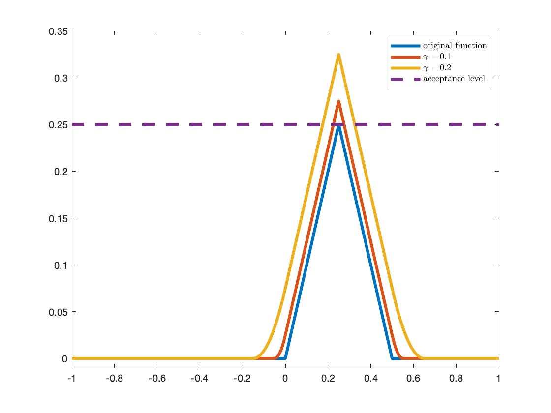
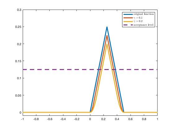
Figure 2: A chance constraint and its approximations (left: restriction; right: relaxation).

While the above examples illustrates that limit points of the sequence of strict local minima of the restricted/relaxed problem may not be a local minimum of the original chance-constrained problem, it is possible to derive a simple result asserting a weak kind of stationarity property of such a limit under minimal assumptions. Phrasing this in a more general context, we consider a parameterized family of closed sets $\{C(w)\}_{w\in{\cal W}}$ and the associated optimization problem:

$${\operatornamewithlimits{\mbox{\bf minimize}}_{x\in C(w)}}\ c_{0}(x),$$ (28)

where the objective function $c_{0}$ is locally Lipschitz continuous. Being fairly straightforward, the next result has two parts: the first part pertains to C-stationary points without assuming convexity; this part is applicable to the families of restricted sets $\{\overline{X}_{\rm rst}(\gamma)\}$ and relaxed sets $\{\overline{X}_{\rm rlx}(\gamma)\}$. The second part pertains to global minimizers when these are computationally meaningful (e.g., when (28) is a convex program); this part is applicable to a family $\{C(\gamma_{\nu};x^{\nu})\}_{\nu=1}^{\infty}$ of surrogate convex feasible sets where $\{x^{\nu}\}$ is a sequence of iterates with each $x^{\nu}$ being associated with the scalar $\gamma_{\nu}>0$.

For each $w\in{\cal W}$, let $\bar{x}^{\rm C}(w)$ be a C-stationary point of (28) and $\bar{x}^{\rm O}(w)$ be a globally optimal solution. Let the sequence $\{w^{\nu}\}$ converge to $w^{\infty}$, and let $\bar{C}(w^{\infty})\triangleq\displaystyle{\limsup_{\nu\to\infty}}\,C(w^{\nu})\triangleq\displaystyle{\bigcap_{\nu\geq 1}}\,\displaystyle{\bigcup_{j\geq\nu}}\,C(w^{j})$. Consider two arbitrary sequences $\{\bar{x}^{\rm C}(w^{\nu})\}$ and $\{\bar{x}^{\rm O}(w^{\nu})\}$ of C-stationary points and global minima, respectively, of the problem (28) corresponding to the sequence $\{w^{\nu}\}$. We are interested in the respective C-stationary and globally minimizing properties of the limit points of these sequences. If the union $\displaystyle{\bigcup_{\nu}}\ C(w^{\nu})$ is bounded, then the two sequences must have convergent subsequences whose limits we take as $\bar{x}^{\rm C}(w^{\infty})$ and $\bar{x}^{\rm O}(w^{\infty})$. It is clear that both limits belong to $\bar{C}(w^{\infty})$.

Proposition 13.

In the above setting, the following two statements hold:

(a) $c_{0}^{\,\circ}\left(\bar{x}^{\rm C}(w^{\infty});v\right)\geq 0$ for all $v\in\displaystyle{\limsup_{\nu\to\infty}}\,{\cal T}\left(\bar{x}^{\rm C}(w^{\nu});C(w^{\nu})\right)$; in particular, if

$${\cal T}\left(\bar{x}^{\rm C}(w^{\infty});\bar{C}(w^{\infty})\right)\,\subseteq\,\displaystyle{\limsup_{\nu\to\infty}}\,{\cal T}\left(\bar{x}^{\rm C}(w^{\nu});C(w^{\nu})\right),$$

then $\bar{x}^{\rm C}(w^{\infty})$ is a C-stationary solution of the limiting problem: $\displaystyle{\operatornamewithlimits{\mbox{\bf minimize}}_{x\in\bar{C}(w^{\infty})}}\ c_{0}(x)$;

(b) $\bar{x}^{\rm O}(w^{\infty})\in\displaystyle{\operatornamewithlimits{\mbox{\bf argmin}}_{x\in\bar{C}(w^{\infty})}}\ c_{0}(x)$.

Proof.

To prove statement (a), let $v\in\displaystyle{\limsup_{\nu\to\infty}}\,{\cal T}\left(\bar{x}^{\rm C}(w^{\nu});C(w^{\nu})\right)$. Then there exist an infinite index set $\kappa$ and a sequence of vectors $\{v^{\nu}\}_{\nu\in\kappa}$ such that $v=\displaystyle{\lim_{\nu(\in\kappa)\to\infty}}\,v^{\nu}$ and $v^{\nu}\in{\cal T}\left(\bar{x}^{\rm C}(w^{\nu});C(w^{\nu})\right)$ for all $\nu\in\kappa$. Therefore, we have

$$c_{0}^{\,\circ}\left(\bar{x}^{\rm C}(w^{\nu});v^{\nu}\right)\,\geq\,0\,\hskip 12.0pt\forall\,\nu\,\in\,\kappa.$$

By (20), we pass to the limit $\nu(\in\kappa)\to\infty$ and obtain the desired C-stationarity property of $\bar{x}^{\rm C}(w^{\infty})$. The second assertion in statement (a) is clear. The proof of statement (b) is similar to that of (a) and omitted. ∎

Example 12 continued. We have ${\cal T}\left(\bar{x}_{\rm rst}(\gamma);\overline{X}_{\rm rst}(\gamma)\right)=\mathbb{R}_{+}$ for all $\gamma\in(0,1/2)$. Since the objective function is the identity function, therefore $c_{0}^{\,\prime}(x;v)=v$ for all pairs $(x,v)\in\mathbb{R}^{2}$; hence the first assertion of Proposition 13(a) is valid, even though the limit of $\bar{x}_{\,\rm rst}(\gamma)$ as $\gamma\downarrow 0$ regrettably has no minimizing property with regards to the original chance-constrained problem (26). Of course, it is possible in this example to obtain the unique global minimizer of the problem if one identifies the global minimizers of the objective function over the various approximating sets $\overline{X}_{\rm rst}(\gamma)$ for $\gamma>0$. From a practical computational perspective, it is in general not possible to identify such a global minimizer when the problem is highly nonconvex and coupled with nondifferentiability. So one has to settle for the computable solutions and understand their properties to the extent possible. $\Box$

A general comment: In the above examples, the feasible regions of the restricted and relaxed problems are each the union of two intervals; due to the simplicity of the objective functions, global minima of the restricted and relaxed problems can therefore be identified and they will converge to the global minima of the respective problems (26) and (27). However, in practical applications, we do not have the luxury of computing the global minima exactly and the best we can settle for are stationary solutions, which under the convexity-like property, are local minima. These examples illustrate that if the restricted/relaxed problems have “bad” local minima, their limits can be very undesirable for the original CCP. In the absence of favorable structures that can be exploited, computing the “sharpest” kind of stationary solutions of the restricted/relaxed/approximated problems, which themselves are most likely nonconvex and nondifferentiable problems too, provides the first step toward obtaining a desirable solution of the given CCP. This important step is the guiding principle for the developments in the rest of the paper.

5 External Sampling: Uniform Exact Penalization

This section develops a uniform exact penalization theory for the following (un-parameterized) expectation constrained stochastic program, without assuming any special structures on the constraint functions except for the well-definedness of the expectation functions and the Lipschitzian properties in Assumption (A_Lip) below. In particular, it covers the relaxed problem (15) and the restricted problem (16) for the CCP with a fixed $\gamma>0$ which we omit in this section. Specifically, we consider

$$\begin{array}[]{ll}\displaystyle{\operatornamewithlimits{\mbox{\bf minimize}}_{x\in X}}&\bar{c}_{0}(x)\,\triangleq\,\mathbb{E}\left[\,c_{0}(x,\tilde{z})\,\right]\\[7.22743pt] \mbox{\bf subject to}&\bar{c}_{k}(x)\,\triangleq\,\underbrace{\mathbb{E}\left[\,c_{k}(x,\tilde{z})\,\right]\,\leq\,\zeta_{k},\hskip 12.0ptk=1,\cdots,K}_{\mbox{constraint set denoted $\widehat{S}$}}.\end{array}$$ (29)

To be self-contained for this section, we restate the blanket assumptions (A_o) and (A_c) in the context of (29):

Assumption (A_Lip) for (29): the functions $\bar{c}_{0}$ and $c_{k}(\bullet,z)$ for all $z\in\Xi$ are directionally differentiable; moreover, the objective function $\bar{c}_{0}$ is Lipschitz continuous on $X$ with constant $\mbox{Lip}_{\rm 0}$ and there exists an integrable function $\mbox{Lip}_{\rm c}\mathrel{\mathop{\ordinarycolon}}\Xi\to\mathbb{R}_{++}$ such that for all $k=1,\cdots,K$,

$$\left|\,c_{k}(x,z)-c_{k}(x^{\prime},z)\,\right|\,\leq\,\mbox{Lip}_{\rm c}(z)\,\left\|\,x-x^{\prime}\,\right\|,\hskip 12.0pt\forall\;x,x^{\prime}\,\in\,X\mbox{ and all }z\,\in\,\Xi.$$

Besides the well-known benefit of transferring the (hard) constraints to the objective, exact penalization is particularly useful in a stochastic setting where the expectation constraints are discretized by sampling. In practice, random sampling of the constraint functions can generate a discretized problem that is not feasible, thus leading to computational difficulties in a solution algorithm. With penalization, this becomes a non-issue. However, penalization raises the question of exactness; that is, can feasibility be recovered with a uniformly finite penalty parameter for all SAA problems with sufficiently large sample sizes? Consistent with our perspective of solving nonconvex problems [14], our analysis below addresses stationary solutions under penalization. We denote the feasible set of (29) by $\widehat{X}\,\triangleq\,X\,\cap\,\widehat{S}$.

Given a penalty parameter $\lambda>0$ applied to the residual function $r_{\rm c}(x)$, we obtain the penalized version of (29):

$${\operatornamewithlimits{\mbox{\bf minimize}}_{x\in X}}\ \bar{c}_{0}(x)+\lambda\,r_{\rm c}(x),\hskip 12.0pt\mbox{where}\hskip 12.0ptr_{\rm c}(x)\,\triangleq\,\displaystyle{\sum_{k=1}^{K}}\,\max\left(\,\bar{c}_{k}(x)-\zeta_{k},\,0\,\right).$$ (30)

Considering the above two problems with the family $\{\bar{c}_{k}(x)\}_{k=0}^{K}$ treated as deterministic functions, we have the following exact penalization result which is drawn from [14, Proposition 9.2.2].

Proposition 14.

Let $X$ be a closed convex set and let $\{\bar{c}_{k}\}_{k=0}^{K}$ be B-differentiable functions defined on an open set containing $X$. Suppose in addition that $\bar{c}_{0}$ is Lipschitz continuous on $X$ with Lipschitz modulus $\mbox{Lip}_{0}>0$. If

$${\operatornamewithlimits{\mbox{\bf supremum}}_{x\,\in\,X\,\setminus\,\widehat{S}}}\ \left[\,\displaystyle{\operatornamewithlimits{\mbox{\bf minimum}}_{v\in{\cal T}(x;X);\,\|v\|=1}}\ r_{\rm c}^{\,\prime}(x;v)\,\right]\,\leq\,-1,$$ (31)

then for every $\lambda>\mbox{Lip}_{0}$, every directional stationary point of (30) is a B-stationary point of (29).

We make several remarks about the condition (31):

(a) It holds that

$$r_{\rm c}^{\,\prime}(x;v)\,=\,\displaystyle{\sum_{k\,\mathrel{\mathop{\ordinarycolon}}\,\bar{c}_{k}(x)\,>\,\zeta_{k}}}\,\bar{c}_{k}^{\,\prime}(x;v)+\displaystyle{\sum_{k\,\mathrel{\mathop{\ordinarycolon}}\,\bar{c}_{k}(x)\,=\,\zeta_{k}}}\,\max\left(\,\bar{c}_{k}^{\,\prime}(x;v),\,0\,\right),\hskip 12.0pt\forall\,(x,v)\,\in\,X\times\mathbb{R}^{n};$$ (32)

(b) $r_{\rm c}^{\,\prime}(x;v)\geq 0$ for all $x\in\widehat{S}$ and all $v\in\mathbb{R}^{n}$ (because the first summation on the right-hand side is vacuous for $x\in\widehat{S}$), this sign property makes it clear that the restriction of $x$ outside the set $\widehat{S}$ is essential in the condition (31).

(c) The condition (31) stipulates that for every $x\in X$ which is infeasible to (29), it is possible to drive $x$ closer to feasibility by reducing the constraint residual function $r_{c}$ starting at $x$ and moving along a descent direction that is tangent to the base set $X$ at $x$. Of course, this condition is intuitively needed for a penalized vector to reach feasibility eventually for finite $\lambda$.

(d) The lower bound $\mbox{Lip}_{0}$ of the penalty parameter $\lambda$ matches the right-hand bound of $-1$ in (31). The essential requirement in obtaining the exactness of the penalization (i.e., a finite lower bound of $\lambda$) is that the left-hand supremum is negative.

5.1 Stochastic penalization for Clarke stationarity

Extending the deterministic treatment, we consider the approximation of the expectation constraint functions by their sample averages, leaving the expected objective function $\bar{c}_{0}$ as is (so that we can focus on the treatment of the constraints). Specifically, given the family of samples $Z^{N}\triangleq\{z^{s}\}_{s=1}^{N}$ of the random variable $\tilde{z}$, we consider

$$\begin{array}[]{ll}\displaystyle{\operatornamewithlimits{\mbox{\bf minimize}}_{x\in X}}&\bar{c}_{0}(x)\\[5.0pt] \mbox{\bf subject to}&c_{k}^{N}(x)\,\triangleq\,\displaystyle{\frac{1}{N}}\,\displaystyle{\sum_{s=1}^{N}}\,c_{k}(x,z^{s})\,\leq\,\zeta_{k},\hskip 12.0ptk\,=\,1,\cdots,K.\end{array}$$ (33)

The penalization of the latter problem with the penalty parameter $\lambda>0$ is:

$${\operatornamewithlimits{\mbox{\bf minimize}}_{x\in X}}\ \bar{c}_{0}(x)+\lambda\,r_{\rm c}^{N}(x),\hskip 12.0pt\mbox{where}\hskip 12.0ptr_{\rm c}^{N}(x)\,\triangleq\,\displaystyle{\sum_{k=1}^{K}}\,\max\left(\,c_{k}^{N}(x)-\zeta_{k},\,0\,\right).$$ (34)

For an arbitrary $x\in X$ and a sample family $Z^{N}$, we define the index sets corresponding to the expectation problem (29) and the SAA problem (33):

$$\begin{array}[]{lll}{\cal A}_{>}(x)\,\triangleq\,\{\,k\in[K]\,\mid\,\bar{c}_{k}(x)\,>\,\zeta_{k}\,\}&\mbox{ versus }&{\cal A}_{>}^{N}(x)\,\triangleq\,\{\,k\in[K]\,\mid\,c_{k}^{N}(x)\,>\,\zeta_{k}\,\}\\[7.22743pt] {\cal A}_{<}(x)\,\triangleq\,\{\,k\in[K]\,\mid\,\bar{c}_{k}(x)\,<\,\zeta_{k}\,\}&\mbox{ versus }&{\cal A}_{<}^{N}(x)\,\triangleq\,\{\,k\in[K]\,\mid\,c_{k}^{N}(x)\,<\,\zeta_{k}\,\}\\[7.22743pt] {\cal A}_{=}(x)\,\triangleq\,\{\,k\in[K]\,\mid\,\bar{c}_{k}(x)\,=\,\zeta_{k}\,\}&\mbox{ versus }&{\cal A}_{=}^{N}(x)\,\triangleq\,\{\,k\in[K]\,\mid\,c_{k}^{N}(x)\,=\,\zeta_{k}\,\}.\end{array}$$

Our goal in what follows is to show that, under appropriate assumptions, for finite values of the penalty parameter $\lambda>0$ (that is independent of $N$), if $\left\{\,\bar{x}^{N,\lambda}\,\right\}_{N=1}^{\infty}$ is a sequence of C-stationary points of (34), then every accumulation point of that sequence is a weak C-stationary point of the expectation constrained problem (29). The latter point is defined as a feasible vector $\bar{x}$ to (29) such that

$$\begin{array}[]{l}\bar{c}_{0}^{\circ}(\bar{x};v)\,\geq\,0,\hskip 12.0pt\forall\;v\,\in\,{\cal T}_{wC}(\bar{x};\widehat{X})\,\triangleq\,\left\{\,v\in\,{\cal T}(\bar{x};X)\,\mid\,\mathbb{E}\left[\,c_{k}(\bullet,\tilde{z})^{\circ}(\bar{x};v)\,\right]\,\leq\,0,\;\forall\;k\in{\cal A}_{=}(\bar{x})\,\right\}.\end{array}$$

We term this as a “weak” C-stationary point because

$$\mathbb{E}\left[\,c_{k}(\bullet,\tilde{z})^{\circ}(x;v)\,\right]\,\geq\,\mathbb{E}\left[\,c_{k}(\bullet,\tilde{z})^{\prime}(x;v)\,\right]\,=\,\left(\,\mathbb{E}\left[\,c_{k}(\bullet,\tilde{z})\,\right]\,\right)^{\prime}(x;v)\,=\,\bar{c}_{k}^{\,\prime}(x;v).$$

Hence, ${\cal T}_{wC}(\bar{x};\widehat{X})\subseteq{\cal L}(\bar{x};\widehat{X})$ with the right-hand (directional derivative based) linearization cone equal to ${\cal T}(\bar{x};\widehat{X})$ under the ACQ for the set $\widehat{X}$ at $\bar{x}$. As we have noted, a sufficient condition for the ACQ to hold is that the directional Slater CQ holds; i.e., if

$$\mbox{cl}\left\{\,v\,\in\,{\cal T}(\bar{x};X)\,\mid\,\bar{c}_{k}^{\,\prime}(\bar{x};v)<0,\,\,\forall\ k\in{\cal A}_{=}(\bar{x})\,\right\}\,=\,{\cal L}(\bar{x};\widehat{X}).$$

It therefore follows that if these CQs hold for the set $\widehat{X}$ at $\bar{x}$, and if $\bar{x}$ is a C-stationary point as defined in Subsection 4.1, then $\bar{x}$ must be a weak C-stationary point; the converse holds if $c_{k}(\bullet,z)$ is Clarke regular for almost every $z\in\Xi$ so that the two cones ${\cal T}_{wC}(\bar{x};\widehat{X})$ and ${\cal L}(\bar{x};\widehat{X})$ are equal. This connection with C-stationarity explains the adjective “weak”.

In terms of the above defined index sets, we have

$$\begin{array}[]{ll}(\,r_{\rm c}^{N}\,)^{\,\prime}(x;v)&=\,\displaystyle{\sum_{k\,\in\,{\cal A}_{>}^{N}(x)}}\,(c_{k}^{N})^{\prime}(x;v)+\displaystyle{\sum_{k\,\in\,{\cal A}_{=}^{N}(x)}}\,\max\left(\,(c_{k}^{N})^{\prime}(x;v),\,0\,\right)\\[14.45377pt] &=\displaystyle{\sum_{k\,\in\,{\cal A}_{>}^{N}(x)}}\,{\displaystyle{\frac{1}{N}}\,\displaystyle{\sum_{s=1}^{N}}\,c_{k}(\bullet,z^{s})^{\prime}(x;v)}+\displaystyle{\sum_{k\,\in\,{\cal A}_{=}^{N}(x)}}\,\max\left(\,\displaystyle{\frac{1}{N}}\,\displaystyle{\sum_{s=1}^{N}}\,c_{k}(\bullet,z^{s})^{\prime}(x;v),\,0\,\right).\end{array}$$

Note that unlike ${\cal A}_{>}(x)$ and ${\cal A}_{=}(x)$ which are deterministic index sets in (32) for the directional derivative of the expectation function, ${\cal A}_{>}^{N}(x)$ and ${\cal A}_{=}^{N}(x)$ are sample-dependent index sets. Using the Clarke directional derivative, we define, for any $x\in X$ and $v$ in $\mathbb{R}^{n}$,

$$\begin{array}[]{rll}(\,\widehat{r}_{\rm c}^{\,N}\,)^{\circ}(x;v)&\triangleq\displaystyle{\sum_{k\,\in\,{\cal A}_{>}^{N}(x)}}\,\displaystyle{\frac{1}{N}}\,\displaystyle{\sum_{s=1}^{N}}\,c_{k}(\bullet,z^{s})^{\circ}(x;v)+\displaystyle{\sum_{k\,\in\,{\cal A}_{=}^{N}(x)}}\,\max\left(\,\displaystyle{\frac{1}{N}}\,\displaystyle{\sum_{s=1}^{N}}\,c_{k}(\bullet,z^{s})^{\circ}(x;v),\,0\,\right)\\[18.06749pt] \widehat{r}_{\rm c}^{\,\circ}(x;v)&\triangleq\displaystyle{\sum_{k\,\in\,{\cal A}_{>}(x)}}\,\mathbb{E}\left[\,c_{k}(\bullet,\tilde{z})^{\circ}(x;v)\,\right]+\displaystyle{\sum_{k\,\in\,{\cal A}_{=}(x)}}\,\max\left(\,\mathbb{E}\left[\,c_{k}(\bullet,\tilde{z})^{\circ}(x;v)\,\right],\,0\,\right).\end{array}$$ (35)

Notice that in general $(\,\widehat{r}_{\rm c}^{N}\,)^{\circ}(x;v)$ is not equal to $(\,r_{\rm c}^{N}\,)^{\circ}(x;v)$ due to the failure of the additivity of the Clarke directional derivative in terms of the directions; nevertheless, we have

$$(\,\widehat{r}_{\rm c}^{N}\,)^{\circ}(x;v)\,\geq\,(\,r_{\rm c}^{N}\,)^{\circ}(x;v)\,\geq\,(r_{\rm c}^{N})^{\prime}(x;v),\hskip 12.0pt\forall\,(x,v)\,\in\ X\,\times\,\mathbb{R}^{n};$$ (36)

similar inequalities hold for the residual of the expectation constraint functions.

Given two sets $A$ and $B$ in $\mathbb{R}^{n}$, we denote the (one-side) deviation of $A$ from $B$ as

$$\mathbb{D}(A,B)\,\triangleq\,\sup_{x\in A}\,\mbox{dist}(x,B)\,=\,\sup_{x\in A}\,\inf_{y\in B}\,\|\,x-y\,\|.$$

The following lemma is a direct consequence of [58, Theorem 2]. In the lemma, we write $\partial_{C}c_{k}(x,z)$ for the Clarke subdifferential of $c_{k}(\bullet,z)$ at $x$.

Lemma 15.

Let $X$ be a compact set and let (A_Lip) hold. Let $\{z^{s}\}_{s=1}^{\infty}$ be independent realizations of the random vector $\tilde{z}$. For any $v\in\mathbb{R}^{n}$, it holds that for all $k=1,\cdots,K$,

$${\limsup_{N\to\infty}}\,\displaystyle{\sup_{x\in X}}\,\left(\,\displaystyle{\frac{1}{N}}\,\displaystyle{\sum_{s=1}^{N}}\,c_{k}(\bullet,z^{s})^{\circ}(x;v)-\mathbb{E}\left[\,c_{k}(\bullet,\tilde{z})^{\circ}(x;v)\,\right]\,\right)\,\leq\,0\hskip 12.0pt\mbox{almost surely}.$$

Proof.

It follows from [58, Theorem 2] that for any $\delta>0$,

$$\sup_{x\in X}\,\mathbb{D}\left(\,\displaystyle{\frac{1}{N}}\,\displaystyle{\sum_{s=1}^{N}}\,\partial_{C}\,c_{k}(x,z^{s}),\,\displaystyle{\bigcup_{x^{\prime}\in\mathbb{B}_{\delta}(x)}}\,\mathbb{E}\left[\,\partial_{C}\,c_{k}(x^{\prime},\tilde{z})\,\right]\,\right)\to 0\hskip 12.0pt\mbox{as $N\to\infty$}\hskip 12.0pt\mbox{almost surely}.$$

Consider any $v\in\mathbb{R}^{n}$ and any $\delta>0$. Since for any $x\in X$ and any $z\in\Xi$,

$$\partial_{C}\,c_{k}(x,z)\,=\,\left\{\,a\,\in\,\mathbb{R}^{n}\,\mid\,c_{k}(\bullet,z)^{\circ}(x;v)\,\geq\,a^{\top}v,\;\ \forall\;v\,\in\,\mathbb{R}^{n}\,\right\},$$

we derive that for any $x\in X$, $v\in\mathbb{R}^{n}$, and $\varepsilon>0$, there exist a positive integer $\overline{N}$ independent of $x$, vectors $\{a^{s}\in\partial_{C}\,c_{k}(x,z^{s})\}_{s=1}^{N}$ and $\bar{a}\in\displaystyle{\bigcup_{x^{\prime}\in\mathbb{B}_{\delta}(x)}}\,\mathbb{E}\left[\,\partial_{C}\,c_{k}(x^{\prime},\tilde{z})\,\right]$ such that for all $N\geq\overline{N}$,

$$\begin{array}[]{rl}\displaystyle{\frac{1}{N}}\,\displaystyle{\sum_{s=1}^{N}}\,c_{k}(\bullet,z^{s})^{\circ}(x;v)\,=&\displaystyle{\frac{1}{N}}\,\displaystyle{\sum_{s=1}^{N}}\,(a^{s})^{\top}v\,\leq\,\bar{a}^{\top}v+\varepsilon\,\leq\,\displaystyle{\limsup_{x^{\prime}\in\mathbb{B}_{\delta}(x)}}\,\mathbb{E}\left[\,c_{k}(\bullet,\tilde{z})^{\circ}(x^{\prime};v)\,\right]+\varepsilon.\end{array}$$

We can thus derive the stated result by taking $N\to\infty$, $\varepsilon\downarrow 0$, and using the upper semicontinuity of the Clarke directional derivative. ∎

The above lemma yields the following sequential generalization of the pointwise inequalities (36).

Lemma 16.

Let $X$ be a compact set and let (A_Lip) hold. Then for any $v\in\mathbb{R}^{n}$ and every sequence $\{x^{N}\}\subseteq X$ converging to $\bar{x}\in X$, it holds that

$${\limsup_{N\to\infty}}\,(\,\widehat{r}_{\rm c}^{\,N}\,)^{\circ}(x^{N};v)\,\leq\,\widehat{r}_{c}^{\,\circ}(\bar{x};v)\hskip 12.0pt\mbox{almost surely}.$$

Proof.

It follows from the uniform law of large numbers (cf. [57, Theorem 7.48]) that

$$\begin{array}[]{l}\displaystyle{\lim_{N\to\infty}}\,\displaystyle{\sup_{x\in X}}\,\left|\,c_{k}^{N}(x)-\bar{c}_{k}(x)\,\right|\,=\,0\hskip 12.0pt\mbox{almost surely},\hskip 12.0pt\forall\,k\,=\,1,\cdots,K.\end{array}$$ (37)

Since we have

$$c_{k}^{N}(x^{N})-\bar{c}_{k}(\bar{x})\,=\,\left[\,c_{k}^{N}(x^{N})-\bar{c}_{k}(x^{N})\,\right]+\left[\,\bar{c}_{k}(x^{N})-\bar{c}_{k}(\bar{x})\,\right],$$

we may obtain, by the continuity of $c_{k}(\bullet,z^{s})$, that for all $N$ sufficiently large,

$${\cal A}_{>}(\bar{x})\,\subseteq\,{\cal A}_{>}^{N}(x^{N})\hskip 12.0pt\mbox{and}\hskip 12.0pt{\cal A}_{>}^{N}(x^{N})\,\cup\,{\cal A}_{=}^{N}(x^{N})\,\subseteq\,{\cal A}_{>}(\bar{x})\,\cup\,{\cal A}_{=}(\bar{x})\hskip 12.0pt\mbox{almost surely}.$$

The first inclusion rules out that an index $k\in{\cal A}_{=}^{N}(x^{N})$ belongs to ${\cal A}_{>}(\bar{x})$. Hence, for any $\varepsilon>0$, there exists a sufficiently large $N$ such that the following string of inequalities hold almost surely:

$$\begin{array}[]{rl}(\,\widehat{r}_{\rm c}^{\,N}\,)^{\circ}(x^{N};v)\,=&\displaystyle{\sum_{k\,\in\,{\cal A}_{{\color[rgb]{0,0,0}>}}^{N}(x^{N})}}\displaystyle{\frac{1}{N}}\,\displaystyle{\sum_{s=1}^{N}}\,c_{k}(\bullet,z^{s})^{\circ}(x^{N};v)+\displaystyle{\sum_{k\,\in\,{\cal A}_{=}^{N}(x^{N})}}\,\max\left(\,\displaystyle{\frac{1}{N}}\,\displaystyle{\sum_{s=1}^{N}}\,c_{k}(\bullet,z^{s})^{\circ}(x^{N};v),\,0\,\right)\\[21.68121pt] \leq&\displaystyle{\sum_{k\,\in\,{\cal A}_{{\color[rgb]{0,0,0}>}}(\bar{x})}}\displaystyle{\frac{1}{N}}\,\displaystyle{\sum_{s=1}^{N}}\,c_{k}(\bullet,z^{s})^{\circ}(x^{N};v)+\displaystyle{\sum_{k\,\in\,{\cal A}_{=}(\bar{x})}}\,\max\left(\,\displaystyle{\frac{1}{N}}\,\displaystyle{\sum_{s=1}^{N}}\,c_{k}(\bullet,z^{s})^{\circ}(x^{N};v),\,0\,\right)\\[21.68121pt] \leq&\displaystyle{\sum_{k\,\in\,{\cal A}_{{\color[rgb]{0,0,0}>}}(\bar{x})}}\,\mathbb{E}\,\left[\,c_{k}(\bullet,\tilde{z})^{\circ}(x^{N};v)\,\right]+\displaystyle{\sum_{k\,\in\,{\cal A}_{=}(\bar{x})}}\,\max\left(\,\mathbb{E}\,\left[\,c_{k}(\bullet,\tilde{z})^{\circ}(x^{N};v)\,\right],\,0\,\right)\ +\\[21.68121pt] &\hskip 12.0pt\displaystyle{\sum_{k=1}^{K}}\,\max\left(\,\displaystyle{\frac{1}{N}}\,\displaystyle{\sum_{s=1}^{N}}\,c_{k}(\bullet,z^{s})^{\circ}(x^{N};v)-\mathbb{E}\left[\,c_{k}(\bullet,\tilde{z})^{\,\circ}(x^{N};v)\,\right],\,0\,\right)\\[21.68121pt] \leq&\displaystyle{\sum_{k\,\in\,{\cal A}_{{\color[rgb]{0,0,0}>}}(\bar{x})}}\,\mathbb{E}\,\left[\,c_{k}(\bullet,\tilde{z})^{\circ}(x^{N};v)\,\right]+\displaystyle{\sum_{k\,\in\,{\cal A}_{=}(\bar{x})}}\,\max\left(\,\mathbb{E}\,\left[\,c_{k}(\bullet,\tilde{z})^{\circ}(x^{N};v)\,\right],\,0\,\right)+\varepsilon,\end{array}$$

where the last inequality is due to Lemma 15. By the upper semicontinuity (20) of the Clarke directional derivative, the desired conclusion follows. ∎

For each pair $(Z^{N},\lambda)$, let $\bar{x}^{N,\lambda}$ be a C-stationary point of (34). The result below shows that a finite $\bar{\lambda}>0$ exists such that for all $\lambda>\bar{\lambda}$, every accumulation point of the sequence $\{\bar{x}^{N,\lambda}\}$ is feasible for (29) and is a weak C-stationary point of this expectation-constrained problem. The proof of this result is based on the above two technical lemmas and by strengthening the sufficient condition (31). Note that the result does not address how the iterate $\bar{x}^{N,\lambda}$ is obtained. Thus, the result is in the spirit of the convergence analysis of an SAA scheme, albeit it pertains to a stationary point as opposed to a minimizer.

Proposition 17.

Let $X$ be a polyhedron. Assume that (A_Lip) holds and

$${\operatornamewithlimits{\mbox{\bf supremum}}_{x\,\in\,X\,\setminus\,\widehat{S}}}\ \left[\,\displaystyle{\operatornamewithlimits{\mbox{\bf minimum}}_{v\in{\cal T}(x;X);\,\|v\|=1}}\ \widehat{r}_{\rm c}^{\,\circ}(x;v)\,\right]\,\leq\,-1,$$ (38)

where $\widehat{r}_{c}^{\,\circ}(x;v)$ is defined in (35). Then, for every $\lambda>\mbox{Lip}_{0}$, the following three statements hold for any accumulation point $\bar{x}^{\lambda}$ of the sequence $\{\bar{x}^{N,\lambda}\}_{N=1}^{\infty}$:

(a) $\bar{x}^{\lambda}\in\widehat{S}$ almost surely; thus $\bar{x}^{\lambda}$ is feasible to (29) almost surely;

(b) $\bar{x}^{\lambda}$ is a weak C-stationary point of (29) almost surely;

(c) if for almost every $z\in\Xi$, each function in the family $\{c_{k}(\bullet,z)\}_{k=0}^{K}$ is Clarke regular at $\bar{x}^{\lambda}$, then $\bar{x}^{\lambda}$ is a B-stationary point of (29) almost surely.

Proof.

The C-stationarity condition at $\bar{x}^{N,\lambda}$ of (34) implies that

$$(\,\bar{c}_{0}\,)^{\circ}(\bar{x}^{N,\lambda};v)+\lambda\,(r^{N}_{\rm c})^{\circ}(\bar{x}^{N,\lambda};v)\,\geq\,0,\hskip 12.0pt\forall\,v\,\in\,{\cal T}(\bar{x}^{N,\lambda};X).$$ (39)

For simplicity, we assume that $\bar{x}^{\lambda}$ is the limit of the sequence $\{\bar{x}^{N,\lambda}\}$. We claim that $\bar{x}^{\lambda}\in\widehat{S}$ almost surely. Assume by contradiction that there exists positive probability such that $\bar{x}^{\lambda}\not\in\widehat{S}$. Then restricted to the event where $\bar{x}^{\lambda}\not\in\widehat{S}$, there exists $\bar{v}\in{\cal T}(\bar{x}^{\lambda};X)$ with $\|\bar{v}\|=1$ such that

$$\widehat{r}_{\rm c}^{\,\circ}(\bar{x}^{\lambda};\bar{v})\,\leq\,-1.$$

Since $X$ is a polyhedron, it follows that with $N$ sufficiently large, $\bar{v}$ belongs to ${\cal T}(x^{N,\lambda};X)$. Let $\varepsilon\in\left(\,0,\,1-\displaystyle{\frac{\mbox{Lip}_{0}}{\lambda}}\,\right)$. Then from Lemma 16, there exists $N$ such that $(r_{c}^{N})^{\circ}(\bar{x}^{N,\lambda};\bar{v})\leq\widehat{r}_{c}^{\,\circ}(\bar{x}^{\lambda};\bar{v})+\varepsilon$ almost surely. By substituting $v=\bar{v}$ into (39) and noting $|\,(\,\bar{c}_{0}\,)^{\circ}(\bar{x}^{N,\lambda};\bar{v})\,|\,\leq\,\mbox{Lip}_{0}\,\|\,\bar{v}\,\|\,=\,\mbox{Lip}_{0}$, we deduce

$$0\leq\mbox{Lip}_{0}+\lambda\,\left(\,\widehat{r}_{\rm c}^{\,\circ}(\bar{x}^{\lambda};\bar{v})+\varepsilon\,\right)\,\leq\,\mbox{Lip}_{0}+\lambda\,\left(\,-1+\varepsilon\,\right)\,<\,0,$$

which is a contradiction. Therefore, $\bar{x}^{\lambda}\in\widehat{S}$ almost surely. To show the claimed weak C-stationarity of $\bar{x}^{\lambda}$ for the problem (29), let $v\in{\cal T}_{wC}(\bar{x}^{\lambda};X\,\cap\,\widehat{S})$ be arbitrary with unit length. For such a tangent vector $v$, we have $\mathbb{E}\,\left[\,c_{k}(\bullet,\tilde{z})^{\,\circ}(\bar{x}^{\lambda};v)\,\right]\leq 0$ for all $k\in{\cal A}_{=}(\bar{x}^{\lambda})$. Moreover, since $\bar{x}^{\lambda}\in\widehat{S}$, thus ${\cal A}_{>}(\bar{x}^{\lambda})=\emptyset$, we have ${\cal A}_{>}^{N}(\bar{x}^{N,\lambda})\,\cup\,{\cal A}_{=}^{N}(\bar{x}^{N,\lambda})\,\subseteq{\cal A}_{=}(\bar{x}^{\lambda})$ for all $N$ sufficiently large almost surely. Hence, for any $\varepsilon^{\,\prime}>0$ and sufficiently large $N$, the following inequalities hold almost surely:

$$\begin{array}[]{rl}0\,\leq&\Bigg{(}\,\bar{c}_{0}(\bullet)+\lambda\,\displaystyle{\sum_{k\in{\cal A}_{>}^{N}(\bar{x}^{N,\lambda})}}\,c_{k}^{N}(\bullet\,;v)+\lambda\,\displaystyle{\sum_{k\in{\cal A}_{=}^{N}(\bar{x}^{N,\lambda})}}\,\max\left(\,c_{k}^{N}(\bullet\,;v),0\,\right)\,\Bigg{)}^{\circ}(\bar{x}^{N,\lambda};v)\\[21.68121pt] \leq&(\,\bar{c}_{0}\,)^{\circ}(\bar{x}^{N,\lambda};v)+\lambda\,\displaystyle{\sum_{k\,\in\,{\cal A}_{=}(\bar{x}^{\lambda})}}\,\max\left(\,(\,c_{k}^{N}\,)^{\circ}(\bar{x}^{N,\lambda};v),\,0\,\right)\\[18.06749pt] \leq&(\,\bar{c}_{0}\,)^{\circ}(\bar{x}^{N,\lambda};v)+\lambda\,\displaystyle{\sum_{k\,\in\,{\cal A}_{=}(\bar{x}^{\lambda})}}\,\max\Bigg{(}\,\displaystyle{\frac{1}{N}}\,\displaystyle{\sum_{s=1}^{N}}\,c_{k}(\bullet,z^{s})^{\circ}(\bar{x}^{N,\lambda};v)-\mathbb{E}\left[\,c_{k}(\bullet,\tilde{z})^{\circ}(\bar{x}^{N,\lambda};v)\,\right],\,0\,\Bigg{)}\\[21.68121pt] &+\,\lambda\,\displaystyle{\sum_{k\,\in\,{\cal A}_{=}(\bar{x}^{\lambda})}}\,\max\left(\,\mathbb{E}\left[\,c_{k}(\bullet,\tilde{z})^{\circ}(\bar{x}^{N,\lambda};v)\,\right]-\mathbb{E}\left[\,c_{k}(\bullet,\tilde{z})^{\circ}(\bar{x}^{\lambda};v)\,\right],\,0\,\right)\\[18.06749pt] \leq&(\,\bar{c}_{0}\,)^{\circ}(\bar{x}^{N,\lambda};v)+\lambda\,\varepsilon^{\,\prime}+\lambda\,\displaystyle{\sum_{k\,\in\,{\cal A}_{=}(\bar{x}^{\lambda})}}\,\max\left(\,\mathbb{E}\,\left[\,c_{k}(\bullet,\tilde{z})^{\circ}(\bar{x}^{N,\lambda};v)-c_{k}(\bullet,\tilde{z})^{\circ}(\bar{x}^{\lambda};v)\,\right],\,0\,\right).\end{array}$$

Letting $N\to\infty$ and using the upper semicontinuity of the Clarke directional derivative at $\bar{x}^{\lambda}$, we deduce that almost surely,

$$(\,\bar{c}_{0}\,)^{\circ}(\bar{x}^{\lambda};v)\,\geq\,0,\hskip 12.0pt\forall\,v\,\in\,{\cal T}_{wC}(\bar{x}^{\lambda};X\,\cap\,\widehat{S}),$$

which is the almost sure weak C-stationarity of $\bar{x}^{\lambda}$ for the problem (29).

To prove part (c), as we have already noted that, under the Clarke regularity of $\{c_{k}(\bullet,z)\}_{k=1}^{K}$ at $\bar{x}^{\lambda}$ for almost all $z\in\Xi$, we have ${\cal T}_{wC}(\bar{x}^{\lambda};X\,\cap\,\widehat{S})={\cal L}(\bar{x}^{\lambda};X\,\cap\,\widehat{S})$. Hence, by (b), it follows that $(\,\bar{c}_{0}\,)^{\circ}(\bar{x}^{\lambda};v)\geq 0$ for all $v\in{\cal L}(\bar{x}^{\lambda};X\,\cap\,\widehat{S})\supseteq{\cal T}(\bar{x}^{\lambda};X\,\cap\,\widehat{S})$. Since

$$\begin{array}[]{lll}\left(\,\mathbb{E}\,\left[\,c_{0}(\bullet,\tilde{z})\,\right]\,\right)^{\prime}(\bar{x}^{\lambda};v)&=&\mathbb{E}\,\left[\,c_{0}(\bullet,\tilde{z})^{\prime}(\bar{x}^{\lambda};v)\,\right]\\[7.22743pt] &=&\mathbb{E}\,\left[\,c_{0}(\bullet,\tilde{z})^{\circ}(\bar{x}^{\lambda};v)\,\right]\hskip 12.0pt\mbox{by Clarke regularity of $c_{0}(\bullet,z)$ at $\bar{x}^{\lambda}$}\\[7.22743pt] &=&\left(\,\mathbb{E}\,\left[\,c_{0}(\bullet,\tilde{z})\,\right]\,\right)^{\circ}(\bar{x}^{\lambda};v)\hskip 12.0pt\mbox{by \cite[cite]{[\@@bibref{}{ShapiroDentchevaRuszczynski09}{}{}, Theorem~{}7.68]}},\end{array}$$

the claimed B-stationary of $\bar{x}^{\lambda}$ for (29) almost surely follows readily. ∎

6 Sequential Sampling with Majorization

In this section, we are interested in the combination of sequential sampling, penalization (with variable penalty parameter) and upper surrogation to solve the CCP in (1) via the restricted (16) and relaxed (15) problems. We propose an algorithm based on the unified formulation (14) of the latter problems; we also recall the blanket assumptions for (14). Closely related to majorization minimization that is the basis of popular “linearization” algorithms for solving dc programs, [31, 32, 45], the basic idea of surrogation for solving a nonconvex nondifferentiable optimization problem is to derive upper bounding functions of the functions involved, followed by the solution of a sequence of subproblems by convex programming methods. When this solution strategy is applied to the problem (14), there are two most important points to keep in mind:

(a) Although in the context of the relaxed $c_{k\ell}^{\rm rlx}(\bullet,z;\gamma)$ and restricted $c_{k\ell}^{\rm rst}(\bullet,z;\gamma)$ functions, their unifications $c_{k\ell}(\bullet,z;\gamma)$ are dc in theory, their practical dc decompositions are not easily available for the purpose of computations (unless the indicator function is relaxed/restricted by piecewise affine functions; see Lemma 1.)

(b) The resulting expectation functions $\bar{c}_{k}(\bullet;\gamma)$ appear in the constraints; the standard dc approach as described in the cited references would lump all such constraints into the objective via infinity-valued indicator functions. Even if the explicit dc representations of the constraint functions are available, the resulting dc algorithm is at best a conceptual procedure not readily implementable in practice.

To address the former point—lack of explicit dc representation, the extended idea of “surrogation” is used of which the dc-like linearization is a special case. A comprehensive treatment of the “surrogation approach” for solving nonconvex nondifferentiable optimization problems is detailed in [14, Chapter 7]. To address the second point—proper treatment of the chance constraints, we employ exact penalization (i.e., finite value of the penalty parameter) with the aim of recovering solutions of the original CCP (14); furthermore, due to the nonconvexity of the functions involved, recovery is with reference to stationary solutions instead of minimizers, as exemplified by the results in Section 5. When these considerations are combined with the need of sampling to handle the expectation operator, the end result is the Sampling + Penalization + Surrogation Algorithm (SPSA) to be introduced momentarily. We remark that while the cited monograph and the reference [43] have discussed a solution approach for a deterministic dc program based on the linearization of the constraints without penalization, in the context where sampling is needed, this direct treatment of constraints runs the risk of infeasible sampled subproblems that is avoided by the penalization approach.

For any given pair $(\bar{x},z)\in X\times\Xi$ and $k\in[K]$, we let $\widehat{c}_{k}(\bullet,z;\gamma;\bar{x})$ be a majorization of the function $c_{k}(\bullet,z;\gamma)$ at $\bar{x}$ satisfying

(a) [B-differentiability] $\widehat{c}_{k}(\bullet,z;\gamma;\bar{x})$ is B-differentiable on $X$;

(b) [upper surrogation] $\widehat{c}_{k}(x,z;\gamma;\bar{x})\geq c_{k}(x,z;\gamma)$ for all $x\in X$;

(c) [touching condition] $\widehat{c}_{k}(\bar{x},z;\gamma;\bar{x})=c_{k}(\bar{x},z;\gamma)$;

(d) [upper semicontinuity] $\widehat{c}_{k}(\bullet,z;\gamma;\bullet)$ is upper semicontinuous on $X\times X$; and

(e) [directional derivative consistency] $\widehat{c}_{k}^{\,\prime}(\bullet,z;\gamma;\bar{x})(\bar{x};d)=c_{k}^{\,\prime}(\bullet,z;\gamma)(\bar{x};d)$ for any $d\in\mathbb{R}^{n}$.

Starting with the respective summands $c_{k\ell}^{\rm rlx}(x,z;\gamma)$ and $c_{k\ell}^{\rm rst}(x,z;\gamma)$ given in (10), there are several ways to construct majorization functions for the relaxed $c_{k}^{\rm rlx}(x,z;\gamma)\triangleq\displaystyle{\sum_{\ell=1}^{L}}\,c_{k\ell}^{\rm rlx}(x,z;\gamma)$ and restricted $c_{k}^{\rm rst}(x,z;\gamma)\triangleq\displaystyle{\sum_{\ell=1}^{L}}\,c_{k\ell}^{\rm rst}(x,z;\gamma)$ functions that satisfy the conditions. Details can be found in Appendix 1; see also Subsection 6.2.3. In what follows, we assume that the surrogation functions $\widehat{c}_{k}(x,z;\gamma;\bar{x})$ are given. We also assume a similar surrogation function $\widehat{c}_{0}(\bullet,z;\bar{x})$ of $c_{0}(\bullet,z)$ in the objective satisfying the same five conditions. Denote

$$\begin{array}[]{lll}V_{\lambda}(x,Z^{N};\gamma)&\triangleq&\displaystyle{\frac{1}{N}}\,\displaystyle{\sum_{s=1}^{N}}\,c_{0}(x,z^{s})+\lambda\,{\color[rgb]{0,0,0}\displaystyle{\sum_{k=1}^{K}}}\,\max\left\{\,\displaystyle{\frac{1}{N}}\,\displaystyle{\sum_{s=1}^{N}}\,c_{k}(x,z^{s};\gamma)-\zeta_{k},\,0\,\right\}\\[21.68121pt] \widehat{V}_{\lambda}(x,Z^{N};\gamma;\bar{x})&\triangleq&\displaystyle{\frac{1}{N}}\,\displaystyle{\sum_{s=1}^{N}}\,\widehat{c}_{0}(x,z^{s};\bar{x})+\lambda\,{\color[rgb]{0,0,0}\displaystyle{\sum_{k=1}^{K}}}\,\max\left(\,\displaystyle{\frac{1}{N}}\,\displaystyle{\sum_{s=1}^{N}}\,\widehat{c}_{k}(x,z^{s};\gamma;\bar{x})-\zeta_{k},\,0\,\right)\\[21.68121pt] \widehat{V}_{\lambda}^{\rho}(x,Z^{N};\gamma;\bar{x})&\triangleq&\widehat{V}_{\lambda}(x,Z^{N};\gamma;\bar{x})+\displaystyle{\frac{\rho}{2}}\,\|\,x-\bar{x}\,\|^{2},\hskip 12.0pt\mbox{for $\rho>0$}.\end{array}$$ (40)

Notice that in the context of the relaxed/restricted functions $c_{k\ell}^{\rm rlx/rst}(x,z;\gamma)$, the surrogate functions $\widehat{c}_{k}(x,z^{s};\gamma;\bar{x})$ given in Appendix 1 are the pointwise minimum of finitely many convex functions. Thus, a global minimizer of the problem

$${\operatornamewithlimits{\mbox{\bf minimize}}_{x\in X}}\ \widehat{V}_{\lambda}^{\rho}(x,Z^{N};\gamma;\bar{x})$$ (41)

can be obtained by solving finitely many convex programs (see Appendix 2 for an explanation how this is carried out). This is an important practical aspect of the SPSA; namely, the iterates can be constructively obtained by convex programming algorithms.

In the algorithm below, we present the version where the subproblems (41) are solved to global optimality without requiring the uniqueness of the minimizer. The algorithm makes use of several sequences: $\{N_{\nu}\}_{\nu=1}^{\infty}$ (sample sizes), $\{\lambda_{\nu}\}_{\nu=1}^{\infty}$ (penalty parameters), $\{\rho_{\nu}\}_{\nu=1}^{\infty}$ (proximal parameters), and $\{\gamma_{\nu}\}_{\nu=1}^{\infty}$ (scaling factors), as specified below:

$\bullet$ $\{N_{\nu}\}_{\nu=0}^{\infty}$: an increasing sequence of positive integers with $N_{0}=0$; each $N_{\nu}$ denotes the sample batch size at the $\nu$th iteration;

$\bullet$ $\{\lambda_{\nu}\}_{\nu=1}^{\infty}$: a nondecreasing sequence of positive scalars with $\lambda_{1}=1$ and $\displaystyle{\lim_{\nu\to\infty}}\,\lambda_{\nu}=\lambda_{\infty}\in[\,1,\infty\,]$ (this includes both a bounded and unbounded sequence);

$\bullet$ $\{\rho_{\nu}\}_{\nu=1}^{\infty}$: a sequence of positive scalars with $\displaystyle{\lim_{\nu\to\infty}}\,\rho_{\nu}=\rho_{\infty}\in[\,0,\infty\,)$ and such that for some constants $\alpha_{2}>\alpha_{1}>0$,

$${\frac{\alpha_{1}}{\nu}}\,\leq\,\displaystyle{\frac{\rho_{\nu}}{\lambda_{\nu}}}\,\leq\,\displaystyle{\frac{\alpha_{2}}{\nu}},\hskip 12.0pt\forall\,\nu;$$ (42)

$\bullet$ $\{\gamma_{\nu}\}_{\nu=1}^{\infty}$: a nonincreasing sequence of positive values with $\displaystyle{\lim_{\nu\to\infty}}\,\gamma_{\nu}=\underline{\gamma}\geq 0$; moreover, the sum

$${\sum_{\nu=1}^{\infty}}\,\displaystyle{\sup_{x\in X}}\,\Bigg{|}\,\underbrace{\mathbb{E}\left[\,c_{k}(x,\tilde{z};\gamma_{\nu})-c_{k}(x,\tilde{z};\gamma_{\nu-1})\,\right]}_{\mbox{ $=\bar{c}_{k}(x,\gamma_{\nu})-\bar{c}_{k}(x,\gamma_{\nu-1})$}}\Bigg{|}$$ (43)

is finite.

Note that the condition (42) implies:

$${\lim_{\nu\to\infty}}\,\displaystyle{\frac{\rho_{\nu}}{\lambda_{\nu}}}\,=\,0\hskip 12.0pt\mbox{and}\hskip 12.0pt\displaystyle{\sum_{\nu=1}^{\infty}}\,\displaystyle{\frac{\rho_{\nu}}{\lambda_{\nu}}}\,\,=\,\infty.$$ (44)

In particular, such condition permits $\{\lambda_{\nu}\}$ to stay bounded while $\{\rho_{\nu}\}\downarrow 0$, and also the opposite situation where $\{\rho_{\nu}\}$ is bounded away from zero while $\{\lambda_{\nu}\}\to\infty$. Condition (43) holds trivially if $\gamma_{\nu}=\gamma_{\nu-1}$ for all $\nu$ sufficiently large, in particular, when the sequence $\{\gamma_{\nu}\}$ is a constant. In the context of the restricted/relaxed approximations of the probability constraints, we recall Proposition 6 that yields, with $\gamma_{\nu-1}\geq\gamma_{\nu}$,

$$\begin{array}[]{lll}\left|\,\bar{c}_{k}^{\,\rm rst/rlx}(x;\gamma_{\nu})-\bar{c}_{k}^{\,\rm rst/rlx}(x;\gamma_{\nu-1})\,\right|\\[7.22743pt] \leq\,{\mbox{Lip}_{\theta}}\,\displaystyle{\sum_{\ell=1}^{L}}\ |\,e_{k\ell}\,|\,\max\left(\,h_{{\cal Z}_{\ell}(x,\bullet)}^{\rm ub}(\gamma_{\nu})-h_{{\cal Z}_{\ell}(x,\bullet)}^{\rm ub}(\gamma_{\nu-1}),\ h_{{\cal Z}_{\ell}(x,\bullet)}^{\rm lb}(\gamma_{\nu-1})-h_{{\cal Z}_{\ell}(x,\bullet)}^{\rm lb}(\gamma_{\nu})\,\right),\end{array}$$

see (8) for the definitions of the functions $h_{Z}^{\rm lb/ub}(\gamma)$ associated with the random variable $Z\triangleq{\cal Z}_{\ell}(x,\bullet)$. Hence, condition (43) holds if for all $\ell\in[L]$,

$${\sum_{\nu=1}^{\infty}}\,\displaystyle{\sup_{x\in X}}\,\max\left(\,h_{{\cal Z}_{\ell}(x,\bullet)}^{\rm ub}(\gamma_{\nu})-h_{{\cal Z}_{\ell}(x,\bullet)}^{\rm ub}(\gamma_{\nu-1}),\ h_{{\cal Z}_{\ell}(x,\bullet)}^{\rm lb}(\gamma_{\nu-1})-h_{{\cal Z}_{\ell}(x,\bullet)}^{\rm lb}(\gamma_{\nu})\,\right)\,<\,\infty.$$

Below we give an example to illustrate the above summability condition on the $\gamma$’s focusing on the case of a diminishing sequence.

Example 18.

Let ${\cal Z}(x,z)=\min(f(x)z,z+1)$ and $\tilde{z}$ be a random variable with the uniform distribution in the interval $(-2,2)$; let $f(X)\subseteq[2,a]$ for some scalar $a>2$. Then, for $\gamma\leq 1$,

$$\begin{array}[]{l}h_{{\cal Z}(x,\bullet)}^{\,\rm lb}(\gamma)\,=\,\displaystyle{\frac{1}{\gamma}}\,\displaystyle{\int_{\,0}^{\,\gamma}}\,\mathbb{P}\left(\min(f(x)\tilde{z},\tilde{z}+1)\leq t\,\right)\,dt\\[14.45377pt] =\,\displaystyle{\frac{1}{\gamma}}\,\displaystyle{\int_{\,0}^{\,\gamma}}\,\mathbb{P}\left(\{\,f(x)\tilde{z}\leq\tilde{z}+1;\,f(x)\tilde{z}\leq t\,\}\,\cup\,\{\,\tilde{z}+1\leq f(x)\tilde{z};\,\tilde{z}+1\leq t\,\}\,\right)\,dt\\[7.22743pt] \,=\,\displaystyle{\frac{1}{\gamma}}\,\displaystyle{\int_{\,0}^{\,\gamma}}\,\mathbb{P}\left(\left\{\,\tilde{z}\leq\displaystyle{\frac{1}{f(x)-1}};\,\tilde{z}\leq\displaystyle{\frac{t}{f(x)}}\,\right\}\,\cup\,\underbrace{\left\{\,\displaystyle{\frac{1}{f(x)-1}}\,\leq\,\tilde{z}\leq t-1\,\right\}}_{\mbox{empty set}}\,\right)\,dt\\[28.90755pt] \,=\,\displaystyle{\frac{1}{\gamma}}\,\displaystyle{\int_{\,0}^{\,\gamma}}\,\mathbb{P}\left(\left\{\,\tilde{z}\leq\displaystyle{\frac{t}{f(x)}}\,\right\}\,\right)\,dt\hskip 12.0pt\mbox{because $\displaystyle{\frac{t}{f(x)}}\leq\displaystyle{\frac{\gamma}{f(x)}}\leq\displaystyle{\frac{1}{f(x)-1}}$}\\[14.45377pt] =\,\displaystyle{\frac{1}{4\gamma}}\,\displaystyle{\int_{\,0}^{\,\gamma}}\,\left(\,\displaystyle{\frac{t}{f(x)}}\,+2\,\right)\,dt\\[14.45377pt] =\,\displaystyle{\frac{\gamma}{8f(x)}}+\displaystyle{\frac{1}{2}}\,.\end{array}$$

Hence, for any nonincreasing sequence of positive scalars $\{\gamma_{\nu}\}$ satisfying $\gamma_{0}\leq 1$ and $\underline{\gamma}\triangleq\displaystyle{\lim_{\nu\to\infty}}\,\gamma_{\nu}$, we have

$${\sum_{\nu=1}^{\infty}}\,\displaystyle{\sup_{x\in X}}\,\left[\,h_{{\cal Z}(x,\bullet)}^{\,\rm lb}(\gamma_{\nu-1})-h_{{\cal Z}(x,\bullet)}^{\,\rm lb}(\gamma_{\nu})\,\right]\,=\,\displaystyle{\sum_{\nu=1}^{\infty}}\,\displaystyle{\frac{\gamma_{\nu-1}-\gamma_{\nu}}{8\,\displaystyle{\inf_{x\in X}}\,f(x)}}\,=\,\displaystyle{\frac{\gamma_{0}-\underline{\gamma}}{8\,\displaystyle{\inf_{x\in X}}\,f(x)}}\,<\,\infty.$$

Similarly, we have

$$\begin{array}[]{l}h_{{\cal Z}(x,\bullet)}^{\,\rm ub}(\gamma)\,=\,\displaystyle{\frac{1}{\gamma}}\,\displaystyle{\int_{\,-\gamma}^{\,0}}\,\mathbb{P}\left(\min(f(x)\tilde{z},\tilde{z}+1)\leq t\,\right)\,dt\\[7.22743pt] \,=\,\displaystyle{\frac{1}{\gamma}}\,\displaystyle{\int_{\,-\gamma}^{\,0}}\,\mathbb{P}\left(\left\{\,\tilde{z}\leq\displaystyle{\frac{1}{f(x)-1}};\,\tilde{z}\leq\displaystyle{\frac{t}{f(x)}}\,\right\}\,\cup\,\underbrace{\left\{\,\displaystyle{\frac{1}{f(x)-1}}\,\leq\,\tilde{z}\leq t-1\,\right\}}_{\mbox{empty set}}\,\right)\,dt\\[28.90755pt] \,=\,\displaystyle{\frac{1}{\gamma}}\,\displaystyle{\int_{\,-\gamma}^{\,0}}\,\mathbb{P}\left(\,\tilde{z}\leq\displaystyle{\frac{t}{f(x)}}\,\right)\,dt\,=\,=\,\displaystyle{\frac{1}{4\gamma}}\,\displaystyle{\int_{\,-\gamma}^{\,0}}\,\left(\,\displaystyle{\frac{t}{f(x)}}\,+2\,\right)\,dt\,=\,\displaystyle{\frac{1}{2}}-\displaystyle{\frac{\gamma}{8f(x)}}\,,\end{array}$$

and the series $\displaystyle{\sum_{\nu=1}^{\infty}}\,\displaystyle{\sup_{x\in X}}\,\left[\,h_{{\cal Z}(x,\bullet)}^{\,\rm ub}(\gamma_{\nu})-h_{{\cal Z}(x,\bullet)}^{\,\rm ub}(\gamma_{\nu-1})\,\right]$ is also finite. $\Box$

 

The SPSA: Global solution of subproblems and incremental sample batches

 

1:  Initialization: Let the parameters $\left\{\,N_{\nu};\,\rho_{\nu};\,\gamma_{\nu};\,\lambda_{\nu}\,\right\}_{\nu=1}^{\infty}$ be given. Start with the empty sample batch $Z^{0}=\emptyset$, $N_{0}=0$, and an arbitrary $x^{1}\in X$.

2:  for $\nu=1,2,\cdots$ do

3:     generate samples $\{z^{s}\}_{s=N_{\nu-1}+1}^{N_{\nu}}$ independently from previous samples, and add them to the present sample set $Z^{N_{\nu-1}}$ to obtain the new sample set $Z^{N_{\nu}}\,\triangleq\,Z^{N_{\nu-1}}\,\cup\,\{z^{s}\}_{s=N_{\nu-1}+1}^{N_{\nu}}$;

4:     compute $x^{\nu+1}\ {\color[rgb]{0,0,0}\in}\ \displaystyle{\operatornamewithlimits{\mbox{\bf argmin}}_{x\,\in\,X}}\ \widehat{V}_{\lambda_{\nu}}^{\rho_{\nu}}(x,Z^{N_{\nu}};\gamma_{\nu};x^{\nu})$;

5:  end for

 

The convergence analysis of the SPSA consists of two major parts: the first part relies on some general properties of the functions $c_{k}(\bullet,z;\gamma)$ and their majorizations $\widehat{c}_{k}(\bullet,z,\gamma;\bar{x})$ (as described previously and summarized below) and conditions on the sequences $\{(N_{\nu},\lambda_{\nu},\rho_{\nu},\gamma_{\nu}\}_{\nu=1}^{\infty}$ (see Lemma 22 and Proposition 23). The second part is specific to an accumulation point of the sequence produced by the Algorithm and requires the applicability of some uniform law of large numbers (ULLN) on the majorizing functions at the point. This part is further divided into two cases: a constant sequence with $\gamma_{\nu}=\underline{\gamma}$ for all $\nu$, or a diminishing sequence with $\gamma_{\nu}\downarrow 0$. The ULLN needed in the former case is fairly straightforward. The second part requires more care as we need to deal with the limits of the majorizing functions $\widehat{c}_{k}(\bullet,z;\gamma_{\nu};x^{\nu})$ as $\nu\to\infty$.

A key tool in the convergence proof of the SPSA is a uniform bound for the errors:

$$\begin{array}[]{l}\mathbb{E}\,\Bigg{[}\,\Bigg{|}\,\mathbb{E}[c_{0}(x^{\nu},\tilde{z})]-\displaystyle{\frac{1}{N_{\nu-1}}}\,\displaystyle{\sum_{s=1}^{N_{\nu-1}}}\,c_{0}(x^{\nu},z^{s})\,\Bigg{|}\,\Bigg{]},\\[14.45377pt] \mathbb{E}\,\Bigg{[}\,\Bigg{|}\,\mathbb{E}[c_{k}(x^{\nu},\tilde{z};\gamma_{\nu-1})]-\displaystyle{\frac{1}{N_{\nu-1}}}\,\displaystyle{\sum_{s=1}^{N_{\nu-1}}}\,c_{k}(x^{\nu},z^{s};\gamma_{\nu-1})\,\Bigg{|}\,\Bigg{]},\hskip 12.0ptk\in[K].\end{array}$$ (45)

We derive these bounds following the approach in [19] that is based on the concept of Rademacher averages defined below.

Definition 19.

For a given family of points $\boldsymbol{\xi}^{N}\triangleq\{\xi_{1},\cdots,\xi_{N}\}$ with each $\xi_{i}\in\Xi$ and a sequence of functions $\{\,f(\bullet,\xi_{i})\mathrel{\mathop{\ordinarycolon}}X\to\mathbb{R}\,\}_{i=1}^{N}$, the Rademacher average $\mathbf{R}_{N}(f,\boldsymbol{\xi}^{N})$ is defined as

$$\mathbf{R}_{N}(f,\boldsymbol{\xi}^{N})\,\triangleq\,\mathbb{E}_{\boldsymbol{\sigma}}\left[\,\sup_{x\in X}\,\Big{|}\,\frac{1}{N}\sum_{i=1}^{N}\sigma_{i}f(x,\xi_{i})\,\Big{|}\,\right],$$

where $\sigma_{i}$ are i.i.d. random numbers such that $\sigma_{i}\in\{\,+1,-1\,\}$ each with the probability 1/2 and $\mathbb{E}_{\boldsymbol{\sigma}}$ denotes the expectation over the random vector $\boldsymbol{\sigma}=(\sigma_{1},\ldots,\sigma_{N})$. For the family of Carathéodory functions $\{f(\bullet,\xi)\mathrel{\mathop{\ordinarycolon}}X\to\mathbb{R}\}_{\xi\in\Xi}$, the Rademacher average is defined as

$$\mathbf{R}_{N}(f,\Xi)\,\triangleq\,\sup_{\boldsymbol{\xi}^{N}\,\in\,\Xi^{N}}\,\mathbf{R}_{N}(f,\boldsymbol{\xi}^{N}).$$

The following simple lemma [19, Theorem 3.1] facilitates the bound of (45) given upper bounds on the Rademacher averages. The proof follows from a straightforward application of the symmetrization lemma [62, Lemma 2.3.1]; see [19, Appendix C].

Lemma 20.

Let $\{\,f(\bullet,z^{s})\mathrel{\mathop{\ordinarycolon}}X\to\mathbb{R}\,\}_{s=1}^{N}$ be arbitrary Carathéodory functions. For any $N>0$ and any family $Z^{N}\triangleq\{z^{s}\}_{s=1}^{N}$ of i.i.d.  samples of the random variable $\tilde{z}$,

$$\mathbb{E}\left[\,\sup_{x\in X}\,\left|\displaystyle{\frac{1}{N}}\,\displaystyle{\sum_{s=1}^{N}}\,f(x,z^{s})-\mathbb{E}[f(x,\tilde{z})]\,\right|\,\right]\,\leq\,2\,\mathbf{R}_{N}(f,\Xi).$$

Blanket assumptions on (14) for convergence of SPSA Basic B-differentiability and other properties: as described for the problem (14), including the boundedness of $X$ and the nonnegativity of the objective $c_{0}(\bullet,z)$; thus all the $V$-functions defined in (40) are nonnegative. Growth of Rademacher averages: there exist positive constants $W_{0}$, $W_{1}$ and $W_{2}$ such that the Rademacher averages of the objective function $c_{0}(\bullet,\tilde{z})$ and the constraint functions $c_{k}(\bullet,\tilde{z};\bullet)$ satisfy, for all integers $N>0$ and all exponents $\beta\in(0,1/2)$ $\bullet$ $\mathbf{R}_{N}(c_{0},\Xi)\leq\displaystyle{\frac{W_{0}}{N^{\beta}}}$; and $\bullet$ $\displaystyle{\max_{k\in[K]}}\,\mathbf{R}_{N}(c_{k}(\bullet,\bullet;\gamma),\Xi)\leq\displaystyle{\frac{W_{1}}{N^{\beta}}}+\displaystyle{\frac{W_{2}}{\gamma}}\,\displaystyle{\frac{1}{\sqrt{N}}}$ for all $\gamma>0$. $\Box$

The growth conditions of the Rademacher averages imposed above are essentially assumption B(iii) in [19] where there is a discussion with proofs of various common cases for the satisfaction of the conditions. Most relevant to us is Lemma B.2 therein that explains both the exponent $\beta$ and the fraction $1/\gamma$. In particular, $\beta$ is used to upper bound a term $\sqrt{\ln N/N}$ and thus can be somewhat flexible. Nevertheless, the “constants” in the numerators of the bounds of the Rademacher averages $\mathbf{R}_{N}(c_{k}(\bullet,\bullet;\gamma),\Xi)$ depend on two things: (i) the uniform boundedness of the functions $c_{k}(\bullet,\bullet;\gamma)$ on $X\times\Xi$ by a constant independent of $\gamma$ (Assumption B(i) in [19]) and (ii) the linear dependence on the Lipschitz modulus of the function $c_{k}(\bullet,z;\gamma)$, among other constants (Lemma B.4 in the reference). In the context of the relaxed/restricted functions $c_{k}^{\rm rlx/rst}(x,z;\gamma)=\displaystyle{\sum_{\ell=1}^{L}}\,c_{k\ell}^{\rm rlx/rst}(x,z;\gamma)$, these summands are affine combinations of $\phi_{\rm lb/ub}({\cal Z}_{\ell}(\bullet,z),\gamma)$ which are bounded between 0 and 1; moreover, by their definitions, the functions $c_{k}^{\rm rlx/rst}(\bullet,z;\gamma)$, are Lipschitz continuous with modulus $\mbox{Lip}_{c}(z)/\gamma$; cf. (17). This explains the term $1/\gamma$ in the numerator of the bound of $\mathbf{R}_{N}(c_{k}(\bullet,\bullet;\gamma),\Xi)$. The reason to expose this fraction is for the analysis of the case where the sequence $\{\gamma_{\nu}\}\downarrow 0$. Knowing how the Rademacher bound depends on $\gamma$ leads to conditions on the decay of this sequence to ensure convergence of the SPSA; see the proof of Proposition 23 that makes use of Lemma 22.

Before moving to the next subsection, we state a (semi)continuous convergence result of random functionals. This result is drawn from [2, Theorem 2.3]; see also [57, Theorem 7.48] where continuity is assumed. For ease of reference, we state the result pertaining to a given vector $\bar{x}$.

Proposition 21.

Let $c(\bullet,z)\mathrel{\mathop{\ordinarycolon}}Y\to\mathbb{R}$ be semicontinuous in a neighborhood ${\cal N}$ of a vector $\bar{x}$ in the open set $Y\subseteq\mathbb{R}^{n}$. Suppose that $c(x,\bullet)$ is dominated by an integrable function for any $x\in{\cal N}$. For any sequence $\{x^{N}\}_{N=1}^{\infty}$ converging to $\bar{x}$, and any i.i.d. samples $\{z^{s}\}_{s=1}^{N}$, it holds that

$\bullet$ if $c(\bullet,z)$ is lower semicontinuous in ${\cal N}$, then

$${\liminf_{N\to\infty}}\,\,\displaystyle{\frac{1}{N}}\,\displaystyle{\sum_{s=1}^{N}}\,c(x^{N},z^{s})-\mathbb{E}[c(\bar{x},\tilde{z})]\,\geq\,0\hskip 12.0pt\mbox{almost surely};$$

$\bullet$ if $c(\bullet,z)$ is upper semicontinuous in ${\cal N}$, then

$${\limsup_{N\to\infty}}\,\,\displaystyle{\frac{1}{N}}\,\displaystyle{\sum_{s=1}^{N}}\,c(x^{N},z^{s})-\mathbb{E}[c(\bar{x},\tilde{z})]\,\leq\,0\hskip 12.0pt\mbox{almost surely}.$$

6.1 Convergence analysis: preliminary results

We are now ready to begin the proof of convergence of the SPSA. We first establish a lemma that provides a practical guide for the selection of the sample sizes $N_{\nu}$.

Lemma 22.

For the sequence of positive integers $\{N_{\nu}\}$, a scalar $\beta\in(0,1/2)$, and the positive sequence $\{\gamma_{\nu}\}$, suppose that there exist a positive integer $\bar{\nu}$ and positive scalars $\delta$ and $\{c_{i}\}_{i=1}^{4}$ with $c_{3}<\bar{\nu}$ and $\beta(1+c_{1})>1+\delta$ such that

$$c_{2}\,\nu^{\,1+c_{1}}\,\leq\,N_{\nu}\,\leq\,\displaystyle{\frac{N_{\nu-1}}{\left(1-\displaystyle{\frac{c_{3}}{\nu}}\,\right)}}\ \mbox{ and }\ \gamma_{\nu}\,\geq\,\displaystyle{\frac{c_{4}}{\nu^{\,\delta}}}\hskip 12.0pt\hskip 12.0pt\forall\,\nu\,\geq\,\bar{\nu}.$$

Then the following six series are finite:

$$\begin{array}[]{lll}S_{1}\,\triangleq\,\displaystyle{\sum_{\nu=1}^{\infty}}\,\displaystyle{\frac{N_{\nu}-N_{\nu-1}}{N_{\nu}}}\,\displaystyle{\frac{1}{N_{\nu-1}^{\,\beta}}};&S_{2}\,\triangleq\,\displaystyle{\sum_{\nu=1}^{\infty}}\,\displaystyle{\frac{1}{N_{\nu}^{\beta}}};&S_{3}\,\triangleq\,\displaystyle{\sum_{\nu=1}^{\infty}}\,\displaystyle{\frac{(\,N_{\nu}-N_{\nu-1}\,)^{1-\beta}}{N_{\nu}}};\\[21.68121pt] S_{4}\,\triangleq\,\displaystyle{\sum_{\nu=1}^{\infty}}\,\displaystyle{\frac{N_{\nu}-N_{\nu-1}}{N_{\nu}}}\,\displaystyle{\frac{1}{N_{\nu-1}^{\beta}}}\,\displaystyle{\frac{1}{\gamma_{\nu-1}}};&S_{5}\,\triangleq\,\displaystyle{\sum_{\nu=1}^{\infty}}\,\displaystyle{\frac{1}{N_{\nu}^{\beta}\,\gamma_{\nu}}};&S_{6}\,\triangleq\,\displaystyle{\sum_{\nu=1}^{\infty}}\,\displaystyle{\frac{(\,N_{\nu}-N_{\nu-1}\,)^{1-\beta}}{N_{\nu}}}\,\displaystyle{\frac{1}{\gamma_{\nu-1}}}\,.\end{array}$$

are all finite.

Proof.

For any $\nu\geq\bar{\nu}+1$, we have

$${\color[rgb]{0,0,0}N_{\nu}\,\leq\,\displaystyle{\frac{\nu\,N_{\nu-1}}{\nu-c_{3}}}\,\leq\,\displaystyle{\frac{\nu\,N_{\nu-1}}{1+\bar{\nu}-c_{3}}}\,\leq\,\nu\,N_{\nu-1}}.$$

Hence, $N_{\nu}-N_{\nu-1}\leq c_{3}\,\displaystyle{\frac{N_{\nu}}{\nu}}\,\leq\,c_{3}\,N_{\nu-1}$ for any $\nu\geq\bar{\nu}+1$. Thus,

$$S_{1}\,\leq\,S_{3}\hskip 12.0pt\mbox{and}\hskip 12.0ptS_{4}\,\leq\,S_{6}.$$

Since

$$\begin{array}[]{rll}\displaystyle{\frac{(\,N_{\nu}-N_{\nu-1}\,)^{1-\beta}}{N_{\nu}}}&=&\left(\displaystyle{\frac{N_{\nu}-N_{\nu-1}}{N_{\nu}}}\right)^{1-\beta}\,\displaystyle{\frac{1}{N_{\nu}^{\,\beta}}}\\[14.45377pt] &\leq&\left(\displaystyle{\frac{c_{3}}{\nu}}\right)^{1-\beta}\,\displaystyle{\frac{1}{(\,c_{2}\,\nu^{1+c_{1}}\,)^{\beta}}}\,=\,\displaystyle{\frac{c_{3}^{1-\beta}}{c_{2}^{\,\beta}}}\,\displaystyle{\frac{1}{\nu^{\,1+c_{1}\beta}}};\\[14.45377pt] \mbox{and}\hskip 12.0pt\displaystyle{\frac{1}{\gamma_{\nu-1}}}\,\displaystyle{\frac{(\,N_{\nu}-N_{\nu-1}\,)^{1-\beta}}{N_{\nu}}}&\leq&\displaystyle{\frac{c_{3}^{1-\beta}}{c_{4}\,c_{2}^{\,\beta}}}\,\displaystyle{\frac{1}{\nu^{\,1+c_{1}\beta-\delta}}},\hskip 12.0pt\mbox{because $\gamma_{\nu-1}\geq\gamma_{\nu}\geq\displaystyle{\frac{c_{4}}{\nu^{\,\delta}}}$}\end{array}$$

and by assumption, $\beta(1+c_{1})>1+\delta$, which implies $1+c_{1}\beta-\delta>2-\beta>1.5$, it follows that the sums $S_{1}$, $S_{3}$, $S_{4}$, and $S_{6}$ are finite. Finally, we have

$${\frac{1}{N_{\nu}^{\beta}}}\,\leq\,\displaystyle{\frac{1}{c_{2}^{\beta}\,\nu^{\beta(1+c_{1})}}}\hskip 12.0pt\mbox{and}\hskip 12.0pt\displaystyle{\frac{1}{N_{\nu}^{\beta}\,\gamma_{\nu}}}\,\leq\,\displaystyle{\frac{1}{c_{2}^{\beta}\,\nu^{\beta(1+c_{1})-\delta}}}.$$

Thus the remaining two sums $S_{2}$ and $S_{5}$ are finite too. ∎

Based on the above lemma, we next prove a preliminary result for the sequence $\{x^{\nu}\}$ of iterates produced by the SPSA. Notice that the proposition does not assume any limiting condition on the sequence of penalty parameters $\{\lambda_{\nu}\}$.

Proposition 23.

Under the blanket assumptions set forth above for the problem (14) and the assumptions on $\{N_{\nu},\rho_{\nu},\gamma_{\nu},\lambda_{\nu}\}$, including those in Lemma 22, if $\{x^{\nu}\}$ is any sequence produced by the SPSA, then the sum $\displaystyle{\sum_{\nu=1}^{\infty}}\,\displaystyle{\frac{\rho_{\nu}}{\lambda_{\nu}}}\,\|\,x^{\nu+1}-x^{\nu}\,\|^{2}_{2}$ is finite with probability one. $\Box$

Proof.

Based on the main iteration in the SPSA, we have

$$\;\displaystyle{\frac{1}{\lambda_{\nu}}}\,V_{\lambda_{\nu}}(x^{\nu+1},Z^{N_{\nu}};\gamma_{\nu})+\displaystyle{\frac{\rho_{\nu}}{2\,\lambda_{\nu}}}\,\|\,x^{\nu+1}-x^{\nu}\,\|^{2}_{2}$$

$$\leq \;\,\displaystyle{\frac{1}{\lambda_{\nu}}}\,\widehat{V}_{\lambda_{\nu}}(x^{\nu+1},Z^{N_{\nu}};\gamma_{\nu};x^{\nu})+\displaystyle{\frac{\rho_{\nu}}{2\,\lambda_{\nu}}}\,\|\,x^{\nu+1}-x^{\nu}\,\|^{2}\hskip 21.68121pt\mbox{by majorization}$$

$$\leq \,\;\displaystyle{\frac{1}{\lambda_{\nu}}}\,\widehat{V}_{\lambda_{\nu}}(x^{\nu},Z^{N_{\nu}};\gamma_{\nu};x^{\nu})\hskip 57.81621pt\mbox{by the optimality of $x^{\nu+1}$}$$

$$= \;\,\displaystyle{\frac{1}{\lambda_{\nu}}}\,V_{\lambda_{\nu}}(x^{\nu},Z^{N_{\nu}};\gamma_{\nu})\hskip 50.58878pt\mbox{by the touching property of the majorization}$$

$$= \;\,\displaystyle{\frac{1}{N_{\nu}}}\,\displaystyle{\frac{1}{\lambda_{\nu}}}\,\,\displaystyle{\sum_{s=1}^{N_{\nu}}}\,c_{0}(x^{\nu},z^{s})+{\color[rgb]{0,0,0}\displaystyle{\sum_{k=1}^{K}}}\,\max\left\{\,\displaystyle{\frac{1}{N_{\nu}}}\,\displaystyle{\sum_{s=1}^{N_{\nu}}}\,c_{k}(x^{\nu},z^{s};\gamma_{\nu})-\zeta_{k},\,0\,\right\}\hskip 14.45377pt\mbox{by definition}$$

$$\leq \;\,\displaystyle{\frac{1}{N_{\nu-1}\,\lambda_{\nu-1}}}\,\displaystyle{\sum_{s=1}^{N_{\nu-1}}}\,c_{0}(x^{\nu},z^{s})+\,\delta_{1,\nu}+{\color[rgb]{0,0,0}\displaystyle{\sum_{k=1}^{K}}}\,\max\left\{\,\displaystyle{\frac{1}{N_{\nu-1}}}\,\displaystyle{\sum_{s=1}^{N_{\nu-1}}}\,c_{k}(x^{\nu},z^{s};\gamma_{\nu-1})-\zeta_{k},\,0\,\right\}$$

$$\;\,+{\color[rgb]{0,0,0}\displaystyle{\sum_{k=1}^{K}}}\,\max\left\{\,\displaystyle{\frac{1}{N_{\nu}}}\,\displaystyle{\sum_{s=1}^{N_{\nu}}}\,c_{k}(x^{\nu},z^{s};\gamma_{\nu})-\zeta_{k},\,0\,\right\}-{\color[rgb]{0,0,0}\displaystyle{\sum_{k=1}^{K}}}\,\max\left\{\,\displaystyle{\frac{1}{N_{\nu-1}}}\,\displaystyle{\sum_{s=1}^{N_{\nu-1}}}\,c_{k}(x^{\nu},z^{s};\gamma_{\nu-1})-\zeta_{k},\,0\,\right\}$$

by $$\lambda_{\nu}\geq\lambda_{\nu-1} c_{0} \delta_{1,\nu}$$, nonnegativity of , definition of and adding and subtracting terms

$$= \;\,\displaystyle{\frac{1}{\lambda_{\nu-1}}}\,V_{\lambda_{\nu-1}}(x^{\nu},Z^{N_{\nu-1}};\gamma_{\nu-1})+\delta_{1,\nu}+\delta_{2,\nu}+\delta_{3,\nu},$$

by definition of $$V_{\lambda_{\nu-1}}(x^{\nu},Z^{N_{\nu-1}};\gamma_{\nu-1}) \delta$$ and the definitions of the -terms below

where

$$\begin{array}[]{ll}\delta_{1,\nu}\triangleq{\displaystyle{\frac{1}{\lambda_{\nu-1}}}\,\Bigg{(}\,\displaystyle{\frac{1}{N_{\nu}}}\,\displaystyle{\sum_{s=1}^{N_{\nu}}}\,c_{0}(x^{\nu},z^{s})-\displaystyle{\frac{1}{N_{\nu-1}}}\,\displaystyle{\sum_{s=1}^{N_{\nu-1}}}\,c_{0}(x^{\nu},z^{s})\,\Bigg{)}},\\[18.06749pt] \delta_{2,\nu}\triangleq{\color[rgb]{0,0,0}\displaystyle{\sum_{k=1}^{K}}}\,\left[\,\max\Bigg{\{}\,\displaystyle{\frac{1}{N_{\nu}}}\,\displaystyle{\sum_{s=1}^{N_{\nu}}}\,c_{k}(x^{\nu},z^{s};\gamma_{\nu})-\zeta_{k},\,0\,\Bigg{\}}-\max\Bigg{\{}\,\displaystyle{\frac{1}{N_{\nu}}}\,\displaystyle{\sum_{s=1}^{N_{\nu}}}\,c_{k}(x^{\nu},z^{s};\gamma_{\nu-1})-\zeta_{k},\,0\,\Bigg{\}}\,\right]\\[18.06749pt] \delta_{3,\nu}\triangleq{\color[rgb]{0,0,0}\displaystyle{\sum_{k=1}^{K}}}\,\left[\,\max\Bigg{\{}\,\displaystyle{\frac{1}{N_{\nu}}}\,\displaystyle{\sum_{s=1}^{N_{\nu}}}\,c_{k}(x^{\nu},z^{s};\gamma_{\nu-1})-\zeta_{k},\,0\,\Bigg{\}}-\max\Bigg{\{}\,\displaystyle{\frac{1}{N_{\nu-1}}}\,\displaystyle{\sum_{s=1}^{N_{\nu-1}}}\,c_{k}(x^{\nu},z^{s};\gamma_{\nu-1})-\zeta_{k},\,0\,\Bigg{\}}\,\right].\end{array}$$

Therefore taking conditional expectation with respect to the $\sigma$-algebra ${\cal F}^{\,\nu-1}$ generated by the family $Z^{N_{\nu-1}}$ of random samples up to iteration $\nu-1$, we have

$$\begin{array}[]{l}\mathbb{E}\left[\,\displaystyle{\frac{1}{\lambda_{\nu}}}\,V_{\lambda_{\nu}}(x^{\nu+1},Z^{N_{\nu}};\gamma_{\nu})+\displaystyle{\frac{\rho_{\nu}}{2\lambda_{\nu}}}\,\|\,x^{\nu+1}-x^{\nu}\,\|^{2}\,|\,{\cal F}^{\nu-1}\,\right]\\[14.45377pt] \leq\,\displaystyle{\frac{1}{\lambda_{\nu-1}}}\,V_{\lambda_{\nu-1}}(x^{\nu},Z^{N_{\nu-1}};\gamma_{\nu-1})+\mathinner{\!\left\lvert\,\mathbb{E}\left[\,\delta_{1,\nu}\,|\,{\cal F}^{\nu-1}\,\right]\,\right\rvert}+\mathinner{\!\left\lvert\,\mathbb{E}\left[\,\delta_{2,\nu}\,|\,{\cal F}^{\nu-1}\,\right]\,\right\rvert}+\mathinner{\!\left\lvert\,\mathbb{E}\left[\,\delta_{3,\nu}\,|\,{\cal F}^{\nu-1}\,\right]\,\right\rvert}.\end{array}$$

We next evaluate each error term individually. Since

$$\begin{array}[]{l}\displaystyle{\frac{1}{N_{\nu}}}\,\displaystyle{\sum_{s=1}^{N_{\nu}}}\,c_{0}(x^{\nu},z^{s})-\displaystyle{\frac{1}{N_{\nu-1}}}\,\displaystyle{\sum_{s=1}^{N_{\nu-1}}}\,c_{0}(x^{\nu},z^{s})\\[14.45377pt] =\,\displaystyle{\frac{1}{N_{\nu}}}\,\displaystyle{\sum_{s=1}^{N_{\nu-1}}}\,c_{0}(x^{\nu},z^{s})+\displaystyle{\frac{1}{N_{\nu}}}\,\displaystyle{\sum_{s=N_{\nu-1}+1}^{N_{\nu}}}\,c_{0}(x^{\nu},z^{s})-\displaystyle{\frac{1}{N_{\nu-1}}}\,\displaystyle{\sum_{s=1}^{N_{\nu-1}}}\,c_{0}(x^{\nu},z^{s})\\[14.45377pt] =\,\left(\,1-\displaystyle{\frac{N_{\nu-1}}{N_{\nu}}}\,\,\right)\,\left(\,\displaystyle{\frac{1}{N_{\nu}-N_{\nu-1}}}\,\displaystyle{\sum_{s=N_{\nu-1}+1}^{N_{\nu}}}\,c_{0}(x^{\nu},z^{s})-\displaystyle{\frac{1}{N_{\nu-1}}}\,\displaystyle{\sum_{s=1}^{N_{\nu-1}}}\,c_{0}(x^{\nu},z^{s})\,\right),\end{array}$$

and $\{z^{s}\}$ are i.i.d. samples of $\widetilde{z}$, we deduce

$$\begin{array}[]{lll}\mathbb{E}\left[\,\left|\,\mathbb{E}\left[\,\delta_{1,\nu}\,|\,{\cal F}^{\nu-1}\,\right]\,\right|\,\right]&=&\displaystyle{\frac{N_{\nu}-N_{\nu-1}}{N_{\nu}\,\lambda_{\nu-1}}}\,\,\mathbb{E}\,\Bigg{[}\,\Bigg{|}\,\mathbb{E}[c_{0}(x^{\nu},\tilde{z})]-\displaystyle{\frac{1}{N_{\nu-1}}}\,\displaystyle{\sum_{s=1}^{N_{\nu-1}}}\,c_{0}(x^{\nu},z^{s})\,\Bigg{|}\,\Bigg{]}\\[14.45377pt] &\leq&\displaystyle{\frac{N_{\nu}-N_{\nu-1}}{N_{\nu}\,\lambda_{\nu-1}}}\,\,\mathbb{E}\,\Bigg{[}\,\displaystyle{\sup_{x\in X}}\,\Bigg{|}\,\mathbb{E}[c_{0}(x,\tilde{z})]-\displaystyle{\frac{1}{N_{\nu-1}}}\,\displaystyle{\sum_{s=1}^{N_{\nu-1}}}\,c_{0}(x,z^{s})\,\Bigg{|}\,\Bigg{]}\\[18.06749pt] &\leq&\displaystyle{\frac{N_{\nu}-N_{\nu-1}}{N_{\nu}\,\lambda_{\nu-1}}}\,\displaystyle{\frac{2\,W_{0}}{N_{\nu-1}^{\,\beta}}}\,\leq\,\displaystyle{\frac{N_{\nu}-N_{\nu-1}}{N_{\nu}}}\,\displaystyle{\frac{2\,W_{0}}{N_{\nu-1}^{\,\beta}}}\,,\end{array}$$

where the second inequality follows from the growth assumption of the Rademacher averages of the objective function and the third inequality holds because $\lambda_{\nu-1}\geq 1$. For the second error term $\delta_{2,\nu}$, we have

$$\begin{array}[]{lll}\left|\,\delta_{2,\nu}\,\right|&\leq&\displaystyle{\sum_{k=1}^{K}}\,\left|\,\begin{array}[]{l}\max\Bigg{\{}\,\displaystyle{\frac{1}{N_{\nu}}}\,\displaystyle{\sum_{s=1}^{N_{\nu}}}\,c_{k}(x^{\nu},z^{s};\gamma_{\nu})-\zeta_{k},\,0\,\Bigg{\}}\\[18.06749pt] -\,\max\Bigg{\{}\,\displaystyle{\frac{1}{N_{\nu}}}\,\displaystyle{\sum_{s=1}^{N_{\nu}}}\,c_{k}(x^{\nu},z^{s};\gamma_{\nu-1})-\zeta_{k},\,0\,\Bigg{\}}\end{array}\right|\\[39.74872pt] &\leq&\displaystyle{\sum_{k=1}^{K}}\ \Bigg{|}\,\displaystyle{\frac{1}{N_{\nu}}}\,\displaystyle{\sum_{s=1}^{N_{\nu}}}\,c_{k}(x^{\nu},z^{s};\gamma_{\nu})-\displaystyle{\frac{1}{N_{\nu}}}\,\displaystyle{\sum_{s=1}^{N_{\nu}}}\,c_{k}(x^{\nu},z^{s};\gamma_{\nu-1})\,\Bigg{|}\\[21.68121pt] &\leq&\displaystyle{\sum_{k=1}^{K}}\,\left[\,\begin{array}[]{l}\Bigg{|}\,\mathbb{E}[c_{k}(x^{\nu},\tilde{z};\gamma_{\nu})]-\displaystyle{\frac{1}{N_{\nu}}}\,\displaystyle{\sum_{s=1}^{N_{\nu}}}\,c_{k}(x^{\nu},z^{s};\gamma_{\nu})\,\Bigg{|}\,+\\[14.45377pt] \Bigg{|}\,\mathbb{E}[c_{k}(x^{\nu},\tilde{z};\gamma_{\nu-1})]-\displaystyle{\frac{1}{N_{\nu}}}\,\displaystyle{\sum_{s=1}^{N_{\nu}}}\,c_{k}(x^{\nu},z^{s};\gamma_{\nu-1})\,\Bigg{|}\,+\\[14.45377pt] \Bigg{|}\,\mathbb{E}[c_{k}(x^{\nu},\tilde{z};\gamma_{\nu})]-\mathbb{E}[c_{k}(x^{\nu},\tilde{z};\gamma_{\nu-1})]\,\Bigg{|}\end{array}\right].\end{array}$$

Consequently, since $1/\gamma_{\nu}\geq 1/\gamma_{\nu-1}$, we deduce

$$\begin{array}[]{l}\mathbb{E}\left[\,\left|\,\mathbb{E}\left[\,\delta_{2,\nu}\,|\,{\cal F}^{\nu-1}\,\right]\,\right|\,\right]\,\leq\,\displaystyle{\sum_{k=1}^{K}}\,\mathbb{E}\left[\,\left[\,\begin{array}[]{l}\displaystyle{\sup_{x\in X}}\,\Bigg{|}\,\mathbb{E}[c_{k}(x,\tilde{z};\gamma_{\nu})]-\displaystyle{\frac{1}{N_{\nu}}}\,\displaystyle{\sum_{s=1}^{N_{\nu}}}\,c_{k}(x,z^{s};\gamma_{\nu})\,\Bigg{|}\,+\\[14.45377pt] \displaystyle{\sup_{x\in X}}\,\Bigg{|}\,\mathbb{E}[c_{k}(x,\tilde{z};\gamma_{\nu-1})]-\displaystyle{\frac{1}{N_{\nu}}}\,\displaystyle{\sum_{s=1}^{N_{\nu}}}\,c_{k}(x,z^{s};\gamma_{\nu-1})\,\Bigg{|}\,+\\[14.45377pt] \displaystyle{\sup_{x\in X}}\,\Bigg{|}\,\mathbb{E}[c_{k}(x,\tilde{z};\gamma_{\nu})]-\mathbb{E}[c_{k}(x,\tilde{z};\gamma_{\nu-1})]\,\Bigg{|}\end{array}\right]\,\right]\\[57.81621pt] \hskip 12.0pt\leq\,\displaystyle{\frac{2K}{N_{\nu}^{\beta}}}\,\left(\,W_{1}+\displaystyle{\frac{W_{2}}{\gamma_{\nu}}}\,\right)+\displaystyle{\sum_{k=1}^{K}}\ \displaystyle{\sup_{x\in X}}\,\Bigg{|}\,\mathbb{E}[c_{k}(x,\tilde{z};\gamma_{\nu})-c_{k}(x,\tilde{z};\gamma_{\nu-1})]\,\Bigg{|},\end{array}$$

where for simplicity, we have used the fact that $\sqrt{N_{\nu}}\geq N_{\nu}^{\beta}$. Regarding the third error term $\delta_{3,\nu}$, we have

$$\begin{array}[]{l}\left|\,\delta_{3,\nu}\,\right|\,\leq\,{\color[rgb]{0,0,0}\displaystyle{\sum_{k=1}^{K}}}\,\left|\,\begin{array}[]{l}\max\Bigg{\{}\,\displaystyle{\frac{1}{N_{\nu}}}\,\displaystyle{\sum_{s=1}^{N_{\nu}}}\,c_{k}(x^{\nu},z^{s};\gamma_{\nu-1})-\zeta_{k},\,0\,\Bigg{\}}\\[18.06749pt] -\,\max\Bigg{\{}\,\displaystyle{\frac{1}{N_{\nu-1}}}\,\displaystyle{\sum_{s=1}^{N_{\nu-1}}}\,c_{k}(x^{\nu},z^{s};\gamma_{\nu-1})-\zeta_{k},\,0\,\Bigg{\}}\end{array}\right|\\[39.74872pt] \,\leq\,{\color[rgb]{0,0,0}\displaystyle{\sum_{k=1}^{K}}}\ \Bigg{|}\,\displaystyle{\frac{1}{N_{\nu}}}\,\displaystyle{\sum_{s=1}^{N_{\nu}}}\,c_{k}(x^{\nu},z^{s};\gamma_{\nu-1})-\displaystyle{\frac{1}{N_{\nu-1}}}\,\displaystyle{\sum_{s=1}^{N_{\nu-1}}}\,c_{k}(x^{\nu},z^{s};\gamma_{\nu-1})\,\Bigg{|}\\[21.68121pt] \,\leq\,\displaystyle{\frac{N_{\nu}-N_{\nu-1}}{N_{\nu}}}\,{\color[rgb]{0,0,0}\displaystyle{\sum_{k=1}^{K}}}\,\left[\,\begin{array}[]{l}\Bigg{|}\,\mathbb{E}[c_{k}(x^{\nu},\tilde{z};\gamma_{\nu-1})]-\displaystyle{\frac{1}{N_{\nu-1}}}\,\displaystyle{\sum_{s=1}^{N_{\nu-1}}}\,c_{k}(x^{\nu},z^{s};\gamma_{\nu-1})\,\Bigg{|}\\[14.45377pt] +\ \Bigg{|}\,\displaystyle{\frac{1}{N_{\nu}-N_{\nu-1}}}\,\displaystyle{\sum_{s=N_{\nu-1}+1}^{N_{\nu}}}\,c_{k}(x^{\nu},z^{s};\gamma_{\nu-1})-\mathbb{E}[c_{k}(x^{\nu},\tilde{z};\gamma_{\nu-1})]\,\Bigg{|}\end{array}\,\right].\end{array}$$

Consequently,

$$\begin{array}[]{l}\mathbb{E}\left[\,\left|\,\mathbb{E}\left[\,\delta_{3,\nu}\,|\,{\cal F}^{\nu-1}\,\right]\,\right|\,\right]\\[14.45377pt] \leq\,\displaystyle{\frac{N_{\nu}-N_{\nu-1}}{N_{\nu}}}\,{\color[rgb]{0,0,0}\displaystyle{\sum_{k=1}^{K}}}\ \mathbb{E}\left[\,\begin{array}[]{l}\displaystyle{\sup_{x\in X}}\,\Bigg{|}\,\mathbb{E}[c_{k}(x,\tilde{z};\gamma_{\nu-1})]-\displaystyle{\frac{1}{N_{\nu-1}}}\,\displaystyle{\sum_{s=1}^{N_{\nu-1}}}\,c_{k}(x,z^{s};\gamma_{\nu-1})\,\Bigg{|}\\[14.45377pt] +\ \displaystyle{\sup_{x\in X}}\,\Bigg{|}\,\displaystyle{\frac{1}{N_{\nu}-N_{\nu-1}}}\,\displaystyle{\sum_{s=N_{\nu-1}+1}^{N_{\nu}}}\,c_{k}(x,z^{s};\gamma_{\nu-1})-\mathbb{E}[c_{k}(x,\tilde{z};\gamma_{\nu-1})]\,\Bigg{|}\end{array}\,\right]\\[36.135pt] \leq\,\displaystyle{\frac{N_{\nu}-N_{\nu-1}}{N_{\nu}}}\,\left[\,\displaystyle{\frac{1}{N_{\nu-1}^{\,\beta}}}+\displaystyle{\frac{1}{(\,N_{\nu}-N_{\nu-1}\,)^{\,\beta}}}\,\right]\,(2K)\,\left(\,W_{1}+\displaystyle{\frac{W_{2}}{\gamma_{\nu-1}}}\,\right).\end{array}$$

By Lemma 22, we can show that

$${\sum_{\nu=1}^{\infty}}\ \left(\,\Big{|}\,\mathbb{E}\left[\,\delta_{1,\nu}\mid\,{\cal F}^{\nu-1}\right]\,\Big{|}+\Big{|}\,\mathbb{E}\left[\,\delta_{2,\nu}\mid\,{\cal F}^{\nu-1}\right]\,\Big{|}+\Big{|}\,\mathbb{E}\left[\,\delta_{3,\nu}\mid\,{\cal F}^{\nu-1}\right]\,\Big{|}\,\right)$$

is finite with probability 1. By the Robbins-Siegmund nonnegative almost supermartingale convergence lemma (see [52, Theorem 1] and [46, Lemma 11, Chapter 2]), it follows that the sum

$${\sum_{\nu=1}^{\infty}}\,\displaystyle{\frac{\rho_{\nu}}{\lambda_{\nu}}}\,\mathbb{E}\left[\,\|\,x^{\nu+1}-x^{\nu}\,\|^{2}\,\mid\,{\cal F}^{\nu-1}\,\right]$$

is finite with probability one. Thus so is the sum $\displaystyle{\sum_{\nu=1}^{\infty}}\,\displaystyle{\frac{\rho_{\nu}}{\lambda_{\nu}}}\,\|\,x^{\nu+1}-x^{\nu}\,\|^{2}$ with probability one, by a similar argument as in [33, Theorem 1]. ∎

6.2 Feasibility and stationarity of a limit point

Define the family ${\cal K}$ of infinite index subsets $\kappa$ of $\{1,2,\cdots,\infty\}$ such that $\displaystyle{\lim_{\nu(\in\kappa)\to\infty}}\,\|\,x^{\nu+1}-x^{\nu}\,\|\,=\,0$ with probability 1. This family is nonempty because otherwise, $\displaystyle{\liminf_{\nu\to\infty}}\,\|\,x^{\nu+1}-x^{\nu}\,\|$ would be positive, contradicting the combined consequences: $\displaystyle{\sum_{\nu=1}^{\infty}}\,\displaystyle{\frac{\rho_{\nu}}{\lambda_{\nu}}}\,=\,\infty$ (see (44)) and $\displaystyle{\sum_{\nu=1}^{\infty}}\,\displaystyle{\frac{\rho_{\nu}}{\lambda_{\nu}}}\,\|\,x^{\nu+1}-x^{\nu}\,\|^{2}\,<\,\infty$ (Proposition 23) under the given assumptions. Let $x^{\infty}$ be any accumulation point (which must exist by the boundedness assumption of $X$) of the subsequence $\{x^{\nu}\}_{\nu\in\kappa}$ produced by the SPSA for any $\kappa\in{\cal K}$. For simplicity, we assume that $x^{\infty}=\displaystyle{\lim_{\nu(\in\kappa)\to\infty}}\ x^{\nu}$. Hence $x^{\infty}=\displaystyle{\lim_{\nu(\in\kappa)\to\infty}}\ x^{\nu+1}$. We wish to establish certain feasibility and stationarity property of such a limit point. We will divide the analysis into two major cases: (i) the sequence $\{\gamma_{\nu}\}$ is a constant, and (ii) $\{\gamma_{\nu}\}\downarrow 0$. By the majorization property of the surrogation functions and the global optimality of the iterates, we have

$$\begin{array}[]{l}\displaystyle{\frac{\rho_{\nu}}{2\lambda_{\nu}}}\,\|\,x^{\nu+1}-x^{\nu}\,\|^{2}+\displaystyle{\frac{1}{N_{\nu}\lambda_{\nu}}}\,\displaystyle{\sum_{s=1}^{N_{\nu}}}\,c_{0}(x^{\nu+1},z^{s})+\displaystyle{\sum_{k=1}^{K}}\,\max\left\{\,\displaystyle{\frac{1}{N_{\nu}}}\,\displaystyle{\sum_{s=1}^{N_{\nu}}}\,c_{k}(x^{\nu+1},z^{s};\gamma_{\nu})-\zeta_{k},\,0\,\right\}\\[21.68121pt] \leq\,\displaystyle{\frac{\rho_{\nu}}{2\lambda_{\nu}}}\,\|\,x^{\nu+1}-x^{\nu}\,\|^{2}+\displaystyle{\frac{1}{N_{\nu}\lambda_{\nu}}}\,\displaystyle{\sum_{s=1}^{N_{\nu}}}\,\widehat{c}_{0}(x^{\nu+1},z^{s};x^{\nu})+\displaystyle{\sum_{k=1}^{K}}\,\max\left\{\,\displaystyle{\frac{1}{N_{\nu}}}\,\displaystyle{\sum_{s=1}^{N_{\nu}}}\,\widehat{c}_{k}(x^{\nu+1},z^{s};\gamma_{\nu};x^{\nu})-\zeta_{k},\,0\,\right\}\\[21.68121pt] \leq\,\displaystyle{\frac{\rho_{\nu}}{2\lambda_{\nu}}}\,\|\,x-x^{\nu}\,\|^{2}+\displaystyle{\frac{1}{N_{\nu}\lambda_{\nu}}}\,\displaystyle{\sum_{s=1}^{N_{\nu}}}\,\widehat{c}_{0}(x,z^{s};x^{\nu})+\displaystyle{\sum_{k=1}^{K}}\,\max\left\{\,\displaystyle{\frac{1}{N_{\nu}}}\,\displaystyle{\sum_{s=1}^{N_{\nu}}}\,\widehat{c}_{k}(x,z^{s};\gamma_{\nu};x^{\nu})-\zeta_{k},\,0\,\right\},\ \forall\,x\in X.\end{array}$$

6.2.1 Fixed approximation parameter $\gamma_{\nu}$

Let $\gamma_{\nu}=\underline{\gamma}>0$ for all $\nu$. We then have the following inequality, which is the cornerstone of the remaining arguments. For all $x\in X$,

$$\begin{array}[]{l}\underbrace{\displaystyle{\frac{\rho_{\nu}}{2\lambda_{\nu}}}\,\|\,x^{\nu+1}-x^{\nu}\,\|^{2}+\displaystyle{\frac{1}{N_{\nu}\lambda_{\nu}}}\,\displaystyle{\sum_{s=1}^{N_{\nu}}}\,c_{0}(x^{\nu+1},z^{s})+\displaystyle{\sum_{k=1}^{K}}\,\max\left\{\,\displaystyle{\frac{1}{N_{\nu}}}\,\displaystyle{\sum_{s=1}^{N_{\nu}}}\,c_{k}(x^{\nu+1},z^{s};\underline{\gamma})-\zeta_{k},\,0\,\right\}}_{\mbox{denoted LHS${}_{\,\nu}$}}\\[25.29494pt] \leq\,\underbrace{\displaystyle{\frac{\rho_{\nu}}{2\lambda_{\nu}}}\,\|\,x-x^{\nu}\,\|^{2}+\displaystyle{\frac{1}{N_{\nu}\lambda_{\nu}}}\,\displaystyle{\sum_{s=1}^{N_{\nu}}}\,\widehat{c}_{0}(x,z^{s};x^{\nu})+\displaystyle{\sum_{k=1}^{K}}\,\max\left\{\,\displaystyle{\frac{1}{N_{\nu}}}\,\displaystyle{\sum_{s=1}^{N_{\nu}}}\,\widehat{c}_{k}(x,z^{s};\underline{\gamma};x^{\nu})-\zeta_{k},\,0\,\right\}}_{\mbox{denoted RHS${}_{\,\nu}$}}.\end{array}$$ (46)

The following theorem presents the main convergence result for the case of a fixed $\underline{\gamma}$. In particular, the first assertion gives a sufficient condition for the feasibility of a limit point to the $\underline{\gamma}$-approximation problem (14), under which the B-stationarity of the point to the same problem can be established with a further constraint qualification. Notice that since $\underline{\gamma}$ stays positive, one cannot expect the feasibility to the limiting constraint in (1) to be recovered. Thus, this result addresses basically the $\underline{\gamma}$-approximation of the chance-constraint optimization problem with an arbitrarily prescribed scaling parameter $\underline{\gamma}>0$.

Theorem 24.

In the setting of Proposition 23 for the problem (14), let $\{x^{\nu}\}$ be a sequence of iterates produced by the Algorithm with $\gamma_{\nu}$ equal to the constant $\underline{\gamma}$ for all $\nu$. For any infinite index set $\kappa\in{\cal K}$, the following two statements (a) and (b) hold for any accumulation point $x^{\infty}$ of the subsequence $\{x^{\nu}\}_{\nu\in\kappa}$:

(a) If the following surrogate $\underline{\gamma}$-problem at $x^{\infty}$:

$$\begin{array}[]{ll}\displaystyle{\operatornamewithlimits{\mbox{\bf minimize}}_{x\in X}}&\mathbb{E}\left[\,\widehat{c}_{0}(x,\tilde{z};x^{\infty})\,\right]\\[7.22743pt] \mbox{\bf subject to}&\widehat{c}_{k}(x;\underline{\gamma};x^{\infty})\,\triangleq\,\mathbb{E}\left[\,\widehat{c}_{k}(x,\tilde{z};\underline{\gamma};x^{\infty})\,\right]\,\leq\,\zeta_{k}\hskip 12.0pt\forall\,k\,\in\,[K]\end{array}$$ (47)

has a feasible solution $\widehat{x}$ satisfying

$${\frac{1}{\lambda_{\infty}}}\,\mathbb{E}\left[\,\widehat{c}_{0}(\widehat{x},\tilde{z};x^{\infty})\,\right]\,\leq\,\displaystyle{\frac{1}{\lambda_{\infty}}}\,\mathbb{E}\left[\,\widehat{c}_{0}(x^{\infty},\tilde{z};x^{\infty})\,\right],$$

[the latter condition is trivially satisfied if $\lambda_{\infty}=+\infty$], then $x^{\infty}$ is feasible to the $\underline{\gamma}$-problem (14), or equivalently, feasible to the problem (47).

(b) Assume that the vector $\widehat{x}$ in (a) exists. Then, under the constraint closure condition:

$$\emptyset\,\neq\,\displaystyle{\bigcap_{k=1}^{K}}\,\left\{\,x\,\in\,X\,\mid\,\widehat{c}_{k}(x;\underline{\gamma};x^{\infty})\,\leq\,\zeta_{k}\,\right\}\,\subseteq\,\mbox{cl}\left(\,\displaystyle{\bigcap_{k=1}^{K}}\,\left\{\,x\,\in\,X\,\mid\,\widehat{c}_{k}(x;\underline{\gamma};x^{\infty})\,<\,\zeta_{k}\,\right\}\right),$$ (48)

it holds that $x^{\infty}$ is a B-stationary point of the problem (47); if additionally, $x^{\infty}$, which is feasible to the $\underline{\gamma}$-problem (14), satisfies the directional Slater condition for the feasible set of this problem, i.e., if the following inclusion holds:

$$\begin{array}[]{l}\displaystyle{\bigcap_{k\in{\cal A}(x^{\infty};\underline{\gamma})}}\,\left\{\,v\,\in\,{\cal T}(x^{\infty};X)\,\mid\,\bar{c}_{k}(\bullet;\underline{\gamma})^{\prime}(x^{\infty};v)\,\leq 0\,\right\}\\[18.06749pt] \hskip 12.0pt\subseteq\mbox{cl}\left(\,\displaystyle{\bigcap_{k\in{\cal A}\left(x^{\infty};\underline{\gamma}\right)}}\,\left\{\,v\,\in\,{\cal T}(x^{\infty};X)\,\mid\,\bar{c}_{k}(\bullet;\underline{\gamma})^{\prime}(x^{\infty};v)\,<0\,\right\}\,\right),\end{array}$$ (49)

where ${\cal A}\left(x^{\infty};\underline{\gamma}\right)\,\triangleq\,\left\{\,k\in[K]\,\mid\,\bar{c}_{k}(x^{\infty};\underline{\gamma})\,=\,\zeta_{k}\,\right\}$, then $x^{\infty}$ is a B-stationary point of (14).

Proof.

(a) We have

$$\begin{array}[]{l}\mbox{LHS}_{\,\nu}\,=\,\displaystyle{\frac{\rho_{\nu}}{2\,\lambda_{\nu}}}\,\|\,x^{\nu+1}-x^{\nu}\,\|^{2}+\displaystyle{\frac{1}{N_{\nu}\,\lambda_{\nu}}}\,\displaystyle{\sum_{s=1}^{N_{\nu}}}\,c_{0}(x^{\nu+1},z^{s})\ +\\[14.45377pt] \,\displaystyle{\sum_{k=1}^{K}}\,\max\left\{\,\left(\,\displaystyle{\frac{1}{N_{\nu}}}\,\displaystyle{\sum_{s=1}^{N_{\nu}}}\,c_{k}(x^{\nu+1},z^{s};\underline{\gamma})-\mathbb{E}\left[c_{k}(x^{\nu+1},\tilde{z};\underline{\gamma})\right]\,\right)+\left(\,\mathbb{E}\left[c_{k}(x^{\nu+1},\tilde{z};\underline{\gamma})\right]-\zeta_{k}\,\right),\,0\,\right\}.\end{array}$$

Hence with probability 1,

$${\lim_{\nu(\in\kappa)\to\infty}}\,\mbox{LHS}_{\,\nu}\,=\,\displaystyle{\frac{1}{\lambda_{\infty}}}\,\mathbb{E}\left[c_{0}(x^{\infty},\tilde{z})\right]+\displaystyle{\sum_{k=1}^{K}}\,\max\left\{\,\mathbb{E}\left[c_{k}(x^{\infty},\tilde{z};\underline{\gamma})\right]-\zeta_{k},\,0\,\right\}.$$

Substituting the feasible vector $\widehat{x}$ into RHS${}_{\,\nu}$, we have

$$\begin{array}[]{l}\mbox{RHS}_{\,\nu}\,=\,\displaystyle{\frac{\rho_{\nu}}{2\lambda_{\nu}}}\,\|\,\widehat{x}-x^{\nu}\,\|^{2}+\displaystyle{\frac{1}{N_{\nu}\lambda_{\nu}}}\,\displaystyle{\sum_{s=1}^{N_{\nu}}}\,\widehat{c}_{0}(\widehat{x},z^{s};x^{\nu})+\displaystyle{\sum_{k=1}^{K}}\,\max\left\{\,\displaystyle{\frac{1}{N_{\nu}}}\,\displaystyle{\sum_{s=1}^{N_{\nu}}}\,\widehat{c}_{k}(\widehat{x},z^{s};\underline{\gamma};x^{\nu})-\zeta_{k},\,0\,\right\}\\[14.45377pt] \leq\,\displaystyle{\frac{\rho_{\nu}}{2\lambda_{\nu}}}\,\|\,\widehat{x}-x^{\nu}\,\|^{2}+\displaystyle{\frac{1}{N_{\nu}\lambda_{\nu}}}\,\displaystyle{\sum_{s=1}^{N_{\nu}}}\,\widehat{c}_{0}(\widehat{x},z^{s};x^{\nu})+\displaystyle{\sum_{k=1}^{K}}\,\max\left\{\,\mathbb{E}\left[\widehat{c}_{k}(\widehat{x},\tilde{z};\underline{\gamma};x^{\infty})\,\right]-\zeta_{k},\,0\,\right\}\ +\\[14.45377pt] \hskip 28.90755pt\,\displaystyle{\sum_{k=1}^{K}}\,\max\left\{\,\displaystyle{\frac{1}{N_{\nu}}}\,\displaystyle{\sum_{s=1}^{N_{\nu}}}\,\widehat{c}_{k}(\widehat{x},z^{s};\underline{\gamma};x^{\nu})-\mathbb{E}\left[\widehat{c}_{k}(\widehat{x},\tilde{z};\underline{\gamma};x^{\infty})\,\right],\,0\,\right\}\\[14.45377pt] \leq\,\displaystyle{\frac{\rho_{\nu}}{2\lambda_{\nu}}}\,\|\,\widehat{x}-x^{\nu}\,\|^{2}+\displaystyle{\frac{1}{\lambda_{\nu}}}\,\left\{\displaystyle{\frac{1}{N_{\nu}}}\,\displaystyle{\sum_{s=1}^{N_{\nu}}}\,\widehat{c}_{0}(\widehat{x},z^{s};x^{\nu})-\mathbb{E}\left[\widehat{c}_{0}(\widehat{x},\tilde{z};x^{\infty})\right]\right\}+\displaystyle{\frac{1}{\lambda_{\nu}}}\,\mathbb{E}\left[\widehat{c}_{0}(\widehat{x},\tilde{z};x^{\infty})\right]\ +\\[14.45377pt] \hskip 28.90755pt\,\displaystyle{\sum_{k=1}^{K}}\,\max\left\{\,\displaystyle{\frac{1}{N_{\nu}}}\,\displaystyle{\sum_{s=1}^{N_{\nu}}}\,\widehat{c}_{k}(\widehat{x},z^{s};\underline{\gamma};x^{\nu})-\mathbb{E}\left[\widehat{c}_{k}(\widehat{x},\tilde{z};\underline{\gamma};x^{\infty})\,\right],\,0\,\right\}.\end{array}$$

Therefore by Proposition 21 for the constraint surrogation functions $\widehat{c}_{k}(\widehat{x},z;{\underline{\gamma}};\bullet)$ and a similar inequality for the objective surrogation function $\widehat{c}_{0}$, and the fact that $\rho_{\nu}/\lambda_{\nu}\to 0$ and $\lambda_{\nu}\to\lambda_{\infty}$, we deduce with probability 1,

$${\lim_{\nu(\in\kappa)\to\infty}}\,\mbox{RHS}_{\nu}\,\leq\,\displaystyle{\frac{1}{\lambda_{\infty}}}\,\mathbb{E}\left[\widehat{c}_{0}(\widehat{x},\tilde{z};x^{\infty})\right]\,\leq\,\displaystyle{\frac{1}{\lambda_{\infty}}}\,\mathbb{E}\left[\widehat{c}_{0}(x^{\infty},\tilde{z};x^{\infty})\right]=\displaystyle{\frac{1}{\lambda_{\infty}}}\,\mathbb{E}\left[{c}_{0}(x^{\infty},\tilde{z})\right].$$

Consequently, we deduce $\max\left\{\,\mathbb{E}\left[c_{k}(x^{\infty},\tilde{z};\underline{\gamma})\right]-\zeta_{k},\,0\,\right\}\leq 0$ for all $k\in[K]$ with probability 1. Therefore, $x^{\infty}$ is feasible to the $\underline{\gamma}$-problem (14) with probability 1.

(b) Suppose (48) holds. By (a), $x^{\infty}$ is feasible to the problem (47). We first show that $x^{\infty}$ is a global minimizer of the same problem with an additional proximal term; i.e., the problem

$$\begin{array}[]{ll}\displaystyle{\operatornamewithlimits{\mbox{\bf minimize}}_{x\in X}}&\mathbb{E}\left[\,\widehat{c}_{0}(x,\tilde{z};x^{\infty})\,\right]+\displaystyle{\frac{\rho_{\infty}}{2}}\,\|\,x-x^{\infty}\,\|^{2}\\[7.22743pt] \mbox{\bf subject to}&\mbox{same constraints as (\ref{eq:problem at limit}).}\end{array}$$ (50)

Let $\widehat{x}$ be a feasible solution to (50). By (48), there exists a sequence $\{\widehat{x}^{\,\mu}\}_{\mu=1}^{\infty}\subseteq X$ converging to $\widehat{x}$ such that for each $\mu$, $\mathbb{E}\left[\,\widehat{c}_{k}(\widehat{x}^{\,\mu},\tilde{z};\underline{\gamma};x^{\infty})\,\right]<\zeta_{k}$ for all $k\in[K]$. Consider any such vector $\widehat{x}^{\,\mu}$. It follows from Proposition 21 of the constraint functions that for all $\nu(\in\kappa)$ sufficiently large (dependent on $\mu$), we have $\displaystyle{\frac{1}{N_{\nu}}}\,\displaystyle{\sum_{s=1}^{N_{\nu}}}\,\widehat{c}_{k}(\widehat{x}^{\,\mu},z^{s};\underline{\gamma};x^{\nu})\leq\zeta_{k}$ almost surely. Therefore, with $x=\widehat{x}^{\,\mu}$, we obtain from (46), after justifiably dropping the max terms on the left and right sides and then $\lambda_{\nu}$,

$$\begin{array}[]{l}\displaystyle{\frac{\rho_{\nu}}{2}}\,\|\,x^{\nu+1}-x^{\nu}\,\|^{2}+\displaystyle{\frac{1}{N_{\nu}}}\,\displaystyle{\sum_{s=1}^{N_{\nu}}}\,c_{0}(x^{\nu+1},z^{s})\,\leq\,\displaystyle{\frac{\rho_{\nu}}{2}}\,\|\,\widehat{x}^{\,\mu}-x^{\nu}\,\|^{2}+\displaystyle{\frac{1}{N_{\nu}}}\,\displaystyle{\sum_{s=1}^{N_{\nu}}}\,\widehat{c}_{0}(\widehat{x}^{\,\mu},z^{s};x^{\nu})\\[14.45377pt] \leq\,\displaystyle{\frac{\rho_{\nu}}{2}}\,\|\,\widehat{x}^{\,\mu}-x^{\nu}\,\|^{2}+\left\{\,\displaystyle{\frac{1}{N_{\nu}}}\,\displaystyle{\sum_{s=1}^{N_{\nu}}}\,\widehat{c}_{0}(\widehat{x}^{\,\mu},z^{s};x^{\nu})-\mathbb{E}\left[\widehat{c}_{0}(\widehat{x}^{\,\mu},\tilde{z};x^{\infty})\right]\,\right\}+\mathbb{E}\left[\widehat{c}_{0}(\widehat{x}^{\,\mu},\tilde{z};x^{\infty})\right].\end{array}$$

By Proposition 21 applied to the objective function $\widehat{c}_{0}(\bullet,\tilde{z};\bullet)$, and by taking the limits $\mu\to\infty$ and $\nu(\in\kappa)\to\infty$, we deduce with probability 1,

$$\mathbb{E}\left[c_{0}(x^{\infty},\tilde{z})\right]\,\leq\,\displaystyle{\frac{\rho_{\infty}}{2}}\,\|\,\widehat{x}-x^{\infty}\,\|^{2}+\mathbb{E}\left[\widehat{c}_{0}(\widehat{x},\tilde{z};x^{\infty})\right],$$

which establishes the minimizing claim about $x^{\infty}$. By the first-order optimality condition (50), the claimed B-stationarity of $x^{\infty}$ with reference to the problem (47) follows readily.

With $x^{\infty}$ being feasible to the $\underline{\gamma}$-problem (14), we can justifiably assume the directional Slater condition (49). It remains to show, by using the latter condition, that $c_{0}^{\,\prime}(x^{\infty};v)\geq 0$ for all $v$ satisfying $\bar{c}_{k}(\bullet;\underline{\gamma})^{\prime}(x^{\infty};v)<0$ for all $k\in{\cal A}(x^{\infty})$. For such a vector $v$, we have $\widehat{c}_{k}(\bullet;\underline{\gamma};x^{\infty})^{\prime}(x^{\infty};v)<0$ for all $k\in{\cal A}(x^{\infty})$, by the directional derivative consistency condition of the surrogate functions; thus $\widehat{c}_{k}(x^{\infty}+\tau v;\underline{\gamma};x^{\infty})<\zeta$ for all $\tau>0$ sufficiently small. By the above proof, $x^{\infty}$ is an optimal solution of (50); thus

$$\mathbb{E}\left[\,\widehat{c}_{0}(x^{\infty}+\tau v,\tilde{z};x^{\infty})\,\right]+\displaystyle{\frac{\rho_{\infty}}{2}}\ \tau^{2}\,\|\,\,v\,\|^{2}\,\geq\,\mathbb{E}\left[\,\widehat{c}_{0}(x^{\infty},\tilde{z};x^{\infty})\,\right],\hskip 12.0pt\forall\,\tau>0\mbox{ sufficiently small}.$$

Dividing $\tau>0$ and letting $\tau\downarrow 0$, we obtain, by the directional derivative consistency condition of the surrogate function $\widehat{c}_{0}(\bullet,z;x^{\infty})$ for $c_{0}(\bullet,z)$

$$\left[\,\mathbb{E}\left[\,\widehat{c}_{0}(\bullet,\tilde{z};x^{\infty})\,\right]\,\right]^{\,\prime}(x^{\infty};v)\,=\,\bar{c}_{0}^{\,\prime}(x^{\infty};v)\,\geq\,0,$$

establishing the desired B-stationarity of $x^{\infty}$. ∎

We make several remarks about the above theorem. First, in addition to the basic set-up, the theorem relies on two key assumptions: (i) the existence of the feasible vector $\widehat{x}$, and (ii) the constraint closure condition. Both are reasonable: for the former condition, we need to keep in mind that the algorithm encompasses a penalty idea by softening the hard $\gamma$-expectation constraints. In order to recover the feasibility of such constraints, the two main exact penalization results in Section 5—Propositions 14 and 17—impose certain global directional derivative conditions on all infeasible points; whereas the feasibility assumption in Theorem 24 pertains to the limit point on hand; if we desire, the assumption can certainly be globalized to all infeasible points. Another salient point about this pointwise assumption is that it exploits the construction that leads to the limit. Since the function $\widehat{c}_{k}(\bullet,z;\underline{\gamma};x^{\infty})$ is continuous, the left-hand set in (48) is closed; thus equality holds between the two sets. We write this condition as an inclusion to be consistent with the subsequent condition (54) for the case of diminishing $\gamma_{\nu}\downarrow 0$ where the left-hand set may not be closed. These closure conditions are constraint qualifications; needless to say, for general non-affine problems, such a condition is a must in order to establish any kind of sharp stationarity properties of the point of interest.

6.2.2 Diminishing approximation parameter $\gamma_{\nu}$

Let $\displaystyle{\lim_{\nu\to\infty}}\,\gamma_{\nu}=0$. The general result in this case requires the use of a limiting function to play the role of the fixed $\underline{\gamma}$-functions $\widehat{c}_{k}(\bullet;\underline{\gamma};x^{\infty})$ for $k\in[K]$ in the previous case. These alternative functions are required to satisfy the limit conditions (51) and (52) given below.

$\bullet$ For each $k\in[K]$, there exists a function $\widetilde{c}_{k}(\bullet,\bullet;\bullet)\mathrel{\mathop{\ordinarycolon}}X\times\Xi\times X\to\mathbb{R}$ such that for all $x\in X$, the function $\widetilde{c}_{k}(x,\bullet;x^{\infty})$ is measurable with $\mathbb{E}\,[\,\widetilde{c}_{k}(x,\tilde{z};x^{\infty})\,]<\infty$, and for all i.i.d. samples $\{z^{s}\}_{s=1}^{\infty}$, it holds that

– for all $\{(y^{\nu},x^{\nu})\}\subseteq X\times X$ converging to $(x^{\infty},x^{\infty})$,

$$\mathbb{E}[\,\widetilde{c}_{k}(x^{\infty},\tilde{z};x^{\infty})\,]\,\leq\,\displaystyle{\liminf_{\nu(\in\kappa)\to\infty}}\,\displaystyle{\frac{1}{N_{\nu}}}\,\displaystyle{\sum_{s=1}^{N_{\nu}}}\,\widehat{c}_{k}(y^{\nu},z^{s};\gamma_{\nu};x^{\nu}),\hskip 12.0pt\mbox{almost surely};$$ (51)

– for all $\{(y^{\nu},x^{\nu})\}\subseteq X\times X$ converging to $(y^{\infty},x^{\infty})$ for some $y^{\infty}\in X$,

$${\limsup_{\nu(\in\kappa)\to\infty}}\,\displaystyle{\frac{1}{N_{\nu}}}\,\displaystyle{\sum_{s=1}^{N_{\nu}}}\,\widehat{c}_{k}(y^{\nu},z^{s};\gamma_{\nu};x^{\nu})\,\leq\,\mathbb{E}[\,\widetilde{c}_{k}(y^{\infty},\tilde{z};x^{\infty})\,],\hskip 12.0pt\mbox{almost surely}.$$ (52)

Subsequently, we will discuss the choice of the functions $\widetilde{c}_{k}(\bullet,\bullet;\bullet)$ in the context of the restricted (16) and relaxed (15) problems; for now, we establish the following analogous convergence result for the case of a diminishing sequence $\{\gamma_{\nu}\}\downarrow 0$.

Theorem 25.

In the setting of Proposition 23, let $\{x^{\nu}\}$ be a sequence of iterates produced by the Algorithm with $\gamma_{\nu}\downarrow 0$. Let $x^{\infty}$ be an accumulation point of the subsequence $\{x^{\nu}\}_{\nu\in\kappa}$ corresponding to any infinite index set $\kappa\in{\cal K}$. Assume that $x^{\infty}$ satisfies the conditions (51) and (52) for some functions $\{\widetilde{c}_{k}(\bullet,\bullet;\bullet)\}_{k=1}^{K}$. Then the following two statements hold for $x^{\infty}$:

(a) if there exists $\widehat{x}\in X$ satisfying $\mathbb{E}\left[\,\widetilde{c}_{k}(\widehat{x},\tilde{z};x^{\infty})\,\right]\,\leq\,\zeta_{k}$ for all $k\in[K]$ and also

$${\frac{1}{\lambda_{\infty}}}\,\mathbb{E}\left[\,\widehat{c}_{0}(\widehat{x},\tilde{z};x^{\infty})\,\right]\,\leq\displaystyle{\frac{1}{\lambda_{\infty}}}\,\mathbb{E}\left[\,\widehat{c}_{0}(x^{\infty},\tilde{z};x^{\infty})\,\right];$$ (53)

then $x^{\infty}$ satisfies $\mathbb{E}[\,\widetilde{c}_{k}(x^{\infty},\tilde{z};x^{\infty})\,]\,\leq\,\zeta_{k}$ for all $k\in[K]$;

(b) if in addition the closure condition holds:

$$\emptyset\,\neq\,\displaystyle{\bigcap_{k=1}^{K}}\,\left\{\,x\,\in\,X\,\mid\,\mathbb{E}[\,\widetilde{c}_{k}(x,\tilde{z};x^{\infty})\,]\,\leq\,\zeta_{k}\,\right\}\,\subseteq\,\mbox{cl}\left(\,\displaystyle{\bigcap_{k=1}^{K}}\,\left\{x\,\in\,X\,\mid\,\mathbb{E}[\,\widetilde{c}_{k}(x,\tilde{z};x^{\infty})\,]\,<\,\zeta_{k}\,\right\}\,\right),$$ (54)

then $x^{\infty}$ is a B-stationary point of the problem:

$$\begin{array}[]{ll}\displaystyle{\operatornamewithlimits{\mbox{\bf minimize}}_{x\in X}}&\mathbb{E}\left[\,\widehat{c}_{0}(x,\tilde{z};x^{\infty})\,\right]+\displaystyle{\frac{\rho_{\infty}}{2}}\,\|\,x-x^{\infty}\,\|^{2}\\[10.84006pt] \mbox{\bf subject to}&\mathbb{E}\left[\,\widetilde{c}_{k}(x,\tilde{z};x^{\infty})\,\right]\,\leq\,\zeta_{k},\hskip 12.0pt\forall\,k\,\in\,[K].\end{array}$$ (55)

Proof.

Instead of (46), we have for all $x\in X$,

$$\begin{array}[]{l}\underbrace{\displaystyle{\frac{\rho_{\nu}}{2\lambda_{\nu}}}\,\|\,x^{\nu+1}-x^{\nu}\,\|^{2}+\displaystyle{\frac{1}{N_{\nu}\lambda_{\nu}}}\,\displaystyle{\sum_{s=1}^{N_{\nu}}}\,c_{0}(x^{\nu+1},z^{s})+\displaystyle{\sum_{k=1}^{K}}\,\max\left\{\,\displaystyle{\frac{1}{N_{\nu}}}\,\displaystyle{\sum_{s=1}^{N_{\nu}}}\,\widehat{c}_{k}(x^{\nu+1},z^{s};\gamma_{\nu};x^{\nu})-\zeta_{k},\,0\,\right\}}_{\mbox{denoted LHS${}_{\,\nu}$}}\\[25.29494pt] \leq\,\underbrace{\displaystyle{\frac{\rho_{\nu}}{2\lambda_{\nu}}}\,\|\,x-x^{\nu}\,\|^{2}+\displaystyle{\frac{1}{N_{\nu}\lambda_{\nu}}}\,\displaystyle{\sum_{s=1}^{N_{\nu}}}\,\widehat{c}_{0}(x,z^{s};x^{\nu})+\displaystyle{\sum_{k=1}^{K}}\,\max\left\{\,\displaystyle{\frac{1}{N_{\nu}}}\,\displaystyle{\sum_{s=1}^{N_{\nu}}}\,\widehat{c}_{k}(x,z^{s};\gamma_{\nu};x^{\nu})-\zeta_{k},\,0\,\right\}}_{\mbox{denoted RHS${}_{\,\nu}$}}.\end{array}$$

Thus

$$\begin{array}[]{l}\mbox{LHS}_{\nu}\,=\,\displaystyle{\frac{\rho_{\nu}}{2\lambda_{\nu}}}\,\|\,x^{\nu+1}-x^{\nu}\,\|^{2}+\displaystyle{\frac{1}{N_{\nu}\lambda_{\nu}}}\,\displaystyle{\sum_{s=1}^{N_{\nu}}}\,c_{0}(x^{\nu+1},z^{s})\ +\\[7.22743pt] \displaystyle{\sum_{k=1}^{K}}\,\max\left\{\,\left(\,\displaystyle{\frac{1}{N_{\nu}}}\,\displaystyle{\sum_{s=1}^{N_{\nu}}}\,\widehat{c}_{k}(x^{\nu+1},z^{s};\gamma_{\nu};x^{\nu})-\,\mathbb{E}[\,\widetilde{c}_{k}(x^{\infty},\tilde{z};x^{\infty})\,]\,\right)+\mathbb{E}[\,\widetilde{c}_{k}(x^{\infty},\tilde{z};x^{\infty})\,]-\zeta_{k},\,0\,\right\},\end{array}$$

which yields, upon taking the liminf as $\nu(\in\kappa)\to\infty$, with probability 1,

$${\liminf_{\nu(\in\kappa)\to\infty}}\,\mbox{LHS}_{\nu}\,\geq\,\displaystyle{\frac{1}{\lambda_{\infty}}}\,\mathbb{E}\left[c_{0}(x^{\infty},\tilde{z})\right]+\displaystyle{\sum_{k=1}^{K}}\,\max\left\{\,\mathbb{E}[\,\widetilde{c}_{k}(x^{\infty},\tilde{z};x^{\infty})\,]-\zeta_{k},\,0\,\right\}.$$

Letting $x=\widehat{x}$, we deduce

$$\begin{array}[]{l}\left(\mbox{ RHS}_{\nu}\mbox{ at $x=\widehat{x}$}\,\right)\,\leq\,\displaystyle{\frac{\rho_{\nu}}{2\lambda_{\nu}}}\,\|\,\widehat{x}-x^{\nu}\,\|^{2}+\displaystyle{\frac{1}{N_{\nu}\lambda_{\nu}}}\,\displaystyle{\sum_{s=1}^{N_{\nu}}}\,\widehat{c}_{0}(\widehat{x},z^{s};x^{\nu})\ +\\[14.45377pt] \displaystyle{\sum_{k=1}^{K}}\,\max\left\{\,\left(\,\displaystyle{\frac{1}{N_{\nu}}}\,\displaystyle{\sum_{s=1}^{N_{\nu}}}\,\widehat{c}_{k}(\widehat{x},z^{s};\gamma_{\nu};x^{\nu})-\mathbb{E}\left[\,\widetilde{c}_{k}(\widehat{x},\tilde{z};x^{\infty})\,\right]\,\right)+\mathbb{E}\left[\,\widetilde{c}_{k}(\widehat{x},\tilde{z};x^{\infty})\,\right]-\zeta_{k},\,0\,\right\}.\end{array}$$

By the same argument as in the proof of Theorem 24, the proof of the two assertions about $x^{\infty}$ from this point on is similar, except that instead of the functions $\widehat{c}_{k}(\bullet,\bullet;\underline{\gamma};x^{\infty})$, we replace them by the functions $\widetilde{c}_{k}(\bullet,\bullet;x^{\infty})$ and employ the two limit assumptions (51) and (52). We do not repeat the details. ∎

Remark 26.

To be consistent with Theorem 24, Theorem 25 involves only one function $\widetilde{c}$ satisfying the two limits (51) and (52). When specialized to the relaxed (15) and restricted (16) problems to be discussed momentarily, this necessitates a zero-probability assumption at the limit point $x^{\infty}$. A more general version of Theorem 25 can be proved wherein we employ two separate functions $\underline{c}_{k}$ and $\widetilde{c}_{k}$, the former for the liminf inequality (51) and the latter for the limsup inequality (52). In this generalized version, the conclusion of part (a) in Theorem 25 would be that $x^{\infty}$ satisfies $\mathbb{E}[\,\underline{c}_{k}(x^{\infty},\tilde{z};x^{\infty})\,]\leq\zeta$, while the feasibility of $x^{\infty}$ to (55) in part (b) needs to be made an assumption, instead of being a consequence of part (a) as in the single-function version of the theorem. See also Remark 29. $\Box$

6.2.3 Returning to the relaxed (15) and restricted (16) problems: $\gamma_{\nu}\downarrow 0$

Under the setting in Sections 2 and 3, the specialization of Theorem 24 (for finite $\underline{\gamma}$) to the restricted and relaxed problems with the surrogation functions derived in Appendix 1 is fairly straightforward. See also Appendix 2 for the discussion of the practical implementation of the SPSA with these surrogate functions. In what follows, we address the specialization of Theorem 25 to these two problems since it involves the auxiliary functions $\widetilde{c}_{k}(\bullet,\bullet;\bullet)$ that remain fairly abstract up to this point. For this purpose, we need to introduce a particular majorization so that the theorem is applicable. The focus is on the approximation of the constraint:

$${\sum_{\ell=1}^{L}}\,(\,e^{+}_{k\ell}-e^{-}_{k\ell}\,)\,\mathbb{P}({\cal Z}_{\ell}(x,\tilde{z})\geq 0)\,\leq\,\zeta_{k},\hskip 12.0pt\mbox{where}\hskip 12.0pt{\cal Z}_{\ell}(x,z)\,=\,\displaystyle{\max_{1\leq i\leq I_{\ell}}}\,g_{i\ell}(x,z)-\displaystyle{\max_{1\leq j\leq J_{\ell}}}\,h_{j\ell}(x,z),$$ (56)

by the relaxed and restricted constraints

$$\bar{c}^{\rm rlx}_{k}(x;\gamma)\,\triangleq\,\mathbb{E}\left[\,\displaystyle{\sum_{\ell=1}^{L}}\,c^{\,\rm rlx}_{k\ell}(x,\tilde{z};\gamma)\,\right]\,\leq\,\zeta_{k}\hskip 12.0pt\mbox{and}\hskip 12.0pt\bar{c}^{\rm rst}_{k}(x;\gamma)\,\triangleq\,\mathbb{E}\left[\,\displaystyle{\sum_{\ell=1}^{L}}\,c_{k\ell}^{\,\rm rst}(x,\tilde{z};\gamma)\,\right]\,\leq\,\zeta_{k},$$

where, with $t_{\ell}$ being the shorthand for ${\cal Z}_{\ell}(x,z)$,

$$\begin{array}[]{l}c^{\,\rm rlx}_{k\ell}(x,z;\gamma)\,\triangleq\,e_{k\ell}^{+}\phi_{\rm lb}(t_{\ell},\gamma)-e_{k\ell}^{-}\phi_{\rm ub}(t_{\ell},\gamma)\\[7.22743pt] \hskip 57.81621pt=e_{k\ell}^{+}\max\left\{\,\min\left(\,\widehat{\theta}_{\rm cve}\left(\displaystyle{\frac{t_{\ell}}{\gamma}}\right),\,1\,\right),\ 0\,\right\}-e_{k\ell}^{-}\min\left\{\,\max\left(\,\widehat{\theta}_{\rm cvx}\left(1+\displaystyle{\frac{t_{\ell}}{\gamma}}\right),\,0\,\right),\,1\,\right\}\\[18.06749pt] c^{\,\rm rst}_{k\ell}(x,z;\gamma)\,\triangleq\,e_{k\ell}^{+}\phi_{\rm ub}(t_{\ell},\gamma)-e_{k\ell}^{-}\phi_{\rm lb}(t_{\ell},\gamma)\\[7.22743pt] \hskip 57.81621pt=e_{k\ell}^{+}\min\left\{\,\max\left(\,\widehat{\theta}_{\rm cvx}\left(1+\displaystyle{\frac{t_{\ell}}{\gamma}}\right),\,0\,\right),\,1\,\right\}-e_{k\ell}^{-}\max\left\{\,\min\left(\,\widehat{\theta}_{\rm cve}\left(\displaystyle{\frac{t_{\ell}}{\gamma}}\right),\,1\,\right),\ 0\,\right\}.\end{array}$$

By Proposition 3, it follows that $c^{\,\rm rlx}_{k\ell}(\bullet,z;\bullet)$ and $c^{\,\rm rst}_{k\ell}(\bullet,z;\bullet)$ are lower and upper semicontinuous on $X\times\mathbb{R}_{+}$, respectively. Given $(x,z,\bar{x})\in X\times\Xi\times X$, let

$$\begin{array}[]{l}Lg_{i\ell}(x,z;\bar{x})\,\triangleq\,g_{i\ell}(\bar{x},z)+\nabla_{x}g_{i\ell}(\bar{x},z)^{\top}(\,x-\bar{x}\,)\,\leq\,g_{i\ell}(x,z)\\[7.22743pt] Lh_{j\ell}(x,z;\bar{x})\,\triangleq\,h_{j\ell}(\bar{x},z)+\nabla_{x}h_{j\ell}(\bar{x},z)^{\top}(\,x-\bar{x}\,)\,\leq\,h_{j\ell}(x,z)\end{array}$$

be the linearizations at $\bar{x}$ of the functions $g_{i\ell}(\bullet,z)$ and $h_{j\ell}(\bullet,z)$ evaluated at $x$, and define

$$\left\{\begin{array}[]{ll}L{\cal Z}_{\ell}^{\,h}(x,z;\bar{x})\,\triangleq\,\displaystyle{\max_{1\leq i\leq I_{\ell}}}\,g_{i\ell}(x,z)-\displaystyle{\max_{1\leq j\leq J_{\ell}}}\,Lh_{j\ell}(x,z;\bar{x})\\[10.84006pt] L{\cal Z}_{\ell}^{\,g}(x,z;\bar{x})\,\triangleq\,\displaystyle{\max_{1\leq i\leq I_{\ell}}}\,Lg_{i\ell}(x,z;\bar{x})-\displaystyle{\max_{1\leq j\leq J_{\ell}}}\,h_{j\ell}(x,z).\end{array}\right.$$

Note that the functions $L{\cal Z}_{\ell}^{\,g}(\bullet,z;\bullet)$ and $L{\cal Z}_{\ell}^{\,h}(\bullet,z;\bullet)$ are both continuous. Obviously we have

$$L{\cal Z}_{\ell}^{\,g}(x,z;\bar{x})\,\leq\,\left[\,\underbrace{\displaystyle{\max_{1\leq i\leq I_{\ell}}}\,g_{i\ell}(x,z)-\displaystyle{\max_{1\leq j\leq J_{\ell}}}\,h_{j\ell}(x,z)}_{\mbox{$={\cal Z}_{\ell}(x,z)$}}\,\right]\,\leq\,L{\cal Z}_{\ell}^{\,h}(x,z;\bar{x});$$ (57)

these inequalities yield

$$\left\{\begin{array}[]{ll}c^{\,\rm rlx}_{k}(x,z;\gamma)\,\leq\,\widehat{c}_{k}^{\,\rm rlx}(x,z;\gamma;\bar{x})\,\triangleq\,\displaystyle{\sum_{\ell=1}^{L}}\,\left[\,\begin{array}[]{l}e_{k\ell}^{+}\phi_{\rm lb}(\bullet,\gamma)\circ L{\cal Z}_{\ell}^{\,h}(x,z;\bar{x})\ -\\[7.22743pt] e^{-}_{k\ell}\phi_{\rm ub}(\bullet,\gamma)\circ L{\cal Z}_{\ell}^{\,g}(x,z;\bar{x})\end{array}\right]\\[21.68121pt] c^{\,\rm rst}_{k}(x,z;\gamma)\,\leq\,\widehat{c}_{k}^{\,\rm rst}(x,z;\gamma;\bar{x})\,\triangleq\,\displaystyle{\sum_{\ell=1}^{L}}\,\left[\,\begin{array}[]{l}e^{+}_{k\ell}\,\phi_{\rm ub}(\bullet,\gamma)\circ L{\cal Z}_{\ell}^{\,h}(x,z;\bar{x})\ -\\[7.22743pt] e^{-}_{k\ell}\,\phi_{\rm lb}(\bullet,\gamma)\circ L{\cal Z}_{\ell}^{\,g}(x,z;\bar{x})\end{array}\right].\end{array}\right.$$ (58)

We note that the inequalities in (57) and (58) all hold as equalities for $x=\bar{x}$. The two majorizing functions $\widehat{c}^{\,\rm rlx}_{k}(x,z;\gamma;\bar{x})$ and $\widehat{c}^{\,\rm rst}_{k}(x,z;\gamma;\bar{x})$ lead to two majorized subproblems being solved at each iteration:

$${\operatornamewithlimits{\mbox{\bf minimize}}_{x\in X}}\ \displaystyle{\frac{1}{N_{\nu}}}\,\displaystyle{\sum_{s=1}^{N_{\nu}}}\,\widehat{c}_{0}(x,z^{s};x^{\nu})+\lambda_{\nu}\displaystyle{\sum_{k=1}^{K}}\,\max\left(\displaystyle{\frac{1}{N_{\nu}}}\,\displaystyle{\sum_{s=1}^{N_{\nu}}}\,\widehat{c}_{k}^{\,\rm rlx}(x,z^{s};\gamma_{\nu};x^{\nu})-\zeta_{k},0\right)+\displaystyle{\frac{\rho_{\nu}}{2}}\,\|\,x-x^{\nu}\,\|^{2}$$ (59)

for the relaxed problem (15), and

$${\operatornamewithlimits{\mbox{\bf minimize}}_{x\in X}}\ \displaystyle{\frac{1}{N_{\nu}}}\,\displaystyle{\sum_{s=1}^{N_{\nu}}}\,\widehat{c}_{0}(x,z^{s};x^{\nu})+\lambda_{\nu}\displaystyle{\sum_{k=1}^{K}}\,\max\left(\displaystyle{\frac{1}{N_{\nu}}}\,\displaystyle{\sum_{s=1}^{N_{\nu}}}\,\widehat{c}_{k}^{\,\rm rst}(x,z^{s};\gamma_{\nu};x^{\nu})-\zeta_{k},0\right)+\displaystyle{\frac{\rho_{\nu}}{2}}\,\|\,x-x^{\nu}\,\|^{2}$$ (60)

for the restricted problem (16), respectively. Postponing the discussion of the practical solution of the above two subproblems in Appendix 2, we remark that similar to $c^{\,\rm rlx}_{k\ell}(\bullet,z;\bullet)$ and $c^{\,\rm rst}_{k\ell}(\bullet,z;\bullet)$, for fixed $z$, the functions $\widehat{c}^{\,\rm rlx}_{k}(x,z;\gamma;\bar{x})$ and $\widehat{c}^{\,\rm rst}_{k}(x,z;\gamma;\bar{x})$ are, respectively, lower and upper semicontinuous at every $(x,\gamma,\bar{x})\in X\times\mathbb{R}_{+}\times X$ including $\gamma=0$ for which

$$\begin{array}[]{l}\widehat{c}^{\,\rm rlx}_{k}(x,z;0;\bar{x})=\displaystyle{\sum_{\ell=1}^{L}}\,\left[\,e_{k\ell}^{+}\,{\bf 1}_{(0,\infty)}(\bullet)\circ L{\cal Z}_{\ell}^{\,h}(x,z;\bar{x})-e^{-}_{k\ell}\,{\bf 1}_{[0,\infty)}(\bullet)\circ L{\cal Z}_{\ell}^{\,g}(x,z;\bar{x})\,\right]\,\triangleq\,c_{k,{\rm lb}}(x,z;\bar{x})\\[14.45377pt] \widehat{c}^{\,\rm rst}_{k}(x,z;0;\bar{x})=\displaystyle{\sum_{\ell=1}^{L}}\,\left[\,e^{+}_{k\ell}\,{\bf 1}_{[0,\infty)}(\bullet)\circ L{\cal Z}_{\ell}^{\,h}(x,z;\bar{x})-e_{k\ell}^{-}{\bf 1}_{(0,\infty)}(\bullet)\circ L{\cal Z}_{\ell}^{\,g}(x,z;\bar{x})\,\right]\,\triangleq\,c_{k,{\rm ub}}(x,z;\bar{x}).\end{array}$$

Notice that $c_{k,{\rm lb}}(x,z;\bar{x})\leq c_{k,{\rm ub}}(x,z;\bar{x})$ and for all $x\in X$,

$$\begin{array}[]{lll}c_{k,{\rm lb}}(x,z;x)&=&\displaystyle{\sum_{\ell=1}^{L}}\,\left[\,\left(\,e^{+}_{k\ell}\,{\bf 1}_{(0,\infty)}(\bullet)-e^{-}_{k\ell}\,{\bf 1}_{[0,\infty)}(\bullet)\,\right)\,\right]\circ{\cal Z}_{\ell}(x,z)\\[18.06749pt] &\leq&\displaystyle{\sum_{\ell=1}^{L}}\,\left[\,\left(\,e^{+}_{k\ell}\,{\bf 1}_{[0,\infty)}(\bullet)-e^{-}_{k\ell}\,{\bf 1}_{(0,\infty)}(\bullet)\,\right)\,\right]\circ{\cal Z}_{\ell}(x,z)\,=\,c_{k,{\rm ub}}(x,z;x).\end{array}$$

The following lemma shows how these functions satisfy the required inequalities (51) and (52).

Lemma 27.

Let $x^{\infty}\in X$ satisfy the zero-probability condition: $\mathbb{P}({\cal Z}_{\ell}(x^{\infty},\tilde{z})=0)=0$ for all $\ell\in[L]$. Then the inequalities (51) and (52) hold at $x^{\infty}$ with $\widetilde{c}_{k}(x,z;\bullet)\triangleq c_{k,{\rm ub}}(x,z;\bullet)$ for both the restricted $\widehat{c}_{k}^{\,\rm rst}(\bullet,z;\gamma;\bullet)$ and relaxed $\widehat{c}_{k}^{\,\rm rlx}(\bullet,z;\gamma;\bullet)$ functions.

Proof.

Let $\{(y^{\nu},x^{\nu})\}\subseteq X\times X$ converge to $(x^{\infty},x^{\infty})$. We have, almost surely,

$$\begin{array}[]{l}\displaystyle{\liminf_{\nu(\in\kappa)\to\infty}}\,\displaystyle{\frac{1}{N_{\nu}}}\,\displaystyle{\sum_{s=1}^{N_{\nu}}}\,\widehat{c}_{k}^{\,\rm rst}(y^{\nu},z^{s};\gamma_{\nu};x^{\nu})\,\geq\,\displaystyle{\liminf_{\nu(\in\kappa)\to\infty}}\,\displaystyle{\frac{1}{N_{\nu}}}\,\displaystyle{\sum_{s=1}^{N_{\nu}}}\,\widehat{c}^{\,\rm rlx}_{k}(y^{\nu},z^{s};\gamma_{\nu};x^{\nu})\\[14.45377pt] \hskip 12.0pt\geq\,\mathbb{E}[\,c_{k,{\rm lb}}(x^{\infty},\tilde{z};x^{\infty})\,]\ \left\{\mbox{\begin{tabular}[]{l}by Proposition \ref{pr:uniform pointwise ULLN} and the\\[3.0pt] lower semicontinuity of $\widehat{c}^{\,{\rm rlx}}_{k}(\bullet,z;\bullet;\bullet)$\end{tabular}}\right.\\[14.45377pt] \hskip 12.0pt=\,\mathbb{E}[\,c_{k,{\rm ub}}(x^{\infty},\tilde{z};x^{\infty})\,]\quad\mbox{ by the zero-probability assumption at $x^{\infty}$}.\end{array}$$

This establishes (51) for the restricted function $\widehat{c}_{k}^{\,\rm rst}(\bullet,z;\gamma;\bullet)$. To prove (52), let $\{(y^{\nu},x^{\nu})\}\subseteq X\times X$ converge to $(y^{\infty},x^{\infty})$. By the upper semicontinuity of the function $\widehat{c}_{k}^{\,\rm rst}(\bullet,z;\bullet;\bullet)$ mentioned above, we immediately have

$${\limsup_{\nu(\in\kappa)\to\infty}}\,\displaystyle{\frac{1}{N_{\nu}}}\,\displaystyle{\sum_{s=1}^{N_{\nu}}}\,\widehat{c}_{k}^{\,\rm rst}(y^{\nu},z^{s};\gamma_{\nu};x^{\nu})\,\leq\,\mathbb{E}[\,c_{k,{\rm ub}}(y^{\infty},\tilde{z};x^{\infty})\,],\hskip 12.0pt\mbox{almost surely}.$$ (61)

To prove (51) for the relaxed function $\widehat{c}_{k}^{\,\rm rlx}(\bullet,z;\gamma;\bullet)$, let $\{(y^{\nu},x^{\nu})\}\subseteq X\times X$ converge to $(x^{\infty},x^{\infty})$. We have already noted the following inequality in the above proof:

$${\liminf_{\nu(\in\kappa)\to\infty}}\,\displaystyle{\frac{1}{N_{\nu}}}\,\displaystyle{\sum_{s=1}^{N_{\nu}}}\,\widehat{c}_{k}^{\,\rm rlx}(y^{\nu},z^{s};\gamma_{\nu};x^{\nu})\geq\,\mathbb{E}[\,c_{k,{\rm ub}}(x^{\infty},\tilde{z};x^{\infty})\,],\hskip 12.0pt\mbox{almost surely},$$

under the zero-probability assumption. To prove (52), let $\{(y^{\nu},x^{\nu})\}\subseteq X\times X$ converge to $(y^{\infty},x^{\infty})$. We have almost surely

$$\begin{array}[]{lll}\displaystyle{\limsup_{\nu(\in\kappa)\to\infty}}\,\displaystyle{\frac{1}{N_{\nu}}}\,\displaystyle{\sum_{s=1}^{N_{\nu}}}\,\widehat{c}_{k}^{\,\rm rlx}(y^{\nu},z^{s};\gamma_{\nu};x^{\nu})&\leq&\displaystyle{\limsup_{\nu(\in\kappa)\to\infty}}\,\displaystyle{\frac{1}{N_{\nu}}}\,\displaystyle{\sum_{s=1}^{N_{\nu}}}\,\widehat{c}_{k}^{\,\rm rst}(y^{\nu},z^{s};\gamma_{\nu};x^{\nu})\\[18.06749pt] &\leq&\mathbb{E}[\,c_{k,{\rm ub}}(y^{\infty},\tilde{z};x^{\infty})\,],\end{array}$$

as in (61). ∎

We can easily get the following corollary of Theorem 25 based on the above lemma.

Corollary 28.

Let the blanket assumptions for the functions $c^{\,\rm rst}_{k\ell}$ and $c^{\,\rm rlx}_{k\ell}$ be valid. Let $\gamma_{\nu}\downarrow 0$ and $\{x^{\nu}\}$ be a sequence of iterates produced by the SPSA with the majorization functions $\{\widehat{c}_{k}^{\,\rm rst}\}_{k\in[K]}$ or $\{\widehat{c}_{k}^{\,\rm rlx}\}_{k\in[K]}$ defined by (58). Let $x^{\infty}$ be an accumulation point of the subsequence $\{x^{\nu}\}_{\nu\in\kappa}$ corresponding to any infinite index set $\kappa\in{\cal K}$. Suppose $\mathbb{P}({\cal Z}_{\ell}(x^{\infty},\tilde{z})=0)=0$ for all $\ell\in[L]$, then the following two statements (i) and (ii) hold for $x^{\infty}$ almost surely:

(i) the following three statements (ia), (ib), and (ic) are equivalent:

(ia) there exists $\widehat{x}\in X$ satisfying

$${\sum_{\ell=1}^{L}}\,\left[\,e^{+}_{k\ell}\,\mathbb{P}\left(L{\cal Z}_{\ell}^{\,h}(\widehat{x},\tilde{z};x^{\infty})\geq 0\right)-e^{-}_{k\ell}\,\mathbb{P}\left(L{\cal Z}_{\ell}^{\,g}(\widehat{x},\tilde{z};x^{\infty})>0\right)\,\right]\,\leq\,\zeta_{k},\hskip 12.0pt\forall\,k\,\in[K],$$

and also

$${\frac{1}{\lambda_{\infty}}}\,\mathbb{E}\left[\,\widehat{c}_{0}(\widehat{x},\tilde{z};x^{\infty})\,\right]\,\leq\,\displaystyle{\frac{1}{\lambda_{\infty}}}\,\mathbb{E}\left[\,\widehat{c}_{0}(x^{\infty},\tilde{z};x^{\infty})\,\right],$$

(ib) $x^{\infty}$ is feasible to the problem:

$$\begin{array}[]{ll}\displaystyle{\operatornamewithlimits{\mbox{\bf minimize}}_{x\in X}}&\mathbb{E}\left[\,\widehat{c}_{0}(x,\tilde{z};x^{\infty})\,\right]\\[10.84006pt] \mbox{\bf subject to}&\displaystyle{\sum_{\ell=1}^{L}}\,\left[\,\begin{array}[]{l}e^{+}_{k\ell}\,\mathbb{P}\left(L{\cal Z}_{\ell}^{\,h}(x,\tilde{z};x^{\infty})\geq 0\right)\ -\\[7.22743pt] e^{-}_{k\ell}\,\mathbb{P}\left(L{\cal Z}_{\ell}^{\,g}(x,\tilde{z};x^{\infty})>0\right)\end{array}\right]\,\leq\,\zeta_{k},\hskip 12.0pt\forall\,k\,\in[K],\end{array}$$ (62)

(ic) $x^{\infty}$ is feasible to the CCP (1);

(ii) if in addition the closure condition holds:

$$\emptyset\,\neq\,\displaystyle{\bigcap_{k=1}^{K}}\,\left\{\,x\,\in\,X\,\mid\,\mathbb{E}\left[\,c_{k,{\rm ub}}(x,\tilde{z};x^{\infty})\,\right]\,\leq\,\zeta_{k}\,\right\}\,\subseteq\,\mbox{cl}\left(\,\displaystyle{\bigcap_{k=1}^{K}}\,\left\{\,x\,\in\,X\,\mid\,\mathbb{E}\left[\,c_{k,{\rm ub}}(x,\tilde{z};x^{\infty})\,\right]\,<\,\zeta_{k}\,\right\}\,\right),$$

then $x^{\infty}$ is a B-stationary point to the problem (62). $\Box$

Proof.

It suffices to observe that (ic) implies (ia) if $\widehat{x}=x^{\infty}$. ∎

Remark 29.

Note that

$$\begin{array}[]{l}e^{+}_{k\ell}\,\mathbb{P}\left({\cal Z}_{\ell}(x,\tilde{z})\geq 0\right)-e^{-}_{k\ell}\,\mathbb{P}\left({\cal Z}_{\ell}(x,\tilde{z})\geq 0\right)\,\leq\,e^{+}_{k\ell}\,\mathbb{P}\left({\cal Z}_{\ell}(x,\tilde{z})\geq 0\right)-e^{-}_{k\ell}\,\mathbb{P}\left({\cal Z}_{\ell}(x,\tilde{z})>0\right)\\[10.84006pt] \,\leq\,e^{+}_{k\ell}\mathbb{P}\left(L{\cal Z}_{\ell}^{\,h}(x,\tilde{z};x^{\infty})\geq 0\right)-e^{-}_{k\ell}\,\mathbb{P}\left(L{\cal Z}_{\ell}^{\,g}(x,\tilde{z};x^{\infty})>0\right).\end{array}$$

Thus the feasible set of (62) is a subset of the feasible set of the CCP (1), which is:

$${\bigcap_{k=1}^{K}}\,\left\{\,x\,\in\,X\,\mid\,\displaystyle{\sum_{\ell=1}^{L}}\,e_{k\ell}\,\mathbb{P}\left({\cal Z}_{\ell}(x,\tilde{z})\geq 0\right)\,\leq\,\zeta_{k}\,\right\}.$$ (63)

As such, the B-stationarity of $x^{\infty}$ for the problem (62) is weaker than the B-stationarity of $x^{\infty}$ for the original CCP (1). This is regrettably the best we can do at this time in this case of $\gamma_{\nu}\downarrow 0$. A noteworthy remark about the setting of Corollary 28 is that it is rather broad; in particular, there is no restriction on the sign of the coefficients $e_{k\ell}$ and pertains to a fairly general class of difference-of-convex random functionals ${\cal Z}_{\ell}(\bullet,z)$.

Continuing from Remark 26, we note that without the zero-probability assumption at $x^{\infty}$, this limit point would satisfy

$${\sum_{\ell=1}^{L}}\,\left[\,e^{+}_{k\ell}\,\mathbb{P}\left({\cal Z}_{\ell}(x,\tilde{z})>0\right)-e^{-}_{k\ell}\,\mathbb{P}\left({\cal Z}_{\ell}(x,\tilde{z})\geq 0\right)\,\right]\,\leq\,\zeta_{k},\hskip 12.0pt\forall\,k\,\in\,[K],$$

which is a relaxation of the chance constraint in (63); moreover, for the B-stationarity of $x^{\infty}$ in part (ii) of Corollary 28 to be valid, one needs to assume that $x^{\infty}$ is feasible to (62). Hence there is a gap in the two conclusions of the corollary. With the zero-probability assumption in place, this gap disappears. A noteworthy final remark is that the latter zero-probability assumption is made only at a limit point of the sequence $\{x^{\nu}\}_{\nu\in\kappa}$. $\Box$

6.3 A summary of the SPSA and its convergence

$\bullet$ Blanket assumptions:

— $X$ is a polytope on which the objective $c_{0}(\bullet,z)$ is nonnegative for all $z\in\Xi$; each scalar $e_{k\ell}$ has the signed decomposition $e_{k\ell}^{+}-e_{k\ell}^{-}$ for all $(k,\ell)\in[K]\times[L]$;

— ($\boldsymbol{\cal Z}$) in Section 2 for the bivariate functions ${\cal Z}_{\ell}$; and ($\boldsymbol{\Theta}$) in Subsection 3.1 for the functions $\widehat{\theta}_{\rm cvx/cve}$;

— the objective function $c_{0}(\bullet,\tilde{z})$ and the constraint functions $\left\{c_{k}(\bullet,\tilde{z};\gamma)\triangleq\displaystyle{\sum_{\ell=1}^{L}}\,c_{k\ell}(\bullet,\tilde{z};\gamma)\right\}_{k\in[K]}$ satisfy the blanket assumptions (A_o), (A_c) and the interchangeability of directional derivatives (I_dd); moreover, the functions $c_{0}(\bullet,\tilde{z})$ and $\left\{c_{k}(\bullet,\tilde{z};\bullet)\right\}_{k=1}^{K}$ have a uniform finite variance on $X$.

$\bullet$ Set-up:

Combining the structural assumptions of the random functionals ${\cal Z}_{\ell}(x,\tilde{z})$ with the $\gamma$-approximations of the Heaviside functions by the truncation of the functions $\widehat{\theta}_{\,\rm cvx/cve}$, we obtain the restricted/relaxed approximations $c_{k\ell}^{\,\rm rst/rlx}(x,\tilde{z};\gamma)$ of the probability function $e_{k\ell}\,\mathbb{P}({\cal Z}_{\ell}(x,\tilde{z})\geq 0)$. Index-set or subgradient based surrogation functions $\widehat{c}_{k\ell}^{\,\rm rst/rlx}(\bullet,z;\gamma;\bar{x})$ at an arbitrary $\bar{x}$ are derived for $c_{k\ell}^{\,\rm rst/rlx}(\bullet,\tilde{z};\gamma)$ in terms of the pointwise minima of finitely many convex functions; the surrogation of the relaxed function $c_{k\ell}^{\,\rm rlx}(\bullet,\tilde{z};\gamma)$ requires additionally that $\widehat{\theta}_{\,\rm cvx/cve}$ be either differentiable or piecewise affine.

$\bullet$ Main computations:

Iteratively solve the subproblems (41) for a sequence of parameters

$$\{\,N_{\nu};\lambda_{\nu};\rho_{\nu};\gamma_{\nu}\,\}_{\nu=1}^{\infty}$$

that obey the conditions specified before the description of the SPSA (in particular (42)) and also those in Lemma 22. Let $\displaystyle{\lim_{\nu\to\infty}}\,\lambda_{\nu}=\lambda_{\infty}\in[1,\infty]$.

$\bullet$ Convergence:

Specialized to the restricted and relaxed problems, the two general convergence results, Theorem 24 (finite $\underline{\gamma}$) and Theorem 25 (diminishng $\gamma_{\nu}\downarrow 0)$, assert the feasibility/stationarity of any limit point $x^{\infty}$ of the sequence $\{x^{\nu}\}$ such that

$$x^{\infty}\,=\,\displaystyle{\lim_{\nu(\in\kappa)\to\infty}}\,x^{\nu}\,=\,\displaystyle{\lim_{\nu(\in\kappa)\to\infty}}\,x^{\nu+1}$$

for some infinite subset of iteration counters $\kappa\subseteq\{1,2,\cdots\}$.

— Fixed parameter $\underline{\gamma}$: Suppose $\gamma_{\nu}=\underline{\gamma}$ for all $\nu$. Under the following three conditions:

$\bullet$ there exists $\widehat{x}\in X$ such that $\displaystyle{\frac{1}{\lambda_{\infty}}}\,\mathbb{E}\left[\,\widehat{c}_{0}(\widehat{x},\tilde{z};x^{\infty})\,\right]\,\leq\,\displaystyle{\frac{1}{\lambda_{\infty}}}\,\mathbb{E}\left[\,\widehat{c}_{0}(x^{\infty},\tilde{z};x^{\infty})\,\right]$ and

$$\widehat{c}_{k}^{\,\rm rst/rlx}(\widehat{x};\underline{\gamma};x^{\infty})\,\leq\,\zeta_{k},\hskip 12.0pt\forall\,k\,\in\,[K];$$

$\bullet$ $\emptyset\,\neq\,\displaystyle{\bigcap_{k=1}^{K}}\,\left\{\,x\,\in\,X\,\mid\,\widehat{c}_{k}^{\,\rm rst/rlx}(x;\underline{\gamma};x^{\infty})\,\leq\,\zeta_{k}\,\right\}\,\subseteq\,\mbox{cl}\left(\,\displaystyle{\bigcap_{k=1}^{K}}\,\left\{\,x\,\in\,X\,\mid\,\widehat{c}_{k}^{\,\rm rst/rlx}(x;\underline{\gamma};x^{\infty})\,<\,\zeta_{k}\,\right\}\right)$, which implies that $x^{\infty}$ is feasible to (14), and

$\begin{array}[]{l}\bullet\displaystyle{\bigcap_{k\in{\cal A}(x^{\infty})}}\,\left\{\,v\,\in\,{\cal T}(x^{\infty};X)\,\mid\,\bar{c}_{k}^{\,\rm rst/rlx}(\bullet;\underline{\gamma})^{\prime}(x^{\infty};v)\,\leq 0\,\right\}\\[18.06749pt] \hskip 14.45377pt\subseteq\mbox{cl}\left(\,\displaystyle{\bigcap_{k\in{\cal A}\left(x^{\infty};\underline{\gamma}\right)}}\,\left\{\,v\,\in\,{\cal T}(x^{\infty};X)\,\mid\,\bar{c}_{k}^{\,\rm rst/rlx}(\bullet;\underline{\gamma})^{\prime}(x^{\infty};v)\,<0\,\right\}\,\right)\end{array}$

then $x^{\infty}$ is a B-stationary point of (14).

— Diminishing parameter: Suppose $\mathbb{P}({\cal Z}_{\ell}(x^{\infty},\tilde{z})=0)=0$ for all $\ell\in[L]$. With the surrogation functions $\widehat{c}_{k\ell}^{\,\rm rst/rlx}(\bullet,z;\gamma;\bar{x})$ defined by (62), Corollary 28 holds for the case $\gamma_{\nu}\downarrow 0$.

7 Conclusions

In this paper, we have provided a thorough variational analysis for the affine chance-constrained stochastic program with nonconvex and nondifferentiable random functionals. The discontinuous indicator functions in the probabilistic constraints are approximated by a general class of parameterized difference-of-convex functions that are not necessarily smooth. A practically implementable convex programming based sampling schemes with incremental sample batches combined with exact penalization and upper surrogation is proposed to solve the problem. Subsequential convergence of the generated sequences are established under both fixed parametric approximations and diminishing ones.

Appendix 1: Derivation of majorization functions for $c^{\,\rm rlx}_{k\ell}(\bullet,z;\gamma)$ and $c^{\,\rm rst}_{k\ell}(\bullet,z;\gamma)$.

We show how the structures of the relaxed $c^{\,\rm rlx}_{k\ell}(\bullet,z;\gamma)$ and the restricted $c^{\,\rm rst}_{k\ell}(\bullet,z;\gamma)$ functions can be used to define a pointwise-minimum of convex functions majorizing these functions to be used in the sequential sampling algorithm. These surrogation functions have their origin in the reference [43] for deterministic problems with difference-of-max-convex functions of the kind (4); this initial work is subsequently extended in [15] to problems with convex composite such dc functions. In particular, numerical results in the latter reference demonstrate the practical viability of the solution method. Further numerical results with similar surrogation functions for solving related problems can be found in reference [13] for multi-composite nonconvex optimization problems arising from deep neural networks with piecewise activation functions, and in [12] for solving certain robustified nonconvex optimization problems. While the problems in these references are all deterministic, the paper [34] has some numerical results for a stochastic difference-of-convex algorithm for solving certain nonconvex risk minimization problems with expectation objectives but not the difference-of-max-convex structure.

Step 1: We start by (a) letting $t_{\ell}\triangleq{\cal Z}_{\ell}(x,z)=g_{\ell}(x,z)-h_{\ell}(x,z)$, (b) substituting this expression in the truncation functions $\phi_{\rm ub}$ and $\phi_{\rm lb}$, and (c) using the increasing property of the functions $\widehat{\theta}_{\rm cvx}$ and $\widehat{\theta}_{\rm cve}$; this yields

$$\begin{array}[]{l}c^{{\,\rm rst}}_{k\ell}(x,z;\gamma)\,\triangleq\,e_{k\ell}^{+}\,\phi_{\rm ub}({\cal Z}_{\ell}(x,z),\gamma)-e_{k\ell}^{-}\,\phi_{\rm lb}({\cal Z}_{\ell}(x,z),\gamma)\\[10.84006pt] =\,e_{k\ell}^{+}\,\widehat{\theta}_{\rm cvx}\left(\,\min\left\{\,\max\left(\,1+\displaystyle{\frac{t_{\ell}}{\gamma}},\,0\,\right),\,1\,\right\}\,\right)-e_{k\ell}^{-}\,\widehat{\theta}_{\rm cve}\left(\,\max\left\{\,\min\left(\,\displaystyle{\frac{t_{\ell}}{\gamma}},\,1\,\right),\,0\,\right\}\,\right),\end{array}$$

Similarly, we have

$$\begin{array}[]{l}c^{{\,\rm rlx}}_{k\ell}(x,z;\gamma)\,\triangleq\,e_{k\ell}^{+}\,\phi_{\rm lb}({\cal Z}_{\ell}(x,z),\gamma)-e_{k\ell}^{-}\,\phi_{\rm ub}({\cal Z}_{\ell}(x,z),\gamma)\\[7.22743pt] =\,-\left[\,e_{k\ell}^{-}\,\widehat{\theta}_{\rm cvx}\left(\,\min\left\{\,\max\left(\,1+\displaystyle{\frac{t_{\ell}}{\gamma}},\,0\,\right),\,1\,\right\}\,\right)-e_{k\ell}^{+}\,\widehat{\theta}_{\rm cve}\left(\,\max\left\{\,\min\left(\,\displaystyle{\frac{t_{\ell}}{\gamma}},\,1\,\right),\,0\,\right\}\,\right)\,\right]\end{array}$$

Step 2. Using the difference-of-convex decomposition of the truncation operator

$$T_{[\,0,1\,]}(t)\,\triangleq\,\min\left\{\,\max(t,0),\,1\,\right\}\,=\,\max\left\{\,\min(t,1),\,0\,\right\}\,=\,\max(t,0)-\max(t-1,0),$$

we may obtain

$$\begin{array}[]{l}\left(\begin{array}[]{l}c^{\,\rm rst}_{k\ell}(x,z;\gamma)\\[7.22743pt] c^{\,\rm rlx}_{k\ell}(x,z;\gamma)\end{array}\right)\\[21.68121pt] =\,\pm\,e_{k\ell}^{\pm}\,\widehat{\theta}_{\rm cvx}\left(\,\underbrace{\max\left\{\,1+\displaystyle{\frac{g_{\ell}(x,z)}{\gamma}},\ \displaystyle{\frac{h_{\ell}(x,z)}{\gamma}}\,\right\}}_{\mbox{denoted $g_{\ell}^{1}(x,z;\gamma)$}}-\underbrace{\max\left\{\,\displaystyle{\frac{g_{\ell}(x,z)}{\gamma}},\ \displaystyle{\frac{h_{\ell}(x,z)}{\gamma}}\,\right\}}_{\mbox{denoted $gh_{\ell}(x,z;\gamma)$}}\right)\\[36.135pt] \hskip 12.0pt\mp\,e_{k\ell}^{\mp}\,\widehat{\theta}_{\rm cve}\left(\,\max\left\{\,\displaystyle{\frac{g_{\ell}(x,z)}{\gamma}},\ \displaystyle{\frac{h_{\ell}(x,z)}{\gamma}}\,\right\}-\underbrace{\max\left\{\,\displaystyle{\frac{g_{\ell}(x,z)}{\gamma}}-1,\ \displaystyle{\frac{h_{\ell}(x,z)}{\gamma}}\,\right\}}_{\mbox{denoted $h_{\ell}^{1}(x,z;\gamma)$}}\,\right).\end{array}$$ (64)

Step 3. By the difference-of-max definition of $g_{\ell}(\bullet,z)$ and $h_{\ell}(\bullet,z)$ in (4), there are two ways to obtain the majorizations, termed index-set based and subgradient-based, respectively. As the terms suggest, the former makes use of the pointwise maximum structure of these functions, whereas the latter uses only the subgradients $\partial g_{\ell}(\bullet,z)$ and $\partial h_{\ell}(\bullet,z)$ of these functions.

Index-set based majorization: First employed in [43] for deterministic difference-of-convex programs and later extended in [15] to convex composite difference-max programs, this approach is based on several index sets defined at a given pair $(x,z)$:

$$\begin{array}[]{lll}{\cal A}^{\,g}_{\ell}(x,z)&\triangleq&\displaystyle{\operatornamewithlimits{\mbox{\bf argmax}}_{1\leq i\leq I_{\ell}}}\,g_{i\ell}(x,z)\,=\,\left\{\,i\,\mid\,g_{i\ell}(x,z)\,=\,g_{\ell}(x,z)\,\right\},\ \mbox{where }\ g_{\ell}(x,z)\,\triangleq\,\displaystyle{\operatornamewithlimits{\mbox{\bf max}}_{1\leq i\leq I_{\ell}}}\,g_{i\ell}(x,z)\\[7.22743pt] {\cal A}^{\,h}_{\ell}(x,z)&\triangleq&\displaystyle{\operatornamewithlimits{\mbox{\bf argmax}}_{1\leq j\leq J_{\ell}}}\,h_{j\ell}(x,z)\,=\,\left\{\,j\,\mid\,h_{j\ell}(x,z)\,=\,h_{\ell}(x,z)\,\right\},\ \mbox{where }\ h_{\ell}(x,z)\,\triangleq\,\displaystyle{\operatornamewithlimits{\mbox{\bf max}}_{1\leq j\leq J_{\ell}}}\,h_{j\ell}(x,z);\end{array}$$

moreover let $\widehat{\cal A}^{\,g}_{\ell}(x,z)$ and $\widehat{\cal A}^{\,h}_{\ell}(x,z)$ be any subset of $\left[\,I_{\ell}\,\right]\times\left[\,J_{\ell}\,\right]$ such that

$$\widehat{\cal A}^{\,g}_{\ell}(x,z)\,\cap\,{\cal A}^{\,g}_{\ell}(x,z)\,\neq\,\emptyset\hskip 12.0pt\mbox{and}\hskip 12.0pt\widehat{\cal A}^{\,h}_{\ell}(x,z)\,\cap\,{\cal A}^{\,h}_{\ell}(x,z)\,\neq\,\emptyset.$$ (65)

Let $\widehat{\cal A}^{\,gh}_{\ell}(x,z)\triangleq\widehat{\cal A}^{\,g}_{\ell}(x,z)\times\widehat{\cal A}^{\,h}_{\ell}(x,z)$. Notice that all these index sets do not depend on the scalar $\gamma$. Several noteworthy choices of such index sets include: (a) singletons, (b) an $\varepsilon$-argmax for a given $\varepsilon\geq 0$:

$$\begin{array}[]{lll}{\cal A}^{\,g}_{\ell;\varepsilon}(x,z)&\triangleq&\displaystyle{\operatornamewithlimits{\varepsilon-\mbox{\bf argmax}}_{1\leq i\leq I_{\ell}}}\,g_{i\ell}(x,z)\,=\,\left\{\,i\,\mid\,g_{i\ell}(x,z)\,\geq\,g_{\ell}(x,z)-\varepsilon\,\right\}\\[7.22743pt] {\cal A}^{\,h}_{\ell;\varepsilon}(x,z)&\triangleq&\displaystyle{\operatornamewithlimits{\varepsilon-\mbox{\bf argmax}}_{1\leq j\leq J_{\ell}}}\,h_{j\ell}(x,z)\,=\,\left\{\,j\,\mid\,h_{j\ell}(x,z)\,\geq\,h_{\ell}(x,z)-\varepsilon\,\right\},\end{array}$$

and (c) the full sets: $\widehat{\cal A}^{\,g}_{\ell}(x,z)=[I_{\ell}]$ and $\widehat{\cal A}^{\,h}_{\ell}(x,z)=[J_{\ell}]$. The last choice was used in Subsection 6.2.3. The two families $\left\{\,{\cal A}^{\,g}_{\ell;\varepsilon}(x,z)\,\right\}_{\varepsilon\geq 0}$ and $\left\{\,{\cal A}^{\,h}_{\ell;\varepsilon}(x,z)\,\right\}_{\varepsilon\geq 0}$ are nondecreasing in $\varepsilon$ and each member therein contains the respective sets ${\cal A}^{\,g}_{\ell}(x,z)$ and ${\cal A}^{\,h}_{\ell}(x,z)$ that correspond to $\varepsilon=0$. For any fixed but arbitrary vector $\bar{x}$ and any pair $(i,j)$ of indices in $[I_{\ell}]\times[J_{\ell}]$, let

$$\begin{array}[]{l}Lg_{i\ell}(x,z;\bar{x})\,\triangleq\,g_{i\ell}(\bar{x},z)+\nabla_{x}g_{i\ell}(\bar{x},z)^{\top}(\,x-\bar{x}\,)\,\leq\,g_{i\ell}(x,z)\\[7.22743pt] Lh_{j\ell}(x,z;\bar{x})\,\triangleq\,h_{j\ell}(\bar{x},z)+\nabla_{x}h_{j\ell}(\bar{x},z)^{\top}(\,x-\bar{x}\,)\,\leq\,h_{j\ell}(x,z)\end{array}$$

be the linearizations of $g_{i\ell}(\bullet,z)$ and $h_{j\ell}(\bullet,z)$ at $\bar{x}$ evaluated at $x$, respectively. It can be shown that

$$\begin{array}[]{lll}c^{{\,\rm rst}}_{k\ell}(x,z;\gamma)&\leq&\left\{\begin{array}[]{l}\displaystyle{\min_{(i,j)\in\widehat{\cal A}^{\,gh}_{\ell}(\bar{x},z)}}\,\min\left(\,\begin{array}[]{l}\underbrace{e_{k\ell}^{+}\,\widehat{\theta}_{\rm cvx}\left(\,g_{\ell}^{1}(x,z;\gamma)-\displaystyle{\frac{Lg_{i\ell}(x,z;\bar{x})}{\gamma}}\,\right)}_{\mbox{convex in $x$}},\\[28.90755pt] \underbrace{e_{k\ell}^{+}\,\widehat{\theta}_{\rm cvx}\left(\,g_{\ell}^{1}(x,z;\gamma)-\displaystyle{\frac{Lh_{j\ell}(x,z;\bar{x})}{\gamma}}\,\right)}_{\mbox{convex in $x$}}\end{array}\right)\ +\\[57.81621pt] \hskip 12.0pt\displaystyle{\min_{(i,j)\in\widehat{\cal A}^{\,gh}_{\ell}(\bar{x},z)}}\,\min\left(\,\begin{array}[]{l}\underbrace{\left[-e_{k\ell}^{-}\,\widehat{\theta}_{\rm cve}\right]\circ\left(\,\displaystyle{\frac{Lg_{i\ell}(x,z;\bar{x})}{\gamma}}-h_{\ell}^{1}(x,z;\gamma)\,\right)}_{\mbox{convex in $x$}},\\[28.90755pt] \underbrace{\left[-e_{k\ell}^{-}\,\widehat{\theta}_{\rm cve}\right]\circ\left(\,\displaystyle{\frac{Lh_{j\ell}(x,z;\bar{x})}{\gamma}}-h_{\ell}^{1}(x,z;\gamma)\,\right)}_{\mbox{convex in $x$}}\end{array}\right)\end{array}\right\}\\[101.17755pt] &\triangleq&\widehat{c}^{{\,\rm rst}}_{k\ell}(x,z;\gamma;\bar{x})\\[5.0pt] &=&\mbox{pointwise mimimum of finitely many convex (albeit not necessarily}\\ &&\mbox{differentiable) functions}.\end{array}$$ (66)

We note that the right-hand bounding function coincides with $c^{{\,\rm rst}}_{k\ell}(x,z;\gamma)$ at the reference vector $x=\bar{x}$.

The derivation of a similar pointwise minimum-convex majorization of $c^{{\,\rm rlx}}_{k\ell}(\bullet,z;\gamma)$ requires the base functions $\widehat{\theta}_{\rm cvx}$ and $\widehat{\theta}_{\rm cve}$ to be either (continuously) differentiable or piecewise affine. Lemma  1 takes care of latter case. Consider the differentiable case. We have

$$\begin{array}[]{l}c^{{\,\rm rlx}}_{k\ell}(x,z;\gamma)\,\leq\underbrace{-e_{k\ell}^{-}\,\widehat{\theta}_{\rm cvx}\left(\,g_{\ell}^{1}(\bar{x},z;\gamma)-gh_{\ell}(\bar{x},z;\gamma)\,\right)+e_{k\ell}^{+}\,\widehat{\theta}_{\rm cve}\left(\,gh_{\ell}(\bar{x},z;\gamma)-h_{\ell}^{\,1}(\bar{x},z;\gamma)\,\right)}_{\mbox{a constant given $(\bar{x},z,\gamma)$}}\\[10.84006pt] \hskip 12.0pt-\,e_{k\ell}^{-}\left[\underbrace{\widehat{\theta}_{\rm cvx}^{\,\prime}\left(\,g_{\ell}^{1}(\bar{x},z;\gamma)-gh_{\ell}(\bar{x},z;\gamma)\,\right)}_{\mbox{a nonnegative constant given $\bar{x}$}}\right]\,\left[\underbrace{\left(g_{\ell}^{1}(x,z;\gamma)-g_{\ell}^{1}(\bar{x},z;\gamma)\right)-\left(\,gh_{\ell}(x,z;\gamma)-gh_{\ell}(\bar{x},z;\gamma)\,\right)}_{\mbox{ diff-ptwise max of finitely many cvx fncs in $x$}}\right]\\[28.90755pt] \hskip 12.0pt+\,e_{k\ell}^{+}\left[\underbrace{\widehat{\theta}_{\rm cve}^{\,\prime}\left(\,gh_{\ell}(\bar{x},z;\gamma)-h_{\ell}^{1}(\bar{x},z;\gamma)\right)}_{\mbox{ a nonnegative constant given $\bar{x}$}}\right]\,\left[\underbrace{\left(\,gh_{\ell}(x,z;\gamma)-gh_{\ell}(\bar{x},z;\gamma)\right)-\left(h_{\ell}^{1}(x,z;\gamma)-h_{\ell}^{1}(\bar{x},z;\gamma)\right)}_{\mbox{diff-ptwise max of finitely many cvx fncs in $x$}}\right],\end{array}$$

which shows that, with $\bar{x}$ given, $c^{{\,\rm rlx}}_{k\ell}(\bullet,z;\gamma)$ can be upper bounded by a difference of pointwise maxima of finitely many convex functions. By substituting the expressions for the functions $g_{\ell}^{1}(\bullet,z;\gamma)$ and $h_{\ell}^{1}(\bullet,z;\gamma)$, it can be shown that the latter bounding function can be further upper bounded by the pointwise minimum of finite many convex functions. The end result is a bounding function $\widehat{c}^{\,\rm rlx}_{k\ell}(x,z;\gamma;\bar{x})$ similar to (66) obtained by

$$\begin{array}[]{l}\mbox{replacing }g_{\ell}^{1}(\bullet,z;\gamma)\mbox{ by }Lg_{\ell}^{1}(\bullet,z;\gamma;\bar{x})\,\triangleq\,\max\left\{\,1+\displaystyle{\frac{\displaystyle{\max_{i\in\widehat{\cal A}^{g}_{\ell}(\bar{x},z)}}\,Lg_{i\ell}(\bullet,z;\bar{x})}{\gamma}},\ \displaystyle{\frac{\displaystyle{\max_{j\in\widehat{\cal A}^{h}_{\ell}(\bar{x},z)}}\,Lh_{j\ell}(\bullet,z;\bar{x})}{\gamma}}\,\right\}\\[28.90755pt] \mbox{replacing }h_{\ell}^{1}(\bullet,z;\gamma)\mbox{ by }Lh_{\ell}^{1}(\bullet,z;\gamma;\bar{x})\,\triangleq\,\max\left\{\,-1+\displaystyle{\frac{\displaystyle{\max_{i\in\widehat{\cal A}^{g}_{\ell}(\bar{x},z)}}\,Lg_{i\ell}(\bullet,z;\bar{x})}{\gamma}},\ \displaystyle{\frac{\displaystyle{\max_{j\in\widehat{\cal A}^{h}_{\ell}(\bar{x},z)}}\,Lh_{j\ell}(\bullet,z;\bar{x})}{\gamma}}\,\right\}\end{array}$$

and keeping the function $gh_{\gamma;\ell}(x,z)$ in the expression without upper bounding it.

To close the discussion of the index-set based majorization, we make an important remark when the pair of index sets $\left(\,\widehat{\cal A}^{\,g}_{\ell}(x,z),\widehat{\cal A}^{\,h}_{\ell}(x,z)\,\right)$ is chosen to be $\left(\,{\cal A}^{\,g}_{\ell;\varepsilon}(x,z),{\cal A}^{\,h}_{\ell;\varepsilon}(x,z)\,\right)$ for a given $\varepsilon\geq 0$. Namely, for any such $\varepsilon$, the resulting majorization for the restricted functions satisfies the directional derivative consistency condition; that is,

$$\left[\,c^{\,\rm rst}_{k\ell}(\bullet,z;\gamma)\,\right]^{\,\prime}(\bar{x};v)\,=\,\left[\,\widehat{c}^{\,\rm rst}_{k\ell}(\bullet,z;\gamma;\bar{x})\,\right]^{\,\prime}(\bar{x};v)\hskip 12.0pt\forall\,(\bar{x},z,v)\in X\times\Xi\times\mathbb{R}^{n};$$

moreover, if $\widehat{\theta}_{\rm cvx}$ and $\widehat{\theta}_{\rm cve}$ are differentiable, then the same holds for the relaxed functions; that is,

$$\left[\,c^{\,\rm rlx}_{k\ell}(\bullet,z;\gamma)\,\right]^{\,\prime}(\bar{x};v)\,=\,\left[\,\widehat{c}^{\,\rm rlx}_{k\ell}(\bullet,z;\gamma;\bar{x})\,\right]^{\,\prime}(\bar{x};v)\hskip 12.0pt\forall\,(\bar{x},z,v)\in X\times\Xi\times\mathbb{R}^{n}.$$

Nevertheless, the majorization functions $\widehat{c}^{\,\rm rst}_{k\ell}(\bullet,z;\gamma;\bullet)$ and $\widehat{c}^{{\,\rm rlx}}_{k\ell}(\bullet,z;\gamma;\bullet)$ are upper semicontinuous if $\varepsilon>0$ and may not be so if $\left(\,\widehat{\cal A}^{\,g}_{\ell}(x,z),\widehat{\cal A}^{\,h}_{\ell}(x,z)\,\right)=\left(\,{\cal A}^{\,g}_{\ell}(x,z),{\cal A}^{\,h}_{\ell}(x,z)\,\right)$.

Subgradient-based majorization: This approach has its origin from the early days of deterministic difference-of-convex (dc) programming [32]; it is most recently extended in the study of compound stochastic programs with multiple expectation functions [33]. The approach provides a generalization to the choice of a single index in defining the sets $\widehat{\cal A}^{g}_{\ell}(\bar{x},z)$ and/or $\widehat{\cal A}^{h}_{\ell}(\bar{x},z)$; it has the computational advantage of avoiding the pointwise-minimum surrogation when these sets are not singletons. Specifically, we choose a single surrogation function from each of the following families:

$$\begin{array}[]{lll}{\cal G}_{\ell}(\bar{x},z)&\triangleq&\left\{\,G_{\ell}(x,z;\bar{x})\,\triangleq\,g_{\ell}(\bar{x},z)+(\eta_{\ell}^{\,g})^{\top}(\,x-\bar{x}\,)-h_{\ell}(x,z)\,\mathrel{\mathop{\ordinarycolon}}\,\eta_{\ell}^{\,g}\,\in\,\partial_{x}g_{\ell}(\bar{x},z)\,\right\}\\[7.22743pt] {\cal H}_{\ell}(\bar{x},z)&\triangleq&\left\{\,H_{\ell}(x,z;\bar{x})\,\triangleq\,g_{\ell}(x,z)-h_{\ell}(\bar{x},z)-(\eta_{\ell}^{\,h})^{\top}(\,x-\bar{x}\,)\,\mathrel{\mathop{\ordinarycolon}}\,\eta_{\ell}^{\,h}\,\in\,\partial_{x}h_{\ell}(\bar{x},z)\,\right\}.\end{array}$$

A member $G_{\ell}(x,z;\bar{x})\in{\cal G}_{\ell}(\bar{x},z)$ will then replace the corresponding pointwise-maximum based surrogation $\displaystyle{\max_{i\in\widehat{\cal A}^{g}_{\ell}(\bar{x},z)}}\,Lg_{i\ell}(x,z;\bar{x})$; similarly for the $h$-functions. The end result is that we will obtain a single convex function $\widehat{c}_{k\ell}^{\,\rm rst}(\bullet,z;\gamma;\bar{x})$ majorizing $c_{k\ell}^{\,\rm rst}(\bullet,z;\gamma)$ at the reference vector $\bar{x}$; and similarly for the relaxed function. We omit the details of these other surrogation functions.

Appendix 2: convex programming for the minimization of (41):

The minimization problem (41) is of the following form:

$${\operatornamewithlimits{\mbox{\bf minimize}}_{x\in X}}\ \underbrace{\displaystyle{\frac{1}{N}}\,\displaystyle{\sum_{s=1}^{N}}\,\widehat{c}_{0}(x,z^{s};\bar{x})+\displaystyle{\frac{\rho}{2}}\,\|x-\bar{x}\|^{2}}_{\mbox{denoted $\eta(x)$}}+\lambda\,\displaystyle{\sum_{k=1}^{K}}\,\max\left(\,\displaystyle{\frac{1}{N}}\,\displaystyle{\sum_{s=1}^{N}}\,\displaystyle{\sum_{\ell=1}^{L}}\,\widehat{c}_{k\ell}(x,z^{s};\gamma;\bar{x})-\zeta_{k},\,0\,\right),$$ (67)

where, as derived above, each function $\widehat{c}_{k\ell}(\bullet,z^{s};\gamma;\bar{x})$ is the pointwise minimum of finitely convex functions (cf. e.g. (66)). To simplify the discussion, we assume that $\eta(x)$ is convex, so that we can focus on explaining how a global minimizer of this problem can be obtained by solving finitely many convex programs, with a proper manipulation of the second summation term. For this purpose, we further assume that

$$\widehat{c}_{k\ell}(x,z^{s};\gamma;\bar{x})-\displaystyle{\frac{\zeta_{k}}{L}}\,=\,\displaystyle{\min_{1\leq i\leq M_{k\ell}^{s}}}\,\chi_{k\ell i}^{s}(x),\hskip 12.0pt(\,k,\ell,s\,)\,\in\,[\,K\,]\times[\,L\,]\times[\,S\,],$$

for some sample-dependent positive integers $M_{k\ell}^{s}$, with each $\chi_{k\ell i}^{s}$ being convex. We have

$$\begin{array}[]{l}\max\left\{\,\displaystyle{\frac{1}{N}}\,\displaystyle{\sum_{s=1}^{N}}\,\displaystyle{\sum_{\ell=1}^{L}}\,\widehat{c}_{k\ell}(x,z^{s};\gamma;\bar{x})-\zeta_{k},\,0\,\right\}\\[14.45377pt] =\,\max\left\{\,\displaystyle{\frac{1}{N}}\,\min\left(\,\displaystyle{\sum_{s=1}^{N}}\,\displaystyle{\sum_{\ell=1}^{L}}\,\chi_{k\ell{i_{k\ell}^{s}}}^{s}(x)\ \left|\ \{i_{k\ell}^{s}\}_{s=1}^{N}\in\displaystyle{\prod_{s=1}^{N}}\,[\,M_{k\ell}^{s}\,]\,\right.\,\right),\,0\,\right\}\\[21.68121pt] =\,\displaystyle{\frac{1}{N}}\,\underbrace{\min\left\{\,\max\left(\,\displaystyle{\sum_{s=1}^{N}}\,\displaystyle{\sum_{\ell=1}^{L}}\,\chi_{k\ell{i_{k\ell}^{s}}}^{s}(x),\,0\,\right)\ \left|\ \{i_{k\ell}^{s}\}_{s=1}^{N}\in\displaystyle{\prod_{s=1}^{N}}\,[\,M_{k\ell}^{\,s}\,]\,\right.\,\right\}}_{\mbox{pointwise mininum of finitely many convex functions}}.\end{array}$$

Hence the problem (67) is equivalent to

$$\underbrace{\min\left[\,\underbrace{\displaystyle{\operatornamewithlimits{\mbox{\bf minimize}}_{x\in X}}\ \underbrace{\left\{\,\begin{array}[]{l}\eta(x)\ +\\[7.22743pt] \displaystyle{\sum_{k=1}^{K}}\,\max\left(\,\displaystyle{\sum_{s=1}^{N}}\,\displaystyle{\sum_{\ell=1}^{L}}\,\chi_{k\ell{i_{k\ell}^{s}}}^{s}(x),\,0\,\right)\end{array}\right\}}_{\mbox{convex function}}}_{\mbox{cvx program for given tuple $\left\{\,i_{k\ell}^{\,s}\in[M_{k\ell}^{s}]\,\right\}_{(k,\ell)\in[K]\times[L]}^{s\in[N]}$}}\ \left|\ \left\{\,\{i_{k\ell}^{\,s}\}_{s=1}^{N}\in\displaystyle{\prod_{s=1}^{N}}\,[\,M_{k\ell}^{\,s}\,]\,\right\}_{k\in[K]}^{\ell\in[L]}\right.\,\right]}_{\mbox{finitely many $\left(\,\displaystyle{\sum_{k=1}^{K}}\,\displaystyle{\sum_{l=1}^{L}}\,\displaystyle{\sum_{s=1}^{N}}\,M_{k\ell}^{s}\,\right)$ convex programs}}$$

Based on the above derivation, it can be seen that the subgradient-based majorization leads to simpler workload per iteration in an iterative method for solving the nonconvex nondifferentiable CCP; nevertheless, the stationarity properties of the limit points of the iterates produced are typically weaker than those of the limit points produced by an index-set based surrogation where multiple convex subprograms are solved. So the tradeoff between practical computational efforts and theoretical sharpness of the computed solutions is something to be recognized in the numerical solution of the relaxed and/or restricted formulations of the chance-constrained stochastic programs. Among the index-set surrogations, some choices may not yield desirable convergence results while others, at the expense of more (yet still finite) computational efforts per iteration, would yield desirable properties of the accumulation points of the iterates produced. This is exemplified by the choices $\widehat{c}_{k}^{\,\rm rlx}(x,z;\gamma;\bar{x})$ and $\widehat{c}_{k}^{\,\rm rst}(x,z;\gamma;\bar{x})$ in (58) for the convergence analysis of the case $\gamma\downarrow 0$, where the full index sets $[\,I\,]$ and $[\,J\,]$ are employed in the linearizations.

Acknowledgements. The authors thank both referees for their very careful reading of our manuscript and for their many constructive comments that have helped to improve its quality.

References

[1]S. Ahmed and W. Xie.
Relaxations and approximations of chance constraints under finite distributions.
Mathematical Programming 179: 43–65 (2018).
[2]Z. Artstein and R. Wets.
Consistency of minimizers and the SLLN for stochastic programs.
Journal of Convex Analysis 2: 1–17 (1995).
[3]M. Bačák and J. Borwein.
On difference convexity of locally Lipschitz functions.
Optimization 60(89): 961–978 (2011).
[4]G. Bayraksan and D. Morton.
A sequential sampling procedure for stochastic programming.
Operations Research 59(4): 898–913 (2011).
[5]J.R. Birge and F. Louveaux.
Introduction to Stochastic Programming.
Springer Verlag, New York, 1997.
[6]L. Blackmore, M. Ono and B. Williams.
Chance-constrained optimal path planning with obstacles.
IEEE Transaction on Robotics 27(6): 1080–1094 (2011).
[7]G. Calafiore and M. Campi.
Uncertain convex programs: randomized solutions and confidence levels.
Mathematical Programming 102: 25–46 (2005).
[8]F.H. Clarke.
Optimization and Nonsmooth Analysis.
Classics in Applied Mathematics,
Volume 5. SIAM, Philadelphia (1990). [Reprint from John Wiley Publishers, New York
(1983).]
[9]Y. Cao and V. Zavala.
Sigmoidal approximation for chance-constrained nonlinear programs.
arXiv:2004.02402v1 (April 2020).
[10]M. Castillo-Lopez, P. Ludivig, S. Sajadi-Alamdari, J. Sanchez-Lopez, M. Olivares-Mendez and Voos, Holger.
A real-time approach for chance-constrained motion planning with dynamic obstacles.
IEEE Robotics and Automation Letters 5(2): 3620–3625 (2020).
[11]Y. Cui, T.H. Chang, M. Hong and J.S. Pang.
A study of piecewise linear-quadratic programs.
Journal of Optimization Theory and Applications 186: 523–553 (2020).
[12]Y. Cui, Z. He, and J.S. Pang.
Nonconvex robust programming via value-functions optimization.
Computational Optimization and Applications 78: 411–450 (2020).
[13]Y. Cui, Z. He, and J.S. Pang.
Multi-composite nonconvex optimization for training deep neural networks.
SIAM Journal on Optimization 30(2): 1693–1723 (2020).
[14]Y. Cui and J.S. Pang.
Modern Nonconvex Nondifferentiable Optimization. MOS-SIAM Series in Optimization.
SIAM Publications, Philadelphia (November 2021).
[15]Y. Cui, J.S. Pang and B. Sen.
Composite difference-max programs for some modern statistical estimation problems.
SIAM Journal on Optimization 28: 3344–3374 (2018).
[16]D. Dentcheva.
Optimization models with probabilistic constraints.
In G. Calafiore and F. Dabbene, editors, Probabilistic and Randomized Methods
for Design under Uncertainty. Springer (2006) pp. 49–97.
[17]D. Dentcheva, B. Lai and A. Ruszczynski.
Dual methods for probabilistic optimization problems.
Mathematical methods of operations research 60(2): 331–346 (2004).
[18]D. Dentcheva, A. Prekopa, and A. Ruszczynski.
Concavity and efficient points for discrete distributions in stochastic programming.
Mathematical Programming 89: 55–77 (2000).
[19]Y. Ermoliev and V. Norkin.
Sample average approximation method for compound stochastic optimization problems.
SIAM Journal on Optimization 23(4): 2231–2263 (2013).
[20]A. Geletu, A. Hoffmann, M. Kloppel and P. Li.
An inner-outer approximation approach to chance-constrained optimization.
SIAM Journal on Optimization 27(3): 1834–1857 (2017).
[21]X. Geng and L. Xi.
Data-driven decision making with probabilistic guarantees (Part I): A schematic
overview of chance-constrained optimization.
arXiv:1903.10621 (April 2019).
[22]A. Hantoute, R. Henrion and P. Pérez-Aros.
Subdifferential characterization of probability
functions under Gaussian distribution. Mathematical Programming
174: 167–194 (2019).
[23]P. Hartman.
On functions representable as a difference of convex functions.
Pacific Journal of Mathematics 9(3): 707–713 (1959).
[25]R. Henrion.
Structural properties of linear probabilistic constraints. Optimization
56: 425–440 (2007).
[26]J. Higle and S. Sen.
Statistical verification of optimality conditions for stochastic programs with recourse.
Annals of Operations Research 30(1): 215–239 (1991).
[27]L. Hong, Z. Hu and L. Zhang.
Conditional value-at-risk approximation to value-at-risk constrained programs:
A remedy via Monte Carlo.
INFORMS Journal on Computing 26(2): 385–400 (2014).
[28]L. Hong, Y. Yang and L. Zhang.
Sequential convex approximations to joint chance-constrained programs: A Monte
Carlo approach. Operations Research 59(3): 617–630 (2011).
[29]R. Kannan and J. Luedtke.
A stochastic approximation method for approximating the efficient frontier of
chance-constrained nonlinear programs. Mathematical Programming Computations 13: 705–51 (2021).
[30]S. Küçükyavuz and R. Jiang.
Chance-constrained optimization: A review of mixed-integer conic formulations
and applications. arXiv:2101.08746 (2021).
[31]H.A. Le Thi, H. Van Ngai, and T. Pham Dinh.
Stochastic difference-of-convex algorithms for solving nonconvex optimization problems.
arXiv: 1911.04334 (2019).
[32]H.A. Le Thi and T. Pham Dinh.
The DC programming and DCA revised with DC models of real world nonconvex
optimization problems.
Annals of Operations Research 133: 25–46 (2005).
[33]J. Liu and Y. Cui and J.S. Pang.
Solving nonsmooth nonconvex compound stochastic programs with applications
to risk measure minimization. Mathematics of Operations Research in print (2022).
[34]J. Liu and J.S. Pang.
Risk-based robust statistical learning by stochastic difference-of-convex
value-function optimization. Operationa Researchhttps://doi.org/10.1287/opre.2021.2248(2022).
[35]Z. Lu and Z. Zhou and Z. Sun.
Enhanced proximal DC algorithms with extrapolation for
a class of structured nonsmooth DC minimization.
Mathematical Programming 176(12): 369–401 (2019).
[36]J. Luedtke and S. Ahmed.
A sample approximation approach for optimization with probabilistic constraints.
SIAM Journal on Optimization 19(2): 674–699 (2008).
[37]J. Luedtke, S. Ahmed and G.L. Nemhauser.
An integer programming approach for linear programs with probabilistic constraints.
Mathematical programming 122: 247-272 (2010).
[38]A. Nemirovski.
On safe tractable approximation of chance constraints.
European Journal of Operations Research 219: 707–718 (2012).
[39]A. Nemirovski and A. Shapiro.
Convex approximations of chance-constrained programs.
SIAM Journal on Optimization 17(4): 969–996 (2007).
[40]A. Nemirovski and A. Shapiro.
Scenario approximations of chance constraints.
In Probabilistic and Randomized Methods for Design Under Uncertainty,
Springer (2006) pp. 3–47.
[41]M. Nouiehed, J.S. Pang and M. Razaviyayn.
On the pervasiveness of difference-convexity in optimization and statistics.
Mathematical Programming 174(1–2): 195–222 (2018).
[42]B. Pagnoncelli, S. Ahmed and A. Shapiro.
Sample average approximation method for chance-constrained programming: Theory
and applications.
Journal of Optimization Theory and Applications 142: 399–416 (2009).
[43]J.S. Pang, M. Razaviyayn and A. Alvarado.
Computing B-stationary points of nonsmooth DC programs.
Mathematics of Operations Research 42(1): 95–118 (2016).
[44]A. Peña-Ordieres, J. Luedtke and A. Wächter.
Solving chance-constrained problems via a smooth sample-based nonlinear approximation.
SIAM Journal on Optimization 30(3): 2221–2250 (2020).
[45]T. Pham Dinh and H.A. Le Thi.
Convex analysis approach to DC programming: Theory,
algorithm and applications.
Acta Mathematica Vietnamica 22(1): 289–355 (1997).
[46]B.T. Polyak.
Introduction to Optimization. Optimization Software, Publications Division (1987).
[47]A. Prékopa.
On probabilistic constrained programming.
In Proceedings of the Princeton symposium on mathematical programming,
pages 113–138. Princeton, NJ, 1970.
[48]Z. Qi, Y. Cui, Y. Liu and J.S. Pang.
Asymptoptic analysis of stationary solutions of coupled nonconvex nonsmooth
empirical risk minimization. Mathematics of Operations Research.
https://doi.org/10.1287/moor.2021.1198(2021).
[49]E. Raik.
Qualitative investigation of nonlinear stochastic programming problems.
Communications of the Estonian Academy of Sciences 21: 8–14 (1971).
[50]R.T. Rockafellar and R.J.B. Wets.
Variational Analysis. Third Printing.
Grundlehren der mathematischen Wissenschaften, Volume 317. Springer-Verlag (Berlin 2009).
[51]J. Royset.
Approximations of semicontinuous functions with applications to stochastic optimization
and statistical estimation. Mathematical Programming 184: 289–318 (2020).
[52]H. Robbins and D. Siegmund.
A convergence theorem for non negative almost supermartingales and some applications.
Optimizing Methods in Statistics 233–257 (1971).
[53]R. Rockafellar and R. Wets.
Variational Analysis.
Grundlehren der mathematischen Wissenschaften. Volume 37 (Springer-Verlag Berlin 1998).
[54]S. Scholtes.
Introduction to Piecewise Differentiable Equations.
Springer Briefs in Optimization. Springer-Verlag (New York 2002).
[55]S. Sen.
Relaxations for probabilistically constrained programs with discrete random variables.
Operations Research Letters 11(2): 81–86 (1992).
[56]A. Shapiro.
Monte Carlo sampling methods.
A. Ruszczyński, A. Shapiro, eds. Stochastic Programming. Handbooks in
Operations Research and Management Science.
Elsevier (Amsterdam 2003) pp. 353–425.
[57]A. Shapiro, D. Dentcheva, Darinka and A. Ruszczyński.
Lectures on Stochastic Programming: Modeling and Theory.
MOS–SIAM Series on Optimization. SIAM Publishers (Philadelphia 2009).
[58]A. Shapiro and H. Xu.
Uniform laws of large numbers for set-valued mappings and subdifferentials of
random functions. Journal of Mathematical Analysis and Applications
325: 1390–1399 (2007).
[59]W.van Ackooij, I. Aleksovska and M. Munoz-Zuniga.
(Sub-)differentiability of probability functions with elliptical distributions.
Set-Valued and Variational Analysis 26: 887–910 (2018).
[60]W. van Ackooij.
Chance-Constrained Programming: with applications in energy management.
Thesis. École Centrale des Arts et Manufactures (Paris, France 2013).
[61]W. van Ackooij, S. Demassey, P. Javal and H. Morais and W. de Oliveira and
B. Swaminathan.
A bundle method for nonsmooth DC programming with application to chance-constrained
problems. Computational Optimization and Applications.
https://doi.org/10.1007/s10589-020-00241-8 (2020).
[62]A. der Vaart and J.A. Wellner.
Weak Convergence and Empirical Processes: With Applications to Statistics.
Springer Series in Statistics (1996).
[63]E. Ziegel and B. Ghosh and P. Sen.
Handbook of Sequential Analysis. Marcel Dekker, Inc. (New York 1991).