GROW: A Row-Stationary Sparse-Dense GEMM Accelerator for Memory-Efficient Graph Convolutional Neural Networks

Abstract

Graph convolutional neural networks (GCNs) have emerged as a key technology in various application domains where the input data is relational. A unique property of GCNs is that its two primary execution stages, aggregation and combination, exhibit drastically different dataflows. Consequently, prior GCN accelerators tackle this research space by casting the aggregation and combination stages as a series of sparse-dense matrix multiplication. However, prior work frequently suffers from inefficient data movements, leaving significant performance left on the table. We present GROW, a GCN accelerator based on Gustavson’s algorithm to architect a row-wise product based sparse-dense GEMM accelerator. GROW co-designs the software/hardware that strikes a balance in locality and parallelism for GCNs, reducing the average memory traffic by $2\times$, and achieving an average $2.8\times$ and $2.3\times$ improvement in performance and energy-efficiency, respectively.

I Introduction

Machine learning (ML) based on deep neural network (DNN) primarily target Euclidean data (e.g., image, audio, and text) which are represented as dense vectors. However, an increasing number of application domains where the input data is relational (e.g., social networks, knowledge graphs, user-item graphs) are gaining significant traction, for which graphs are more powerful representations. As such, several studies explored the possibility of applying DNNs to graph representations [24, 13, 41]. Graph convolutional neural networks (GCNs) [24, 44, 10, 31] are one of those prominent approaches which extend the concept of convolutions for graph data, achieving state-of-the-art performance in areas of e-commerce, social network analysis, molecular graphs, advertisement, etc [45, 29, 5].

With the rapid development of GCNs, designing domain-specific architectures for GCNs have received significant attention [44, 10, 31]. The graph convolutional layers typically take up the majority of execution time in GCN inference through two primary stages: Aggregation and Combination. The dataflow of combination phase resembles that of conventional DNN algorithms, exhibiting dense compute and highly regular memory accesses. In contrast, the aggregation phase exhibits the typical graph processing’s characteristics, showing highly sparse and irregular memory access patterns. Such conflicting and heterogeneous requirement of GCN dataflow imposes a unique challenge for GCN accelerators, as both the irregularity of aggregation and the regular dataflow of combination must simultaneously be exploited for high efficiency.

Given this landscape, recent literature proposed dedicated GCN accelerators that achieve substantial energy-efficiency improvements than general-purpose GPUs or TPUs. The pioneering work on HyGCN [44] is one of the first domain-specific accelerator for GCN, employing two separate accelerator engines for aggregation and combination, respectively. While effective, HyGCN can suffer from under-utilization because of the load-imbalance between the two engines. As such, two recent GCN accelerators such as AWB-GCN [10] and GCNAX [31] employ a unified compute engine that can handle both the aggregation and combination stages. The key intuition behind these two works is that the aggregation and combination stages of graph convolutional layer can be permuted into two consecutive sparse-dense GEMM (SpDeGEMM) operations by changing the execution order of its matrix multiplication operations (Section II-B). This allows a single, unified microarchitecture design, tailored for SpDeGEMM, to execute both the aggregation and combination phases, successfully addressing HyGCN’s load-imbalance issue. As we explore in this paper, however, prior unified SpDeGEMM based GCN accelerators fall short because they are not able to exploit the unique sparsity patterns of aggregation and combination, resulting in significant waste in memory bandwidth utilization. A key observation of our study is that the input sparse matrices of graph convolutional layer’s two SpDeGEMM exhibit drastically different levels of sparsity, i.e., a heterogeneous mix of sparsity where the sparse matrix of aggregation is typically orders of magnitude sparser than that of combination (Section IV-A), presenting unique opportunities to reduce memory traffic and data movements. Existing GCN accelerators for SpDeGEMM, however, fail to reap out such opportunity as they employ a rigid computational dataflow in handling both of the two SpDeGEMM, resulting in an average $73\%$ of memory bandwidth waste when evaluated with state-of-the-art GCNAX design (Section IV-B).

To this end, this paper presents our GCN accelerator based on a Row-stationary SpDeGEMM dataflow (GROW). To unlock the full potential of GCNs, GROW is designed with the following key features.

1. Similar to AWB-GCN/GCNAX, GROW is based on a unified microarchitecture tailored for SpDeGEMM, enabling seamless execution of both aggregation combination phases. Unlike prior SpDeGEMM accelerators, however, we co-design the software/hardware architecture (as discussed below) to minimize its data movements, significantly enhancing the performance of the memory-bound SpDeGEMM.

2. GROW employs a row-stationary dataflow based on the row-wise product matrix multiplication (aka Gustavson’s algorithm [11]), allowing both flexible and fine-grained adaptation to the heterogeneous sparsity patterns of aggregation and combination. Compared to GCNAX, GROW’s row-stationary dataflow drastically reduces the memory bandwidth waste, especially during the aggregation phase which dominates GCN’s inference time.

3. While GROW’s row-stationary dataflow helps better adapt to the heterogeneous sparsity patterns of SpDeGEMM’s sparse matrices, it does incurs more irregular reuse of the dense matrices. GROW employs a graph partitioning algorithm, a software-level preprocessing technique targeting the adjacency matrix of GCN (i.e., the sparse matrix in aggregation), which significantly improves the locality of row-stationary dataflow.

4. Coupled with GROW’s graph partitioning algorithm, we propose a multi-row stationary runahead execution model, a hardware microarchitecture co-designed with the graph partitioning scheme as means to maximize memory-level parallelism and overall throughput.

We implement GROW and evaluate its performance and energy-efficiency across a wide range of GCNs. Compared to state-of-the-art GCNAX, GROW reduces the average memory traffic by $2\times$, and achieves an average $2.8\times$ and $2.3\times$ improvement in performance and energy-efficiency, respectively.

II Background

II-A Fundamentals of GCN

Graph neural networks (GNNs) can extract meaningful features by learning both the representation of each objects (i.e., graph nodes) as well as the relationship across different objects (i.e., the edges that connect nodes). GCNs apply the concept of convolutions for the graph’s feature extraction. GCNs adopt a neighborhood aggregation scheme, where the output feature vector of each vertex is derived by recursively aggregating and transforming the input feature vectors of its neighbor vertices. In Figure 1, we show the two key execution phases of GCN inference: Aggregation and Combination. After N iterations of aggregation and combination, the target vertex is represented by its final output feature vector, which encapsulates the unique structural information of the vertex’s N-hop neighborhood. Equation 1 shows the layer-wise forward propagation of a single graph convolutional layer:

$$X^{(l+1)}=\sigma(AX^{(l)}W^{(l)})$$ (1)

$A$ denotes the adjacency matrix of the graph where each row represents the connection of a vertex with all the other vertices within the graph. $X^{(l)}$ is a matrix containing all the input feature vectors of all the vertices in layer-$l$, i.e., each column of $X$ represents a feature while each row denotes a given vertex’s feature vector. $W$ contains the GNN’s model parameters that are subject for training. Training models for small to medium sized graphs (where the entire graph and intermediate states of all graph nodes can be stored in memory) involve operating on the full graph Laplacian, whereas large-scale GNNs that do not fit within memory typically involve a graph node “sampling” process [13]. Depending on what the downstream task the GNN is being trained for (e.g., node/edge prediction [7, 9, 24], graph clustering [46], recommendation models [4]), the input queries that constitute the training as well as test dataset can vary significantly (e.g., node IDs for node prediction, user/item IDs for recommendation models in E-commerce). $\sigma$() denotes the non-linear activation function such as ReLU. Because the nodes with more neighbors tend to have larger values under feature extraction, $A$ is typically normalized to prevent it from changing its scale. The normalization of $A$, however, can be done offline as a one-time preprocessing stage, so the remainder of this paper assumes $A$ to denote the normalized version of it.

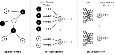
Figure 1: The aggregation and combination stages of GCN.

TABLE I: Structure and key features of the graph datasets and GCN configuration. Graphs are sorted based on the number of nodes (from left to right). In this paper, we explore an even mix of both small-scale (Corea/Citeseer/Pubmed/Flickr) and large-scale datasets (Reddit/Yelp/Pokec/Amazon) to highlight different effects GROW have as the scale of graph dataset is changed.

Datasets	Cora	Citeseer	Pubmed	Flickr	Reddit	Yelp	Pokec	Amazon
# of Nodes	2,708	3,327	19,717	89,250	232,965	716,847	1,632,803	2,449,029
# of Edges	13,264	12,431	108,365	989,006	114,848,857	13,954,819	46,236,731	126,167,309
Average degree	4.90	3.74	5.50	11.1	493	19.5	28.3	51.5
Feature length	1,433-16-7	3,703-16-6	500-16-3	500-64-7	602-64-41	300-64-100	60-64-48	100-64-47
Density of A	$1.81\times 10^{-3}$	$1.12\times 10^{-3}$	$2.79\times 10^{-4}$	$1.24\times 10^{-4}$	$2.12\times 10^{-3}$	$2.72\times 10^{-5}$	$1.73\times 10^{-5}$	$2.10\times 10^{-5}$
Density of $X^{(0)}$	1.27%	0.85%	10.0%	46.4%	100%	100%	39.9%	99.0%
Density of $X^{(1)}$	78.0%	89.1%	77.6%	77.2%	63.9%	77.2%	77.2%	77.2%
Density of W	100%	100%	100%	100%	100%	100%	100%	100%

II-B GCN as a Sparse-Dense GEMM Operation

A key computation pattern of a GCN layer is the two-stage matrix-multiplication, $A$$\times$$X$$\times$$W$. There are two possible execution orders: ($A$$\times$$X$)$\times$$W$ and $A$$\times$($X$$\times$$W$). Prior work on AWB-GCN [10] observed that the order in which $A$$\times$$X$$\times$$W$ is conducted has significant impact on the total number of MAC operations conducted. As shown in Table I, $A$ tends to be extremely large and sparse, $X$ being modestly sized and can be somewhat sparse but also be dense depending on the workload, and $W$ being small and highly dense. Consequently, adopting the ($A$$\times$$X$)$\times$$W$ execution order involves multiplying the sparse $A$ and sparse-or-dense $X$ first, producing a largely sized dense matrix, which is subsequently multiplied by another dense matrix $W$, leading to high computations. The alternative $A$$\times$($X$$\times$$W$) on the other hand can be handled as two consecutive sparse-dense matrix multiplications (SpDeGEMM) which can lead to smaller amount of computations (Figure 2) [44, 31]. Another important advantage of the aforementioned $A$$\times$($X$$\times$$W$) execution order is that the GCN layer can be handled with a single sparse-dense GEMM operation, making it possible to execute the two-stage SpDeGEMM end-to-end over a unified SpDeGEMM accelerator design.

II-C State-of-the-art Accelerators for GCN

HyGCN [44] is one of the first GCN accelerators that address the hybrid dataflow of both aggregation and combination. Specifically, HyGCN employs two separate engines, an aggregation engine optimized for the sparse-sparse GEMM of ($A$$\times$$X$) and a combination engine handling the subsequent dense-dense GEMM of ($AX$$\times$$W$). While HyGCN provides significant speedups vs. CPUs/GPUs, it falls short on two important aspects. First, one of the two engines in HyGCN can suffer from under-utilization due to load-imbalance. Second, as discussed in Section II-B, the execution order of ($A$$\times$$X$)$\times$$W$ can lead to a suboptimal dataflow with much higher computation demands than $A$$\times$($X$$\times$$W$), leaving significant performance left on the table.

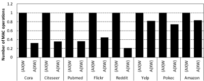
Figure 2: Normalized number of MAC operations depending on the execution order of two GEMMs, ($A$$\times$$X$)$\times$$W$ vs. $A$$\times$($X$$\times$$W$).

Consequently, AWB-GCN [10] employs the $A$$\times$($X$$\times$$W$) execution order of graph convolution, presenting a unified accelerator microarchitecture design. By permuting the two consecutive matrix multiplication operations into a SpDeGEMM operator, AWB-GCN achieves significant reduction in computational requirements with high speedups compared to HyGCN. More recently, GCNAX [31] introduces further dataflow optimizations on top of AWB-GCN using reconfigurable loop ordering, loop fusion, and efficient tiling strategies, achieving significant energy-efficiency improvements against both HyGCN and AWB-GCN. Given its robust accelerator design and state-of-the-art performance, the remainder of this paper assumes the $A$$\times$($X$$\times$$W$) execution order for GCN inference, using GCNAX as the baseline SpDeGEMM based GCN accelerator. Additionally, we henceforth refer to the $A$$\times$($XW$) as the aggregation phase and $X$$\times$$W$ as the combination phase for clarity of explanation.

III Related Work

TABLE II: Comparison between GROW and related work.

	GCNAX [31]	AWB-GCN [10]	HyGCN [44]	GAMMA [51]	Ours
Compute engine	Unified	Unified	Heterogeneous	Unified	Unified
Operend	Sp-De	Sp-De	Sp-De / De-De	Sp-Sp	Sp-De
Product type	Outer product	Inner product	Outer product / Inner product	Row-wise product	Row-wise product
Compress format	CSC	CSR	CSC	CSR	CSR
Preprocessing scheme	None	None	Graph partitioning / Vertex interval & edge sharding	Row Reordering & Coordinate-space tiling	HDN caching & graph partitioning

There is a large body of prior work that seek acceleration of sparse DNNs [1, 2, 23, 47, 48, 50, 19, 32, 38, 40, 10, 31, 44, 49, 22, 18, 42, 28, 27, 36, 26, 21, 25, 37, 35]. We summarize a subset of other related work in Table II that explores 1) alternative measures for accelerating GCNs, 2) locality-enhancing mechanisms for graph analytics, and 3) accelerator for sparse linear algebra.

Accelerating GCNs using ASIC/FPGA/GPU. Along with HyGCN [44], EnGN [32] is one of those first accelerators targeting GCNs, employing an output stationary dataflow with sequential pipelining to interleave the computation of aggregation and combination for high throughput. Cambricon-G [38] is another recent GCN accelerator employing a multi-dimensional cuboid engine. GRIP [23] is an accelerator based on the GReTA [22] programming abstraction whose architecture design and dataflow is similar to HyGCN. GraphACT [47] is a CPU-FPGA based accelerator targeting GCN training and GNNAdvisor [42] proposes an efficient software runtime system for GNN acceleration in GPUs. In general, the contribution of GROW is orthogonal to these prior work.

Techniques to enhance locality in graph analytics. Graph analytics are well-known for its irregular and sparse memory accesses exhibiting low locality. Consequently, several locality-enhancing solutions have been proposed in past literature for graph analytics (e.g., intelligent graph partitioning [20, 6], vertex reordering [52]). For instance, Zhang et al. [52] proposes a node degree-aware vertex reordering mechanism that helps improve locality for graph traversal algorithms. GROW builds upon these prior work to address the irregular reuse of dense matrices in GCN’s SpDeGEMM based inference, which we detail in Section V-C.

Accelerators for sparse linear algebra. Several recent studies explored the design of domain-specific architectures for sparse linear algebra. OuterSPACE [34] and SpArch [53] are two recent works that propose hardware accelerators for sparse-sparse GEMMs using an outer-product approach. ExTensor [14] is another recent study that applies the inner-product approach for sparse GEMMs. Tensaurus [40] is a versatile accelerator targeting both dense and sparse tensor factorizations. Most recently, MatRaptor [39] and GAMMA [51] explored the efficacy of utilizing Gustavson’s algorithm for accelerating sparse-sparse GEMMs. Similar to GROW, these two works employ a row-wise product based dataflow for minimizing data movements in this memory bandwidth limited algorithm, achieving significant energy-efficiency improvements. However, MatRaptor and GAMMA target generic sparse-sparse GEMM algorithms so it is not optimized to leverage the unique algorithmic properties of GCNs (e.g., the power-law distribution of graph datasets). Furthermore, the GCN we study is formulated as a sparse-dense GEMM, unlike the sparse-sparse GEMM these prior work focuses on. In Section VII-H, we quantitatively demonstrate GROW’s merits over both MatRaptor and GAMMA. Overall, the key contributions of GROW are orthogonal to these prior studies.

IV Motivation

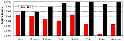
(a)

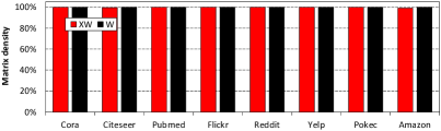
(b)

Figure 3: Density of (a) sparse matrices ($A$, $X$) and (b) dense matrices ($XW$, $W$) in the aggregation and combination stages.

IV-A Heterogeneous Levels of Sparsity in Graph Datasets

A key limitation of prior SpDeGEMM accelerators is that they do not exploit the different levels of sparsity manifested during aggregation and combination, simply treating them as a generic SpDeGEMM. Figure 3 illustrates the density of input matrices during aggregation and combination. First thing to note is that the right-hand side matrices (i.e., $XW$ in $A$$\times$$XW$ and $W$ in $X$$\times$$W$) of aggregation and combination are all extremely dense across all the graph datasets. However, the left-hand side matrices of the two SpDeGEMM operations (i.e., $A$ in $A$$\times$$XW$ and $X$ in $X$$\times$$W$) exhibit drastically different sparsity levels. That is, the sparse matrix in aggregation ($A$) is universally sparse with orders of magnitude higher sparsity than that of combination ($X$). The sparsity of matrix $X$, however, is mixed and oftentimes non-existent to begin with, i.e., highly dense for Reddit, Yelp, and Amazon.

Consequently, while the aggregation phase of GCN (i.e., $A$$\times$$XW$) can easily be generalized as a sparse-dense matrix multiplication, the combination phase can either be sparse-dense or dense-dense depending on the nature of the input feature vector, i.e., matrix $X$. Despite such heterogeneous and mixed levels of sparsity, however, the SpDeGEMM accelerator in GCNAX (as well as AWB-GCN) applies a rigid computational dataflow strictly tailored for the sparse-dense matrix multiplication for both aggregation and combination stages. We show that failing to incorporate such heterogeneous sparsity results in needless overprovisioning of on-chip buffers as well as significant waste in memory bandwidth.

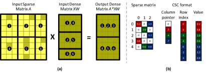
Figure 4: (a) GCNAX’s matrix tiling strategy for aggregation. The black numbered circles designate the order in which the input tiles are fetched (for $A$ and $XW$) and utilized for output tile derivation (for $A$$\times$$XW$). (b) The input sparse matrix is compressed in a CSC (compressed sparse column) format.

IV-B Tiling and Its Effect on On-/Off-chip Data Movement

Tiling matrices to temporarily store a subset of the active working set is a well-known, proven optimization strategy to reduce off-chip bandwidth requirement. Improving upon AWB-GCN’s tiling scheme, GCNAX proposes a dynamically reconfigurable loop unrolling and tiling mechanism, the high-level overview of which is provided in Figure 4. By carefully examining the two SpDeGEMM matrix shapes and graph dataset, GCNAX derives an optimal tile size for the sparse and dense matrices (tiled $A$ and tiled $XW$ in Figure 4(a)), which is utilized to derive the output tile based on an outer-product GEMM among the tile $A$ and tile $XW$. Note that the tiled sparse matrix is compressed in a CSC format (Figure 4(b)), which the GCNAX’s memory fetch unit utilizes to only fetch the non-zero elements within the currently working tile.

Our characterization reveals two important insights. First, GCNAX must provision the on-chip buffer size to be large enough to sufficiently capture the worst-case working set of sparse matrices $A$ and $X$. As discussed in Figure 3(a), however, matrix $X$ in several graph datasets are completely dense, so the size of the on-chip buffer must be (over)provisioned to match the exact size of GCNAX’s chosen tile size in the worst case that the input tile is completely dense. Because the density of matrix $A$ is extremely sparse, however, such overprovisioning of on-chip buffers are an extreme overkill during aggregation, wasting precious on-chip SRAM storage.

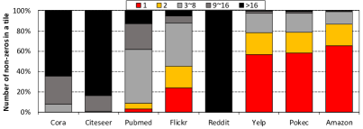
(a)

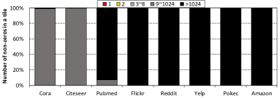
(b)

Figure 5: The number of non-zero elements within a tile in (a) matrix $A$ (aggregation) and (b) $X$ (combination).

Another important observation we make is that the number of non-zero elements manifested within a tile, for aggregation and combination, exhibits drastically different characteristics. Figure 5 summarizes the number of non-zero elements existent within the sparse tile fetched for GCNAX’s outer-product SpDeGEMM. During the combination stage, the number of non-zero elements within the tiled matrix $X$ are reasonably high, typically much more than $1024$ non-zeros per tile (Figure 5(b)). Such high density of non-zero elements enables a dense packing of effectual data within the compressed-sparse CSC format per each tile, achieving high memory bandwidth utilization when fetching the non-zero elements from the DRAM subsystem (the black bars in Figure 6). Unfortunately, the sparsity manifested during the aggregation stage exhibits a completely different pattern. As depicted in Figure 5(a), the adjacency matrix $A$ typically contains a very small number of non-zero elements (e.g., for Yelp/Pokec/Amazon, less than $3$ non-zero elements for more than $80\%$ of the tiles fetched from DRAM). Consequently, GCNAX’s effective memory bandwidth utilized for fetching effectual non-zero elements during aggregation becomes significantly low, averaging at $23\%$ (worst case $<$$6\%$) bandwidth utilization (the red bars in Figure 6). This is because the effectual non-zero elements within any given tile of matrix $A$ is typically much smaller than the minimum data access granularity of the DRAM subsystem (i.e., $64$ bytes), leading to a significant overfetch of useless data for the tiled SpDeGEMM. Given the memory bandwidth limited nature of sparse matrix multiplication operations [34, 53, 14], such significant waste in memory throughput renders the dataflow of GCNAX suboptimal, leaving significant performance left on the table. Overall, the performance of GCNAX gets completely bottlenecked by the low memory bandwidth utilization during the aggregation stage, spending significantly higher latency during aggregation than during the combination stage for large-scale graph datasets (Figure 7).

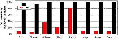
Figure 6: Effective memory bandwidth utilization when fetching the sparse matrices $A$ and $X$. Effective memory bandwidth utility is measured by counting how many bytes within the data read from DRAM are fetched on-demand assuming a $64$ byte minimum access granularity memory system.

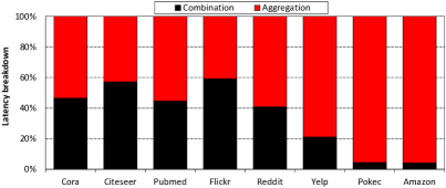
Figure 7: Breakdown of GCNAX’s end-to-end inference latency.

V GROW Architecture and Design

V-A Architecture Overview

GROW consists of a compute engine based on a vector processor, three sets of on-chip SRAM (I-BUF_sparse, I-BUF_dense, and O-BUF_dense) to maximize locality, a DMA unit that orchestrates on-/off-chip data movements, and the main control unit (Figure 8). The control unit populates the I-BUF_sparse and I-BUF_dense buffers with the sparse ($A$ and $X$) and dense ($XW$ and $W$) matrices of aggregation and combination stages and conducts the row-wise product based GEMM operation using vector processing, the output of which is stored into the O-BUF_dense in row granularity. The I-BUF_dense is functionally split into two subblocks, a high-degree node (HDN) cache that captures high locality dense matrix rows and a CAM (content addressable memory) based buffer that stores the list of top-$N$ high-degree node’s IDs. The sparse matrices $A$ and $X$ are compressed in CSR format while matrices $XW$ and $W$ are stored without compression in a dense fashion.

V-B Dataflow

A row-stationary dataflow for SpDeGEMM. Unlike GCNAX (or AWB-GCN) which employs an outer product (or inner product) based dataflow, GROW employs a row-wise product GEMM dataflow based on Gustavson’s algorithm [11] (Figure 9). In a row-wise product SpDeGEMM dataflow, all the non-zero elements from a single row of the left-hand side (LHS) matrix (the sparse, blue-colored elements) are multiplied with the non-zero elements from the corresponding rows of the right-hand side (RHS) matrix (the dense, green-colored elements), where the row index of the RHS matrix is determined by the column index of the non-zero values of LHS matrix. The results are accumulated into the corresponding row of the output matrix (the dense, red-colored elements). Because the $n$-th row in both the LHS matrix and the output matrix are all stationary during the course of row-wise product, we henceforth refer to this dataflow as row-stationary to differentiate it from a pure output-stationary dataflow [3].

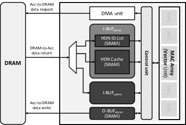
Figure 8: High-level overview of GROW.

A key advantage of a row-wise product is twofold. First, multiple rows from the output matrix can be computed in parallel as there are no data dependencies across different rows, allowing multiple processing engines to compute different rows of the output matrix without having to synchronize with each other. Because there are no dependencies across different rows, unlike the outer-product approach which mandates the entire ($2$D) input/output tiles to all be stored on-chip, row-wise product enables a design where several ($1$D) rows can be computed independently, allowing the required on-chip buffer space to store both the LHS matrix ($A$ and $X$) and the output matrix to be tuned to become relatively smaller than outer-product dataflow (yet with better utility). Such property helps better utilize memory bandwidth when fetching the active working set of the sparse matrix $A$. Figure 10 compares the number of non-zero (NZ) elements available for processing the SpDeGEMM when employing GCNAX’s 2D tiling strategy vs. GROW’s 1D row-wise product. As discussed in Section IV-B (Figure 5(a)), the number of non-zeros subject for SpDeGEMM within any given tile in GCNAX is typically less than $2$ in aggregation. GCNAX, however, fails to accommodate such sparsity patterns and applies a rigid 2D tiling window for both aggregation and combination. This leads to a significant waste in off-chip memory bandwidth because the number of effectual bytes (i.e., the number of non-zero elements within a given tile) fetched per $64$ bytes of minimum memory access granularity becomes small (Figure 10(b)). Contrast that with GROW’s row-stationary dataflow, where the number of effectual bytes fetched per memory access and utilized for SpDeGEMM is much higher and dense. This is because the CSR compression format compacts all the non-zero elements available within consecutive rows in a dense fashion (Figure 10(c)), all of which will be processed by our row-stationary SpDeGEMM computation within a short time window. Such alignment of CSR compressed effectual data of matrix $A$ and the row-wise product SpDeGEMM leads to much higher off-chip bandwidth utility as well as better on-chip buffer utilization.

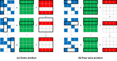
Figure 9: Outer-product vs. row-wise product GEMM dataflow..

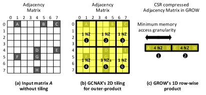
Figure 10: Difference between GCNAX’s 2D tiling for outer-product and GROW’s 1D row-wise product. The black numbered circles designate the order in which the input $2$D tile for (b) GCNAX or the $1$D row for (c) GROW is accessed for output derivation. (c) assumes the minimum memory access granularity is four elements wide.

Remaining challenges of row-stationary dataflow. Nonetheless, a critical trade-off made with the row-wise product (vs. inner-/outer-product) is that the RHS matrix ($XW$ and $W$) exhibits an irregular reuse across the derivation of different output rows, the locality of which is strictly dependent upon how the sparsity is manifested inside the LHS matrix (e.g., the $1$st row of the RHS matrix in Figure 9(b) is reused three times because there are three non-zero elements in the $1$st column of the LHS matrix). For the ($X$$\times$$W$) of combination stage, this is less of a concern as the weight matrix $W$ is typically small in GCNs, allowing it to be stored completely on-chip (Table I). Additionally, the fraction of execution time the combination stage accounts for is relatively small, especially for large-scale graph datasets (Figure 7). The aggregation stage ($A$$\times$$XW$), however, is a different story as the size of the RHS matrix $A$ scales proportional to the number of graph nodes, the number of which can amount to several millions and must be tiled across different iterations to be temporally stored on-chip. Such property renders an intelligent caching strategy that effectively balances both memory locality and parallelism crucial. In the following subsections, we detail our software/hardware co-design that maximizes locality (Section V-C) and parallelism (Section V-D) for high efficiency.

V-C Enhancing Locality via Graph Partitioning

The power-law distribution in real-world graphs. It is well known that real-world graphs in critical application domains follow the power-law distribution (Figure 11). Under the context of GCNs, this implies that only a small number of rows (or columns) within the adjacency matrix $A$ accounts for the majority of non-zeros while the remaining majority of rows (or columns) only contain a few non-zeros.

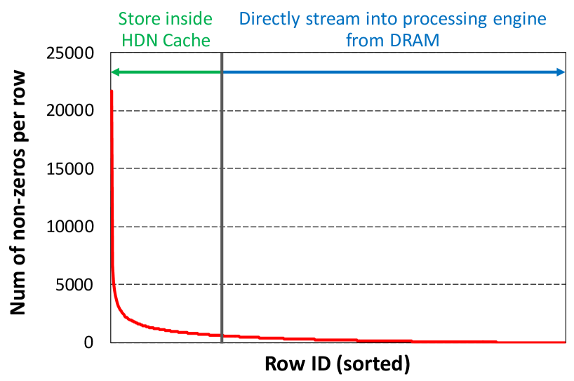
Figure 11: The power-law distribution of Reddit and how GROW utilizes that property for caching HDNs.

Our key approach is to utilize the power-law distribution of graph datasets to cost-effectively capture the (high) locality of those small number of HDN’s memory accesses. As discussed in Section V-A, the I-BUF_dense contains 1) an HDN cache that only captures the working set of high-degree node’s RHS matrix accesses during aggregation and 2) an HDN ID list buffer that stores the list of top-$N$ HDN’s IDs. Figure 12 illustrates an example of our approach, where nodes with ID$=$$0$,$3$,$4$ are determined as HDNs. The node IDs of the top-$N$ ($N=3$) high-degree nodes are stored as an array initially inside DRAM, which the DMA unit fetches and forwards to the I-BUF_dense controller so that it stores the HDN’s node ID information inside the HDN ID list buffer at the beginning of GCN inference (the details regarding how the node IDs of HDNs are derived are discussed later in this subsection). The I-BUF_dense controller subsequently fetches the corresponding HDN’s rows from the multiplicand matrix $XW$ and stores them inside the HDN cache. Once the (CSR compressed) non-zeros of the target row of the adjacency matrix $A$ is fetched inside I-BUF_sparse, the processing engine starts executing the SpDeGEMM, one row at a time (from the first to last row in Figure 12(b)). During the derivation of the first output row, the I-BUF_dense controller examines the HDN ID list buffer against the column IDs of the non-zero values of the first row of the adjacency matrix, finding out that three out of the five $XW$ row requests can be serviced from the HDN cache (i.e., the red-colored “H” (Hit) elements in the first row of Figure 12’s adjacency matrix). The controller therefore directly fetches the three HDN’s corresponding rows (ID$=$$0$,$3$,$4$) from the HDN cache while also requesting the DMA unit to stream in the (HDN cache missed) two low-degree node (LDN)’s rows (ID$=$$2$,$5$) from DRAM. Overall, once the HDN cache is populated with rows $0$,$3$,$4$, GROW can achieve a total of $13$ HDN cache hits while deriving the six output rows of $0-5$.

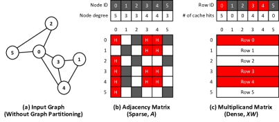
Figure 12: (a) Baseline input graph without graph partitioning and (b) its adjacency matrix. By only caching the top-$3$ high-degree nodes’ RHS multiplicand matrix accesses (c), a total of $13$ HDN cache hits is achieved.

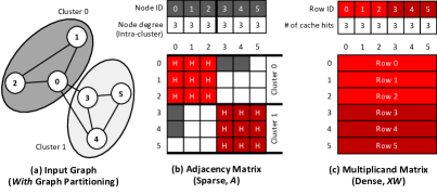
Figure 13: (a) Input graph with graph partitioning (target of $2$ partitions, resulting in three nodes per cluster) and (b) its adjacency matrix. Graph partitioning helps increase the number of HDN cache hits to $18$.

Graph partitioning to maximize temporal locality. As the HDN cache is designed to capture the locality of only the HDN nodes without accommodating the usage of LDN nodes, one could consider the HDN cache as a scratchpad for HDN nodes. When the input graph is small-scale, GROW’s scratchpad-like cache microarchitecture effectively exploits the graph’s power-law distribution, achieving high HDN cache hit rate (up to $80\%$ for Cora, Section VII-A) as well as significant speedup vs. GCNAX. Unfortunately, many real-world GCN applications like social network analysis or e-commerce are based on large-scale graph datasets, which contains an overwhelmingly large number of high-degree nodes for the statically sized HDN cache to sufficiently capture locality. As such, the effectiveness of GROW’s caching mechanism lies in how to intelligently utilize the limited HDN cache space to sufficiently capture the overall locality inherent in the adjacency matrix $A$ as a whole, regardless of its size.

To address such challenge, we use graph partitioning algorithms to partition the graph into multiple clusters, allowing GROW to achieve high intra-cluster temporal locality in GCN inference. Graph partitioning methods like Metis [20] or Graclus [6] are designed to construct the partitions over the input graph nodes such that intra-cluster nodes have much larger number of edges than inter-cluster nodes. In general, graph partitioning helps better capture the clustering and community structure of the graph and is a widely employed graph preprocessing technique for graph analytics. Figure 13 illustrates the effect of applying graph partitioning algorithm on the input graph of Figure 12(a). As depicted, graph partitioning only changes the way a particular node is assigned with its node ID (i.e., node ID is changed from $1\rightarrow 5$, $2\rightarrow 1$, and $5\rightarrow 2$ in Figure 13(a) vs. Figure 12(a)), yet the effect it has on the adjacency matrix is profound, especially for the purpose of GROW’s caching strategy. The key to our approach is to choose the top-N high-degree nodes subject for HDN caching only within the cluster, rather than across the entire adjacency matrix. Consider the example shown in Figure 13(b), where graph partitioning groups the non-zero values of cluster $0$ (node ID$=0$,$1$,$2$) in the upper-left corner of the adjacency matrix, while those of cluster $1$ are grouped at the lower-right corner (node ID$=3$,$4$,$5$). By tracking the top-$N$ HDN nodes per each cluster, GROW can cache nodes ID=$0$,$1$,$2$ (and ID=$3$,$4$,$5$) during the first (and second) cluster’s row-wise product based GEMM computation, leading to higher HDN cache hit rates than the baseline input graph. Figure 14 illustrates the effect of graph partitioning on a subset of our studied graph datasets, highlighting the several clusters of high-degree nodes around the diagonal line. In general, GROW’s HDN caching with graph partitioning is shown to achieve significant improvements in HDN cache hit rates (up to $17\times$ higher), which we quantify later in Section VII-A.

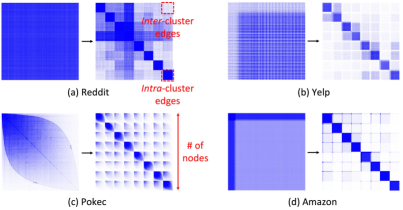
Figure 14: The effect of graph partitioning on the adjacency matrix of (a) Reddit, (b) Yelp, (c) Pokec, and (d) Amazon. For clear visualization, examples shown assume the graph partitioning algorithm targets $8$ output partitions, but our studied large-scale graphs are typically partitioned into thousands of clusters. Non-zero elements are colored in blue dots.

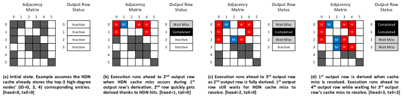
Figure 15: An example illustrating GROW’s multi-row stationary runahead execution mode.

Design overhead. Unlike the GCN input matrix $X$ whose value can change over different inputs, both the values as well as the structure of the adjacency matrix $A$ is statically fixed, regardless of what the GCN input is. Our proposal is to preprocess the adjacency matrix $A$ using graph partitioning, thereby generating multiple clusters of graph partitions with high temporal locality. Our software stack augments the Metis graph partitioning algorithm [20] with a pass that generates the top-$N$ high-degree nodes as a HDN ID list per each cluster, allowing the runtime hardware controller to fetch the HDN ID list before a target cluster begins computation. For a given target input graph, GROW’s graph preprocessing step incurs a one-time latency cost, as the partitioned graph and its HDN ID lists are used as-is for all future inference runs without modification. Consequently. the latency overheads of GROW graph preprocessing step (ranging from tens of milliseconds to several tens of minutes depending on the number of graph nodes) is amortized over all future GCN inference runs. In terms of storage overhead, the default GROW configuration employs a $12$ KB SRAM buffer within the I-BUF_dense in order to store the $4096$ HDN ID list of the current cluster (i.e., $4096$$\times$$3$B, $3$ Bytes per ID). The entire HDN ID lists for all the clusters per each graph amounts to several MBs of storage ($12$ KB per cluster, up to several thousands of clusters per graph) which is kept in DRAM.

V-D Enhancing Parallelism via Runahead Execution

Motivation. While GROW’s graph partitioning helps significantly reduce the number of HDN cache misses, the likelihood of any given output row’s derivation to incur a HDN cache miss is still high. We observe that, except for the small-scale Cora and Citeseer, an average $81\%$ of the output rows experience more than a single HDN cache miss per each row’s derivation (i.e., some of its HDN cache queries lead to hits while others result in misses). Having GROW actively work on just a single output row would therefore be highly suboptimal as the latency to service the HDN cache misses would directly be exposed to the processing engine, effectively blocking the derivation of other output rows and causing severe performance overheads.

Runahead execution with multi-row stationary dataflow. To address the aforementioned research challenge, GROW employs a multi-row stationary runahead execution scheme as means to maximize memory-level parallelism and hide the latency of HDN cache misses. The design objective of GROW’s multi-row stationary dataflow is to concurrently work on the derivation of multiple output rows, which is achieved by provisioning both the I-BUF_sparse and O-BUF_dense buffers to be large enough to keep track of multiple output rows’ derivation process. Figure 15 is an example of GROW multi-row stationary runahead execution assuming a $4$-way multi-row window (i.e., up to $4$ output rows can be actively worked upon by the processing engine) with node ID$=$$0$,$3$,$4$ determined as the HDN ID list. While executing the first output row, the GROW control unit experiences a HDN cache miss. Rather than idly waiting for the HDN cache miss to be resolved, the control unit runs ahead to the second row by fetching the second row’s (compressed) non-zero values of the adjacency matrix (Figure 15(b)). Because the two non-zero elements of $A$’s second row are all HDN cache hits, derivation of the second output row can be completed shortly while waiting for the first row’s cache miss to be serviced. Assuming the first row’s cache miss is not serviced in a timely manner, even though the second row has already completed its execution, GROW can keep running ahead to the third output row’s derivation (Figure 15(c)), further hiding the latency penalty of the first row’s HDN cache miss. While waiting for the third row’s cache miss to be resolved, GROW again runs ahead to the fourth row’s processing (Figure 15(d)), kicking off two more HDN cache misses inflight, maximizing memory-level parallelism and hiding its latency.

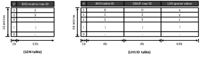
Figure 16: GROW microarchitectures enabling multi-row stationary runahead execution. The status of the two tables is updated assuming the same example shown in Figure 15, where LDN nodes with ID=$1$,$2$ miss in the HDN cache, allocating two entries inside the LDN table. Because output rows $0$, $2$, and $3$ requires RHS matrix rows of ID=$1$,$2$, this information is tracked inside the LHS ID table using three separate entries (the LHS sparse values to be multiplied with these three rows are assumed as $x$, $y$, $z$).

Implementation overhead. GROW’s runahead execution requires an MSHR (miss-status holding register) like microarchitecture that keeps track of which HDN cache queries have missed so far (i.e., LDN nodes) and are under the process of being fetched from the memory subsystem. Figure 16 provides a high-level overview of the key microarchitectural components that enable GROW’s runahead execution. First, an $M$ entry LDN table keeps track of the LDN nodes that missed in the HDN cache and is in need to fetch the missed RHS matrix rows from DRAM. Second, another $N$ entry LHS ID table stores the non-zero (sparse) LHS matrix values to be multiplied with the (HDN cache missed) RHS matrix rows. Once the missed RHS matrix row is fetched on-chip, the returned row’s corresponding table index ID allocated in the LDN table is used to conduct a CAM lookup inside the LHS ID table, allowing the corresponding O-BUF_dense to be updated properly. We empirically find that having these two tables be sized at $M=16$, $N=64$ sufficiently captures the benefits of runahead execution, amounting to $64$ Bytes (LDN table) and $544$ Bytes (LHS ID table) of storage space, respectively. Such design overhead is amortized over GROW’s several hundreds of KBs worth of on-chip SRAM capacity (detailed in Table IV).

VI Evaluation Methodology

Performance. We model both GCNAX and GROW as a cycle-level simulator implemented using C++. The simulator is driven by the studied graph datasets and the GCN input feature matrices (Table I) which we extracted using PyTorch Geometric [8], SNAP (Stanford Network Analysis Project) [30], and OGB (Open Graph Benchmark) [17]. For a fair comparison against state-of-the-art GCNAX, GROW has been configured to provide the same level of computation throughput and off-chip memory bandwidth while provisioned with similar on-chip SRAM capacity. Table III summarizes the key architectural parameters of GROW’s baseline configuration.

Area. We measure GROW’s area by implementing it in RTL using SystemVerilog. The RTL model is synthesized with Synopsys Design Compiler targeting $1$ GHz of operating frequency using a $65$ nm standard-cell library. The largest sized HDN cache is designed using $16$ banks of SRAM arrays, each array synthesized as a single-ported SRAM using a memory compiler. The fully associative HDN ID list is designed and synthesized as a CAM using D-flipflops for maximal performance, allowing a single cache lookup per each clock cycle. The small sized I-BUF_sparse and O-BUF_dense are implemented using dual-ported SRAMs and D-flipflops, respectively. GCNAX reports its area numbers under a $40$ nm technology, so we scale our area estimations from our $65$ nm results and report estimated numbers for $40$ nm when comparing against GCNAX (Table IV).

Energy. When quantifying energy consumption, we employ the energy model from [15] for quantifying energy per operation for both arithmetic operations as well as off-chip DRAM accesses. For modeling the power and energy consumption of on-chip SRAM usage, we use CACTI [16] targeting a $45$nm process. Since the area of both GCNAX and GROW is dominated by on-chip SRAM buffer space, we use CACTI’s leakage power to estimate static energy consumption.

TABLE III: GROW architecture configuration.

Parameter	Value
MAC width	$64$ bits
# MACs	$16$
I-BUFsparse	$12$ KB
HDN ID list	$12$ KB
HDN cache	$512$ KB
O-BUFdense	$2$ KB
Runahead execution degree	$16$
Memory bandwidth	$128$ GB/sec

TABLE IV: GROW vs. GCNAX area breakdown.

Component	Area ($mm^{2}$)
	$40$ nm	$40$ nm	$65$ nm
	(GCNAX)	$(estimated)$	$(measured)$
MAC array	-	0.232	0.613
I-BUFsparse	-	0.121	0.319
HDN ID list	-	0.421	1.112
HDN cache	-	1.352	3.569
O-BUFdense	-	0.043	0.113
Others	-	0.022	0.059
Total	6.51	2.191	5.785

VII Evaluation

VII-A Caching Efficiency and Memory Bandwidth Usage

Figure 17 compares GROW’s HDN cache hit rate with and without graph partitioning (denoted G.P). For small-scale graphs like Cora and Citeseer, the HDN cache is able to stash the majority of dense rows with high locality (all of the HDN cache misses are compulsory misses that the DMA unit brings on-chip immediately), leading to high HDN cache hit rate regardless of graph partitioning being employed. For large-scale graph datasets, however, graph partitioning provides substantial improvements in HDN hit rates (e.g., $5\%$$\rightarrow$$79\%$ for Amazon) which helps GROW dramatically reduce the off-chip memory traffic as illustrated in Figure 18. Reddit exhibits an unusually high average node degree (Table I, Figure 14(a)), which enables GCNAX to better exploit locality when conducting the $2$ planar tiled outer-product SpDeGEMM, having GROW incur $31\%$ higher memory traffic. Nonetheless, GROW with graph partitioning shows high robustness by significantly reducing off-chip memory accesses consistently across the other graph datasets, achieving $2\times$ (max $4.7\times$) reduction in DRAM traffic vs. GCNAX.

To better isolate the effect of HDN caching with graph partitioning, we also show in Figure 19 the memory traffic reduction achieved with and without HDN caching and graph partitioning. GROW without HDN caching and graph partitioning incurs a significantly higher DRAM burden, incurring an average $4.3\times$ higher memory traffic than GROW with HDN caching but without graph partitioning ($5.8\times$ higher traffic than GROW with both HDN caching and graph partitioning).

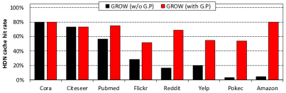
Figure 17: HDN cache hit rate with and without graph partitioning (G.P). Caching without graph partitioning simply caches the top-$N$ (=$4096$) high-degree nodes.

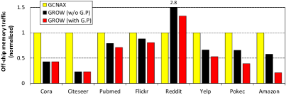
Figure 18: Total number of bytes read from DRAM (normalized to GCNAX).

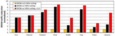
Figure 19: The effect of HDN caching and graph partitioning on GROW’s DRAM traffic reduction (normalized to GROW without HDN caching and graph partitioning). The higher the better.

VII-B Performance

GROW significantly improves the performance of GCNs, especially for the large-scale and sparse graph datasets, achieving an average $2.8\times$ speedup (max $14.2\times$) vs. GCNAX. It is worth pointing out that the bulk of GROW’s performance benefits comes from greatly reducing the latency spent in conducting the aggregation stage. As discussed in Figure 7, GCNAX spends significant fraction of execution time in the aggregation stage, especially for the large-scale graphs like Yelp, Pokec, and Amazon. As depicted in Figure 20(b), GROW successfully reduces the latency in this critical bottleneck stage by an average $6.3\times$, shifting the GCN inference bottleneck now to the combination stage.

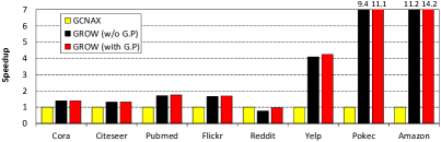
(a)

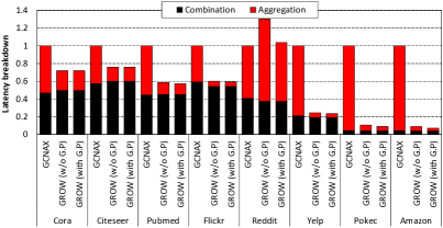
(b)

Figure 20: (a) GROW speedup vs. GCNAX and (b) a latency breakdown (normalized to GCNAX).

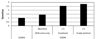
Figure 21: GROW’s average speedup when incrementally applying our proposed optimizations one-by-one (from left to right).

VII-C Ablation Study

To clearly demonstrate where GROW’s speedup comes from, we quantify the impact of isolating our three main proposals in Figure 21 as an ablation study. The baseline GROW employs the proposed row-stationary dataflow with HDN caching but without runahead execution nor graph partitioning, achieving an average $1.4\times$ speedup. Applying runahead execution provides a further $1.8\times$ speedup, with graph partitioning additionally reducing latency by $1.1\times$.

VII-D Energy-Efficiency

Figure 22 shows a breakdown of energy consumption in GCNAX and the two design points of our GROW architecture. Given the memory bound nature of SpDeGEMM, a large portion of dynamic energy is consumed in off-chip data movements rather than on-chip SRAM accesses or compute. Thanks to the significant reduction in memory traffic, GROW noticeably reduces energy consumed in off-chip memory accesses. Additionally, GROW also significantly reduces static energy consumption thanks to the reduction in execution time, achieving an overall $2.3\times$ improvement in energy-efficiency.

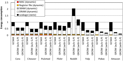
Figure 22: Energy consumption of GROW (normalized to GCNAX).

VII-E Area Analysis

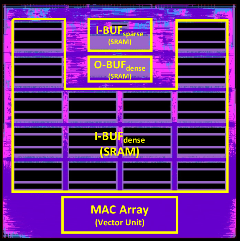
Figure 23: GROW layout.

The total area of GROW is $5.8$mm² synthesized with a $65$ nm standard-cell library (Table IV). The majority of area is used by the on-chip SRAM buffers ($88\%$), especially the I-BUF_dense buffer (i.e., HDN cache and HDN ID list), which is a good design point to pursue as sparse SpDeGEMM algorithms are typically bottlenecked on off-chip memory bandwidth.

The area of GCNAX is reported as $6.5$mm² synthesized under a $40$ nm technology. When GROW’s area is scaled down to $40$ nm, its area is estimated as $2.2$mm². Given GROW’s superior performance and energy-efficiency, GROW provides an average $8.2\times$ better performance/mm² numbers. Figure 23 shows the final placed-and-routed design layout of GROW.

VII-F Scalability

Figure 24 shows GROW’s performance when the number of processing engines (PEs) are swept from $1$ PE to $16$ PEs with a proportional increase in memory bandwidth. For small-scale graphs like Cora and Citeseer, having just a single GROW PE is sufficient to capture the entire working set, so the benefits of larger number of PEs are small. As the input graph gets larger, however, the benefit of GROW’s fine-grained row-stationary dataflow shines, achieving high scalability. In fact, for large-scale graphs like Yelp, Pokec and Amazon, GROW achieves a super-linear speedup. We observe that different PEs exhibit different memory intensive phases at different times as each PE handles a different graph cluster containing different loads. This leads to certain periods where a given PE is artificially given more than the average unit memory bandwidth (i.e., the memory bandwidth a single PE is provided with on average assuming perfect load balancing at steady state), which helps increase performance further.

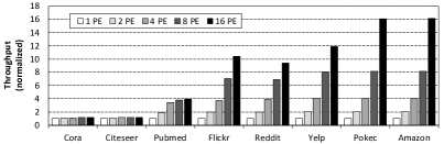
Figure 24: Performance scalability as a function of the number of PEs.

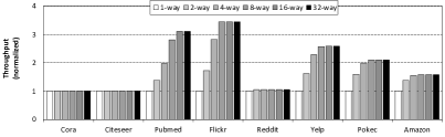
(a)

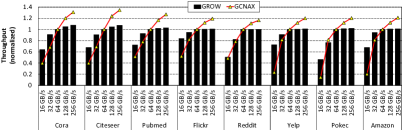
(b)

Figure 25: GROW sensitivity study. (a) Performance of GROW when changing the degree of runahead execution. (b) Normalized performance of GCNAX and GROW when changing the off-chip memory bandwidth, from $16$ GB/sec to $256$ GB/sec. In (b), note that both GCNAX and GROW are each normalized to its own $64$ GB/sec design point in order to show the accelerator’s sensitivity to memory bandwidth (i.e., the slope of GCNAX is much more steep than GROW, meaning GCNAX suffers more from SpDeGEMM’s memory bandwidth limited characteristics).

VII-G Sensitivity

Runahead execution degree. Figure 25(a) shows the performance of GROW as we sweep the runahead execution degree from $1$$-$$32$-ways. In five out of the eight workloads we study, there is a sizable performance gap between $1$-way and $8$/$16$-way runahead execution mode, demonstrating the importance of optimizing GROW memory-level parallelism using our multi-row stationary dataflow.

Off-chip memory bandwidth. Figure 25(b) shows the changes in GCNAX and GROW’s throughput when the memory bandwidth is swept from $16$ to $256$ GB/sec. Both GCNAX and GROW are each normalized to its own performance with $64$ GB/sec memory bandwidth as means to highlight its robustness under different levels of memory throughput provided. As depicted, GCNAX is highly sensitive to memory bandwidth showing a sharp increase (decrease) in performance when the provided memory bandwidth is increased (decreased). In contrast, GROW shows high robustness in performance thanks to its better utilization of memory bandwidth.

VII-H Comparison to MatRaptor and GAMMA

While the row-wise product based MatRaptor [39] and GAMMA [51] do not explore GCNs nor target sparse-dense GEMM as in GROW, given their adoption of Gustavson’s algorithm, we implement a cycle-level simulator of both MatRaptor/GAMMA to demonstrate GROW’s merits. In Figure 26, GROW provides an average $9.3\times$/$1.5\times$ speedup vs. MatRaptor/GAMMA, respectively. Reasons for GROW’s speedup are threefold. First, MatRaptor/GAMMA are optimized for generic sparse-sparse GEMM so they fail to effectively exploit GCN-inherent locality, i.e., MatRaptor does not employ caches and GAMMA’s fiber cache is not optimized for the power-law distribution of graphs. Second, sparse-sparse GEMM incurs a complicated and costly partial-sum merging process, which is entirely redundant for SpDeGEMM (i.e., key primitive of GROW is a scalar $\times$ vector operation, Figure 9(b)), only to add performance and area overheads. Third, the sparse-sparse GEMM assumes the RHS matrix is compressed in CSR which adds additional indexing overheads as well as more memory traffic to fetch metadata associated with CSR. On average, GROW reduces memory traffic by an average $18\times$/$4\times$ (maximum $46\times$/$7\times$) vs. MatRaptor/GAMMA, respectively, leading to high speedup.

VIII Discussion

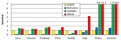
Figure 26: Performance comparison of GROW vs. MatRaptor/GAMMA.

GROW for non-power-law graphs. As the efficiency of graph partitioning is dependent upon the power-law distribution of input graphs, the effectiveness of GROW’s HDN caching will be reduced for non-power-law graphs. Nonetheless, we expect the abundant parallelism reaped out by the combination of GROW’s row-stationary dataflow and runahead execution to better hide latency than GCNAX, maintaining its superiority for even these challenging input datasets. Evaluation of GROW for such graphs however is beyond the scope of this paper and we leave it as future work.

Pinned vs. demand-based cache replacement policy. While GROW employs a policy where high-degree nodes are “pinned” inside the HDN cache, we also experimented with alternative cache eviction/replacement policies. For instance, we also considered cache designs that seek to better capture locality for low-degree nodes (e.g., the higher priority high-degree node cache entries can get evicted to store low-degree nodes per LRU policy) but it turns out that statically pinning the high-degree nodes within the cache (as our current proposition) yielded the most robust speedups. This is because the opportunity loss of evicting a high-degree node greatly outweighed the benefits of capturing low-degree node’s locality.

GROW applicability for advanced aggregation functions. Here we discuss GROW’s applicability for more advanced aggregation functions discussed in prior work. SAGEConv [8] employs an aggregation function which conducts either a mean, pool, or LSTM operation over the sampled neighbor nodes  [13]. Using the sampled node ID list, GROW’s row-stationary dataflow can naturally fetch the sampled nodes from the $X$ matrix, which then goes through mean, pool, or LSTM. Unlike the mean/LSTM operators which GROW’s existing microarchitecture (e.g., MAC array) can readily be employed for derivation, pooling requires a separate, vector comparator array for accelerated computation. When implemented and synthesized with $65$ nm standard-cell library, such comparator array incurs $1.4\%$ additional area overhead vs. current GROW design. GIN [43] employs an aggregation function which adjusts the weight of the central node using a learnable parameter. As discussed in GCNAX, such aggregation function is refactored into multiple consecutive $W$ matrices so GROW is fully capable of supporting GIN as-is. GAT [41] utilizes attention layers as its aggregation function, which involves MLP and softmax operators. While MLPs can be computed using GROW’s MAC array, derivation of softmax requires additional microarchitectural support. There are multiple prior literature discussing hardware-accelerated softmax design (e.g., approximated polynomial based [33] vs. hash-table based [12]), the most optimal design decision governed by the distribution of the values subject for softmax operation. Prior work on $A^{3}$ [12] reports that a high-overhead table-based softmax accelerator incurs approximately $16\%$ additional area overhead vs. its MAC array. When conservatively projecting similar overheads to GROW’s MAC array design, supporting GAT is estimated to incur a chip-wide $1.7\%$ area overhead. We leave the evaluation of GROW for these aggregation functions as future work as it is beyond the scope of this paper.

IX Conclusion

This paper presents a GCN inference accelerator named GROW based on the Gustavson’s algorithm. GROW is based on our software and hardware co-design which effectively balances locality and parallelism for high performance. Unlike prior SpDeGEMM based GCN accelerators, GROW is capable of intelligently exploiting the heterogeneous sparsity levels manifested during the aggregation and combination phases of GCNs, drastically reducing memory traffic for the memory-bound SpDeGEMM algorithm. Compared to state-of-the-art GCNAX, GROW reduces memory traffic by $2\times$, and achieves an average $2.8\times$, $2.3\times$, and $8.2\times$ improvement in performance, energy-efficiency, and performance/area, respectively.

References

- [1] S. Abadal, A. Jain, R. Guirado, J. López-Alonso, and E. Alarcón, “Computing Graph Neural Networks: A Survey from Algorithms to Accelerators,” Computing Surveys (CSUR), 2021.
- [2] A. Auten, M. Tomei, and R. Kumar, “Hardware Acceleration of Graph Neural Networks,” in Design Automation Conference (DAC), 2020.
- [3] Y.-H. Chen, T. Krishna, J. S. Emer, and V. Sze, “Eyeriss: An Energy-efficient Reconfigurable Accelerator for Deep Convolutional Neural Networks,” in Proceedings of the International Solid State Circuits Conference (ISSCC), 2016.
- [4] H. Dai, Z. Kozareva, B. Dai, A. Smola, and L. Song, “Learning Steady-States of Iterative Algorithms over Graphs,” in In ICML. 1114-1122, 2018.
- [5] N. De Cao and T. Kipf, “MolGAN: An Implicit Generative Model for Small Molecular Graphs,” in arXiv.org, 2018.
- [6] I. Dhillon, Y. Guan, and B. Kulis, “A Fast Kernel-Based Multilevel Algorithm for Graph Clustering,” in Proceedings of the International Conference on Knowledge Discovery & Data Mining (KDD), 2005.
- [7] D. Duvenaud, D. Maclaurin, J. Aguilera-Iparraguirre, R. GomezBombarelli, T. Hirzel, A. Aspuru-Guzik, and R. P. Adams, “Convolutional Networks on Graphs for Learning Molecular Fingerprints,” in In Proceedings of the International Conference on Neural Information Processing Systems (NIPS), 2015.
- [8] M. Fey and J. E. Lenssen, “Fast Graph Representation Learning with PyTorch Geometric,” in arXiv.org, 2019.
- [9] A. Fout, J. Byrd, B. Shariat, and A. Ben-Hur, “Protein Interface Prediction Using Graph Convolutional Networks,” in In Proceedings of the International Conference on Neural Information Processing Systems (NIPS), 2017.
- [10] T. Geng, A. Li, R. Shi, C. Wu, T. Wang, Y. Li, P. Haghi, A. Tumeo, S. Che, S. Reinhardt et al., “AWB-GCN: A Graph Convolutional Network Accelerator with Runtime Workload Rebalancing,” in Proceedings of the International Symposium on Microarchitecture (MICRO), 2020.
- [11] F. G. Gustavson, “Two Fast Algorithms for Sparse Matrices: Multiplication and Permuted Transposition,” ACM Transactions on Mathematical Software (TOMS), 1978.
- [12] T. J. Ham, S. J. Jung, S. Kim, Y. H. Oh, Y. Park, Y. Song, J.-H. Park, S. Lee, K. Park, J. W. Lee, and D.-K. Jeong, “A3: Accelerating Attention Mechanisms in Neural Networks with Approximation,” in Proceedings of the International Symposium on High-Performance Computer Architecture (HPCA), 2020.
- [13] W. L. Hamilton, R. Ying, and J. Leskovec, “Inductive Representation Learning on Large Graphs,” in Proceedings of the International Conference on Neural Information Processing Systems (NIPS), 2017.
- [14] K. Hegde, H. Asghari-Moghaddam, M. Pellauer, N. Crago, A. Jaleel, E. Solomonik, J. Emer, and C. W. Fletcher, “ExTensor: An Accelerator for Sparse Tensor Algebra,” in Proceedings of the International Symposium on Microarchitecture (MICRO), 2019.
- [15] M. Horowitz, “Computing’s Energy Problem (and What We Can Do About It),” in Proceedings of the International Solid State Circuits Conference (ISSCC), 2014.
- [16] HP Labs, “CACTI: An Integrated Cache and Memory Access Time, Cycle Time, Area, Leakage, and Dynamic Power Model,” http://www.hpl.hp.com/research/cacti/, 2016.
- [17] W. Hu, M. Fey, M. Zitnik, Y. Dong, H. Ren, B. Liu, M. Catasta, and J. Leskovec, “Open Graph Benchmark: Datasets for Machine Learning on Graphs,” in arXiv.org, 2020.
- [18] G. Huang, G. Dai, Y. Wang, and H. Yang, “GE-SpMM: General-Purpose Sparse Matrix-Matrix Multiplication on GPUs for Graph Neural Networks,” in Proceedings of the International Conference on High Performance Computing, Networking, Storage and Analysis (SC), 2020.
- [19] R. Hwang, T. Kim, Y. Kwon, and M. Rhu, “Centaur: A Chiplet-based, Hybrid Sparse-Dense Accelerator for Personalized Recommendations,” in Proceedings of the International Symposium on Computer Architecture (ISCA), 2020.
- [20] G. Karypis and V. Kumar, “A Fast and High Quality Multilevel Scheme for Partitioning Irregular Graphs,” SIAM Journal on scientific Computing, 1998.
- [21] B. Kim, J. Park, E. Lee, M. Rhu, and J. H. Ahn, “TRiM: Tensor Reduction in Memory,” in IEEE Computer Architecture Letters, 2020.
- [22] K. Kiningham, P. Levis, and C. Ré, “GReTA: Hardware Optimized Graph Processing for GNNs,” in Proceedings of the Workshop on Resource-Constrained Machine Learning (ReCoML), 2020.
- [23] K. Kiningham, C. Re, and P. Levis, “GRIP: A Graph Neural Network Accelerator Architecture,” arXiv.org, 2020.
- [24] T. N. Kipf and M. Welling, “Semi-Supervised Classification with Graph Convolutional Networks,” in Proceedings of the International Conference on Learning Representations (ICLR), 2017.
- [25] Y. Kwon, Y. Lee, and M. Rhu, “TensorDIMM: A Practical Near-memory Processing Architecture for Embeddings and Tensor Operations in Deep Learning,” in Proceedings of the International Symposium on Microarchitecture (MICRO), 2019.
- [26] Y. Kwon, Y. Lee, and M. Rhu, “Tensor Casting: Co-designing Algorithm-architecture for Personalized Recommendation Training,” in Proceedings of the International Symposium on High-Performance Computer Architecture (HPCA), 2021.
- [27] Y. Kwon and M. Rhu, “Training Personalized Recommendation Systems from (GPU) Scratch: Look Forward Not Backwards,” in Proceedings of the International Symposium on Computer Architecture (ISCA), 2022.
- [28] Y. Lee, J. Chung, and M. Rhu, “SmartSAGE: Training Large-scale Graph Neural Networks using In-Storage Processing Architectures,” in Proceedings of the International Symposium on Computer Architecture (ISCA), 2022.
- [29] A. Lerer, L. Wu, J. Shen, T. Lacroix, L. Wehrstedt, A. Bose, and A. Peysakhovich, “Pytorch-BigGraph: A Large-Scale Graph Embedding System,” in arXiv.org, 2019.
- [30] J. Leskovec and A. Krevl, “SNAP Datasets: Stanford Large Network Dataset Collection,” http://snap.stanford.edu/data, Jun. 2014.
- [31] J. Li, A. Louri, A. Karanth, and R. Bunescu, “GCNAX: A Flexible and Energy-Efficient Accelerator for Graph Convolutional Neural Networks,” in Proceedings of the International Symposium on High-Performance Computer Architecture (HPCA), 2021.
- [32] S. Liang, Y. Wang, C. Liu, L. He, L. Huawei, D. Xu, and X. Li, “EnGN: A High-Throughput and Energy-Efficient Accelerator for Large Graph Neural Networks,” IEEE Transactions on Computers, 2020.
- [33] A. Marchisio, B. Bussolino, E. Salvati, M. Martina, G. Masera, and M. Shafique, “Enabling Capsule Networks at the Edge through Approximate Softmax and Squash Operations,” in Proceedings of the ACM/IEEE International Symposium on Low Power Electronics and Design, 2022.
- [34] S. Pal, J. Beaumont, D.-H. Park, A. Amarnath, S. Feng, C. Chakrabarti, H.-S. Kim, D. Blaauw, T. Mudge, and R. Dreslinski, “OuterSPACE: An Outer Product Based Sparse Matrix Multiplication Accelerator,” in Proceedings of the International Symposium on High-Performance Computer Architecture (HPCA), 2018.
- [35] A. Parashar, M. Rhu, A. Mukkara, A. Puglielli, R. Venkatesan, B. Khailany, J. Emer, S. W. Keckler, and W. J. Dally, “SCNN: An Accelerator for Compressed-sparse Convolutional Neural Networks,” in Proceedings of the International Symposium on Computer Architecture (ISCA), 2017.
- [36] J. Park, B. Kim, S. Yun, E. Lee, M. Rhu, and J. H. Ahn, “TRiM: Enhancing Processor-Memory Interfaces with Scalable Tensor Reduction in Memory,” in Proceedings of the International Symposium on Microarchitecture (MICRO), 2021.
- [37] M. Rhu, M. O’Connor, N. Chatterjee, J. Pool, Y. Kwon, and S. W. Keckler, “Compressing DMA Engine: Leveraging Activation Sparsity for Training Deep Neural Networks,” in Proceedings of the International Symposium on High-Performance Computer Architecture (HPCA), 2018.
- [38] X. Song, T. Zhi, Z. Fan, Z. Zhang, X. Zeng, W. Li, X. Hu, Z. Du, Q. Guo, and Y. Chen, “Cambricon-G: A Polyvalent Energy-efficient Accelerator for Dynamic Graph Neural Networks,” IEEE Transactions on Computer-Aided Design of Integrated Circuits and Systems, 2021.
- [39] N. Srivastava, H. Jin, J. Liu, D. Albonesi, and Z. Zhang, “MatRaptor: A Sparse-Sparse Matrix Multiplication Accelerator Based on Row-Wise Product,” in Proceedings of the International Symposium on Microarchitecture (MICRO), 2020.
- [40] N. Srivastava, H. Jin, S. Smith, H. Rong, D. Albonesi, and Z. Zhang, “Tensaurus: A Versatile Accelerator for Mixed Sparse-Dense Tensor Computations,” in Proceedings of the International Symposium on High-Performance Computer Architecture (HPCA), 2020.
- [41] P. Veličković, G. Cucurull, A. Casanova, A. Romero, P. Lio, and Y. Bengio, “Graph Attention Networks,” in Proceedings of the International Conference on Learning Representations (ICLR), 2018.
- [42] Y. Wang, B. Feng, G. Li, S. Li, L. Deng, Y. Xie, and Y. Ding, “GNNAdvisor: An Adaptive and Efficient Runtime System for GNN Acceleration on GPUs,” in Proceedings of the International Symposium on Operating Systems Design and Implementation (OSDI), 2021.
- [43] K. Xu, W. Hu, J. Leskovec, and S. Jegelka, “How Powerful are Graph Neural Networks?” in arXiv.org, 2018.
- [44] M. Yan, L. Deng, X. Hu, L. Liang, Y. Feng, X. Ye, Z. Zhang, D. Fan, and Y. Xie, “HyGCN: A GCN Accelerator with Hybrid Architecture,” in Proceedings of the International Symposium on High-Performance Computer Architecture (HPCA), 2020.
- [45] H. Yang, “AliGraph: A Comprehensive Graph Neural Network Platform,” in Proceedings of the International Conference on Knowledge Discovery & Data Mining (KDD), 2019.
- [46] R. Ying, J. You, C. Morris, X. Ren, W. L. Hamilton, and J. Leskovec, “Hierarchical Graph Representation Learning with Differentiable Pooling,” in In Proceedings of the International Conference on Neural Information Processing Systems (NIPS), 2018.
- [47] H. Zeng and V. Prasanna, “GraphACT: Accelerating GCN Training on CPU-FPGA Heterogeneous Platforms,” in Proceedings of the ACM International Symposium on Field-Programmable Gate Arrays (FPGA), 2020.
- [48] H. Zeng, H. Zhou, A. Srivastava, R. Kannan, and V. Prasanna, “Graphsaint: Graph Sampling Based Inductive Learning Method,” in Proceedings of the International Conference on Learning Representations (ICLR), 2020.
- [49] B. Zhang, R. Kannan, and V. Prasanna, “BoostGCN: A Framework for Optimizing GCN Inference on FPGA,” in Proceedings of the International Symposium on Field-Programmable Custom Computing Machines (FCCM), 2021.
- [50] B. Zhang, H. Zeng, and V. Prasanna, “Hardware Acceleration of Large Scale GCN Inference,” in Proceedings of the International Conference on Application-specific Systems, Architectures and Processors (ASAP), 2020.
- [51] G. Zhang, N. Attaluri, J. S. Emer, and D. Sanchez, “GAMMA: Leveraging Gustavson’s Algorithm to Accelerate Sparse Matrix Multiplication,” in Proceedings of the International Conference on Architectural Support for Programming Languages and Operation Systems (ASPLOS), 2021.
- [52] J. Zhang and J. Li, “Degree-aware Hybrid Graph Traversal on FPGA-HMC Platform,” in Proceedings of the ACM International Symposium on Field-Programmable Gate Arrays (FPGA), 2018.
- [53] Z. Zhang, H. Wang, S. Han, and W. J. Dally, “SpArch: Efficient Architecture for Sparse Matrix Multiplication,” in Proceedings of the International Symposium on High-Performance Computer Architecture (HPCA), 2020.