Functional reduction of one-loop Feynman integrals with arbitrary masses

O.V. Tarasov

Joint Institute for Nuclear Research,
141980 Dubna, Russian Federation
E-mail: otarasov@jinr.ru

A method of functional reduction for the dimensionally regularized one-loop Feynman integrals with massive propagators is described in detail.

The method is based on a repeated application of the functional relations proposed by the author. Explicit formulae are given for reducing one-loop scalar integrals to a simpler ones, the arguments of which are the ratios of polynomials in the masses and kinematic invariants. We show that a general scalar $n$-point integral, depending on $n(n+1)/2$ generic masses and kinematic variables, can be expressed as a linear combination of integrals depending only on $n$ variables. The latter integrals are given explicitly in terms of hypergeometric functions of $(n-1)$ dimensionless variables. Analytic expressions for the 2-, 3- and 4-point integrals, that depend on the minimal number of variables, were also obtained by solving the dimensional recurrence relations. The resulting expressions for these integrals are given in terms of Gauss’ hypergeometric function ${}_{2}F_{1}$, the Appell function $F_{1}$ and the hypergeometric Lauricella - Saran function $F_{S}$. A modification of the functional reduction procedure for some special values of kinematical variables is considered.

1 Introduction

Feynman integrals play an important role in making precise perturbative predictions in quantum field theory and statistical physics. Theoretical predictions for experiments at the LHC [1, 2] as well as at future colliders such as the FCC [3] demand knowledge of precise radiative corrections. Precise experimental measurements are to be interpreted with sufficient precision of theoretical predictions [4]. The complexity of the evaluation of such radiative corrections is related, in particular, to the difficulties in calculating integrals corresponding to Feynman diagrams with many external legs depending on many kinematical variables. Purely numerical evaluation of such integrals sometimes cannot provide sufficiently high precision within reasonable computer time. Problems of numerical evaluation of the one-loop integrals have been considered, for example, in refs. [5], [6], [7], [8]. Numerical instability in evaluating one-loop scalar integrals near exceptional momentum configurations was addressed in refs. [9], [10], [11].

At present, there are many various methods of evaluating Feynman integrals. Some methods are based on the fact that these integrals are functions of continuous variables - scalar products of external momenta and masses, and are also functions of discrete parameters - powers of propagators as well as space - time dimension parameter $d$. External kinematic invariants and squared masses were used to derive differential equations [12] (see also reviews [13], [14]). Space-time dimension $d$ and powers of propagators were used to derive difference equations [15], [16], [17] for these integrals. Then the results for integrals are obtained by solving these equations. Practical application of the method of differential equation and methods based on recurrence relations to evaluating high-order, multi-leg Feynman diagrams, clearly demonstrate the need for further improvements and development of methods for solving differential and recursion relations.

On the other hand, it is possible to extend the applicability of these methods by combining them with other approaches. For instance, these methods can be used in combination with approach proposed in refs. [18], [19], [20]. In ref. [18], a new type of relations between Feynman integrals, namely functional relations has been discovered. In ref. [19] a simple method has been proposed for deriving functional relations applicable to integrals corresponding to Feynman diagrams with any number of loops and legs. Using these relations a method of functional reduction was formulated and applied to several massless integrals in ref. [20]. This method allows one to express the integral of interest in terms of integrals with fewer variables. In general, the latter integrals will be easier to evaluate by the above mentioned methods than the original integral.

Integrals appearing in the final results of functional reduction have two important features. Firstly, that they depend on the minimal number of variables (MNV) and, secondly, these variables are the ratios of Gram determinants.

As for our representation of integrals in terms of functions that depend explicitly on ratios of the Gram determinants, we would like to mention refs. [6],[11] where the importance of representing kinematic dependence of integrals in terms of ratios of the Gram determinants was demonstrated. As the authors have shown, such a representation turns out to be useful for the stability of numerical calculation of integrals.

The primary purpose of the paper is to apply the method of functional reduction to the scalar one - loop integrals that depend on arbitrary kinematic variables and masses.

The article is organized as follows. In Section 2, we will briefly describe the method for deriving functional relations given in ref. [19]. In Section 3, we describe the method of functional reduction proposed in ref. [20]. In Section 4, the functional reduction of the 2-point integral is considered. In Section 5, a two-step functional reduction of the integral corresponding to a 3-point Feynman diagram is described. The Feynman parameter representation and dimensional recurrence relations for the integrals arising at the final stage of the functional reduction are given. We present an analytic result derived by a use of the dimensional recurrence relation as well as a result in terms of a double hypergeometric series, obtained by expanding the Feynman parameter integral.

In Section 6, we propose three-step functional reduction procedure for the 4-point integral. Solving the dimensional recurrence relation, we obtained an analytic result for the integral depending on the MNV. Also, representation of this integral in terms of a triple hypergeometric series is given.

In Section 7, we describe derivation of functional relations of a four-step reduction procedure for the 5-point integral. We also give here the Feynman parameter representation of the 5-point integral depending on the MNV as well as a dimensional recurrence relation for this integral. Using a parametric representation of the integral, we expressed it as a fourfold hypergeometric series.

In Section 8, we describe 5 steps of the functional reduction of a 6-point integral. The Feynman parameter representation and a dimensional recurrence relation for the integral with the MNV are given. Using a parametric representation, we expressed the integral as a multiple hypergeometric series.

In Section 9, we describe a modification of the functional reduction method for integrals depending on special values of kinematical variables and present analytic results for these integrals.

In Section 10, a general method is proposed for obtaining the final formula of the functional reduction for an arbitrary one-loop $n$ - point integral. A parametric representation is also given for the $n$-point integrals depending on the MNV. Using this parametric representation, we obtain a representation of the integral in terms of multiple hypergeometric series.

We offer some concluding remarks in Section 11. Finally in the Appendix, we give formulae for kinematic determinants and hypergeometric functions that were used in our paper.

2 Algebraic relation between propagators

We consider one-loop scalar integral in general dimension $d$ corresponding to a Feynman diagram with $n$ external lines and $n$ internal propagators with arbitrary masses $m_{i}$ and external momenta

$$I_{n}^{(d)}(\{m_{j}^{2}\};\{s_{ik}\})=\frac{1}{i\pi^{d/2}}\int\frac{d^{d}k_{1}}{D_{1}{\ldots}D_{n}}$$ (2.1)

where the massive propagators have the form

$$D_{j}=(k_{1}-p_{j})^{2}-m_{j}^{2}+i\eta.$$ (2.2)

In what follows we will omit the $i\eta$ term assuming that all masses have such a correction. The propagators and momenta are labeled as in Figure 1.

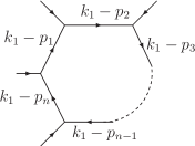
Figure 1: The generic $n$-point one-loop graph.

As was shown in ref. [19] the functional relations for these integrals can be derived from the following algebraic relation between the products of propagators

$$\prod_{r=1}^{n}\frac{1}{D_{r}}=\frac{1}{D_{0}}\sum_{r=1}^{n}x_{r}{\prod_{\begin{subarray}{c}j=1\\ j\neq r\end{subarray}}^{n}}\frac{1}{D_{j}}.$$ (2.3)

We assume that $k_{1}$ is an arbitrary momentum and $p_{j}$ correspond to external momenta. The proceeding equation is satisfied if $p_{0}$, $m_{0}^{2}$ and $x_{j}$, ($j=1,...n$) are chosen to satisfy the system of equations. In order to obtain such a system we proceed as follows. We multiply both sides of the Eq. (2.3) by the product $\prod_{j=0}^{n}D_{j}$ and get

$$D_{0}=\sum_{r=1}^{n}x_{r}D_{r},$$ (2.4)

or

$$k_{1}^{2}-2k_{1}p_{0}+p_{0}^{2}-m_{0}^{2}=\sum_{r=1}^{n}x_{r}(k_{1}^{2}-2k_{1}p_{r}+p_{r}^{2}-m_{r}^{2}).$$ (2.5)

It is assumed that $k_{1}$ will be an integration momentum and $p_{j}$, $x_{r}$ do not depend on it. Differentiating both sides of Eq.(2.5) with respect to $k_{1\mu}$, one gets a linear equation in $k_{1}$ from which two equations follow

$$1=\sum_{r=1}^{n}x_{r},$$ (2.6)

$$p_{0}=\sum_{j=1}^{n}x_{j}p_{j}.$$ (2.7)

Substituting Eqs. (2.6),(2.7) into Eq. (2.5) yields the following equation

$$m_{0}^{2}-\sum_{k=1}^{n}x_{k}m_{k}^{2}+\sum_{j=2}^{n}\sum_{l=1}^{j-1}x_{j}x_{l}s_{lj}=0,$$ (2.8)

where kinematic invariants $s_{ij}$ are defined as

$$s_{ij}=s_{i,j}=(p_{i}-p_{j})^{2}.$$ (2.9)

Solving Eq. (2.6) for one of the parameters $x_{j}$ and then substituting this solution into Eq. (2.8) gives a quadratic equation for the remaining parameters $x_{i}$. This quadratic equation can be solved with respect to one of the parameters $x_{j}$. Thus, the solution of the system of equations (2.6), (2.8) depends on $(n-2)$ of the remaining arbitrary parameters $x_{i}$ and one arbitrary mass $m_{0}$.

Integrating algebraic relation (2.3) over momentum $k_{1}$ yields functional equation for a general one-loop $n$-point integral

$$I_{n}^{(d)}(\{m_{r}^{2}\};\{s_{ik}\})=\sum_{j=1}^{n}x_{j}\left.I_{n}^{(d)}(\{m_{r}^{2}\};\{s_{ik}\})\right|_{m_{j}^{2}\rightarrow m_{0}^{2},s_{jk}\rightarrow s_{0k}}.$$ (2.10)

This equation will be our starting equation for deriving relations for the functional reduction of integrals $I_{n}^{(d)}(\{m_{r}^{2}\};\{s_{ik}\})$. In the next sections, we will consider in detail the derivation of functional relations for reducing integrals $I_{2}^{(d)}$,…,$I_{6}^{(d)}$.

3 Method of functional reduction

By choosing arbitrary parameters $x_{j}$, $m_{0}^{2}$, we can try to express the integral of interest in terms of integrals with fewer variables. If we manage to find such parameters we will actually solve the functional equation for the integral.

A systematic method for solving functional equations for Feynman integrals was presented in ref. [20]. In a sense, this is a generalization of the method that is used to solve the usual Sincov’s functional equation [21], [22], [23]

$$f(x,y)=f(x,z)-f(y,z).$$ (3.11)

By setting $z=0$ in this equation, we get a general solution

$$f(x,y)=g(x)-g(y),$$ (3.12)

where

$$g(x)=f(x,0).$$ (3.13)

I.e. the function $f(x,y)$ is a combination of its ’boundary values’, which may be completely arbitrary.

As for solving functional equations for Feynman integrals, the situation is much more complicated here - too many variables are involved, too many functions . For this reason, we used a computer to systematically search for possible relationships between the arguments of integrals leading to a decrease in the number of variables of these integrals. To reduce the number of variables, we impose the following simple conditions on the new variables $s_{j0}$, $m_{0}^{2}$

$$s_{0j}=0,~{}~{}s_{0j}-s_{0i}=0,~{}~{}s_{0j}\pm s_{ik}=0,~{}~{}s_{0j}\pm m_{0}^{2}=0,~{}~{}m_{j}^{2}\pm m_{0}^{2}=0,$$

$$m_{0}^{2}=0,~{}~{}~{}~{}s_{0j}\pm m_{0}^{2}\pm m_{k}^{2}=0,~{}~{}~{}~{}~{}(i,j,k=1{\ldots}n).~{}~{}~{}~{}~{}~{}~{}~{}~{}~{}~{}~{}~{}~{}~{}$$ (3.14)

From the set of equations obtained by combining Eqs. (3.14), (2.6) and (2.8), we have formed various systems of equations with $2,3,4,$ etc. equations in each system. Solutions of these systems of equations and analysis of these solutions were performed using computer algebra system MAPLE. The number of these systems depends on $n$ and varied from $10^{3}$ to $10^{6}$. CPU execution time ranged from a few minutes to several hours. Many solutions of these equations have been found. Some of them lead to a simultaneous decrease in the number of variables in all integrals on the right-hand side of the functional equation (2.10). In the following sections we will describe in detail how this method works.

4 Functional reduction of the 2-point integral $I_{2}^{(d)}$

We will start by considering a simple one-loop integral depending on arbitrary masses and external momentum

$$I_{2}^{(d)}(m_{1}^{2},m_{2}^{2};~{}s_{12})=\int\frac{d^{d}k_{1}}{i\pi^{{d}/{2}}}\frac{1}{[(k_{1}-p_{1})^{2}-m_{1}^{2}][(k_{1}-p_{2})^{2}-m_{2}^{2}]}.$$ (4.15)

Setting $n=2$ in the Eq. (2.3), leads to an algebraic relation between the products of two propagators

$$\frac{1}{D_{1}D_{2}}=\frac{x_{1}}{D_{0}D_{2}}+\frac{x_{2}}{D_{1}D_{0}}.$$ (4.16)

At $n=2$, according to (2.6)–(2.8), parameters $x_{j}$, $m_{0}^{2}$ and momentum $p_{0}$ in this equation must obey the following conditions

$$x_{1}+x_{2}=1,~{}~{}~{}~{}~{}~{}p_{0}=x_{1}p_{1}+x_{2}p_{2},$$

$$m_{0}^{2}-x_{1}m_{1}^{2}-x_{2}m_{2}^{2}+x_{1}x_{2}s_{12}=0.$$ (4.17)

Integrating algebraic relation (4.16) over momentum $k_{1}$ yields

$$I_{2}^{(d)}(m_{1}^{2},m_{2}^{2};s_{12})={x_{1}}I_{2}^{(d)}(m_{2}^{2},m_{0}^{2};s_{20})+{x_{2}}I_{2}^{(d)}(m_{1}^{2},m_{0}^{2};{s_{10}}).$$ (4.18)

By solving system of equations (4.17) for $x_{1}$, $x_{2}$, we get

$$x_{1}=\frac{m_{2}^{2}-m_{1}^{2}+s_{12}}{2s_{12}}\pm\frac{\sqrt{4s_{12}(m_{0}^{2}-r_{12})}}{2s_{12}},~{}~{}~{}~{}~{}~{}~{}{x_{2}}=1-x_{1}.$$ (4.19)

Both kinematic invariants $s_{10}$, $s_{20}$ can be expressed in terms of $x_{1}$ as

$$s_{10}=(p_{1}-p_{0})^{2}=(1-x_{1})^{2}s_{12}=$$

$$~{}~{}~{}~{}~{}~{}~{}~{}~{}~{}~{}~{}~{}~{}~{}~{}~{}~{}~{}~{}~{}~{}~{}m_{1}^{2}+{m_{0}^{2}}-2r_{12}\pm\frac{m_{2}^{2}-m_{1}^{2}-s_{12}}{2s_{12}}\sqrt{4s_{12}({m_{0}^{2}}-r_{12})},$$

$${s_{20}}=(p_{2}-p_{0})^{2}=x_{1}^{2}s_{12}=$$

$$~{}~{}~{}~{}~{}~{}~{}~{}~{}~{}~{}~{}~{}~{}~{}~{}~{}~{}~{}~{}~{}~{}~{}~{}m_{2}^{2}+{m_{0}^{2}}-2r_{12}\pm\frac{m_{2}^{2}-m_{1}^{2}+s_{12}}{2s_{12}}\sqrt{4s_{12}({m_{0}^{2}}-r_{12})},~{}~{}~{}$$ (4.20)

where

$$r_{12}=-\frac{\lambda_{12}}{g_{12}}=\frac{2m_{1}^{2}m_{2}^{2}+2s_{12}m_{1}^{2}+2s_{12}m_{2}^{2}-m_{1}^{4}-m_{2}^{4}-s_{12}^{2}}{4s_{12}}.$$ (4.21)

The definitions of the determinants $\lambda_{12}$, $g_{12}$ are given in Appendix.

Equation (4.18) strongly resembles Sincov’s equation (3.11). By setting the only remaining arbitrary parameter $m_{0}^{2}$ to some special value, one can try to reduce the number of variables simultaneously for both integrals on the right side of Eq. (4.18). We will consider three different cases.

Case 1. $m_{0}^{2}=0$

The most obvious choice is to take $m_{0}^{2}=0$. Substituting this value into Eq. (4.18), we obtain

$$I_{2}^{(d)}(m_{1}^{2},m_{2}^{2};s_{12})={\overline{x}_{1}}I_{2}^{(d)}(m_{2}^{2},0;{\overline{s}_{20}})+{\overline{x}_{2}}I_{2}^{(d)}(m_{1}^{2},0;{\overline{s}_{10}}),$$ (4.22)

where

$$\overline{x}_{1,2}=\left.x_{1,2}\right|_{m_{0}^{2}=0},~{}~{}~{}~{}\overline{s}_{01}=\left.s_{01}\right|_{m_{0}^{2}=0},~{}~{}~{}~{}\overline{s}_{02}=\left.s_{02}\right|_{m_{0}^{2}=0}.$$ (4.23)

The analytic expression for the integral $I_{2}^{(d)}(m^{2},0;~{}p^{2})$ is well known (see refs. [24], [25])

$$I_{2}^{(d)}(m^{2},0;~{}p^{2})=-\Gamma\left(1-\frac{d}{2}\right)m^{d-4}\,{}_{2}F_{1}\!\!\left[\begin{array}[]{c}1,2-\frac{d}{2}\,;\\ \frac{d}{2}\,;\end{array}\frac{p^{2}}{m^{2}}\right].$$ (4.24)

Note that the $\varepsilon=(4-d)/2$ expansion of the hypergeometric function ${}_{2}F_{1}$ in Eq. (4.24) is known to all orders in $\varepsilon$ [26], [27], [28]. Using Eq. (4.22) one can easily obtain $\varepsilon$ expansion of the original integral $I_{2}^{(d)}(m_{1}^{2},m_{2}^{2};s_{12})$.

Case 2. $m_{0}^{2}=r_{12}$

The second special value of $m_{0}^{2}$, which leads to a simultaneous decrease in the number of variables in both integrals on the right side of Eq. (4.18), is $m_{0}^{2}=r_{12}$. In this case, the square roots in Eqs. (4.19),(4) vanish, and we get

$$I_{2}^{(d)}(m_{1}^{2},m_{2}^{2};s_{12})=\kappa_{12}I_{2}^{(d)}(r_{12},r_{2};r_{2}-r_{12})+{\kappa_{21}}I_{2}^{(d)}(r_{12},r_{1};r_{1}-r_{12}),$$ (4.25)

where

$$\kappa_{12}=\frac{\partial r_{12}}{\partial m_{1}^{2}},~{}~{}~{}~{}~{}\kappa_{21}=\frac{\partial r_{12}}{\partial m_{2}^{2}},~{}~{}~{}~{}~{}~{}r_{i}=m_{i}^{2}.$$ (4.26)

The analytic result for integrals $I_{2}^{(d)}(r_{12},r_{j},r_{j}-r_{12})$, ($j=1,2$) can be obtained either from a Feynman parameter representation

$$I_{2}^{(d)}(r_{12},r_{j};r_{j}-r_{12})=\Gamma\left(2-\frac{d}{2}\right)\int_{0}^{1}\!\left[r_{12}+(r_{j}-r_{12})x_{1}^{2}\right]^{\frac{d}{2}-2}dx_{1},$$ (4.27)

or by solving a dimensional recurrence relation

$$(d-1)I_{2}^{(d+2)}(r_{12},r_{j};r_{j}-r_{12})=-2r_{12}I_{2}^{(d)}(r_{12},r_{j};r_{j}-r_{12})-I_{1}^{(d)}(r_{j}).~{}~{}~{}~{}$$ (4.28)

In the latter case the result reads

$$I_{2}^{(d)}(r_{12},r_{j};r_{j}-r_{12})=\frac{-\pi^{\frac{3}{2}}r_{12}^{\frac{d}{2}-2}}{2\sin\frac{\pi d}{2}\Gamma\left(\frac{d-1}{2}\right)}\sqrt{\frac{r_{12}}{r_{12}-r_{j}}}$$

$$~{}~{}~{}~{}~{}~{}~{}~{}~{}~{}~{}~{}~{}~{}~{}~{}~{}~{}~{}~{}~{}+\frac{\pi}{2r_{12}}\frac{r_{j}^{\frac{d}{2}-1}}{\sin\frac{\pi d}{2}\Gamma\left(\frac{d}{2}\right)}\,{}_{2}F_{1}\!\!\left[\begin{array}[]{c}1,\frac{d-1}{2}\,;\\ \frac{d}{2}\,;\end{array}\frac{r_{j}}{r_{12}}\right].$$ (4.31)

It is valid for $\left|r_{j}/r_{12}\right|<1$. In order to solve the dimensional recurrence relation (4.28), we used the method described in ref. [29].

By changing variable in the integral (4.27) and comparing the result with the integral representation of a ${}_{2}F_{1}$ function (13.214), we find

$$I_{2}^{(d)}(r_{12},r_{j};r_{j}-r_{12})={r_{12}^{\frac{d}{2}-2}}{\Gamma\left(2-\frac{d}{2}\right)}\,{}_{2}F_{1}\!\!\left[\begin{array}[]{c}2-\frac{d}{2},\frac{1}{2}\,;\\ \frac{3}{2}\,;\end{array}1-\frac{r_{j}}{r_{12}}\right].$$ (4.34)

esult may also be obtained by expanding the integrand in Eq. (4.27) in powers of $z_{j}=1-r_{j}/r_{12}$, assuming $\left|z_{j}\right|<1$, and then integrating with respect to $x_{1}$ term by term. Formula (4.31) can be obtained from Eq. (4.34) by performing an analytic continuation of the hypergeometric function ${}_{2}F_{1}$.

Case 3. Combination of two equations

The third reduction of integrals can be achieved in a slightly more complicated way. First, we set $m_{0}^{2}=m_{2}^{2}$ in Eq. (4.18) and obtain

$$I_{2}(m_{1}^{2},m_{2}^{2};s_{12}) = \frac{m_{1}^{2}-m_{2}^{2}}{s_{12}}I_{2}^{(d)}\left(m_{1}^{2},m_{2}^{2};~{}\frac{(m_{1}^{2}-m_{2}^{2})^{2}}{s_{12}}\right)$$ (4.35)

$$+ \frac{s_{12}-m_{1}^{2}+m_{2}^{2}}{s_{12}}I_{2}^{(d)}\left(m_{2}^{2},m_{2}^{2};~{}\frac{(s_{12}-m_{1}^{2}+m_{2}^{2})^{2}}{s_{12}}\right).$$

Then we interchange masses $m_{1}^{2}\leftrightarrow m_{2}^{2}$ in this formula and add the result to (4.35). Due to the invariance of $I_{2}^{(d)}$ under this permutation, two terms in this sum having different signs cancel out, so we get

$$I_{2}(m_{1}^{2},m_{2}^{2};~{}s_{12}) = \frac{s_{12}+m_{1}^{2}-m_{2}^{2}}{2s_{12}}I_{2}^{(d)}\left(m_{1}^{2},m_{1}^{2};~{}\frac{(s_{12}+m_{1}^{2}-m_{2}^{2})^{2}}{s_{12}}\right)$$ (4.36)

$$+ \frac{s_{12}-m_{1}^{2}+m_{2}^{2}}{2s_{12}}I_{2}^{(d)}\left(m_{2}^{2},m_{2}^{2};~{}\frac{(s_{12}-m_{1}^{2}+m_{2}^{2})^{2}}{s_{12}}\right).$$

The same result can be derived by setting $m_{0}^{2}=m_{1}^{2}$ in Eq. (4.18) and then adding the obtained result to the result obtained by setting $m_{0}^{2}=m_{2}^{2}$ in Eq. (4.18). An analytic expression for the integral with equal masses is well known (see refs. [24], [25]):

$$I_{2}^{(d)}(m^{2},m^{2};p^{2})=m^{d-4}~{}\Gamma\left(2-\frac{d}{2}\right)\,{}_{2}F_{1}\!\!\left[\begin{array}[]{c}1,2-\frac{d}{2}\,;\\ \frac{3}{2}\,;\end{array}\frac{p^{2}}{4m^{2}}\right].$$ (4.37)

Thus, we have presented three different possibilities of reducing the integral $I_{2}^{(d)}$ to a sum of integrals with fewer variables. Different reduction formulae can be used in different kinematic domains.

Using Eqs. (4.22), (4.25), (4.36) one can easily find relations between integrals that appeared in the right-hand sides of these equations. For example, setting $m_{1}^{2}=r_{12}$, $m_{2}^{2}=r_{j}$, $s_{12}=r_{j}-r_{12}$ in Eq. (4.36), we get

$$I_{2}(r_{12},r_{j};r_{j}-r_{12})=I_{2}(r_{j},r_{j};4(r_{j}-r_{12}))~{}~{}~{}~{}~{}(j=1,2).$$ (4.38)

We conclude this section with a remark about the differences between integrals found in the three reduction procedures. In Eq. (4.22), the arguments of integrals on the right side depend on square roots of ratios of polynomials, while in Eqs. (4.25), (4.36) arguments of integrals on the right side are just ratios of polynomials. In all these cases, integrals were expressed in terms of the hypergeometric function ${}_{2}F_{1}$. However, $\varepsilon=(4-d)/2$ expansion of the functions in Eq. (4.22) technically slightly simpler than expansion of the ${}_{2}F_{1}$ functions in Eqs. (4.25), (4.36). The reason is that in the first case, parameters of the ${}_{2}F_{1}$ functions are integers plus terms proportional to the $\varepsilon$ while in the ${}_{2}F_{1}$ functions from Eqs. (4.25), (4.36) some parameters are half integers. The $\varepsilon$ expansion of the ${}_{2}F_{1}$ functions with half integer parameters contains logarithms and polylogarithms depending on the square roots of the argument of the ${}_{2}F_{1}$ function [26], [27], [28], while expansion of ${}_{2}F_{1}$ functions with integer parameters do not have such square roots.

Our preliminary study shows that a similar situation takes place with integrals $I_{3}^{(d)}$ and $I_{4}^{(d)}$. Analytical results for these integrals involve the function ${}_{2}F_{1}$ as well as more complicated hypergeometric functions. We expect that finding relationships between those functions with integer and half integer parameters will be helpful in performing the $\varepsilon$ expansion of integrals $I_{3}^{(d)}$ and $I_{4}^{(d)}$.

5 Functional reduction of the 3-point integral $I_{3}^{(d)}$

Now we turn to a 3-point integral with arbitrary internal mass scales and arbitrary external momenta

$$I_{3}^{(d)}(m_{1}^{2},m_{2}^{2},m_{3}^{2};s_{23},s_{13},s_{12})=\frac{1}{i\pi^{d/2}}\int\frac{d^{d}k_{1}}{D_{1}D_{2}D_{3}}.$$ (5.39)

Setting $n=3$ in equation (2.3) leads to an algebraic relation for the products of three propagators [19]:

$$\frac{1}{D_{1}D_{2}D_{3}}=\frac{x_{\scriptscriptstyle 1}}{D_{0}D_{2}D_{3}}+\frac{x_{2}}{D_{1}D_{0}D_{3}}+\frac{x_{3}}{D_{1}D_{2}D_{0}}.$$ (5.40)

Equation (5.40) holds if

$$p_{0}=x_{1}p_{1}+x_{2}p_{2}+x_{3}p_{3},$$ (5.41)

and the parameters $m_{0}^{2}$, $x_{j}$ obey the following system of equations:

$$x_{1}+x_{2}+x_{3}=1,$$

$$x_{1}x_{2}s_{12}+x_{1}x_{\scriptscriptstyle 3}s_{13}+x_{2}x_{3}s_{23}-x_{1}m_{1}^{2}-x_{2}m_{2}^{2}-x_{3}m_{3}^{2}+m_{0}^{2}=0.$$ (5.42)

Integrating (5.40) over momentum $k_{1}$ gives a functional relation for the one-loop integral $I_{3}^{(d)}$ with arbitrary masses and kinematic variables:

$$I_{3}^{(d)}(m_{1}^{2},m_{2}^{2},m_{3}^{2};s_{23},s_{13},s_{12})$$

$$~{}~{}~{}~{}~{}~{}~{}~{}=x_{1}I_{3}^{(d)}(m^{2}_{0},m_{2}^{2},m_{3}^{2};s_{23},s_{03},s_{02})$$

$$~{}~{}~{}~{}~{}~{}~{}~{}+x_{2}I_{3}^{(d)}(m_{1}^{2},m_{0}^{2},m_{3}^{2};{s}_{03},{s}_{13},s_{01})$$

$$~{}~{}~{}~{}~{}~{}~{}~{}+x_{3}I_{3}^{(d)}(m_{1}^{2},m_{2}^{2},m_{0}^{2};s_{02},{s}_{01},{s}_{12}),$$ (5.43)

Now our aim is to find the values of $m_{0}^{2}$, $x_{j}$ ($j=1,2,3$), leading to a simultaneous reduction in the number of variables in all integrals on the right side of Eq. (5.43). Equation (5.43) will be our starting point at all steps of the functional reduction.

5.1 Functional reduction procedure

Functional reduction of the 3-point integral is not so straightforward as compared to the integral $I_{2}^{(d)}$. We will work out two-step procedure of functional reduction allowing to express an integral $I_{3}^{(d)}$ that depends on 6 variables in terms of integrals depending on 3 variables.

Reduction of the integral $I_{3}^{(d)}$, step 1

One of the solutions of the systems of equations (3.14), taken at $n=3$ and combined with equations (5.41), (5.42), leads to the desired relation

$$I_{3}\left(m_{1}^{2},m_{2}^{2},m_{3}^{2};s_{23},s_{13},s_{12}\right)$$

$$~{}~{}~{}~{}~{}~{}~{}~{}=\kappa_{123}I_{3}\left(r_{123},r_{2},r_{3};s_{23},r_{3}-r_{123},r_{2}-r_{123}\right)$$

$$~{}~{}~{}~{}~{}~{}~{}~{}+\kappa_{213}I_{3}\left(r_{123},r_{1},r_{3};s_{13},r_{3}-r_{123},r_{1}-r_{123}\right)$$

$$~{}~{}~{}~{}~{}~{}~{}~{}+\kappa_{312}I_{3}\left(r_{123},r_{2},r_{1};s_{12},r_{1}-r_{123},r_{2}-r_{123}\right),$$ (5.44)

where

$$r_{123}=-\frac{\lambda_{123}}{g_{123}},~{}~{}~{}~{}r_{i}=m_{i}^{2},$$

$$\kappa_{123}=\frac{\partial r_{123}}{\partial m_{1}^{2}},~{}~{}~{}\kappa_{213}=\frac{\partial r_{123}}{\partial m_{2}^{2}},~{}~{}~{}\kappa_{312}=\frac{\partial r_{123}}{\partial m_{3}^{2}},$$ (5.45)

and the determinants $\lambda_{123}$, $g_{123}$ are defined in Appendix. Note that all integrals on the right side of equation (5.44) depend only on 4 variables.

This is not the only functional relation that reduces the number of variables of the integral $I_{3}^{(d)}$. We have discovered another functional relationship that reduces the number of variables by one

$$I_{3}\left(m_{1}^{2},m_{2}^{2},m_{3}^{2};s_{23},s_{13},s_{12}\right)$$

$$~{}~{}~{}~{}~{}~{}~{}=\frac{s_{23}(s_{23}-s_{12}-s_{13})}{g_{123}}I_{3}\left(m_{0}^{2},m_{2}^{2},m_{3}^{2};s_{23},s_{123},s_{123}\right)$$

$$~{}~{}~{}~{}~{}~{}~{}+\frac{s_{13}(s_{13}-s_{12}-s_{23})}{g_{123}}I_{3}\left(m_{1}^{2},m_{0}^{2},m_{3}^{2};s_{123},s_{13},s_{123}\right)$$

$$~{}~{}~{}~{}~{}~{}~{}+\frac{s_{12}(s_{12}-s_{13}-s_{23})}{g_{123}}I_{3}\left(m_{1}^{2},m_{2}^{2},m_{0}^{2};s_{123},s_{123},s_{12}\right),$$ (5.46)

where

$$m_{0}^{2}=-\frac{2\delta_{3}}{g_{123}},~{}~{}~{}~{}~{}~{}s_{123}=-\frac{2s_{12}s_{13}s_{23}}{g_{123}},$$ (5.47)

$$\delta_{3}=-s_{12}s_{13}s_{23}+s_{23}(s_{12}+s_{13}-s_{23})m_{1}^{2}$$

$$~{}~{}~{}~{}~{}~{}~{}~{}~{}~{}~{}~{}~{}~{}~{}~{}~{}~{}~{}~{}~{}+s_{13}(s_{12}-s_{13}+s_{23})m_{2}^{2}-s_{12}(s_{12}-s_{13}-s_{23})m_{3}^{2},~{}~{}~{}~{}~{}$$ (5.48)

and $g_{123}$ is defined in Appendix. We have found many other functional relations that reduce the number of variables, although not in all integrals at once. However, as was shown in section 2, integrals without reducing the number of variables can be eliminated by combining various functional relations (see Eq. (4.36)). Derivation of this kind of functional relations will be studied in more detail in a forthcoming publications.

Reduction of the integral $I_{3}^{(d)}$, step 2

Now we proceed to the next step of the functional reduction. Applying relation (5.43) to the first integral on the right side of Eq. (5.44) and solving for the new variables $m_{0}^{2}$, $s_{0j}$, $x_{k}$ the corresponding system of equations from (3.14), combined with Eqs. (5.41), (5.42), leads to an equation

$$I^{(d)}_{3}\left(r_{123},r_{2},r_{3};s_{23},r_{3}-r_{123},r_{2}-r_{123}\right)$$

$$~{}~{}~{}~{}~{}~{}~{}~{}~{}~{}=\kappa_{23}I^{(d)}_{3}(r_{123},r_{23},r_{3};r_{3}-r_{23},r_{3}-r_{123},r_{23}-r_{123})$$

$$~{}~{}~{}~{}~{}~{}~{}~{}~{}~{}+\kappa_{32}I^{(d)}_{3}(r_{123},r_{23},r_{2};r_{2}-r_{23},r_{2}-r_{123},r_{23}-r_{123}).$$ (5.49)

By appropriate change of variables, two more equations for reducing other integrals in the right-hand side of Eq. (5.44), can be obtained from Eq. (5.1).

Combining Eq. (5.44), Eq. (5.1) and two equations that follow from Eq. (5.1) by changing variables, we get the final reduction formula for the integral $I_{3}^{(d)}$:

$$I_{3}^{(d)}(m_{1}^{2},m_{2}^{2},m_{3}^{2};s_{23},s_{13},s_{12})$$

$$~{}~{}~{}~{}~{}~{}~{}~{}~{}~{}~{}~{}~{}~{}=\kappa_{123}\kappa_{23}I_{3}^{(d)}(r_{123},r_{23},r_{3};r_{3}-r_{23},r_{3}-r_{123},r_{23}-r_{123})$$

$$~{}~{}~{}~{}~{}~{}~{}~{}~{}~{}~{}~{}~{}~{}+\kappa_{123}\kappa_{32}I_{3}^{(d)}(r_{123},r_{23},r_{2};r_{2}-r_{23},r_{2}-r_{123},r_{23}-r_{123})$$

$$~{}~{}~{}~{}~{}~{}~{}~{}~{}~{}~{}~{}~{}~{}+\kappa_{213}\kappa_{31}I_{3}^{(d)}(r_{123},r_{13},r_{1};r_{1}-r_{13},r_{1}-r_{123},r_{13}-r_{123})$$

$$~{}~{}~{}~{}~{}~{}~{}~{}~{}~{}~{}~{}~{}~{}+\kappa_{213}\kappa_{13}I_{3}^{(d)}(r_{123},r_{13},r_{3};r_{3}-r_{13},r_{3}-r_{123},r_{13}-r_{123})$$

$$~{}~{}~{}~{}~{}~{}~{}~{}~{}~{}~{}~{}~{}~{}+\kappa_{312}\kappa_{12}I_{3}^{(d)}(r_{123},r_{12},r_{2};r_{2}-r_{12},r_{2}-r_{123},r_{12}-r_{123})$$

$$~{}~{}~{}~{}~{}~{}~{}~{}~{}~{}~{}~{}~{}~{}+\kappa_{312}\kappa_{21}I_{3}^{(d)}(r_{123},r_{12},r_{1};r_{1}-r_{12},r_{1}-r_{123},r_{12}-r_{123}).~{}~{}~{}~{}$$ (5.50)

This formula allows one to express the integral $I_{3}^{(d)}$, which depends on 6 variables in terms of integrals depending only on 3 variables.

It is interesting to note that the replacement of masses and kinematic invariants on both sides of Eq. (5.1) with arguments of the first integral $I_{3}^{(d)}$ on the right side of this equation, i.e.

$$m_{1}^{2}\rightarrow r_{123},~{}~{}~{}~{}m_{2}\rightarrow r_{23},~{}~{}~{}~{}m_{3}^{2}\rightarrow r_{3},$$

$$s_{23}\rightarrow r_{3}-r_{23},~{}~{}~{}~{}s_{13}\rightarrow r_{3}-r_{123},~{}~{}~{}~{}s_{12}\rightarrow r_{23}-r_{123},$$ (5.51)

leads to the following transformations of the coefficients and arguments of integrals on the right side of Eq. (5.1)

$$r_{123}\rightarrow r_{123},~{}~{}~{}~{}\kappa_{123}\rightarrow 1,~{}~{}~{}~{}\kappa_{213}\rightarrow 0,~{}~{}~{}~{}\kappa_{312}\rightarrow 0,$$

$$r_{23}\rightarrow r_{23},~{}~{}~{}~{}r_{13}\rightarrow r_{123},~{}~{}~{}~{}r_{12}\rightarrow r_{123},$$

$$\kappa_{23},\kappa_{13},\kappa_{12}\rightarrow 1,~{}~{}~{}~{}\kappa_{32},\kappa_{31},\kappa_{21}\rightarrow 0.$$ (5.52)

As expected, in Eq. (5.50), after these substitutions only the first term remains. Change of variables (5.51) leads to a factorization of the determinants $\lambda$ and $g$

$$\lambda_{123}=8r_{123}(r_{23}-r_{3})(r_{123}-r_{23}),~{}~{}~{}~{}g_{123}=-8(r_{23}-r_{3})(r_{123}-r_{23}),$$

$$\lambda_{23}=-4r_{23}(r_{23}-r_{3}),~{}~{}~{}~{}g_{23}=-4(r_{3}-r_{23}),$$ (5.53)

and as follows from these relations, $r_{123}$, $r_{23}$ remain invariant under substitutions (5.51).

5.2 Analytic results for integrals depending on the MNV

Analytic result for the integral $I_{3}^{(d)}(r_{123},r_{23},r_{3};r_{3}-r_{23},r_{3}-r_{123},r_{23}-r_{123})$ can be obtained, for example, either by solving dimensional recurrence relation or by calculating the Feynman parameter integral.

The dimensional recurrence relation for this integral reads

$$(d-2)I_{3}^{(d+2)}(r_{123},r_{23},r_{3};r_{3}-r_{23},r_{3}-r_{123},r_{23}-r_{123})=$$

$$~{}~{}~{}~{}~{}~{}~{}~{}~{}~{}~{}~{}-2r_{123}I_{3}^{(d)}(r_{123},r_{23},r_{3};r_{3}-r_{23},r_{3}-r_{123},r_{23}-r_{123})$$

$$~{}~{}~{}~{}~{}~{}~{}~{}~{}~{}~{}~{}~{}~{}-I_{2}^{(d)}(r_{23},r_{3};r_{3}-r_{23}).$$ (5.54)

The solution of the dimensional recurrence relation (5.54) was obtained by the method described in ref. [29]. Assuming that $\left|r_{3}/r_{123}\right|<1$, $\left|r_{3}/r_{23}\right|<1$, $\left|r_{23}/r_{123}\right|<1$, we found the following result:

$$I_{3}^{(d)}(r_{123},r_{23},r_{3};r_{3}-r_{23},r_{3}-r_{123},r_{23}-r_{123})=$$

$$~{}~{}~{}\frac{1}{\sin\frac{\pi d}{2}}\left\{\frac{r_{123}^{\frac{d-6}{2}}}{\Gamma\left(\frac{d-2}{2}\right)}C_{3}(x,y)\right.$$

$$~{}~{}~{}+\frac{\pi^{\frac{3}{2}}r_{23}^{\frac{d-4}{2}}}{4r_{123}\Gamma\left(\frac{d-1}{2}\right)}\sqrt{\frac{r_{23}}{r_{23}-r_{3}}}~{}\,{}_{2}F_{1}\!\!\left[\begin{array}[]{c}1,\frac{d-2}{2}\,;\\ \frac{d-1}{2}\,;\end{array}\frac{r_{23}}{r_{123}}\right]$$ (5.57)

$$~{}~{}~{}\left.-\frac{\pi r_{3}^{\frac{d-2}{2}}}{4\Gamma\left(\frac{d}{2}\right)(r_{23}-r_{3})r_{123}}\sqrt{1-\frac{r_{3}}{r_{23}}}~{}F_{1}\left(\frac{d-2}{2},1,\frac{1}{2},\frac{d}{2};\frac{r_{3}}{r_{123}},\frac{r_{3}}{r_{23}}\right)\right\},~{}~{}~{}~{}$$ (5.58)

where

$$C_{3}(x,y)=\frac{\pi xy^{2}}{4(x^{2}-y^{2})^{\frac{1}{2}}}\ln\left(\frac{x-(x^{2}-y^{2})^{\frac{1}{2}}}{x+(x^{2}-y^{2})^{\frac{1}{2}}}\right),$$ (5.59)

and variables $x$, $y$ are defined as

$$x=\sqrt{\frac{r_{123}}{r_{123}-r_{3}}},~{}~{}~{}~{}~{}y=\sqrt{\frac{r_{123}}{r_{123}-r_{23}}}.$$ (5.60)

The function $C_{3}(x,y)$ was derived from a system of differential equations

$$x\frac{\partial C_{3}(x,y)}{\partial x}+y\frac{\partial C_{3}(x,y)}{\partial y}=2C_{3}(x,y),$$

$$(x^{2}-y^{2})x\frac{\partial C_{3}(x,y)}{\partial x}=-y^{2}C_{3}(x,y)-\frac{1}{2}\pi x^{2}y^{2}.$$ (5.61)

This system was obtained from the system of differential equations for the integral $I_{3}^{(d)}$. We would like to notice the coefficient $1/\sin(\pi d/2)$ in front of braces which is singular at $d=4$. Since the integral $I_{3}^{(4)}$ is finite, the terms in braces at $d=4$ must cancel. This fact makes it possible to easily obtain the hypergeometric Appell function $F_{1}$ at $d=4$ as a combination of logarithms

$$F_{1}\left(1,1,\frac{1}{2},2;\frac{r_{3}}{r_{123}},\frac{r_{3}}{r_{23}}\right)$$

$$~{}~{}~{}~{}~{}~{}~{}~{}~{}~{}~{}~{}~{}~{}~{}~{}~{}~{}~{}~{}=\frac{x^{2}\sqrt{1-y^{2}}}{1-x^{2}}\left[\ln\left(\frac{1+\sqrt{1-y^{2}}}{1-\sqrt{1-y^{2}}}\right)+\ln\left(\frac{x-\sqrt{x^{2}-y^{2}}}{x+\sqrt{x^{2}-y^{2}}}\right)\right],~{}~{}~{}~{}~{}~{}~{}$$ (5.62)

where $x$,$y$ are defined in (5.60). This expression has been checked numerically to a precision of at least 200 decimal digits.

Another hypergeometric representation of the integral $I_{3}^{(d)}$ was derived directly from the Feynman parameter integral

$$I_{3}^{(d)}(r_{123},r_{23},r_{3};r_{3}-r_{23},r_{3}-r_{123},r_{23}-r_{123})=$$

$$~{}-\Gamma\left(3-\frac{d}{2}\right)\int_{0}^{1}\!\int_{0}^{1}\!\!x_{1}\left[r_{123}-(r_{123}-r_{23})x_{1}^{2}-(r_{23}-r_{3})x_{1}^{2}x_{2}^{2}\right]^{\frac{d}{2}-3}\!dx_{1}dx_{2}.~{}~{}~{}~{}~{}~{}~{}$$ (5.63)

Expanding the integrand in powers of variables

$$z_{1}=\frac{r_{123}-r_{23}}{r_{123}},~{}~{}~{}z_{2}=\frac{r_{23}-r_{3}}{r_{123}},$$ (5.64)

assuming that $|z_{1}|<1$, $|z_{2}|<1$ and integrating over $x_{1}$, $x_{2}$, we then get

$$I_{3}^{(d)}(r_{123},r_{23},r_{3};r_{3}-r_{23},r_{3}-r_{123},r_{23}-r_{123})$$

$$~{}~{}~{}~{}~{}~{}~{}~{}~{}~{}~{}~{}~{}~{}=-\frac{1}{2}\Gamma\left({3-\frac{d}{2}}\right)\sum_{n_{1},n_{2}=0}^{\infty}\left(3-\frac{d}{2}\right)_{n_{1}+n_{2}}\frac{(1)_{n_{1}+n_{2}}}{(2)_{n_{1}+n_{2}}}\frac{\left(\frac{1}{2}\right)_{n_{2}}}{\left(\frac{3}{2}\right)_{n_{2}}}\frac{z_{1}^{n_{1}}}{n_{1}!}\frac{z_{2}^{n_{2}}}{n_{2}!}.~{}~{}~{}~{}~{}~{}~{}~{}~{}~{}~{}~{}~{}~{}$$ (5.65)

Here $(a)_{k}=\Gamma(a+k)/\Gamma(a)$ is the so-called Pochhammer symbol. The double series in Eq. (5.65) can be written [30] as the hypergeometric function $S_{1}$

$$I_{3}^{(d)}(r_{123},r_{23},r_{3};r_{3}-r_{23},r_{3}-r_{123},r_{23}-r_{123})$$

$$=-\frac{1}{2}\Gamma\left(3-\frac{d}{2}\right)r_{123}^{\frac{d}{2}-3}~{}S_{1}\left(3-\frac{d}{2},1,\frac{1}{2},2,\frac{3}{2},\frac{r_{23}-r_{3}}{r_{123}},1-\frac{r_{23}}{r_{123}}\right).$$ (5.66)

The definition of the hypergeometric function $S_{1}$ is given in Appendix. Using the formula for the analytic continuation of the function $S_{1}$ presented in ref. [30], the integral $I_{3}^{(d)}$ can be written in terms of hypergeometric functions ${}_{2}F_{1}$ and $F_{1}$ :

$$I_{3}^{(d)}(r_{123},r_{23},r_{3};r_{3}-r_{23},r_{3}-r_{123},r_{23}-r_{123})=\frac{\Gamma\left(2-\frac{d}{2}\right)}{2(r_{123}-r_{23})}r_{123}^{\frac{d}{2}-2}$$

$$~{}\times\Biggl{\{}\!\,{}_{2}F_{1}\!\!\left[\begin{array}[]{c}1,\frac{1}{2}\,;\\ \frac{3}{2}\,;\end{array}\frac{r_{3}-r_{23}}{r_{123}-r_{23}}\right]-\frac{r_{23}^{\frac{d}{2}-2}}{r_{123}^{\frac{d}{2}-2}}F_{1}\left(\frac{1}{2},1,2-\frac{d}{2},\frac{3}{2};\frac{r_{23}-r_{3}}{r_{23}-r_{123}},1-\frac{r_{3}}{r_{23}}\right)\!\Biggr{\}}.~{}~{}~{}~{}~{}~{}$$ (5.69)

The formula for the analytic continuation of the function $S_{1}$ is given in Appendix (see Eq. (13.211)). Note that the results in terms of the hypergeometric function $S_{1}$ for some $I_{3}^{(d)}$ integrals were presented in ref. [30].

6 Functional reduction of the 4-point integral $I_{4}^{(d)}$

Now we proceed to formulate a functional reduction procedure for the 4-point integral. For $n=4$, the algebraic relation (2.3) reads

$$\frac{1}{D_{1}D_{2}D_{3}D_{4}}=\frac{x_{1}}{D_{0}D_{2}D_{3}D_{4}}+\frac{x_{2}}{D_{1}D_{0}D_{3}D_{4}}+\frac{x_{3}}{D_{1}D_{2}D_{0}D_{4}}+\frac{x_{4}}{D_{1}D_{2}D_{3}D_{0}}.$$ (6.70)

Equation (6.70) holds if

$$p_{0}=x_{1}p_{1}+x_{2}p_{2}+x_{3}p_{3}+x_{4}p_{4},$$ (6.71)

and the parameters $m_{0}^{2}$, $x_{j}$ obey the following system of equations

$$x_{1}+x_{2}+x_{3}+x_{4}=1,$$

$$x_{1}x_{2}s_{12}+x_{1}x_{3}s_{13}+x_{1}x_{4}s_{14}+x_{2}x_{3}s_{23}+x_{2}x_{4}s_{24}+x_{3}x_{4}s_{34}$$

$$~{}~{}~{}~{}~{}~{}~{}~{}~{}~{}~{}~{}~{}~{}~{}~{}~{}~{}~{}~{}~{}~{}~{}~{}~{}~{}~{}~{}~{}~{}~{}~{}~{}-x_{1}m_{1}^{2}-x_{2}m_{2}^{2}-x_{3}m_{3}^{2}-x_{4}m_{4}^{2}+m_{0}^{2}=0.~{}~{}~{}~{}~{}~{}~{}$$ (6.72)

Integrating equation (6.70) over momentum $k_{1}$ yields

$$I_{4}^{(d)}(m_{1}^{2},m_{2}^{2},m_{3}^{2},m_{4}^{2};s_{12},s_{23},s_{34},s_{14},s_{24},s_{13})$$

$$~{}~{}~{}~{}~{}~{}~{}~{}~{}~{}~{}~{}~{}~{}~{}~{}~{}~{}~{}~{}=x_{1}I_{4}^{(d)}(m_{0}^{2},m_{2}^{2},m_{3}^{2},m_{4}^{2};s_{02},s_{23},s_{34},s_{04},s_{24},s_{03})$$

$$~{}~{}~{}~{}~{}~{}~{}~{}~{}~{}~{}~{}~{}~{}~{}~{}~{}~{}~{}~{}+x_{2}I_{4}^{(d)}(m_{1}^{2},m_{0}^{2},m_{3}^{2},m_{4}^{2};s_{01},s_{03},s_{34},s_{14},s_{04},s_{13})$$

$$~{}~{}~{}~{}~{}~{}~{}~{}~{}~{}~{}~{}~{}~{}~{}~{}~{}~{}~{}~{}+x_{3}I_{4}^{(d)}(m_{1}^{2},m_{2}^{2},m_{0}^{2},m_{4}^{2};s_{12},s_{02},s_{04},s_{14},s_{24},s_{01})$$

$$~{}~{}~{}~{}~{}~{}~{}~{}~{}~{}~{}~{}~{}~{}~{}~{}~{}~{}~{}~{}+x_{4}I_{4}^{(d)}(m_{1}^{2},m_{2}^{2},m_{3}^{2},m_{0}^{2};s_{12},s_{23},s_{03},s_{01},s_{02},s_{13}).$$ (6.73)

This will be our initial equation for deriving functional relations in all three steps of the reduction procedure.

6.1 Functional reduction procedure

In this subsection, we provide functional relations for expressing the integral $I_{4}^{(d)}$ that depends on 10 variables in terms of integrals $I_{4}^{(d)}$ depending on 4 variables.

Reduction of the integral $I_{4}^{(d)}$, step 1

Solving various systems of equations, formed from equations (6.72) combined with equations (3.14), taken at $n=4$, we obtained one solution which leads to the functional relation that reduces the number of variables by 3 in all integrals on the right side of Eq. (6.73). The functional relation corresponding to this solution reads

$$I_{4}(m_{1}^{2},m_{2}^{2},m_{3}^{2},m_{4}^{2};s_{12},s_{23},s_{34},s_{14},s_{24},s_{13})$$

$$~{}~{}=\kappa_{1234}I_{4}(r_{1234},r_{2},r_{3},r_{4};r_{2}-r_{1234},s_{23},s_{34},r_{4}-r_{1234},s_{24},r_{3}-r_{1234})$$

$$~{}~{}+\kappa_{2134}I_{4}(r_{1234},r_{1},r_{3},r_{4};r_{1}-r_{1234},s_{13},s_{34},r_{4}-r_{1234},s_{14},r_{3}-r_{1234})$$

$$~{}~{}+\kappa_{3124}I_{4}(r_{1234},r_{2},r_{1},r_{4};r_{2}-r_{1234},s_{12},s_{14},r_{4}-r_{1234},s_{24},r_{1}-r_{1234})$$

$$~{}~{}+\kappa_{4123}I_{4}(r_{1234},r_{2},r_{3},r_{1};r_{2}-r_{1234},s_{23},s_{13},r_{1}-r_{1234},s_{12},r_{3}-r_{1234}),~{}~{}~{}~{}~{}$$ (6.74)

where

$$r_{1234}=-\frac{\lambda_{1234}}{g_{1234}},~{}~{}~{}~{}~{}r_{i}=m_{i}^{2},$$

$$\kappa_{1234}=\frac{\partial r_{1234}}{\partial m_{1}^{2}},~{}~{}\kappa_{2134}=\frac{\partial r_{1234}}{\partial m_{2}^{2}},~{}~{}\kappa_{3124}=\frac{\partial r_{1234}}{\partial m_{3}^{2}},~{}~{}\kappa_{4123}=\frac{\partial r_{1234}}{\partial m_{4}^{2}}.~{}~{}~{}~{}~{}$$ (6.75)

In the next step, the integrals on the right side of equation (6.74) depending on 7 variables will be expressed in terms of integrals depending on 5 variables.

Reduction of the integral $I_{4}^{(d)}$, step 2

Applying the formula (6.73) to the first integral on the right side of Eq. (6.74) and solving systems of equations formed from equations (6.72) combined with equations (3.14) given for the kinematics of this integral, we found the following relation

$$I_{4}(r_{1234},r_{2},r_{3},r_{4};r_{2}-r_{1234},s_{23},s_{34},r_{4}-r_{1234},s_{24},r_{3}-r_{1234})$$

$$=\kappa_{234}I_{4}(r_{1234},r_{234},r_{3},r_{4};r_{234}-r_{1234},r_{3}-r_{234},s_{34},r_{4}-r_{1234},r_{4}-r_{234},r_{3}-r_{1234})$$

$$+\kappa_{324}I_{4}(r_{1234},r_{234},r_{2},r_{4};r_{234}-r_{1234},r_{2}-r_{234},s_{24},r_{4}-r_{1234},r_{4}-r_{234},r_{2}-r_{1234})$$

$$+\kappa_{423}I_{4}(r_{1234},r_{234},r_{3},r_{2};r_{234}-r_{1234},r_{3}-r_{234},s_{23},r_{2}-r_{1234},r_{2}-r_{234},r_{3}-r_{1234}),$$

(6.76)

where

$$r_{234}=-\frac{\lambda_{234}}{g_{234}},~{}~{}~{}~{}~{}~{}~{}\kappa_{234}=\frac{\partial r_{234}}{\partial m_{2}^{2}},~{}~{}~{}~{}~{}~{}~{}\kappa_{324}=\frac{\partial r_{234}}{\partial m_{3}^{2}},~{}~{}~{}~{}~{}~{}~{}\kappa_{423}=\frac{\partial r_{234}}{\partial m_{4}^{2}}.$$ (6.77)

Similar expressions for all other integrals on the right side of Eq. (6.74) can be obtained from Eq. (6.76) by changing variables and coefficients appropriately.

After reducing integrals depending on 7 variables to integrals depending on 5 variables, the next step is to reduce the latter integrals to integrals depending on 4 variables.

Reduction of the integral $I_{4}^{(d)}$, step 3

Applying our initial functional relation (6.73) to the first integral on the right side of Eq. (6.76) and solving, the systems of equations, corresponding to this case, we obtained several solutions. One of these solutions leads to a two-term functional relation

$$I_{4}(r_{1234},r_{234},r_{3},r_{4};r_{234}-r_{1234},r_{3}-r_{234},s_{34},r_{4}-r_{1234},r_{4}-r_{234},r_{3}-r_{1234})$$

$$=\kappa_{34}I_{4}(r_{1234},r_{234},r_{34},r_{4};$$

$$~{}~{}~{}~{}~{}~{}~{}~{}~{}~{}~{}~{}~{}~{}~{}~{}~{}r_{234}-r_{1234},r_{34}-r_{234},r_{4}-r_{34},r_{4}-r_{1234},r_{4}-r_{234},r_{34}-r_{1234})$$

$$+\kappa_{43}I_{4}(r_{1234},r_{234},r_{34},r_{3};$$

$$~{}~{}~{}~{}~{}~{}~{}~{}~{}~{}~{}~{}~{}~{}~{}~{}~{}r_{234}-r_{1234},r_{34}-r_{234},r_{3}-r_{34},r_{3}-r_{1234},r_{3}-r_{234},r_{34}-r_{1234}),$$

(6.78)

where

$$r_{34}=-\frac{\lambda_{34}}{g_{34}},~{}~{}~{}~{}~{}\kappa_{34}=\frac{\partial r_{34}}{\partial m_{3}^{2}},~{}~{}~{}~{}~{}\kappa_{43}=\frac{\partial r_{34}}{\partial m_{4}^{2}}.$$ (6.79)

Note that both integrals on the right side of Eq. (6.78) depend only on 4 variables. Combining Eqs. (6.74), (6.76), (6.78) and all required relations that follow from these equations by changing variables as mentioned previously, we obtain the final functional reduction formula for the integral $I_{4}^{(d)}$

$$I_{4}(m_{1}^{2},m_{2}^{2},m_{3}^{2},m_{4}^{2};s_{12},s_{23},s_{34},s_{14},s_{24},s_{13})$$

$$=\kappa_{1234}\kappa_{234}\kappa_{34}I_{4}^{(d)}(r_{1234},r_{234},r_{34},r_{4};$$

$$~{}~{}~{}~{}~{}~{}~{}~{}~{}~{}r_{234}-r_{1234},r_{34}-r_{234},r_{4}-r_{34},r_{4}-r_{1234},r_{4}-r_{234},r_{34}-r_{1234})$$

$$+\kappa_{1234}\kappa_{234}\kappa_{43}I_{4}^{(d)}(r_{1234},r_{234},r_{34},r_{3};$$

$$~{}~{}~{}~{}~{}~{}~{}~{}~{}~{}~{}r_{234}-r_{1234},r_{34}-r_{234},r_{3}-r_{34},r_{3}-r_{1234},r_{3}-r_{234},r_{34}-r_{1234})$$

$$+\kappa_{1234}\kappa_{324}\kappa_{24}I_{4}^{(d)}(r_{1234},r_{234},r_{24},r_{4};$$

$$~{}~{}~{}~{}~{}~{}~{}~{}~{}~{}~{}r_{234}-r_{1234},r_{24}-r_{234},r_{4}-r_{24},r_{4}-r_{1234},r_{4}-r_{234},r_{24}-r_{1234})$$

$$+\kappa_{1234}\kappa_{324}\kappa_{42}I_{4}^{(d)}(r_{1234},r_{234},r_{24},r_{2};$$

$$~{}~{}~{}~{}~{}~{}~{}~{}~{}~{}~{}r_{234}-r_{1234},r_{24}-r_{234},r_{2}-r_{24},r_{2}-r_{1234},r_{2}-r_{234},r_{24}-r_{1234})$$

$$+\kappa_{1234}\kappa_{423}\kappa_{23}I_{4}^{(d)}(r_{1234},r_{234},r_{23},r_{3};$$

$$~{}~{}~{}~{}~{}~{}~{}~{}~{}~{}~{}r_{234}-r_{1234},r_{23}-r_{234},r_{3}-r_{23},r_{3}-r_{1234},r_{3}-r_{234},r_{23}-r_{1234})$$

$$+\kappa_{1234}\kappa_{423}\kappa_{32}I_{4}^{(d)}(r_{1234},r_{234},r_{23},r_{2};$$

$$~{}~{}~{}~{}~{}~{}~{}~{}~{}~{}~{}r_{234}-r_{1234},r_{23}-r_{234},r_{2}-r_{23},r_{2}-r_{1234},r_{2}-r_{234},r_{23}-r_{1234})$$

$$+\kappa_{2134}\kappa_{134}\kappa_{34}I_{4}^{(d)}(r_{1234},r_{134},r_{34},r_{4};$$

$$~{}~{}~{}~{}~{}~{}~{}~{}~{}~{}~{}r_{134}-r_{1234},r_{34}-r_{134},r_{4}-r_{34},r_{4}-r_{1234},r_{4}-r_{134},r_{34}-r_{1234})$$

$$+\kappa_{2134}\kappa_{134}\kappa_{43}I_{4}^{(d)}(r_{1234},r_{134},r_{34},r_{3};$$

$$~{}~{}~{}~{}~{}~{}~{}~{}~{}~{}~{}r_{134}-r_{1234},r_{34}-r_{134},r_{3}-r_{34},r_{3}-r_{1234},r_{3}-r_{134},r_{34}-r_{1234})$$

$$+\kappa_{2134}\kappa_{314}\kappa_{14}I_{4}^{(d)}(r_{1234},r_{134},r_{14},r_{4};$$

$$~{}~{}~{}~{}~{}~{}~{}~{}~{}~{}~{}r_{134}-r_{1234},r_{14}-r_{134},r_{4}-r_{14},r_{4}-r_{1234},r_{4}-r_{134},r_{14}-r_{1234})$$

$$+\kappa_{2134}\kappa_{314}\kappa_{41}I_{4}^{(d)}(r_{1234},r_{134},r_{14},r_{1};$$

$$~{}~{}~{}~{}~{}~{}~{}~{}~{}~{}~{}r_{134}-r_{1234},r_{14}-r_{134},r_{1}-r_{14},r_{1}-r_{1234},r_{1}-r_{134},r_{14}-r_{1234})$$

$$+\kappa_{2134}\kappa_{413}\kappa_{13}I_{4}^{(d)}(r_{1234},r_{134},r_{13},r_{3};$$

$$~{}~{}~{}~{}~{}~{}~{}~{}~{}~{}~{}r_{134}-r_{1234},r_{13}-r_{134},r_{3}-r_{13},r_{3}-r_{1234},r_{3}-r_{134},r_{13}-r_{1234})$$

$$+\kappa_{2134}\kappa_{413}\kappa_{31}I_{4}^{(d)}(r_{1234},r_{134},r_{13},r_{1};$$

$$~{}~{}~{}~{}~{}~{}~{}~{}~{}~{}~{}r_{134}-r_{1234},r_{13}-r_{134},r_{1}-r_{13},r_{1}-r_{1234},r_{1}-r_{134},r_{13}-r_{1234})$$

$$+\kappa_{3124}\kappa_{124}\kappa_{24}I_{4}^{(d)}(r_{1234},r_{124},r_{24},r_{4};$$

$$~{}~{}~{}~{}~{}~{}~{}~{}~{}~{}~{}r_{124}-r_{1234},r_{24}-r_{124},r_{4}-r_{24},r_{4}-r_{1234},r_{4}-r_{124},r_{24}-r_{1234})$$

$$+\kappa_{3124}\kappa_{124}\kappa_{42}I_{4}^{(d)}(r_{1234},r_{124},r_{24},r_{2};$$

$$~{}~{}~{}~{}~{}~{}~{}~{}~{}~{}~{}r_{124}-r_{1234},r_{24}-r_{124},r_{2}-r_{24},r_{2}-r_{1234},r_{2}-r_{124},r_{24}-r_{1234})$$

$$+\kappa_{3124}\kappa_{214}\kappa_{14}I_{4}^{(d)}(r_{1234},r_{124},r_{14},r_{4};$$

$$~{}~{}~{}~{}~{}~{}~{}~{}~{}~{}~{}r_{124}-r_{1234},r_{14}-r_{124},r_{4}-r_{14},r_{4}-r_{1234},r_{4}-r_{124},r_{14}-r_{1234})$$

$$+\kappa_{3124}\kappa_{214}\kappa_{41}I_{4}^{(d)}(r_{1234},r_{124},r_{14},r_{1};$$

$$~{}~{}~{}~{}~{}~{}~{}~{}~{}~{}~{}r_{124}-r_{1234},r_{14}-r_{124},r_{1}-r_{14},r_{1}-r_{1234},r_{1}-r_{124},r_{14}-r_{1234})$$

$$+\kappa_{3124}\kappa_{412}\kappa_{12}I_{4}^{(d)}(r_{1234},r_{124},r_{12},r_{2};$$

$$~{}~{}~{}~{}~{}~{}~{}~{}~{}~{}~{}r_{124}-r_{1234},r_{12}-r_{124},r_{2}-r_{12},r_{2}-r_{1234},r_{2}-r_{124},r_{12}-r_{1234})$$

$$+\kappa_{3124}\kappa_{412}\kappa_{21}I_{4}^{(d)}(r_{1234},r_{124},r_{12},r_{1};$$

$$~{}~{}~{}~{}~{}~{}~{}~{}~{}~{}~{}r_{124}-r_{1234},r_{12}-r_{124},r_{1}-r_{12},r_{1}-r_{1234},r_{1}-r_{124},r_{12}-r_{1234})$$

$$+\kappa_{4123}\kappa_{123}\kappa_{23}I_{4}^{(d)}(r_{1234},r_{123},r_{23},r_{3};$$

$$~{}~{}~{}~{}~{}~{}~{}~{}~{}~{}~{}r_{123}-r_{1234},r_{23}-r_{123},r_{3}-r_{23},r_{3}-r_{1234},r_{3}-r_{123},r_{23}-r_{1234})$$

$$+\kappa_{4123}\kappa_{123}\kappa_{32}I_{4}^{(d)}(r_{1234},r_{123},r_{23},r_{2};$$

$$~{}~{}~{}~{}~{}~{}~{}~{}~{}~{}~{}r_{123}-r_{1234},r_{23}-r_{123},r_{2}-r_{23},r_{2}-r_{1234},r_{2}-r_{123},r_{23}-r_{1234})$$

$$+\kappa_{4123}\kappa_{213}\kappa_{13}I_{4}^{(d)}(r_{1234},r_{123},r_{13},r_{3};$$

$$~{}~{}~{}~{}~{}~{}~{}~{}~{}~{}~{}r_{123}-r_{1234},r_{13}-r_{123},r_{3}-r_{13},r_{3}-r_{1234},r_{3}-r_{123},r_{13}-r_{1234})$$

$$+\kappa_{4123}\kappa_{213}\kappa_{31}I_{4}^{(d)}(r_{1234},r_{123},r_{13},r_{1};$$

$$~{}~{}~{}~{}~{}~{}~{}~{}~{}~{}~{}r_{123}-r_{1234},r_{13}-r_{123},r_{1}-r_{13},r_{1}-r_{1234},r_{1}-r_{123},r_{13}-r_{1234})$$

$$+\kappa_{4123}\kappa_{312}\kappa_{12}I_{4}^{(d)}(r_{1234},r_{123},r_{12},r_{2};$$

$$~{}~{}~{}~{}~{}~{}~{}~{}~{}~{}~{}r_{123}-r_{1234},r_{12}-r_{123},r_{2}-r_{12},r_{2}-r_{1234},r_{2}-r_{123},r_{12}-r_{1234})$$

$$+\kappa_{4123}\kappa_{312}\kappa_{21}I_{4}^{(d)}(r_{1234},r_{123},r_{12},r_{1};$$

$$~{}~{}~{}~{}~{}~{}~{}~{}r_{123}-r_{1234},r_{12}-r_{123},r_{1}-r_{12},r_{1}-r_{1234},r_{1}-r_{123},r_{12}-r_{1234}).~{}~{}~{}$$ (6.80)

This formula allows us to express an integral $I_{4}^{(d)}$, that depends on 15 variables, as a linear combination of 24 integrals each of which depends only on 4 variables.

We conclude this subsection by noting an interesting property of this equation. By replacing the masses and kinematic invariants in Eq. (6.80) with corresponding arguments of the first integral on the right side of this equation

$$m_{1}^{2}\rightarrow r_{1234},~{}~{}~{}~{}m_{2}^{2}\rightarrow r_{234},~{}~{}~{}~{}m_{3}^{2}\rightarrow r_{34},~{}~{}~{}~{}m_{4}^{2}\rightarrow r_{4},$$

$$s_{12}\rightarrow r_{234}-r_{1234},~{}~{}~{}~{}s_{23}\rightarrow r_{34}-r_{234},~{}~{}~{}~{}s_{34}\rightarrow r_{4}-r_{34},~{}~{}~{}~{}$$

$$s_{14}\rightarrow r_{4}-r_{1234},~{}~{}~{}~{}s_{24}\rightarrow r_{4}-r_{234},~{}~{}~{}~{}s_{13}\rightarrow r_{34}-r_{1234},~{}~{}~{}~{}$$ (6.81)

we get the following transformations of the coefficients and arguments of integrals in this equation

$$r_{1234}\rightarrow r_{1234},~{}~{}~{}r_{234}\rightarrow r_{234},~{}~{}~{}r_{34}\rightarrow r_{34},~{}~{}~{}$$

$$\kappa_{1234},\kappa_{234},\kappa_{34}\rightarrow 1,~{}~{}~{}~{}\kappa_{2134},\kappa_{3124},\kappa_{4123}\rightarrow 0.$$ (6.82)

As a result of these substitutions, only the first integral remains on the right side of the equation. Note that the transformations (6.81) lead to a factorization of the determinants $\lambda$ and $g$ such as

$$\lambda_{1234}=16r_{1234}(r_{34}-r_{4})(r_{34}-r_{234})(r_{1234}-r_{234}),$$

$$g_{1234}=-16(r_{34}-r_{4})(r_{34}-r_{234})(r_{1234}-r_{234}).$$ (6.83)

Similar factorization holds for lower order determinants. We observed analogous factorization of determinants appearing in the final functional relations for integrals $I_{5}^{(d)}$ and $I_{6}^{(d)}$.

6.2 Analytic results for integrals depending on the MNV

Analytic expression for an integral

$$I_{4}^{(d)}(m^{2}_{1},m^{2}_{2},m^{2}_{3},m^{2}_{4};m^{2}_{2}-m^{2}_{1},m^{2}_{3}-m^{2}_{2},m^{2}_{4}-m^{2}_{3},m^{2}_{4}-m^{2}_{1},m^{2}_{4}-m^{2}_{2},m^{2}_{3}-m^{2}_{1}),$$ (6.84)

that depends on the MNV, can be obtained, for example, by solving dimensional recurrence relation or by evaluating the Feynman parameter integral.

The dimensional recurrence relation for this integral reads

$$(d-3)I_{4}^{(d+2)}(r_{1234},r_{234},r_{34},r_{4};$$

$$~{}~{}~{}~{}~{}~{}~{}r_{234}-r_{1234},r_{34}-r_{234},r_{4}-r_{34},r_{4}-r_{1234},r_{4}-r_{234},r_{34}-r_{1234})=$$

$$-2r_{1234}I_{4}^{(d)}(r_{1234},r_{234},r_{34},r_{4};$$

$$~{}~{}~{}~{}~{}~{}~{}r_{234}-r_{1234},r_{34}-r_{234},r_{4}-r_{34},r_{4}-r_{1234},r_{4}-r_{234},r_{34}-r_{1234})$$

$$~{}~{}~{}~{}~{}~{}~{}~{}~{}~{}~{}~{}~{}~{}-I_{3}^{(d)}(r_{234},r_{34},r_{4};r_{4}-r_{34},r_{4}-r_{234},r_{34}-r_{234}).$$ (6.85)

To solve this equation, we used for the integral $I_{3}^{(d)}$ an analytic result given in Eq. (5.58). Applying the method descibed in ref. [29], we get

$$I_{4}^{(d)}(r_{1234},r_{234},r_{34},r_{4};$$

$$~{}~{}~{}~{}~{}~{}~{}~{}~{}~{}~{}~{}~{}~{}~{}r_{234}-r_{1234},r_{34}-r_{234},r_{4}-r_{34},r_{4}-r_{1234},r_{4}-r_{234},r_{34}-r_{1234})=$$

$$\frac{1}{\sin{\frac{\pi d}{2}}}\Biggl{\{}\frac{r_{1234}^{\frac{d}{2}-4}}{\Gamma\left(\frac{d-3}{2}\right)}C_{4}(x,y,z)$$

$$~{}~{}~{}~{}+\frac{\pi r_{234}^{\frac{d}{2}-2}\arctan{\frac{(r_{34}-r_{4})^{\frac{1}{2}}}{(r_{234}-r_{34})^{\frac{1}{2}}}}}{4r_{1234}(r_{34}-r_{4})^{\frac{1}{2}}(r_{234}-r_{34})^{\frac{1}{2}}\Gamma\left(\frac{d-2}{2}\right)}\,{}_{2}F_{1}\!\!\left[\begin{array}[]{c}1,\frac{d-3}{2}\,;\\ \frac{d-2}{2}\,;\end{array}\frac{r_{234}}{r_{1234}}\right]$$ (6.88)

$$~{}~{}~{}~{}-\frac{\pi^{\frac{3}{2}}r_{34}^{\frac{d}{2}-2}}{8r_{1234}r_{234}\Gamma\left(\frac{d-1}{2}\right)}\left(\frac{r_{34}}{r_{34}-r_{4}}\right)^{\frac{1}{2}}\left(\frac{r_{234}}{r_{234}-r_{34}}\right)^{\frac{1}{2}}$$

$$~{}~{}~{}~{}~{}~{}~{}~{}~{}~{}~{}~{}~{}~{}~{}~{}~{}~{}\times F_{1}\left(\frac{d-3}{2},1,\frac{1}{2},\frac{d-1}{2};\frac{r_{34}}{r_{1234}},\frac{r_{34}}{r_{234}}\right)$$

$$~{}~{}~{}~{}+\frac{\pi r_{4}^{\frac{d}{2}-1}}{8r_{1234}(r_{34}-r_{4})(r_{234}-r_{4})\Gamma\left(\frac{d}{2}\right)}$$

$$~{}~{}~{}~{}~{}~{}~{}~{}~{}~{}~{}\times F_{S}\left(\frac{d-3}{2},1,1,1,1,\frac{1}{2},\frac{d}{2},\frac{d}{2},\frac{d}{2};\frac{r_{4}}{r_{1234}},\frac{r_{4}}{r_{4}-r_{234}},\frac{r_{4}}{r_{4}-r_{34}}\right)\Biggr{\}},$$ (6.89)

where

$$C_{4}(x,y,z)=\frac{\pi^{\frac{3}{2}}~{}xy^{2}z^{2}}{8(x^{2}-y^{2})^{\frac{1}{2}}(z^{2}-y^{2})^{\frac{1}{2}}}\ln\left[\frac{xz+y^{2}-(z^{2}-y^{2})^{\frac{1}{2}}(x^{2}-y^{2})^{\frac{1}{2}}}{xz+y^{2}+(z^{2}-y^{2})^{\frac{1}{2}}(x^{2}-y^{2})^{\frac{1}{2}}}\right],~{}~{}~{}$$ (6.90)

and the definition of the hypergeometric Lauricella-Saran function $F_{S}$ is given in Appendix (see Eq. (13.207)). Here the variables $x,y,z$ are defined as

$$x=\sqrt{\frac{r_{1234}}{r_{1234}-r_{4}}},~{}~{}~{}~{}y=\sqrt{\frac{r_{1234}}{r_{1234}-r_{34}}},~{}~{}~{}~{}z=\sqrt{\frac{r_{1234}}{r_{1234}-r_{234}}}.$$ (6.91)

The function $C_{4}(x,y,z)$ was obtained by solving the system of differential equations

$$x\frac{\partial C_{4}(x,y,z)}{\partial x}+y\frac{\partial C_{4}(x,y,z)}{\partial y}+z\frac{\partial C_{4}(x,y,z)}{\partial z}=3C_{4}(x,y,z),$$

$$\frac{\partial C_{4}(x,y,z)}{\partial x}=-\frac{y^{2}}{x(x^{2}-y^{2})}C_{4}(x,y,z)-\frac{\pi^{\frac{3}{2}}xy^{2}z^{2}}{4(x^{2}-y^{2})(x+z)}$$

$$\frac{\partial C_{4}(x,y,z)}{\partial z}=\frac{(2y^{2}-z^{2})}{z(y^{2}-z^{2})}C_{4}(x,y,z)+\frac{\pi^{\frac{3}{2}}~{}xy^{2}z^{2}}{4(y^{2}-z^{2})(x+z)}.$$ (6.92)

This system was derived from a system of differential equations for the integral $I_{4}^{(d)}$. The constant of integration that occurs in solving a system of differential equations (6.92) was determined by comparing the asymptotic behavior of Eq. (6.89) with the asymptotic behavior of the integral $I_{4}^{(d)}$ at $r_{1234}\rightarrow\infty$.

Note that in calculations of Feynman integrals, the Lauricella-Saran function $F_{S}$ was first discovered when calculating the one-loop box integral [31]. In ref. [31], it was shown that this function can be represented by a one-fold integral

$$F_{S}\left(\frac{d-3}{2},1,1;1,1,\frac{1}{2};\frac{d}{2},\frac{d}{2},\frac{d}{2};x,y,z\right)$$

$$~{}~{}~{}~{}~{}~{}~{}~{}~{}~{}~{}~{}~{}~{}~{}~{}=\frac{\Gamma\left(\frac{d}{2}\right)~{}(y-z)^{-\frac{1}{2}}}{\Gamma\left(\frac{d-3}{2}\right)\Gamma\left(\frac{3}{2}\right)}\int_{0}^{1}\frac{\arcsin\sqrt{\frac{(y-z)t}{1-tz}}(1-t)^{\frac{d-5}{2}}}{(1-x+tx)\sqrt{1-ty}}~{}dt.$$ (6.93)

We note that, similarly to the integral $I_{3}^{(d)}$, there is a factor $1/\sin(\pi d/2)$ in front of braces in Eq. (6.89) which is singular at $d=4$. Since the integral $I_{4}^{(4)}$ is finite, the terms in braces must cancel at $d=4$. This fact makes it possible to easily obtain the hypergeometric function $F_{S}$ at $d=4$ as a combination of logarithms

$$F_{S}\left(\frac{1}{2},1,1,1,1,\frac{1}{2},2,2,2;\frac{r_{4}}{r_{1234}},\frac{r_{4}}{r_{4}-r_{234}},\frac{r_{4}}{r_{4}-r_{34}}\right)$$

$$~{}~{}=\frac{(x^{2}-y^{2})^{\frac{1}{2}}(x^{2}-z^{2})}{(z^{2}-y^{2})^{\frac{1}{2}}(1-x^{2})x}\left\{\ln\left[\frac{xz+y^{2}-(z^{2}-y^{2})^{\frac{1}{2}}(x^{2}-y^{2})^{\frac{1}{2}}}{xz+y^{2}+(z^{2}-y^{2})^{\frac{1}{2}}(x^{2}-y^{2})^{\frac{1}{2}}}\right]\right.$$

$$~{}~{}\left.-\ln\left[\frac{x(y^{2}-z^{2})^{\frac{1}{2}}-z(y^{2}-x^{2})^{\frac{1}{2}}}{x(y^{2}-z^{2})^{\frac{1}{2}}+z(y^{2}-x^{2})^{\frac{1}{2}}}\right]+\ln\left[\frac{(z^{2}-y^{2})^{\frac{1}{2}}-(1-y^{2})^{\frac{1}{2}}}{(z^{2}-y^{2})^{\frac{1}{2}}+(1-y^{2})^{\frac{1}{2}}}\right]\right\},$$ (6.94)

where $x,y$ and $z$ are defined in Eq. (6.91). This expression has been checked numerically to a precision of at least 200 decimal digits. Complications in analytic calculation of a periodic function that appears in solving the recurrence relation for the one-loop box integral were discussed in ref. [32].

The integral $I_{4}^{(d)}$ depending on the MNV can be represented as a triple hypergeometric series. Such a representation can be derived from the Feynman parameter integral

$$I_{4}^{(d)}(r_{1234},r_{234},r_{34},r_{4};r_{234}-r_{1234},r_{34}-r_{234},r_{3}-r_{34},r_{4}-r_{234},r_{34}-r_{1234})$$

$$~{}~{}~{}~{}~{}~{}~{}~{}~{}~{}~{}~{}~{}~{}~{}~{}~{}~{}~{}~{}~{}~{}~{}=\Gamma\left(4-\frac{d}{2}\right)\int_{0}^{1}\int_{0}^{1}\int_{0}^{1}~{}x_{1}^{2}x_{2}~{}h_{4}^{\frac{d}{2}-4}dx_{1}dx_{2}dx_{3},$$ (6.95)

where

$$h_{4}=r_{1234}-(r_{1234}-r_{234})x_{1}^{2}-(r_{234}-r_{34})x_{1}^{2}x_{2}^{2}-(r_{34}-r_{4})x_{1}^{2}x_{2}^{2}x_{3}^{2},$$ (6.96)

Expanding the integrand of (6.95) with respect to the three variables

$$z_{1}=1-\frac{r_{234}}{r_{1234}},~{}~{}~{}~{}z_{2}=\frac{r_{234}-r_{34}}{r_{1234}},~{}~{}~{}~{}z_{3}=\frac{r_{34}-r_{4}}{r_{1234}},$$ (6.97)

assuming that $|z_{1}|<1$, $|z_{2}|<1$, $|z_{3}|<1$ and integrating over $x_{1}$, $x_{2}$, $x_{3}$ term by term, we obtain the series representation

$$I_{4}^{(d)}(r_{1234},r_{234},r_{34},r_{4};r_{234}-r_{1234},r_{34}-r_{234},r_{3}-r_{34},r_{4}-r_{234},r_{34}-r_{1234})$$

$$~{}~{}~{}~{}~{}~{}~{}=\frac{1}{6}\Gamma\left(4-\frac{d}{2}\right)r_{1234}^{\frac{d}{2}-4}\sum_{n_{1},n_{2},n_{3}=0}^{\infty}\left(4-\frac{d}{2}\right)_{n_{1}+n_{2}+n_{3}}$$

$$~{}~{}~{}~{}~{}~{}~{}~{}~{}~{}~{}~{}~{}~{}~{}~{}~{}~{}~{}~{}~{}~{}~{}~{}~{}~{}~{}~{}~{}~{}~{}~{}~{}\times\frac{\left(\frac{3}{2}\right)_{n_{1}+n_{2}+n_{3}}}{\left(\frac{5}{2}\right)_{n_{1}+n_{2}+n_{3}}}\frac{\left(1\right)_{n_{2}+n_{3}}}{\left(2\right)_{n_{2}+n_{3}}}\frac{\left(\frac{1}{2}\right)_{n_{3}}}{\left(\frac{3}{2}\right)_{n_{3}}}\frac{z_{1}^{n_{1}}z_{2}^{n_{2}}z_{3}^{n_{3}}}{n_{1}!n_{2}!n_{3}!}.$$ (6.98)

This series can be written as a Kampé de Fériet function [33]. The analytic continuation of this series can be expressed in terms of the hypergeometric function ${}_{2}F_{1}$, the Appell functions $F_{1}$, $F_{3}$ and various hypergeometric Lauricella-Saran functions. The formula (6.89) is an example of such a representation. Other examples can be found in refs. [34], [35]. The relationship between the hypergeometric Lauricella-Saran functions $F_{S}$ and $F_{N}$ is given in Appendix (see Eq. (13.208)).

7 Functional reduction of the 5-point integral $I_{5}^{(d)}$

In this section we describe the functional reduction of the 5-point integral. At $n=5$ the algebraic relation that follows from the Eq. (2.3) reads

$$\frac{1}{D_{1}D_{2}D_{3}D_{4}D_{5}}=\frac{x_{1}}{D_{0}D_{2}D_{3}D_{4}D_{5}}$$

$$~{}~{}~{}+\frac{x_{2}}{D_{1}D_{0}D_{3}D_{4}D_{5}}+\frac{x_{3}}{D_{1}D_{2}D_{0}D_{4}D_{5}}+\frac{x_{4}}{D_{1}D_{2}D_{3}D_{0}D_{5}}+\frac{x_{5}}{D_{1}D_{2}D_{3}D_{4}D_{0}}.~{}~{}~{}~{}~{}~{}~{}$$ (7.99)

Equation (7.99) is valid if

$$p_{0}=x_{1}p_{1}+x_{2}p_{2}+x_{3}p_{3}+x_{4}p_{4}+x_{5}p_{5},$$ (7.100)

and the parameters $m_{0}^{2}$, $x_{j}$ obey the following system of equations

$$x_{1}+x_{2}+x_{3}+x_{4}+x_{5}=1,$$

$$x_{1}x_{2}s_{12}+x_{1}x_{3}s_{13}+x_{1}x_{4}s_{14}+x_{1}x_{5}s_{15}+x_{2}x_{3}s_{23}+x_{2}x_{4}s_{24}$$

$$~{}~{}~{}~{}~{}~{}+x_{2}x_{5}s_{25}+x_{3}x_{4}s_{34}+x_{3}x_{5}s_{35}+x_{4}x_{5}s_{45}$$

$$~{}~{}~{}~{}~{}~{}-x_{1}m_{1}^{2}-x_{2}m_{2}^{2}-x_{3}m_{3}^{2}-x_{4}m_{4}^{2}-x_{5}m_{5}^{2}+m_{0}^{2}=0.~{}~{}~{}~{}~{}~{}~{}$$ (7.101)

Integrating equation (7.99) over $k_{1}$ yields a functional relation

$$I^{(d)}_{5}(m^{2}_{1},m^{2}_{2},m^{2}_{3},m^{2}_{4},m^{2}_{5};s_{12},s_{23},s_{34},s_{45},s_{15},s_{13},s_{14},s_{24},s_{25},s_{35})$$

$$=x_{1}I^{(d)}_{5}(m^{2}_{0},m^{2}_{2},m_{3}^{2},m_{4}^{2},m^{2}_{5};s_{02},s_{23},s_{34},s_{45},s_{05},s_{03},s_{04},s_{24},s_{25},s_{35})$$

$$+x_{2}I^{(d)}_{5}(m_{1}^{2},m^{2}_{0},m_{3}^{2},m_{4}^{2},m^{2}_{5};s_{01},s_{03},s_{34},s_{45},s_{15},s_{13},s_{14},s_{04},s_{05},s_{35})$$

$$+x_{3}I^{(d)}_{5}(m_{1}^{2},m^{2}_{2},m_{0}^{2},m_{4}^{2},m^{2}_{5};s_{12},s_{02},s_{04},s_{45},s_{15},s_{01},s_{14},s_{24},s_{25},s_{05})$$

$$+x_{4}I^{(d)}_{5}(m_{1}^{2},m^{2}_{2},m_{3}^{2},m_{0}^{2},m^{2}_{5};s_{12},s_{23},s_{03},s_{05},s_{15},s_{13},s_{01},s_{02},s_{25},s_{35})$$

$$+x_{5}I^{(d)}_{5}(m_{1}^{2},m^{2}_{2},m_{3}^{2},m_{4}^{2},m^{2}_{0};s_{12},s_{23},s_{34},s_{04},s_{01},s_{13},s_{14},s_{24},s_{02},s_{03}).$$ (7.102)

This equation will be our initial equation in deriving functional relations in all stages of the reduction procedure.

7.1 Functional reduction procedure

In this subsection, we describe four steps of the functional reduction procedure, that will allow us to represent the integral $I_{5}^{(d)}$, that depends on $15$ variables in terms of integrals depending on $5$ variables.

Reduction of the integral $I_{5}^{(d)}$, step 1

Systems of equations that were formed from a set of equations (3.14) and Eqs. (7.100), (7.101), have many solutions. One of these solutions leads to the following relation

$$I^{(d)}_{5}(m^{2}_{1},m^{2}_{2},m_{3}^{2},m_{4}^{2},m^{2}_{5};s_{12},s_{23},s_{34},s_{45},s_{15},s_{13},s_{14},s_{24},s_{25},s_{35})$$

$$=\kappa_{12345}I^{(d)}_{5}(r_{12345},r_{2},r_{3},r_{4},r_{5};$$

$$~{}~{}~{}~{}~{}~{}r_{2}-r_{12345},s_{23},s_{34},s_{45},r_{5}-r_{12345},r_{3}-r_{12345},r_{4}-r_{12345},s_{24},s_{25},s_{35})$$

$$+\kappa_{21345}I^{(d)}_{5}(r_{1},r_{12345},r_{3},r_{4},r_{5};$$

$$~{}~{}~{}~{}~{}~{}r_{1}-r_{12345},r_{3}-r_{12345},s_{34},s_{45},s_{15},s_{13},s_{14},r_{4}-r_{12345},r_{5}-r_{12345},s_{35})$$

$$+\kappa_{31245}I^{(d)}_{5}(r_{1},r_{2},r_{12345},r_{4},r_{5};$$

$$~{}~{}~{}~{}~{}~{}s_{12},r_{2}-r_{12345},r_{4}-r_{12345},s_{45},s_{15},r_{1}-r_{12345},s_{14},s_{24},s_{25},r_{5}-r_{12345})$$

$$+\kappa_{41235}I^{(d)}_{5}(r_{1},r_{2},r_{3},r_{12345},r_{5};$$

$$~{}~{}~{}~{}~{}~{}s_{12},s_{23},r_{3}-r_{12345},r_{5}-r_{12345},s_{15},s_{13},r_{1}-r_{12345},r_{2}-r_{12345},s_{25},s_{35})$$

$$+\kappa_{51234}I^{(d)}_{5}(r_{1},r_{2},r_{3},r_{4},r_{12345};$$

$$~{}~{}~{}~{}~{}~{}s_{12},s_{23},s_{34},r_{4}-r_{12345},r_{1}-r_{12345},s_{13},s_{14},s_{24},r_{2}-r_{12345},r_{3}-r_{12345}),$$

(7.103)

where

$$r_{12345}=-\frac{\lambda_{12345}}{g_{12345}},~{}~{}~{}\kappa_{12345}=\frac{\partial r_{12345}}{\partial m_{1}^{2}},~{}~{}~{}\kappa_{21345}=\frac{\partial r_{12345}}{\partial m_{2}^{2}},~{}~{}~{}r_{i}=m_{i}^{2},$$

$$\kappa_{31245}=~{}\frac{\partial r_{12345}}{\partial m_{3}^{2}},~{}~{}~{}\kappa_{41235}=\frac{\partial r_{12345}}{\partial m_{4}^{2}},~{}~{}~{}\kappa_{51234}=\frac{\partial r_{12345}}{\partial m_{5}^{2}}.$$

This equation is the first step in the functional reduction procedure, expressing an integral depending on 15 variables as a linear combination of integrals depending on 11 variables.

Reduction of the integral $I_{5}^{(d)}$, step 2

By setting the masses and kinematic variables in equation (7.102) to be equal to the arguments of the first integral in the right-hand side of the equation (7.103) and solving corresponding sets of systems of equations, we found

$$I^{(d)}_{5}(r_{12345},r_{2},r_{3},r_{4},r_{5};$$

$$~{}~{}~{}~{}~{}~{}r_{2}-r_{12345},s_{23},s_{34},s_{45},r_{5}-r_{12345},r_{3}-r_{12345},r_{4}-r_{12345},s_{24},s_{25},s_{35})$$

$$=\kappa_{2345}I^{(d)}_{5}(r_{12345},r_{2345},r_{3},r_{4},r_{5};r_{2345}-r_{12345},r_{3}-r_{2345},s_{34},$$

$$~{}~{}~{}~{}~{}~{}~{}~{}~{}~{}~{}s_{45},r_{5}-r_{12345},r_{3}-r_{12345},r_{4}-r_{12345},r_{4}-r_{2345},r_{5}-r_{2345},s_{35})$$

$$+\kappa_{3245}I^{(d)}_{5}(r_{12345},r_{2},r_{2345},r_{4},r_{5};r_{2}-r_{12345},r_{2}-r_{2345},r_{4}-r_{2345},$$

$$~{}~{}~{}~{}~{}~{}~{}~{}~{}~{}~{}s_{45},r_{5}-r_{12345},r_{2345}-r_{12345},r_{4}-r_{12345},s_{24},s_{25},r_{5}-r_{2345})$$

$$+\kappa_{4235}I^{(d)}_{5}(r_{12345},r_{2},r_{3},r_{2345},r_{5};r_{2}-r_{12345},s_{23},r_{3}-r_{2345},r_{5}-r_{2345},$$

$$~{}~{}~{}~{}~{}~{}~{}~{}~{}~{}~{}r_{5}-r_{12345},r_{3}-r_{12345},r_{2345}-r_{12345},r_{2}-r_{2345},s_{25},s_{35})$$

$$+\kappa_{5234}I^{(d)}_{5}(r_{12345},r_{2},r_{3},r_{4},r_{2345};r_{2}-r_{12345},s_{23},s_{34},r_{4}-r_{2345},$$

$$~{}~{}~{}~{}~{}~{}~{}~{}~{}~{}~{}r_{2345}-r_{12345},r_{3}-r_{12345},r_{4}-r_{12345},s_{24},r_{2}-r_{2345},r_{3}-r_{2345}),$$

(7.104)

where

$$r_{2345}=-\frac{\lambda_{2345}}{g_{2345}},$$

$$\kappa_{2345}=\frac{\partial r_{2345}}{\partial m_{2}^{2}},~{}~{}~{}\kappa_{3245}=\frac{\partial r_{2345}}{\partial m_{3}^{2}},~{}~{}~{}\kappa_{4235}=\frac{\partial r_{2345}}{\partial m_{4}^{2}},~{}~{}~{}\kappa_{5234}=\frac{\partial r_{2345}}{\partial m_{5}^{2}}.$$ (7.105)

Eq. (7.104) allows one to express the first integral on the right-hand side of equation (7.103), which depends on 11 variables, in terms of integrals depending on 8 variables. Similar equations that reduce the number of variables by 3 for other integrals in the right-hand side of equation (7.103) can be obtained by the proper change of arguments and coefficients in equation (7.104).

Reduction of the integral $I_{5}^{(d)}$, step 3

Integrals depending on 8 variables can be expressed in terms of integrals depending on 6 variables. Similar to the previous steps, we apply relation (7.102) to the first integral on the right-hand side of equation (7.104), and solving the corresponding sets of systems of equations, we get

$$I^{(d)}_{5}(r_{12345},r_{2345},r_{3},r_{4},r_{5};r_{2345}-r_{12345},r_{3}-r_{2345},$$

$$~{}~{}~{}~{}~{}~{}~{}~{}~{}~{}~{}s_{34},s_{45},r_{5}-r_{12345},r_{3}-r_{12345},r_{4}-r_{12345},r_{4}-r_{2345},r_{5}-r_{2345},s_{35})$$

$$=\kappa_{345}I^{(d)}_{5}(r_{12345},r_{2345},r_{345},r_{4},r_{5};r_{2345}-r_{12345},r_{345}-r_{2345},r_{4}-r_{345},$$

$$~{}~{}~{}~{}~{}~{}~{}~{}~{}~{}~{}s_{45},r_{5}-r_{12345},r_{345}-r_{12345},r_{4}-r_{12345},r_{4}-r_{2345},r_{5}-r_{2345},r_{5}-r_{345})$$

$$+\kappa_{435}I^{(d)}_{5}(r_{12345},r_{2345},r_{3},r_{345},r_{5};r_{2345}-r_{12345},r_{3}-r_{2345},r_{3}-r_{345},$$

$$~{}~{}~{}~{}~{}~{}~{}~{}~{}~{}~{}r_{5}-r_{345},r_{5}-r_{12345},r_{3}-r_{12345},r_{345}-r_{12345},r_{345}-r_{2345},r_{5}-r_{2345},s_{35})$$

$$+\kappa_{534}I^{(d)}_{5}(r_{12345},r_{2345},r_{3},r_{4},r_{345};r_{2345}-r_{12345},r_{3}-r_{2345},s_{34},r_{4}-r_{345},$$

$$~{}~{}~{}~{}~{}~{}~{}~{}~{}~{}~{}r_{345}-r_{12345},r_{3}-r_{12345},r_{4}-r_{12345},r_{4}-r_{2345},r_{345}-r_{2345},r_{3}-r_{345}),$$

(7.106)

where

$$r_{345}=-\frac{\lambda_{345}}{g_{345}},~{}~{}~{}\kappa_{345}=\frac{\partial r_{345}}{\partial m_{3}^{2}},~{}~{}~{}\kappa_{435}=\frac{\partial r_{345}}{\partial m_{4}^{2}},~{}~{}~{}\kappa_{534}=\frac{\partial r_{345}}{\partial m_{5}^{2}}.$$

The functional relation (7.106) reduces an integral depending on 8 variables to a linear combination of integrals depending on 6 variables. From equation (7.106) one can obtain similar equations for reducing all the other integrals in the right side of Eq. (7.104).

Reduction of the integral $I_{5}^{(d)}$, step 4

Now we proceed to derive the last set of reduction equations. To do this, we apply relation (7.102) to the first integral on the right side of (7.106), solve systems of equations consisting of equations (3.14), (7.100), (7.101) and find

$$I^{(d)}_{5}(r_{12345},r_{2345},r_{345},r_{4},r_{5};r_{2345}-r_{12345},r_{345}-r_{2345},r_{4}-r_{345},s_{45},$$

$$~{}~{}~{}~{}~{}~{}~{}~{}~{}~{}~{}r_{5}-r_{12345},r_{345}-r_{12345},r_{4}-r_{12345},r_{4}-r_{2345},r_{5}-r_{2345},r_{5}-r_{345})$$

$$=\kappa_{45}I^{(d)}_{5}(r_{12345},r_{2345},r_{345},r_{45},r_{5};r_{2345}-r_{12345},r_{345}-r_{2345},r_{45}-r_{345},r_{5}-r_{45},$$

$$~{}~{}~{}~{}~{}~{}~{}~{}~{}~{}~{}r_{5}-r_{12345},r_{345}-r_{12345},r_{45}-r_{12345},r_{45}-r_{2345},r_{5}-r_{2345},r_{5}-r_{345})$$

$$+\kappa_{54}I^{(d)}_{5}(r_{12345},r_{2345},r_{345},r_{4},r_{45};r_{2345}-r_{12345},r_{345}-r_{2345},r_{4}-r_{345},r_{4}-r_{45},$$

$$~{}~{}~{}~{}~{}~{}~{}~{}~{}~{}~{}r_{45}-r_{12345},r_{345}-r_{12345},r_{4}-r_{12345},r_{4}-r_{2345},r_{45}-r_{2345},r_{45}-r_{345}),$$

(7.107)

where

$$r_{45}=-\frac{\lambda_{45}}{g_{45}},~{}~{}~{}~{}~{}~{}\kappa_{45}=\frac{\partial r_{45}}{\partial m_{4}^{2}},~{}~{}~{}~{}~{}~{}\kappa_{54}=\frac{\partial r_{45}}{\partial m_{5}^{2}}.$$

Again, functional relations for reducing all other integrals on the right side of Eq. (7.106) can be obtained from (7.107) by the proper change of variables.

By combining equations (7.103), (7.104), (7.106), (7.107), and all required relations that follow from these equations by changing variables and coefficients as mentioned previously, we obtained a formula that will allow us to express the integral $I_{5}^{(d)}$, depending on 15 variables, as a linear combination of 120 integrals, each of which depends on only 5 variables. All resulting integrals in this combination depend on the MNV and have the form

$$I_{5}^{(d)}(m^{2}_{i},m^{2}_{j},m^{2}_{k},m^{2}_{l},m^{2}_{r};~{}m^{2}_{j}-m^{2}_{i},m^{2}_{k}-m^{2}_{j},m^{2}_{l}-m^{2}_{k},m^{2}_{r}-m^{2}_{l},m^{2}_{r}-m^{2}_{i},$$

$$~{}~{}~{}~{}~{}~{}~{}~{}~{}~{}~{}~{}~{}~{}~{}~{}~{}~{}~{}~{}~{}~{}~{}~{}~{}~{}m^{2}_{k}-m^{2}_{i},m^{2}_{l}-m^{2}_{i},m^{2}_{l}-m^{2}_{j},m^{2}_{r}-m^{2}_{j},m^{2}_{r}-m^{2}_{k}),$$ (7.108)

where $m^{2}_{i}$, $m^{2}_{j}$,$m^{2}_{k}$,$m^{2}_{l}$,$m^{2}_{r}$ are ratios of polynomials in masses and kinematic invariants. Coefficients in front of these integrals are also ratios of polynomials in masses and kinematic invariants.

The final reduction formula for the integral $I_{5}^{(d)}$ is too lengthy to present in the manuscript. Instead, we provide these formulae in electronic form in ancillary files distributed with this article.

7.2 Dimensional recurrence relation and series representation

The dimensional recurrence relation for the integral $I_{5}^{(d)}$ depending on the MNV reads

$$(d-4)I_{5}^{(d+2)}(r_{12345},r_{2345},r_{345},r_{45},r_{5};r_{2345}-r_{12345},r_{345}-r_{2345},r_{45}-r_{345},$$

$$~{}~{}~{}~{}~{}r_{5}-r_{45},r_{5}-r_{12345},r_{345}-r_{12345},r_{45}-r_{12345},r_{45}-r_{2345},r_{5}-r_{2345},r_{5}-r_{345})=$$

$$-2r_{12345}I_{5}^{(d)}(r_{12345},r_{2345},r_{345},r_{45},r_{5};r_{2345}-r_{12345},r_{345}-r_{2345},r_{45}-r_{345},$$

$$~{}~{}~{}~{}~{}r_{5}-r_{45},r_{5}-r_{12345},r_{345}-r_{12345},r_{45}-r_{12345},r_{45}-r_{2345},r_{5}-r_{2345},r_{5}-r_{345})$$

$$-I_{4}^{(d)}(r_{2345},r_{345},r_{45},r_{5};$$

$$~{}~{}~{}~{}~{}~{}~{}~{}~{}r_{345}-r_{2345},r_{45}-r_{345},r_{5}-r_{45},r_{5}-r_{2345},r_{5}-r_{345},r_{45}-r_{2345}).~{}~{}~{}~{}$$ (7.109)

Notice that the inhomogeneous part of this equation consists of only one term - the integral $I_{4}^{(d)}$ which also depends on the MNV. Solution of the dimensional recurrence relation for the integral $I_{5}^{(d)}$ is a bit cumbersome but straightforward. We will present the result and details of the derivation in a separate publication.

At $d=4$ the term with the integral $I_{5}^{(d+2)}$ in Eq. (7.109) drops out, and we get a simple relation

$$2r_{12345}I_{5}^{(4)}(r_{12345},r_{2345},r_{345},r_{45},r_{5};r_{2345}-r_{12345},r_{345}-r_{2345},r_{45}-r_{345},$$

$$~{}~{}~{}~{}~{}r_{5}-r_{45},r_{5}-r_{12345},r_{345}-r_{12345},r_{45}-r_{12345},r_{45}-r_{2345},r_{5}-r_{2345},r_{5}-r_{345})$$

$$=-I_{4}^{(4)}(r_{2345},r_{345},r_{45},r_{5};$$

$$~{}~{}~{}~{}~{}~{}~{}~{}~{}r_{345}-r_{2345},r_{45}-r_{345},r_{5}-r_{45},r_{5}-r_{2345},r_{5}-r_{345},r_{45}-r_{2345}).~{}~{}~{}~{}$$ (7.110)

Now we proceed to derive multiple series representation for the integral $I_{5}^{(d)}$ depending on the MNV. To do this, we will use the following Feynman parameter integral representation

$$I_{5}^{(d)}(r_{12345},r_{2345},r_{345},r_{45},r_{5};r_{2345}-r_{12345},r_{345}-r_{2345},r_{45}-r_{345},r_{5}-r_{45},r_{5}-r_{12345},$$

$$~{}~{}~{}~{}~{}~{}r_{345}-r_{12345},r_{45}-r_{12345},r_{45}-r_{2345},r_{5}-r_{2345},r_{5}-r_{345})=$$

$$~{}~{}~{}~{}~{}~{}~{}~{}~{}-\Gamma\left(5-\frac{d}{2}\right)\int_{0}^{1}\int_{0}^{1}\int_{0}^{1}\int_{0}^{1}x_{1}^{3}x_{2}^{2}x_{3}h_{5}^{\frac{d}{2}-5}dx_{1}dx_{2}dx_{3}dx_{4},$$ (7.111)

where

$$h_{5}=r_{12345}-(r_{12345}-r_{2345})x_{1}^{2}$$

$$~{}~{}~{}~{}~{}~{}-(r_{2345}-r_{345})x_{1}^{2}x_{2}^{2}-(r_{345}-r_{45})x_{1}^{2}x_{2}^{2}x_{3}^{2}-(r_{45}-r_{5})x_{1}^{2}x_{2}^{2}x_{3}^{2}x_{4}^{2}.~{}~{}$$ (7.112)

Multiple series representation of the integral $I_{5}^{(d)}$ can be derived in a similar manner as it was done for the integrals $I_{3}^{(d)}$, $I_{4}^{(d)}$. Expanding the integrand in Eq. (7.111) with respect to the four variables

$$z_{1}=\frac{r_{12345}-r_{2345}}{r_{12345}},~{}~{}~{}z_{2}=\frac{r_{2345}-r_{345}}{r_{12345}},~{}~{}~{}z_{3}=\frac{r_{345}-r_{45}}{r_{12345}},~{}~{}~{}z_{4}=\frac{r_{45}-r_{5}}{r_{12345}},$$ (7.113)

assuming that all $|z_{i}|<1$, and then integrating term by term over $x_{1}$,…,$x_{4}$, we get

$$I_{5}^{(d)}(r_{12345},r_{2345},r_{345},r_{45},r_{5};r_{2345}-r_{12345},r_{345}-r_{2345},r_{45}-r_{345},r_{5}-r_{45},$$

$$~{}~{}~{}~{}~{}r_{5}-r_{12345},r_{345}-r_{12345},r_{45}-r_{12345},r_{45}-r_{2345},r_{5}-r_{2345},r_{5}-r_{345})$$

$$~{}~{}~{}~{}=-\frac{1}{24}\Gamma\left({5-\frac{d}{2}}\right)\sum_{n_{1},n_{2},n_{3},n_{4}=0}^{\infty}\left(5-\frac{d}{2}\right)_{n_{1}+n_{2}+n_{3}+n_{4}}$$

$$~{}~{}~{}~{}~{}~{}~{}~{}~{}~{}~{}~{}~{}\times\frac{(2)_{n_{1}+n_{2}+n_{3}+n_{4}}}{(3)_{n_{1}+n_{2}+n_{3}+n_{4}}}\frac{\left(\frac{3}{2}\right)_{n_{2}+n_{3}+n_{4}}}{\left(\frac{5}{2}\right)_{n_{2}+n_{3}+n_{4}}}\frac{(1)_{n_{3}+n_{4}}}{(2)_{n_{3}+n_{4}}}\frac{\left(\frac{1}{2}\right)_{n_{4}}}{\left(\frac{3}{2}\right)_{n_{4}}}\frac{z_{1}^{n_{1}}}{n_{1}!}\frac{z_{2}^{n_{2}}}{n_{2}!}\frac{z_{3}^{n_{3}}}{n_{3}!}\frac{z_{4}^{n_{4}}}{n_{4}!}.$$ (7.114)

Note the similarity of the summand of this series to summands of the series given in Eqs. (5.65), (6.98).

8 Functional reduction of the 6-point integral $I_{6}^{(d)}$

Now we proceed to derive functional relations for reducing the 6-point integral. At $n=6$ the algebraic relation (2.3) reads

$$\frac{1}{D_{1}D_{2}D_{3}D_{4}D_{5}D_{6}}=\frac{x_{1}}{D_{0}D_{2}D_{3}D_{4}D_{5}D_{6}}+\frac{x_{2}}{D_{1}D_{0}D_{3}D_{4}D_{5}D_{6}}+\frac{x_{3}}{D_{1}D_{2}D_{0}D_{4}D_{5}D_{6}}$$

$$~{}~{}~{}+\frac{x_{4}}{D_{1}D_{2}D_{3}D_{0}D_{5}D_{6}}+\frac{x_{5}}{D_{1}D_{2}D_{3}D_{4}D_{0}D_{6}}+\frac{x_{6}}{D_{1}D_{2}D_{3}D_{4}D_{5}D_{0}}.$$ (8.115)

Equation (8.115) is valid if

$$p_{0}=x_{1}p_{1}+x_{2}p_{2}+x_{3}p_{3}+x_{4}p_{4}+x_{5}p_{5}+x_{6}p_{6},$$ (8.116)

and the parameters $m_{0}^{2}$, $x_{j}$ obey the following system of equations

$$x_{1}+x_{2}+x_{3}+x_{4}+x_{5}+x_{6}=1,$$

$$x_{1}x_{2}s_{12}+x_{1}x_{3}s_{13}+x_{1}x_{4}s_{14}+x_{1}x_{5}s_{15}+x_{1}x_{6}s_{16}+x_{2}x_{3}s_{23}+x_{2}x_{4}s_{24}$$

$$~{}~{}+x_{2}x_{5}s_{25}+x_{2}x_{6}s_{26}+x_{3}x_{4}s_{34}+x_{3}x_{5}s_{35}+x_{3}x_{6}s_{36}+x_{4}x_{5}s_{45}+x_{4}x_{6}s_{46}$$

$$~{}~{}+x_{5}x_{6}s_{56}-x_{1}m_{1}^{2}-x_{2}m_{2}^{2}-x_{3}m_{3}^{2}-x_{4}m_{4}^{2}-x_{5}m_{5}^{2}-x_{6}m_{6}^{2}+m_{0}^{2}=0.~{}~{}~{}~{}~{}~{}~{}$$ (8.117)

Integrating both sides of Eq. (8.115) over $k_{1}$ yields a functional relation

$$I^{(d)}_{6}(m_{1}^{2},m_{2}^{2},m_{3}^{2},m_{4}^{2},m_{5}^{2},m_{6}^{2};s_{12},s_{23},s_{34},s_{45},s_{56},s_{16},$$

$$~{}~{}~{}~{}~{}~{}~{}~{}~{}~{}~{}~{}~{}~{}~{}~{}~{}~{}~{}~{}~{}~{}~{}~{}~{}~{}~{}~{}~{}~{}~{}~{}~{}~{}~{}~{}~{}s_{13},s_{14},s_{15},s_{24},s_{25},s_{26},s_{35},s_{36},s_{46})$$

$$=x_{1}I^{(d)}_{6}(m_{0}^{2},m_{2}^{2},m_{3}^{2},m_{4}^{2},m_{5}^{2},m_{6}^{2};s_{02},s_{23},s_{34},s_{45},s_{56},s_{06},$$

$$~{}~{}~{}~{}~{}~{}~{}~{}~{}~{}~{}~{}~{}~{}~{}~{}~{}~{}~{}~{}~{}~{}~{}~{}~{}~{}~{}~{}~{}~{}~{}~{}~{}~{}~{}~{}~{}s_{03},s_{04},s_{05},s_{24},s_{25},s_{26},s_{35},s_{36},s_{46})$$

$$+x_{2}I^{(d)}_{6}(m_{1}^{2},m_{0}^{2},m_{3}^{2},m_{4}^{2},m_{5}^{2},m_{6}^{2};s_{01},s_{03},s_{34},s_{45},s_{56},s_{16},$$

$$~{}~{}~{}~{}~{}~{}~{}~{}~{}~{}~{}~{}~{}~{}~{}~{}~{}~{}~{}~{}~{}~{}~{}~{}~{}~{}~{}~{}~{}~{}~{}~{}~{}~{}~{}~{}~{}s_{13},s_{14},s_{15},s_{04},s_{05},s_{06},s_{35},s_{36},s_{46})$$

$$+x_{3}I^{(d)}_{6}(m_{1}^{2},m_{2}^{2},m_{0}^{2},m_{4}^{2},m_{5}^{2},m_{6}^{2};s_{12},s_{02},s_{04},s_{45},s_{56},s_{16},$$

$$~{}~{}~{}~{}~{}~{}~{}~{}~{}~{}~{}~{}~{}~{}~{}~{}~{}~{}~{}~{}~{}~{}~{}~{}~{}~{}~{}~{}~{}~{}~{}~{}~{}~{}~{}~{}~{}s_{01},s_{14},s_{15},s_{24},s_{25},s_{26},s_{05},s_{06},s_{46})$$

$$+x_{4}I^{(d)}_{6}(m_{1}^{2},m_{2}^{2},m_{3}^{2},m_{0}^{2},m_{5}^{2},m_{6}^{2};s_{12},s_{23},s_{03},s_{05},s_{56},s_{16},$$

$$~{}~{}~{}~{}~{}~{}~{}~{}~{}~{}~{}~{}~{}~{}~{}~{}~{}~{}~{}~{}~{}~{}~{}~{}~{}~{}~{}~{}~{}~{}~{}~{}~{}~{}~{}~{}~{}s_{13},s_{01},s_{15},s_{02},s_{25},s_{26},s_{35},s_{36},s_{06})$$

$$+x_{5}I^{(d)}_{6}(m_{1}^{2},m_{2}^{2},m_{3}^{2},m_{4}^{2},m_{0}^{2},m_{6}^{2};s_{12},s_{23},s_{34},s_{04},s_{06},s_{16},$$

$$~{}~{}~{}~{}~{}~{}~{}~{}~{}~{}~{}~{}~{}~{}~{}~{}~{}~{}~{}~{}~{}~{}~{}~{}~{}~{}~{}~{}~{}~{}~{}~{}~{}~{}~{}~{}~{}s_{13},s_{14},s_{01},s_{24},s_{02},s_{26},s_{03},s_{36},s_{46})$$

$$+x_{6}I^{(d)}_{6}(m_{1}^{2},m_{2}^{2},m_{3}^{2},m_{4}^{2},m_{5}^{2},m_{0}^{2};s_{12},s_{23},s_{34},s_{45},s_{05},s_{01},$$

$$~{}~{}~{}~{}~{}~{}~{}~{}~{}~{}~{}~{}~{}~{}~{}~{}~{}~{}~{}~{}~{}~{}~{}~{}~{}~{}~{}~{}~{}~{}~{}~{}~{}~{}~{}~{}~{}s_{13},s_{14},s_{15},s_{24},s_{25},s_{02},s_{35},s_{03},s_{04}).$$ (8.118)

This equation will be used in all steps of functional reduction of the integral $I_{6}^{(d)}$. Derivation of the reduction formulae is completely analogous to that of the integrals $I_{2}^{(d)}$,…,$I_{5}^{(d)}$.

8.1 Functional reduction procedure

In this subsection we will describe five steps of functional reduction procedure allowing us to represent the integral $I_{6}^{(d)}$ depending on $21$ variables in terms of integrals depending on $6$ variables.

Reduction of the integral $I_{6}^{(d)}$, step 1

In the first step we formed various systems of equations by combining Eqs. (3.14), taken at $n=6$, and Eqs. (8.116), (8.117) and solved these systems for $x_{j}$, $m_{0}^{2}$. Many solutions have been found. One of these solutions leads to a functional relation reducing 5 variables simultaneously for all integrals in the right-hand side of Eq. (8.118). The functional relation corresponding to this solution reads

$$I^{(d)}_{6}(m_{1}^{2},m_{2}^{2},m_{3}^{2},m_{4}^{2},m_{5}^{2},m_{6}^{2};s_{12},s_{23},s_{34},s_{45},s_{56},s_{16},$$

$$~{}~{}~{}~{}~{}~{}~{}~{}~{}~{}~{}~{}~{}~{}~{}~{}~{}~{}~{}~{}~{}~{}~{}~{}~{}~{}~{}~{}~{}s_{13},s_{14},s_{15},s_{24},s_{25},s_{26},s_{35},s_{36},s_{46})$$

$$=\kappa_{123456}I^{(d)}_{6}(r_{123456},r_{2},r_{3},r_{4},r_{5},r_{6};r_{2}-r_{123456},s_{23},s_{34},s_{45},s_{56},r_{6}-r_{123456},$$

$$~{}~{}~{}~{}~{}~{}~{}~{}~{}~{}~{}~{}r_{3}-r_{123456},r_{4}-r_{123456},r_{5}-r_{123456},s_{24},s_{25},s_{26},s_{35},s_{36},s_{46})$$

$$+\kappa_{213456}I^{(d)}_{6}(r_{1},r_{123456},r_{3},r_{4},r_{5},r_{6};r_{1}-r_{123456},r_{3}-r_{123456},s_{34},s_{45},s_{56},s_{16},$$

$$~{}~{}~{}~{}~{}~{}~{}~{}~{}~{}~{}~{}~{}s_{13},s_{14},s_{15},r_{4}-r_{123456},r_{5}-r_{123456},r_{6}-r_{123456},s_{35},s_{36},s_{46})$$

$$+\kappa_{312456}I^{(d)}_{6}(r_{1},r_{2},r_{123456},r_{4},r_{5},r_{6};s_{12},r_{2}-r_{123456},r_{4}-r_{123456},s_{45},s_{56},s_{16},$$

$$~{}~{}~{}~{}~{}~{}~{}~{}~{}~{}~{}~{}~{}~{}r_{1}-r_{123456},s_{14},s_{15},s_{24},s_{25},s_{26},r_{5}-r_{123456},r_{6}-r_{123456},s_{46})$$

$$+\kappa_{412356}I^{(d)}_{6}(r_{1},r_{2},r_{3},r_{123456},r_{5},r_{6};s_{12},s_{23},r_{3}-r_{123456},r_{5}-r_{123456},s_{56},$$

$$~{}~{}~{}~{}~{}~{}~{}~{}~{}~{}~{}~{}~{}~{}s_{16},s_{13},r_{1}-r_{123456},s_{15},r_{2}-r_{123456},s_{25},s_{26},s_{35},s_{36},r_{6}-r_{123456})$$

$$+\kappa_{512346}I^{(d)}_{6}(r_{1},r_{2},r_{3},r_{4},r_{123456},r_{6};s_{12},s_{23},s_{34},r_{4}-r_{123456},r_{6}-r_{123456},$$

$$~{}~{}~{}~{}~{}~{}~{}~{}~{}~{}~{}~{}~{}~{}s_{16},s_{13},s_{14},r_{1}-r_{123456},s_{24},r_{2}-r_{123456},s_{26},r_{3}-r_{123456},s_{36},s_{46})$$

$$+\kappa_{612345}I^{(d)}_{6}(r_{1},r_{2},r_{3},r_{4},r_{5},r_{123456};s_{12},s_{23},s_{34},s_{45},r_{5}-r_{123456},r_{1}-r_{123456},$$

$$~{}~{}~{}~{}~{}~{}~{}~{}~{}~{}~{}~{}~{}~{}s_{13},s_{14},s_{15},s_{24},s_{25},r_{2}-r_{123456},s_{35},r_{3}-r_{123456},r_{4}-r_{123456}),$$

(8.119)

where

$$r_{123456}=-\frac{\lambda_{123456}}{g_{123456}},~{}\kappa_{123456}=\frac{\partial r_{123456}}{\partial m_{1}^{2}},~{}\kappa_{213456}=\frac{\partial r_{123456}}{\partial m_{2}^{2}},~{}\kappa_{213456}=\frac{\partial r_{123456}}{\partial m_{3}^{2}},$$

$$~{}~{}~{}~{}\kappa_{213456}=\frac{\partial r_{123456}}{\partial m_{4}^{2}},~{}~{}\kappa_{213456}=\frac{\partial r_{123456}}{\partial m_{5}^{2}},~{}~{}\kappa_{612345}=\frac{\partial r_{123456}}{\partial m_{6}^{2}},~{}~{}r_{i}=m_{i}^{2}.$$ (8.120)

There are several other solutions of the systems of equations (3.14), (8.116), (8.117) allowing us to reduce the number of variables simultaneously for all integrals in the right-hand side of Eq. (8.118) but the number of variables reducible by functional relations corresponding to these solutions were less than 5. We obtained also many solutions leading to the functional relations reducing the number of variables but not for all integrals simultaneously. Some of these solutions depend on square roots of polynomials in kinematic variables and masses.

Reduction of the integral $I_{6}^{(d)}$, step 2

In the second step of the reduction we take arguments of the first integral in the right-hand side of equation (8.119) and substitute them into the initial functional equation (8.118). By solving systems of equations composed of equations (3.14) and equations (8.116), (8.117), for the new unknowns $m_{0}^{2}$, $s_{0j}$, $x_{j}$, we found a solution allowing us to reduce four variables simultaneously for all integrals. This solution leads the following reduction formula

$$I^{(d)}_{6}(r_{123456},r_{2},r_{3},r_{4},r_{5},r_{6};r_{2}-r_{123456},s_{23},s_{34},s_{45},s_{56},r_{6}-r_{123456},$$

$$~{}~{}~{}~{}~{}~{}~{}~{}~{}~{}~{}~{}r_{3}-r_{123456},r_{4}-r_{123456},r_{5}-r_{123456},s_{24},s_{25},s_{26},s_{35},s_{36},s_{46})$$

$$=\kappa_{23456}I^{(d)}_{6}(r_{123456},r_{23456},r_{3},r_{4},r_{5},r_{6};r_{23456}-r_{123456},r_{3}-r_{23456},s_{34},s_{45},s_{56},r_{6}-r_{123456},$$

$$~{}~{}~{}~{}~{}~{}~{}r_{3}-r_{123456},r_{4}-r_{123456},r_{5}-r_{123456},r_{4}-r_{23456},r_{5}-r_{23456},r_{6}-r_{23456},s_{35},s_{36},s_{46})$$

$$+\kappa_{32456}I^{(d)}_{6}(r_{123456},r_{2},r_{23456},r_{4},r_{5},r_{6};r_{2}-r_{123456},r_{2}-r_{23456},r_{4}-r_{23456},s_{45},s_{56},r_{6}-r_{123456},$$

$$~{}~{}~{}~{}~{}~{}~{}~{}~{}~{}~{}~{}r_{23456}-r_{123456},r_{4}-r_{123456},r_{5}-r_{123456},s_{24},s_{25},s_{26},r_{5}-r_{23456},r_{6}-r_{23456},s_{46})$$

$$+\kappa_{42356}I^{(d)}_{6}(r_{123456},r_{2},r_{3},r_{23456},r_{5},r_{6};r_{2}-r_{123456},s_{23},r_{3}-r_{23456},r_{5}-r_{23456},s_{56},r_{6}-r_{123456},$$

$$~{}~{}~{}~{}~{}~{}~{}~{}~{}~{}~{}~{}r_{3}-r_{123456},r_{23456}-r_{123456},r_{5}-r_{123456},r_{2}-r_{23456},s_{25},s_{26},s_{35},s_{36},r_{6}-r_{23456})$$

$$+\kappa_{52346}I^{(d)}_{6}(r_{123456},r_{2},r_{3},r_{4},r_{23456},r_{6};r_{2}-r_{123456},s_{23},s_{34},r_{4}-r_{23456},r_{6}-r_{23456},r_{6}-r_{123456},$$

$$~{}~{}~{}~{}~{}~{}~{}~{}~{}~{}~{}~{}r_{3}-r_{123456},r_{4}-r_{123456},r_{23456}-r_{123456},s_{24},r_{2}-r_{23456},s_{26},r_{3}-r_{23456},s_{36},s_{46})$$

$$+\kappa_{62345}I^{(d)}_{6}(r_{123456},r_{2},r_{3},r_{4},r_{5},r_{23456};r_{2}-r_{123456},s_{23},s_{34},s_{45},r_{5}-r_{23456},r_{23456}-r_{123456},$$

$$~{}~{}~{}~{}~{}~{}~{}~{}~{}~{}~{}~{}r_{3}-r_{123456},r_{4}-r_{123456},r_{5}-r_{123456},s_{24},s_{25},r_{2}-r_{23456},s_{35},r_{3}-r_{23456},r_{4}-r_{23456}),$$

(8.121)

where

$$r_{23456}=-\frac{\lambda_{23456}}{g_{23456}},~{}~{}~{}\kappa_{23456}=\frac{\partial r_{23456}}{\partial m_{2}^{2}},~{}~{}~{}\kappa_{32456}=\frac{\partial r_{23456}}{\partial m_{3}^{2}},$$

$$\kappa_{42356}=\frac{\partial r_{23456}}{\partial m_{4}^{2}},~{}~{}~{}\kappa_{52346}=\frac{\partial r_{23456}}{\partial m_{5}^{2}},~{}~{}~{}\kappa_{62345}=\frac{\partial r_{23456}}{\partial m_{6}^{2}}.$$ (8.122)

Similar considerations apply to other integrals from the right-hand side of the equation (8.119). Hence, with the aid of the functional relation (8.121), the original integral depending on 16 variables will be reduced to a combination of integrals depending on 12 variables.

Reduction of the integral $I_{6}^{(d)}$, step 3

In the third step, integrals depending on 12 variables were reduced to integrals depending on 9 variables. We substitute arguments of the first integral in the right side of equation (8.121) into our initial equation (8.118) and solve systems of equations composed of equations (3.14) and (8.116), (8.117) for the new unknowns $x_{j}$, $m_{0}^{2}$.

One of the obtained solutions yields the required reduction formula

$$I^{(d)}_{6}(r_{123456},r_{23456},r_{3},r_{4},r_{5},r_{6};r_{23456}-r_{123456},r_{3}-r_{23456},s_{34},s_{45},s_{56},r_{6}-r_{123456},$$

$$~{}~{}~{}~{}~{}~{}~{}r_{3}-r_{123456},r_{4}-r_{123456},r_{5}-r_{123456},r_{4}-r_{23456},r_{5}-r_{23456},r_{6}-r_{23456},s_{35},s_{36},s_{46})$$

$$=\kappa_{3456}I^{(d)}_{6}(r_{123456},r_{23456},r_{3456},r_{4},r_{5},r_{6};r_{23456}-r_{123456},r_{3456}-r_{23456},r_{4}-r_{3456},$$

$$~{}~{}~{}~{}~{}~{}~{}s_{45},s_{56},r_{6}-r_{123456},r_{3456}-r_{123456},r_{4}-r_{123456},r_{5}-r_{123456},r_{4}-r_{23456},$$

$$~{}~{}~{}~{}~{}~{}~{}~{}r_{5}-r_{23456},r_{6}-r_{23456},r_{5}-r_{3456},r_{6}-r_{3456},s_{46})$$

$$+\kappa_{4356}I^{(d)}_{6}(r_{123456},r_{23456},r_{3},r_{3456},r_{5},r_{6};r_{23456}-r_{123456},r_{3}-r_{23456},r_{3}-r_{3456},$$

$$~{}~{}~{}~{}~{}~{}~{}r_{5}-r_{3456},s_{56},r_{6}-r_{123456},r_{3}-r_{123456},r_{3456}-r_{123456},$$

$$~{}~{}~{}~{}~{}~{}~{}r_{5}-r_{123456},r_{3456}-r_{23456},r_{5}-r_{23456},r_{6}-r_{23456},s_{35},s_{36},r_{6}-r_{3456})$$

$$+\kappa_{5346}I^{(d)}_{6}(r_{123456},r_{23456},r_{3},r_{4},r_{3456},r_{6};r_{23456}-r_{123456},r_{3}-r_{23456},s_{34},$$

$$~{}~{}~{}~{}~{}~{}~{}r_{4}-r_{3456},r_{6}-r_{3456},r_{6}-r_{123456},r_{3}-r_{123456},r_{4}-r_{123456},r_{3456}-r_{123456},$$

$$~{}~{}~{}~{}~{}~{}~{}r_{4}-r_{23456},r_{3456}-r_{23456},r_{6}-r_{23456},r_{3}-r_{3456},s_{36},s_{46})$$

$$+\kappa_{6345}I^{(d)}_{6}(r_{123456},r_{23456},r_{3},r_{4},r_{5},r_{3456};r_{23456}-r_{123456},r_{3}-r_{23456},s_{34},$$

$$~{}~{}~{}~{}~{}~{}~{}s_{45},r_{5}-r_{3456},r_{3456}-r_{123456},r_{3}-r_{123456},r_{4}-r_{123456},r_{5}-r_{123456},$$

$$~{}~{}~{}~{}~{}~{}~{}r_{4}-r_{23456},r_{5}-r_{23456},r_{3456}-r_{23456},s_{35},r_{3}-r_{3456},r_{4}-r_{3456}),$$

(8.123)

where

$$r_{3456}=-\frac{\lambda_{3456}}{g_{3456}},~{}~{}~{}\kappa_{3456}=\frac{\partial r_{3456}}{\partial m_{3}^{2}},~{}~{}~{}\kappa_{4356}=\frac{\partial r_{3456}}{\partial m_{4}^{2}},$$

$$\kappa_{5346}=\frac{\partial r_{3456}}{\partial m_{5}^{2}},~{}~{}~{}\kappa_{6345}=\frac{\partial r_{3456}}{\partial m_{6}^{2}}.$$ (8.124)

Functional relations for reducing other integrals from the right-hand side of Eq. (8.121) can be obtained from Eq. (8.123) by appropriate change of variables.

Reduction of the integral $I_{6}^{(d)}$, step 4

In the next step we derive formula for expressing integrals depending on 9 variables in terms of integrals depending on 7 variables. Again, as it was done in the previous step, we substitute arguments of the first integral on the right-hand side of Eq. (8.123) into Eq. (8.118), solve appropriate systems of equations for the new unknowns and get

$$I^{(d)}_{6}(r_{123456},r_{23456},r_{3456},r_{4},r_{5},r_{6};r_{23456}-r_{123456},r_{3456}-r_{23456},r_{4}-r_{3456},$$

$$~{}~{}~{}~{}~{}~{}~{}s_{45},s_{56},r_{6}-r_{123456},r_{3456}-r_{123456},r_{4}-r_{123456},r_{5}-r_{123456},r_{4}-r_{23456},$$

$$~{}~{}~{}~{}~{}~{}~{}~{}r_{5}-r_{23456},r_{6}-r_{23456},r_{5}-r_{3456},r_{6}-r_{3456},s_{46})$$

$$~{}=\kappa_{456}I^{(d)}_{6}(r_{123456},r_{23456},r_{3456},r_{456},r_{5},r_{6};r_{23456}-r_{123456},r_{3456}-r_{23456},r_{456}-r_{3456},$$

$$~{}~{}~{}~{}~{}~{}~{}r_{5}-r_{456},s_{56},r_{6}-r_{123456},r_{3456}-r_{123456},r_{456}-r_{123456},r_{5}-r_{123456},r_{456}-r_{23456},$$

$$~{}~{}~{}~{}~{}~{}~{}~{}r_{5}-r_{23456},r_{6}-r_{23456},r_{5}-r_{3456},r_{6}-r_{3456},r_{6}-r_{456})$$

$$+\kappa_{546}I^{(d)}_{6}(r_{123456},r_{23456},r_{3456},r_{4},r_{456},r_{6};r_{23456}-r_{123456},r_{3456}-r_{23456},r_{4}-r_{3456},$$

$$~{}~{}~{}~{}~{}~{}~{}r_{4}-r_{456},r_{6}-r_{456},r_{6}-r_{123456},r_{3456}-r_{123456},r_{4}-r_{123456},r_{4}-r_{23456},$$

$$~{}~{}~{}~{}~{}~{}~{}r_{456}-r_{123456},r_{456}-r_{23456},r_{6}-r_{23456},r_{456}-r_{3456},r_{6}-r_{3456},s_{46})$$

$$+\kappa_{645}I^{(d)}_{6}(r_{123456},r_{23456},r_{3456},r_{4},r_{5},r_{456};r_{23456}-r_{123456},r_{3456}-r_{23456},r_{4}-r_{3456},$$

$$~{}~{}~{}~{}~{}~{}~{}s_{45},r_{5}-r_{456},r_{456}-r_{123456},r_{3456}-r_{123456},r_{4}-r_{123456},r_{5}-r_{123456},r_{4}-r_{23456},$$

$$~{}~{}~{}~{}~{}~{}~{}~{}r_{5}-r_{23456},r_{456}-r_{23456},r_{5}-r_{3456},r_{456}-r_{3456},r_{4}-r_{456}),$$

(8.125)

where

$$r_{456}=-\frac{\lambda_{456}}{g_{456}},~{}~{}~{}\kappa_{456}=\frac{\partial r_{456}}{\partial m_{4}^{2}},~{}~{}~{}\kappa_{546}=\frac{\partial r_{456}}{\partial m_{5}^{2}},~{}~{}~{}\kappa_{645}=\frac{\partial r_{456}}{\partial m_{6}^{2}}.$$ (8.126)

Notice that all integrals in the right-hand side of equation (8.125) depend on 7 variables. These integrals may be expressed in terms of integrals depending on 6 variables.

Reduction of the integral $I_{6}^{(d)}$, step 5

The final formula for the first integral on the right side of Eq. (8.125) was derived by the same method which was used in the previous steps and reads

$$I^{(d)}_{6}(r_{123456},r_{23456},r_{3456},r_{456},r_{5},r_{6};r_{23456}-r_{123456},r_{3456}-r_{23456},r_{456}-r_{3456},$$

$$~{}~{}~{}~{}~{}~{}~{}r_{5}-r_{456},s_{56},r_{6}-r_{123456},r_{3456}-r_{123456},r_{456}-r_{123456},r_{5}-r_{123456},r_{456}-r_{23456},$$

$$~{}~{}~{}~{}~{}~{}~{}~{}r_{5}-r_{23456},r_{6}-r_{23456},r_{5}-r_{3456},r_{6}-r_{3456},r_{6}-r_{456})$$

$$=\kappa_{56}I^{(d)}_{6}(r_{123456},r_{23456},r_{3456},r_{456},r_{56},r_{6};r_{23456}-r_{123456},r_{3456}-r_{23456},r_{456}-r_{3456},$$

$$~{}~{}~{}~{}~{}~{}~{}r_{56}-r_{456},r_{6}-r_{56},r_{6}-r_{123456},r_{3456}-r_{123456},r_{456}-r_{123456},r_{56}-r_{123456},$$

$$~{}~{}~{}~{}r_{456}-r_{23456},r_{56}-r_{23456},r_{6}-r_{23456},r_{56}-r_{3456},r_{6}-r_{3456},r_{6}-r_{456})$$

$$+\kappa_{65}I^{(d)}_{6}(r_{123456},r_{23456},r_{3456},r_{456},r_{5},r_{56};r_{23456}-r_{123456},r_{3456}-r_{23456},r_{456}-r_{3456},$$

$$~{}~{}~{}~{}~{}~{}~{}r_{5}-r_{456},r_{6}-r_{56},r_{56}-r_{123456},r_{3456}-r_{123456},r_{456}-r_{123456},r_{5}-r_{123456},$$

$$~{}~{}~{}~{}r_{456}-r_{23456},r_{5}-r_{23456},r_{56}-r_{23456},r_{5}-r_{3456},r_{56}-r_{3456},r_{56}-r_{456}),$$

(8.127)

where

$$r_{56}=-\frac{\lambda_{56}}{g_{56}},~{}~{}~{}~{}\kappa_{56}=\frac{\partial r_{56}}{\partial m_{5}^{2}},~{}~{}~{}~{}\kappa_{65}=\frac{\partial r_{56}}{\partial m_{6}^{2}}.$$ (8.128)

Analogous formulae for the reduction of other integrals on the right-hand side of Eq. (8.125) can be obtained form Eq. (8.127) by changing variables appropriately. This completes the derivation of the reduction formulae for the integral $I_{6}^{(d)}$.

Composition of equations (8.119), (8.121), (8.123), (8.125), (8.127) and all required relations that follow from these equations by changing variables as mentioned previously, gives a formula for the complete functional reduction of the integral $I_{6}^{(d)}$. This formula represent integral depending on 21 variables as a sum of 720 integrals, each of which depends only on 6 variables. All resulting integrals in this sum have the form

$$I_{6}^{(d)}(m^{2}_{i},m^{2}_{j},m^{2}_{k},m^{2}_{l},m^{2}_{r},m^{2}_{s};~{}~{}m^{2}_{j}-m^{2}_{i},m^{2}_{k}-m^{2}_{j},m^{2}_{l}-m^{2}_{k},m^{2}_{r}-m^{2}_{l},$$

$$~{}~{}~{}~{}~{}m^{2}_{s}-m^{2}_{r},m^{2}_{s}-m^{2}_{i},m^{2}_{k}-m^{2}_{i},m^{2}_{l}-m^{2}_{i},m^{2}_{r}-m^{2}_{i},m^{2}_{l}-m^{2}_{j},$$

$$~{}~{}~{}~{}~{}~{}~{}m^{2}_{r}-m^{2}_{j},m^{2}_{s}-m^{2}_{j},m^{2}_{r}-m^{2}_{k},m^{2}_{s}-m^{2}_{k},m^{2}_{s}-m^{2}_{l}),$$ (8.129)

where $m^{2}_{i}$, $m^{2}_{j}$, $m^{2}_{k}$, $m^{2}_{l}$, $m^{2}_{r}$, $m^{2}_{s}$ are ratios of polynomials in masses and kinematic invariants. Coefficients in front of these integrals are also ratios of polynomials in masses and kinematic invariants.

The final formula of the reduction is too lengthy to display here, but we provide it in a computer-readable ancillary file attached to this article.

8.2 Dimensional recurrence relation and series representation

An analytic result for the integral $I_{6}^{(d)}$ can be obtained, for example, by solving a dimensional recurrence relation or by evaluating Feynman parameter integral.

Dimensional recurrence relation for the integral $I_{6}^{(d)}$ depending on the MNV reads

$$(d-5)I^{(d+2)}_{6}(r_{123456},r_{23456},r_{3456},r_{456},r_{56},r_{6};r_{23456}-r_{123456},r_{3456}-r_{23456},r_{456}-r_{3456},$$

$$~{}~{}~{}~{}~{}~{}~{}r_{56}-r_{456},r_{6}-r_{56},r_{6}-r_{123456},r_{3456}-r_{123456},r_{456}-r_{123456},r_{56}-r_{123456},$$

$$~{}~{}~{}~{}r_{456}-r_{23456},r_{56}-r_{23456},r_{6}-r_{23456},r_{56}-r_{3456},r_{6}-r_{3456},r_{6}-r_{456})=$$

$$-2r_{123456}I^{(d)}_{6}(r_{123456},r_{23456},r_{3456},r_{456},r_{56},r_{6};r_{23456}-r_{123456},r_{3456}-r_{23456},r_{456}-r_{3456},$$

$$~{}~{}~{}~{}~{}~{}~{}r_{56}-r_{456},r_{6}-r_{56},r_{6}-r_{123456},r_{3456}-r_{123456},r_{456}-r_{123456},r_{56}-r_{123456},$$

$$~{}~{}~{}~{}r_{456}-r_{23456},r_{56}-r_{23456},r_{6}-r_{23456},r_{56}-r_{3456},r_{6}-r_{3456},r_{6}-r_{456})$$

$$-I^{(d)}_{5}(r_{23456},r_{3456},r_{456},r_{56},r_{6};r_{3456}-r_{23456},r_{456}-r_{3456},r_{56}-r_{456},r_{6}-r_{56},r_{6}-r_{23456},$$

$$~{}~{}~{}~{}~{}~{}~{}r_{456}-r_{23456},r_{56}-r_{23456},r_{56}-r_{3456},r_{6}-r_{3456},r_{6}-r_{456}).$$ (8.130)

Notice that the inhomogeneous term in this equation is an integral depending on the MNV. Solution of this recurrence relation is straightforward but cumbersome. The result is a bit lengthy and for this reason it will not be presented in this article.

We obtained the following Feynman parameter representation of this integral

$$I_{6}^{(d)}(r_{123456},r_{23456},r_{3456},r_{456},r_{56},r_{6};\{s_{ij}\})$$

$$~{}~{}~{}~{}~{}~{}~{}~{}~{}~{}~{}~{}~{}~{}~{}~{}~{}~{}~{}~{}~{}~{}~{}~{}=\Gamma\left(6-\frac{d}{2}\right)\int_{0}^{1}...\int_{0}^{1}~{}x_{1}^{4}x_{2}^{3}x_{3}^{2}x_{4}~{}h_{6}^{\frac{d}{2}-6}dx_{1}...dx_{5},$$ (8.131)

where

$$h_{6}=r_{123456}-(r_{123456}-r_{23456})x_{1}^{2}-(r_{23456}-r_{3456})x_{1}^{2}x_{2}^{2}-(r_{3456}-r_{456})x_{1}^{2}x_{2}^{2}x_{3}^{2}$$

$$~{}~{}~{}~{}~{}~{}~{}~{}~{}~{}~{}~{}~{}~{}~{}~{}-(r_{456}-r_{56})x_{1}^{2}x_{2}^{2}x_{3}^{2}x_{4}^{2}-(r_{56}-r_{6})x_{1}^{2}x_{2}^{2}x_{3}^{2}x_{4}^{2}x_{5}^{2}.$$ (8.132)

and

$$s_{ij}=m_{j}^{2}-m_{i}^{2},(j>i),$$

$$m_{1}^{2}=r_{123456},~{}m_{2}^{2}=r_{23456},~{}m_{3}^{2}=r_{3456},~{}m_{4}^{2}=r_{456},~{}m_{5}^{2}=r_{56},~{}m_{6}^{2}=r_{6}.~{}~{}$$ (8.133)

Series representation of the integral $I_{6}^{(d)}$ can be obtained by the same method which was used in deriving the series representation of integrals $I_{3}^{(d)}$, $I_{4}^{(d)}$, $I_{5}^{(d)}$. Expanding the integrand of (8.131) in terms of variables

$$z_{1}=\frac{r_{123456}-r_{23456}}{r_{123456}},~{}~{}z_{2}=\frac{r_{123456}-r_{23456}}{r_{123456}},~{}~{}z_{3}=\frac{r_{123456}-r_{23456}}{r_{123456}},~{}~{}$$

$$z_{4}=\frac{r_{123456}-r_{23456}}{r_{123456}},~{}~{}z_{5}=\frac{r_{123456}-r_{23456}}{r_{123456}},$$ (8.134)

assuming that all $|z_{j}|<1$ and integrating over $x_{1}$,…,$x_{5}$ term by term, we get

$$I_{6}^{(d)}(m^{2}_{1},m^{2}_{2},m^{2}_{3},m^{2}_{4},m^{2}_{5},m^{2}_{6};\{s_{ij}\})$$

$$~{}~{}~{}~{}~{}=\frac{r_{123456}^{\frac{d}{2}-6}}{120}\Gamma\left(6-\frac{d}{2}\right)\sum_{n_{1},n_{2},n_{3},n_{4},n_{5}=0}^{\infty}\left(6-\frac{d}{2}\right)_{n_{1}+n_{2}+n_{3}+n_{4}+n_{5}}\frac{(\frac{5}{2})_{n_{1}+n_{2}+n_{3}+n_{4}+n_{5}}}{(\frac{7}{2})_{n_{1}+n_{2}+n_{3}+n_{4}+n_{5}}}$$

$$~{}~{}~{}\times\frac{(2)_{n_{2}+n_{3}+n_{4}+n_{5}}}{(3)_{n_{2}+n_{3}+n_{4}+n_{5}}}\frac{\left(\frac{3}{2}\right)_{n_{3}+n_{4}+n_{5}}}{\left(\frac{5}{2}\right)_{n_{3}+n_{4}+n_{5}}}\frac{(1)_{n_{4}+n_{5}}}{(2)_{n_{4}+n_{5}}}\frac{\left(\frac{1}{2}\right)_{n_{5}}}{\left(\frac{3}{2}\right)_{n_{5}}}\frac{z_{1}^{n_{1}}}{n_{1}!}\frac{z_{2}^{n_{2}}}{n_{2}!}\frac{z_{3}^{n_{3}}}{n_{3}!}\frac{z_{4}^{n_{4}}}{n_{4}!}\frac{z_{5}^{n_{5}}}{n_{5}!}.$$ (8.135)

One can see that the summand of this series is very similar to that of the series given in Eqs. (5.65), (6.98), (7.114).

9 Functional reduction of integrals with special kinematics

The procedure of functional reduction must be modified if the Gram determinant $g_{12...n}=0$. In this case the integral $I_{n}^{(d)}$ can be reduced [36] to a combination of integrals $I_{n-1}^{(d)}$. Functional reduction can be applied to integrals obtained after such a reduction. Notice that if the lower order Gram determinant $g_{ij..k}$ vanish then it means that the Gram determinant $g_{12...n}$ also vanish [37]. A modification of the functional reduction is needed in case when some kinematic invariants $s_{ij}$ vanish.

If some $s_{ij}=0$ ($r_{ij}\rightarrow\infty$), then the corresponding last step of the functional reduction must be skipped. There is no further functional reduction of integrals with such values of kinematical invariants. Analytic results for these integrals are simpler than those for integrals depending on a general kinematics. We will consider derivation of these results integral by integral.

The integral $I_{3}^{(d)}$ at $s_{23}=0$

If, at the last step of functional reduction, the kinematic invariant of the integral $I_{3}^{(d)}$, say $s_{23}=0$, then the application of the formula (5.1) should be skipped.

The Feynman parameter representation of this integral reads

$$I_{3}(r_{123},r_{2},r_{3};~{}0,r_{3}-r_{123},r_{2}-r_{123})$$

$$=-\Gamma\left(3-\frac{d}{2}\right)\int_{0}^{1}\int_{0}^{1}x_{1}[r_{123}-(r_{123}-r_{3})x_{1}^{2}-(r_{3}-r_{2})x_{1}^{2}x_{2}]^{\frac{d}{2}-3}dx_{1}dx_{2}.~{}~{}~{}~{}$$ (9.136)

Notice a small difference between this expression and the Feynman parameter representation of the integral $I_{3}^{(d)}$ given in Eq. (5.63). The integral (9.136) can easily be evaluated. First, integrating with respect to $x_{1}$ and then with respect to $x_{2}$ yields

$$I_{3}^{(d)}(r_{123},r_{2},r_{3};~{}0,r_{3}-r_{123},r_{2}-r_{123})=\frac{-\pi}{2\sin\frac{\pi d}{2}\Gamma\left(\frac{d}{2}-1\right)}$$

$$\times\left\{\frac{r_{3}^{\frac{d}{2}-2}}{r_{3}-r_{123}}F_{1}\left(1,1,2-\frac{d}{2},2;\frac{r_{3}-r_{2}}{r_{3}-r_{123}},\frac{r_{3}-r_{2}}{r_{3}}\right)-\frac{r_{123}^{\frac{d}{2}-2}}{r_{2}-r_{3}}\ln\frac{r_{123}-r_{2}}{r_{123}-r_{3}}\right\}.~{}~{}~{}$$ (9.137)

The result for this integral may be obtained in a slightly different form. Expanding the integrand of (9.136) with respect to variables

$$z_{1}=\frac{r_{123}-r_{3}}{r_{123}},~{}~{}~{}~{}~{}z_{2}=\frac{r_{3}-r_{2}}{r_{123}},$$ (9.138)

assuming $|z_{1}|<1$, $|z_{2}|<1$ and integrating with respect to $x_{1}$ and $x_{2}$ term by term, we get the series representation

$$I_{3}^{(d)}(r_{123},r_{2},r_{3};~{}0,r_{3}-r_{123},r_{2}-r_{123})$$

$$=-\frac{r_{123}^{\frac{d}{2}-3}}{2}\Gamma\left(3-\frac{d}{2}\right)\sum_{n_{1},n_{2}=0}^{\infty}\left(3-\frac{d}{2}\right)_{n_{1}+n_{2}}\frac{(1)_{n_{1}+n_{2}}}{(2)_{n_{1}+n_{2}}}\frac{(1)_{n_{2}}}{(2)_{n_{2}}}\frac{z_{1}^{n_{1}}}{n_{1}!}\frac{z_{2}^{n_{2}}}{n_{2}!}.$$ (9.139)

Another series representation can be obtained by a slight modification of the above derivation. We expand the integrand with respect to $z_{1}$ and integrate over $x_{1}$ first. Finally, performing the integration with respect to $x_{2}$, we get result in terms of two generalized hypergeometric series ${}_{3}F_{2}$

$$I_{3}^{(d)}(r_{123},r_{2},r_{3};~{}0,r_{3}-r_{123},r_{2}-r_{123})=-\frac{r_{123}^{\frac{d}{2}-3}}{2}\Gamma\left(3-\frac{d}{2}\right)$$

$$~{}~{}\times\left\{\frac{z_{1}+z_{2}}{z_{2}}\,{}_{3}F_{2}\!\!\left[\begin{array}[]{c}3-\frac{d}{2},1,1\,;\\ 2,2\,;\end{array}z_{1}+z_{2}\right]-\frac{z_{1}}{z_{2}}\,{}_{3}F_{2}\!\!\left[\begin{array}[]{c}3-\frac{d}{2},1,1\,;\\ 2,2\,;\end{array}z_{1}\right]\right\}.$$ (9.144)

Analytical expression for the integral can also be obtained by solving dimensional recurrence relation

$$(d-2)I_{3}^{(d+2)}(r_{123},r_{2},r_{3};~{}0,r_{3}-r_{123},r_{2}-r_{123})=$$

$$~{}~{}~{}~{}~{}~{}~{}~{}~{}~{}~{}~{}-2r_{123}I_{3}^{(d)}(r_{123},r_{2},r_{3};~{}0,r_{3}-r_{123},r_{2}-r_{123})-I_{2}^{(d)}(r_{2},r_{3};0).~{}~{}~{}~{}~{}~{}~{}$$ (9.145)

Here the integral $I_{2}^{(d)}$ is a combination of two tadpole integrals. Solution of this dimensional recurrence relation reads

$$I_{3}^{(d)}(r_{123},r_{2},r_{3};~{}0,r_{3}-r_{123},r_{2}-r_{123})=$$

$$\frac{\pi r_{123}^{\frac{d}{2}-2}}{(r_{2}-r_{3})\sin\frac{\pi d}{2}\Gamma\left(\frac{d}{2}\right)}\left\{\frac{d-2}{4}\ln(r_{123}-r_{2})-\frac{d-2}{4}\ln(r_{123}-r_{3})\right.$$

$$\left.+\frac{1}{2}\left(\frac{r_{2}}{r_{123}}\right)^{\frac{d}{2}-1}\,{}_{2}F_{1}\!\!\left[\begin{array}[]{c}1,\frac{d-2}{2}\,;\\ \frac{d}{2}\,;\end{array}\frac{r_{2}}{r_{123}}\right]-\frac{1}{2}\left(\frac{r_{3}}{r_{123}}\right)^{\frac{d}{2}-1}\,{}_{2}F_{1}\!\!\left[\begin{array}[]{c}1,\frac{d-2}{2}\,;\\ \frac{d}{2}\,;\end{array}\frac{r_{3}}{r_{123}}\right]\right\}.$$ (9.150)

An arbitrary function, invariant under $d\rightarrow d+2$, appearing in the solution of Eq. (9.145), was obtained by solving a system of differential equations with respect to kinematic variables.

As was shown in ref. [38], different representations of Feynman integrals can be used to find new relations between hypergeometric functions. In particular, a comparison of Eq. (9.144) with Eq. (9.150) yields the following relationship

$$\,{}_{3}F_{2}\!\!\left[\begin{array}[]{c}3-\frac{d}{2},1,1\,;\\ 2,2\,;\end{array}z\right]=$$ (9.153)

$$~{}~{}~{}~{}~{}~{}~{}~{}~{}\frac{2}{z(d-4)}\left\{\frac{2(1-z)^{\frac{d-2}{2}}}{d-2}\,{}_{2}F_{1}\!\!\left[\begin{array}[]{c}1,\frac{d-2}{2}\,;\\ \frac{d}{2}\,;\end{array}1-z\right]+\ln z+\psi\left(\frac{d}{2}-1\right)+\gamma\right\},~{}~{}~{}~{}~{}$$ (9.156)

where function $\psi(x)$ is the logarithmic derivative of the Euler’s $\Gamma$ function, $\psi(x)=d~{}\ln\Gamma(x)/dx$, and $\gamma=0.57721566...$ denotes Euler’s or Mascheroni’s constant [39].

By comparing Eq. (9.137) with Eq. (9.150), we get the following relationship

$$F_{1}\left(1,1,2-\frac{d}{2},2;x,y\right)=$$

$$~{}~{}~{}~{}~{}~{}~{}~{}~{}~{}~{}~{}\frac{2}{(d-2)y}\Biggl{\{}\!\frac{(1-y)^{\frac{d}{2}-1}}{x-1}\,{}_{2}F_{1}\!\!\left[\begin{array}[]{c}1,1\,;\\ \frac{d}{2}\,;\end{array}\frac{x(1-y)}{y(1-x)}\right]\!+\!\,{}_{2}F_{1}\!\!\left[\begin{array}[]{c}1,1\,;\\ \frac{d}{2}\,;\end{array}\frac{x}{y}\right]\!\Biggr{\}}.~{}~{}$$ (9.161)

This formula can be used to evaluate a high-order series expansion in $\varepsilon=(4-d)/2$ of the hypergeometric Appell function $F_{1}$. Such an expansion can easily be derived, as expansion of the hypergeometric functions ${}_{2}F_{1}$ from Eq. (9.161) is known to any order in $\varepsilon$ .

The integral $I_{4}^{(d)}$ at $s_{34}=0$

The situation concerning the integral $I_{4}^{(d)}$ is very similar to the case of the integral $I_{3}^{(d)}$. If, for example, a kinematic variable of the integral $I_{4}^{(d)}$ in equation (6.78), say $s_{34}=0$, then the application of the relation (6.78) must be skipped.

Analytic result for the integral $I_{4}^{(d)}$ in this case can also be obtained by solving a dimensional recurrence relation

$$(d-3)I_{4}^{(d+2)}(r_{1234},r_{234},r_{34},r_{4};$$

$$~{}~{}~{}~{}~{}~{}~{}r_{234}-r_{1234},r_{34}-r_{234},0,r_{4}-r_{1234},r_{4}-r_{234},r_{34}-r_{1234})$$

$$~{}~{}=-2r_{1234}I_{4}^{(d)}(r_{1234},r_{234},r_{34},r_{4};$$

$$~{}~{}~{}~{}~{}~{}~{}r_{234}-r_{1234},r_{34}-r_{234},0,r_{4}-r_{1234},r_{4}-r_{234},r_{34}-r_{1234})$$

$$~{}~{}~{}~{}~{}~{}~{}~{}~{}~{}~{}~{}~{}~{}-I_{3}^{(d)}(r_{234},r_{34},r_{4};0,r_{4}-r_{234},r_{34}-r_{234}).$$ (9.162)

In order to solve this equation we used the analytic result (9.150) for the integral $I_{3}^{(d)}$ and obtained

$$I_{4}^{(d)}(r_{1234},r_{234},r_{34},r_{4};$$

$$~{}~{}~{}~{}~{}~{}~{}r_{234}-r_{1234},r_{34}-r_{234},0,r_{4}-r_{1234},r_{4}-r_{234},r_{34}-r_{1234})$$

$$=\frac{r_{1234}^{\frac{d}{2}}~{}c_{4}(r_{1234},r_{234},r_{34},r_{4})}{\Gamma\left(\frac{d-3}{2}\right)\sin{\frac{\pi d}{2}}}-\frac{\pi}{8\sin{\frac{\pi d}{2}}\Gamma\left(\frac{d}{2}\right)~{}r_{1234}(r_{34}-r_{4})}$$

$$\times\Biggl{\{}(d-2)r_{234}^{\frac{d}{2}-2}~{}\Bigl{[}\ln(r_{234}-r_{34})-\ln(r_{234}-r_{4})\Bigr{]}\,{}_{2}F_{1}\!\!\left[\begin{array}[]{c}1,\frac{d-3}{2}\,;\\ \frac{d-2}{2}\,;\end{array}\frac{r_{234}}{r_{1234}}\right]$$ (9.165)

$$+\frac{2r_{34}^{\frac{d}{2}-1}}{r_{234}-r_{34}}F_{3}\left(1,1,1,\frac{d-3}{2},\frac{d}{2};\frac{r_{34}}{r_{34}-r_{234}},\frac{r_{34}}{r_{1234}}\right)$$

$$-\frac{2r_{4}^{\frac{d}{2}-1}}{r_{234}-r_{4}}F_{3}\left(1,1,1,\frac{d-3}{2},\frac{d}{2};\frac{r_{4}}{r_{4}-r_{234}},\frac{r_{4}}{r_{1234}}\right)\Biggr{\}},$$ (9.166)

where

$$c_{4}(r_{1234},r_{234},r_{34},r_{4})=$$

$$~{}~{}\frac{\pi^{\frac{3}{2}}}{4r_{1234}^{\frac{5}{2}}(r_{34}-r_{4})(r_{1234}-r_{234})^{\frac{1}{2}}}\Biggl{\{}\ln(r_{234}-r_{34})-\ln(r_{234}-r_{4})$$

$$-\ln\frac{\sqrt{r_{1234}-r_{34}}-\sqrt{r_{1234}-r_{234}}}{\sqrt{r_{1234}-r_{34}}+\sqrt{r_{1234}-r_{234}}}+\ln\frac{\sqrt{r_{1234}-r_{4}}-\sqrt{r_{1234}-r_{234}}}{\sqrt{r_{1234}-r_{4}}+\sqrt{r_{1234}-r_{234}}}\Biggr{\}}.$$ (9.167)

The definition of the hypergeometric Appell function $F_{3}$ is given in Appendix. The function $c_{4}(r_{1234},r_{234},r_{34},r_{4})$ appeared as an arbitrary periodic function in the solution of the dimensional recurrence relation for the integral $I_{4}^{(d)}$. This function was obtained by solving the system of differential equations which was derived from a system of differential equations for the integral $I_{4}^{(d)}$.

The integral $I_{4}^{(d)}$ can also be evaluated using the Feynman parameter representation. In the case under consideration, the integral representation is slightly different from the representation given in (6.95)

$$I_{4}^{(d)}(r_{1234},r_{234},r_{3},r_{4};r_{234}-r_{1234},r_{3}-r_{234},0,r_{4}-r_{1234},r_{4}-r_{234},r_{3}-r_{1234})$$

$$~{}~{}~{}~{}~{}~{}~{}~{}~{}~{}~{}~{}~{}~{}~{}~{}~{}~{}~{}~{}~{}~{}~{}~{}=\Gamma\left(4-\frac{d}{2}\right)\int_{0}^{1}\int_{0}^{1}\int_{0}^{1}x_{1}^{2}x_{2}h_{4}^{\frac{d}{2}-4}dx_{1}dx_{2}dx_{3},$$ (9.168)

where

$$h_{4}=r_{1234}-(r_{1234}-r_{234})x_{1}^{2}-(r_{234}-r_{3})x_{1}^{2}x_{2}^{2}-(r_{3}-r_{4})x_{1}^{2}x_{2}^{2}x_{3}.$$ (9.169)

The difference between this $h_{4}$ here and the $h_{4}$ from Eq. (6.96) is only in the last term. Expanding the integrand of (9.168) with respect to the three variables

$$z_{1}=\frac{r_{1234}-r_{234}}{r_{1234}},~{}~{}~{}z_{2}=\frac{r_{234}-r_{3}}{r_{1234}},~{}~{}~{}z_{3}=\frac{r_{3}-r_{4}}{r_{1234}},$$ (9.170)

assuming that $|z_{j}|<1,~{}~{}(j=1,2,3)$ integrating with respect to $x_{1}$, $x_{2}$, $x_{3}$ term by term, we then obtain

$$I_{4}^{(d)}(r_{1234},r_{234},r_{34},r_{4};r_{234}-r_{1234},r_{34}-r_{234},0,$$

$$~{}~{}~{}~{}~{}~{}~{}r_{4}-r_{1234},r_{4}-r_{234},r_{34}-r_{1234})=\frac{1}{6}\Gamma\left(4-\frac{d}{2}\right)r_{1234}^{\frac{d}{2}-4}$$

$$~{}~{}\times\sum_{n_{1},n_{2},n_{3}=0}^{\infty}\left(4-\frac{d}{2}\right)_{n_{1}+n_{2}+n_{3}}\frac{\left(\frac{3}{2}\right)_{n_{1}+n_{2}+n_{3}}}{\left(\frac{5}{2}\right)_{n_{1}+n_{2}+n_{3}}}\frac{\left(1\right)_{n_{2}+n_{3}}}{\left(2\right)_{n_{2}+n_{3}}}\frac{\left(1\right)_{n_{3}}}{\left(2\right)_{n_{3}}}\frac{z_{1}^{n_{1}}z_{2}^{n_{2}}z_{3}^{n_{3}}}{n_{1}!n_{2}!n_{3}!}.$$ (9.171)

Note that the summand of this series is slightly different from the summand of the integral $I_{4}^{(d)}$ for a general kinematics in Eq. (6.98).

The integral $I_{5}^{(d)}$ at $s_{45}=0$

If one of the kinematic variables of the integral $I_{5}^{(d)}$, say $s_{45}=0$, then the application of the reduction relation (7.107) must be skipped.

The analytic result for such an integral can be obtained either by solving a dimensional recurrence relation or by calculating Feynman parameter integral. Solving the dimensional recurrence relation for the integral $I_{5}^{(d)}$ is somewhat cumbersome and the result is relatively long. For these reasons, we will not present it here. Instead, we have derived expression for the integral $I_{5}^{(d)}$ in terms of multiple hypergeometric series. The Feynman parameter representation of this integral reads

$$I_{5}^{(d)}(r_{12345},r_{2345},r_{345},r_{4},r_{5};r_{2345}-r_{12345},r_{345}-r_{2345},r_{4}-r_{345},0,r_{5}-r_{12345},$$

$$~{}~{}~{}~{}~{}~{}~{}~{}~{}~{}~{}~{}~{}~{}~{}~{}~{}~{}~{}~{}r_{345}-r_{12345},r_{4}-r_{12345},r_{4}-r_{2345},r_{5}-r_{2345},r_{5}-r_{345})$$

$$~{}~{}~{}~{}~{}~{}~{}~{}~{}=-\Gamma\left(5-\frac{d}{2}\right)\int_{0}^{1}\int_{0}^{1}\int_{0}^{1}\int_{0}^{1}x_{1}^{3}x_{2}^{2}x_{3}h_{5}^{\frac{d}{2}-5}dx_{1}dx_{2}dx_{3}dx_{4},$$ (9.172)

where

$$h_{5}=r_{12345}-(r_{12345}-r_{2345})x_{1}^{2}$$

$$~{}~{}~{}~{}~{}~{}-(r_{2345}-r_{345})x_{1}^{2}x_{2}^{2}-(r_{345}-r_{4})x_{1}^{2}x_{2}^{2}x_{3}^{2}-(r_{4}-r_{5})x_{1}^{2}x_{2}^{2}x_{3}^{2}x_{4}.~{}~{}$$ (9.173)

Expanding the Feynman parameter integrand with respect to the four variables

$$z_{1}=\frac{r_{12345}-r_{2345}}{r_{12345}},~{}~{}~{}z_{2}=\frac{r_{2345}-r_{345}}{r_{12345}},~{}~{}~{}z_{3}=\frac{r_{345}-r_{4}}{r_{12345}},~{}~{}~{}z_{4}=\frac{r_{4}-r_{5}}{r_{12345}},~{}~{}~{}$$ (9.174)

and integrating over $x_{1}$,…,$x_{4}$ term by term then yields

$$I_{5}^{(d)}(r_{12345},r_{2345},r_{345},r_{4},r_{5};r_{2345}-r_{12345},r_{345}-r_{2345},r_{4}-r_{345},0,r_{5}-r_{12345},$$

$$~{}~{}~{}~{}~{}~{}r_{345}-r_{12345},r_{4}-r_{12345},r_{4}-r_{2345},r_{5}-r_{2345},r_{5}-r_{345})$$

$$~{}~{}~{}~{}=-\frac{1}{24}\Gamma\left({5-\frac{d}{2}}\right)\sum_{n_{1},n_{2},n_{3},n_{4}=0}^{\infty}\left(5-\frac{d}{2}\right)_{n_{1}+n_{2}+n_{3}+n_{4}}$$

$$~{}~{}~{}~{}~{}~{}~{}~{}~{}~{}~{}~{}~{}\times\frac{(2)_{n_{1}+n_{2}+n_{3}+n_{4}}}{(3)_{n_{1}+n_{2}+n_{3}+n_{4}}}\frac{\left(\frac{3}{2}\right)_{n_{2}+n_{3}+n_{4}}}{\left(\frac{5}{2}\right)_{n_{2}+n_{3}+n_{4}}}\frac{(1)_{n_{3}+n_{4}}}{(2)_{n_{3}+n_{4}}}\frac{\left(1\right)_{n_{4}}}{\left(2\right)_{n_{4}}}\frac{z_{1}^{n_{1}}}{n_{1}!}\frac{z_{2}^{n_{2}}}{n_{2}!}\frac{z_{3}^{n_{3}}}{n_{3}!}\frac{z_{4}^{n_{4}}}{n_{4}!}.$$ (9.175)

Note a slight difference between this representation and series representation (7.114) of the integral $I_{5}^{(d)}$ for a general kinematics.

The integral $I_{6}^{(d)}$ at $s_{56}=0$

The integral $I_{6}^{(d)}$ for the case when one of the kinematic variables, say $s_{56}=0$, should be considered in the same way as the integral $I_{5}^{(d)}$. The application of the reduction formula (8.127) in the last step must be skipped.

The analytic calculation of the integral can be performed either by solving the dimensional recurrence relation or by evaluating the Feynman parameter integral. The solution of the dimensional recurrence relation is straightforward but cumbersome and the result is relatively long. For this reason the derivation of the solution and the result will not be considered in the present paper.

The parametric representation of the integral reads

$$I_{6}^{(d)}(r_{123456},r_{23456},r_{3456},r_{456},r_{5},r_{6};r_{23456}-r_{123456},r_{3456}-r_{23456},r_{456}-r_{3456},~{}~{}~{}~{}$$

$$~{}~{}~{}~{}~{}~{}~{}~{}r_{5}-r_{456},0,r_{6}-r_{123456},r_{3456}-r_{123456},r_{5}-r_{123456},r_{456}-r_{23456},$$

$$~{}~{}~{}~{}~{}~{}~{}~{}r_{456}-r_{123456},r_{5}-r_{23456},r_{6}-r_{23456},r_{5}-r_{3456},r_{6}-r_{3456},r_{6}-r_{456})$$

$$~{}~{}~{}~{}~{}~{}~{}~{}~{}~{}~{}~{}=\Gamma\left(6-\frac{d}{2}\right)\int_{0}^{1}...\int_{0}^{1}x_{1}^{4}x_{2}^{3}x_{3}^{2}x_{4}h_{6}^{\frac{d}{2}-6}dx_{1}dx_{2}dx_{3}dx_{4}dx_{5},$$ (9.176)

where

$$h_{6}=r_{123456}-(r_{123456}-r_{23456})x_{1}^{2}-(r_{23456}-r_{3456})x_{1}^{2}x_{2}^{2}$$

$$~{}~{}~{}~{}-(r_{3456}-r_{456})x_{1}^{2}x_{2}^{2}x_{3}^{2}-(r_{456}-r_{5})x_{1}^{2}x_{2}^{2}x_{3}^{2}x_{4}^{2}-(r_{5}-r_{6})x_{1}^{2}x_{2}^{2}x_{3}^{2}x_{4}^{2}x_{5}.$$ (9.177)

The last term of $h_{6}$ here differs from that given in Eq. (8.132). Expanding the integrand with respect to the five variables

$$z_{1}=\frac{r_{123456}-r_{23456}}{r_{123456}},~{}z_{2}=\frac{r_{23456}-r_{3456}}{r_{123456}},~{}$$

$$z_{3}=\frac{r_{3456}-r_{456}}{r_{123456}},~{}z_{4}=\frac{r_{456}-r_{5}}{r_{123456}},~{}z_{5}=\frac{r_{5}-r_{6}}{r_{123456}},~{}$$ (9.178)

and integrating over $x_{1}$,…,$x_{5}$ term by term, we get the multiple series representation

$$I_{6}^{(d)}(r_{123456},r_{23456},r_{3456},r_{456},r_{5},r_{6};r_{23456}-r_{123456},r_{3456}-r_{23456},r_{456}-r_{3456},~{}~{}~{}~{}$$

$$~{}~{}~{}~{}~{}~{}r_{5}-r_{456},0,r_{6}-r_{123456},r_{3456}-r_{123456},r_{456}-r_{123456},r_{5}-r_{123456},r_{456}-r_{23456},$$

$$~{}~{}~{}~{}r_{5}-r_{23456},r_{6}-r_{23456},r_{5}-r_{3456},r_{6}-r_{3456},r_{6}-r_{456})$$

$$~{}~{}~{}=\frac{r_{123456}^{\frac{d}{2}-6}}{120}\Gamma\left(6-\frac{d}{2}\right)\sum_{n_{1},n_{2},n_{3},n_{4},n_{5}=0}^{\infty}\!\!\left(6-\frac{d}{2}\right)_{n_{1}+n_{2}+n_{3}+n_{4}+n_{5}}\frac{(\frac{5}{2})_{n_{1}+n_{2}+n_{3}+n_{4}+n_{5}}}{(\frac{7}{2})_{n_{1}+n_{2}+n_{3}+n_{4}+n_{5}}}$$

$$~{}~{}~{}\times\frac{(2)_{n_{2}+n_{3}+n_{4}+n_{5}}}{(3)_{n_{2}+n_{3}+n_{4}+n_{5}}}\frac{\left(\frac{3}{2}\right)_{n_{3}+n_{4}+n_{5}}}{\left(\frac{5}{2}\right)_{n_{3}+n_{4}+n_{5}}}\frac{(1)_{n_{4}+n_{5}}}{(2)_{n_{4}+n_{5}}}\frac{\left(1\right)_{n_{5}}}{\left(2\right)_{n_{5}}}\frac{z_{1}^{n_{1}}}{n_{1}!}\frac{z_{2}^{n_{2}}}{n_{2}!}\frac{z_{3}^{n_{3}}}{n_{3}!}\frac{z_{4}^{n_{4}}}{n_{4}!}\frac{z_{5}^{n_{5}}}{n_{5}!}.$$ (9.179)

Note similarities between summand of this multiple series and the summands of (9.139), (9.171), (9.175).

This concludes our consideration of integrals for special values of kinematic variables.

10 General algorithm of the functional reduction

Comparing expressions (4.25), (5.50), (6.80), (7.103), (7.104), (7.106), (7.107), (8.119), (8.121), (8.123), (8.125), (8.127), it is not hard to see common features and similarities between them. Based on these observations, we have developed a regular algorithm for obtaining final reduction formulae, which is valid for the integrals considered in the article. We assume that the algorithm can be applied to integrals $I_{n}^{(d)}$ with $n>6$ as well.

Final functional reduction formulae for the integrals $I_{2}^{(d)}$, …, $I_{6}^{(d)}$ can be obtained by exploiting the following algorithm:

• write down the term

  $$\kappa_{1{\ldots}n}\kappa_{2{\ldots}n}{\ldots}\kappa_{n-1~{}n}~{}~{}~{}I_{n}^{(d)}(m^{2}_{1},m^{2}_{2},{\ldots}m_{n}^{2};s_{12},s_{23},{\ldots})$$ (10.180)

• replace in the integral $s_{ij}\rightarrow m_{j}^{2}-m_{i}^{2}$ $(j>i)$

• replace in the integral $m_{1}^{2}\rightarrow r_{1{\ldots}n}$, $m_{2}^{2}\rightarrow r_{2{\ldots}n},{\ldots},m_{n}^{2}\rightarrow r_{n}$

• replace $\kappa_{ij{\ldots}}\rightarrow\frac{\partial r_{ij{\ldots}}}{\partial m^{2}_{i}}$

• generate $n!-1$ terms by symmetrizing the term (10.180) with respect to the indices $1,2,{\ldots}n$ and add all these terms to (10.180).

All steps are very straightforward and easily achieved with a computer program. This algorithm works perfectly for integrals $I_{2}^{(d)}$,…,$I_{6}^{(d)}$. We verified numerically that it is also valid for integrals $I_{7}^{(d)}$, $I_{8}^{(d)}$. Notice that the number of terms in the final reduction formula for massless integrals is $n!/2$.

We found that the parametric representation of the integral $I_{n}^{(d)}$ depending on the MNV can be written as

$$I_{n}^{(d)}(m_{1}^{2},...,m_{n}^{2};\{s_{ik}=m_{k}^{2}-m_{i}^{2}|k>i\})$$

$$~{}~{}=\frac{(-1)^{n}r_{1...n}^{\frac{d}{2}-n}}{2^{n-1}}\Gamma\left(n-\frac{d}{2}\right)\int_{0}^{1}\frac{dt_{1}}{\sqrt{t_{1}}}\int_{0}^{t_{1}}\frac{dt_{2}}{\sqrt{t_{2}}}~{}...~{}\int_{0}^{t_{n-2}}\frac{h_{n}^{\frac{d}{2}-n}}{\sqrt{t_{n-1}}}~{}dt_{n-1},$$ (10.181)

where $h_{n}$ is a polynomial linear in the integration variables

$$h_{n}=1-z_{1}t_{1}-z_{2}t_{2}-...-z_{n-1}t_{n-1},~{}~{}~{}~{}~{}~{}~{}~{}z_{i}=\frac{m_{i}^{2}-m_{i+1}^{2}}{m_{1}^{2}}.$$ (10.182)

The parametric representation of integrals depending on the special kinematics considered in Section 9 differs from that of (10.181), and reads

$$I_{n}^{(d)}(m_{1}^{2},...,m_{n}^{2};\{s_{n-1,n}=0;s_{ik}=m_{k}^{2}-m_{i}^{2}|{i<k}\})$$

$$~{}~{}~{}~{}~{}=\frac{(-1)^{n}r_{1...n}^{\frac{d}{2}-n}}{2^{n-2}}\Gamma\left(n-\frac{d}{2}\right)$$

$$~{}~{}\times\int_{0}^{1}\frac{dt_{1}}{\sqrt{t_{1}}}\int_{0}^{t_{1}}\frac{dt_{2}}{\sqrt{t_{2}}}~{}...~{}\int_{0}^{t_{n-4}}\frac{dt_{n-3}}{\sqrt{t_{n-3}}}\int_{0}^{t_{n-3}}\frac{dt_{n-2}}{t_{n-2}}\int_{0}^{t_{n-2}}h_{n}^{\frac{d}{2}-n}~{}dt_{n-1},$$ (10.183)

where $h_{n}$ is given in (10.182). The integration with respect to $t_{n-1}$ can be performed explicitly. As a result of this integration, the integral $I_{n}^{(d)}$ that depends on $n-1$ variables, will be expressed as a difference of two functions, each of which depends on $n-2$ variables. In section 9 such a representation was derived for the integrals $I_{3}^{(d)}$, $I_{4}^{(d)}$.

Multiple series representation of the integral $I_{n}^{(d)}$ for $n=2,...,6$ was given in the previous sections. The generic form of all these series is

$$T_{k}(a,\{\beta_{j}\};\{\gamma_{i}\};z_{1},...,z_{k})=$$

$$~{}~{}~{}~{}~{}\sum_{n_{1},...,n_{k}=0}^{\infty}\left(a\right)_{n_{1}+n_{2}...+n_{k}}\frac{(\beta_{1})_{n_{1}+n_{2}...+n_{k}}}{(\gamma_{1})_{n_{1}+n_{2}...+n_{k}}}~{}\frac{(\beta_{2})_{n_{2}+...+n_{k}}}{(\gamma_{2})_{n_{2}+...+n_{k}}}...\frac{(\beta_{k})_{n_{k}}}{(\gamma_{k})_{n_{k}}}\frac{z_{1}^{n_{1}}}{n_{1}!}...\frac{z_{k}^{n_{k}}}{n_{k}!}.~{}~{}~{}~{}~{}~{}$$ (10.184)

This representation holds for integrals depending on general kinematics as well as for integrals depending on the special kinematics considered in section 9. As one can see from the considered examples, the integral $I_{n}^{(d)}$ depending on a general kinematics can be written in terms of the function $T_{n-1}$ with parameters

$$a=n-\frac{d}{2},~{}~{}~{}\beta_{k}=\frac{n-k}{2},~{}~{}~{}\gamma_{k}=\beta_{k}+1,~{}~{}~{}1\leq k\leq n-1.$$ (10.185)

The integral $I_{n}^{(d)}$ depending on the special kinematics can be written in terms of the function $T_{n-1}$ with parameters

$$a=n-\frac{d}{2},~{}~{}~{}~{}\beta_{n-1}=1,~{}~{}~{}~{}\beta_{k}=\frac{n-k}{2},~{}~{}~{}~{}1\leq k\leq n-2;$$

$$\gamma_{j}=\beta_{j}+1,~{}~{}~{}~{}1\leq j\leq n-1.$$ (10.186)

We assume that for $n>6$ the integrals $I_{n}^{(d)}$ depending on a generic as well as special kinematics can also be expressed in terms of the hypergeometric series given in (10.184) with parameters $\beta_{k}$, $\gamma_{k}$ defined in (10.185), (10.186).

Note that the functions $T_{1}$ and $T_{2}$ can be identified with the already known hypergeometric functions ${}_{2}F_{1}$ and $S_{1}$:

$$T_{1}(a,\beta_{1};\gamma_{1};z_{1})=\,{}_{2}F_{1}\!\!\left[\begin{array}[]{c}a,\beta_{1}\,;\\ \gamma_{1}\,;\end{array}z_{1}\right],$$ (10.189)

$$T_{2}(a,\beta_{1},\beta_{2};\gamma_{1},\gamma_{2};z_{1},z_{2})=S_{1}(a,\beta_{1},\beta_{2},\gamma_{1},\gamma_{2};z_{2},z_{1}).$$ (10.190)

The function $T_{k}(a,\{\beta_{i}\};\{\gamma_{j}\};\{z_{n}\})$ can be considered as a generalization of hypergeometric functions $S_{1}$ and ${}_{2}F_{1}$.

At present, there are several publications where series representations of one-loop integrals were considered. In ref. [40], it has been shown that the $n$-point one-loop integral can be represented by a generalized hypergeometric power series depending on $n(n-1)/2$ variables. In refs. [41], [42] a representation of a general scalar $n$-point one-loop Feynman integral in terms of $n(n+1)/2$-fold multiple hypergeometric series was derived by using Mellin-Barnes technique.

We expect that our representation of one-loop integrals in terms of $(n-1)$-fold hypergeometric series will be useful for the analytic continuations as well as for the $\varepsilon$ expansion of one-loop integrals.

11 Conclusions and outlook

In this paper, we provided a systematic approach for reducing a generic $n$-point one-loop integral with arbitrary masses and kinematic invariants to a linear combination of integrals that depend on $n$ variables. The integrals depending on the MNV encountered at the last stage of the reduction were expressed in terms of multiple hypergeometric series depending on $n-1$ dimensionless variables. We have not found functional relations allowing for a further reduction in the number of variables.

We have shown that analytic results for integrals with the MNV can be derived by solving dimensional recurrence relations. Explicit expressions for the integrals $I_{2}^{(d)}$, $I_{3}^{(d)}$, $I_{4}^{(d)}$ as solutions of dimensional recurrence relations were given. Arbitrary periodic functions appearing in the solutions of dimensional recurrence relations were found by solving systems of differential equations.

The choice of integrals depending on the MNV is not unique. One can find relationships between integrals depending on different minimal sets of variables using our functional relations and rewrite results in a most preferable set of functions. In section 4 such relationship was given for the integral $I_{2}^{(d)}$. Relevant relationship for the integral $I_{3}^{(d)}$ was presented in ref. [38] and analogous relationships will be given for other integrals in a forthcoming publication.

We expect that our representation of one-loop integrals can be helpful for deriving $\varepsilon=(4-d)/2$ expansion of these integrals. For instance, multiple series (10.184) can be expanded in $\varepsilon$ by exploiting the methods proposed in refs. [43],[44] or by solving system of differential equations for this series. In the latter case, to effectively solve the problem, one should construct an appropriate alphabet. As shown in ref. [45] the alphabet for the one-loop integrals can be expressed in terms of the Gram determinants. We expect that our representation of integrals in terms of multiple hypergeometric series those arguments depend explicitly on the Gram determinants, can be useful for finding canonical basis used to solve a system of differential equations as well as for finding an alphabet of these integrals.

The new set of hypergeometric series $T_{k}$, encountered in computation of integrals depending on the MNV, will be studied in detail in our future publications.

We plan to formulate a systematic procedure based on functional relations that would allow analytic continuation of Feynman integrals to different kinematic domains. As it was discovered in the course of our preliminary investigation (see also [38]), the functional relations can help to find still unknown relationships between hypergeometric functions.

We also plan to apply the functional reduction method for evaluating Feynman diagrams required for computing radiative corrections for modern experiments.

12 Acknowledgment

The author thanks the Laboratory of Information Technologies of JINR (Dubna, Russia) for providing access to its computational resources.

13 Appendix

13.1 Kinematic determinants

The modified Cayley and the Gram determinants occurring in many formulae of the paper are defined as

$$\Delta_{n}\equiv\Delta_{n}(\{p_{1},m_{1}\},\ldots\{p_{n},m_{n}\})=\left|\begin{array}[]{cccc}Y_{11}&Y_{12}&\ldots&Y_{1n}\\ Y_{12}&Y_{22}&\ldots&Y_{2n}\\ \vdots&\vdots&\ddots&\vdots\\ Y_{1n}&Y_{2n}&\ldots&Y_{nn}\end{array}\right|,~{}~{}~{}~{}~{}~{}~{}~{}~{}~{}~{}~{}~{}~{}~{}~{}~{}~{}~{}~{}~{}~{}$$ (13.191)

$$Y_{ij}=m_{i}^{2}+m_{j}^{2}-s_{ij},$$ (13.192)

$$G_{n-1}\equiv G_{n-1}(p_{1},\ldots,p_{n})=-2\left|\begin{array}[]{cccc}\!S_{11}&S_{12}&\ldots&S_{1~{}n-1}\\ \!S_{21}&S_{22}&\ldots&S_{2~{}n-1}\\ \vdots&\vdots&\ddots&\vdots\\ \!S_{n-1~{}1}&S_{n-1~{}2}&\ldots&S_{n-1~{}n-1}\end{array}\right|,~{}~{}~{}$$ (13.197)

$$~{}S_{ij}=s_{in}+s_{jn}-s_{ij},$$ (13.198)

where $s_{ij}^{2}=(p_{i}-p_{j})^{2}$, $p_{i}$ are combinations of external momenta flowing through $i$-th lines, respectively, and $m_{i}$ is the mass of the $i$-th line. We will use throughout the article an indexed notation for $\Delta_{n}$ and $G_{n-1}$

$$\lambda_{i_{1}i_{2}\ldots i_{n}}=\Delta_{n}(\{p_{i_{1}},m_{i_{1}}\},\{p_{i_{2}},m_{i_{2}}\},\ldots,\{p_{i_{n}},m_{i_{n}}\}),$$

$$g_{i_{1}i_{2}\ldots i_{n}}=G_{n-1}(p_{i_{1}},p_{i_{2}},\ldots,p_{i_{n}}).$$ (13.199)

Our results depend on the ratios of $\lambda_{i_{1}i_{2}\ldots i_{n}}$ and $g_{i_{1}i_{2}\ldots i_{n}}$ and, therefore, it is convenient to introduce the notation

$$r_{ij\ldots k}=-\frac{\lambda_{ij\ldots k}}{g_{ij\ldots k}}.$$ (13.200)

Coefficients in front of the integrals in reduction formulae are expressed in terms of derivatives of $r_{i...k}$ with respect to masses. For convenience we use the following shorthand notation,

$$\kappa_{j_{r}j_{1}...j_{r-1}j_{r+1}...j_{n}}=\frac{\partial r_{j_{1}...j_{r}...j_{n}}}{\partial m^{2}_{j_{r}}}.$$ (13.201)

The imaginary part of $r$ is rather simple. Using

$$\sum_{j=1}^{n}\partial_{j}\lambda_{i_{1}{\ldots}i_{n}}=-g_{i_{1}{\ldots}i_{n}}=-G_{n-1}(p_{i_{1}},p_{i_{2}},\ldots,p_{i_{n}}),$$ (13.202)

one shows that to all orders in $\eta$

$$\lambda_{i_{1}i_{2}\ldots i_{n}}(\{m_{r}^{2}-i\eta\})=\lambda_{i_{1}i_{2}\ldots i_{n}}(\{m_{r}^{2}\})+ig_{i_{1}i_{2}\ldots i_{n}}~{}\eta,$$ (13.203)

and, therefore, the causal $\eta$ prescription for $r$ is (with the same $\eta$ for all masses)

$$\left.r_{ij\ldots k}\right|_{m_{j}^{2}-i\eta}=\left.r_{ij\ldots k}\right|_{m_{j}^{2}}-i\eta.$$ (13.204)

13.2 Hypergeometric functions for the integrals $I_{2}^{(d)}$​​, $I_{3}^{(d)}$​​, $I_{4}^{(d)}$

In this subsection, we provide collection of some formulae related to different hypergeometric functions which were encountered in the derivation of some results of the paper.

13.2.1 Series representation

Series representation of the Appell function $F_{1}$ [33]

$$F_{1}(\alpha,\beta,\beta^{\prime},\gamma;x,y)=\sum_{m,n=0}^{\infty}\frac{(\alpha)_{m+n}(\beta)_{m}(\beta^{\prime})_{n}}{(\gamma)_{m+n}}\frac{x^{m}}{m!}\frac{y^{n}}{n!}.$$ (13.205)

The Appell function $F_{3}$ is defined by [33]

$$F_{3}(\alpha,\alpha^{\prime},\beta,\beta^{\prime},\gamma;x,y)=\sum_{m,n=0}^{\infty}\frac{(\alpha)_{m}(\alpha^{\prime})_{n}(\beta)_{m}(\beta^{\prime})_{n}}{(\gamma)_{m+n}~{}}~{}\frac{x^{m}y^{n}}{m!~{}n!}.$$ (13.206)

The Lauricella-Saran function $F_{S}$ was introduced in [46], [47] and it is defined by a triple hypergeometric series

$$F_{S}(\alpha_{1},\alpha_{2},\alpha_{2},\beta_{1},\beta_{2},\beta_{3};\gamma_{1},\gamma_{1},\gamma_{1};x,y,z)$$

$$~{}~{}=\sum_{r,m,n=0}^{\infty}\frac{(\alpha_{1})_{r}(\alpha_{2})_{m+n}(\beta_{1})_{r}(\beta_{2})_{m}(\beta_{3})_{n}}{(\gamma_{1})_{r+m+n}~{}}~{}\frac{x^{r}y^{m}z^{n}}{r!~{}m!~{}n!}.$$ (13.207)

A relation between the hypergeometric Lauricella-Saran functions $F_{S}$ and yet another Lauricella-Saran function $F_{N}$ [48]

$$F_{S}(\alpha_{1},\alpha_{2},\alpha_{2},\beta_{1},\beta_{2},\beta_{3};\gamma_{1},\gamma_{1},\gamma_{1};x,y,z)=$$

$$~{}~{}\frac{z^{\beta_{2}}}{y^{\beta_{2}}}F_{N}\left(\beta_{2},\alpha_{1},\alpha_{2},\beta_{2}+\beta_{3},\beta_{1},\beta_{2}+\beta_{3};\beta_{2}+\beta_{3},\gamma_{1},\gamma_{1};1-\frac{z}{y},x,z\right),$$ (13.208)

where

$$F_{N}(\alpha_{1},\alpha_{2},\alpha_{3},\beta_{1},\beta_{2},\beta_{1};\gamma_{1},\gamma_{2},\gamma_{2};x,y,z)=$$

$$~{}~{}~{}~{}~{}~{}~{}~{}~{}~{}~{}~{}~{}~{}~{}\sum_{m,n,p=0}^{\infty}\frac{(\alpha_{1})_{m}(\alpha_{2})_{n}(\alpha_{3})_{p}(\beta_{1})_{m+p}(\beta_{2})_{n}}{(\gamma_{1})_{m}(\gamma_{2})_{n+p}}\frac{x^{m}}{m!}\frac{y^{n}}{n!}\frac{z^{p}}{p!}.$$ (13.209)

More relations between $F_{S}$ and $F_{N}$ functions one can find in ref. [48].

The generalized Kampé de Fériet hypergeometric function $S_{1}$ in equation (5.69) is defined by a double series

$$S_{1}\left(\alpha,\alpha^{\prime},\beta,\gamma,\delta;x,y\right)=\sum_{m,n=0}^{\infty}\frac{(\alpha)_{m+n}(\alpha^{\prime})_{m+n}(\beta)_{m}}{(\gamma)_{m+n}(\delta)_{m}}\,\frac{x^{m}}{m!}\,\frac{y^{n}}{n!}.$$ (13.210)

The domain of convergence of this series $|x|+|y|<1$. The analytic continuation formula for the function $S_{1}$, which was used in the derivation of Eq. (5.69) reads [30]

$$S_{1}\!\left(\alpha,\alpha^{\prime},\beta,\gamma,\delta;x,y\right)=~{}~{}~{}$$

$$~{}~{}~{}\frac{\Gamma\left({\alpha^{\prime}-\alpha}\right)\Gamma\left({\gamma}\right)}{\Gamma\left({\gamma-\alpha}\right)\Gamma\left({\alpha^{\prime}}\right)}(-y)^{-\alpha}F_{2}\!\left(\alpha,\beta,\alpha+1-\gamma,\delta,\alpha+1-\alpha^{\prime};-\frac{x}{y},\frac{1}{y}\right)$$

$$+\frac{\Gamma\left({\alpha-\alpha^{\prime}}\right)\Gamma\left({\gamma}\right)}{\Gamma\left({\gamma-\alpha^{\prime}}\right)\Gamma\left({\alpha}\right)}(-y)^{-\alpha^{\prime}}F_{2}\!\left(\alpha^{\prime},\beta,\alpha^{\prime}+1-\gamma,\delta,\alpha^{\prime}+1-\alpha;-\frac{x}{y},\frac{1}{y}\right).~{}~{}~{}$$ (13.211)

The function $F_{3}$ can be reduced to the function $F_{1}$ by means of [39]

$$F_{3}(\alpha,\alpha^{\prime},\beta,\beta^{\prime},\alpha+\alpha^{\prime};x,y)=(1-y)^{-\beta^{\prime}}F_{1}\left(\alpha,\beta,\beta^{\prime},\alpha+\alpha^{\prime};x,\frac{y}{y-1}\right),$$ (13.212)

Similar reduction formula takes place for the Appell function $F_{1}$

$$F_{1}\left(a,b,b^{\prime},b+b^{\prime};w,z\right)=(1-z)^{-a}\,{}_{2}F_{1}\!\!\left[\begin{array}[]{c}a,b\,;\\ b+b^{\prime}\,;\end{array}\frac{w-z}{1-z}\right].$$ (13.213)

13.2.2 Integral representations

Euler’s integral representation of the hypergeometric Gauss’ function ${}_{2}F_{1}$

$${{}_{2}F_{1}}\left(\alpha,\beta,\gamma,x\right)=\frac{\Gamma\left({\gamma}\right)}{\Gamma\left({\beta}\right)\Gamma\left({\gamma-\beta}\right)}\int_{0}^{1}du\,u^{\beta-1}(1-u)^{\gamma-\beta-1}(1-ux)^{-\alpha}.$$ (13.214)

$$\beta>0,\quad\gamma-\beta>0.$$ (13.215)

Euler’s integral representation of the Appell function $F_{1}$

$$F_{1}(\alpha,\beta,\beta^{\prime},\gamma;x,y)=$$

$$~{}~{}~{}~{}~{}~{}~{}\frac{\Gamma\left({\gamma}\right)}{\Gamma\left({\alpha}\right)\Gamma\left({\gamma-\alpha}\right)}\int_{0}^{1}du\,u^{\alpha-1}(1-u)^{\gamma-\alpha-1}(1-ux)^{-\beta}(1-uy)^{-\beta^{\prime}}\!\!.~{}~{}~{}~{}~{}~{}~{}$$ (13.216)

Euler’s integral representation of the Appell function $F_{3}$

$$F_{3}\left(\alpha,\alpha^{\prime},\beta,\beta^{\prime},\gamma;x,y\right)=\frac{\Gamma\left({\gamma}\right)}{\Gamma\left({\beta}\right)\Gamma\left({\beta^{\prime}}\right)\Gamma\left({\gamma-\beta-\beta^{\prime}}\right)}$$

$$~{}~{}~{}~{}~{}~{}~{}~{}~{}~{}~{}~{}~{}~{}~{}~{}~{}~{}~{}~{}~{}~{}\times\int\!\!\int_{u\geq 0,\,v\geq 0}^{u+v\leq 1}\frac{du\,dv\,u^{\beta-1}v^{\beta^{\prime}-1}(1-u-v)^{\gamma-\beta-\beta^{\prime}-1}}{(1-ux)^{\alpha}(1-vy)^{\alpha^{\prime}}},~{}~{}~{}$$ (13.217)

$${\rm Re}(\beta)>0,\quad{\rm Re}(\beta^{\prime})>0,\quad{\rm Re}(\gamma-\beta-\beta^{\prime})>0.$$ (13.218)

An integral representation of the function $S_{1}$ [30]

$$S_{1}\left(\alpha,\alpha^{\prime},\beta,\gamma,\delta;x,y\right)=$$

$$\frac{\Gamma\left({\gamma}\right)}{\Gamma\left({\alpha}\right)\Gamma\left({\gamma-\alpha}\right)}\int_{0}^{1}du\,u^{\alpha-1}(1-u)^{\gamma-\alpha-1}F_{2}(\alpha^{\prime},\beta,1,\delta,1;ux,uy)\hfill$$ (13.219)

$$=\frac{\Gamma\left({\gamma}\right)\Gamma\left({\delta}\right)}{\Gamma\left({\alpha}\right)\Gamma\left({\gamma-\alpha}\right)\Gamma\left({\beta}\right)\Gamma\left({\delta-\beta}\right)}$$

$$\times\int_{0}^{1}du\int_{0}^{1}dv\,u^{\alpha-1}v^{\beta-1}(1-u)^{\gamma-\alpha-1}(1-v)^{\delta-\beta-1}(1-uvx-uy)^{-\alpha^{\prime}}$$ (13.220)

In the derivation of Eq. (6.93) the following integral representation of the Lauricella-Saran function $F_{S}$ was used [48]

$$\frac{\Gamma(\alpha_{1})\Gamma(\gamma_{1}-\alpha_{1})}{\Gamma(\gamma_{1})}F_{S}(\alpha_{1},\alpha_{2},\alpha_{2},\beta_{1},\beta_{2},\beta_{3};\gamma_{1},\gamma_{1},\gamma_{1};x,y,z)=$$

$$~{}~{}\int_{0}^{1}\frac{t^{\gamma_{1}-\alpha_{1}-1}(1-t)^{\alpha_{1}-1}}{(1-x+tx)^{\beta_{1}}}F_{1}(\alpha_{2},\beta_{2},\beta_{3},\gamma_{1}-\alpha_{1};ty,tz)dt.$$ (13.221)

13.3 Differential relations for the Lauricella-Saran function $F_{S}$

In order to obtain system of the differential equations for the boundary function $C_{4}(x,y,z)$ in equation (6.89), we used the following differential relations for the Lauricella-Saran function $F_{S}$:

$$2(1-x)x(x+y-xy)(x+z-xz)\frac{\partial}{\partial x}F_{s}^{(d)}(x,y,z)=$$

$$x^{2}(d-2)-x^{2}\,{}_{2}F_{1}\!\!\left[\begin{array}[]{c}1,\frac{d-3}{2}\,;\\ \frac{d}{2}\,;\end{array}x\right]+(1-x)xz(d-3)\,{}_{2}F_{1}\!\!\left[\begin{array}[]{c}\frac{1}{2},1\,;\\ \frac{d}{2}\,;\end{array}z\right]$$ (13.226)

$$+y(d-4)(xz-x-z)(x-1)F_{1}\left(1,1,\frac{1}{2},\frac{d}{2};y,z\right)$$

$$+(dxy-dx-dy-3xy+3x+4y)(xz-x-z)(x-1)F_{s}^{(d)}(x,y,z),$$

$$2(1-y)(y-z)(x+y-xy)\frac{\partial}{\partial y}F_{s}^{(d)}(x,y,z)=x(1-y)\,{}_{2}F_{1}\!\!\left[\begin{array}[]{c}1,\frac{d-3}{2}\,;\\ \frac{d}{2}\,;\end{array}x\right]$$ (13.229)

$$-z(d-3)\,{}_{2}F_{1}\!\!\left[\begin{array}[]{c}\frac{1}{2},1\,;\\ \frac{d}{2}\,;\end{array}z\right]-(y-1)(2xy-xz-x-2y+z)F_{s}^{(d)}(x,y,z)$$ (13.232)

$$-(y-z)(d-4)F_{1}\left(1,1,\frac{1}{2},\frac{d}{2};y,z\right)+y(d-2),$$

$$2(1-z)(y-z)(x+z-xz)\frac{\partial}{\partial z}F_{s}^{(d)}(x,y,z)=x(z-1)\,{}_{2}F_{1}\!\!\left[\begin{array}[]{c}1,\frac{d-3}{2}\,;\\ \frac{d}{2}\,;\end{array}x\right]$$ (13.235)

$$+z(d-3)\,{}_{2}F_{1}\!\!\left[\begin{array}[]{c}1,\frac{1}{2}\,;\\ \frac{d}{2}\,;\end{array}z\right]+(z-1)(xz-x-z)F_{s}^{(d)}(x,y,z)-z(d-2),$$ (13.238)

where

$$F_{s}^{(d)}(x,y,z)=F_{S}\left(\frac{d-3}{2},1,1,1,1,\frac{1}{2};\frac{d}{2},\frac{d}{2},\frac{d}{2};x,y,z\right).$$ (13.239)

These differential relations were derived by using series representation (13.207).

Solving dimensional recurrence relation for the integral $I_{4}^{(d)}$ we used the following recurrence relation for the hypergeometric function $F_{S}$

$$(d-3)xF_{s}^{(d+2)}(x,y,z)=dF_{s}^{(d)}(x,y,z)-dF_{1}\left(1,1,\frac{1}{2},\frac{d}{2};y,z\right).$$ (13.240)

Additionally, we provide here differential relations for the Appell function $F_{1}$, which were used to find system of differential equations for the function $C_{4}(x,y,z)$

$$\frac{\partial}{\partial x}F_{1}\left(\frac{d-3}{2},1,\frac{1}{2},\frac{d-1}{2};x,y\right)=-\frac{(dx-dy-3x+4y)}{2x(x-y)}F_{1}\left(\frac{d-3}{2},1,\frac{1}{2},\frac{d-1}{2};x,y\right)$$

$$~{}~{}~{}~{}~{}~{}~{}~{}~{}~{}~{}-\frac{y(d-4)}{2x(x-y)}\,{}_{2}F_{1}\!\!\left[\begin{array}[]{c}\frac{1}{2},\frac{d-3}{2}\,;\\ \frac{d-1}{2}\,;\end{array}y\right]+\frac{(d-3)\sqrt{1-y}}{2(x-y)(1-x)},$$ (13.243)

$$\frac{\partial}{\partial y}F_{1}\left(\frac{d-3}{2},1,\frac{1}{2},\frac{d-1}{2};x,y\right)=\frac{1}{2(x-y)}F_{1}\left(\frac{d-3}{2},1,\frac{1}{2},\frac{d-1}{2};x,y\right)$$

$$~{}~{}~{}~{}~{}~{}~{}~{}~{}~{}+\frac{(d-4)}{2(x-y)}\,{}_{2}F_{1}\!\!\left[\begin{array}[]{c}\frac{1}{2},\frac{d-3}{2}\,;\\ \frac{d-1}{2}\,;\end{array}y\right]-\frac{d-3}{2(x-y)\sqrt{1-y}}$$ (13.246)

In order to obtain these relations we used series representation (13.205).

References

• [1] Georges Aad et al. Observation of a new particle in the search for the Standard Model Higgs boson with the ATLAS detector at the LHC. Phys. Lett., B716:1–29, 2012.
• [2] S. Chatrchyan et al. Observation of a new boson at a mass of 125 GeV with the CMS experiment at the LHC. Phys. Lett., B716:30–61, 2012.
• [3] A. Abada et al. FCC Physics Opportunities: Future Circular Collider Conceptual Design Report Volume 1. Eur. Phys. J. C, 79(6):474, 2019.
• [4] G. Heinrich. Collider Physics at the Precision Frontier. Phys. Rept., 922:1–69, 2021.
• [5] G. Passarino and M. J. G. Veltman. One Loop Corrections for e+ e- Annihilation Into mu+ mu- in the Weinberg Model. Nucl. Phys. B, 160:151–207, 1979.
• [6] G. J. van Oldenborgh and J. A. M. Vermaseren. New Algorithms for One Loop Integrals. Z. Phys. C, 46:425–438, 1990.
• [7] A. Ferroglia, M. Passera, G. Passarino, and S. Uccirati. All purpose numerical evaluation of one loop multileg Feynman diagrams. Nucl. Phys. B, 650:162–228, 2003.
• [8] R. K. Ellis, Z. Kunszt, K. Melnikov, and G. Zanderighi. One-loop calculations in quantum field theory: from Feynman diagrams to unitarity cuts. Phys. Rept., 518:141–250, 2012.
• [9] J. M. Campbell, E. W. Nigel Glover, and D. J. Miller. One loop tensor integrals in dimensional regularization. Nucl. Phys. B, 498:397–442, 1997.
• [10] F. Jegerlehner and O.V. Tarasov. FIRCLA, one loop correction to $e^{+}e^{-}\rightarrow\nu\overline{\nu}h$ and basis of Feynman integrals in higher dimensions. Nucl.Phys.Proc.Suppl., 116:83–87, 2003.
• [11] W. Giele, E. W. Nigel Glover, and G. Zanderighi. Numerical evaluation of one-loop diagrams near exceptional momentum configurations. Nucl. Phys. B Proc. Suppl., 135:275–279, 2004.
• [12] A. V. Kotikov. Differential equations method: New technique for massive Feynman diagrams calculation. Phys. Lett. B, 254:158–164, 1991.
• [13] V. A. Golubeva. Some Problems in the Analytic Theory of Feynman Integrals. Russian Mathematical Surveys, 31(2):139–207, April 1976.
• [14] M. Argeri and P. Mastrolia. Feynman Diagrams and Differential Equations. Int. J. Mod. Phys. A, 22:4375–4436, 2007.
• [15] D. I. Kazakov. Multiloop Calculations: Method of Uniqueness and Functional Equations. Teor. Mat. Fiz., 62:127–135, 1984.
• [16] O. V. Tarasov. Connection between Feynman integrals having different values of the space-time dimension. Phys.Rev., D54:6479–6490, 1996.
• [17] S. Laporta. High precision calculation of multiloop Feynman integrals by difference equations. Int. J. Mod. Phys. A, 15:5087–5159, 2000.
• [18] O. V. Tarasov. New relationships between Feynman integrals. Phys.Lett., B670:67–72, 2008.
• [19] O. V. Tarasov. Derivation of Functional Equations for Feynman Integrals from Algebraic Relations. JHEP, 11:038, 2017.
• [20] O. V. Tarasov. Functional reduction of Feynman integrals. JHEP, 02:173, 2019.
• [21] Sincov D. M. Notes sur la calcul functionnel (in Russian). Bull. Soc. Phys.-Math. Kazan, 13:48–72, 1903.
• [22] Sincov D.M. Über eine funktionalgleichung. Arch. Math. Phys., 6:216–217, 1903.
• [23] E. Castillo, A. Iglesias, and R. Ruiz-Cobo. Functional Equations in Applied Sciences. Mathematics in Science and Engineering. Elsevier Science, 2004.
• [24] C. G. Bollini and J. J. Giambiagi. Lowest order divergent graphs in nu-dimensional space. Phys. Lett. B, 40:566–568, 1972.
• [25] E.E. Boos and A. I. Davydychev. A Method of evaluating massive Feynman integrals. Theor.Math.Phys., 89:1052–1063, 1991.
• [26] M. Yu. Kalmykov. Gauss hypergeometric function: Reduction, epsilon-expansion for integer/half-integer parameters and Feynman diagrams. JHEP, 04:056, 2006.
• [27] M. Yu. Kalmykov, B. F. L. Ward, and S. Yost. All order epsilon-expansion of Gauss hypergeometric functions with integer and half/integer values of parameters. JHEP, 02:040, 2007.
• [28] T. Huber and Daniel Maitre. HypExp: A Mathematica package for expanding hypergeometric functions around integer-valued parameters. Comput. Phys. Commun., 175:122–144, 2006.
• [29] O. V. Tarasov. Application and explicit solution of recurrence relations with respect to space-time dimension. Nucl.Phys.Proc.Suppl., 89:237–245, 2000.
• [30] C. Anastasiou, E. W. Nigel Glover, and C. Oleari. Scalar one loop integrals using the negative dimension approach. Nucl. Phys. B, 572:307–360, 2000.
• [31] J. Fleischer, F. Jegerlehner, and O. V. Tarasov. A new hypergeometric representation of one loop scalar integrals in d dimensions. Nucl.Phys., B672:303–328, 2003.
• [32] K. H. Phan and T. Riemann. Scalar 1-loop Feynman integrals as meromorphic functions in space-time dimension d. Phys. Lett. B, 791:257–264, 2019.
• [33] P. Appell and J. Kampé de Fériet. Fonctions hypergéométriques et hypersphériques. Polynomes d’Hermite. Gauthier-Villars, Paris, 1926.
• [34] V. V. Bytev, M. Yu. Kalmykov, and Sven-Olaf Moch. HYPERgeometric functions DIfferential REduction (HYPERDIRE): MATHEMATICA based packages for differential reduction of generalized hypergeometric functions: $F_{D}$ and $F_{S}$ Horn-type hypergeometric functions of three variables. Comput. Phys. Commun., 185:3041–3058, 2014.
• [35] A. I. Davydychev. Four-point function in general kinematics through geometrical splitting and reduction. J. Phys. Conf. Ser., 1085(5):052016, 2018.
• [36] J. Fleischer, F. Jegerlehner, and O.V. Tarasov. Algebraic reduction of one loop Feynman graph amplitudes. Nucl.Phys., B566:423–440, 2000.
• [37] E. Byckling and K. Kajantie. Particle Kinematics. A Wiley-Interscience publication. Wiley, 1973.
• [38] B.A. Kniehl and O.V. Tarasov. Finding new relationships between hypergeometric functions by evaluating Feynman integrals. Nucl.Phys., B854:841–852, 2012.
• [39] Arthur Erdélyi, Wilhelm Magnus, Fritz Oberhettinger, and Francesco G. Tricomi. Higher Transcendental Functions. Vol. I. McGraw-Hill Book Company, Inc., New York-Toronto-London, 1953. Reprinted by Robert E. Krieger Publishing Co. Inc., 1981. Table errata: Math. Comp. v. 65 (1996), no. 215, p. 1385, v. 41 (1983), no. 164, p. 778, v. 30 (1976), no. 135, p. 675, v. 25 (1971), no. 115, p. 635, v. 25 (1971), no. 113, p. 199, v. 24 (1970), no. 112, p. 999, v. 24 (1970), no. 110, p. 504, v. 17 (1963), no. 84, p. 485.
• [40] D. S. Kershaw. Feynman amplitudes as power series. Phys. Rev. D, 8:2708–2713, 1973.
• [41] A. I. Davydychev. Some exact results for N point massive Feynman integrals. J. Math. Phys., 32:1052–1060, 1991.
• [42] A. I. Davydychev. General results for massive N point Feynman diagrams with different masses. J. Math. Phys., 33:358–369, 1992.
• [43] V. V. Bytev and B. A. Kniehl. Derivatives of any Horn-type hypergeometric functions with respect to their parameters. Nucl. Phys. B, 952:114911, 2020.
• [44] J. Blümlein, M. Saragnese, and C. Schneider. Hypergeometric Structures in Feynman Integrals. arXiv:math-ph/2111.15501
• [45] Jiaqi Chen, Chichuan Ma, and Li Lin Yang. Alphabet of one-loop Feynman integrals. arXiv:hep-th/2201.12998
• [46] G. Lauricella. Sulle funzioni ipergeometriche a pru variabili. Rend.Circ.Mat.Palermo, 7:111–158, 1893.
• [47] S. Saran. Hypergeometric functions of three variables. Ganita, 5:77–91, 1954.
• [48] S. Saran. Transformations of certain hypergeometric functions of three variables. Acta Mathematica, 93:293 – 312, 1955.