Learning Cross-Video Neural Representations for High-Quality Frame Interpolation

Abstract

This paper considers the problem of temporal video interpolation, where the goal is to synthesize a new video frame given its two neighbors. We propose Cross-Video Neural Representation (CURE) as the first video interpolation method based on neural fields (NF). NF refers to the recent class of methods for neural representation of complex 3D scenes that has seen widespread success and application across computer vision. CURE represents the video as a continuous function parameterized by a coordinate-based neural network, whose inputs are the spatiotemporal coordinates and outputs are the corresponding RGB values. CURE introduces a new architecture that conditions the neural network on the input frames for imposing space-time consistency in the synthesized video. This not only improves the final interpolation quality, but also enables CURE to learn a prior across multiple videos. Experimental evaluations show that CURE achieves the state-of-the-art performance on video interpolation on several benchmark datasets.

1 Introduction

The problem of temporal video interpolation seeks to synthesize new video frames given the observation of the neighboring frames. Video interpolation is crucial for many applications, including video compression [24], frame-rate conversion [3], novel view synthesis [9], and frame recovery [49]. Traditional video interpolation approaches have considered variational optimization [2], nearest neighbor search [5], or kernel filtering [47]. Recent work in the area has focused on deep learning (DL), where convolutional neural networks (CNNs) are trained to synthesize the desired frames. Two most widely-used classes of DL video interpolation methods are kernel-based [30, 31, 32] or flow-based [39, 38, 22, 10, 51, 48, 1] methods.

There has been considerable recent interest in the class of methods known as neural fields (NF) [44, 35]. NF seeks to represent varying physical quantities of spatial and temporal coordinates using fully-connected coordinate-based neural networks. The NF neural networks take spatial or temporal coordinates at the input and produce the corresponding physical quantity at the output. This coordinate-based representation frees NF methods from pre-defined pixel/voxel grids, thus enabling the learning of continuous fields from discrete observations. For example, the popular neural radiance fields (NeRF) [27] and its various extensions [20, 25] have achieved the state-of-the-art results in synthesizing novel views of complex 3D scenes from a set of 2D images. The NF approach has also been extended to the video setting by learning the representation of temporally-varying scenes from a set of videos [17, 8, 50, 37, 16]. Despite the recent activity, to the best of our knowledge, there is no NF method for temporal video interpolation that jointly addresses the lack of the camera-pose information, the need for test-time optimization, and the use of priors on the unknown video frames.

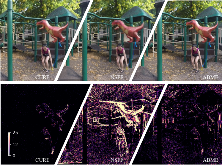
Figure 1: Visual illustration of a frame interpolated by CURE, NSFF [18], and AMBE [34]. NSFF and AMBE are the state-of-the-art methods for dynamic-scene view synthesis and video interpolation, respectively. Note how CURE substantially improves the visual quality and reduces the residual error in the second row.

In this paper, we propose Cross-Video Neural Representation (CURE) as a novel NF method for high-quality temporal video interpolation. Unlike traditional NF methods for representing dynamic scenes, CURE uses a deep neural network to directly represent a video as a continuous function of time and space. This conceptual change significantly simplifies the setup by circumventing the reliance on the camera pose information, which is usually difficult to estimate in certain applications such as handheld filming. The direct application of NF to video interpolation leads to poor performance due to the challenge of representing complex space-time variations from limited data. CURE addresses this issue by introducing a novel strategy based on conditioning the neural field on the input frames using our spatiotemporal encoding module (STEM). For each queried pixel, STEM generates a local feature code that contains the spatial information around the pixel as well as the temporal information from the neighboring frames. STEM thus incorporates a space-time consistency prior into the representation network for mitigating visual artifacts. The architecture of conditioning also allows CURE to learn a video prior across different videos, enabling fast frame interpolation with a simple feed-forward pass. This is fundamentally different from the traditional NF approach of optimizing the weights of neural network for every new test video, thus making the inference computationally expensive.

Contributions: The technical contributions of this work are as follows:

1. We propose CURE as a novel NF approach for temporal video interpolation without any information on the camera pose. CURE is fundamentally different from the existing flow-based and kernel-based DL approaches.

2. We develop a new architecture for CURE that leverages prior information over video frames, thus enforcing plausibility of the synthesized frames. The prior is obtained by conditioning the neural network on local feature codes encoding both temporal and spatial information extracted from the neighboring frames.

3. We perform extensive validation of CURE on several benchmark datasets, including UCF101 [45], Vimeo90K [51], SNU Films [7], Nvidia Dynamic Scene Dataset [52], and Xiph4K. The empirical results show the state-of-the-art performance of CURE for temporal video interpolation as well as highlight its advantage over the current NF methods (see Fig. 1).

2 Related Work

In this section, we briefly review the DL-based methods for video interpolation and discuss several recent results in the area of neural fields.

2.1 Deep Learning for Video Interpolation

A number of DL methods have been developed for video frame interpolation. Early work has proposed direct [23] and phase-base [26] methods that pioneered the usage of deep learning for the task. Recently, the research effort has shifted to flow-based and kernel-based methods due to their improved performance. In the following, we highlight some recent methods from these two classes.

Flow-based methods [22, 12] rely on the optical flow to synthesize new temporal frames by warping the existing frames. A common scheme consists of two modules, where the first module predicts the optical flow and the second module performs frame synthesis. A recent line of work has considered improvements due to the estimation of task-oriented flow in a self-supervised manner [51], leveraging of multiple optical flow maps for characterizing bilateral motion [33, 34], and adoption of recursive multi-scale flow learning [42]. Another line of work has investigated different warping strategies, such as warping both the original frames and their feature representations for extra information [28] and softmax splatting for differentiable forward warping [29].

Kernel-based methods [32] view frame interpolation as convolution operations over local patches. The idea was first introduced in AdaConv [30], which uses spatial-adaptive kernels to capture both the local motion between the input frames and the coefficients for pixel synthesis in the interpolated frame. The empirical success of AdaConv has spurred various follow-up work, including on the use of separable convolutional kernels [31], jointly leveraging optical flow and adaptive convolutions [1], introducing spatiotemporal deformable convolutions [14, 41], and combining channel attention modules [7].

The proposed CURE method represents a new approach based on continuous cross-video neural representation of videos using conditional NF.

2.2 Neural Fields

NF has emerged as a popular vision paradigm with applications in 3D image and shape synthesis [6, 35, 43], tomography [46, 21, 40, 19], audio processing [44], and view rendering [27, 25, 53]. A line of work related to this paper has considered applying NF for view synthesis of dynamic scenes, where the goal is to render a novel image of a temporally-varying scene from an arbitrary viewpoint. Examples include learning a moving human body from sparse multi-view videos [37], jointly learning deformable fields and scenes [18, 8, 36], and 3D video synthesis from multi-view videos [16]. Although these method can be applied for video interpolation (e.g. by fixing the viewpoint in space), they are not designed for this task and usually lead to poor interpolation quality. Another related line of work has applied NF to low-level video processing, including video denoising [8, 4], video super-resolution [8], and video compression [4]. To the best of our knowledge, CURE is the first NF model designed for temporal frame interpolation.

3 Cross-Video Neural Representation

We now present the technical details of CURE. Fig. 3 illustrates the overall structure of the proposed method. We begin by introducing the idea of representing a video segment as a function and then explain the architecture of STEM that infuses the consistency prior into CURE.

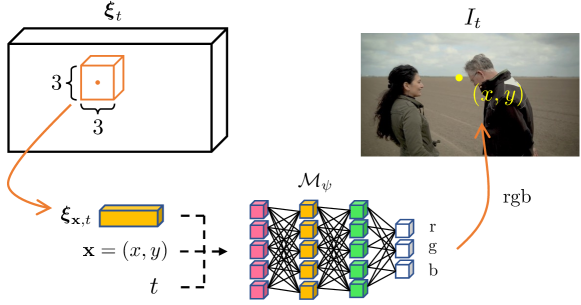
Figure 2: CURE represents a video segment as a continuous vector-valued function, which maps $({\mathbf{x}},t,\boldsymbol{\xi}_{{\mathbf{x}},t})$ to a single RGB color. The vector $\boldsymbol{\xi}_{{\mathbf{x}},t}$ is the local feature code associated with the $3\times 3$ region centered at ${\mathbf{x}}$ for the desired frame $t$.

3.1 Representing Video As a Conditional Neural Field

CURE represents a video segment between two observed frames as a continuous vector-valued function (see the visual illustration in Fig. 2). The input to the function is the spatial pixel location ${\mathbf{x}}=(x,y)\in\mathbb{R}^{2}$, the relative time of the desired frame $0\leq t\leq 1$, and an associated local feature code $\boldsymbol{\xi}_{{\mathbf{x}},t}=\{\xi_{(x-1,y-1,t)},\dots,\xi_{(x+1,y+1,t)}\}$ of the $3\times 3$ region centered at ${\mathbf{x}}$. The output of the function is the single RGB value ${\mathbf{c}}=(r,g,b)\in\mathbb{R}^{3}$ at ${\mathbf{x}}$ in the predicted frame at time $t$. Here, $\xi_{(u,w,\tau)}$ denotes the latent code associated with location $(u,w)$ and time $\tau$, and we selected a $3\times 3$ sub-region in order to impose pixel smoothness. The formulation in CURE does not need any information on the camera pose, simplifying its use. Additionally, the continuous formulation enables CURE to synthesize any frame given by the relative time $t$ (see Fig. 7).

CURE uses a neural network ${\mathcal{M}}_{\psi}:({\mathbf{x}},t,\boldsymbol{\xi}_{{\mathbf{x}},t})\rightarrow\textbf{c}$ to approximate the coordinate-to-function mapping, where the $\psi$ denotes the network weights. The network contains 7 fully-connected layers with 256 neurons. Two skip connections are included in the second and fourth layers to concatenate the input vectors with the intermediate results. Fig. 4(c) shows the architectural details of CURE. It is worth mentioning that as discussed in Sec. 4.3 the exclusion of the spatiotemporal coordinates from CURE leads to suboptimal empirical performance. CURE is trained over multiple videos for learning a general representation of videos. This is achieved by using the neighboring frames to generate the local feature codes. In the experiments, we trained CURE over a standard video interpolation dataset containing frame triplets.

3.2 Spatio-Temporal Encoding

Directly applying NF to video interpolation leads to poor results due to the lack of spatial and temporal consistency. Fig. 8 illustrates the results obtained by the basic NeRF, which simply maps $(x,y,t)$ to the corresponding RGB value. The motivation for spatio-temporal encoding is to provide additional prior information in both space and time to improve the neural representation performance.

We design STEM to generate the local feature codes $\boldsymbol{\xi}_{t}=\{\xi_{(1,1,t)},...,\xi_{(H,W,t)}\}$ from the two neighboring frames $\{I_{0},I_{1}\}$ of the desired frame $I_{t}$. Here, $H$ and $W$ denote pixel width and height of the video. Fig. 3(b) illustrates the detailed architecture of STEM, which we denote as ${\mathcal{S}}_{\theta}:\{I_{0},I_{1}\}\rightarrow\boldsymbol{\xi}_{t}$ for convenience.

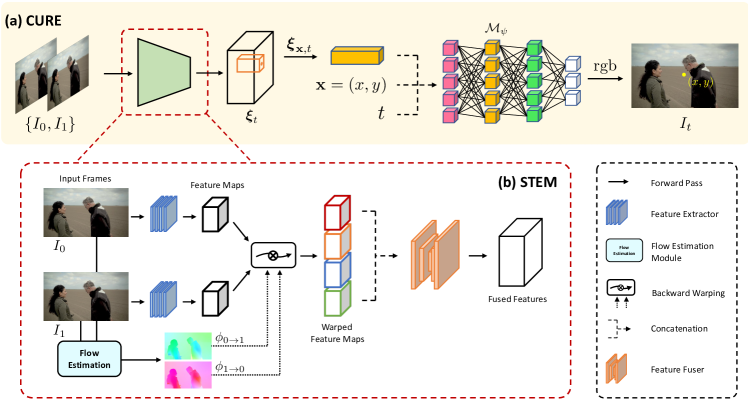
Figure 3: (a) The overall architecture of CURE. (b) The spatiotemporal encoding module (STEM) that generates $\boldsymbol{\xi}_{t}$ for the predicted frame $I_{t}$.

Feature Extraction. STEM first extracts two individual $H\times W\times 64$ feature maps $\{F_{0},F_{1}\}$ from the input frames by using a customized residual network (ResNet) ${\mathcal{R}}:I\rightarrow F$,

$$F_{0}={\mathcal{R}}(I_{0}),\quad F_{1}={\mathcal{R}}(I_{1}).$$ (1)

The architecture of ${\mathcal{R}}$ is shown in Fig. 4(a). Note that these feature maps are later used to form the latent feature map for frame $I_{t}$ via a two-step procedure: feature warping and fusion.

Feature Warping. Feature warping aims to interpolate the latent feature maps associated with time $t$ by warping $\{F_{0},F_{1}\}$. This step ensures the temporal consistency between existing and predicted frames in the latent space. To improve the interpolation accuracy, STEM adopts the bilateral motion approximation technique [33] to generate four bilateral motion maps (fw: forward & bw: backward) from the bidirectional optical flows $\phi_{0\rightarrow 1}$ and $\phi_{1\rightarrow 0}$,

$$\phi_{t\rightarrow 0}^{\text{fw}}=(-t)\times\phi_{0\rightarrow 1},$$ (2a)

$$\phi_{t\rightarrow 1}^{\text{fw}}=(1-t)\times\phi_{0\rightarrow 1},$$ (2b)

$$\phi_{t\rightarrow 0}^{\text{bw}}=t\times\phi_{1\rightarrow 0},$$ (2c)

$$\phi_{t\rightarrow 1}^{\text{bw}}=-(1-t)\times\phi_{1\rightarrow 0}.$$ (2d)

Here, $\phi_{0\rightarrow 1}$ and $\phi_{1\rightarrow 0}$ are estimated by an off-the-shelf differentiable optical flow estimator. In our case, RAFT [48] is used for flow estimation. STEM used the spatial transform network [11] to warp the feature maps. In particular, we warp a target feature map $F_{\text{tar}}$ into a reference feature $F_{\text{ref}}$ by using the motion map from the reference to target

$$F_{\text{ref}}({\mathbf{x}})=F_{\text{tar}}({\mathbf{x}}+\phi_{\text{ref}\rightarrow\text{tar}}({\mathbf{x}}))$$ (3)

By applying (3) and (2) to $\{F_{0},F_{1}\}$, we can obtain four warped feature maps via cross combination

$$F_{0\rightarrow t}^{\text{bw}}({\mathbf{x}})=F_{0}({\mathbf{x}}+\phi^{\text{bw}}_{t\rightarrow 0}({\mathbf{x}})),$$ (4a)

$$F_{1\rightarrow t}^{\text{bw}}({\mathbf{x}})=F_{1}({\mathbf{x}}+\phi^{\text{bw}}_{t\rightarrow 1}({\mathbf{x}})),$$ (4b)

$$F_{0\rightarrow t}^{\text{fw}}({\mathbf{x}})=F_{0}({\mathbf{x}}+\phi^{\text{fw}}_{t\rightarrow 0}({\mathbf{x}})),$$ (4c)

$$F_{1\rightarrow t}^{\text{fw}}({\mathbf{x}})=F_{1}({\mathbf{x}}+\phi^{\text{fw}}_{t\rightarrow 1}({\mathbf{x}})),$$ (4d)

where a single warped feature map has the spatial dimension of $H\times W\times 64$. In feature warping, STEM adopted bilinear interpolation to handle off-the-grid pixels.

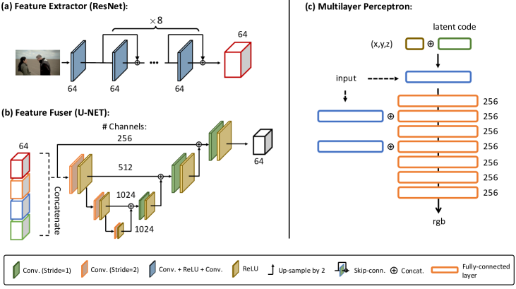
Figure 4: Visual illustration of the network architectures used in CURE.

Feature Fusion. To output the final local feature codes for $I_{t}$, a feature fusion step is then employed to fuse the warped feature maps into a single $H\times W\times 64$ feature map,

$$\boldsymbol{\xi}_{t}={\mathcal{U}}(F_{\text{concat}})$$ (5)

where $$F_{\text{concat}}\,\coloneqq\,F^{\text{fw}}_{0\rightarrow t}\oplus F^{\text{fw}}_{1\rightarrow t}\oplus F^{\text{bw}}_{0\rightarrow t}\oplus F^{\text{bw}}_{1\rightarrow t}.$$

Here, $\oplus$ denotes feature concatenation along the channel dimension, and ${\mathcal{U}}$ represents the fusion network. In STEM, we implemented a customized U-Net as ${\mathcal{U}}$, which is shown in Fig 4(b).

3.3 Training of CURE

We jointly optimize the parameters of STEM and the coordinate-based neural network by minimizing the mean squared error (MSE) for each pixel location

$${\mathcal{L}}(\psi,\theta)=\|{\mathcal{M}}_{\psi}({\mathbf{x}},t,\boldsymbol{\xi}_{{\mathbf{x}},t})-I_{t}({\mathbf{x}})\|_{2}^{2}\quad\text{where}\quad\boldsymbol{\xi}_{t}={\mathcal{S}}_{\theta}(I_{0},I_{1}).$$ (6)

The vector $\theta$ includes the weights of the feature extraction network ${\mathcal{R}}$, feature fusion network ${\mathcal{U}}$, and the optical flow estimator RAFT. We initialize RAFT with the default pre-trained weights, and set the RAFT iteration number to $50$.

We trained CURE on the training dataset Vimeo90K [51]. We performed data augmentation by vertically and horizontally flipping the video frames. CURE is trained by taking the start and end frames as input and predicting the middle frame at $t=0.5$. Once trained, CURE can continuously interpolate frames at any $t\in(0,1)$ (see Fig. 7). We used Adam [13] optimizer to optimize all network parameters for 70 epochs. We implemented a diminishing learning rate which decreases by 0.95 at every epoch. The training was performed on a machine equipped with an AMD Ryzen Threadripper 3960X 24-Core Processor and 2 NVIDIA GeForce RTX 3090 GPUs. It took roughly 3 weeks to train the model.

4 Experiments

We numerically validated CURE on several standard video interpolation datasets. Our experiments include comparisons with the state-of-the-art (SOTA) methods and ablation studies highlighting the key components of the proposed architecture.

4.1 Datasets

We consider the following four datasets for numerical evaluation:

Vimeo90K: The Vimeo90K training dataset contains 51,312 frame triplets with $448\times 256$ pixel resolution, and the validation dataset contains 3,782 triplets that we use for testing. We additionally increased the training data by extracting 91,701 triplets (i.e. $\{I_{0},I_{2},I_{4}\}$) from the septulets dataset.

UCF101: The UCF101 [45] dataset contains realistic action videos collected from YouTube. We used a subset collected by [22] for evaluation. The subset contains 379 triplets with $256\times 256$ resolution.

SNU-FILM: The dataset [7] contains $1,240$ triplets extracted from different videos with up to $1280\times 720$ resolution. The triplets are categorized to easy, medium, hard, and extreme, based on the motion strength between frames.

Xiph4K: The dataset contains eight randomly-selected 4K videos downloaded from the Xiph website. For each video, we extracted the first fifty odd-numbered frames to form the testing triplets, all resized to $2048\times 1080$ pixels.

Nvidia Dynamic Scene (ND Scene): ND Scene [52] is a video dataset that is commonly used for novel view synthesis. The dataset contains videos of eight scenes, recorded by a static camera rig with twelve GoPro cameras. We separate each video into triplets with a temporal sliding window of three frames.

X4K: The X4K dataset [42] contains eight 4K videos with 33 frames. We used this dataset for testing continuous multi-frame interpolation, with all videos resized to $2048\times 1080$ pixels. In the test, we used the first and last frames as input frames to predict seven middle frames, that is, $\{I_{4},I_{8},I_{12},I_{15},I_{20},I_{24},I_{28}\}$.

Quantitative Metrics: We use peak-signal-to-noise ratio (PSNR) and structural similarity index (SSIM) to quantify the performance of all methods.

Table 1: Average PSNR/SSIM obtained by CURE and the current state-of-the-art (SOTA) methods on UCF101, Vimeo90K, and SNU-FILM, NDScene, and Xiph4K datasets. We use bold and underline to highlight the highest and second highest values, respectively. Note the superior results of CURE over SOTA methods.

	UCF 101	Vimeo 90K	SNU-FILM				ND Scene	Xiph4K	Average
			Easy	Medium	Hard	Extreme
lightgraySepConv [31] (ICCV17)	27.97 0.9401	27.32 0.9481	30.33 0.9661	27.33 0.9451	22.80 0.8794	18.06 0.7747	24.38 0.9294	22.83 0.9748	25.13 0.9072
ToFlow [51] (IJCV19)	34.58 0.9667	33.73 0.9682	39.08 0.9890	34.39 0.9740	28.44 0.9180	23.39 0.8310	30.05 0.9466	27.53 0.9850	31.40 0.9361
lightgrayBMBC [33] (ECCV20)	35.16 0.9689	35.01 0.9764	39.90 0.9902	35.31 0.9774	29.33 0.9270	23.92 0.8432	36.01 0.9827	28.03 0.9131	32.83 0.9474
CAIN [7] (AAAI20)	34.91 0.9690	34.65 0.9730	39.89 0.9900	35.61 0.9776	29.90 0.9292	24.78 0.8507	34.81 0.9789	29.94 0.9184	33.06 0.9484
lightgrayRRIN [15] (ICASSP20)	34.93 0.9496	35.22 0.9643	39.31 0.9897	35.23 0.9776	29.79 0.9301	24.59 0.8511	33.89 0.9750	29.30 0.9232	32.78 0.9451
AdaCoF [14] (CVPR20)	34.90 0.9680	34.47 0.9730	39.80 0.9900	35.05 0.9754	29.46 0.9244	24.31 0.8439	35.75 0.9822	28.57 0.9093	32.79 0.9458
lightgrayXVFI [42] (ICCV21)	35.09 0.9685	35.07 0.9760	39.76 0.9991	35.12 0.9769	29.30 0.9245	23.98 0.8417	35.76 0.9819	28.46 0.9121	32.82 0.9476
ABME [34] (ICCV21)	35.38 0.9698	36.18 0.9805	39.59 0.9901	35.77 0.9789	30.58 0.9364	25.42 0.8639	33.17 0.9736	30.74 0.9366	33.35 0.9537
CURE	35.36 0.9705	35.73 0.9789	39.90 0.9910	35.94 0.9797	30.66 0.9373	25.44 0.8638	36.24 0.9839	30.94 0.9389	33.78 0.9555

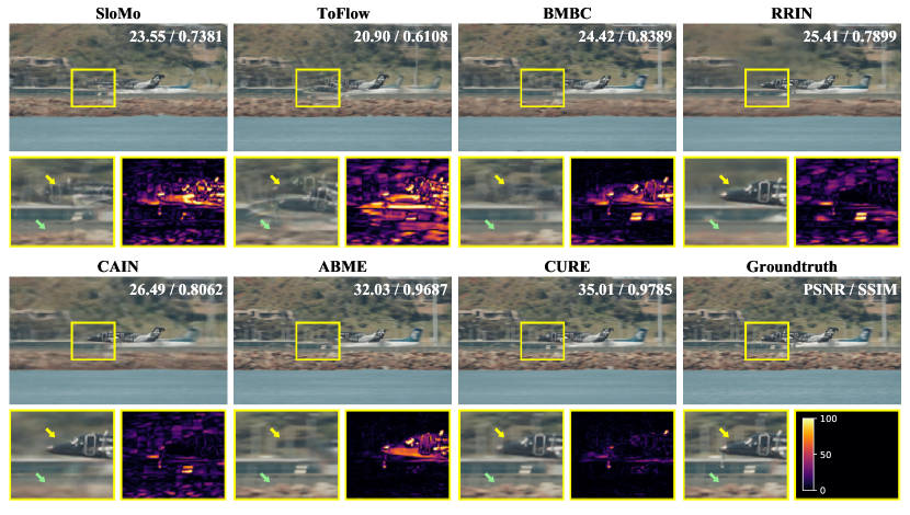
Figure 5: Visual comparison between CURE and current SOTA methods on an example from Vimeo90K. The visual differences are highlight by the yellow boxes paired with the residual error maps. Note how CURE outperforms the SOTA methods in term of sharpness (see green arrows) and accuracy (yellow arrows).

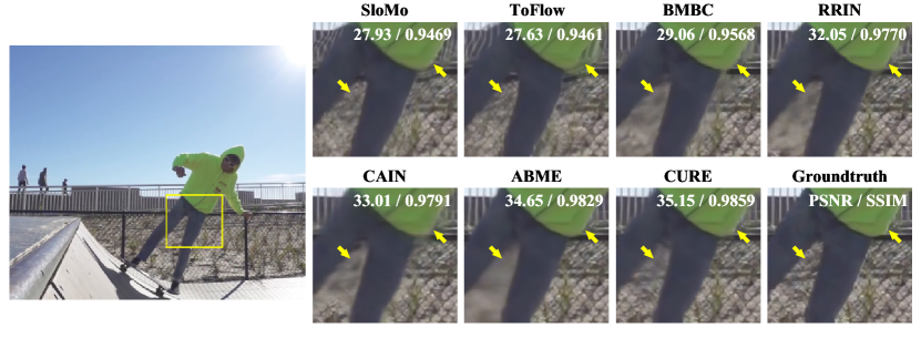
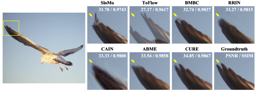
Figure 6: Visual comparison between CURE and current SOTA methods on two examples from SNU-FILM (hard). We highlight the differences by zooming in the regions with the presence of strong motion (the man’s waist and the bird’s wingtip). Note how CURE outperforms the SOTA methods by removing distortions and enhancing sharpness.

4.2 Performance Evaluation

Comparison with video interpolation methods. Table 1 summarizes the results of comparing CURE against several SOTA algorithms. The results are obtained by running the published code with the pre-trained weights. The average PSNR and SSIM values obtained by each algorithm on the considered datasets are presented. Note how CURE outperforms all SOTA methods in terms of the PSNR/SSIM values averaged over all datasets. For example, CURE outperforms ABME, which is the latest SOTA method, on most datasets and tied its performance (i.e. -0.1 dB in PSNR or -0.001 in SSIM) on the rest.

Table 2: Avg. PSNR/SSIM values obtained on X4K.

Methods	X4K
lightgraySuperSloMo	19.58 / 0.7099
ToFlow	22.33/0.7259
lightgrayBMBC	24.28 / 0.7777
XVFI	24.12/0.7566
lightgrayCURE	30.05 / 0.8998

Fig. 5 visually compares CURE to several representative SOTA methods on an example from Vimeo90K. We highlight the visual differences by zooming in the yellow box and plotting the corresponding residual error map. In this comparison, SloMO, ToFlow, and BMBC reconstruct video frames with significant blurry and ghosting artifacts, failing to capture the shape of the airplane front (see yellow arrows). While RRIN and CAIN successfully recover the airplane front, they completely blur the mountain in the background (see green arrows). Note how CURE clearly reconstructs both the moving airplane as well as the background mountain with fine details. The qualitative visual improvements are also corroborated by the higher quantitative values and lower residual errors.

Fig. 6 provides a visual results on two videos from SNU-FILM (hard). These two examples were selected due to the fast motion of the recorded objects, which makes the frame interpolation challenging. ToFlow completely fails to reconstruct the bird’s wingtip in the second video. Other algorithms, such as BMBC, RRIN, CAIN, and AMBE, produce blurry frames that smooth out the details on the feathers. CURE successfully handles the motion by reconstructing a sharp frame. Note the visual similarity between the frame synthesized by CURE and the groundtruth. Similar results can be observed in the comparison on the first video of a man skateboarding, where CURE significantly outperforms other algorithms.

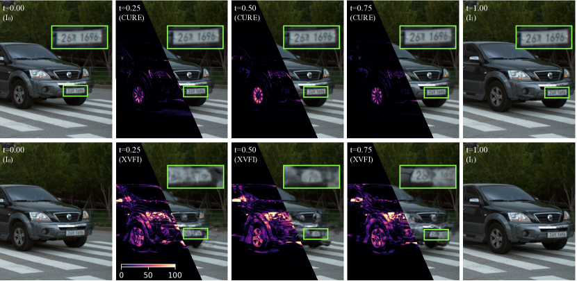
Figure 7: Visual demonstration of the continuous interpolation by CURE on an example from the X4K dataset. Only two frames $\{I_{0},I_{1}\}$ are used for predicting several middle frames at temporal locations $t\in\{0.25,0.5,0.75\}$. Note the sharp textural details preserved by CURE, but lost in the results by XVFI.

Fig. 7 highlights CURE’s ability to perform continuous interpolation on a challenging video from X4K. We include the result by XVFI as the baseline. Each figure plots both image and the corresponding residual error map with respect to the groundtruth. The visual differences on the textural details are highlighted in the green boxes. Note that both CURE and XVFI were only trained to predict the frame at $t=0.5$ on the Vimeo90K dataset. CURE produces high-quality and accurate frames for every temporal location, significantly outperforming XVFI in terms of both visual quality and precision. Note how CURE recovers the vehicle license plate that is completely distorted by XVFI. Corresponding quantitative results are summarized in Table 2, corroborating the excellent performance of CURE.

Comparison with NF methods. We compared CURE with two different NF algorithms: (1) vanilla NF (V-NF) that directly learns a coordinate-based neural network to map $({\mathbf{x}},t)$ to the corresponding color pixel, and (2) NSFF [18] that learns the dynamic scene in the video and applies view synthesis to generate new frames. Both algorithms need to re-optimize their weights for every test video/scene, while CURE learns a general video prior. We implemented V-NF by adopting the neural network architecture of NeRF and setting the positional encoding $L$ to 10 and 2 for $(x,y)$ and $t$, respectively. We trained V-NF by using the even-number frames. For NSFF, we downloaded the pre-trained models for testing. Note that these comparisons are provided for completeness only; the performance of these NF algorithms on video interpolation should not be interpreted as an indication of their performance on their original tasks.

We evaluated the comparison on ND Scene. For each scene, we randomly selected one camera video from the videos captured by twelve cameras. We resized each video to accommodate the setup used by the pre-trained models of NSFF. Table 3 summarizes the details and quantitative results on each test video. As illustrated, CURE significantly outperforms V-NF and NSFF in every test scenario, and the PSNR improvement is usually over 5 dB. Fig. 8 presents a visual comparison of the truck video to better highlight the difference.Without any consistency constraint, V-NF faithfully recovers the general content in the frame, but loses the feature details and suffers strong gridding artifacts. For example, the residual map highlights the missing edges in the interpolated frame in V-NF. On the other hand, NSFF generates a visually pleasing frame with faithful details. However, the problem of NSFF is that it predicts the wrong position of the moving truck, which significantly reduces the PSNR values. CURE avoids all these problems and interpolates a high-quality frame with both fine details and correct position of the truck. These results highlight the contribution of CURE to the research on NF-based video frame interpolation.

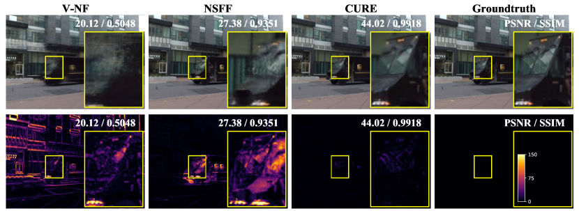
Figure 8: Visual comparison between CURE, vanilla-NeRF, and NSFF methods on ND Scene. The first row shows the images, and the second row shows the corresponding residual error map. We highlighted the visual difference in the yellow box. CURE achieves substantially higher PSNR (about 17 dB) over NSFF.

Table 3: Quantitative (PSNR/SSIM) comparisons of different video representation algorithms on the ND Scene dataset. This table highlights that CURE provides better video representation by learning a general prior across videos.

Dataset	Camera Post	Resolution	Algorithms
			V-NF	NSFF [18]	CURE
lightgray Ballon1-2	1	$540\times 288$	10.75/0.4582	24.58/0.8980	31.05/0.9742
Dynamic Face-2	3	$547\times 288$	23.09/0.8317	27.13/0.9608	40.81/0.9930
lightgrayJumping	5	$540\times 288$	26.07/0.8099	27.19/0.9281	31.23/0.9624
Playground	2	$573\times 288$	22.45/0.7222	24.64/0.8912	36.15/0.9938
lightgraySkating-2	4	$541\times 288$	28.44/0.8648	34.05/0.9782	39.67/0.9899
Truck-2	9	$542\times 288$	28.37/0.8075	34.74/0.9751	39.78/0.9887
lightgrayUmbrella	11	$543\times 288$	23.91/0.5876	23.91/0.8441	39.66/0.9880

4.3 Ablation Studies

We highlighted the key components of the proposed model by conducting several ablation experiments. We focus on showing the effectiveness of the coordinate-based neural representation by considering two baseline variants:

CURE-w/o-Rep: This method directly trains the STEM network as a frame interpolator by adding an additional head to predict the RGB images. We design CURE-w/o-Rep to show the importance of the NF module.

CURE-w/o-Crd: This method simplifies CURE by removing the input of the spatiotemporal coordinate $({\mathbf{x}},t)$. We design CURE-w/o-Crd to show the importance of the coordinate indexing for synthesizing the desired RGB values.

Fig. 9 visually compares CURE with its two baseline variants on an example from SNU (hard). Without neural representation, CURE-w/o-Rep predicts the wrong location of the bird’s wingtip shown in the green box, losing enough representation power to properly represent the video. On the other hand, CURE-w/o-Crd produces a blurry image that loses the texture details by missing the exact spatiotemporal coordinate. Table 4 summarizes the numerical values on all the considered datasets. The results clearly show that CURE achieves the best results by jointly leveraging STEM and coordinate-based representation.

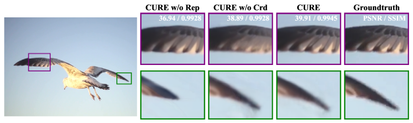
Figure 9: Visual illustration of the importance of the various components of CURE. The green and yellow boxes highlight the improvements in terms of accuracy and sharpness due to the full CURE compared to its ablated variants.

Table 4: Average PSNR/SSIM obtained by the full CURE and its ablated variants.

	UCF 101	Vimeo 90K	SNU-FILM				ND Scene	Xiph4K	Average
			Easy	Medium	Hard	Extreme
lightgray CURE w/o Rep	34.80 0.9682	35.15 0.9769	39.82 0.9903	35.71 0.9787	30.36 0.9350	25.14 0.8601	35.13 0.9802	30.45 0.9359	33.32 0.9530
CURE w/o Crd	35.11 0.9689	35.25 0.9772	39.76 0.9900	35.63 0.9784	30.39 0.9350	25.26 0.8609	35.68 0.9816	30.52 0.9341	33.45 0.9531
CURE	35.36 0.9705	35.73 0.9789	39.90 0.9910	35.94 0.9797	30.66 0.9373	25.44 0.8638	36.24 0.9839	30.94 0.9389	33.78 0.9555

5 Conclusion

This work proposes a novel temporal video frame interpolation algorithm, CURE, which is based on the recent class of techniques known as neural fields (NF). The key idea of CURE is to represent video segment between two observed frames as a continuous vector-valued function of the spatiotemporal coordinates, which is parameterized by a fully-connected coordinate-based neural network. Unlike the traditional NF variants, CURE enforces space-time consistency in the synthesized frames by conditioning its NF on the information from the neighboring frames. This conditioning enables CURE to learn a prior across different videos. Experimental evaluations clearly show that the CURE outperforms the state-of-the-art methods on five benchmark datasets. The comparisons with the traditional NF methods and with the ablated variants of CURE highlight the synergistic effect of various components of the full CURE.

References

- [1] W. Bao, W. S. Lai, X. Zhang, Z. Gao, and M. H. Yang. MEMC-Net: Motion estimation and motion compensation driven neural network for video interpolation and enhancement. IEEE Transactions on Pattern Analysis and Machine Intelligence, 43(3):933–948, 2021.
- [2] T. Brox, A. Bruhn, N. Papenberg, and J. Weickert. High accuracy optical flow estimation based on a theory for warping. In European Conference on Computer Vision, pages 25–36. Springer, 2004.
- [3] R Castagno, P. Haavisto, and G. Ramponi. A method for motion adaptive frame rate up-conversion. IEEE Transactions on circuits and Systems for Video Technology, 6(5):436–446, 1996.
- [4] H. Chen, B. He, H. Wang, Y. Ren, S. N. Lim, and A. Shrivastava. NeRV: Neural representations for videos. In Advances in Neural Information Processing Systems, 2021.
- [5] Z. Chen, H. Jin, Z. Lin, S. Cohen, and Y. Wu. Large displacement optical flow from nearest neighbor fields. In Proceedings of the IEEE Conference on Computer Vision and Pattern Recognition, pages 2443–2450, 2013.
- [6] Z. Chen and H. Zhang. Learning implicit fields for generative shape modeling. In Proceedings of the IEEE Conference on Computer Vision and Pattern Recognition, pages 5939–5948, 2019.
- [7] M. Choi, H. Kim, B. Han, N. Xu, and K. M. Lee. Channel attention is all you need for video frame interpolation. In Proceedings of the AAAI Conference on Artificial Intelligence, volume 34, pages 10663–10671, 2020.
- [8] Y. Du, Y. Zhang, H. X. Yu, J. B. Tenenbaum, and J. Wu. Neural radiance flow for 4D view synthesis and video processing. In Proceedings of the IEEE/CVF International Conference on Computer Vision, pages 14324–14334, 2021.
- [9] J. Flynn, I. Neulander, J. Philbin, and N. Snavely. DeepStereo: Learning to predict new views from the world’s imagery. In Proceedings of the IEEE Conference on Computer Vision and Pattern Recognition, pages 5515–5524, 2016.
- [10] T. W. Hui, X. Tang, and C. C. Loy. LiteFlowNet: A lightweight convolutional neural network for optical flow estimation. In Proceedings of the IEEE Conference on Computer Vision and Pattern Recognition, pages 8981–8989, 2018.
- [11] M. Jaderberg, K. Simonyan, A. Zisserman, et al. Spatial transformer networks. Advances in Neural Information Processing Systems, 28, 2015.
- [12] D. Jiang, H.and Sun, V. Jampani, M. H. Yang, E. Learned-Miller, and J. Kautz. SuperSloMo: High quality estimation of multiple intermediate frames for video interpolation. In Proceedings of the IEEE Conference on Computer Vision and Pattern Recognition, pages 9000–9008, 2018.
- [13] D. Kingma and J. Ba. Adam: A method for stochastic optimization. In International Conference on Learning Representations (ICLR), 2015.
- [14] H. Lee, T. Kim, T. Y. Chung, D. Pak, Y. Ban, and S. Lee. AdaCof: adaptive collaboration of flows for video frame interpolation. In Proceedings of the IEEE/CVF Conference on Computer Vision and Pattern Recognition, pages 5316–5325, 2020.
- [15] H. Li, Y. Yuan, and Q. Wang. Video frame interpolation via residue refinement. In IEEE International Conference on Acoustics, Speech and Signal Processing (ICASSP), pages 2613–2617, 2020.
- [16] T. Li, M. Slavcheva, M. Zollhoefer, S. Green, C. Lassner, C. Kim, T. Schmidt, S. Lovegrove, M. Goesele, and Z. Lv. Neural 3D video synthesis. arXiv:2103.02597, 2021.
- [17] Z. Li, S. Niklaus, N. Snavely, and O. Wang. Neural scene flow fields for space-time view synthesis of dynamic scenes. arXiv:2011.13084, 2020.
- [18] Z. Li, S. Niklaus, N. Snavely, and O. Wang. Neural scene flow fields for space-time view synthesis of dynamic scenes. In Proceedings of the IEEE/CVF Conference on Computer Vision and Pattern Recognition, pages 6498–6508, 2021.
- [19] D. B. Lindell, J. N. P. Martel, and G. Wetzstein. AutoInt: automatic integration for fast neural volume rendering. In Proceedings of the IEEE/CVF Conference on Computer Vision and Pattern Recognition, 2021.
- [20] L. Liu, J. Gu, K. Z. Lin, T. S. Chua, and C. Theobalt. Neural sparse voxel fields. Advances in Neural Information Processing Systems, 33:15651–15663, 2020.
- [21] R. Liu, Y. Sun, J. Zhu, L. Tian, and U. S. Kamilov. Zero-shot learning of continuous 3D refractive index maps from discrete intensity-only measurements. arXiv:2112.00002, 2021.
- [22] Z. Liu, R. A Yeh, X. Tang, Y. Liu, and A. Agarwala. Video frame synthesis using deep voxel flow. In Proceedings of the IEEE International Conference on Computer Vision, pages 4463–4471, 2017.
- [23] G. Long, L. Kneip, J. M Alvarez, H. Li, X. Zhang, and Q. Yu. Learning image matching by simply watching video. In European Conference on Computer Vision, pages 434–450, 2016.
- [24] G. Lu, X. Zhang, L. Chen, and Z. Gao. Novel integration of frame rate up conversion and hevc coding based on rate-distortion optimization. IEEE Transactions on Image Processing, 27(2):678–691, 2017.
- [25] R. Martin-Brualla, N. Radwan, M. SM Sajjadi, J. T Barron, A. Dosovitskiy, and D. Duckworth. NeRF in the wild: Neural radiance fields for unconstrained photo collections. In Proceedings of the IEEE Conference on Computer Vision and Pattern Recognition, pages 7210–7219, 2021.
- [26] S. Meyer, A. Djelouah, B. McWilliams, A. Sorkine-Hornung, M. Gross, and C. Schroers. Phasenet for video frame interpolation. In Proceedings of the IEEE Conference on Computer Vision and Pattern Recognition, pages 498–507, 2018.
- [27] B. Mildenhall, P. P. Srinivasan, M. Tancik, J. T. Barron, R. Ramamoorthi, and R. Ng. NeRF: Representing scenes as neural radiance fields for view synthesis. In European Conference on Computer Vision, pages 405–421, 2020.
- [28] S. Niklaus and F. Liu. Context-aware synthesis for video frame interpolation. In Proceedings of the IEEE Conference on Computer Vision and Pattern Recognition, pages 1701–1710, 2018.
- [29] S. Niklaus and F. Liu. Softmax splatting for video frame interpolation. In Proceedings of the IEEE/CVF Conference on Computer Vision and Pattern Recognition, pages 5437–5446, 2020.
- [30] S. Niklaus, L. Mai, and F. Liu. Video frame interpolation via adaptive convolution. In Proceedings of the IEEE Conference on Computer Vision and Pattern Recognition, pages 670–679, 2017.
- [31] S. Niklaus, L. Mai, and F. Liu. Video frame interpolation via adaptive separable convolution. In Proceedings of the IEEE International Conference on Computer Vision, pages 261–270, 2017.
- [32] S. Niklaus, L. Mai, and O. Wang. Revisiting adaptive convolutions for video frame interpolation. In Proceedings of the IEEE/CVF Winter Conference on Applications of Computer Vision, pages 1099–1109, 2021.
- [33] J. Park, K. Ko, C. Lee, and C. S. Kim. BMBC: Bilateral motion estimation with bilateral cost volume for video interpolation. In European Conference on Computer Vision, pages 109–125, 2020.
- [34] J. Park, C. Lee, and C. S. Kim. Asymmetric bilateral motion estimation for video frame interpolation. In Proceedings of the IEEE/CVF International Conference on Computer Vision, pages 14539–14548, 2021.
- [35] J. J. Park, P. Florence, J. Straub, Ri. Newcombe, and S. Lovegrove. DeepSDF: Learning continuous signed distance functions for shape representation. In Proceedings of the IEEE Conference on Computer Vision and Pattern Recognition, pages 165–174, 2019.
- [36] K. Park, U. Sinha, J. T Barron, S. Bouaziz, D. B Goldman, S. M Seitz, and R. Martin-Brualla. Nerfies: Deformable neural radiance fields. In Proceedings of the IEEE/CVF International Conference on Computer Vision, pages 5865–5874, 2021.
- [37] S. Peng, Y. Zhang, Y. Xu, Q. Wang, Q. Shuai, H. Bao, and X. Zhou. Neural body: Implicit neural representations with structured latent codes for novel view synthesis of dynamic humans. In Proceedings of IEEE Conference Computer Vision and Pattern Recognition, 2021.
- [38] A. Ranjan and M. J Black. Optical flow estimation using a spatial pyramid network. In Proceedings of the IEEE Conference on Computer Vision and Pattern Recognition, pages 4161–4170, 2017.
- [39] Z. Ren, J. Yan, B. Ni, B. Liu, X. Yang, and H. Zha. Unsupervised deep learning for optical flow estimation. In Proceedings of the AAAI Conference on Artificial Intelligence, volume 31, 2017.
- [40] L. Shen, J. Pauly, and L. Xing. NeRP: implicit neural representation learning with prior embedding for sparsely sampled image reconstruction. arXiv:2108.10991 [eess.IV], 2021.
- [41] Z. Shi, X. Liu, K. Shi, L. Dai, and J. Chen. Video frame interpolation via generalized deformable convolution. IEEE Transactions on Multimedia, 2021.
- [42] H. Sim, J. Oh, and M. Kim. XVFI: Extreme video frame interpolation. In Proceedings of the IEEE/CVF International Conference on Computer Vision, pages 14489–14498, 2021.
- [43] V. Sitzmann, J. Martel, A. Bergman, D. Lindell, and G. Wetzstein. Implicit neural representations with periodic activation functions. In Advances in Neural Information Processing Systems, volume 33, 2020.
- [44] V. Sitzmann, M. Zollhoefer, and G. Wetzstein. Scene representation networks: Continuous 3d-structure-aware neural scene representations. In Advances in Neural Information Processing Systems, volume 32, 2019.
- [45] K. Soomro, A. R. Zamir, and M. Shah. Ucf101: A dataset of 101 human actions classes from videos in the wild. arXiv preprint arXiv:1212.0402, 2012.
- [46] Y. Sun, J. Liu, M. Xie, B. Wohlberg, and U. S. Kamilov. Coil: Coordinate-based internal learning for tomographic imaging. IEEE Trans. Comp. Imag., pages 1–1, 2021.
- [47] H. Takeda, P. Van Beek, and P. Milanfar. Spatio-temporal video interpolation and denoising using motion-assisted steering kernel (mask) regression. In Proceedings of the IEEE International Conference on Image Processing, pages 637–640, 2008.
- [48] Z. Teed and J. Deng. RAFT: recurrent all-pairs field transforms for optical flow. In European Conference on Computer Vision, pages 402–419. Springer, 2020.
- [49] J. Wu, C. Yuen, N. M. Cheung, J. Chen, and C. W. Chen. Modeling and optimization of high frame rate video transmission over wireless networks. IEEE Transactions on Wireless Communications, 15(4):2713–2726, 2015.
- [50] W. Xian, J. B. Huang, J. Kopf, and C. Kim. Space-time neural irradiance fields for free-viewpoint video. In Proceedings of the IEEE/CVF Conference on Computer Vision and Pattern Recognition, pages 9421–9431, 2021.
- [51] T. Xue, B. Chen, J. Wu, D. Wei, and W. T. Freeman. Video enhancement with task-oriented flow. International Journal of Computer Vision, 127(8):1106–1125, 2019.
- [52] J. S. Yoon, K. Kim, O. Gallo, H. S. Park, and J. Kautz. Novel view synthesis of dynamic scenes with globally coherent depths from a monocular camera. In Proceedings of the IEEE/CVF Conference on Computer Vision and Pattern Recognition, pages 5336–5345, 2020.
- [53] K. Zhang, G. Riegler, N. Snavely, and V. Koltun. NeRF++: Analyzing and improving neural radiance fields. arXiv:2010.07492 [cs.CV], 2020.