An Achievable Rate Region for $3-$User Classical-Quantum Broadcast Channels

Abstract

We consider the scenario of communicating on a $3\mathchar 45\relax$user classical-quantum broadcast channel. We undertake an information theoretic study and focus on the problem of characterizing an inner bound to its capacity region. We design a new coding scheme based partitioned coset codes - an ensemble of codes possessing algebraic properties. Analyzing its information-theoretic performance, we characterize a new inner bound. We identify examples for which the derived inner bound is strictly larger than that achievable using IID random codes.

I Introduction

We consider the scenario of communicating on a $3\mathchar 45\relax$user classical-quantum broadcast channel ($3\mathchar 45\relax$CQBC) depicted in Fig. 1. Our focus is on the problem of designing an efficient coding scheme and characterizing an inner bound (achievable rate region) to the capacity region of a general $3\mathchar 45\relax$CQBC. The current known coding schemes [1, 2, 3] for CQBCs are based on conventional IID random codes, also referred to herein as unstructured codes. In this work, we undertake a study of coding schemes based on coset codes for CQBC communication and present the following contributions.

We propose a new coding scheme based on partitioned coset codes (PCC) - an ensemble of codes possessing algebraic closure properties. We analyze its performance to derive a new inner bound to the capacity region of a general $3\mathchar 45\relax$CQBC. We identify examples of $3\mathchar 45\relax$CQBCs for which the derived inner bound is strictly larger than the current known largest. Our findings maybe viewed as another step [4, 5] in our pursuit of designing coding schemes based on coset codes for network CQ communication, and in particular, a first step in deriving a new achievable rate region for a general $3\mathchar 45\relax$CQBC.

An information theoretic study of CQBCs was initiated by Yard et. al. [1] in the context of $2\mathchar 45\relax$CQBCs wherein the superposition coding scheme was studied. Furthering this study, Savov and Wilde [2] proved achievability of Marton’s binning [6] for a general $2\mathchar 45\relax$CQBC. While these studied the asymptotic regime, Radhakrishnan et. al. [3] proved achievability of Marton’s inner bound [6] in the one-shot regime which also extended to clear proofs for the former regime considered in [1, 2].

The works [1, 2, 3] were aimed at generalizing Marton’s classical coding [6] schemes that is based on IID codes. Fueled by the simplicity of IID codes and more importantly, a lack of evidence for their sub-optimality in one-to-many communication scenarios, most studies of the broadcast channel (BC) problem have restricted attention to IID coding schemes. Indeed, even within the larger class of BCs that include continuous valued sets, any number of receivers (Rxs) and multiple antennae, we were unaware of any BC for which IID coding schemes were sub-optimal. In 2013, [7] identified a $3\mathchar 45\relax$user classical BC ($3\mathchar 45\relax$CBC) for which a linear coding scheme strictly outperforms even a most general IID coding scheme that incorporates all known strategies [8, 6, 9]. This article builds on the ideas in [10] and is driven by a motivation to elevate the same to $3\mathchar 45\relax$CQBCs. In the sequel, we discuss why codes endowed with algebraic closure properties can enhance one-to-many communication.

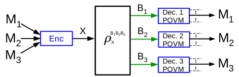
Figure 1: Communicating classical information over a $3\mathchar 45\relax$CQBC.

Communication on a BC entails fusing codewords chosen for the different Rxs through a single input. From the perspective of any Rx, a specific aggregation of the codewords chosen for the other Rxs acts as interference. See Fig. 2. The Tx can precode for this interference via Marton’s binning. In general, precoding entails a rate loss. In other words, suppose $W$ is the interference seen by Rx $1$, then the rate that Rx $1$ can achieve by decoding $W$ and peeling it off can be strictly larger than what it can achieve if the Tx precodes for $W$. This motivates every Rx to decode as large a fraction of the interference that it can and precode only for the minimal residual uncertainty.

In contrast to a BC with $2$ Rxs, the interference $W$ on a BC with $3$ Rxs is a bivariate function of $V_{2},V_{3}$ - the signals of the other Rxs (Fig. 2). A joint design of the $V_{2}\mathchar 45\relax,V_{3}\mathchar 45\relax$codes endowing them with structure can enable Rx $1$ decode $W$ efficiently even while being unable to decode $V_{2}$ and $V_{3}$. We elaborate on this phenomena through chosen examples (Ex. 1, 2) followed by a self contained discussion that informs us of the structure (Sec. III-A) of a general coding scheme.

In this article, we present our first inner bound (Thm. 1) that illustrates several of the new elements - code structure, decoding rule and analysis steps. This coding scheme equips each user with just one codebook. Rx $1$ decodes a bivariate function of the interference while Rxs $2$ and $3$ only decode into their codebooks. A general coding scheme for a $3-$CQBC must permit precoding and message splitting to enable each Rx decode both univariate and bivariate components of signals intended for the other Rxs. As elaborated in the context of a $3\mathchar 45\relax$CBC [10, Sec. IV], this involves multiple codebooks. We refer the reader to [11] wherein further steps in enlarging the inner bound derived in Thm. 1 are provided. Even while, Thm. 1 is a first step, Prop. 1 identifies examples for which it is strictly larger.

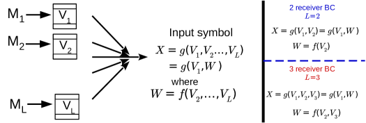
Figure 2: From Rx $1$’s perspective, the interference $W$ it experiences is a specific combination of the other user codewords. While on $2\mathchar 45\relax$user BC, $W$ is a univariate function of $V_{2}$, on a $3\mathchar 45\relax$user, $W$ is a bi-variate function of $V_{2},V_{3}$

II Preliminaries and Problem Statement

For $n\in\mathbb{N}$, $[n]\mathrel{\ensurestackMath{\stackon[1pt]{=}{\scriptstyle\Delta}}}\left\{1,\cdots,n\right\}$. For a Hilbert space $\mathcal{H}$, $\mathcal{L}(\mathcal{H}),\mathcal{P}(\mathcal{H})$ and $\mathcal{D}(\mathcal{H})$ denote the collection of linear, positive and density operators acting on $\mathcal{H}$ respectively. We let an underline denote an appropriate aggregation of objects. For example, $\underline{\mathcal{V}}\mathrel{\ensurestackMath{\stackon[1pt]{=}{\scriptstyle\Delta}}}\mathcal{V}_{1}\times\mathcal{V}_{2}\times\mathcal{V}_{3}$ and in regards to Hilbert spaces $\mathcal{H}_{Y_{i}}:i\in[3]$, we let $\mathcal{H}_{\underline{Y}}\mathrel{\ensurestackMath{\stackon[1pt]{=}{\scriptstyle\Delta}}}\otimes_{i=1}^{3}\mathcal{H}_{Y_{i}}$. For $j\in\{2,3\}$, $j$ denotes the complement index, i.e., $\{j,\text{\sout{$j$}}\}=\{2,3\}$. We dopt the notion of typicality, typical subspaces and typical projectors as in [12, Chap. 15]. Specifically, if the collection $(\rho_{x}\in\mathcal{D}(\mathcal{H}):x\in\mathcal{X})$ is a collection of density operators with spectral decompositions $\rho_{x}=\sum_{y\in\mathcal{Y}}p_{Y|X}(y|x)\outerproduct{e_{y|x}}{e_{y|x}}$ for all $x\in\mathcal{X}$ satisfying $\innerproduct{e_{y|x}}{e_{\hat{y}|x}}=\delta_{y\hat{y}}$ for all $x\in\mathcal{X}$ and $\rho=\sum_{x\in\mathcal{X}}p_{X}(x)\rho_{x}$ has spectral decomposition $\rho=\sum_{y\in\mathcal{Y}}q(y)\outerproduct{f_{y}}{f_{y}}$, then

$$\pi^{Y}=\sum_{y^{n}\in\mathcal{Y}^{n}}\bigotimes_{t=1}^{n}\outerproduct{f_{y_{t}}}{f_{y_{t}}}\mathds{1}_{\{y^{n}\in T_{\eta}^{n}(q)\}},~{}\pi_{x^{n}}\mathrel{\ensurestackMath{\stackon[1pt]{=}{\scriptstyle\Delta}}}\sum_{y^{n}\in\mathcal{Y}^{n}}\bigotimes_{t=1}^{n}\outerproduct{f_{y_{t}}}{f_{y_{t}}}\mathds{1}_{\{(x^{n},y^{n})\in T_{\eta}^{n}(p_{X}p_{Y|X})\}},$$ (1)

where $T_{\eta}^{n}(q)\subseteq\mathcal{Y}^{n}$ and $T_{\eta}^{n}(p_{X}p_{Y|X})\subseteq\mathcal{X}^{n}\times\mathcal{Y}^{n}$ are the typical subsets in $\mathcal{X}^{n}$ and $\mathcal{X}^{n}\times\mathcal{Y}^{n}$ with respect to $q_{Y}$ and $p_{X}p_{Y|X}$ respectively. We abbreviate conditional and unconditional typical projector as C-Typ-Proj and U-Typ-Proj respectively.

Remark 1.

While the conditional typical projector defined in (1) is not identical to that defined in [12, Defn. 15.2.3], it is functionally equivalent and yields all the usual typicality bounds in [12, Chap. 15]. In particular, in contrast to summing $y^{n}$ over the conditional typical subset $T_{\eta}^{n}(p_{Y|X}|x^{n})$, we have summed over all $y^{n}$ for which $(x^{n},y^{n})$ is an element of the jointly typical set $T_{\eta}^{n}(p_{X}p_{Y|X})$. One consequence of this is that $\pi_{x^{n}}=0$, the zero projector, whenever $x^{n}\notin T_{\eta}^{n}(p_{X})$.

Consider a (generic) $3\mathchar 45\relax$CQBC $(\rho_{x}\in\mathcal{D}(\mathcal{H}_{\underline{Y}}):x\in\mathcal{X},\kappa)$ specified through (i) a finite set $\mathcal{X}$, (ii) three Hilbert spaces $\mathcal{H}_{Y_{1}}:j\in[3]$, (iii) a collection $(\rho_{x}\in\mathcal{D}(\mathcal{H}_{\underline{Y}}):x\in\mathcal{X})$ and (iv) a cost function $\kappa:\mathcal{X}\rightarrow[0,\infty)$. The cost function is assumed to be additive, i.e., the cost of preparing the state $\otimes_{t=1}^{n}\rho_{x_{t}}$ is $\overline{\kappa}^{n}(x^{n})\mathrel{\ensurestackMath{\stackon[1pt]{=}{\scriptstyle\Delta}}}\frac{1}{n}\sum_{t=1}^{n}\kappa(x_{t})$. Reliable communication on a $3\mathchar 45\relax$CQBC entails identifying a code.

Defn. 1.

A $3\mathchar 45\relax$CQBC code $c=(n,\underline{\mathcal{M}},e,\underline{\lambda})$ consists of three (i) message index sets $[\mathcal{M}_{j}]:j\in[3]$, (ii) an encoder map $e:[\mathcal{M}_{1}]\times[\mathcal{M}_{2}]\times[\mathcal{M}_{3}]\rightarrow\mathcal{X}^{n}$ and (iii) POVMs $\lambda_{j}\mathrel{\ensurestackMath{\stackon[1pt]{=}{\scriptstyle\Delta}}}\{\lambda_{j,m_{j}}:\mathcal{H}_{Y_{j}}^{\otimes n}\rightarrow\mathcal{H}_{Y_{j}}^{\otimes n}:m_{j}\in[\mathcal{M}_{j}]\}:j\in[3]$. The average probability of error of the $3\mathchar 45\relax$CQBC code $(n,\underline{\mathcal{M}},e,\underline{\lambda})$ is

$$\overline{\xi}(e,\underline{\lambda})\mathrel{\ensurestackMath{\stackon[1pt]{=}{\scriptstyle\Delta}}}1-\frac{1}{\mathcal{M}_{1}\mathcal{M}_{2}\mathcal{M}_{3}}\sum_{\underline{m}\in\underline{\mathcal{M}}}\tr(\lambda_{\underline{m}}\rho_{c,\underline{m}}^{\otimes n}).$$

where $\lambda_{\underline{m}}\mathrel{\ensurestackMath{\stackon[1pt]{=}{\scriptstyle\Delta}}}\otimes_{j=1}^{3}\lambda_{j,m_{j}}$, $\rho_{c,\underline{m}}^{\otimes n}\mathrel{\ensurestackMath{\stackon[1pt]{=}{\scriptstyle\Delta}}}\otimes_{t=1}^{n}\rho_{x_{t}}$ where $(x_{t}:1\leq t\leq n)=x^{n}(\underline{m})\mathrel{\ensurestackMath{\stackon[1pt]{=}{\scriptstyle\Delta}}}e(\underline{m})$. Average cost per symbol of transmitting message $\underline{m}\in\underline{\mathcal{M}}\in\tau(e|\underline{m})\mathrel{\ensurestackMath{\stackon[1pt]{=}{\scriptstyle\Delta}}}\overline{\kappa}^{n}(e(\underline{m}))$ and the average cost per symbol of $3\mathchar 45\relax$CQBC code is $\tau(e)\mathrel{\ensurestackMath{\stackon[1pt]{=}{\scriptstyle\Delta}}}\frac{1}{|\underline{\mathcal{M}}|}\sum_{\underline{m}\in\underline{\mathcal{M}}}\tau(e|\underline{m})$.

Defn. 2.

A rate-cost quadruple $(R_{1},R_{2},R_{3},\tau)\in[0,\infty)^{4}$ is achievable if there exists a sequence of $3\mathchar 45\relax$CQBC codes $(n,\underline{\mathcal{M}}^{(n)},e^{(n)},\underline{\lambda}^{(n)})$ for which $\displaystyle\lim_{n\rightarrow\infty}\overline{\xi}(e^{(n)},\underline{\lambda}^{(n)})=0$,

$$\lim_{n\rightarrow\infty}n^{-1}\log\mathcal{M}_{j}^{(n)}=R_{j}:j\in[3],\mbox{ and }\lim_{n\rightarrow\infty}\tau(e^{(n)})\leq\tau.$$

The capacity region $\mathcal{C}$ of the $3\mathchar 45\relax$CQBC $(\rho_{x}\in\mathcal{D}(\mathcal{H}_{\underline{Y}}):x\in\mathcal{X})$ is the set of all achievable rate-cost vectors.

III Coset codes in Broadcast Communication

The main ideas and broad structure of the proposed coding scheme is illustrated through our discussion for Ex. 1, 2. We begin with a classical example which provides a pedagogical step to present the non-commuting Ex. 2.

Ex. 1.

Let $\underline{\mathcal{X}}=\mathcal{X}_{1}\times\mathcal{X}_{2}\times\mathcal{X}_{3}$ denote the input set with $\mathcal{X}_{j}=\{0,1\}$ for $j\in[3]$. For $b\in\{0,1\}$, let $\sigma_{b}(\eta)\mathrel{\ensurestackMath{\stackon[1pt]{=}{\scriptstyle\Delta}}}(1-\eta)\outerproduct{b}{b}+\eta\outerproduct{1-b}{1-b}$. For $\underline{x}=(x_{1},x_{2},x_{3})\in\underline{\mathcal{X}}$, let $\rho_{\underline{x}}=\sigma_{x_{1}\oplus x_{2}\oplus x_{3}}(\epsilon)\otimes\sigma_{x_{2}}(\delta)\otimes\sigma_{x_{3}}(\delta)$. The symbol $X_{1}$ is costed via a Hamming cost function i.e., the cost function $\kappa:\underline{\mathcal{X}}\rightarrow\{0,1\}$ is given by $\kappa(\underline{x})=x_{1}$. The average cost constraint $\tau\in(0,\frac{1}{2})$ satisfies $\tau*\epsilon<\delta$ and $h_{b}(\delta)<\frac{1+h_{b}(\tau*\epsilon)}{2}$.

Since $\rho_{\underline{x}}:\underline{x}\in\underline{\mathcal{X}}$ are commuting, Ex. 1 can be identified via a $3\mathchar 45\relax$user classical BC (Fig. 3) equipped with input set $\underline{\mathcal{X}}$ and output sets $\mathcal{Y}_{1}=\mathcal{Y}_{2}=\mathcal{Y}_{3}=\{0,1\}$. Its input $X=(X_{1},X_{2},X_{3})\in\underline{\mathcal{X}}$ and outputs $Y_{j}:j\in[3]$ are related via $Y_{1}=X_{1}\oplus X_{2}\oplus X_{3}\oplus N_{1},Y_{j}=X_{j}\oplus N_{j}$ where $N_{1},N_{2},N_{3}$ are mutually independent Ber$(\epsilon)$, Ber$(\delta)$, Ber$(\delta)$ RVs respectively. We focus our study on the following question. What is the maximum achievable rate for Rx $1$ while Rxs $2$ and $3$ are fed at their respective capacities $C_{2}\mathrel{\ensurestackMath{\stackon[1pt]{=}{\scriptstyle\Delta}}}C_{3}\mathrel{\ensurestackMath{\stackon[1pt]{=}{\scriptstyle\Delta}}}1-h_{b}(\delta)$?

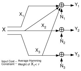
Figure 3: Equivalent Classical $3\mathchar 45\relax$user BC of Ex. 1.

Since Rxs $2$ and $3$ can be fed information only through $X_{2}$ and $X_{3}$ we are forced to choose $X_{2},X_{3}$ to be independent Ber$(\frac{1}{2})$ RVs throughout. Observe that Rx $1$ experiences an interference $X_{2}\oplus X_{3}$ which is now a Ber$(\frac{1}{2})$ RV. Furthermore, we recall that the average Hamming weight of $X_{1}$ is constrained to $\tau<\frac{1}{2}$. This has two imports. Firstly, the Tx cannot cancel off this interference that Rx $1$ experiences. Secondly, the maximum rate achievable for Rx $1$ is $C_{1}\mathrel{\ensurestackMath{\stackon[1pt]{=}{\scriptstyle\Delta}}}h_{b}(\tau*\epsilon)-h_{b}(\epsilon)$, where $*$ denotes binary convolution. Can the interference mitigation strategies available via unstructured coding achieve a rate $C_{1}$ for Rx $1$? In [10, Sec. III], we prove that no current known unstructured coding scheme can achieve a rate $C_{1}$ for Rx $1$. In the following, we explain the reasoning behind the deficiency of unstructured coding schemes.

The two interference mitigation strategies known are 1) Precoding for interference at the Tx, i.e. Marton’s binning and 2) decoding interference at the Rx partly or wholly via Han-Kobayashi’s message splitting. Since the unstructured coding schemes builds independent codes with independently picked codewords for every component of the signal, Rx $1$ is unable to decode $X_{2}\oplus X_{3}$ without decoding $X_{2},X_{3}$. A detailed proof in [10, Sec. III] establishes that unstructured coding schemes can enable the Rx $1$ decode only univariate functions $V_{2}=f_{2}(X_{2})$ and $V_{3}=f_{3}(X_{3})$ of $X_{2},X_{3}$ efficiently. If it has to decode a bi-variate function $g(X_{2},X_{3})$, the unstructured IID nature of the codes force the Rx to decode $X_{2}$ and $X_{3}$.

Can Rx $1$ decode $X_{2},X_{3}$ and achieve a rate $C_{1}$ for itself? Let us compare $\mathscr{C}_{1}$, defined as the capacity of $\underline{X}-Y_{1}$ link subject to $p_{X_{2}X_{3}}$ being uniform, with $C_{1}+C_{2}+C_{3}$. We have

$$\mathscr{C}_{1}\!=\!\sup_{p_{X_{1}}}I(Y_{1};\underline{X})\!=\!1\!-\!h_{b}(\epsilon)<\sum_{i=1}^{3}\!C_{i}\!=\!C_{1}\!+\!2\!-\!2h_{b}(\delta),\!\!\!$$ (2)

where the inequality in (2) follows by substituting $C_{1},C_{2},C_{3}$ and noting that $h_{b}(\delta)<\frac{1+h_{b}(\tau*\epsilon)}{2}$ for this example. This precludes Rx $1$ from decoding $X_{2},X_{3}$ and achieve a rate of $C_{1}$ for Rx $1$. Any unstructured coding scheme therefore leaves Rx $1$ with residual uncertainty of the interference $X_{2}\oplus X_{3}$. This forces the unstructured coding scheme to resort to the only other interference mitigating strategy - precoding for this residual uncertainty. In contrast to decoding interference, precoding in general entails a rate loss. In other words, the rate achievable by Rx $1$ if it can decode the entire interference and subtract it off is strictly larger that what it can achieve if some component of the interference is precoded for by the Tx.

Fact. 1.

Consider Ex. 1. The rate triple $(h_{b}(\tau*\epsilon)-h_{b}(\epsilon),1-h_{b}(\delta),1-h_{b}(\delta))$ is not achievable via any current known unstructured coding scheme.

We now present a simple linear coding scheme that can achieve the rate triple $(C_{1},C_{2},C_{3})$. In contrast to building independent codebooks for Rx $2$ and $3$, suppose we choose cosets $\lambda_{2},\lambda_{3}$ of a common linear code of rate $1-h_{b}(\delta)$ to communicate to both Rxs $2$ and $3$. Indeed, there exists cosets of a linear code that achieve capacity of a binary symmetric channel. Since the sum of two cosets is another coset of the same linear code, the interference patterns seen by Rx $1$ are constrained to another coset $\lambda_{2}\oplus\lambda_{3}$ of the same linear code of rate $1-h_{b}(\delta)$. Instead of attempting to decode the pair of Rx $2,3$’s codewords, suppose Rx $1$ decodes its the corresponding sum $\lambda_{2}\oplus\lambda_{3}$. Specifically, suppose Rx ${1}$ attempts to jointly decode it’s codeword and the sum of Rx $2$ and $3$’s codewords, the latter being present in $\lambda_{2}\oplus\lambda_{3}$, then it would be able to achieve a rate of $C_{1}$ for itself if

$$\mathscr{C}_{1}=1-h_{b}(\epsilon)>C_{1}+\max\{C_{2},C_{3}\}=C_{1}+1-h_{b}(\delta).\!\!\!$$ (3)

Substituting $C_{1}$, note that (3) is satisfied since $\tau*\epsilon<\delta$ for Ex. 1. Thus the coset code strategy permits Rx $1$ achieve a rate $C_{1}$ even while Rx $2$ and $3$ achieve rates $C_{2},C_{3}$ respectively.

Ex. 2.

Let $\underline{\mathcal{X}}=\mathcal{X}_{1}\times\mathcal{X}_{2}\times\mathcal{X}_{3}$ denote the input set with $\mathcal{X}_{j}=\{0,1\}$ for $j\in[3]$. For $b\in\{0,1\}$, let $\sigma_{b}^{1}(\eta)\mathrel{\ensurestackMath{\stackon[1pt]{=}{\scriptstyle\Delta}}}(1-\eta)\outerproduct{b}{b}+\eta\outerproduct{1-b}{1-b}$, and for $j=2,3$, let $\sigma_{0}^{j}=\outerproduct{0}{0}$ and $\sigma_{1}^{j}=\outerproduct{v_{\theta_{j}}}{v_{\theta_{j}}}$ where $\ket{v_{\theta_{j}}}=[\cos\theta_{j}~{}\sin\theta_{j}]^{T}$. For $\underline{x}=(x_{1},x_{2},x_{3})\in\underline{\mathcal{X}}$, let $\rho_{\underline{x}}=\sigma_{x_{1}\oplus x_{2}\oplus x_{3}}^{1}(\epsilon)\otimes\sigma_{x_{2}}^{2}\otimes\sigma_{x_{3}}^{3}$. The symbol $X_{1}$ is costed via a Hamming cost function i.e., the cost function $\kappa:\underline{\mathcal{X}}\rightarrow\{0,1\}$ is given by $\kappa(\underline{x})=x_{1}$. Let $0<\theta_{2}<\theta_{3}<\frac{\pi}{2}$, $\tilde{\delta}_{j}=\frac{1+\cos\theta_{j}}{2}$ and $\tau,\epsilon$ satisfy

$$h_{b}(\tau*\epsilon)+h_{b}(\tilde{\delta}_{2})+h_{b}(\tilde{\delta}_{3})\stackrel{{\scriptstyle(a)}}{{>}}1\stackrel{{\scriptstyle(b)}}{{>}}h_{b}(\tau*\epsilon)+h_{b}(\tilde{\delta}_{3}).$$ (4)

Comparing Exs. 1 and Ex. 2, note that the latter differs from the former only in components of Rxs $2$ and $3$. Moreover, it can be verified that for no choice of basis, is the collection $\rho_{\underline{x}}:\underline{x}\in\underline{\mathcal{X}}$ commuting. From [13, Ex.5.6], it is also clear that for $j=2,3$, the capacity of user $j$ is $C_{j}=h_{b}(\tilde{\delta}_{j})$ and is achieved by choosing $p_{X_{j}}$ uniform. Since $\frac{\pi}{2}>\theta_{3}>\theta_{2}>0$, we have $C_{3}>C_{2}$. If we subtract $h_{b}(\epsilon)$ to the two inequalities in (4), we obtain $C_{1}+C_{2}+C_{3}\stackrel{{\scriptstyle(a)}}{{>}}\mathscr{C}_{1}\stackrel{{\scriptstyle(b)}}{{>}}C_{1}+\max\{C_{2},C_{3}\}$, where $C_{1},\mathscr{C}_{1}$ are as defined for Ex. 1. From our discussion for Ex. 1 and inequality $(a)$, it is clear that unstructured codes cannot achieve the rate triple $(C_{1},C_{2},C_{3})$. If we can design capacity achieving linear codes $\lambda_{2},\lambda_{3}$ for Rxs $2,3$ respectively in such a way that $\lambda_{2}$ is a sub-coset of $\lambda_{3}$, then the interference patterns are contained within $\lambda_{2}\oplus\lambda_{3}$ which is now a coset of $\lambda_{3}$. Rx $1$ can therefore decode into this collection which is of rate atmost $C_{3}=h_{b}(\tilde{\delta}_{3})$. Inequality $(b)$ is analogous to the condition stated in (3) suggesting that coset codes can be achieve rate triple $(C_{1},C_{2},C_{3})$.

A reader may suspect whether gains obtained above via linear codes are only for ‘additive’ channels. Our study of [10, Ex. 2] and other settings [14] analytically prove that we can obtain gains for non-additive scenarios too. To harness such gains, it is necessary to design coding schemes that achieve rates for arbitrary distributions as proved in Thms. 1.

III-A Key Elements of a Generalized Coding Scheme

The codebooks of users $2$ and $3$ being cosets of a common linear code is central to the containment of the sum $X_{2}\oplus X_{3}$. In general users $2$ and $3$ may require codebooks of different rates. We therefore enforce that the smaller of the two codes be a sub-coset of the larger code. Secondly, in Ex. 1, users $2$ and $3$ could achieve capacity by choosing codewords that were uniformly distributed, i.e., typical with respect to the uniform distribution on $\{0,1\}$. Since all codewords of a random linear code are typical with respect to the uniform distribution, we could achieve capacity for users $2$ and $3$ by utilizing all codewords from the random linear code. In general, to achieve rates corresponding to non-uniform distributions, we have to enlarge the linear code beyond the desired rate and partition it into bins so that each bin contains codeword of the desired type. This leads us to a partitioned coset code (PCC) (Defn. 3) that is obtained by partitioning a coset code into bins that are individually unstructured.

IV Decoding Interference at a Single Rx

We provide a pedogogical description of our main results. In Sec. IV-A, we present a coding scheme involving three codebooks. Specifically, each user is equipped with one codebook. Rx $1$ decodes the sum of user $2$ and $3$’s codewords. In Sec. IV-F, we equip users $2$ and $3$ with two codebooks each, one of which is a private codebook whose codeword is decoded only by the corresponding Rx.

IV-A Decoding Sum of Private Codewords

We present our first inner bound to the capacity region of a $3\mathchar 45\relax$CQBC. In the sequel, we adopt the following notation. Suppose $S_{2},S_{3}$ and $B_{1}$ are real numbers, $U_{1},V_{2},V_{3}$ are random variables. For any $A\subseteq\{2,3\}$ and any $D\subseteq\{1\}$, let $S_{A}\mathrel{\ensurestackMath{\stackon[1pt]{=}{\scriptstyle\Delta}}}\sum_{a\in A}S_{a}$, $T_{A}\mathrel{\ensurestackMath{\stackon[1pt]{=}{\scriptstyle\Delta}}}\sum_{a\in A}T_{a}$, $B_{D}\mathrel{\ensurestackMath{\stackon[1pt]{=}{\scriptstyle\Delta}}}\sum_{d\in D}B_{d}$, $H(V_{A})\mathrel{\ensurestackMath{\stackon[1pt]{=}{\scriptstyle\Delta}}}H(V_{a}:a\in A)$, $H(V_{A},U_{D})=H(V_{a}:a\in A,U_{d}:d\in D)$ with the empty sum defined as $0$ throughout.

Theorem 1.

A rate-cost quadruple $(\underline{R},\tau)$ is achievable if there exists a finite set $\mathcal{U}_{1}$, a finite field $\mathcal{V}_{2}=\mathcal{V}_{3}=\mathcal{W}=\mathcal{F}_{q}$ of size $q$, real numbers $B_{1}\geq 0,S_{j}\geq 0,T_{j}=\frac{R_{j}}{\log q}\geq 0:j=2,3$ and a PMF $p_{XU_{1}V_{2}V_{3}}$ on $\mathcal{X}\times\mathcal{U}_{1}\times\mathcal{V}_{2}\times\mathcal{V}_{3}$ wrt which

$$(S_{A}-T_{A})\log q+B_{D} > \sum_{d\in D}\!H(U_{d})+\sum_{a\in A}\!H(V_{a})-H(V_{A},U_{D})+|A|\log q-\sum_{a\in A}\!H(V_{a})$$ (5)

$$\max\left\{S_{2}\log q+B_{D},S_{3}\log q+B_{D}\right\} > \log q-\min_{\theta\in\mathcal{F}_{q}\setminus\{0\}}H(V_{2}\oplus\theta V_{3}|U_{D}),$$ (6)

$$R_{1}+B_{1} < I(Y_{1},V_{2}\oplus_{q}V_{3};U_{1}),$$ (7)

$$\max\left\{S_{2}\log q,S_{3}\log q\right\} < I(Y_{1},U_{1};V_{2}\oplus_{q}V_{3})+\log q-H(V_{2}\oplus_{q}V_{3}),$$ (8)

$$\max\left\{R_{1}+B_{1}+S_{2}\log q,R_{1}+B_{1}+S_{3}\log q\right\} < I(Y_{1};V_{2}\oplus_{q}V_{3},U_{1})+I(U_{1};V_{2}\oplus_{q}V_{3})\log q-H(V_{2}\oplus_{q}V_{3})$$ (9)

$$S_{j}\log q < I(Y_{j};V_{j})+\log q-H(V_{j}):j=2,3,$$ (10)

for all $A\subseteq\{2,3\}$, $D\subseteq\{1\}$, $\sum_{x\in\mathcal{X}}p_{X}(x)\kappa(x)\leq\tau$, where all the above information quantities are computed wrt state,

$$\sigma^{\underline{Y}XU_{1}V_{2}V_{3}W}=\sum_{\begin{subarray}{c}x,u_{1},v_{2},v_{3},w\end{subarray}}p_{XU_{1}V_{2}V_{3}W}(x,u_{1},v_{1},v_{2},w)\rho_{x}\otimes\outerproduct{x~{}u_{1}~{}v_{2}~{}v_{3}~{}w}{x~{}u_{1}~{}v_{2}~{}v_{3}~{}w}\mbox{ with}$$ (11)

$$p_{XU_{1}V_{2}V_{3}W}\left({x,u_{1},v_{2},v_{3},w}\right)=p_{XU_{1}V_{2}V_{3}}\left({x,u_{1},v_{2},v_{3}}\right)\mathds{1}_{\{\begin{subarray}{c}w=v_{2}\oplus_{q}v_{3}\end{subarray}\}}$$

$\forall(x,u_{1},v_{2},v_{3},w)\in\mathcal{X}\times\mathcal{U}_{1}\times\mathcal{V}_{2}\times\mathcal{V}_{3}\times\mathcal{W}$.

Prop. 1.

Consider Ex. 2. The rate triple $(h_{b}(\tau*\epsilon)-h_{b}(\epsilon),h_{b}(\tilde{\delta_{2}}),h_{b}(\tilde{\delta_{3}}))$ is achievable if (4)$(b)$ holds. This triple is not achievable via IID codes if (4)$(a)$ holds.

In order to prove the first statement of Prop. 1, we identify a choice of parameters in statement of Thm. 1 and verify the bounds. Towards that end, consider $\mathcal{U}_{1}=\mathcal{X}_{1},\mathcal{V}_{j}=\mathcal{X}_{j}$, $X_{1}=U_{1}$, $X_{j}=V_{j}$ for $j=2,3$, $p_{X_{1}X_{2}X_{3}}(x_{1},x_{2},x_{3})=\frac{1-\tau}{4}$ if $x_{1}=0$ $p_{X_{1}X_{2}X_{3}}(x_{1},x_{2},x_{3})=\frac{\tau}{4}$ if $x_{1}=1$, $S_{j}=T_{j}=h_{b}(\tilde{\delta_{3}})$, $R_{1}=h_{b}(\tau*\epsilon)-h_{b}(\epsilon)$, $B_{1}=0$. We now verify the bounds in (5) - (10). Since $X_{1}=U_{1},X_{2}=v_{2}$ and $X_{3}=V_{3}$ are independent and moreover $H(V_{2})=H(V_{3})=\log 2$ and $q=2$, it can be verified that the lower bounds in (5) and (6) are $0$. This implies our choice $B_{1}=0$ and $S_{j}=T_{j}$ do not violate these bounds. With the choice for $p_{X_{1}}=p_{U_{1}}$, it can be verified that the upper bound on (i) $R_{1}$ in (7) is $h_{b}(\tau*\epsilon)-h_{b}(\epsilon)$, (ii) $S_{3}\log q$ in (8) is $1-h_{b}(\epsilon)$, (iii) $R_{1}+S_{3}\log q$ in (9) is $1-h_{b}(\epsilon)$ and (iv) $S_{j}\log q$ in (10) is $h_{b}(\tilde{\delta_{j}})$. Since (4)$(b)$ holds, all of these bounds are satisfied. The proof of the second statement is based on our proof of Fact 1 that is provided in [10, Sec. III]. From the similarity of the examples, this can be verified.

Remark 2.

The inner bound in Thm. 1 is characterized via additional code parameters $B_{1},S_{2},S_{3}$. To characterize an inner bound in terms of only $R_{1},R_{2},R_{3}$, we perform a variable elimination. Instead of using the Fourier Motzkin technique, we leverage the technique proposed in [15] to perform variable elimination. In Corollary 1, we state the resulting inner bound obtained by eliminating variables $B_{1},S_{2}$ and $S_{3}$ in Thm. 1.

Proof.

We begin by outlining our techniques and identifying the new elements. The main novelty is in 1) the code structure (Sec. IV-B) that involves jointly designed PCCs built over $\mathcal{F}_{q}$ for users $2$, $3$, and 2) the decoding rule (Sec. IV-D) wherein Rx $1$ decodes the sum of users $2$ and $3$’s codewords to facilitate interference peeling. We adopt Marton’s encoding (Sec. IV-C) of identifying a jointly typical triple, point-to-point decoder POVMs for Rxs $2,3$ and the joint decoder proposed in [16] for Rx $1$. Since the random codewords of users $2,3$ are uniformly distributed and statistically correlated, we are forced to go beyond a ‘standard information theory proof’ and carefully craft our analysis steps. We adapt the steps in [16, Proof of Thm. 2] to analyze Rx $1$’s error and those in [4, Proof of Thm. 2] to analyze Rx $2,3$’s error. Specifically, a new element in our analysis is the use of ‘list threshold’ event ($\mathcal{E}_{\underline{m}}$) that enables us recover a binning exponent (Rem. 3).

IV-B Code Structure

We design a coding scheme with parameters $R_{1},B_{1},S_{2},T_{2},S_{3},T_{3}$ that communicates at rates $R_{1}$ to Rx 1 and $R_{j}=T_{j}\log q$ to Rxs $j=2,3$ respectively. Let $\mathcal{U}_{1}$ be a finite set and $\mathcal{V}_{2}=\mathcal{V}_{3}=\mathcal{F}_{q}$ be the finite field of cardinality $q$. Rx $1$’s message is communicated via codebook $\mathcal{C}_{1}=(u_{1}^{n}(m_{1},b_{1}):m_{1}\in[\mathcal{M}_{1}]=[2^{nR_{1}}],b_{1}\in[2^{nB_{1}}])$ built over $\mathcal{U}_{1}$. As discussed in Sec. III-A, Rx $2$ and $3$’s messages are communicated via PCCs that are characterized below.

Defn. 3.

A partitioned coset code (PCC) built over a finite field $\mathcal{V}=\mathcal{F}_{q}$ comprises of (i) a generator matrix $g\in\mathcal{V}^{s\times n}$, (ii) a shift vector $d^{n}\in\mathcal{V}^{n}$ and (iii) a binning map $\iota:\mathcal{V}^{s}\rightarrow\mathcal{V}^{t}$. We let $v^{n}(a^{s})\mathrel{\ensurestackMath{\stackon[1pt]{=}{\scriptstyle\Delta}}}a^{s}g\oplus_{q}d^{n}:a^{s}\in\mathcal{V}^{s}$ denote its codewords, $c(m^{t})=\{a^{s}\in\mathcal{V}^{s}:\iota(a^{s})=m^{t}\}$ denote the bin corresponding to message $m^{t}$, $S=\frac{s}{n}$ and $T=\frac{t}{n}$. When clear from context, we ignore superscripts $s$ in $a^{s}$ and $t$ in $m^{t}$. We refer to this as PCC $(n,S,T,g,d^{n},\iota)$ or PCC $(n,S,T,g,d^{n},c)$.

For $j=2,3$, Rx $j$’s message is communicated via PCC $\lambda_{j}$. In Sec. III-A, we noted that the smaller of these codes must be a sub-coset of the larger code. Without loss of generality assume $\lambda_{3}$ is larger than $\lambda_{2}$, we let $\lambda_{j}$ be the PCC $(n,S_{j},T_{j},g_{j},d_{j}^{n},\iota_{j})$ where $g_{3}=\left[g_{2}^{T}~{}g_{3/2}^{T}\right]^{T}$, $g_{2}\in\mathcal{V}^{s_{2}\times n}$ and $g_{3/2}\in\mathcal{V}^{(s_{3}-s_{2})\times n}$. This guarantees that the collection of vectors obtained by adding all possible pairs of codewords from $\lambda_{2}$ and $\lambda_{3}$ is the collection $\lambda_{\mbox{{\tiny$\oplus$}}}\mathrel{\ensurestackMath{\stackon[1pt]{=}{\scriptstyle\Delta}}}(w^{n}(a_{\mbox{{\tiny$\oplus$}}})\mathrel{\ensurestackMath{\stackon[1pt]{=}{\scriptstyle\Delta}}}a_{\mbox{{\tiny$\oplus$}}}g_{3}\oplus_{q}d_{\mbox{{\tiny$\oplus$}}}^{n}:a_{\mbox{{\tiny$\oplus$}}}\in\mathcal{V}^{s_{3}})$ where $d_{\mbox{{\tiny$\oplus$}}}\mathrel{\ensurestackMath{\stackon[1pt]{=}{\scriptstyle\Delta}}}d_{2}^{n}\oplus_{q}d_{3}^{n}$. For $j=2,3$ let $\mathcal{M}_{j}=q^{t_{j}}$ and $[\mathcal{M}_{j}]\mathrel{\ensurestackMath{\stackon[1pt]{=}{\scriptstyle\Delta}}}[q^{t_{j}}]$ denote Rx $j$ message index set.

IV-C Encoding

The triple $(u_{1}^{n}(m_{1},b_{1}):b_{1}\in[2^{nB_{1}}]),c_{2}(m_{2}),c_{3}(m_{3})$ of bins correspond to the available choice of codewords that the encoder can use to communicate the message triple $\underline{m}\mathrel{\ensurestackMath{\stackon[1pt]{=}{\scriptstyle\Delta}}}(m_{1},m_{2},m_{3})\in[\underline{\mathcal{M}}]$. Let

$$\mathcal{L}(\underline{m})\mathrel{\ensurestackMath{\stackon[1pt]{=}{\scriptstyle\Delta}}}\left\{\!\!\!\begin{array}[]{c}(b_{1},a_{2},a_{3}):b_{1}\in[2^{nB_{1}}],a_{j}\in c_{j}(m_{j}):j=2,3\\ \ni(u_{1}(m_{1},b_{1}),v_{2}(a_{2}),v_{3}(a_{3}))\in T_{\eta}(p_{U_{1}V_{2}V_{3}}),\end{array}\!\!\!\right\}$$ (14)

be a list of typical triples among this choice and $\alpha(\underline{m})\mathrel{\ensurestackMath{\stackon[1pt]{=}{\scriptstyle\Delta}}}|\mathcal{L}(\underline{m})|$. Let $(b_{1}(\underline{m}),a_{2}(\underline{m}),a_{3}(\underline{m}))$ be a triple chosen from $\mathcal{L}(\underline{m})$ if $\alpha(\underline{m})\geq 1$. Otherwise, set $(b_{1}(\underline{m}),a_{2}(\underline{m}),a_{3}(\underline{m}))=(1,0^{s_{2}},0^{s_{3}})$. A ‘fusion map’ $f:\mathcal{U}_{1}^{n}\times\mathcal{V}_{2}^{n}\times\mathcal{V}_{3}^{n}\rightarrow\mathcal{X}^{n}$ is used to map $(u_{1}^{n}(m_{1},b_{1}(\underline{m})),v_{2}(a_{2}(\underline{m})),v_{3}(a_{3}(\underline{m})))$ into an input sequence henceforth denoted as $x^{n}(\underline{m})\mathrel{\ensurestackMath{\stackon[1pt]{=}{\scriptstyle\Delta}}}(x(\underline{m})_{t}:t\in[n])$. To communicate a message triple $\underline{m}$, the encoder prepares the state $\rho_{\underline{m}}\mathrel{\ensurestackMath{\stackon[1pt]{=}{\scriptstyle\Delta}}}\otimes_{t=1}^{n}\rho_{x(\underline{m})_{t}}$.

IV-D Decoding POVMs

In addition to $m_{1}$, Rx $1$ aims to decode the sum $v_{2}(a_{2}(\underline{m}))\oplus v_{3}(a_{3}(\underline{m}))$ of the codewords chosen by the Tx. To reference this sum succinctly, henceforth we let $a_{\oplus}(\underline{m})=a_{2}(\underline{m})0^{s_{3}-s_{2}}\oplus_{q}a_{3}(\underline{m})$. Recollecting code $\lambda_{\mbox{{\tiny$\oplus$}}}$, it can be verified that the sum $v_{2}(a_{2}(\underline{m}))\oplus v_{3}(a_{3}(\underline{m}))=w^{n}(a_{\oplus}(\underline{m}))$. Rx $1$ employs the decoding POVM [16, Proof of Thm. 2]

$$\theta_{m_{1},b_{1}}^{a_{\mbox{{\tiny$\oplus$}}}}\!\!\mathrel{\ensurestackMath{\stackon[1pt]{=}{\scriptstyle\Delta}}}\!\!\left(\sum_{\hat{m}_{1},\hat{b}_{1},\hat{a}_{\mbox{{\tiny$\oplus$}}}}\!\!\!\!\lambda_{\hat{m}_{1},\hat{b}_{1}}^{\hat{a}_{\mbox{{\tiny$\oplus$}}}}\!\!\right)^{\!\!-\frac{1}{2}}\!\!\!\!\!\lambda_{m_{1},b_{1}}^{a_{\mbox{{\tiny$\oplus$}}}}\!\!\left(\sum_{\hat{m}_{1},\hat{b}_{1},\hat{a}_{\mbox{{\tiny$\oplus$}}}}\!\!\!\lambda_{\hat{m}_{1},\hat{b}_{1}}^{\hat{a}_{\mbox{{\tiny$\oplus$}}}}\!\right)^{\!\!-\frac{1}{2}}$$

where $\lambda_{m_{1},b_{1}}^{a_{\mbox{{\tiny$\oplus$}}}}\mathrel{\ensurestackMath{\stackon[1pt]{=}{\scriptstyle\Delta}}}\pi^{Y_{1}}\pi_{m_{1},b_{1}}\pi_{m_{1},b_{1}}^{a_{\mbox{{\tiny$\oplus$}}}}\pi_{m_{1},b_{1}}\pi^{Y_{1}}$,

$$\pi_{m_{1},b_{1}}\mathrel{\ensurestackMath{\stackon[1pt]{=}{\scriptstyle\Delta}}}\pi_{u_{1}^{n}(m_{1},b_{1})}^{Y_{1}},~{}~{}~{}\pi^{a_{\mbox{{\tiny$\oplus$}}}}_{m_{1},b_{1}}\mathrel{\ensurestackMath{\stackon[1pt]{=}{\scriptstyle\Delta}}}\pi^{Y_{1}}_{u_{1}^{n}(m_{1},b_{1}),w^{n}(a_{\mbox{{\tiny$\oplus$}}})}.$$ (15)

are the C-Typ-Projs. with respect to states to $\rho^{Y_{1}}_{u_{1}}=\tr_{Y_{2}Y_{3}}(\sum_{x}p_{X|U_{1}}(x|u_{1})\rho_{x}^{\underline{Y}})$ and

$$\rho_{u_{1}w}^{Y_{1}}\mathrel{\ensurestackMath{\stackon[1pt]{=}{\scriptstyle\Delta}}}\tr_{Y_{2}Y_{3}}\left(\sum_{x}p_{X|U_{1}W}(x|u_{1},w)\rho_{x}^{\underline{Y}}\right)$$

respectively.

Rxs $2$ and $3$ decode only their messages. Rx $j$ employs the POVM $\{\theta_{m_{j}}=\displaystyle\!\!\!\!\!\!\!\sum_{a_{j}\in c_{j}(m_{j})}\!\!\!\!\!\!\!\!\theta_{a_{j}}:m_{j}\in[\mathcal{M}_{j}]\}$ where

$$\theta_{a_{j}}\!\mathrel{\ensurestackMath{\stackon[1pt]{=}{\scriptstyle\Delta}}}\!\left(\!\!\sum_{\hat{a}_{j}}\pi^{Y_{j}}\pi_{\hat{a}_{j}}\pi^{Y_{j}}\!\!\right)^{\!\!\!-\frac{1}{2}}\!\!\!\pi^{Y_{j}}\pi_{a_{j}}\pi^{Y_{j}}\!\!\left(\sum_{\hat{a}_{j}}\pi^{Y_{j}}\pi_{\hat{a}_{j}}\pi^{Y_{j}}\right)^{\!\!\!-\frac{1}{2}}\!\!\!\!\!\!,$$

$\pi^{Y_{2}},\pi^{Y_{3}}$ are the U-Typ-Proj of $\rho^{Y_{2}},\rho^{Y_{3}}$ respectively, and for $j=2,3$, $\pi_{a_{j}}\mathrel{\ensurestackMath{\stackon[1pt]{=}{\scriptstyle\Delta}}}\pi_{v_{j}^{n}(a_{j})}$ is the C-Typ-Proj wrt state $\rho_{v_{j}}^{Y_{j}}\mathrel{\ensurestackMath{\stackon[1pt]{=}{\scriptstyle\Delta}}}\tr_{Y_{1}Y_{\text{\sout{$j$}}}}(\sum_{x}p_{X|V_{j}}(x|v_{j})\rho_{x}^{\underline{Y}})$.

IV-E Probability of Error Analysis

We first state the distribution of the random code. Codewords of $\mathcal{C}_{1}$ are picked IID $\prod p_{U_{1}}$. The generator matrix $G_{3}$, shifts $D_{2}^{n},D_{3}^{n}$, bin indices $(\iota_{j}(a_{j}):a_{j}\in\mathcal{F}_{q}^{s_{j}}):j=2,3$ are all picked mutually independently and uniforSubSec:DecSumOfPublicCdwrdsmly from their respective ranges. If $\alpha(\underline{m})\geq 1$, $(B_{1}(\underline{m}),A_{2}(\underline{m}),A_{3}(\underline{m}))$ is picked uniformly from $\mathcal{L}(\underline{m})$. Otherwise, $(B_{1}(\underline{m}),A_{2}(\underline{m}),A_{3}(\underline{m}))\mathrel{\ensurestackMath{\stackon[1pt]{=}{\scriptstyle\Delta}}}(1,0^{s_{2}},0^{s_{3}})$. All of the above objects are also mutually independent. We emphasize that $(B_{1}(\underline{m}),A_{2}(\underline{m}),A_{3}(\underline{m}))$ is conditionally independent of $\mathcal{C}_{1},G_{3},D_{2}^{n},D_{3}^{n}$, $(\iota_{j}(a_{j}):a_{j}\in\mathcal{F}_{q}^{s_{j}}):j=2,3$ given the event $\{\alpha(\underline{m})\geq 1\}$, a fact (Note 1) we shall use at a later point in our analysis. Finally, $X^{n}(\underline{m})$ is picked according to $p_{X|U_{1}V_{2}V_{3}}^{n}(\cdot|V_{1}^{n}(m_{1},b_{1}(\underline{m})),V_{2}(A_{2}(\underline{m})),V_{3}(A_{3}(\underline{m})))$.

The average probability of error is

$$P(\mbox{Err})\!=\!\frac{1}{|\underline{\mathcal{M}}|}\!\sum_{\underline{m}\in[\underline{\mathcal{M}}]}\!\!\!{\tr\!\left\{\!\left(\!I_{{\underline{Y}}}^{\otimes n}\!\!-\!\theta^{a_{\mbox{{\tiny$\oplus$}}}(\underline{m})}_{m_{1},b_{1}}\otimes\theta_{m_{2}}\otimes\theta_{m_{3}}\!\right)\!\rho_{\underline{m}}\right\}\!}.$$ (16)

Henceforth, we analyze a generic term $\xi_{\underline{m}}$ in the sum (16). Define a ‘list threshold’ event $\mathcal{E}_{\underline{m}}\mathrel{\ensurestackMath{\stackon[1pt]{=}{\scriptstyle\Delta}}}\{\alpha(\underline{m})\geq 2^{n(\tau-\eta)\}}$ where

$$\tau\mathrel{\ensurestackMath{\stackon[1pt]{=}{\scriptstyle\Delta}}}B_{1}\!+\!\sum_{j=2}^{3}\!(S_{j}-T_{j})\log q\!-\!2\log q\!+\!H(V_{2},V_{3}|U_{1}\!),$$ (17)

is the exponent of the expected number of jointly typical triples in any triple of bins and $\mathds{1}_{\mathcal{E}_{\underline{m}}}$ be its indicator. Firstly, note that every term $\xi_{\underline{m}}$ in the above sum is at most $1$. Hence $\xi_{\underline{m}}\mathds{1}_{\mathcal{E}^{c}_{\underline{m}}}\leq\mathds{1}_{\mathcal{E}^{c}_{\underline{m}}}$. Next, note that the operator inequalities $0\leq\theta^{a_{\mbox{{\tiny$\oplus$}}}(\underline{m})}_{m_{1},b_{1}}\leq I_{Y_{1}}$ and $0\leq\theta_{m_{j}}\leq I_{Y_{j}}$ hold. We therefore have

$$\xi_{\underline{m}}\!\mathrel{\ensurestackMath{\stackon[1pt]{=}{\scriptstyle\Delta}}}\!\tr\!\left\{\!\!\left(\!I_{{\underline{Y}}}^{\otimes n}-\theta^{a_{\mbox{{\tiny$\oplus$}}}(\underline{m})}_{m_{1},b_{1}}\!\!\otimes\!\theta_{m_{2}}\!\!\otimes\!\theta_{m_{3}}\!\!\right)\!\rho_{\underline{m}}\!\right\}\!\leq T_{0}+T_{1}+T_{2}+T_{3}\!\!\!\!\!\!\!\!\!\!\!\!$$

$$\mbox{where }T_{0}=\mathds{1}_{\mathcal{E}_{\underline{m}}^{c}},~{}T_{1}\mathrel{\ensurestackMath{\stackon[1pt]{=}{\scriptstyle\Delta}}}\tr_{Y_{1}}\!\!\left\{\!\left(I_{Y_{1}}-\theta_{m_{1},b_{1}}^{a_{\mbox{{\tiny$\oplus$}}}(\underline{m})}\right)\!\rho_{\underline{m}}^{Y_{1}}\!\right\}\mathds{1}_{\mathcal{E}_{\underline{m}}},$$ (18)

$$T_{j}\mathrel{\ensurestackMath{\stackon[1pt]{=}{\scriptstyle\Delta}}}\tr_{Y_{j}}\!\!\left\{\left(I_{Y_{j}}-\theta_{m_{j}}\right)\!\rho_{\underline{m}}^{Y_{j}}\!\right\}\mathds{1}_{\mathcal{E}_{\underline{m}}}\mbox{ for }j=2,3,$$ (19)

where $\xi_{\underline{m}}\mathds{1}_{\mathcal{E}_{\underline{m}}}\leq T_{1}+T_{2}+T_{3}$ is true because whenever operators $A_{i}$ satisfy $0\leq A_{i}\leq I_{Y_{i}}$ for $i\in[3]$, we have $I_{Y_{1}}\!\otimes\!I_{Y_{2}}\!\otimes\!I_{Y_{3}}\!-\!A_{1}\!\otimes\!A_{2}\!\otimes\!A_{3}\!\leq\!I_{Y_{1}}\!\otimes\!I_{Y_{2}}\!\otimes\!(I_{Y_{3}}\!-\!A_{3})\!+\!I_{Y_{1}}\!\otimes\!(I_{Y_{2}}\!-\!A_{2})\!\otimes\!I_{Y_{3}}\!+\!(I_{Y_{1}}\!-\!A_{1})\!\otimes\!I_{Y_{2}}\!\otimes\!I_{Y_{3}}$. This is analogous to a ‘union bound’ [2, Eqn. $78$] in classical probability. The rest of our proof analyzes each of $T_{0},T_{1},T_{2}$ and $T_{3}$.

Remark 3.

We have tagged along $\mathds{1}_{\mathcal{E}_{\underline{m}}}$ to suppress a binning exponent in our pre-variable-elimination bounds. While this does not enlarge the rate region, it enables our variable elimination to yield a compact description of the inner bound. Specifically, if we had not tagged along this event and not suppressed the binning exponent, then a variable elimination performed on the characterization in Thm. 1 would yield far more inequalities post variable elimination as compared to that provided in Corollary 1.

Analysis of $T_{0}$ : Since $T_{0}$ involves only classical probabilities, its analysis is identical to that in [10, App. 1] and we therefore refer the reader to [10, App. 1] for a proof of Prop. 2.

Prop. 2.

For any $\eta>0$, there exists $N_{\eta}\in\mathbb{N}$ such that for all $n\geq N_{\eta}$, we have $\mathbb{E}\{T_{0}\}\leq\exp\{-n\eta\}$ if the bounds (5), (6) in the Thm. 1 statement holds for all $A\subseteq\{2,3\}$ and every $D\subseteq\{1\}$ with the empty sum being defined as $0$.

To comprehend the above bounds, note that the first $3$ terms on the RHS form the usual lower bound in classical covering. The extra $|A|\log q-\sum_{a\in A}H(V_{a})$ is the penalty in binning rate we pay since the codewords of the linear code are uniformly distributed. Indeed, this is the divergence $D(p_{V_{A}}||\mbox{Unif}^{|A|})$ between the desired distribution and the uniform on $\mathcal{F}_{q}^{|A|}$.

Analysis of $T_{1}$ : Let $\pi_{a_{\mbox{{\tiny$\oplus$}}}(\underline{m})}=\pi_{w^{n}(a_{\mbox{{\tiny$\oplus$}}}(\underline{m}))}$ be the conditional typical projector with respect to the state $\rho_{w}^{Y_{1}}\mathrel{\ensurestackMath{\stackon[1pt]{=}{\scriptstyle\Delta}}}\tr_{Y_{2}Y_{3}}\left(\sum_{x}p_{X|W}(x|w)\rho_{x}^{\underline{Y}}\right)$. Since we have fixed an arbitrary $\underline{m}$, we let $a_{\mbox{{\tiny$\oplus$}}}=a_{\mbox{{\tiny$\oplus$}}}(\underline{m})$ and $\pi_{a_{\mbox{{\tiny$\oplus$}}}}\mathrel{\ensurestackMath{\stackon[1pt]{=}{\scriptstyle\Delta}}}\pi_{a_{\mbox{{\tiny$\oplus$}}}(\underline{m})}$in the sequel. We adapt [16, Proof of Thm. 2] to derive our upper bound on $T_{1}$. From the definition of $T_{1}$ in (18) and the fact that $\tr(\lambda\rho)\leq\tr(\lambda\sigma)+\norm{\rho-\sigma}_{1}$ for $0\leq\rho,\sigma,\lambda\leq I$, we have

$$T_{1}\leq\tr_{Y_{1}}\!\!\left\{\!\left(I_{Y_{1}}-\theta_{m_{1},b_{1}}^{a_{\mbox{{\tiny$\oplus$}}}}\right)\!\pi_{a_{\mbox{{\tiny$\oplus$}}}}\rho_{\underline{m}}^{Y_{1}}\pi_{a_{\mbox{{\tiny$\oplus$}}}}\!\right\}\mathds{1}_{\mathcal{E}_{\underline{m}}}+T_{10}$$ (20)

where $T_{10}=\norm{\pi_{a_{\mbox{{\tiny$\oplus$}}}}\rho_{\underline{m}}^{Y_{1}}\pi_{a_{\mbox{{\tiny$\oplus$}}}}-\rho_{\underline{m}}^{Y_{1}}}_{1}\mathds{1}_{\mathcal{E}_{\underline{m}}}$. Since $\alpha(\underline{m})\geq 1$, the chosen triple of codewords is jointly typical and by pinching and the gentle operator lemma, we have $\mathbb{E}\{T_{10}\}\leq\exp\{-n\eta\}$ for sufficiently large $n$. Denoting the first term in (20) as $\overline{T}_{11}$ and applying the Hayashi-Nagaoka inequality [17] on $\overline{T}_{11}$, we have $\overline{T}_{11}\leq 2(I-T_{11})\mathds{1}_{\mathcal{E}_{\underline{m}}}+4(T_{12}+T_{13}+T_{14})\mathds{1}_{\mathcal{E}_{\underline{m}}}$, where

$$T_{11}\mathrel{\ensurestackMath{\stackon[1pt]{=}{\scriptstyle\Delta}}}\tr\!\left(\!\lambda_{m_{1},b_{1}}^{a_{\mbox{{\tiny$\oplus$}}}}\pi_{a_{\mbox{{\tiny$\oplus$}}}}\rho_{\underline{m}}^{Y_{1}}\pi_{a_{\mbox{{\tiny$\oplus$}}}}\!\right)\!,T_{12}\!\mathrel{\ensurestackMath{\stackon[1pt]{=}{\scriptstyle\Delta}}}\!\!\!\!\!\!\sum_{\begin{subarray}{c}(\hat{m}_{1},\hat{b}_{1})\neq\\ (m_{1},b_{1})\end{subarray}}\!\!\!\!\!\!\!\tr(\!\lambda_{\hat{m}_{1},\hat{b}_{1}}^{a_{\mbox{{\tiny$\oplus$}}}}\!\!\pi_{a_{\mbox{{\tiny$\oplus$}}}}\rho_{\underline{m}}^{Y_{1}}\pi_{a_{\mbox{{\tiny$\oplus$}}}}\!\!)$$

$$T_{13}\!\mathrel{\ensurestackMath{\stackon[1pt]{=}{\scriptstyle\Delta}}}\!\!\!\!\sum_{\begin{subarray}{c}\hat{a}_{\mbox{{\tiny$\oplus$}}}\neq a_{\mbox{{\tiny$\oplus$}}}\end{subarray}}\!\!\!\!\!\tr(\!\lambda_{m_{1},b_{1}}^{\hat{a}_{\mbox{{\tiny$\oplus$}}}}\!\!\pi_{a_{\mbox{{\tiny$\oplus$}}}}\rho_{\underline{m}}^{Y_{1}}\pi_{a_{\mbox{{\tiny$\oplus$}}}}\!\!),T_{14}\!\mathrel{\ensurestackMath{\stackon[1pt]{=}{\scriptstyle\Delta}}}\!\!\!\!\!\!\!\!\!\!\!\!\!\!\sum_{\begin{subarray}{c}\hat{a}_{\mbox{{\tiny$\oplus$}}}\neq a_{\mbox{{\tiny$\oplus$}}}\\ (\hat{m}_{1},\hat{b}_{1})\neq(m_{1},b_{1})\end{subarray}}\!\!\!\!\!\!\!\!\!\!\!\!\!\!\!\tr(\!\lambda_{\hat{m}_{1},\hat{b}_{1}}^{\hat{a}_{\mbox{{\tiny$\oplus$}}}}\!\!\pi_{a_{\mbox{{\tiny$\oplus$}}}}\rho_{\underline{m}}^{Y_{1}}\pi_{a_{\mbox{{\tiny$\oplus$}}}}\!\!)$$

Analysis of $T_{11}$ is straightforward involving repeated use of the gentle operator lemma. See [11] for detailed steps.

Analysis of $T_{12},T_{13},T_{14}$ : We pull forward our new steps that enable us analyze $T_{12},T_{13},T_{14}$ and illustrate them below in a unified manner. Abbreviating $\underline{v}^{n}=(v_{2}^{n},v_{3}^{n})$, $\underline{V}=(V_{2},V_{3})$, recalling $a_{\mbox{{\tiny$\oplus$}}}=a_{\mbox{{\tiny$\oplus$}}}(\underline{m})$ and with a slight abuse of notation, let

$$\mathcal{F}_{1}\!\!\mathrel{\ensurestackMath{\stackon[1pt]{=}{\scriptstyle\Delta}}}\!\!\left\{\!\!\!\!\begin{array}[]{c}V_{j}^{n}(a_{j})=v_{j}^{n},\iota_{j}(a_{j})=m_{j}\!:\!j\!=\!2,3,U_{1}(m_{1},b_{1})=u_{1}^{n},W^{n}(a_{\mbox{{\tiny$\oplus$}}})=w^{n}\end{array}\!\!\!\!\right\}\!,\mathcal{B}\!\mathrel{\ensurestackMath{\stackon[1pt]{=}{\scriptstyle\Delta}}}\!{\left\{\!{(u_{1}^{n},\underline{v}^{n},w^{n})\in T_{\eta}\!(p_{U_{1}\underline{V}W}\!)}\!\right\}}$$ (22)

$$\mathcal{F}_{2}\!\mathrel{\ensurestackMath{\stackon[1pt]{=}{\scriptstyle\Delta}}}\!\left\{\!\!\!\!\begin{array}[]{c}B_{1}(\underline{m})=b_{1},A_{j}(\underline{m})=a_{j}\end{array}\!\!\!:\!\!\begin{array}[]{c}j=2,3\end{array}\!\!\!\right\},~{}\mathcal{G}_{12}=\left\{\!\!\!\!\begin{array}[]{c}U_{1}^{n}(\hat{m}_{1},\hat{b}_{1})=\hat{u}_{1}^{n},(\hat{m}_{1},\hat{b}_{1})\neq(m_{1},b_{1})\end{array}\!\!\!\right\}$$ (26)

$$\mathcal{F}_{3}\!\mathrel{\ensurestackMath{\stackon[1pt]{=}{\scriptstyle\Delta}}}\!\{X^{n}(\underline{m})=x^{n}\!\},\mathcal{G}_{13}\mathrel{\ensurestackMath{\stackon[1pt]{=}{\scriptstyle\Delta}}}\left\{\!\!\!\!\begin{array}[]{c}W^{n}(\hat{a}_{\mbox{{\tiny$\oplus$}}})=\hat{w}^{n},\hat{a}_{\mbox{{\tiny$\oplus$}}}\neq a_{\mbox{{\tiny$\oplus$}}}\end{array}\!\!\!\!\right\},\mathcal{G}_{14}\mathrel{\ensurestackMath{\stackon[1pt]{=}{\scriptstyle\Delta}}}\mathcal{G}_{12}\cap\mathcal{G}_{13},\mathcal{A}\mathrel{\ensurestackMath{\stackon[1pt]{=}{\scriptstyle\Delta}}}\left\{\!\!\!\!\begin{array}[]{c}(\hat{u}_{1}^{n},w^{n})\in T_{\eta}(p_{U_{1}W})\end{array}\!\!\!\!\right\},$$ (29)

where the event $\mathcal{F}_{1}\cap\mathcal{F}_{2}\cap\mathcal{F}_{3}$ specifies the realization for the chosen codewords and $\mathcal{G}_{12},\mathcal{G}_{13},\mathcal{G}_{14}$ specify the realization of an incorrect codeword in regards to $T_{12},T_{13},T_{14}$ respectively. We let $\lambda_{u_{1}^{n},w^{n}}\mathrel{\ensurestackMath{\stackon[1pt]{=}{\scriptstyle\Delta}}}\pi^{Y_{1}}\pi_{u_{1}^{n}}\pi_{u_{1}^{n}w^{n}}\pi_{u_{1}^{n}}\pi^{Y_{1}}$ as in (15), $\mathcal{E}_{1k}\mathrel{\ensurestackMath{\stackon[1pt]{=}{\scriptstyle\Delta}}}\mathcal{F}_{1}\cap\mathcal{G}_{1k}\cap\mathcal{E}_{\underline{m}}\cap\mathcal{F}_{2}\cap\mathcal{F}_{3}\cap\mathcal{A}\cap\mathcal{B}$ for $k=2,3,4$ and note that

$$\mathbb{E}\{T_{12}\mathds{1}_{\mathcal{E}_{\underline{m}}}\}=\!\!\!\!\!\!\sum_{\begin{subarray}{c}b_{1},a_{2},a_{3}\\ u_{1}^{n},v_{2}^{n},v_{3}^{n}\end{subarray}}\sum_{\begin{subarray}{c}w^{n},x^{n}\\ \hat{m}_{1},\hat{b}_{1},\hat{u}_{1}^{n}\end{subarray}}\!\!\!\!\!\!\tr(\lambda_{\hat{u}_{1}^{n},w^{n}}\!\pi_{w^{n}}\rho_{x^{n}}\pi_{w^{n}}\!)P(\mathcal{E}_{12})$$ (30)

$$\mathbb{E}\{T_{13}\mathds{1}_{\mathcal{E}_{\underline{m}}}\}=\!\!\!\!\!\!\!\sum_{\begin{subarray}{c}b_{1},a_{2},a_{3}\\ u_{1}^{n},v_{2}^{n},v_{3}^{n}\end{subarray}}\sum_{\begin{subarray}{c}w^{n},x^{n}\\ \hat{a}_{\mbox{{\tiny$\oplus$}}},\hat{w}^{n}\end{subarray}}\!\!\!\tr(\lambda_{u_{1}^{n},\hat{w}^{n}}\pi_{w^{n}}\rho_{x^{n}}\pi_{w^{n}}\!)P(\mathcal{E}_{13})$$ (31)

$$\mathbb{E}\{T_{14}\mathds{1}_{\mathcal{E}_{\underline{m}}}\}=\!\!\!\!\!\!\!\!\!\sum_{\begin{subarray}{c}b_{1},a_{2},a_{3},u_{1}^{n},v_{2}^{n},v_{3}^{n}\\ w^{n},x^{n},\hat{m}_{1},\hat{b}_{1},\hat{a}_{\mbox{{\tiny$\oplus$}}},\hat{u}_{1}^{n},\hat{w}^{n}\end{subarray}}\!\!\!\!\!\!\!\!\!\!\!\!\!\!\!\!\tr(\lambda_{\hat{u}_{1}^{n},\hat{w}^{n}}\!\pi_{w^{n}}\rho_{x^{n}}\pi_{w^{n}}\!)P(\mathcal{E}_{14}).$$ (32)

We have

$$P(\mathcal{E}_{1k})=P(\mathcal{E}_{\underline{m}}\cap\mathcal{F}_{1}\cap\mathcal{G}_{1k})P(\mathcal{F}_{2}|\mathcal{E}_{\underline{m}}\cap\mathcal{F}_{1}\cap\mathcal{G}_{1k})$$ (33)

$$\times P(\mathcal{F}_{3}|\mathcal{F}_{2}\cap\mathcal{E}_{\underline{m}}\cap\mathcal{F}_{1}\cap\mathcal{G}_{1k})$$

$$\!\!\leq\!\! \!\frac{P(\mathcal{F}_{1}\!\cap\mathcal{G}_{1k})}{2^{n(\tau-\eta)}}\!\!\cdot p^{n}_{X|U_{1}\underline{V}W}(x^{n}|u_{1}^{n}\!,\!\underline{v}^{n}\!,\!w^{n})\mathds{1}_{\left\{\!\begin{subarray}{c}w^{n}=\\ v_{2}^{n}\!\oplus_{q}\!v_{3}^{n}\end{subarray}\!\right\}},$$

where we have used Note 1 stated earlier in substituting the upper bound $2^{-n(\tau-\eta)}$ on $P(\mathcal{F}_{2}|\mathcal{E}_{\underline{m}}\cap\mathcal{F}_{1}\cap\mathcal{G}_{1k})$ and

$$p_{X|U_{1}V_{2}V_{3}}(x|u_{1},v_{2},v_{3})=p_{X|U_{1}V_{2}V_{3}W}(x|u_{1},v_{2},v_{3},v_{2}\oplus_{q}\!v_{3}).$$

From the distribution of the random code, we have

$$P(\mathcal{F}_{1}\!\cap\!\mathcal{G}_{12}\!)\!=\!\frac{p_{U_{1}}^{n}\!(u_{1}^{n})p_{U_{1}}^{n}\!(\hat{u}_{1}^{n})}{q^{n(2+T_{2}+T_{3})}}\!,P(\!\mathcal{F}_{1}\!\cap\!\mathcal{G}_{13}\!)\!=\!\frac{p_{U_{1}}^{n}\!(u_{1}^{n})}{\!q^{n(3+T_{2}+T_{3})}\!}$$ (34)

and $P(\mathcal{F}_{1}\!\cap\mathcal{G}_{14})=q^{-n}P(\mathcal{F}_{1}\!\cap\mathcal{G}_{12})$. We note that the above probabilities differ from a conventional information theory analysis wherein the $V_{2},V_{3}-$codebooks are picked IID $p_{V_{2}},p_{V_{3}}$. The next step involves substituting these probabilities in (30)-(32) and evaluating upper bounds on the same.

Prop. 3.

For all $\eta>0$, there exists $N_{\eta}\in\mathbb{N}$ such that $\forall n\geq N_{\eta}$, we have $\mathbb{E}\{T_{1k}\mathds{1}_{\mathcal{E}_{\underline{m}}}\}\leq\exp\{-n\eta\}$ for $k=2,3,4$ if bounds (7), (8) and (9) hold wrt state (11).

Analysis of $T_{2},T_{3}$ : Analysis of $T_{2},T_{3}$ is identical and we state the same in terms of a generic index $j$. From (19), we have

$$T_{j}\leq\tr\!\left\{\!\left(\!I_{Y_{j}}-\theta_{a_{j}(\underline{m})}\!\right)\!\rho_{\underline{m}}^{Y_{j}}\!\right\}\mathds{1}_{\mathcal{E}_{\underline{m}}}\leq 2(I\!-\!T_{j0})\mathds{1}_{\mathcal{E}_{\underline{m}}}\!+4T_{j1}\mathds{1}_{\mathcal{E}_{\underline{m}}}$$

$$T_{j0}\!\mathrel{\ensurestackMath{\stackon[1pt]{=}{\scriptstyle\Delta}}}\!\tr(\!\pi^{Y_{j}}\pi_{a_{j}(\underline{m})}\pi^{Y_{j}}\rho_{\underline{m}}^{Y_{j}}\!),T_{j1}\!\mathrel{\ensurestackMath{\stackon[1pt]{=}{\scriptstyle\Delta}}}\!\!\!\!\!\sum_{\hat{a}_{j}\neq a_{j}(\underline{m})}\!\!\!\!\!\!\!\tr(\!\pi^{Y_{j}}\pi_{\hat{a}_{j}(\underline{m})}\pi^{Y_{j}}\rho_{\underline{m}}^{Y_{j}}\!).$$

Bounding of $T_{j0},T_{j1}$ is similar to the proof of nested coset codes achieving capacity of a CQ channel [4, Thm. 2]. The change in our proof of Prop. 4 is the use of the ‘list threshold’ event that suppresses the binning exponent.The proof of Prop. 4 is provided in Appendix B and this concludes our proof.

Prop. 4.

For all $\eta>0$, there exists $N_{\eta}\in\mathbb{N}$ such that $\forall n\geq N_{\eta}$, we have $\mathbb{E}\{T_{j1}\mathds{1}_{\mathcal{E}_{\underline{m}}}\}\leq\exp\{-n\eta\}$ if bounds (10) in Thm. 1 statement holds wrt state (11).

∎

We now state the inner bound in Thm. 1 after eliminating variables $B_{1},S_{2}$ and $S_{3}$ via the variable elimination technique proposed in [15].

Corollary 1.

A rate-cost quadruple $(\underline{R},\tau)$ is achievable if there exists a finite set $\mathcal{U}_{1}$, a finite field $\mathcal{V}_{2}=\mathcal{V}_{3}=\mathcal{W}=\mathcal{F}_{q}$ of size $q$, a PMF $p_{XU_{1}V_{2}V_{3}}$ on $\mathcal{X}\times\mathcal{U}_{1}\times\mathcal{V}_{2}\times\mathcal{V}_{3}$ and some $l\in\{2,3\}$ for which

$$R_{j} < \Upsilon_{j}+H(V_{j})$$ (35)

$$R_{2}+R_{3} < \Upsilon_{2}+\Upsilon_{3}+H(V_{2},V_{3})$$ (36)

$$R_{1} < \min\left\{\!\!\!\begin{array}[]{c}I(U_{1};Y_{1},W),I(U_{1},W;Y_{1})+I(U_{1};W)+\gamma_{12}-H(W),I(U_{1};W,Y_{1})+\gamma_{12}+\Upsilon_{l}\end{array}\!\!\right\}$$ (38)

$$R_{1}+R_{\text{\sout{$l$}}} < \min\left\{\!\!\!\begin{array}[]{c}H(V_{\text{\sout{$l$}}})-I(U_{1};V_{\text{\sout{$l$}}})+I(U_{1},W;Y_{1})+I(U_{1};W)-H(W),\\ H(V_{\text{\sout{$l$}}})-I(U_{1};V_{\text{\sout{$l$}}})+I(U_{1};Y_{1},W)+\Upsilon_{\text{\sout{$l$}}}\end{array}\!\!\!\right\}$$ (41)

$$R_{1}+R_{\text{\sout{$l$}}} < \min\left\{\!\!\!\begin{array}[]{c}H(V_{\text{\sout{$l$}}})-I(U_{1};V_{\text{\sout{$l$}}})+\gamma+I(U_{1},W;Y_{1})+I(U_{1};W)-H(W)+\Upsilon_{\text{\sout{$l$}}},\\ H(V_{\text{\sout{$l$}}})+\gamma_{12}+I(U_{1},W;Y_{1})+I(U_{1};W)-H(W)+\Upsilon_{{l}}\end{array}\!\!\!\right\}$$ (44)

$$R_{1}+R_{l} < \min\left\{\!\!\!\begin{array}[]{c}H(V_{l}|U_{1})+I(U_{1},W;Y_{1})+I(U_{1};W)-H(W),H(V_{l}|U_{1})+I(U_{1};Y_{1},W)+\Upsilon_{l}\end{array}\!\!\!\right\}$$ (46)

$$R_{1}+R_{2}+R_{3} < \min\left\{\!\!\!\begin{array}[]{c}I(U_{1},W;Y_{1})+I(U_{1};W)-H(W)+H(V_{2},V_{3}|U_{1})+\min\{\Upsilon_{2},\Upsilon_{3}\},\\ H(V_{2},V_{3}|U_{1})+I(U_{1};Y_{1},W)+\Upsilon_{2}+\Upsilon_{3},\\ I(U_{1},W;Y_{1})+I(U_{1};W)-H(W)+H(V_{2},V_{3}|U_{1})+\gamma_{12}+2\Upsilon_{l},\\ H(V_{3})+H(V_{2}|U_{1})+\Upsilon_{2}+I(U_{1},W;Y_{1})+I(U_{1};W)-H(W),\\ H(V_{2})+H(V_{3}|U_{1})+\Upsilon_{3}+I(U_{1},W;Y_{1})+I(U_{1};W)-H(W)\end{array}\!\!\!\right\}$$ (52)

$$R_{1}+R_{2}+2R_{3} < 2H(V_{3})+H(V_{2})-I(U_{1};V_{3})-I(V_{2};V_{3})+I(U_{1},W;Y_{1})+I(U_{1};W)-H(W)+2\Upsilon_{3}$$ (53)

$$R_{1}+2R_{2}+R_{3} < 2H(V_{2})+H(V_{3})-I(U_{1};V_{2})+I(U_{1},W;Y_{1})+I(U_{1};W)-H(W)+2\Upsilon_{2}$$ (54)

$$2R_{1}+R_{2}+R_{3} < 2I(U_{1},W;Y_{1})+2I(U_{1};W)-2H(W)-I(V_{2},V_{3};U_{1})-I(V_{2};V_{3})+H(V_{2})+H(V_{3})$$ (55)

where $\Upsilon_{j}\mathrel{\ensurestackMath{\stackon[1pt]{=}{\scriptstyle\Delta}}}\min\{I(V_{j};Y_{j})-H(V_{j}),I(W;Y_{1},U_{1})-H(W)\}$, $\gamma_{12}\mathrel{\ensurestackMath{\stackon[1pt]{=}{\scriptstyle\Delta}}}\min_{\theta\in\mathcal{F}_{q}\setminus\{0\}}H(V_{2}\oplus_{q}\theta V_{3}|U_{1})$, $\gamma\mathrel{\ensurestackMath{\stackon[1pt]{=}{\scriptstyle\Delta}}}\min_{\theta\in\mathcal{F}_{q}\setminus\{0\}}H(V_{2}\oplus_{q}\theta V_{3})$, $\sum_{x\in\mathcal{X}}p_{X}(x)\kappa(x)\leq\tau$, where all the above information quantities are computed wrt state,

$$\sigma^{\underline{Y}XU_{1}V_{2}V_{3}W}=\sum_{\begin{subarray}{c}x,u_{1},v_{2},v_{3},w\end{subarray}}p_{XU_{1}V_{2}V_{3}W}(x,u_{1},v_{1},v_{2},w)\rho_{x}\otimes\outerproduct{x~{}u_{1}~{}v_{2}~{}v_{3}~{}w}{x~{}u_{1}~{}v_{2}~{}v_{3}~{}w}\mbox{ with}$$ (56)

$$p_{XU_{1}V_{2}V_{3}W}\left({x,u_{1},v_{2},v_{3},w}\right)=p_{XU_{1}V_{2}V_{3}}\left({x,u_{1},v_{2},v_{3}}\right)\mathds{1}_{\{\begin{subarray}{c}w=v_{2}\oplus_{q}v_{3}\end{subarray}\}}$$

$\forall(x,u_{1},v_{2},v_{3},w)\in\mathcal{X}\times\mathcal{U}_{1}\times\mathcal{V}_{2}\times\mathcal{V}_{3}\times\mathcal{W}$.

Proof.

Follows by eliminating variables $B_{1},S_{2},S_{3}$ in the characterization of the inner bound derived in Thm. 1 using the technique proposed in [15] ∎

IV-F Decoding Sum of Public Codewords

The coding scheme presented in Sec. IV-A does not exploit the technique of message splitting. Recall that both in the Marton’s coding scheme and the Han-Kobayashi coding scheme, each Rx faciltates the other Rx to decode a part of its message. This ensures that each Rx decode only that component of the other user’s signal that is interefering. Message splitting also ensures that the primary user’s code is not rate limited. In this section, we split Rx $2$ and $3$’s transmission into two parts each - $U_{j}$ and $V_{j}$. Rx $1$ as before decodes $U_{1},V_{2}\oplus_{q}V_{3}$. For $j=2,3$, Rx $j$ decodes both $U_{j},V_{j}$ codebooks.

Theorem 2.

A rate-cost quadruple $(\underline{R},\tau)$ is achievable if there exists finite sets $\mathcal{U}_{1},\mathcal{U}_{2},\mathcal{U}_{3}$, a finite field $\mathcal{V}_{2}=\mathcal{V}_{3}=\mathcal{W}=\mathcal{F}_{q}$ of size $q$, real numbers $S_{j}\geq 0,T_{j}\geq 0:j=2,3$, $B_{k},L_{k}:k\in[3]$ satisfying $R_{1}=L_{1}$, $R_{j}=L_{j}+T_{j}\log q$ for $j=2,3$ and a PMF $p_{XU_{1}V_{2}V_{3}}$ on $\mathcal{X}\times\mathcal{U}_{1}\times\mathcal{V}_{2}\times\mathcal{V}_{3}$ wrt which

$$(S_{A}-T_{A})\log q+B_{D} > \!\sum_{d\in D}\!\!H(U_{d})+\sum_{a\in A}\!\!H(V_{a})-H(V_{A},U_{D})+|A|\log q-\sum_{a\in A}\!\!H(V_{a})$$ (57)

$$\begin{array}[]{c}\max\left\{S_{2}\log q+B_{D},S_{3}\log q+B_{D}\right\}\end{array} > \log q+\sum_{d\in D}H(U_{d})-\min_{\theta\in\mathcal{F}_{q}\setminus\{0\}}H(V_{2}\oplus\theta V_{3},U_{D}),$$ (59)

$$R_{1}+B_{1} < I(Y_{1},V_{2}\oplus_{q}V_{3};U_{1}),$$ (60)

$$\begin{array}[]{c}\max\left\{S_{2}\log q,S_{3}\log q\right\}\end{array} < \left\{I(Y_{1},U_{1};V_{2}\oplus_{q}V_{3})+\log q-H(V_{2}\oplus_{q}V_{3})\right\},$$ (62)

$$\max\left\{R_{1}+B_{1}+S_{2}\log q,R_{1}+B_{1}+S_{3}\log q\right\} < I(Y_{1};V_{2}\oplus_{q}V_{3},U_{1})+I(U_{1};V_{2}\oplus_{q}V_{3})+\log q-H(V_{2}\oplus_{q}V_{3})$$ (63)

$$S_{j}\log q < I(Y_{j},U_{j};V_{j})+\log q-H(V_{j})$$ (64)

$$L_{j}+B_{j} < I(Y_{j},V_{j};U_{j})$$ (65)

$$S_{j}\log q+L_{j}+B_{j} < I(Y_{j};U_{j},V_{j})+I(U_{j};V_{j})+\log q-H(V_{j})$$ (66)

for all $A\subseteq\{2,3\}$, $D\subseteq\{1\}$, $j=2,3$, $\sum_{x\in\mathcal{X}}p_{X}(x)\kappa(x)\leq\tau$, where all the above information quantities are computed wrt state,

$$\sigma^{\underline{Y}X\underline{U}V_{2}V_{3}W}=\sum_{\begin{subarray}{c}x,\underline{u},v_{2},v_{3},w\end{subarray}}p_{X\underline{U}V_{2}V_{3}W}(x,\underline{u},v_{1},v_{2},w)\rho_{x}\otimes\outerproduct{x~{}u_{1}~{}u_{2}~{}u_{3}~{}v_{2}~{}v_{3}~{}w}{x~{}u_{1}~{}u_{2}~{}u_{3}~{}v_{2}~{}v_{3}~{}w}\mbox{ with}$$ (67)

$$p_{X\underline{U}V_{2}V_{3}W}\left({x,u_{1},u_{2},u_{3},v_{2},v_{3},w}\right)=p_{X\underline{U}V_{2}V_{3}W}\left({x,\underline{u},v_{2},v_{3}}\right)\mathds{1}_{\{\begin{subarray}{c}w=v_{2}\oplus_{q}v_{3}\end{subarray}\}}$$ (68)

$\forall(x,\underline{u},v_{2},v_{3},w)\in\mathcal{X}\times\underline{\mathcal{U}}\times\mathcal{V}_{2}\times\mathcal{V}_{3}\times\mathcal{W}$.

A proof is provided in a subsequent version of this manuscript.

Appendix A Error Events at Rx $1$

Prop. 5.

For every $\eta>0$, there exists an $N_{\eta}\in\mathbb{N}$ such that for all $n\geq N_{\eta}$, we have $\mathbb{E}\{T_{11}\mathds{1}_{\mathcal{E}_{\underline{m}}}\}\leq\exp\{-n\eta\}$.

Proof.

We leverage the inequality $\tr(\lambda\sigma)\geq\tr(\lambda\rho)-\norm{\rho-\sigma}_{1}$ for sub-normalized states $0\leq\rho,\sigma,\lambda\leq I$ to assert that

$$T_{11}\mathds{1}_{\mathcal{E}_{\underline{m}}}\geq\tr(\pi_{m_{1},b_{1}}^{a_{\mbox{{\tiny$\oplus$}}}}\rho_{\underline{m}}^{Y_{1}})\mathds{1}_{\mathcal{E}}-\norm{\rho_{\underline{m}}^{Y_{1}}-\pi_{m_{1},b_{1}}\rho_{\underline{m}}^{Y_{1}}\pi_{m_{1},b_{1}}}_{1}\mathds{1}_{\mathcal{E}}$$

$$-\norm{\rho_{\underline{m}}^{Y_{1}}-\pi_{a_{\mbox{{\tiny$\oplus$}}}}\rho_{\underline{m}}^{Y_{1}}\pi_{a_{\mbox{{\tiny$\oplus$}}}}}_{1}\mathds{1}_{\mathcal{E}}-\norm{\rho_{\underline{m}}^{Y_{1}}-\pi^{Y_{1}}\rho_{\underline{m}}^{Y_{1}}\pi^{Y_{1}}}_{1}\mathds{1}_{\mathcal{E}}$$

where we have abbreviated $\mathds{1}_{\mathcal{E}_{\underline{m}}}$ as $\mathds{1}_{\mathcal{E}}$. From repeated use of pinching for non-commuting operators, we have $\min\{\tr(\pi^{Y_{1}}\rho_{\underline{m}}^{Y_{1}}),\tr(\pi_{a_{\mbox{{\tiny$\oplus$}}}}\rho_{\underline{m}}^{Y_{1}}),\tr(\pi_{m_{1},b_{1}}\rho_{\underline{m}}^{Y_{1}})\}\geq 1-6\sqrt{\eta}$ and the gentle operator lemma guarantees that $\mathbb{E}\{T_{11}\mathds{1}_{\mathcal{E}_{\underline{m}}}\}\geq 1-10\sqrt{\eta}$ for any $\eta>0$ and sufficiently large $n$. ∎

Proof of Prop. 3 : We begin by analyzing $T_{12}$.

Analysis of $T_{12}$ : From (33) and (34) we have

$$P(\mathcal{E}_{12})\leq p_{XU_{1}\underline{V}|W}^{n}(x^{n},u_{1}^{n},\underline{v}^{n}|w^{n})p^{n}_{U_{1}}(\hat{u}_{1}^{n})\Phi_{12}$$ (69)

$$\mbox{where }\Phi_{12}=\frac{2^{-n[(2+T_{2}+T_{3})\log q]}\mathds{1}_{\mathcal{A}\cap\mathcal{B}}}{2^{n(\tau-\eta-H(\underline{V},U_{1}|W)+H(U_{1}))}}$$

and $\mathcal{A}$ and $\mathcal{B}$ are as defined in (29) and three equations prior to it. The above can be derived using standard bounds on typical sequences. When we substitute (69) in a generic term of (30), we obtain

$$\tr(\lambda_{\hat{u}_{1}^{n},w^{n}}\!\pi_{w^{n}}\rho_{x^{n}}\pi_{w^{n}}\!)p_{XU_{1}\underline{V}|W}^{n}(u_{1}^{n},\underline{v}^{n}|w^{n})p^{n}_{U_{1}}(\hat{u}_{1}^{n})\Phi_{12}.$$ (70)

Substituting (70) for a generic term in (30), recognizing the terms other than $\rho_{x^{n}}$ do not depend on $u_{1}^{n},v_{2}^{n},v_{3}^{n}$, summing over the latter and recalling that all our information quantities are evaluated with respect to the state (11), we obtain

$$~{}\mathbb{E}\{T_{12}\mathds{1}_{\mathcal{E}_{\underline{m}}}\}\leq\!\!\!\!\!\!\sum_{\begin{subarray}{c}b_{1},a_{2},a_{3},w^{n}\\ \hat{m}_{1},\hat{b}_{1},\hat{u}_{1}^{n}\end{subarray}}\!\!\!\!\!\!\tr(\lambda_{\hat{u}_{1}^{n},w^{n}}\!\pi_{w^{n}}\rho_{w^{n}}\pi_{w^{n}}\!)p_{U_{1}}^{n}(\hat{u}_{1}^{n})\Phi_{12}$$

$$~{}\leq\!\!\!\!\!\!\sum_{\begin{subarray}{c}b_{1},a_{2},a_{3},w^{n}\\ \hat{m}_{1},\hat{b}_{1},\hat{u}_{1}^{n}\end{subarray}}\!\!\!\!\!\!\tr(\lambda_{\hat{u}_{1}^{n},w^{n}}\!\pi_{w^{n}}\!)p_{U_{1}}^{n}(\hat{u}_{1}^{n})2^{-nH(Y_{1}|W)}\Phi_{12}$$ (73)

$$\!\!\!\!\!\!\!\!\!=\!\!\!\!\!\!\!\sum_{\begin{subarray}{c}b_{1},a_{2},a_{3},w^{n}\\ \hat{m}_{1},\hat{b}_{1},\hat{u}_{1}^{n}\end{subarray}}\!\!\!\!\!\!\!\!\tr(\pi^{Y_{1}}\pi_{\hat{u}_{1}^{n}}\pi_{\hat{u}_{1}^{n}w^{n}}\pi_{\hat{u}_{1}^{n}}\pi^{Y_{1}}\!\pi_{w^{n}}\!)p_{U_{1}}^{n}(\hat{u}_{1}^{n})2^{-nH(Y_{1}|W)}\Phi_{12}$$

$$\!\!\!\!\!\!\!\!\!=\!\!\!\!\!\!\!\sum_{\begin{subarray}{c}b_{1},a_{2},a_{3},w^{n}\\ \hat{m}_{1},\hat{b}_{1},\hat{u}_{1}^{n}\end{subarray}}\!\!\!\!\!\!\!\!\tr(\pi_{\hat{u}_{1}^{n}w^{n}}\pi_{\hat{u}_{1}^{n}}\pi^{Y_{1}}\!\pi_{w^{n}}\!\pi^{Y_{1}}\pi_{\hat{u}_{1}^{n}})p_{U_{1}}^{n}(\hat{u}_{1}^{n})2^{-nH(Y_{1}|W)}\Phi_{12}$$

$$~{}\leq\!\!\!\!\!\!\sum_{\begin{subarray}{c}b_{1},a_{2},a_{3},w^{n}\\ \hat{m}_{1},\hat{b}_{1},\hat{u}_{1}^{n}\end{subarray}}\!\!\!\!\!\!\!\!\tr(\pi_{\hat{u}_{1}^{n}w^{n}}I)p_{U_{1}}^{n}(\hat{u}_{1}^{n})2^{-nH(Y_{1}|W)}\Phi_{12}$$ (75)

$$\!\!\!\!\!\!\!\!\!\leq\!\!\!\!\!\!\sum_{\begin{subarray}{c}b_{1},a_{2},a_{3},w^{n}\\ \hat{m}_{1},\hat{b}_{1},\hat{u}_{1}^{n}\end{subarray}}\!\!\!\!\!\!\!\!p_{U_{1}}^{n}\!(\hat{u}_{1}^{n})2^{-n[I(Y_{1};U_{1}|W)-2\eta]}\Phi_{12}\leq 2^{-n[I(Y_{1},W;U_{1})-4\eta-R_{1}-B_{1}]}$$

where (a) we have used the operator inequality $\pi_{w^{n}}\rho_{w^{n}}\pi_{w^{n}}\leq 2^{-nH(Y_{1}|W)}\pi_{w^{n}}$ which holds since $w^{n}\in T_{\eta}^{n}(p_{V_{2}\oplus_{q}V_{3}})=T_{\eta}^{n}(p_{W})$ in (73), (b) (73) follows by substitution for $\lambda_{\hat{u}_{1}^{n},w^{n}}$ from the definition prior to (15), (c) (73) follows from cyclicity of the trace, (d) (75) follows from the operator inequality $\pi_{\hat{u}_{1}^{n}}\pi^{Y_{1}}\!\pi_{w^{n}}\!\pi^{Y_{1}}\pi_{\hat{u}_{1}^{n}}\leq I$, (e) (75) follows from the typicality bound $\tr(\pi_{\hat{u}_{1}^{n}w^{n}}I)\leq 2^{nH(Y_{1}|U_{1},W)}$ which holds for $(u_{1}^{n},w^{n})\in T_{\eta}^{n}(p_{U_{1}W})$.

Analysis of $T_{13}$ : From (33) and (34) we have

$$P(\mathcal{E}_{13})\leq p_{X\underline{V}|U_{1}W}^{n}(x^{n},\underline{v}^{n}|u_{1}^{n},w^{n})p^{n}_{W|U_{1}}(\hat{w}^{n}|u_{1}^{n})\Phi_{13}\mbox{where }\Phi_{13}=\frac{2^{-n[(3+T_{2}+T_{3})\log q+H(U_{1})]}\mathds{1}_{\mathcal{A}\cap\mathcal{B}}}{2^{n(\tau-\eta-H(\underline{V}|U_{1},W)-H(W|U_{1}))}}$$ (76)

and $\mathcal{A}$ and $\mathcal{B}$ are as defined in (29) and (22). The above can be derived using standard bounds on typical sequences. Substituting the upper bound (76) in (31), we have

$$\mathbb{E}\{T_{13}\mathds{1}_{\mathcal{E}_{\underline{m}}}\} \leq \sum_{\begin{subarray}{c}b_{1},a_{2},\hat{a}_{\oplus}\\ a_{3},u_{1}^{n},w^{n}\end{subarray}}\!\!\tr\!\left(\!\sum_{\hat{w}^{n}}p^{n}_{W|U_{1}}(\hat{w}^{n}|u_{1}^{n})\pi^{Y_{1}}\pi_{u_{1}^{n}}\pi_{u_{1}^{n}\hat{w}^{n}}\pi_{u_{1}^{n}}\pi^{Y_{1}}\pi_{w^{n}}\!\!\!\!\!\!\sum_{x^{n},v_{2}^{n},v_{3}^{n}}\!\!\!\!\!p_{X\underline{V}|U_{1}W}^{n}(x^{n},\underline{v}^{n}|u_{1}^{n},w^{n})\rho_{x^{n}}\pi_{w^{n}}\!\!\right)\!\!\Phi_{13}$$

$$\leq 2^{n[H(Y_{1}|U_{1},W)+2\eta]}\!\!\!\!\!\!\sum_{\begin{subarray}{c}b_{1},a_{2},\hat{a}_{\oplus}\\ a_{3},u_{1}^{n},w^{n}\end{subarray}}\!\!\!\!\tr\!\left(\!\sum_{\hat{w}^{n}}p^{n}_{W|U_{1}}(\hat{w}^{n}|u_{1}^{n})\pi^{Y_{1}}\pi_{u_{1}^{n}}\rho_{u_{1}^{n}\hat{w}^{n}}\pi_{u_{1}^{n}}\pi^{Y_{1}}\pi_{w^{n}}\rho_{u_{1}^{n}w^{n}}\pi_{w^{n}}\!\right)\Phi_{13}$$

$$\leq 2^{n[H(Y_{1}|U_{1},W)+2\eta]}\!\!\!\!\!\!\sum_{\begin{subarray}{c}b_{1},a_{2},\hat{a}_{\oplus}\\ a_{3},u_{1}^{n},w^{n}\end{subarray}}\!\!\!\!\!\tr\!\left(\pi^{Y_{1}}\pi_{u_{1}^{n}}\rho_{u_{1}^{n}}\pi_{u_{1}^{n}}\pi^{Y_{1}}\pi_{w^{n}}\rho_{u_{1}^{n}w^{n}}\pi_{w^{n}}\!\right)\Phi_{13}$$

$$\leq 2^{-n[I(Y_{1};W|U_{1})-4\eta]}\!\!\!\!\!\!\sum_{\begin{subarray}{c}b_{1},a_{2},\hat{a}_{\oplus}\\ a_{3},u_{1}^{n},w^{n}\end{subarray}}\!\!\!\!\!\tr\!\left(\pi^{Y_{1}}\pi_{u_{1}^{n}}\pi^{Y_{1}}\pi_{w^{n}}\rho_{u_{1}^{n}w^{n}}\pi_{w^{n}}\!\right)\Phi_{13}$$ (78)

$$\leq 2^{-n[I(Y_{1};W|U_{1})-4\eta]}\!\!\!\!\!\!\sum_{\begin{subarray}{c}b_{1},a_{2},\hat{a}_{\oplus}\\ a_{3},u_{1}^{n},w^{n}\end{subarray}}\!\!\!\!\!\tr\!\left(I_{Y_{1}}^{\otimes n}\pi_{w^{n}}\rho_{u_{1}^{n}w^{n}}\pi_{w^{n}}\!\right)\Phi_{13}$$ (79)

$$\leq 2^{-n[I(Y_{1};W|U_{1})-4\eta]}\!\!\!\!\!\!\sum_{\begin{subarray}{c}b_{1},a_{2},\hat{a}_{\oplus}\\ a_{3},u_{1}^{n},w^{n}\end{subarray}}\!\!\!\!\!\tr\!\left(\rho_{u_{1}^{n}w^{n}}\!\right)\Phi_{13}$$ (80)

$$\leq 2^{-n[I(Y_{1},U_{1};W)+\log q-H(W)-\max\{S_{2}\log q,S_{3}\log q\}-6\eta]}$$ (81)

where (a) (A) follows from the fact that for $(u_{1}^{n},\hat{w}^{n})\in T_{\eta}^{n}(p_{U_{1}W})$, we have

$$\pi_{u_{1}^{n}\hat{w}^{n}}\leq 2^{n[H(Y_{1}|U_{1},W)+2\eta]}\pi_{u_{1}^{n}\hat{w}^{n}}\rho_{u_{1}^{n}\hat{w}^{n}}\pi_{u_{1}^{n}\hat{w}^{n}}=2^{n[H(Y_{1}|U_{1},W)+2\eta]}\sqrt{\rho_{u_{1}^{n}\hat{w}^{n}}}\pi_{u_{1}^{n}\hat{w}^{n}}\sqrt{\rho_{u_{1}^{n}\hat{w}^{n}}}$$

$$\leq 2^{n[H(Y_{1}|U_{1},W)+2\eta]}\sqrt{\rho_{u_{1}^{n}\hat{w}^{n}}}\sqrt{\rho_{u_{1}^{n}\hat{w}^{n}}}=2^{n[H(Y_{1}|U_{1},W)+2\eta]}\rho_{u_{1}^{n}\hat{w}^{n}}$$

which is based on the analysis of the second term in [16, Eqn. $21$] (b) (78) follows from $2^{-n[H(Y_{1}|U_{1})-2\eta]}\pi_{u^{n}}\leq\pi_{u_{1}^{n}}\rho_{u_{1}^{n}}\pi_{u_{1}^{n}}$ for $u_{1}^{n}\in T_{\eta}^{n}(p_{U_{1}})$, (c) (79) follows from the operator inequality $\pi^{Y_{1}}\pi_{u_{1}^{n}}\pi^{Y_{1}}\leq I_{Y_{1}^{\otimes n}}$, (d) (80) follows from cyclicity of the tracem $\pi_{w^{n}}\pi_{w^{n}}=\pi_{w^{n}}\leq I_{Y_{1}}^{\otimes n}$, and (e) the last inequality (81) follows from substituting $\Phi_{13}$ from (76).

Analysis of $T_{14}$ : From (33) and (34) we have

$$P(\mathcal{E}_{14})\leq p_{XU_{1}\underline{V}|W}^{n}(x^{n},u_{1}^{n},\underline{v}^{n}|w^{n})p^{n}_{W}(w^{n})\Phi_{14}\mbox{ where }\Phi_{14}=\frac{2^{-n[(3+T_{2}+T_{3})\log q]}\mathds{1}_{\mathcal{A}\cap\mathcal{B}}}{2^{n(\tau-\eta-H(\underline{V},U_{1})+2H(U_{1}))}}$$ (82)

and $\mathcal{A}$ and $\mathcal{B}$ are as defined in (29) and three equations prior to it. The above can be derived using standard bounds on typical sequences. When we substitute (82) in a generic term of (32), we obtain

$$\mathbb{E}\{T_{14}\mathds{1}_{\mathcal{E}_{\underline{m}}}\} \leq \!\!\!\!\!\!\sum_{\begin{subarray}{c}b_{1},a_{2},\hat{a}_{\oplus},\hat{m}_{1},\hat{b}_{1}\\ a_{3},\hat{u}_{1}^{n},\hat{w}^{n},w^{n}\end{subarray}}\!\!\!\!\!\!p_{W}^{n}(w^{n})\tr\!\left(\!\pi^{Y_{1}}\pi_{\hat{u}_{1}^{n}}\pi_{\hat{u}_{1}^{n}\hat{w}^{n}}\pi_{\hat{u}_{1}^{n}}\pi^{Y_{1}}\pi_{w^{n}}\sum_{x^{n},v_{2}^{n},v_{3}^{n},u_{1}^{n}}\!\!\!\!\!\!\!p_{X\underline{V}U_{1}|W}^{n}(x^{n},\underline{v}^{n},u_{1}^{n}|w^{n})\rho_{x^{n}}\pi_{w^{n}}\!\!\right)\!\!\Phi_{14}$$

$$\leq \!\!\!\!\!\!\!\!\!\!\!\!\sum_{\begin{subarray}{c}b_{1},a_{2},\hat{a}_{\oplus},\hat{m}_{1},\hat{b}_{1}\\ a_{3},\hat{u}_{1}^{n},\hat{w}^{n},w^{n}\end{subarray}}\!\!\!\!\!\!\!\!\!\!\!p_{W}^{n}(w^{n})\tr\!\left(\!\pi^{Y_{1}}\pi_{\hat{u}_{1}^{n}}\pi_{\hat{u}_{1}^{n}\hat{w}^{n}}\pi_{\hat{u}_{1}^{n}}\pi^{Y_{1}}\pi_{w^{n}}\rho_{w^{n}}\pi_{w^{n}}\right)\!\Phi_{14}$$

$$\leq \!\!\!\!\!\!\!\!\!\!\!\sum_{\begin{subarray}{c}b_{1},a_{2},\hat{a}_{\oplus},\hat{m}_{1},\hat{b}_{1}\\ a_{3},\hat{u}_{1}^{n},\hat{w}^{n},w^{n}\end{subarray}}\!\!\!\!\!\!\!\!\!p_{W}^{n}(w^{n})\tr\!\left(\!\pi^{Y_{1}}\pi_{\hat{u}_{1}^{n}}\pi_{\hat{u}_{1}^{n}\hat{w}^{n}}\pi_{\hat{u}_{1}^{n}}\pi^{Y_{1}}\rho_{w^{n}}\right)\!\Phi_{14}$$ (83)

$$\leq \!\!\!\!\sum_{\begin{subarray}{c}b_{1},a_{2},\hat{a}_{\oplus},\hat{m}_{1}\\ \hat{b}_{1},a_{3},\hat{u}_{1}^{n},\hat{w}^{n}\end{subarray}}\!\!\!\!\!\tr\!\left(\!\pi^{Y_{1}}\pi_{\hat{u}_{1}^{n}}\pi_{\hat{u}_{1}^{n}\hat{w}^{n}}\pi_{\hat{u}_{1}^{n}}\pi^{Y_{1}}\rho^{\otimes n}\right)\!\Phi_{14}$$

$$= \sum_{\begin{subarray}{c}b_{1},a_{2},\hat{a}_{\oplus},\hat{m}_{1}\\ \hat{b}_{1},a_{3},\hat{u}_{1}^{n},\hat{w}^{n}\end{subarray}}\!\!\!\!\!\tr\!\left(\!\pi_{\hat{u}_{1}^{n}}\pi_{\hat{u}_{1}^{n}\hat{w}^{n}}\pi_{\hat{u}_{1}^{n}}\pi^{Y_{1}}\rho^{\otimes n}\pi^{Y_{1}}\right)\!\Phi_{14}$$

$$\leq 2^{-nH(Y_{1})}\sum_{\begin{subarray}{c}b_{1},a_{2},\hat{a}_{\oplus},\hat{m}_{1}\\ \hat{b}_{1},a_{3},\hat{u}_{1}^{n},\hat{w}^{n}\end{subarray}}\!\!\!\!\!\tr\!\left(\!\pi_{\hat{u}_{1}^{n}}\pi_{\hat{u}_{1}^{n}\hat{w}^{n}}\pi_{\hat{u}_{1}^{n}}\pi^{Y_{1}}\right)\!\Phi_{14}$$

$$\leq 2^{-n[H(Y_{1})-2\eta]}\sum_{\begin{subarray}{c}b_{1},a_{2},\hat{a}_{\oplus},\hat{m}_{1}\\ \hat{b}_{1},a_{3},\hat{u}_{1}^{n},\hat{w}^{n}\end{subarray}}\!\!\!\!\!\tr\!\left(\!\pi_{\hat{u}_{1}^{n}}\pi_{\hat{u}_{1}^{n}\hat{w}^{n}}\pi_{\hat{u}_{1}^{n}}\right)\!\Phi_{14}$$

$$\leq 2^{-n[H(Y_{1})-H(Y_{1}|U_{1},W)-4\eta]}\Phi_{14}\!\!\sum_{\begin{subarray}{c}b_{1},a_{2},\hat{a}_{\oplus}\\ \hat{m}_{1}\hat{b}_{1},a_{3}\end{subarray}}\!1$$

$$\leq 2^{-n\left[{I(Y_{1};U_{1},W)+I(U_{1};W)+\log q-H(W)-R_{1}-B_{1}-\max\{S_{2},S_{3}\}\log q}-6\eta\right]}$$ (86)

where (a) (83) follows since $\pi_{w^{n}}\rho_{w^{n}}\pi_{w^{n}}=\sqrt{\rho_{w^{n}}}\pi_{w^{n}}\pi_{w^{n}}\sqrt{\rho_{w^{n}}}=\sqrt{\rho_{w^{n}}}\pi_{w^{n}}\sqrt{\rho_{w^{n}}}\leq\sqrt{\rho_{w^{n}}}I\sqrt{\rho_{w^{n}}}=\rho_{w^{n}}$, (b) (A) follows from $\sum_{w^{n}\in T_{\eta}^{n}(p_{W})}p_{W}^{n}(w^{n})\rho_{w^{n}}\leq\rho^{\otimes n}$, (c) (A) follows from $\pi^{Y_{1}}\rho^{\otimes n}\pi^{Y_{1}}\leq 2^{-n[H(Y_{1})-2\eta]}\pi^{Y_{1}}$ and (86) follows from substituting $\Phi_{14}$ from (82).

Appendix B Error Event at Receivers $2$ and $3$

Proof of Prop. 4 : Towards deriving an upper bound on $T_{j1}:j=2,3$, we define events analogous to those defined in (29). Let

$$\tilde{\mathcal{F}}_{1}\!\mathrel{\ensurestackMath{\stackon[1pt]{=}{\scriptstyle\Delta}}}\!\left\{\!\!\!\!\begin{array}[]{c}V_{j}^{n}(a_{j})=v_{j}^{n},\iota_{j}(a_{j})=m_{j}:j=2,3,U_{1}(m_{1},b_{1})=u_{1}^{n}\end{array}\!\!\!\!\right\},\tilde{\mathcal{B}}\!\mathrel{\ensurestackMath{\stackon[1pt]{=}{\scriptstyle\Delta}}}\!{\left\{\!{(u_{1}^{n},\underline{v}^{n})\in T_{\eta}(p_{U_{1}\underline{V}}\!)}\!\right\}}$$ (88)

$${\mathcal{F}}_{2}\mathrel{\ensurestackMath{\stackon[1pt]{=}{\scriptstyle\Delta}}}\left\{\!\!\!\!\begin{array}[]{c}B_{1}(\underline{m})=b_{1},A_{j}(\underline{m})=a_{j}\end{array}\!\!\!:\!\!\begin{array}[]{c}j=2,3\end{array}\!\!\!\right\},~{}\mathcal{G}_{j}=\left\{\!\!\!\!\begin{array}[]{c}V_{j}^{n}(\hat{a}_{j})=\hat{v}_{j}^{n},\hat{a}_{j}\neq a_{j}\end{array}\!\right\},~{}\mathcal{F}_{3}\!\mathrel{\ensurestackMath{\stackon[1pt]{=}{\scriptstyle\Delta}}}\!\{X^{n}(\underline{m})=x^{n}\!\},~{}~{}\tilde{\mathcal{A}}\mathrel{\ensurestackMath{\stackon[1pt]{=}{\scriptstyle\Delta}}}\{\hat{v}_{j}^{n}\in T_{\eta}(p_{V_{j}})\}$$ (92)

where $\tilde{\mathcal{F}}_{1}\cap\mathcal{F}_{2}\cap\mathcal{F}_{3}$ specifies the realization for the chosen codewords and $\mathcal{G}_{j}$ specify the realization of an incorrect codeword in regards to $T_{j}$. Let $\mathcal{E}_{j}\mathrel{\ensurestackMath{\stackon[1pt]{=}{\scriptstyle\Delta}}}\tilde{\mathcal{F}}_{1}\cap\mathcal{G}_{j}\cap\mathcal{E}_{\underline{m}}\cap\mathcal{F}_{2}\cap\mathcal{F}_{3}\cap\tilde{\mathcal{A}}\cap\tilde{\mathcal{B}}$. With this, we have

$$\!\!\!\!\!\!\!\!\!\!\!\!\!\mathbb{E}\{T_{j1}\mathds{1}_{\mathcal{E}_{\underline{m}}}\}=\!\!\!\!\!\!\sum_{\begin{subarray}{c}b_{1},a_{2},a_{3}\\ u_{1}^{n},v_{2}^{n},v_{3}^{n}\end{subarray}}\sum_{\begin{subarray}{c}\hat{a}_{j}^{n},x^{n}\\ \hat{v}_{j}^{n}\end{subarray}}\!\!\tr(\pi^{Y_{j}}\pi_{\hat{v}_{j}^{n}}\pi^{Y_{j}}\rho^{Y_{j}}_{x^{n}}\!)P(\mathcal{E}_{j}),$$ (93)

$$P(\mathcal{E}_{j}) = P(\mathcal{E}_{\underline{m}}\cap\tilde{\mathcal{F}}_{1}\cap\mathcal{G}_{j})P(\mathcal{F}_{2}|\mathcal{E}_{\underline{m}}\cap\tilde{\mathcal{F}}_{1}\cap\mathcal{G}_{j})\times P(\mathcal{F}_{3}|\mathcal{F}_{2}\cap\mathcal{E}_{\underline{m}}\cap\tilde{\mathcal{F}}_{1}\cap\mathcal{G}_{j})$$ (94)

$$\leq p^{n}_{XU_{1}\underline{V}}(x^{n},u_{1}^{n},\underline{v}^{n})\Phi_{j}\mbox{ where }\Phi_{j}\mathrel{\ensurestackMath{\stackon[1pt]{=}{\scriptstyle\Delta}}}\frac{2^{-n[H(U_{1})-H(U_{1},\underline{V})]}\cdot\mathds{1}_{\tilde{\mathcal{A}}\cap\tilde{\mathcal{B}}}}{2^{n(\tau-\eta)}2^{n(3+T_{2}+T_{3})\log q}}.$$

The above upper bound is obtained analogous to our analysis in (33), (34), (76), (82). As done in our analysis of $\mathbb{E}\{T_{1k}\mathds{1}_{\mathcal{E}_{\underline{m}}}\}$ for $k=2,3$ earlier, we substitute the upper bound (94) in (93) to obtain

$$\mathbb{E}\{T_{j1}\mathds{1}_{\mathcal{E}_{\underline{m}}}\}\leq\!\!\!\!\!\sum_{\begin{subarray}{c}b_{1},a_{2},a_{3}\\ \hat{a}_{j}^{n}\hat{v}_{j}^{n}\end{subarray}}\!\!\!\!\!\tr(\!\!\pi^{Y_{j}}\pi_{\hat{v}_{j}^{n}}\pi^{Y_{j}}\!\!\!\!\!\!\!\sum_{\begin{subarray}{c}u_{1}^{n},x^{n},\underline{v}^{n}\end{subarray}}\!\!\!\!\!\!p^{n}_{XU_{1}\underline{V}}(x^{n},u_{1}^{n},\underline{v}^{n})\rho^{Y_{j}}_{x^{n}}\!\!)\Phi_{j}\!\!\!\!\!\!\!\!\!\!\!\!\!\!\!\!\!$$

$$\leq\!\!\!\!\!\sum_{\begin{subarray}{c}b_{1},a_{2},a_{3}\\ \hat{a}_{j}^{n}\hat{v}_{j}^{n}\end{subarray}}\!\!\!\!\!\tr(\pi^{Y_{j}}\pi_{\hat{v}_{j}^{n}}\pi^{Y_{j}}\rho^{\otimes n})\Phi_{j}=\!\!\!\!\!\sum_{\begin{subarray}{c}b_{1},a_{2},a_{3}\\ \hat{a}_{j}^{n}\hat{v}_{j}^{n}\end{subarray}}\!\!\!\!\tr(\pi_{\hat{v}_{j}^{n}}\pi^{Y_{j}}\rho^{\otimes n}\pi^{Y_{j}})\Phi_{j}$$

$$=2^{-n[H(Y_{j})-2\eta]}\!\!\!\!\!\sum_{\begin{subarray}{c}b_{1},a_{2},a_{3}\\ \hat{a}_{j}^{n}\hat{v}_{j}^{n}\end{subarray}}\!\!\!\!\tr(\pi_{\hat{v}_{j}^{n}}\pi^{Y_{j}})\Phi_{j}\leq 2^{-n[I(Y_{j};V_{j})-4\eta]}\!\!\!\!\!\sum_{\begin{subarray}{c}b_{1},a_{2},a_{3}\\ \hat{a}_{j}^{n}\hat{v}_{j}^{n}\end{subarray}}\!\!\!\!\Phi_{j}$$ (95)

$$\leq 2^{-n[I(Y_{j};V_{j})+\log q-H(V_{j})-S_{j}\log q-6\eta]}$$ (96)

where (a) (95) follows from the operator inequality $\pi^{Y_{j}}\rho^{\otimes n}\pi^{Y_{j}}\leq 2^{-n[H(Y_{j})-2\eta]}\pi^{Y_{j}}$ and $\tr(\pi_{\hat{v}_{j}^{n}}\pi^{Y_{j}})\leq\tr(\pi_{\hat{v}_{j}^{n}})\leq 2^{n[H(Y_{j}|V_{j})+2\eta]}$ and (b) the last inequality (96) follows from substituting $\Phi_{j}$ in (94).

References

- [1] J. Yard, P. Hayden, and I. Devetak, “Quantum broadcast channels,” IEEE Transactions on Information Theory, vol. 57, no. 10, pp. 7147–7162, 2011.
- [2] I. Savov and M. M. Wilde, “Classical codes for quantum broadcast channels,” IEEE Transactions on Information Theory, vol. 61, no. 12, pp. 7017–7028, 2015.
- [3] J. Radhakrishnan, P. Sen, and N. Warsi, “One-shot marton inner bound for classical-quantum broadcast channel,” IEEE Transactions on Information Theory, vol. 62, no. 5, pp. 2836–2848, 2016.
- [4] T. A. Atif, A. Padakandla, and S. S. Pradhan, “Achievable rate-region for 3—User Classical-Quantum Interference Channel using Structured Codes,” in 2021 IEEE International Symposium on Information Theory (ISIT), 2021, pp. 760–765.
- [5] ——, “Computing Sum of Sources over a Classical-Quantum MAC,” in 2021 IEEE International Symposium on Information Theory (ISIT), 2021, pp. 414–419.
- [6] K. Marton, “A coding theorem for the discrete memoryless broadcast channel,” IEEE Transactions on Information Theory, vol. 25, no. 3, pp. 306–311, May 1979.
- [7] A. Padakandla and S. S. Pradhan, “Achievable rate region for three user discrete broadcast channel based on coset codes,” in 2013 IEEE International Symposium on Information Theory, 2013, pp. 1277–1281.
- [8] T. M. Cover, “Broadcast channels,” IEEE Trans. Inform. Theory, vol. IT-18, no. 1, pp. 2–14, Jan. 1972.
- [9] T. Han and K. Kobayashi, “A new achievable rate region for the interference channel,” IEEE Transactions on Information Theory, vol. 27, no. 1, pp. 49–60, January 1981.
- [10] A. Padakandla and S. S. Pradhan, “Achievable Rate Region for Three User Discrete Broadcast Channel Based on Coset Codes,” IEEE Transactions on Information Theory, vol. 64, no. 4, pp. 2267–2297, April 2018.
- [11] A. Padakandla, “An achievable rate region for user classical-quantum broadcast channels,” 2022. [Online]. Available: https://arxiv.org/abs/2203.00110
- [12] M. M. Wilde, Quantum Information Theory, 2nd ed. Cambridge University Press, 2017.
- [13] A. S. Holevo, Quantum Systems, Channels, Information, 2nd ed. De Gruyter, 2019.
- [14] A. Padakandla and S. S. Pradhan, “Coset codes for communicating over non-additive channels,” in 2015 IEEE International Symposium on Information Theory (ISIT), June 2015, pp. 2071–2075.
- [15] F. S. Chaharsooghi, M. J. Emadi, M. Zamanighomi, and M. R. Aref, “A new method for variable elimination in systems of inequations,” in 2011 IEEE International Symposium on Information Theory Proceedings, 2011, pp. 1215–1219.
- [16] O. Fawzi, P. Hayden, I. Savov, P. Sen, and M. M. Wilde, “Classical communication over a quantum interference channel,” IEEE Transactions on Information Theory, vol. 58, no. 6, pp. 3670–3691, 2012.
- [17] M. Hayashi and H. Nagaoka, “General formulas for capacity of classical-quantum channels,” IEEE Transactions on Information Theory, vol. 49, no. 7, pp. 1753–1768, 2003.