The XP Stabiliser Formalism: a Generalisation of the Pauli Stabiliser Formalism with Arbitrary Phases
Abstract
We propose an extension to the Pauli stabiliser formalism that includes fractional rotations around the axis for some integer . The resulting generalised stabiliser formalism – denoted the XP stabiliser formalism – allows for a wider range of states and codespaces to be represented. We describe the states which arise in the formalism, and demonstrate an equivalence between XP stabiliser states and ‘weighted hypergraph states’ - a generalisation of both hypergraph and weighted graph states. Given an arbitrary set of XP operators, we present algorithms for determining the codespace and logical operators for an XP code. Finally, we consider whether measurements of XP operators on XP codes can be classically simulated.
1 Introduction
Representing general quantum states of qubits requires an amount of information that is exponential in . For tractable theoretical study of quantum systems, we require more compact representations of quantum states of interest. Some examples of such representations include tensor network states e.g. Matrix Product States and Projected Entangled Pair States [20] and states created by low-depth quantum circuits [9].
The Pauli stabiliser formalism allows for the efficient description and manipulation of an important subset of quantum states, known as Pauli stabiliser states [12]. Pauli stabiliser states and codes can be efficiently described using a set of stabiliser generators, which are elements of the Pauli group , with only such generators needed to describe a Pauli stabiliser state. Many key quantum features such as entanglement and superposition can be captured using stabiliser states. Given the stabiliser generators, efficient algorithms exist for determining the codespace, logical operators and simulating measurements of Pauli operators. On the other hand, the states which can be represented within the Pauli stabiliser formalism are quite limited. The fact that we can simulate the behaviour of Pauli stabiliser states suggests that we are missing some important aspects of quantum advantage.
Given the ubiquity and the utility of the Pauli stabiliser formalism in quantum information theory, it is no surprise that there have been several studies into generalising this formalism in order to broaden the classes of stabiliser states. One such approach is the qudit stabiliser formalism, where we fix a dimension and stabiliser generators are from the generalised Pauli group on -level systems. The algorithms from the Pauli stabiliser formalism can be extended to qudit codes [11], and measurement of any generalised Pauli group operator is known to be classically simulable [2].
Another generalisation is the XS stabiliser formalism [18], wherein stabiliser codes are defined using elements of which act on qubits and where and is the phase gate. In Ref. [18], the authors demonstrate that states outside the Pauli stabiliser formalism can be represented as XS stabiliser states. In particular, they demonstrate that Quantum Twisted Double models which harbour non-Abelian anyons can be represented in the XS formalism. The authors present algorithms for determining the codespace, expectation values and logical operators for such codes, but these are limited to certain ‘regular’ codes.
In this paper, we introduce the XP stabiliser formalism which generalises the concept of the XS formalism. In the XP formalism, we fix an integer and define XP codes using elements of where . We prove that hypergraph and weighted graph states can be represented as XP stabiliser states. These are useful classes of states which cannot be represented as Pauli stabiliser states. We present XP versions of many of the algorithms available in the Pauli stabiliser formalism, which apply to any XP code. This includes algorithms to determine the codespace, logical operators and simulate the measurement of diagonal Pauli operators on an XP codespace. Computational complexity of these tasks increases with the precision of the code. We demonstrate that measurement of XP operators on a codespace is not always efficiently simulable. Hence, the XP formalism lies on the boundary between what is classically simulable and what is not, suggesting that we may be able to capture some aspects of quantum advantage.
The XP stabiliser formalism has a number of potential applications. For instance, the logical operator structure of XP codes is much richer than is the case for Pauli stabiliser codes. We could potentially use the XP formalism to describe codes with transversal logical non-Clifford operations (for instance T or CCZ gates) that could be used for fault-tolerant preparation of magic states. As the stabiliser generators of XP codes do not commute, certain no-go theorems may not apply, for instance, in the area of quantum memories [4]. Compared to the Pauli stabiliser formalism, a wider range of topological phases can be represented, which makes studying them more straightforward using the techniques presented in this paper.
This paper is structured to present the framework and tools necessary to start exploration of the XP formalism, with examples used throughout the paper. Where possible, examples are linked to interactive Jupyter notebooks that allow for further exploration and modification of these examples by the reader.
In Chapter 2, we review the Pauli stabiliser formalism and the XS Formalism introduced in Ref. [18]. We then introduce the XP formalism and summarise the main results of this paper. In Chapter 3, we set out definitions for XP operators and give a full description of their algebra. In Chapter 4, we show how to identify the codespace of an arbitrary set of XP operators and calculate a set of codewords which form a basis of the codespace. In Chapter 5, we classify the states which arise in the XP formalism and show that two important classes of states can be represented as XP stabiliser states: hypergraph [23] and weighted graph states [14, 13].
In Chapter 6, we address the logical operator structure of XP codes. We show how to find XP operators which generate the logical operator group for a given codespace. We can allocate quantum numbers to the codewords of Chapter 4, and this leads to a classification of XP codes into XP-regular and non-XP-regular codes. We show that any XP-regular code can be mapped to a CSS code with similar logical operator structure. We show how to determine all possible logical actions which can be applied by diagonal operators and demonstrate that non-XP-regular codes give rise to logical operators with complex actions.
In Chapter 7, we look at measurements in the XP formalism. We demonstrate an efficient algorithm for simulation of measurement of diagonal Pauli operators on any XP code. Beyond this special case, XP operators cannot in general be measured within the XP formalism. Estimating measurement outcome probabilities for XP operators is in general an NP-complete problem.
We conclude in Chapter 8 with a discussion and list of outstanding questions for the XP formalism.
2 The XP Stabiliser Formalism
The Pauli stabiliser formalism (PSF) has been hugely valuable for describing the quantum error-correcting codes we need to overcome the decohering effects of the environment on quantum systems. Moreover, its structure is such that we can prove powerful results on the simulability of Clifford circuits.
Nevertheless, this formalism is limited in the types of quantum states it can describe. Extending the stabiliser formalism gives us new tools to describe more general quantum systems, and to explore their potential applications.
In this section, we first review the PSF and discuss the desirable features that we would like to carry over into an extension to the formalism. We next discuss the XS Formalism introduced in Ref. [18], which is an extension of the PSF. We then introduce our new formalism, the XP formalism, which generalises the concept of the XS Formalism. Finally, we outline the main properties of the XP formalism and summarise the results presented in this paper.
2.1 Review of the Pauli Stabiliser Formalism
Pauli stabiliser codes are amongst the most commonly studied quantum error correction codes. A stabiliser code is specified by a list of stabiliser generators. The stabiliser generators are tensor products of operators in the single-qubit Pauli group . The stabiliser group is the group generated by the stabiliser generators. The codespace is the simultaneous eigenspace of the stabiliser group. The codewords are a basis of the codespace (i.e. spanning and independent).
The power of the Pauli stabiliser formalism is that stabiliser codes can be analysed and simulated by operations on the stabiliser generators rather the codewords. In Chapter 10 of Ref. [19], efficient algorithms involving operations on the stabiliser generators are set out for the following tasks:
-
1.
Check if a set of Pauli operators identify a non-trivial codespace: equivalent to checking whether is in the stabiliser group.
-
2.
Find codewords and logical operators: represent the stabiliser generators as binary vectors which form the rows of a check matrix, then apply linear algebra techniques.
-
3.
Simulate action of Clifford Unitary Operator : the updated code generators are obtained by conjugating each of the generators by .
-
4.
Simulate measurement of Pauli Operator : update the stabiliser generators by determining if they commute or anticommute with .
The above properties allow us to detect and correct errors in Pauli stabiliser codes by measuring the stabiliser generators.
2.2 Extending the Pauli Stabiliser Formalism - Existing Work
The Pauli stabiliser formalism (PSF) is capable of describing only a limited subset of all possible quantum states. One way to extend the PSF is to consider qudit stabiliser codes using the Generalised Pauli Group [11], and there is a fairly substantial literature on this generalisation.
Another way is to work with qubits, but to admit operators with finer rotations around the Z axis in stabiliser groups. In the XS stabiliser formalism, introduced in Ref. [18], stabiliser generators are tensor products of operators in where so that and so that . The XS stabiliser formalism can describe a wider range of states compared to the PSF, meaning there are XS code states that cannot be expressed within the PSF. Examples of such XS code states are the twisted quantum double models [8].
A set of XS stabiliser generators do not need to commute to form a valid code. As a result, we cannot in general perform simultaneous measurements of the generators, as is commonly done in PSF codes for error correction. Even so, commuting parent Hamiltonians for XS codes exist, and so error correction is possible with XS codes.
In the XS stabiliser formalism, regular codes are a special case, defined as those where the diagonal generators are tensor products of . For these regular codes, Ref. [18] presents algorithms to: calculate the codewords from a list of stabiliser generators; calculate the stabiliser generators for a given codeword; calculate logical and operators for a codespace; construct a circuit to find expectation values for measurements of Pauli operators on the code.
In summary, Ref. [18] provides a useful generalisation of the PSF, as well as generalising a number of algorithms for analysing and simulating codes. One of the main limitations of the XS stabiliser formalism is that many algorithms only work for regular codes, which are a subset of possible XS codes.
2.3 The XP Stabiliser Formalism
In our work, we introduce a formalism that generalises the the XS stabiliser formalism concept, allowing us to represent an even wider set of states. We demonstrate algorithms for most of the operations we have under the PSF, with a corresponding increase in computational complexity. The algorithms work on any XP code and are not restricted to regular codes as in Ref. [18]. The XP formalism is at a similar level of generality as that presented for qudits in Ref. [11], and we prove many analogous results. The properties of XP and qudit stabiliser codes are compared in Table 1.
| Qudit Codes Ref. [11] | XP Codes | |
|---|---|---|
| Parameters | Qudit Dimension , Number of qudits | Precision , Number of qubits |
| Phases | ||
| Generalised X | Pauli | |
| Generalised Z | ||
| Vector form of operators | where | where |
| Commutators | Operators commute, up to phase | Operators commute, up to a diagonal operator |
| Clifford (Normaliser) Group | Known - Table III of Ref. [11] | Unknown - most likely restricted to tensors of single-qubit XP operators and Controlled Z operators |
| Generalised Hadamard | Quantum Fourier Transform | None |
| Code Stabilisers Commute | Yes | No |
| Code Stabilisers Uniquely defined by Codespace | Yes | No - but Logical Identity Group is Unique (Section 6.2.3) |
| Standard form of Stabiliser Groups | Yes - Using Smith Normal Form | Yes - Using Howell Matrix Form |
| Codespace Dimension | Arbitrary | |
| Classical Simulation of Measurements | Yes - any generalised Pauli Ref. [2] | Not possible for arbitrary XP operators |
An XP stabiliser code is defined by fixing an integer which we refer to as the precision of the code. We then specify a set of stabiliser generators which are from where
| (1) | ||||
| (2) |
Each choice of precision leads to a different stabiliser formalism. For example, corresponds to the standard Pauli stabiliser formalism, with and . The XS stabiliser formalism of Ref. [18] corresponds to , with and . Note that does not need to be a power of 2 - e.g., or are valid choices.
Unlike the Pauli stabiliser formalism, the XPF is not closed under conjugation by Hadamard operators. In particular, if then:
| (3) |
One could consider expanding the formalism to allow fractional operators of this type, but this does not lead to a finite set of operators that is closed under group operations.
There are a number of open questions from Ref. [18] which we also address for both XS codes and the general XP case:
-
•
How do we find all transversal logical operators for a given code?
-
•
Which sets of operators stabilise the same codespace?
-
•
Can we simulate measurements efficiently?
-
•
Which classes of states can be described within a generalisation of the stabiliser formalism?
| XS Formalism [18] | XP Formalism | |
|---|---|---|
| Form of Stabiliser Generators | ||
| Determine Codewords from Stabiliser Generators | Regular codes only | All XP codes |
| Determine Stabiliser Generators from Codewords | States only (1D codespaces) | Any codespace |
| Which stabiliser groups have the same codespace? | Open question | Same logical identity group same codespace |
| Determine Logical Operators for a Code | Regular codes only: and | All XP codes: Generators for XP logical operator group, which may include non-Clifford logical operators |
| Simulate Measurements on a Code | Regular codes: circuit method to calculate expectation value when measuring Paulis | All XP codes: Stabiliser algorithm to measure diagonal Paulis; Codeword algorithm to calculate outcome probabilities when measuring any XP operator. |
2.4 Summary of Results
We present algorithms within the XPF for many of the operations that are possible within the Pauli stabiliser formalism (PSF). Our formalism is broader than the XS formalism and answers a number of open questions from Ref. [18]. Table 2 compares the XS stabiliser formalism with the XPF and summaries the results we demonstrate in this paper.
We start by setting out the algebra of XP operators in Chapter 3. We show how to represent XP operators as vectors of integers. By generalising the symplectic product of the PSF, we write elegant closed form expressions for the main algebraic operations on XP operators - including multiplication, inverses, powers, conjugation and commutation. We also show efficient ways to calculate the eigenvalues and the action of projectors of XP operators.
We specify XP codes by giving a list of XP operators which have a non-trivial simultaneous eigenspace. In Chapter 4, we show how to identify the codespace for an arbitrary set of XP operators. In Ref. [18], a method is presented for doing this, but only for ‘regular’ codes where the diagonal stabiliser generators are from . We demonstrate an algorithm which works for any XP code, whether regular or not.
Having introduced some of the basic techniques for working with XP codes, in Chapter 5 we determine which states arise under the XP formalism. We identify the form of the phase function of XP stabiliser states and show an equivalence between ‘weighted hypergraph states’ and XP stabiliser states. In particular, two important classes of states - hypergraph and weighted graph states - can be represented as XP stabiliser states. We give examples which have potential uses in measurement-based quantum computation and self-correcting quantum memories.
Understanding which logical operators arise for a given XP code has important implications for which error-protected operations are possible. In Chapter 6 we show how to calculate generators for the entire group of logical operators of XP form. The algorithm works for all XP codes, and yields any non-Clifford logical operators (e.g., logical T, CCZ etc) of XP form which act on the codespace.
The stabiliser group of a codespace is not unique in the XPF, but the group of XP operators which act as logical identities on the codespace is unique. We show how to efficiently calculate generators for the logical identity group for a given XP group, resulting in a test for whether two XP groups stabilise the same codespace.
In Section 6.5 we introduce a classification of XP codes into XP-regular and non-XP-regular codes. XP-regular codes include all ‘regular’ codes as defined in Ref. [18], but is a broader class. We show that, as in the PSF, the codespace dimension of XP-regular codes is a power of 2. For non-XP-regular codes, the codespace dimension is arbitrary. Non-XP-regular codes are non-additive and have a structure similar to that of codeword stabilised (CWS) quantum codes [7]. Each XP-regular code can be mapped to a CSS code which has a similar logical operator structure. We demonstrate that for non-XP-regular codes, more complex diagonal operators can arise compared to the PSF. A summary of the differences between XP-regular and non XP-regular codes is in Table 3.
| Property | XP-Regular | Non-XP-Regular |
|---|---|---|
| Codespace Dimension | for some | Arbitrary |
| Additive | Yes | No |
| Related CSS Code | Maps to a CSS code with similar logical operator structure | No related CSS code |
| Diagonal Logicals | Same as related CSS code | Exotic |
| Non-diagonal Logicals | Similar to related CSS code | Transversal logical X may not exist |
Determining the extent to which computations on a quantum computer can be classically simulated is one of the central questions in the field of quantum information. In the Pauli stabiliser formalism, we can classically simulate the measurement of any Pauli operator on any stabiliser code. A similar result holds for the qudit stabiliser formalism for generalised Pauli group operators. Chapter 7 covers measurement in the XP formalism. Measurement of diagonal Pauli operators can be efficiently simulated on any XP code, and we present an efficient stabiliser method for calculating the outcome probabilities and updated XP code. We then consider extending the algorithm to precision 4 operators. We show that finding the outcome probabilities when measuring collections of diagonal precision 4 diagonal operators is NP-complete. We also give examples where the measurement of precision 4 operators cannot be done within the XP formalism.
Finally in Chapter 8, we summarise what is known about the XP formalism, discuss implications, and lay out possible future research directions.
2.5 XPF Software Package
We have produced a Python software package implementing all algorithms discussed in this paper. The Github repository is made available subject to GPL licensing. Interactive Jupyter notebooks for all examples in this paper are included and can be modified to run different scenarios.
3 Algebra of XP Operators
In this section, we lay out fundamental results for the algebra of XP operators, including closed form expressions for algebraic operations which support efficient simulation on a classical computer. We show how to write a unique vector representation for XP operators. We generalise the symplectic product of the Pauli stabiliser formalism and show how to express algebraic operations in terms of the vector representation and the generalised symplectic product. We also introduce the concepts of the degree and fundamental phase of XP operators. These concepts allow us to determine the eigenvalues and actions of the projectors of XP operators.
3.1 Vector Representation of XP Operators
In this section, we show that there is a natural identification of XP operators on qubits with vectors of integers. Let be an integer vector of length . Define the XP operator of precision corresponding to as:
| (4) |
where and are as defined in Eqs. (1) and (2). Each component is periodic in that we can write:
| (5) |
Accordingly, we can write a unique vector representation for each XP operator. We call the phase component, the X component and the Z component.
Here we list some properties of this notation:
-
1.
The identity XP operator is where is the length vector with all entries .
-
2.
Because , we have .
-
3.
The single qubit X operator is .
-
4.
Diagonal operators are of form , i.e. the component is the zero vector.
-
5.
If is even, the single qubit operator is . For odd, operators cannot be represented as XP operators. Note that one may rescale the code to be of precision by doubling the phase and Z components of stabiliser generators, in which case the rescaled code has the same codespace and accommodates operators.
Example 3.1 (Using XP operator notation)
Consider the following example of an XP operator:
| (6) |
The precision is specified by the subscript , in this case . This means that and so where is the operator . In other words, this is an XT operator. Most of the examples we consider in this paper are precision codes.
The components of are as follows. The phase component is a value . In this case means the overall phase of the operator is . The X component is a binary vector of length so that . In this case, , representing , where represents the operator which applies to the th qubit and elsewhere. The Z component is a value . In this case representing .
In terms of and operators, we can write:
| (7) | ||||
| (8) |
As the phase and Z components are divisible by 4, we can rescale and write it as a precision 2 operator by dividing the phase and Z components by 4:
| (9) |
3.2 Multiplication Rule and Generalised Symplectic Product
In the Pauli stabiliser formalism, we represent operators as binary vectors and understand commutation relations in terms of the symplectic product. In this section, we generalise the symplectic product to the XP formalism, and this allows us to write a simple rule for multiplying XP operators.
Let be an integer vector of length with th component denoted . The antisymmetric operator of precision corresponding to is:
| (10) |
In this paper, arithmetic operations on vectors are component-wise in i.e.:
| (11) | ||||
| (12) |
We can then express the multiplication of two XP operators as the sum of their vector representations, adjusted by an antisymmetric operator:
Proposition 3.1 (Multiplication of XP Operators)
The product of two XP operators given in vector format is:
| (13) |
Proof.
For , looking at matrix representations of and we see that:
| (14) |
From this, we can show that the multiplication rule applies for all single qubit XP operators in and in turn to the tensor products of such operators. ∎
Example 3.2 (Multiplication of XP Operators)
Let so that unique vector representations of XP operators are where . Consider two example XP operators and defined as
Then
| (15) |
This example is worked out in detail in the linked Jupyter notebook. You can also explore how multiplication works for random XP operators of arbitrary precision and length.
3.3 Other Algebraic Identities
We can write simple closed form identities for various algebraic operations in terms of antisymmetric operators, and these are summarised in Table 4. These identities allow us to efficiently implement algebraic operations in the XPF software package.
| Name | Rule |
|---|---|
| MUL | Multiplication of two XP operators |
| SQ | Square of an XP operator |
| POW | XP operator raised to a power |
| INV | Inverse of an XP operator |
| CONJ | Conjugation of XP operators |
| COMM | Commutator of XP operators |
| OP | Action of an XP operator on a computational basis vector |
Example 3.3 (Algebraic Identities)
The following are some consequences of algebraic identities in Table 4:
-
1.
The MUL and INV rules imply that products and inverses of diagonal operators are diagonal.
-
2.
The SQ and COMM rules imply that squares and commutators of XP operators are always diagonal.
-
3.
The CONJ rule implies that conjugating an operator by an operator results in times a diagonal operator.
3.4 Group Structure of XP Operators
Because we have rules for products and inverses of XP operators, the XP operators of precision on qubits form a group, denoted .
For any set of XP operators , we can determine the group generated by the operators which we denote . The subset of diagonal XP operators forms an Abelian subgroup. This is because diagonal operators commute and is closed under multiplication (and so includes all inverses and the identity operator).
There is a natural group homomorphism Zp between over multiplication and over addition modulo . For diagonal operators, the action of Zp is:
| (16) |
The Zp map is well defined and is a group homomorphism because:
| (17) |
and so:
| (18) | ||||
| (19) |
The inverse map is well defined providing each component of is divisible by in (even Z components). Addition over takes vectors with even Z components to vectors with even Z components. Hence, we can find the generators of by finding a set of vectors which span . Using the Howell matrix form of Appendix A, we set . The set generates . This method is used to determine a unique set of canonical generators for an XP group (see Section 4.1).
3.5 Eigenvalues and Projectors of XP Operators
Identifying the eigenvalues and eigenvectors of XP operators will be important when considering measurements. We first show how to determine the action of an XP operator on computational basis elements. The degree and fundamental phase of an XP operator, defined in this section, allow us to determine the eigenvalues of XP operators efficiently. These results are used in the chapters on identifying the codespace and measurements in the XP formalism (Chapters 4, 7).
The action of an XP operator on a computational basis element of where is:
| (20) |
When calculating the action on computational basis elements, we apply the diagonal part of the operator first, then the X component. The notation is the usual dot product for vectors in . The notation denotes component-wise addition modulo 2 which is equivalent to XOR for binary vectors and .
For a given XP operator so there must be a minimal such that for some :
| (21) |
We call the degree of and the fundamental phase of . The degree can be calculated efficiently via the method below:
Proposition 3.2 (Calculating Degree of Operator)
We calculate the degree of XP operator as follows:
-
1.
If is diagonal:
-
2.
If is non-diagonal: , noting that is diagonal.
Proof.
To show 1, note that where is diagonal, . We need to solve for . To show 2, note that odd powers of are non-diagonal, so the degree must be even. Apply 1 to which is diagonal. ∎
Once we have the degree of an operator, the fundamental phase is the phase component of . Determining the fundamental phase and degree of an XP operator allows us to identify its eigenvalues, as follows:
Proposition 3.3 (Eigenvalues of Operator)
If has degree and fundamental phase , the only possible eigenvalues of are for .
Proof.
Let be an eigenvector with . By the definition of degree and fundamental phase, so . Hence and the result follows. ∎
The following proposition allows us to calculate the action of projectors of XP operators on a computational basis element:
Proposition 3.4 (Action of XP Projectors on computational basis elements)
Consider the projectors of onto the -eigenspace of . If is diagonal, the action of on the basis element is:
| (22) |
If is non-diagonal, the action of is:
| (23) |
Proof.
4 Calculating Codewords from Stabiliser Generators
In this section, we show how to identify the codespace stabilised by a given set of XP operators. In the Pauli stabiliser formalism, there is a very simple relationship between the number of stabiliser generators and the dimension of the codespace the stabiliser group defines. Given a stabiliser group on qubits with independent commuting generators, the codespace has dimension .
In the XP formalism, this relationship is much more complex. For example, the eigenspace dimensions of XP operators vary widely and are not in general powers of 2. As an illustration of this complexity, the eigenspace dimensions which arise for various 7-qubit diagonal XP operators of precision 8 are listed in Table 5. Readers can explore eigenspaces of diagonal XP operators in the linked Jupyter notebook.
Here we present an algorithm to identify the codespace of a set of operators. The input for our algorithm is an arbitrary list of XP operators . The output is a list of codewords that form a basis for the codespace stabilised by the group , or an empty set if there is no codespace. The algorithm operates in two steps:
-
1.
Convert the set of XP operators into a canonical form. This is a set of generators in a particular form which generate the stabiliser group . We split the canonical generators into diagonal and non-diagonal generators , where the diagonal canonical generators generate the diagonal subgroup of the stabiliser group.
-
2.
Calculate an independent set of codewords that span the codespace. We do this by applying the orbit operator (defined below in terms of the ) to particular computational basis elements in the simultaneous eigenspace of the .
We will describe these steps in detail in the following sections.
4.1 Canonical Generators of XP Groups
For any set of XP operators , we can calculate a set of operators in canonical form that generate the same XP group as . Specifically, we calculate an independent set of diagonal () and non-diagonal () operators that generate . The diagonal subgroup of is generated by .
Proposition 4.1 sets out the form and properties of the canonical generators. The proposition uses the concept of a generator product which is defined as follows. The generator product of an ordered set of XP operators specified by a vector of integers is:
| (25) |
Proposition 4.1 (Canonical Generators of an XP Group)
For any set of XP Operators , there exists a unique set of diagonal operators and non-diagonal operators with the following form:
-
1.
Let be the binary matrix formed from the X-components of the . The matrix is in Reduced Row Echelon Form (RREF).
- 2.
-
3.
For , the matrix is in Howell Form.
The following properties hold for the canonical generators:
Property 1:
All group elements can be expressed as where ,
Property 2:
Two sets of XP operators of precision generate the same group if and only if they have the same canonical generators.
Conditions 1-3 ensure the canonical generators are unique for a given set of operators, and so can form the basis of the test in Property 2. The entries of are from which is in general a ring. The Howell matrix form is a generalisation of the RREF which gives us a canonical basis for the row span of a matrix over a ring. See Appendix A for a full description of the Howell matrix form and linear algebra over rings.
We briefly consider the implications of Properties 1 and 2. Let be an XP stabiliser group. If there is an operator of form in , the codespace is empty. Due to the Howell Property (see Section A.2), we can determine if this is the case by checking if for some . This is a generalisation of the requirement that in the Pauli stabiliser formalism and the concept of admissible generating sets in the XS stabiliser formalism (see Ref. [18] on page 7). Going forward, we assume that XP codes are specified in terms of their canonical generators and that there is no element in .
Because the matrices are in echelon form, this imposes a natural ordering on . Property 1 states that we can write any as a product of the canonical generators where operators are applied in this order. It implies that generates the diagonal subgroup of because the diagonal subgroup is the set of operators where . Recalling Example 3.3, all commutators and squares of elements in are diagonal and so are in . Applying the results in Section 3 of Ref. [15], we can also determine the size of the group once we have the canonical generator form.
4.2 Finding a Basis of the Codespace
In this section, we will show how to find a basis of the codespace stabilised by the canonical generators of Section 4.1. The result is a set of independent codewords that span the codespace.
The codespace is the intersection of the simultaneous eigenspace of the diagonal generators and the eigenspace of the non-diagonal generators:
| (26) |
The diagonal generators determine the Z-support of the codewords. We define the Z-support of a state in as the set of length binary vectors such that the coefficient of the corresponding computational basis vector in is non-zero. That is:
| (27) |
Because all elements in are diagonal, we can write a basis of as a set of computational basis vectors:
| (28) |
Let be the binary vectors corresponding to the computational basis vectors in . Any codeword expressed in terms of the computational basis must be a linear combination over of .
The non-diagonal generators determine the relative phases of the computational basis vectors in the codewords. The relative phase information is captured by the orbit operator. Let be the non-diagonal canonical generators ordered as in Section 4.1. Using the generator product notation of Eq. (25), the orbit operator is defined as:
| (29) |
Where , the image of under the orbit operator, , is fixed by all elements of the stabiliser group (see Proposition C.1). In the next section, we demonstrate how to find an independent set of codewords of this form which span the codespace.
4.2.1 Coset Structure of and Orbit Representatives
In this section, we assume we are given , the Z-support of as in Eq. (28), and show how to identify a subset of such that the image of under the orbit operator is a basis of the codespace (i.e. an independent spanning set). The resulting basis is a set of un-normalised codewords such that:
| (30) |
The normalisation constant is where is the number of non-diagonal canonical generators, and is omitted for clarity. Once we have , we know the dimension of the codespace:
| (31) |
We identify the subset by looking at the coset structure of . First, we show that the Z-support of a codeword in the form of Eq. (30) can be viewed as a coset in the group under component-wise addition modulo 2. Let be the binary matrix formed from the X-components of the which is in RREF by construction (See Proposition 4.1). Then is a subgroup of of size where . The Z-support of can be identified with a coset in the group of binary vectors :
| (32) |
Next, we introduce the residue function which tells us whether two vectors are in the same coset, and hence occur in the Z-support of the same codeword. Let be defined as:
| (33) |
Two vectors are in the same coset if and only if . The residue of is zero if and only if .
We use the residue function to identify a subset of of minimal size whose image under the orbit operator yields a basis of the codespace. The set of orbit representatives is defined as the image of under the residue function:
| (34) |
The cosets of partition (see Proposition C.3). Accordingly, the image of under the orbit operator is a basis of the codespace (see Proposition C.4).
4.2.2 Codewords Notation
The following notation for codewords is used throughout this paper. Let be the matrix formed from the X-components of the non-diagonal canonical generators . As is in echelon form, rows have a natural ordering and we interchangeably consider to be a set of binary vectors. Let have non-zero rows or . The set of codewords generated from the orbit representatives is uniquely determined. When written in terms of the computational basis, we refer to the following as the orbit form of the codewords:
| (35) |
The Z-support of the codewords is the same as the Z-support of , the simultaneous eigenspace of the , and is denoted :
| (36) |
We can write a coset decomposition of in terms of as follows:
| (37) |
There is a direct relationship with the Z-support of each codeword as follows:
| (38) |
In addition, there is a unique coset decomposition of so that for sets of binary vectors and so that . We demonstrate how to find this decomposition in Section 6.3.2. The full coset decomposition is useful for the following reasons:
4.3 Calculating Orbit Representatives from the Canonical Generators
We have demonstrated that the image of the orbit representatives under the orbit operator is a basis of the codespace, and that the dimension of the codespace is given by the number of orbit representatives. In previous sections we have assumed that we have been given , the Z-support of the simultaneous eigenspace of the , as a starting point. In practice, we generally start with the stabiliser generators of a code, and calculating from them is an NP-complete problem for XP codes (see Ref. [18] Section VII).
In this section, we show how to calculate the orbit representatives from the canonical generators. Orbit representatives have a specific form which reduces the search space significantly compared to searching for the whole of . We use a graph search algorithm to make finding the orbit representatives tractable for ‘reasonable’ codes.
4.3.1 Exhaustive Algorithm to find
We first show how to find using an exhaustive inefficient algorithm. Let . Calculating the eigenspace of is equivalent to solving the following equation in binary vectors :
| (39) |
For this equation to have solutions in , must be divisible by in . Let be the matrix with rows . Let represent the column vector with an entry of 1 appended. Eq. (39) can be written in matrix form as:
| (40) |
Solutions are of form:
| (41) |
where is the Howell basis of (see Section A.2). To find solutions for binary vectors , we seek such that is a vector of zeros and ones. Linear algebra techniques cannot be used to find the vectors . We would in principle need to search through all possible values of to find valid solutions. Given that there are possible values of , this is of exponential complexity.
4.3.2 Graph Search Algorithm for Orbit Representatives
Rather than searching through all possible values of in Eq. (41) to find , we employ a more efficient graph search algorithm which uses the special form of the orbit representatives to speed up the the search.
The special form of the orbit representatives is as follows. Let be the th row of and let be the leading index of - i.e. and . In Proposition C.5, we show that for any orbit representative for all leading indices , . In each coset of , is the unique vector with this property. As is in RREF, there are exactly leading indices where is guaranteed to be zero.
We modify the exhaustive search algorithm presented in Section 4.3.1 to take into account the special form of the orbit representatives:
-
1.
Find the Howell basis of
-
2.
Search for solutions where is a binary vector
-
3.
As we only need a orbit representative for each codeword, we can restrict where the are the indices of the leading entries in .
The search is made more efficient by storing and re-using partial solutions (dynamic programming) and results in a graph object from which the solutions can be generated. The main advantage over the exhaustive algorithm is due to the reduction of the search space by a factor of by using the special form of the orbit representatives. Where all stabiliser generators are diagonal and , the advantage over the exhaustive algorithm is not as significant. However, for ‘reasonable’ codes which have both diagonal and non-diagonal generators, and which encode a relatively low number of logical qubits, the graph search algorithm is efficient in practice.
It is possible that the search algorithm returns an empty set. In this case, the simultaneous eigenspace of the is empty and there is no codespace. In this case, the XP stabiliser group does not define a code.
4.4 Summary of Codewords Algorithm
In summary, the algorithm for identifying the codespace stabilised by an arbitrary set of XP operators is:
-
1.
Calculate the canonical generators and such that using the algorithm in Section 4.1. If for , the codespace is empty.
-
2.
Find the orbit representatives using the graph search algorithm in Section 4.3.2. The dimension of the codespace is . If , the codespace is empty as the simultaneous eigenspace of the is of dimension zero.
-
3.
A basis of the codespace is given by using the orbit operator of Eq. (29).
4.5 Example: Calculating Codewords - Code 1
We illustrate our algorithm to find the codewords with an example. We will use this same example throughout this paper to illustrate various concepts. The detailed calculations for this example are set out in the linked Jupyter notebook. We start with the following stabiliser generators of precision on qubits:
| (42) |
Step 1: Canonical Generators
Using the algorithm in Appendix B, the canonical generators for this code are:
| (43) | ||||
| (44) |
Note that a single diagonal generator yields multiple diagonal canonical generators. This behaviour is typical of XP groups.
Step 2: Orbit Representatives
The graph search algorithm in Section 4.3.2 yields the following orbit representatives:
| (45) |
The dimension of the codespace is .
Step 3: Image of orbit representatives under orbit operator is a basis
Finally, we form an independent set of codewords by applying the orbit operator of Eq. (29) to the computational basis elements corresponding to the :
| (46) |
4.6 Calculating Codewords - Discussion and Summary of Results
Given a set of XP operators , we can determine a basis for the codespace stabilised by . We first determine a set of canonical generators using linear algebra techniques over rings (Section 4.1). The method uses the unique vector representation of XP operators of Section 3.1 and can be done efficiently. This mirrors the result for generalised Pauli groups in Ref. [11].
Once we have the generators in canonical form, we find the orbit representatives using a graph search algorithm (Section 4.3.2). The codespace dimension corresponds to the number of orbit representatives, and applying the orbit operator defined in Eq. (29) to the orbit representatives results in a basis of the codespace. The graph search algorithm works for any XP code, but its efficiency depends on the precision of the code and the number of non-diagonal stabiliser generators. In the worst case, where we have only diagonal stabilisers, finding the orbit representatives reduces to an NP-complete problem.
5 Classification of XP Stabiliser States
Now that we have some familiarity with the XP stabiliser formalism, it is natural to ask which quantum states can be represented within the formalism. In this chapter, we demonstrate an equivalence between XP stabiliser states and ‘weighted hypergraph states’ - a generalisation of both hypergraph [23] and weighted graph states [14].
In the Pauli stabiliser formalism, any stabiliser state can be mapped via local Clifford operators to a graph state [26]. In the XS Formalism [18], the authors show that the phases of an XS stabiliser state are described by a phase function which is a polynomial of maximum degree 3. In this chapter, we generalise these results to the XP formalism.
In Section 5.1, we introduce definitions for weighted hypergraph states. In Section 5.2, we describe the phases which are possible for XP stabiliser states. In Section 5.3, we show how to represent any XP stabiliser state as a weighted hypergraph state. Finally, in Section 5.4 we show how to represent any weighted hypergraph state as an XP stabiliser state. In general, this requires us to embed the weighted hypergraph state into a larger Hilbert space.
5.1 Weighted Hypergraph State Definitions
In this section, we introduce the concept of weighted hypergraph states - a class of states which includes graph, hypergraph and weighted graph states. A generalised controlled phase operator is specified by a rational number and a binary vector of length . The action of the operator on a computational basis state is:
| (47) |
Multiplication of vectors in the above equation is component wise. We construct a weighted hypergraph state by applying a series of generalised controlled phase operators to the state.
In the Pauli stabiliser formalism, all stabiliser states can be mapped to graph states by applying a set of local Clifford unitaries. A graph state on vertices is specified by a set of edges . The graph state is formed by applying controlled operators corresponding to the edges to i.e. .
We now show how graph states generalise to weighted hypergraph states. For a binary vector , the support of defines an edge (i.e. ). Graph states have edges composed of 2 vertices only so . Generalised controlled phase operators can have edges involving between and vertices. The condition means that we apply the phase when .
For graph states, only phases of are possible as we apply controlled Z operators. Generalised controlled phase operators, on the other hand, can apply any phase of form . Where , the operator acts as a generalised controlled operator because it applies a phase of if .
5.2 Phase Functions of XP States
In this section, we describe which relative phases are possible for XP stabiliser states. The phase function of an XP stabiliser state of precision is an integer valued function on vectors such that:
| (48) |
We generally consider to be a function of the binary variables . In this chapter, phase functions are defined by a vector and are polynomials of form:
| (49) |
For phase functions of this form, we can identify each term of the polynomial with a generalised controlled phase operator. The term corresponds to the controlled phase operator where if or otherwise. It is known that for Pauli stabiliser states (, the phase function is a polynomial of the form in Eq. (49) of degree at most in the variables , whilst for XS codes (), the maximum degree is . Our aim is to generalise these results to XP codes.
We first show how to express the Z-support of any XP stabiliser state in terms of a set of binary variables , which are a subset of the variables defined above. We will then express the form of the phase function of an XP stabiliser state in terms of the . Due to the results of Section 4.4, any XP stabiliser state can be written in the following canonical form:
| (50) |
for non-diagonal canonical generators , and where is the single orbit representative. The orbit operator is defined in Eq. (29) and the generator product is defined in Eq. (25). Let . We can write in terms of the binary variables as follows:
| (51) |
The sum in the above equation ranges over all possible values of , for . The Z-support of can be expressed in terms of the as follows:
| (52) |
We now show that the binary variable can be identified with the value of a particular component of the vectors . Let be the leading index of (see 4.3.2). Because is in canonical form and is an orbit representative, we have . Hence for .
In the following Proposition, we express the phase function for an XP stabiliser state in terms of the and describe its form:
Proposition 5.1 (Phase Functions of XP States)
Let be an XP stabiliser state in the canonical form of Eq. (50) with . Let be binary variables such that . Then:
-
(a)
The phase function is of the following form for some vector indexed by the subsets of :
(53) -
(b)
For , the maximum degree of the phase function is .
5.3 Representation of XP States as Weighted Hypergraph States
We now demonstrate a method for determining the phase function for a given XP state. This allows us to represent XP stabiliser states as weighted hypergraph states.
5.3.1 Algorithm: Weighted Hypergraph Representation of a Given XP State
Input:
An XP state of precision . Let .
Output:
A set of generalised controlled phase operators such that .
Method
-
1.
Let be the leading index of and define the binary matrix by setting if and otherwise.
-
2.
Let be a vector whose entries are indexed by rows such that is the phase component of
-
3.
For in , ordered by weight then lexicographic order:
-
(a)
If , add the operator to the list of operators
-
(b)
For all such that , set
-
(a)
If the precision is a power of , we only need to consider rows of weight at most due to Proposition 5.1. By multiplying the vector by the matrix L in step 3(a), we create a vector such that .
Example 5.1 (Weighted Hypergraph Representation of XP State - Union Jack State)
The following example illustrates the operation of the algorithm to determine the phase function of an XP stabiliser state and hence the weighted hypergraph representation. For precision , let with:
| (54) | ||||
| (55) |
Calculating the phase component of for all values of , we find that the phase is zero for all values of , apart from and where the phase is . For precision , so . Hence, the phase function of is . The degree of is 3, which is the maximum degree for states of precision . We can write as a weighted hypergraph state by applying and to .
The state is the unit cell of the ‘Union Jack’ state introduced in Ref. [17]. This is a hypergraph state with 2-dimensional Symmetry Protected Topological Order (SPTO) and is a universal resource for quantum computation using only single qubit measurements in the X, Y, and Z basis - see Figure 1. Detailed working for this example is available in the linked Jupyter notebook.
5.4 Representation of Weighted Hypergraph States as XP Stabiliser States
In this section, we show how to represent any weighted hypergraph state as an XP stabiliser state. In general, this involves embedding the state into a larger Hilbert space using an embedding operator. We first demonstrate this for a single generalised controlled phase operator i.e. . There are two possible cases depending on the weight of the vector .
Case 1 :
Let and let be the single non-zero component of . For a given precision , we can identify with the operator acting on qubit because for a computational basis vector if and otherwise. Hence, to create a phase of , we can let . We also need to be an integer so we set as follows:
| (56) |
The state is stabilised by where is the Pauli X operator acting on qubit . We can also write where is the th row of . The result of conjugating by is if and otherwise. This can also be written as is a generalisation of the identity for Pauli operators. Hence the state is stabilised by .
Case 2 :
For , we in general need to embed the weighted graph state into a larger Hilbert space to represent it as an XP stabiliser state. The embedding operator is defined in terms of , the binary matrix whose columns are the bit strings of length of weight between and inclusive. We order the columns of first by weight then by lexicographic order. The embedding operator acts on computational basis vectors as follows:
| (57) |
Our aim is to find a precision and a set of stabiliser generators which stabilise the embedded state .
We set the precision - this is because phase function terms of degree include a factor of modulo (see Proposition 5.1) and we need to allow for phases of form . If is odd, we multiply it by so that we can form the diagonal stabiliser generators (see Eq. (62) below).
The non-diagonal stabiliser generators determine the phase function and are defined as follows. The X-components of the are the rows of . The Z-components are obtained by multiplying the by an ‘alternating vector’ and an ‘inclusion vector’ . The vector is indexed by the columns of and is if the weight of is even, and otherwise:
| (58) |
The inclusion vector with respect to is:
| (59) |
Multiplying the rows of by the inclusion vector ensures that we only consider columns of whose support is a subset of the support of . As a result of Proposition D.3, the following operators generate the required phase function:
| (60) |
We now show how to construct the diagonal stabiliser generators . We calculate a basis of as follows. Because the columns of weight 1 occur first, is of form for some binary matrix . Hence the kernel of over is spanned by:
| (61) |
It is easy to see that . Let be the th row of so that . The following operators commute with the elements of :
| (62) |
This can be seen by using the COMM rule of Table 4 and noting that :
| (63) |
We are now in a position to state the algorithm for weighted hypergraph states with multiple generalised controlled phase operators.
5.4.1 Algorithm: Representation of Weighted Hypergraph States as XP Stabiliser States
Input:
A weighted hypergraph state with mutually prime and of weight .
Output:
A precision , an embedding operator and stabiliser generators of an XP code whose codespace is spanned by , a state with the same phase function as .
Method:
-
1.
Let - we use the embedding operator . Note that when , the embedding operator is trivial as .
-
2.
We set the precision of the code as where we define the as follows:
-
•
If : set .
-
•
If : if and set ; otherwise set .
-
•
-
3.
If , so we do not require any diagonal stabiliser generators. For , the diagonal stabiliser generators are where is the th row of as in Eq. (61).
- 4.
The algorithm can be optimised by only including qubits which for some operator has a non-trivial Z-component. In Proposition D.4, we show that we can further optimise for generalised controlled Z operators with by replacing the factor in step (b) by . This has the effect of clearing the Z-component of indexed by column of . This implies, for instance, that we can represent graph states, which are created using CZ operators, with a trivial embedding.
Example 5.2 (Representing Weighted Hypergraph States as XP Stabiliser States)
In Ref. [13], an example of a weighted graph state is given which is a universal resource for measurement-based quantum computation; see Figure 1. The unit cell of this state is
| (64) |
The weighted graph state can be represented as an embedded state stabilised by the following XP code of precision on qubits:
| (65) |
Using the optimised method of Proposition D.4 and deleting redundant qubits, we find a more compact representation on qubits as follows:
| (66) |
Detailed working for this example is available in the linked Jupyter notebook.
5.5 Discussion and Summary of Results
In this chapter we have shown an equivalence between XP stabiliser states and weighted hypergraph states. For any XP stabiliser state, we can write a weighted hypergraph representation and vice-versa. A very wide range of states can be represented within the XP stabiliser formalism, including all weighted graph states and hypergraph states.
These results may prove useful in implementing fault-tolerant versions of quantum algorithms. The Grover and Deutsch-Jozsa algorithms both employ real equally weighted (REW) pure states. In Ref. [23], the authors showed that each REW state has an associated hypergraph state. As we can represent any hypergraph state within the XP formalism, this could be an interesting application.
6 Logical Operators and the Classification of XP Codes
The objective of this section is to understand the logical operator structure of a given XP code. Our aim is to determine all XP operators that act as logical operators on the codespace (“logical XP operators”), and classify the logical actions that arise.
We start by setting out definitions for logical XP operators and introduce the notion of a phase vector which allows us to describe the logical action of diagonal operators (Section 6.1).
In the Pauli stabiliser formalism, the stabiliser group is unique for a given codespace and a Pauli operator acts as a trivial logical operator if and only if it is an element of . In the XP formalism, there may be many different stabiliser groups for a given codespace. In Section 6.2, we show how to find a set of XP operators in the canonical form of Section 4.1 that generates the set of trivial logical XP operators and which uniquely defines the codespace.
In Section 6.3, we show how to find a set of non-trivial logical XP operators which together with generates all logical XP operators. Using the example of Reed-Muller codes, we show that in some cases Pauli stabiliser codes can be viewed more naturally as XP codes and that we can systematically determine all possible logical XP operators for such codes using our techniques. Figure 2 explains how the various groups described above relate to each other.
In Section 6.4, we show how to assign quantum numbers to the codewords of Section 4.4 based on the logical operator structure of the code. This in turn leads to a natural classification of XP codes into XP-regular and non-XP-regular codes, which we discuss in Section 6.5. We show that each XP-regular code can be mapped to a CSS code which has the same diagonal logical operators and similar non-diagonal logical operators.
The algorithms for determining the generators for the logical XP group require the codewords of Section 4.4 as input. In Section 6.6, we demonstrate modified algorithms which take the canonical generators and orbit representatives of Section 4.2 rather than the codewords as input. These methods are more efficient than using the codewords as a starting point.
In Section 6.7, we describe a framework for analysing the action of diagonal logical XP operators based on the codeword quantum numbers. We show how to determine all possible diagonal logical actions for a given code and how to calculate an operator with a desired logical action. In Section 6.8, we use this framework to classify diagonal logical XP operators into core and regular operators and demonstrate that complex logical operators arise in non-XP-regular codes.
6.1 Definitions: Logical XP Operators
The logical XP identity group, denoted , is the group of XP operators that fixes all elements in the codespace . The codewords of Section 4.4 are a basis of the codespace, so we use the following definition:
| (67) |
In the Pauli stabiliser formalism, the logical identity group for a stabiliser code is the same as the stabiliser group for the code. In the XP formalism, this is not necessarily the case and we show an example of this in 6.1. Determining the logical identity group is non-trivial, so we present an algorithm to construct it which takes the codewords as input.
The logical XP group, denoted , is the group of XP operators that preserves the codespace - that is, the set of XP operators such that . In the Pauli stabiliser formalism, an operator is a logical operator if and only if it commutes with all the stabiliser generators. In the XP formalism, is a logical operator if and only if the group commutator of with any logical identity operator is in the logical identity group (see Proposition E.2).
The action of a logical XP operator on the codewords can be described in terms of a vector and a permutation of the codewords as follows:
| (68) |
The vector is referred to as the phase vector and tells us which phase is applied by to each codeword. The permutation describes the non-diagonal action and (see Proposition E.1). We call a logical operator non-trivial if it is not a logical identity (i.e. ). If the phase vector for a diagonal operator is constant, say , then the logical action of is . A diagonal operator is trivial iff its phase vector is zero.
6.2 Determining the Logical Identity Group
We present an algorithm to construct the generators of the logical identity group for an XP code. This algorithm takes the codewords of the XP code, as in Section 4.4, as input. The result is a list of XP operators in the canonical form of Proposition 4.1 that generate the logical identity group, or FALSE if the complex span of codewords is not the codespace of any XP code of precision . Detailed proofs of the results in this section are found in Appendix E.
We first demonstrate how to find generators for the diagonal logical identity group, then turn to the non-diagonal generators.
6.2.1 Diagonal Logical Identity Group Generators
Our algorithm for finding the diagonal logical identity group is as follows:
-
1.
Let be the Z-support of the codewords (as defined in Section 4.2.2) and let be the matrix formed by taking as rows.
-
2.
Determine the Howell basis of (see Section A.2).
-
3.
Let denote the rows of and let .
-
4.
Calculate the orbit representatives corresponding to (see Section 4.3.2). If the number of orbit representatives does not match the number of codewords, return FALSE.
We show that this algorithm produces a generating set of diagonal logical identity operators in Proposition E.3.
6.2.2 Non-diagonal Logical Identity Group Generators
We now set out the algorithm to find the non-diagonal generators, which consists of two steps: first, we find the X components of the generators; second, we find the phase and Z components that are consistent with the relative phases between the computational basis elements in the codewords.
Step 1: Identifying the X-Components.
Step 2: Determining the Phase and Z-Components.
We use linear algebra modulo (see Section A.3) to find valid phase and Z-components for the generators identified in Step 1. Assume that the codewords are written in orbit form as in Eq. (35). For each in we complete the following steps:
-
1.
Let , and let be the phase of in the codewords
-
2.
Let . For there to be a valid solution, the are all either even (i.e. divisible by 2 in ) or odd. Let be an adjustment factor. Let so that . Let be the vector formed from the
-
3.
Find a solution such that using linear algebra modulo (see Section A.3).
-
4.
If there is no such solution, return FALSE
-
5.
Otherwise, let be the Howell basis of . Let and add the operator to .
We show that this algorithm produces a non-diagonal logical identity operator in Proposition E.6.
6.2.3 Properties of the Canonical Logical Identity Generators
The algorithm to find the logical identity generators take the codewords as input and results in a set of generators in canonical form. Hence, the set uniquely identifies the codespace. Any XP group stabilising the codewords is composed of operators that act as logical identities on the codespace and so is a subgroup of . In Proposition E.14, we demonstrate an algorithm for determining that does not require the codewords as input, and so results in a test for whether two sets of XP operators stabilise the same codespace.
The logical identity algorithm can also be used to determine if a given quantum state is a stabiliser state of an XP code of precision . We simply apply the algorithm - if it fails, the state is not a valid XP stabiliser state. If it succeeds, the set of operators is a set of stabiliser generators for the state. The method can also be used for codespaces with dimensions greater than . We illustrate the algorithm for the logical identity generators using our main example:
Example 6.1 (Logical Identity Group - Code 1)
Taking the codewords calculated for the code in Example 4.5 as input, we find that the canonical generators of the logical identity group are:
| (69) |
Compare these to the canonical generators:
| (70) |
By definition, any stabiliser of the codespace is a logical identity so . In this example, the diagonal generators are not the same as , but they have the same simultaneous eigenspace. In all cases, . For this example, we observe that none of the operators in are in , but all of the operators in are in . For example:
| (71) |
The non-diagonal generators are the same as , up to a product of elements of . Full working for this example is in the linked Jupyter notebook.
6.3 Determining the Logical Operator Group
We now present an algorithm that will identify the logical XP operator group of an XP code. This algorithm again takes as input the codewords of Section 4.4, and is similar to the algorithm for the logical identity group. The result is a list of XP operators that generate the logical XP operator group together with and . Detailed proofs of these results are in Appendix E.
We first demonstrate how to find generators for the diagonal logical operator group, then turn to the non-diagonal generators.
6.3.1 Diagonal Logical Operator Algorithm
The following algorithm gives a list of operators which together with and generate all diagonal logical XP operators. We assume we have the codewords in orbit form as in Eq. (35) expressed as a linear combination of computational basis elements . The key to finding the diagonal logical operators is to form a matrix from the binary vectors corresponding to the basis vectors for each codeword, and an index which indicates which codeword the vector is from:
-
1.
For each , let be a binary vector of length which is all zeros apart from the th component which is .
-
2.
Let be the matrix formed by taking as rows.
-
3.
Determine the Howell basis of modulo (see Section A.2).
-
4.
Let be a row of and let be the matrix formed from the Z-components of the diagonal logical identity operators of Section 6.2.1. Let be the Howell basis of the matrix formed from the residue of each row of the over with respect to .
-
5.
Let be a row of and let . Then the set is a set of non-trivial diagonal logical operators which together with and generate all diagonal logical XP operators.
Note that the operator is always a logical operator for any XP code - it has the effect of applying a phase to all codewords. By convention, we do not include it in . We show that the algorithm produces a generating set of diagonal logical XP operators in Proposition E.4.
6.3.2 Non-diagonal Logical Operators
In this section, we demonstrate how to find a generating set of non-diagonal logical XP operators. We first show how to find the X-components of a generating set of non-diagonal logical operators. We then demonstrate how to find valid phase and Z-components for a logical operator with a given X component.
Step 1: Identifying the X-Components.
Here, we identify the valid X-components for all non-diagonal logical operators by calculating a coset decomposition of the orbit representatives . In Section 4.2.1, we showed that we can write the Z-support of the codewords, , in coset form . We can decompose the orbit representatives themselves into cosets . To find the matrix and set of vectors , we use the following result:
Proposition 6.1 (Coset Decomposition of )
Given a set of binary vectors there exists a unique binary matrix in RREF such that:
| (72) | ||||
Proof.
Let . Choose an arbitrary . Then is a subset of . We can check whether is in by checking if . If then it permutes the elements of so .
is a group under component-wise addition modulo because , so generates under component wise addition modulo .
Finally, the residue function is an equivalence relation partitioning into cosets of . ∎
We can think of as the group of all vectors such that . The X-component of any logical XP operator must be in because logical operators preserve the codespace. In Proposition E.8, we show that logical operators with X-components in together with , , and generate the full set of logical XP operators.
Step 2: Valid Phase and Z-components.
Assume that the codewords are written in orbit form as in Eq. (35). The algorithm for finding the phase and Z-components of the operators for a given is as follows:
-
1.
Let , and let be the phase of in the codewords
-
2.
Let . For there to be a valid solution, for fixed the are all either even or odd. Let be an adjustment factor
-
3.
Let so that , and let be the binary vector with the as components
-
4.
Find a solution such that using linear algebra modulo (see Section A.3). Then is a logical operator.
In Proposition E.5, we show that the above algorithm generates a valid logical operator with X-component , or returns FALSE if this is not possible. The resulting operator is non-diagonal, but is not necessarily a logical X operator. For to be a logical X operator, then should be a logical identity operator. Applying the SQ rule of Section 3.3, is diagonal. Hence we require . We show how to adjust the phase and Z component to ensure this in Section E.8.
6.3.3 Examples: Logical Operators
We now illustrate this algorithm for the logical XP operator group for two example XP codes:
Example 6.2 (Logical Operators - Code 1)
The orbit representatives for Code 1 of Example 4.5 are given by Eq. (45). We calculate the coset decomposition of which gives us the X-components of the non-diagonal logical generators. Using the technique in Proposition 6.1, we find that has rows and is of size :
| (73) | ||||
| (74) |
By adding elements of to any orbit representative , we can reach any other orbit representative . The logical operator group generators are:
| (75) |
Full working for this example is in the linked Jupyter notebook. We look at the logical action of these logical operators in Example 6.9.
Example 6.3 (Logical Operators - Code 2)
We now introduce our second main example, which is the code given by the following canonical stabiliser generators:
| (76) |
Using the graph search algorithm of Section 4.3.2, the orbit representatives for Code 2 are:
| (77) |
The algorithm in Section 4.4 yields the following codewords:
| (86) |
Calculating the coset decomposition of using Proposition 6.1 we find that contains only one row but has elements:
| (87) | ||||
| (88) |
From the starting point , we can only reach orbit representatives by adding elements of modulo . We could, however, apply a unitary which permutes codewords as follows.
| (89) | ||||
| (90) |
Let the codewords in orbit form be . Let then is the operator given by:
| (91) |
cannot, however, be written as an XP operator.
Applying the algorithms in sections 6.3.1 and 6.3.2 we find the following generators for the logical XP group:
| (92) |
Full working for this example is in the linked Jupyter notebook.
Example 6.4 (Reed Muller Codes)
In this example, we look at Reed Muller codes. These can be viewed as XP codes, and the algorithms of this chapter make it straightforward to determine their full logical operator structure. By varying the parameters of these codes, we show that they give rise to transversal logical operators at any level of the Clifford hierarchy.
We can write the 15-qubit Reed Muller code as a precision 2 code (i.e. using Pauli group operators) in terms of diagonal () and non-diagonal () stabiliser generators:
| (107) |
The logical operators for precision are:
| (108) |
We can rescale this code to be of precision by multiplying the Z-components of the generators by 4. Applying the algorithm in Section 6.3, we find additional diagonal operators as follows:
| (109) |
Note that has an operator on same qubits as , whilst has a operator on all 15 qubits. If we again rescale to precision , we do not obtain any additional logical operators. This suggests that the code has a ‘natural precision’ of .
In the XPF, the stabiliser group for a given codespace is not unique. We can write a more compact generating set of precision 4 operators that stabilise the same codespace. The operators are symmetrical in X and S and generate a different stabiliser group to those in Eq. (107):
| (118) |
Note here that the X-components of the non-diagonal generators and the Z-components of the diagonal generators are the rows of the binary matrix as defined in Section 5.4.
In Proposition E.9, we generalise this example and show the Reed-Muller code on qubits can be written as the codespace of a precision code whose stabiliser generators are symmetric in X and P with X and Z-components the rows of the matrix respectively. Pleasingly, this gives a self-dual set of stabiliser generators for all codes in this family. This generalises the known result for the Steane code, where and . Furthermore, to stabilise the code space of qubits, we require only stabilisers, a logarithmic scaling. The code has natural precision of and a transversal logical operator.
You can explore which logical operators arise in codes with different parameters for Reed Muller codes in the linked Jupyter notebook.
6.4 Assigning Quantum Numbers to the Codewords
In this section, we demonstrate a natural way of assigning quantum numbers to the codewords of Section 4.4. This view of the codewords gives rise to a classification of XP codes (Section 6.5). It also allows us to develop more efficient algorithms to determine the logical operator group (Section 6.6) and to analyse the logical action of operators (Sections 6.7, 6.8).
The assignment of quantum numbers is based on the coset structure of the Z-support of the codewords (see Section 4.2.2). Recall from Section 6.3.2 that is a set of binary vectors such that . Hence, we can write in coset form as:
| (119) | ||||
| (120) |
We refer to as the core of the code. We can index elements of by writing:
| (121) |
We can assign quantum numbers to the orbit representatives of Section 4.2.2 as follows:
| (122) |
and these also apply to the codewords of Section 4.4:
| (123) |
We refer to as the Core Index, as the Stabiliser Index and as the Logical Index. The orbit distance is used to develop more efficient versions the logical identity and logical operator algorithms (see Section 6.6), and is defined as:
| (124) |
Example 6.5 (Quantum Numbers - Code 1)
For Code 1 of Example 4.5, the orbit representatives can be written where . The full decomposition of and associated quantum numbers as per Section 6.4 is:
The vectors in the first column of the table with Stabiliser Index correspond to the orbit representatives . The vectors in row of the table are the Z-support of the th codeword as in Eq. (30). Each codeword can be identified by the quantum numbers where is the Logical Index and is the Core Index. In this case, the size of the core is 1, so the core index is the same for all codewords. The dashed lines group together vectors with the same orbit distance.
Example 6.6 (Quantum Numbers - Code 2)
For code 2 of Example 6.3, the full decomposition of and associated indexing as per Section 6.4 is:
The vectors with orbit distance 0, i.e. and correspond to the core . In this case, the size of the core is 4, so we need both the Logical Index and the core index to specify the codewords. These examples are illustrated in the linked Jupyter notebook.
6.5 Classification of XP Codes
In this section, we present a way of classifying XP codes into XP-regular and non-XP-regular codes. The main result is that each XP-regular code can be mapped via a diagonal unitary operator to a CSS code that has a very similar logical operator structure. We will see in Section 6.8 that non-XP-regular codes have a much richer logical operator structure that is distinct from PSF codes and so offer the possibility for interesting new classes of codes.
In Section 6.5.1, we introduce the concept of XP-regular codes and give some examples and elementary properties. In Section 6.5.2, we demonstrate that each XP-regular code can be mapped to a CSS code with identical diagonal logical operators, and similar non-diagonal logical operators.
6.5.1 Definition of XP-Regular and Non-XP-Regular Codes
Consider an XP code, and let be the core of a code as defined in Section 6.4. If , the code is XP-regular. Otherwise, the code is non-XP-regular.
One major difference between XP-regular and non-XP-regular codes is the codespace dimension. The codespace dimension for an XP code is where (see Section 6.4). For an XP-regular code, so the codespace dimension is a power of and it encodes logical qubits. The codespace dimension of non-XP-regular codes may or may not be a power of . Non-XP-regular codes are not additive, and their structure resembles that of the codeword stabilised (CWS) quantum codes of Ref. [7]. The CWS class is very broad and includes all Pauli stabiliser and qudit stabiliser codes. There are examples of CWS codes which have better error correction properties than any known additive code with the same number of physical qubits. [21].
In Ref. [18], a ‘regular code’ is defined as one where the diagonal stabiliser generators of the code are elements of . All regular codes are XP-regular and in Section 6.5.2 we will show a link between the two definitions. The examples below illustrate our definition of XP-regular codes:
Example 6.7 (XP-Regular and Non-XP-Regular Codes)
Examples of XP-Regular and Non-XP-Regular codes include:
-
1.
All XP stabiliser states (i.e. XP codes with one-dimensional codespaces) are XP-regular;
-
2.
All Pauli codes (i.e. XP codes with precision ) are XP-regular;
- 3.
-
4.
Code 2 of Example 6.3 is non-XP-regular, as ;
6.5.2 Mapping XP-Regular Codes to CSS Codes
In this section, we show that each XP-regular code can be mapped via a diagonal unitary operator to a CSS code with a very similar logical operator structure. This is significant because it shows that the logical operator structure of an XP-regular code is no more complex than the corresponding CSS code.
The algorithm for mapping a regular code whose canonical generators are is:
-
1.
Determine a set of diagonal Pauli operators with the same simultaneous eigenspace as the
-
2.
If then let
-
3.
The mapped CSS code has stabiliser generators .
We first show how to calculate a set of diagonal Pauli operators which have the same simultaneous eigenspace as . This links to the definition of ‘regular code’ in Ref. [18], where regular codes were defined as those in which all diagonal generators are diagonal Paulis and implies that all ‘regular codes’ are XP-regular.
Lemma 6.2 (Regular Diagonal Generators)
If a code is XP-regular with diagonal canonical stabilisers , then there exist diagonal Pauli operators whose simultaneous eigenspace is the same as .
Proof.
If the code is XP-regular, it has core size 1. Let be the sole element in the core. The Z-support of the simultaneous eigenspace of the can be written as:
| (125) |
Let be the matrix formed from the rows of and . The rows of are independent. Find the Howell basis of . Because there are independent rows in , there are independent rows in .
Let and let the Z-support of the simultaneous eigenspace of the be . Operators in stabilise all elements so .
Because has independent diagonal Pauli operators, . Hence the simultaneous eigenspaces of are the same. ∎
We are now in a position to prove the main result of this section:
Proposition 6.3 (Mapping XP-Regular Codes to CSS Codes)
Given a XP-regular code with canonical generators , there is a mapping to a CSS code with generators such that:
-
1.
If is codeword of then is a codeword of ;
-
2.
has the same diagonal logical operators as ;
-
3.
If is a non-diagonal logical operator of , then is a logical operator of .
Proof.
Let and be the canonical generators for . Because is XP-regular, by Proposition 6.2 we can find a decomposition and which from and which have the same simultaneous eigenspace as the . Let and let be the code defined by the stabiliser generators .
By construction, the simultaneous eigenspaces of the diagonal generators are the same (and so are the respective Z-supports i.e. ). The matrices formed from the X-components of the non-diagonal canonical generators are the same (i.e. ). Hence, the orbit representatives are the same (i.e. ), and so form a basis for the codespace of .
The algorithm for computing the diagonal logical operators in Section 6.3.1 depends only on the Z-support of the codewords. As , the diagonal logical operators are the same.
In Section 6.3.2, we showed that the X components of the logical operators depend only on , so for any logical operator of , is a logical operator of . ∎
We can transform the codespaces to by applying the diagonal unitary specified by:
| (126) |
Example 6.8 (Map XP-Regular Code to CSS - Code 1)
Code 1 of Example 4.5 is an XP-regular code. Applying Proposition 6.3 regular generators are given by:
| (132) |
Full working for this example is in the linked Jupyter notebook.
6.5.3 Error Correction for XP-Regular Codes
We now briefly consider error correction for XP codes. One of the complexities associated with this problem is that the stabiliser generators of XP codes are not guaranteed to commute, so simultaneous measurements may not be possible. A possible error-correction routine for XP-regular codes is as follows. In this case, we calculate the regular diagonal generators which are diagonal Pauli operators. By measuring the first and correcting for errors, we guarantee that we are in a subspace where all stabiliser generators commute and can complete the error-correction process by measuring the non-diagonal generators . A similar process is outlined in section V of Ref. [18].
Another approach would be to adopt the error correction methods for codeword stabilised (CWS) quantum codes presented in Ref. [7]. In this approach, the codewords of a Pauli stabiliser code are viewed as translations of a graph state by tensors of Pauli Z operators . The vectors are called word operators and form a classical code over . Any single-qubit error can be propagated along the edges of the graph state by applying stabilisers of and converted into a tensor of Pauli Z operators . This allows decoding using classical techniques using the bit string . To use this approach, we would need to be able to convert an arbitrary XP code into a graph state translated by tensors of Pauli Z operators. We have seen in Chapter 5 that XP states can be represented as weighted hypergraph states. The orbit representatives of XP codes play a similar role to the word operators of CWS codes so this approach may have potential.
6.6 Modified Logical Operator Algorithms
The logical identity and logical operator algorithms presented in sections 6.2 and 6.3 require as input the codewords in the orbit form of Eq. (35). In the Pauli stabiliser formalism, there are algorithms for determining the logical Z and X operators that do not require us to first calculate the codewords. Can we find such algorithms in the XP formalism?
In this section, we demonstrate modified algorithms for determining the logical operator group which do not require the codewords as input. Instead, we take the the canonical generators and orbit representatives of Chapter 4 as a starting point. We show that the modified logical identity algorithm is significantly more efficient than the original version. As a result, the modified algorithm can be used to determine if two different XP groups have the same codespace.
6.6.1 Modified Logical Identity Algorithm
The modified algorithm for determining the logical XP identity group generators can be used where the precision of the code is a power of . The logical identity algorithm uses the Z-support of the codewords (see Section 4.2.2). If , we only need to consider elements of at most orbit distance from the core (see Section 6.4, Proposition E.14).
The main steps of the modified algorithm are as follows.
-
1.
Given a set of generators for the stabiliser group, we calculate the canonical generators and orbit representatives (see Chapter 4).
-
2.
From , we can efficiently calculate and without calculating in full.
-
3.
The elements of at most orbit distance from the core are . We can then use instead of to determine in the algorithm set out in Section 6.2.
Next, we look at the computational complexity of the modified logical identity algorithm versus that of the original version. Let the coset decomposition of as in Eq. (119). The number of elements in is where . Hence, the complexity of the original logical identity algorithm, which requires us to perform row operations on a matrix of size , is .
We now consider the computational complexity of the modified logical identity algorithm for codes of various precisions. For PSF codes, and we only need to consider elements of which are at most orbit distance 1 from the core to find the logical identity group. The total number of elements to consider is . Because for all Pauli stabiliser codes, the run time of the modified algorithm is in this case.
For XS stabiliser codes, . We need to consider elements of which are up to orbit distance from the core. Hence, the logical identity algorithm is
In general, we see that for precision , the modified logical identity algorithm is . For small and large or , this can result in significantly faster run time compared to the original version which is . Topological codes tend to have a small number of logical qubits but a large number of stabiliser generators, so this is an important improvement. We can also express the complexity in terms of the number of qubits as because .
6.6.2 Modified Logical Operator Algorithm
Similarly, we can use a modified version of the logical operator algorithm where the precision of the XP code is a power of (say ). Instead of calculating the codewords, we only need to consider the elements of up orbit distance from the orbit representatives . Proof of this claim is in Section E.4.
6.7 Diagonal Logical Actions Arising in an XP Code
In the Pauli stabiliser formalism, methods exist to find the logical operators for a code. In the XP formalism, a code may have logical operators with a wider range of actions - for instance, logical or operators, as well as logical controlled phase operators - for example logical and operators. In this section, we show how to describe all possible logical actions a diagonal logical operator can apply for a given code. We show how to determine whether a particular logical action is possible, and if so how to calculate a logical operator with this action.
We first show how to describe all possible actions which can be applied by the diagonal logical operators of a code. We use the phase vectors of Section 6.1 to describe the logical action of a diagonal operator. Let be the set of diagonal logical operators plus - the logical operator that applies a phase of to each codeword. Let be the matrix whose rows are the phase vectors of . We can calculate the Howell basis by using the techniques in Appendix A so that for some matrix . The phase vectors which can be applied by a diagonal logical operator of the code are given by .
We next show how to find a logical operator whose action is given by a phase vector in . Let be rows of respectively. Then the operator has the logical action given by , using the generator product notation of Eq. (25). The operators generate diagonal logical operators with all possible phase vectors. Let the required phase vector be so that for some , then the XP operator has phase vector .
Example 6.9 (Logical Action - Code 1 and Code 2)
For Code 1 of Example 4.5, the phase vectors for each logical operator in are:
| (136) | ||||
| (139) |
Hence operator applies a phase of on the first codeword and on the other codewords. Calculating and we find:
| (140) |
The following diagonal operators generate diagonal logical operators with all possible phase vectors:
| (145) |
The action of operator is to apply to the second codeword only. As we have two logical qubits, this is a logical CZ operation.
In fact, the logical effects we can obtain are generated by , and CZ on logical indices and . We can make combinations of these operators to generate the Z operators on the first and second logical qubit:
| (148) |
For Code 2 of Example 6.3, we have the following logical operators and corresponding phase vectors:
| (154) | ||||
| (156) |
Note that the bar in the phase vector groups together codewords with the same logical index, but with different core indices. Calculating the Howell basis of , we obtain the generators:
| (163) |
The logical Z operator on the single logical qubit is:
| (165) |
Full working for these examples is in the linked Jupyter notebook.
Example 6.10 (Logical Action - Hypercube Codes)
In Example 6.4, we saw that the Reed Muller code on qubits has a transversal logical operator. In this example, we view the Hypercube code of dimension as an XP code of precision . We show that it has transversal generalised controlled Z logical operators at the st level of the Clifford hierarchy. This fact was first pointed out in Ref. [6], but is easily verified using the techniques of this section and we calculate the corresponding XP operators in the linked Jupyter Notebook.
6.8 Classification of Logical Operators
We now introduce a classification scheme for diagonal logical operators based on the quantum numbers assigned to the codewords in Section 6.4. A regular XP logical operator is an XP operator that applies the same phase to codewords with the same logical index. A core logical XP operator is an XP operator that applies the same phase to codewords with the same core index.
To determine if an operator is regular or core, we reshape the phase vector for the operator so that rows correspond to codewords with the same logical index and columns to codewords with the same core index.
Example 6.11 (Regular and Core Operators - Code 2)
For Code 2 of Example 6.3, which is a non-XP-regular code, consider the operator . The phase vector for is:
The operator applies a phase of for logical index 1, so it is a regular operator. Now consider operator . The phase vector for is:
The operator applies a phase of to codewords with core index 3, so it is a core operator. Now consider which has phase vector:
One might think that all logical operators are either core operators, regular operators, or products of core and regular operators. However, the operator is a counterexample to this hypothesis and demonstrates that more complex logical operators arise in non-XP-regular codes. The operator applies a phase of when the core index is and the Logical Index is . Because it applies a phase of to one of the 8 codewords, the operator can be thought of as a CCZ gate. Full working for these examples is in the linked Jupyter notebook.
6.9 Logical Operators - Summary and Discussion
In this chapter, we have shown how to determine the logical operator structure for any XP code. We have presented algorithms to calculate generators for the logical operator and logical identity groups using linear algebra techniques (Sections 6.2 and 6.3). In contrast to the Pauli and qudit stabiliser formalism, XP codespaces are not uniquely identified by the stabiliser group. Two XP codes have the same codespace if and only if they have the same logical identity generators. The efficiency of these algorithms depends on the precision of the XP code. Where , the algorithms are of complexity where is the number of qubits (see Section 6.6). In the worst case, we need to determine the codewords in full to determine the logical operator group.
By allocating quantum numbers to the codewords, we can analyse the logical action of diagonal XP operators and fully classify which logical actions arise. We can determine all possible logical actions applied by operators of XP form, which can include logical operators at various levels of the Clifford hierarchy. These techniques give a more complete picture of the logical operator structure than previous methods, even when looking at Pauli stabiliser codes.
The coset decomposition of the orbit representatives yields the core of the code (Section 4.2.1), and allows us to determine the non-diagonal logical operators. The size of the core leads to a classification of XP codes into XP-regular and non-XP-regular codes. Any XP regular code can be mapped to a CSS code which has a similar logical operator structure via a unitary transformation. Non-XP regular codes have a more complex logical operator structure. Though not fully developed in this paper, there appear to be several possible approaches for error-correction of XP codes, despite the fact that stabiliser generators do not commute in general.
The main limitation of the above algorithms is that we consider only logical operators of XP form. An area for further investigation would be to develop algorithms to find the non-XP unitary operators which act as logical operators.
7 Measurements in the XP Formalism
Determining the extent to which computations on a quantum computer can be classically simulated is one of the central questions in the field of quantum information. In the Pauli stabiliser formalism, the Gottesman-Knill theorem states that stabiliser circuits can be classically simulated efficiently. In particular, given a Pauli stabiliser code, we can efficiently simulate the measurement of any Pauli operator on the codespace, including both exact calculation of the Born rule probabilities for such measurements as well as the update rule to determine the post-measurement state. In this chapter, we look at whether a similar result holds in the XPF - i.e. can the measurement of XP operators can be simulated efficiently in the XPF?
In Section 7.1, we set out our assumptions and criteria for an XP operator to be ‘XP-measurable’ on an XP code. In Section 7.2, we show how to determine the outcome probabilities for measurement of arbitrary XP operators on an XP codespace. In Section 7.3, we present an efficient stabiliser algorithm for measuring diagonal Pauli operators on XP codes. We consider whether we can do the same for precision diagonal XP operators in Section 7.4 and show that estimating outcome probabilities is not tractable for these. We also give examples showing that the measurement of some XP operators takes us outside the XP formalism.
7.1 Measurement Definitions
We first define what we mean by an operator being measurable within the XP formalism.
Let be an XP code with canonical stabiliser generators . Assume the system is described by the density operator which is proportional to the projector onto the codespace defined by . We can write in terms of the codewords and the Z-support of the codewords of Section 4.2.2 as follows:
| (166) |
Let be an XP operator, and the projector onto the eigenspace of . The operator is XP-measurable on if for each eigenvalue of :
-
1.
We can calculate the probability of obtaining outcome which is given by ; and
-
2.
We can find a set of XP operators such that the projector onto the codespace defined by is proportional to .
Note that in the above definition, we are only concerned with whether the above tasks can be done in principle, not whether they can be done efficiently.
7.2 Outcome Probabilities for Measurements of XP Operators
In this section, we demonstrate how to calculate the outcome probabilities for measurement of arbitrary XP operators on an XP code. We assume that we are given the codewords in orbit format as input (as in Eq. (35)).
For diagonal operators, we can calculate the outcome probabilities by looking at the Z-support of the codewords (see Section 4.2.2). Let be the diagonal XP operator we wish to measure and assume it has as an eigenvalue. Let be the set of binary vectors . We show in Proposition F.1 that the probability of obtaining outcome when measuring is .
We can also calculate outcome probabilities for non-diagonal operators if given the codewords. The method is set out in Proposition F.2 and is somewhat more complex than for diagonal XP operators.
Hence, given the codewords, we can in principle determine the outcome probabilities when measuring any XP operator. This does not necessarily mean that the probabilities can be estimated efficiently or that we can express the resulting state of the system as an XP code as we see in Section 7.4
7.3 Stabiliser Method for Measurement of Diagonal Pauli Operators
We now consider the measurement of diagonal Pauli operators - i.e. elements of . In this special case, we can estimate the outcome probabilities efficiently and we can always express the resulting state as an XP code.
In this section, we demonstrate an efficient, stabiliser-based update algorithm to simulate measurements of diagonal Pauli operators. The algorithm provides update rules for the core form of an XP code after measurement. We first describe the core form of an XP code. We then state the algorithm for measuring diagonal Pauli operators and give some examples which illustrate the algorithm.
7.3.1 Core Form of an XP Code
In Ref. [1], measurements are simulated by determining update rules for the stabiliser generators, logical Z operators, logical X operators and anti-commutators.
Our algorithm gives update rules for XP codes in core form. The core form of an XP code consists of the following data: the core , which was introduced in Section 6.4 and is a set of binary vectors; the non-diagonal canonical generators of Section 4.1; and the logical X operators - of Section 6.3.2.
The core form encapsulates the key properties of the code in a compact way. From , and we can generate the orbit representatives and the codewords (see Section 6.4). If necessary, we can efficiently calculate the diagonal logical operators and logical identities using the algorithms in sections 6.2 and 6.3.
7.3.2 Algorithm for Measuring Diagonal Paulis
Assume we have an XP code in core form (i.e. the non-diagonal stabiliser generators generating non-diagonal logical operators and core as in Section 7.3.1). As per our discussion in Section 3.1, if the precision of the code is not a multiple of 2, then operators do not exist. We can if necessary re-scale the code to be of precision by doubling the phase and Z components of all stabiliser generators. Assume we wish to measure the diagonal Pauli operator . Note that has zero phase component but the algorithm can be generalised to operators with non-trivial phase components very easily. Our aim is to determine an XP code in core format representing the post-measurement system, as well as the probability of measuring each eigenvalue of (in this case, ).
The algorithm uses the parity function of a binary vector with respect to the binary vector which is defined as:
| (167) |
Step 1:
Determine if there exists or failing that, with X-component such that . If does not exist, go to Step 2. If exists, we update and via the following steps:
-
•
Remove from
-
•
For any with X-component such that , replace with .
-
•
Update by setting
Step 2:
Split into two sets:
| (168) | ||||
| (169) |
The probability of obtaining the outcome is and the post-measurement core is . The probability of obtaining is and the updated core is .
In Appendix F, we explain in detail why the algorithm works. Essentially this is because the parity function of Eq. (167) commutes with the addition of vectors modulo . Once we have the code in core format, the above algorithm simulates measurement of diagonal Paulis in time complexity.
The algorithm generalises the method of simulating measurements in the Pauli stabiliser formalism (e.g. in Ref. [1]). When simulating measurements in the Pauli stabiliser formalism, we look for stabiliser generators which do not commute with the operator being measured. The parity function serves a similar purpose in our algorithm. Any operator with X-component commutes with if and anticommutes otherwise. Any computational basis vector with is in the eigenspace of . In Step 1, we need to remove at most 1 non-diagonal operator from , which is also the case for the Pauli stabiliser formalism.
One significant difference between the XPF and the Pauli stabiliser formalism is the possible outcome probabilities which arise. In the Pauli stabiliser formalism, outcome probabilities are always a multiple of when measuring a single operator. This is not the case in the XPF because for non XP-regular codes, the sizes of and may not be powers of . Outcome probabilities in the XPF may be irrational numbers - in particular when measuring non-diagonal operators (see Proposition F.2).
7.3.3 Examples - Measurement of Diagonal Paulis
Below are examples of the measurement of diagonal Paulis for Code 2 of Example 6.3 to illustrate the operation of the algorithm. Full working for these examples is in the linked Jupyter notebook.
Example 7.1 (No update to - Code 2, Non-XP-Regular Code)
Code 2 expressed in core form is:
| (170) | ||||
| (171) | ||||
| (172) |
In this example, we measure . Looking at elements of , the parity of all operators is 0, so we do not need to update them in Step 1 of the algorithm.
Moving to Step 2, we calculate as follows:
| (173) | ||||
| (174) |
The probability of measuring is , whilst the probability of measuring is . These probabilities do not arise when measuring a single operator in the Pauli stabiliser formalism.
Example 7.2 (Update - Code 2, Non-XP-Regular Code)
In this example, we measure on Code 2.
For Step 1, we find for the X-component has parity . We remove from . In , we also find with X-component has parity 1. Replace with . Update by adding for to so the updated code in core format is:
| (175) | ||||
| (176) | ||||
| (177) |
For Step 2, we calculate :
| (178) | ||||
| (179) |
We obtain measurement outcomes or with equal probability of . This is always the case when we update in Step 1 because for the binary vector , exactly one of has parity .
7.4 Measuring Precision XP Operators
In the previous section, we showed that diagonal Paulis are XP-measurable on any XP code. In this section, we look at the measurement of precision XP operators, which can be considered the next most complex case. We show that determining the outcome probabilities for diagonal precision operators is in general computationally complex. We look at two examples which illustrate that precision 4 XP operators are not in general XP-measurable because the post-measurement states cannot be expressed as an XP codespace.
7.4.1 Estimating Outcome Probabilities of Diagonal Precision 4 Operators is Intractable
Consider measuring a diagonal precision 4 XP operator . The probability of obtaining outcome when measuring is where is the Z-support of the pre-measurement codewords and (see Proposition F.1). Hence, determining probability outcomes reduces to the problem of finding the simultaneous eigenspace of the XP operators .
Now consider simulating measurements on an XP code stabilising for some large value of . Assume we have a series of diagonal XP operators of precision 4 which all share as an eigenvalue. Proposition F.1 states that the probability of obtaining the result after measuring the series of operators depends on the dimension of the simultaneous eigenspace of the . Determining is known to be an NP-complete problem [18]. No matter which algorithm we use, we must calculate so this complexity seems unavoidable in the general case.
7.4.2 XP Formalism is not Closed under Measurement of XP Operators
The following examples illustrate that when measuring precision 4 operators, it is not always possible to represent the post-measurement system as the codespace of an XP code. Full working for these examples is in the linked Jupyter notebook:
Example 7.3 (Measurement of Diagonal Precision 4 Operator)
Let us measure the diagonal operator on the code defined by the stabiliser generators where denotes the Pauli operator applied to the th qubit. The codespace is one dimensional and spanned by .
The operator has 4 eigenvalues, with Z-supports of the corresponding eigenspaces as follows:
| (180) | ||||||
| (181) |
The probability of obtaining each measurement result is:
| (182) | ||||||
| (183) |
In the case of outcome , the post-measurement state is
| (184) |
In Section 4.2.1, we demonstrated that the codewords of XP codes have Z-support of size for some integer so this state cannot be written as the codespace of any XP code.
Similarly, for non-diagonal precision operators, we can easily find examples of operators where the post-measurement system cannot be represented as the codespace of an XP code:
Example 7.4 (Measurement of Non-diagonal Precision 4 Operator)
Now let us measure the non-diagonal operator on an XP code stabilising . The square of is , so the eigenvalues are .
Let and note that and .
Applying the projector to using Proposition 3.4, we obtain:
| (185) | ||||
| (186) | ||||
| (187) |
Calculating the probability of obtaining outcome :
| (188) | ||||
| (189) |
Similarly
| (190) | ||||
| (191) | ||||
| (192) |
The state cannot be represented as the codespace of an XP code because:
-
•
The size of the Z-support is not a power of 2,
-
•
The coefficients of the computational basis elements have different moduli,
-
•
It is not possible to find a set of diagonal XP operators where the Z-support of the simultaneous eigenspace of the is equal to .
7.5 Measurement in the XP Formalism - Summary of Results
We have demonstrated that it is not in general possible to efficiently simulate measurement of XP operators in the XP formalism, apart from the special case of measuring diagonal Pauli operators. Firstly, measurement of an XP operator on an XP code may result in a state which cannot be described as an XP codespace. We have seen two examples which illustrate this. Secondly, calculating outcome probabilities when measuring a series of diagonal operators requires us to determine the simultaneous +1 eigenspace of these operators. This is known to be an NP-complete problem when the operators are of precision .
Hence, there appears to be no obvious generalisation of the Gottesman-Knill theorem to XP codes. This suggests that XP codes can describe states which display computationally complex, non-classically simulable behaviour.
8 Discussion and Open Questions
In this paper, we have set out the foundations for the XP formalism. We have formulated XP versions of many of the algorithms available in the Pauli stabiliser formalism - for instance determining a basis for the codespace, generators for the logical operator group and simulating the measurement of diagonal Pauli operators. The computational complexity of these algorithms depends on the precision of the XP code, and certain edge cases have exponential complexity. We have given examples of XP operators which cannot be measured within the formalism or where estimating outcome probabilities is NP-complete. Hence, there appears to be no obvious generalisation of the Gottesman-Knill theorem to XP codes. XP codes are on the boundary of what is classically simulable, and so there are good reasons to believe that XP codes allow us to engineer states which exhibit useful, non-classically simulable behaviour.
The rich logical operator structure of XP codes may make them useful for applications such as magic state distillation, which requires codes with non-Clifford logical operators. In Ref. [22], the authors showed that triorthogonal CSS codes have optimal error correction parameters for Pauli stabiliser codes with a transversal logical T operator. We note that this result only applies to XP codes of precision , and in particular does not apply to non-XP-regular codes. XP codes with transversal logical non-Clifford operations (for instance T or CCZ gates) could be used for fault-tolerant preparation of magic states. We have focused so far on XP codes where the precision is a power of 2. Where the precision is not a power of 2, XP codes may have logical operators which are outside the Clifford hierarchy.
We have described the states and phase functions which arise within the XP formalism. As part of this, we have shown that two important classes of states, hypergraph and weighted graph states, can be represented as XP stabiliser states. Hence, we can use the algorithms presented in this paper to analyse these. One of the main benefits of looking at them as XP stabiliser codes is that we can very easily determine the symmetries of the states as these are just the elements of the logical identity group. In Figure 3 and the the linked Jupyter notebook, we illustrate how the algorithms in this paper make it easy to determine the symmetries of the Union Jack state of Ref. [17].
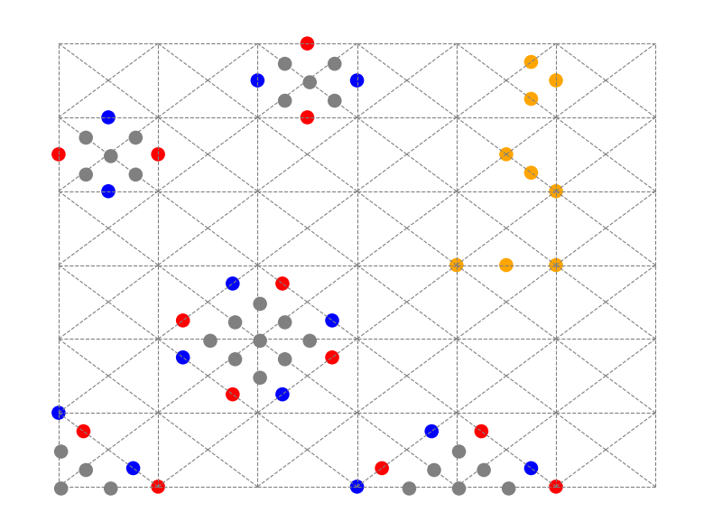
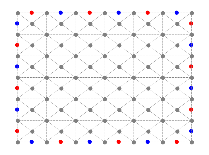
In the Pauli and qudit stabiliser formalisms, operators commute up to a phase. In the XP stabiliser formalism, operators commute up to a diagonal operator. This suggests that non-Abelian anyon models arise naturally in the XP formalism, and the existence of such codes in the XS stabiliser formalism had already been established in Ref. [18]. Such models may be useful in achieving fault-tolerant quantum computation [16] as well as understanding physical phenomena such as the fractional Quantum Hall Effect [24]. In Ref. [10], the authors showed that all twisted quantum doubles (TQDs) with Abelian anyons can be represented as qudit stabiliser codes. It would be interesting to see if there is a similar result for non-Abelian TQDs represented as XP codes. You can explore the logical operator structure of various topological codes, including Twisted Quantum Doubles, in the linked Jupyter notebook.
One of the most exciting implications of this work is that no-go theorems which apply to Pauli stabiliser codes and commuting stabiliser codes do not necessarily apply to XP codes. Such results exist, for instance, in the area of self-correcting quantum memories (Ref. [4] on page 23). Rather than rely on active error correction, a self-correcting quantum memory is a system where large scale errors would be suppressed by a macroscopic energy barrier. As XP codes involve stabilisers which are not Paulis and which may not commute, they are worth investigating for potential use as self-correcting memories.
Acknowledgements
This research was supported by the Australian Research Council via the Centre of Excellence in Engineered Quantum Systems (EQUS) project number CE170100009. BJB also received support from the European Union’s Horizon 2020 research and innovation programme under the Marie Skłodowska-Curie grant agreement No. 897158. Mark Webster was supported by the Sydney Quantum Academy, Sydney, NSW, Australia. We would also like to thank Paul Webster who reviewed early drafts of this paper and provided valuable feedback.
Appendix A Linear Algebra over Rings
Most readers will be familiar with linear algebra techniques for vector spaces over a field - for instance, solving linear equations or finding a basis of a subspace. In this paper, we work with vectors over , which is a ring in general rather than a field. Linear algebra over rings is not covered in standard linear algebra textbooks, so we give an introduction here (for more background, see Refs. [25] and [5]).
We start with basic concepts from ring theory in Section A.1. We then consider the row span of a matrix over a ring. For vector spaces, we can calculate the Reduced Row Echelon Form (RREF) of a matrix and this gives us a basis for the subspace spanned by the rows of the matrix. In Section A.2, we introduce the Howell matrix form which is a generalisation of the RREF for rings. Calculation of the Howell basis is central to many of the algorithms in this paper.
We show how to solve linear equations modulo in Section A.3 and how to find the intersection of spans in Section A.4. These techniques are used when calculating the logical operators of XP codes.
A.1 Ring Concepts
A ring is a set of elements with addition and multiplication binary operations. Elements of a ring are not guaranteed to have multiplicative inverses. Elements which do have inverses are called units. In contrast, a zero divisor is an element where for some .
We define an equivalence relation such that for some unit (or is an associate of ). For each element a of , we can calculate a minimal associate . We can show that .
Example A.1 (Ring Definitions for )
Using the ring as an example:
-
1.
The units are: .
-
2.
The zero divisors are:
-
3.
The minimal associates are:
| (193) |
Notice that if and only if is a unit.
A.2 Spans of Matrices and the Howell Matrix Form
We can define the span of a matrix with rows over a ring as:
| (194) |
Spans over rings can be considered subgroups of under component-wise addition over (i.e. ).
Where is a field (e.g. where is prime), the RREF gives us a basis of the span and two matrices have the same span if and only if they have the same RREF. The Howell form plays an analogous role for spans over rings.
The Howell matrix form or Howell basis of over a ring , denoted , is an matrix of form:
| (195) |
The entries of are subject to the following constraints:
-
•
Diagonal entries (marked above) are minimal associates in .
-
•
If the diagonal entry is zero, the whole row is zero
-
•
Entries below the diagonal entries are zero
-
•
Entries above the diagonal entries are strictly less than the diagonal entry (marked above), unless the diagonal entry is in which case they are unrestricted (marked above).
The Howell matrix is the unique matrix of the above form which has the Howell property. Let be the subset of where the first entries are zero. The matrix has the Howell property if is the span of the last rows of . Two matrices have the same span over if and only if they have the same Howell matrix. Methods of constructing the Howell matrix form of a given matrix are set out in Refs. [15], [25] and [5], and we use a simplified more intuitive algorithm in the XPF package. You can view examples of calculating the Howell matrix form in the linked Jupyter notebook.
Where is a field, . In the special case of binary matrices (i.e. where ), the RREF has a particular form. In particular, for any leading index the entries in column are strictly less than and hence are zero. This fact is useful when determining the special form of orbit representatives (see Section 4.3.2).
A.3 Solving Linear Equations over Rings
In this section, we show how to solve linear equations over rings using the Howell matrix form. Given the matrix and a constant vector , we wish to solve for the vector in the linear equation:
| (196) |
We calculate the Howell form of the transpose so that:
| (197) |
where and . As part of this calculation, we also obtain the Howell basis for such that . We can solve Eq. (196) if so that for some vector :
| (198) |
In this case, the solutions for are given by:
| (199) |
where ranges over all values of . That is a solution to Eq. (196) can easily be verified by substitution. We can also write the solution set as an affine span (see Eq. (200) below).
A.4 Intersections of Spans and Affine Spans
When calculating the codewords (Chapter 4) and logical operators (Chapter 6) of an XP code, we work with affine spans which can be identified with cosets of row spans. To find the logical X operators, we need to determine the intersection of affine spans (see Section E.2.3). In this section, we explain how to compute the intersection of two affine spans and introduce the residue function which identifies which coset a vector belongs to.
A.4.1 Affine Span Definition
Given an offset and a matrix , the affine span is defined as:
| (200) |
Because is a subgroup of , we can also consider affine spans to be cosets (i.e. ). The residue function identifies the coset of a vector and can be used to determine if two vectors are in the same affine span. The residue function is defined as:
| (201) |
A vector is in a span if and only if its residue is zero - i.e. . Vectors are in the same coset if and only their residues are the same - i.e. .
A.4.2 Algorithm for Intersection of Spans
Given two matrices and , we can find the intersection of the respective spans () as follows:
-
1.
Form the matrix
-
2.
Calculate the Howell basis of where is and is so that .
-
3.
Let .
-
4.
The intersection is
A.4.3 Algorithm for Intersection of Affine Spans
The intersection of two affine spans is either empty or an affine span. Assume we are given two affine spans and . There exists a vector in the intersection if and only if we can find vectors and such that:
| (202) |
This is possible only when which is true if and only if:
| (203) |
In this case, we set and the intersection is given by:
| (204) |
Appendix B Canonical Generator Algorithm - Proof of Result
In this appendix, we provide a proof of Proposition 4.1. This is an important result which states that we can calculate a set of canonical generators of unique form for any XP group. This allows us to determine whether two sets of XP operators generate the same group and also identify a set of generators for the diagonal subgroup. The proof of the proposition is constructive and relies on the following algorithm:
Canonical Generator Algorithm
The algorithm for producing the canonical generators from an arbitrary set of XP operators is:
-
1.
Simplify X Components: let be the binary matrix whose rows are the X components of the operators in . We can put into RREF by using row operations over . These row operations correspond to group operations between elements of and we update accordingly.
-
2.
Split into diagonal and non-diagonal operators: let be the non-diagonal operators and be the diagonal operators.
-
3.
Add squares and commutators of : squares and commutators of operators in are diagonal - add these to .
-
4.
Add commutators between and : add to all possible commutators between elements of and elements of . Where is a power of , we do this step times.
-
5.
Simplify : Let be matrix whose rows are the image of under the Zp map of Section 3.4 - i.e. . The final set of diagonal generators are the XP operators corresponding to the rows of i.e. .
-
6.
Simplify Z Components of : Let and let (see Eq. (201)). Replace with .
We restate Proposition 4.1 here for clarity:
Proposition 4.1 (Canonical Generators of an XP Group)
For any set of XP Operators , there exists a unique set of diagonal operators and non-diagonal operators with the following form:
-
1.
Let be the binary matrix formed from the X-components of the . is in Reduced Row Echelon Form (RREF).
- 2.
-
3.
For , is in Howell Matrix Form.
The following properties hold for the canonical generators:
Property 1:
All group elements can be expressed in the generator product form of Eq. (25) where , , and
Property 2:
Two sets of XP operators of precision generate the same group if and only if they have the same canonical generators.
Proof.
Steps 1-2 of the algorithm create a list of non-diagonal operators whose X-components are in RREF, plus diagonal operators . We claim that after these operations, . Over , the row operations to convert the matrix into RREF involve either:
-
1.
Swapping the order of rows; or
-
2.
Adding rows i.e.
The row operations can be translated into group operations on as follows:
-
1.
Swapping the order of generators; or
-
2.
Replacing a generator by a product of generators i.e. .
For case 2, we need to check if is still in the group after the row operations. Because is unchanged, remains in the group so we have .
Steps 3-4 of the algorithm ensure that all possible squares and commutators of the generators are added to the list of diagonal operators . Now we show that where , that rounds of adding commutators is sufficient. When we calculate the commutator of operators , the resulting degree (see Section 3.5) is at most half the degrees of : recall the COMM rule of Section 3.3:
| (205) |
As , the maximum degree of a precision operator is . Hence, after rounds of taking commutators, a further round of commutators yields operators of degree 1 (i.e. phase multiples of ). Note that all of the operators added to are in so there is no change to in this step.
Step 5 ensures that , the matrix formed from the phase and Z-components of under the Zp map is in Howell matrix form. In Section 3.4, we showed that the Zp map is a group homomorphism so group generators in , i.e. the rows of the Howell matrix, correspond to diagonal group generators in , i.e. so there is no change to the group generated by in this step.
In Step 6, the residue function of Eq. (201) ensures that the Z-components of the non-diagonal canonical generators are of the correct form. The adjustment corresponds to multiplication of elements in so we are assured that the final set of generators meets the invariant .
To prove Property 1, we need to show that any element can be expressed n the generator product form of Eq. (25) . We have already shown that . Hence, we can write as a string of operators from . Now assume we have a diagonal operator which occurs immediately before a non-diagonal operator . We can write:
| (206) |
The commutator , so we can always move diagonal operators to the right of non-diagonal operators.
Now assume we have two non-diagonal operators which occur immediately next to each other in the string, but out of order (i.e. ). We can move to the right of by using commutators as follows:
| (207) |
The commutator , so we can ensure occur in the correct order with a diagonal operator to the right.
Reordering the non-diagonal operators may result in squares or higher powers of non-diagonal operators arising in the string. As for any , any power of can be written as for odd or for some . Hence, can be written with powers of in . Accordingly, any can be written as a string of the form in Property 1.
To establish Property 2, note that the Howell matrix form and RREF are unique. Thus, for any operators which generate the same group, the canonical form will be the same. ∎
Appendix C Coset and Orbit Structure of Codewords
In Chapter 4, we gave an algorithm for generating the codewords by applying the orbit operator to the orbit representatives. In this appendix, we provide proofs underlying the algorithm. The results in this appendix assume we have the canonical generators and (see Section 4.1) and the set of binary vectors , which is the Z-support of the simultaneous eigenspace of (see Section 4.2.2). Our aim is to calculate a basis of the codespace stabilised by .
In Proposition C.1, we show that the image under the orbit operator of any where is stabilised by . Let be the binary matrix formed from the X-components of the and be the orbit representatives. In Proposition C.2, we show that is closed under addition by elements of the span . In Proposition C.3, we show that the cosets partition . In Proposition C.4, we show that the image of under the orbit operator forms a basis of the codespace. Finally, we show that the orbit representatives have a unique form, which is used in the graph search algorithm of Section 4.3.2.
Proposition C.1 (Codewords as Orbits)
Given canonical generators for a code and , let be the Z-support of the simultaneous eigenspace of .
Then is stabilised by all elements of , for any .
Proof.
It is sufficient to prove this for the generators and . Let be a diagonal generator. Then we have:
| (208) | ||||
| (209) | ||||
| (210) | ||||
| (211) |
Let be a non-diagonal operator.
| (212) |
We can move to the right by applying commutators. We can then move the commutators to the right. Let be the length binary vector which is all zero, apart from component which is 1 and let . As all commutators are diagonal and so are in , we can write:
| (213) | ||||
| (214) | ||||
| (215) |
∎
Proposition C.2 ( closed under addition by )
If , then for all .
Proof.
Let and . Then for some . Let and . Then because , and so:
| (216) |
Hence, is in the simultaneous eigenspace of the and so . ∎
Proposition C.3 (Cosets of partition )
The cosets partition i.e.:
| (217) | |||
| (218) |
Proof.
By Proposition C.2, for all hence . But by the definition of orbit representatives for any we can calculate hence for some .
The fact that cosets of a subgroup partition the group is a well-known result from group theory. Hence if then . But then because the RREF is unique so . ∎
Proposition C.4 (The are a basis of )
Let . The are a basis of the codespace stabilised by the canonical generators .
Proof.
First, we show that the are independent. The Z-support of the codeword is the coset and so by Proposition C.3 the Z-support of the codewords partition . Hence are independent.
Next, we show that the span the codespace . Let . Then is stabilised by all elements . Let then because is diagonal, and this implies . Hence .
Now let be the coefficients of in so that:
| (219) |
For , we now show that the coefficient is determined by the . Because , there exists unique such that The operator and so . The action of on is given by . Hence the coefficient of in is given by . Hence:
| (220) |
Hence any can be written as a linear combination of the and the result follows. ∎
The orbit representatives have a form which is unique for each coset, which proves useful in the graph search algorithm of Section 4.3.2.
Proposition C.5
Let be an binary matrix in RREF. Let be a binary vector of length and let . Then is the unique element of the coset for which for all leading indices of .
Proof.
We first show that for all leading indices of . By the definition in Eq. (201), the matrix is a binary matrix in Howell form. Hence, the entries above the leading indices are strictly less than and so are zero. Therefore for all leading indices .
Now we show the uniqueness of the property. Assume there exists some binary vector in the coset with for all leading indices . Then is a vector in such that for all leading indices of . The only member of with this property is hence . ∎
Appendix D Proof of Results: Classification of XP Stabiliser States
In this appendix, we provide detailed proofs of the results in Chapter 5. In Section D.1, we set out some basic results which are useful for working with integer and binary vectors. In Section D.2, we prove Proposition 5.1 regarding the form of the phase function of an XP stabiliser state. Finally in Section D.3, prove that the algorithm for representing weighted hypergraph states as XP stabiliser states gives the correct result.
D.1 Operations on Binary and Integer Vectors
The results in Chapter 5 involve operations on binary and integer vectors. This section sets out some basic results for these types of vectors. We use component wise addition and multiplication of vectors and a dot product of vectors over the integers. Given two vectors the dot product is defined as:
| (221) |
Hence, the dot product is the sum of the entries of the component wise product of two vectors. Accordingly, we can write the following rule for dot product over the component wise product:
| (222) |
We also have a distributive rule for dot product over component wise addition:
| (223) |
The usual rule for scalar products also applies - for :
| (224) |
The weight of a binary vector can also be thought of as a dot product. Let be the all 1 vector of length . Considering the binary vector a vector of zeros and ones in :
| (225) |
We can look at component wise multiplication and addition modulo 2 of binary vectors in terms of the effect on the support of the vectors. The support of the component wise product of binary vectors is the intersection of the supports:
| (226) |
The support of the addition of binary vectors modulo 2 is the symmetric difference of the supports:
| (227) |
We often apply the following identity for binary vectors:
| (228) |
where operations on the RHS are over the integers. This generalises to the following identity for binary vectors of length :
| (229) |
D.2 Phase Functions of XP Stabiliser States
In this section, we prove Proposition 5.1 which classifies the form of the phase functions of XP stabiliser states.
Proposition 5.1
[Phase Functions of XP States] Let be an XP stabiliser state in the canonical form of Eq. (50) with . Let be binary variables such that . Then:
-
(a)
The phase function is of the following form for some vector indexed by the subsets of :
(230) -
(b)
For , the maximum degree of the phase function is .
Proof.
Let and let . Using Eq. (229) and the dot product results of Section D.1, the phase component of can be written as follows:
| (231) | ||||
| (232) | ||||
| (233) | ||||
| (234) | ||||
| (235) |
The first term in the above equation is linear in and setting , the second term is also of the required form so part (a) follows.
Now let be a power of such that . As , any terms in the phase function with degree or have coefficients which are multiples of and hence generate trivial phases. Hence, the maximum degree of the phase function is and part (b) follows. ∎
D.3 Representing Weighted Hypergraph States as XP Stabiliser States
In this section, we show that the algorithm of Section 5.4 for representing weighted hypergraph states as XP stabiliser states produces the required results. The embedding operator of Eq. (57) is defined in terms of , which is the binary matrix whose columns are the bit strings of length of weight between and inclusive. This construction is similar to that used in classical simplex codes and Reed-Muller codes [3].
In the following proposition, we break into blocks where the columns all have weight and calculate the weight of the product of rows of .
Proposition D.1 (Weight of Vector Products)
Let be a matrix whose columns are the bit strings of length with weight . Let be the product of the first rows of where . Then:
| (236) |
Proof.
We can think of as the number of columns of such that . If then for all columns because and the product includes at least one zero.
If then the first entries in must all be one, implying that the last entries of must include values of 1. There are ways of constructing bit strings of weight which have the first entries equal to 1. ∎
We now consider dot products with the alternating vector of Eq. (58) which is 1 when the weight of the corresponding column of is even and when the weight is odd. The vector will be used to construct the Z-component of the non-diagonal stabilisers of the XP code.
Proposition D.2 (Dot Product with Alternating Vector)
Let be the th row of and let for . Let be the vector such that where is the th column of . Then if and otherwise.
Proof.
We now show that the alternating vector allows us to construct an XP stabiliser state which has a phase function corresponding to a generalised controlled phase operator.
Proposition D.3 (Weighted Hypergraph States)
Let be the th row of and let for and and as defined in Eq. (58). Let be the variable representing the value of for the binary vector of length . Then:
-
(a)
The operators commute; and
-
(b)
The phase component of is .
Proof.
(a) Using the COMM rule of Table 4, the group commutator of and is:
| (239) | ||||
| (240) | ||||
| (241) | ||||
| (242) |
We now show how to optimise the embedding operator to reduce the number of qubits required to represent the action of generalised controlled phase operators where :
Proposition D.4 (Weighted Hypergraph States - Optimised Version)
Proof.
Calculating the group commutator between two of the elements of :
| (245) | ||||
| (246) | ||||
| (247) | ||||
| (248) |
We now show that fixes all elements of the Z-support of . Let . Then using the notation of Proposition 5.1 and Eq. (229), the phase applied by to can be written
| (249) | ||||
| (250) | ||||
| (251) |
By Proposition D.2, if then . Similarly, if then . If , then a factor of always occurs - hence the operator applies a trivial phase and part (a) follows.
Due to Proposition D.2, we can multiply the generators by powers of without changing the phase function of the state , so part (b) follows. ∎
We now show how to apply Proposition D.4 to reduce the number of qubits required to represent as an XP stabiliser state. We set and let be the th row of . We define the non-diagonal stabiliser generators where - these are the same operators as in Proposition D.4. The phase function of is . This imparts a phase of when . Define the as in Eq. (62). By part (a) of Proposition D.4, the elements of commute up to a diagonal operator which fixes elements of the Z-support of hence stabilises .
To extend this method to generalised controlled Z operators of form , we need to ensure that for any other operator involved in the weighted hypergraph state. Otherwise, we cannot guarantee that the commutators of the operators in act trivially on the Z-support of the embedded state.
Appendix E Logical Operators - Proof of Results
In this appendix, we provide proofs for the main results in Chapter 6. We first prove two results about the properties of logical XP operators. We next show that the algorithms of Sections 6.2 and 6.3 produce valid logical operators, and that they produce all possible operators of XP form. We then show how to find valid phase and Z components for logical X operators. We then prove the observations of Example 6.4 regarding Reed-Muller codes. Finally, we prove that the more efficient algorithms of Section 6.6 work correctly.
E.1 Properties of Logical XP Operators
In this section, we prove two results on the properties of logical XP operators. Given the codewords of Section 4.4, the first result states that an XP operator is a logical operator if and only if its action on the codewords can be described in terms of:
-
•
A permutation of the codewords; and
-
•
A phase applied to each codeword
This result is used to prove that the logical operator and logical identity algorithms work correctly.
The second result states that an XP operator is a logical operator if and only if its commutators with logical identities are logical identities. It is an efficient way in practice to verify if an XP operator is a logical operator on the codespace.
Proposition E.1 (Action of Logical Operators)
An XP operator is a logical operator if and only if its action can be described by a permutation of the codewords such that and a vector specifying the phase applied to each codeword.
Proof.
Let be an XP operator. Applying the rule in Eq. (20), acts on computational basis elements as follows:
| (252) |
Hence, the image of a computational basis element under an XP operator cannot be a superposition of computational basis elements.
Now consider how acts on the codewords of Section 4.4. Let be the Z-support of the codeword and let be the number of non-diagonal canonical generators (i.e. ). Then and for . Hence, the image of a codeword under an XP operator cannot be a superposition of codewords.
Now assume is a logical operator and so preserves the codespace . As for each codeword and cannot create superpositions of codewords, then for some codeword and . Because the image of the codewords under must span the codespace, must permute the codewords. The square of any XP operator is diagonal (see Section 3.3) so the square of the permutation must be and the action of is as claimed. ∎
In the PSF, any logical operator on the codespace must commute with the stabiliser generators. In the XPF, we instead work with the generators of the logical identity group. The group commutator of a logical operator with each element of must be in the diagonal subgroup . In practice, this gives an efficient test for determining if a given operator is a logical operator on the codespace.
Proposition E.2 (Commutators Logical Operators and Logical Identities)
Let be the logical identity generators as in Section 6.2. is a logical XP operator if and only if .
Proof.
Assume , is a logical XP operator and are the codewords of Section 4.4. By Proposition E.1, there exists a phase vector and a permutation such that for all :
Hence so . From Section 3.3, we know that group commutators are always diagonal operators, hence .
Conversely, assume that . This is also true for any . Then for each codeword :
| (253) | ||||
| (254) |
Hence is in the codespace for all . Because is an XP operator cannot be a superposition of codewords and so for some and . Because is diagonal the map squares to and hence is a permutation. Therefore we can describe the action of as and so is a logical XP operator by Proposition E.1. ∎
E.2 Logical Identity and Logical Operator Algorithms
In this section, we prove that the logical identity algorithm of Section 6.2 and the logical operator algorithm of Section 6.3 yield generating sets of operators. We first consider the algorithms for diagonal operators, then those for non-diagonal operators. We then show how to find logical X operators by using the intersection of affine spans algorithm of Section A.4.
E.2.1 Diagonal Operator Algorithms
In this section, we show that the algorithms of Sections 6.3.1 and 6.2.1 produce sets of diagonal logical generators and diagonal logical identity generators respectively.
Assume we have the codewords in the orbit form of Eq. (35) - i.e. . Let be the Z-support of the codewords (see Section 4.2.2). We first look at diagonal logical identity operators and prove the following proposition:
Proposition E.3 (Diagonal Logical Identity Group)
The algorithm in Section 6.2.1 produces a list of diagonal XP operators which generate the diagonal logical identity XP operators for the codespace.
Proof.
The binary matrix is the matrix formed by taking as rows, where . If is a row of the Howell basis of , then . Let then . Hence, applies a trivial phase on each element of and hence on each codeword. Because , the generate all diagonal logical identity operators and so . ∎
We next look at the diagonal logical operators and show the following:
Proposition E.4 (Diagonal Logical Operators)
The algorithm in Section 6.3.1 produces a list of diagonal XP operators which together with and generate the diagonal logical XP operators for the codespace.
Proof.
We define the binary matrix used in the logical operator algorithm as follows. For each in Eq. (35), let be a binary vector of length which is all zeros apart from the th component which is . The vector is a “codeword index” that tells us which codeword the row belongs to. Let be the matrix formed by taking as rows. Let be the Howell basis of and let be a row of . Then for all values of and , and so .
Now consider how the diagonal XP operator acts on the Z-support of the codewords:
| (255) |
In other words, the action of is constant on the Z-support of each codeword and so is a logical operator with phase vector . The , together with the operator , generate all possible diagonal logical operators because .
We now show how to find non-trivial diagonal operators which together with and generate the same group as the and , reflecting steps 4 and 5 of the algorithm in Section 6.3.1. Because we include as a generator, we can just consider the space spanned by the Z components of the operators over . Let and be the matrices whose rows are the Z-components of the and respectively. For each row of we let so that for some vector . Let be the Howell basis of the matrix with the as rows. Then clearly . Letting then we have that . ∎
E.2.2 Non-diagonal Operator Algorithms
In this section, we show that the algorithms for non-diagonal operators yield valid logical operators and logical identities respectively. We then show that the operators produced are generating sets for the respective groups. Assume we have the coset decomposition of the Z-support of the codewords as in Eq. (119) i.e. . Recall that the rows of are the X-components of the non-diagonal canonical generators and that the binary vector if and only if (see Section 6.3.2).
Proposition E.5 (Non-diagonal Logical Operators)
Given a binary vector , the algorithm in Section 6.3.2 yields a non-diagonal logical operator with X-component equal to or FALSE if no such operator exists.
Proof.
Given and applying Proposition E.1, we wish to find for which for some phase vector and some permutation .
Because , we know that for orbit representatives . Define if . Then is a map which squares to and so is a permutation.
Now assume we have the codewords in the orbit format of Eq. (35). Let and let be the phase of in the codewords. We require that . Calculating the action of on :
| (256) |
The phase of is when:
| (257) |
As the phase is fixed for each codeword , for there to be a valid solution to be either even or odd for all . Let and . Define the vector . Hence:
| (258) |
Letting be the vector corresponding to the , we can write this in matrix form:
| (259) |
Solutions to this equation are members of the affine span (see Eq. (200)):
| (260) |
where is the Howell basis of and is a constant. We can either find or show that no solution exists by using linear algebra modulo (see Section A.3). If no such solution exists, return FALSE. Otherwise, the operator is the required non-diagonal logical operator. ∎
The algorithm for non-diagonal logical identity operators can be considered a special case of the algorithm for non-diagonal logical operators, with the matrix substituted for and the proof is omitted.
Corollary E.6 (Non-diagonal Logical Identity Group)
Given codewords in orbit format and , the algorithm in Section 6.2.2 yields a non-diagonal operator with X-component such that , or returns FALSE if no such operator exists.
We next show that the operators produced by the algorithms give us a generating set. We first show that the logical identity group is generated by the operators yielded by the logical identity algorithm.
Proposition E.7 (Logical Identity Group is Generated by )
The logical identity group for an XP code is the group generated by as calculated in Section 6.2:
| (261) |
Proof.
If then for all codewords by construction so , and so .
We now prove the converse. In Proposition E.3, we showed that generates the diagonal subgroup of
Let be a non-diagonal operator in . Then as defined above. Hence, we can find a binary vector such that . Let . Then and have the same component so . Then is a diagonal logical identity operator because both and are logical identities. Hence . Therefore . ∎
Finally, we show that the logical operators with X-components in , along with the stabiliser generators and the diagonal logical operators generate the entire logical operator group.
Proposition E.8
Let be the Z-support of the codewords of an XP code and let be the coset decomposition of as in Eq. (119). Let be the logical identity group as in Section 6.2, let be the set of diagonal operators as in Section 6.3.1 and let be a set of logical operators with X-components drawn from the rows of . Then the logical operator group is given by:
| (262) |
Proof.
Say we have a logical operator with a non-trivial X-component of the form . The action of on for is . We have shown that the codespace is spanned by the which have Z-support exactly equal to . Because logical operators preserve the codespace, X-components of logical operators must satisfy the constraint:
| (263) |
All possible X-components for logical operators are given by . To see this, assume there exists some meets the constraint in Eq. (263). Then meets the constraint in Eq. (263), which is a contradiction.
Next, we show that any logical operator can be written as where has X-component in and . We know that so for some binary vectors . Let then is a logical operator with X component in .
Now assume that there are two different logical operators with X-component - say and . The product is a diagonal logical operator so is the same as up to a product of a diagonal logical operator. Applying Proposition E.4,
Accordingly, we can generate all possible logical operators by finding the non-diagonal logical operators with X-components in . Together with the logical identity generators , and , these generate the full set of logical operators. ∎
E.2.3 Diagonal Component of Logical X Operators
We have demonstrated how to find a non-diagonal logical operator with X-component in . This will not necessarily act as a logical X operator. In particular, a logical X should square to a logical identity and in this section, we show how to ensure that this is the case.
Assume we have used the algorithm in Section 6.3.2 to find a logical operator . Our aim is to calculate a logical X operator such that is a logical identity. As is diagonal, we require . Our strategy is to first find the Z component of , then adjust the phase component.
We first look at which Z components are possible for logical operators with the same X component as . We can multiply by any diagonal logical operator in and get a logical operator, and all possible Z components of such operators arise in this way. Let be the matrices formed from the Z components of respectively. Writing , the possible Z components are given by the affine span:
| (264) |
We next address the condition that the Z component of , which we denote here, has to be in . By applying the square rule of Section 3.3:
| (265) |
When . Hence, has to be an element of which is zero when . Because is the Z component of a square, we also know that it is a multiple of . Hence . All generators of are divisible by 2, so let be the span with generators from divided by . Any will have .
Where the precision is a multiple of 2 and , adding to does not change whether because . Hence, we can add any element of to .
We can add any element of to and still ensure because where , is guaranteed to be zero. Hence when defined as:
| (266) |
Hence, . If this span is not empty then we can find such that for some vector . Let be the phase components of and respectively. We set the phase component of to be .
E.3 Reed-Muller Codes
Reed-Muller codes are well-known Pauli Stabiliser codes. We can also look at them as XP codes and better understand their logical operator structure. In the Proposition below, we show that they are self-dual codes and have transversal logical operators at precision . To demonstrate the results, we apply the techniques of Appendix D.
Proposition E.9 (Reed-Muller XP Codes)
The Reed-Muller code on qubits can be written as the codespace of a precision code whose stabiliser generators are symmetric in X and P. The code has a transversal logical operator.
Proof.
Let and the number of qubits . Let and where is the th row of as in Section 5.4. Let and let where is the vector of length with all entries .
We claim that the codespace of is spanned by . For this, we need to show that the simultaneous +1 eigenspace of the is given by where . Let and let . Note that . Hence we need to show that .
Applying Proposition D.1 the weight of the product of distinct is because:
| (267) |
Now consider the dot product of with and apply Eq. (229):
| (268) |
By setting in Eq. (267) we see that . Hence:
| (269) |
Now rescale the code to precision consider the action of on and . We can write . Now . Calculating :
| (270) |
Hence, the phase applied by to each basis element making up is trivial and so .
The action of on is . The phase component of is . Hence and acts as a logical operator. ∎
E.4 Modified Algorithms for Logical Identity Group and Logical Operators
Our objective here is to show that where , we can calculate the logical identity group and logical operators without first calculating the codewords in full. Assume that the codewords in orbit form are as in Eq. (35) and let be the Z-support of the codewords.
-
•
To calculate the logical identity group generators, we just need to consider the elements of at most orbit distance from the core elements .
-
•
For the logical operators, we need to consider the elements of at most orbit distance from the orbit representatives .
We need a number of preliminary results to prove the main propositions. In these results, we work with a binary matrix in RREF. Let the rows of be the binary vectors . Sums and products of vectors are component wise in (i.e. ).
We first write an expression for the sum modulo 2 of a subset of the :
Lemma E.10
Let be a binary matrix in RREF, with non-zero rows and let . Define:
| (271) |
and for define :
| (272) |
then:
| (273) |
where we work in on the RHS.
Proof.
Induction on .
Base Step:
Induction Step:
Assume and the lemma is true for any sets . Let and . For binary vectors :
| (276) |
Hence, the LHS of Eq. (273) is:
| (277) |
Because , we can apply the induction hypothesis:
| (278) | ||||
| (279) | ||||
| (280) |
The induction step holds and the result follows. ∎
Next, we let and consider spans over of the binary vectors . We first show that certain products are in the span:
Lemma E.11 (Products of of Degree )
Let be a set of binary vectors with coset decomposition as in Eq. (119). Let the nonzero rows of be . Let where . Let be the elements of at most orbit distance from so that . Let and let . Then:
| (281) |
Proof.
Induction on .
Base Case:
let so that . Then:
| (282) |
As , and so is (as it is of orbit distance 0). Hence the linear combination is in and the base case holds.
Induction Step:
Assume and that the lemma is true for any sets . As , the binary vector . Expanding the expression for using Eq. (273):
| (283) | ||||
| (284) | ||||
| (285) |
By the induction hypothesis for any . As are also in the span, the induction step holds. ∎
We next show that the product of up to of the binary vectors is in :
Corollary E.12 (Products of of Degree )
Let and be defined as in Lemma E.11. Then:
| (286) |
Proof.
For , we have shown in Lemma E.11 that . Expanding the second we have:
| (287) |
As the span is over , any multiples of can be disregarded so . ∎
The results for the modified algorithms follow directly from the following proposition:
Proposition E.13
Let be as in Lemma E.11. Then:
| (288) |
Proof.
Let . Let . Using Eq. (273) we can write:
| (289) | ||||
| (290) | ||||
| (291) | ||||
| (292) |
We can disregard any multiples of so we can write:
| (293) |
By Lemma E.11 and Corollary E.12, we know that all elements on the RHS are in hence . Hence, all linear combinations of elements of are also in the span and the result follows. ∎
The main results of the section now follow by application of the previous proposition:
Proposition E.14 (Modified Logical Identity Algorithm)
Let be as defined in the algorithm of Section 6.2.1 i.e. the rows of are the binary vectors , plus a final column of all ’s. Let and be the elements of of orbit distance at most from the core . Let be the matrix formed from the rows of plus a row of ’s. Then:
| (294) |
Proof.
Let be the coset decomposition of . Let be the vectors in with an appended 1 (i.e. . Let and let be with an appended 0 so . Then . The result follows by applying Proposition E.13. ∎
Proposition E.15 (Modified Logical Operator Algorithm)
Let be as defined as in the algorithm of Section 6.3.1 i.e. the rows of are the binary vectors , plus a codeword index which identifies which codeword the row belongs to. Let and be the elements of of orbit distance at most from the orbit representatives . Let be the matrix formed from the rows of plus the codeword index. Then:
| (295) |
Appendix F Measurements in the XP Formalism - Proof of Results
In this appendix, we prove the results discussed in Chapter 7. We first prove the results for determining the outcome probabilities for measurement of XP operators. We then explain the stabiliser algorithm for measurement of diagonal Pauli operators of Section 7.3.2.
F.1 Measurement Outcome Probabilities - Proof of Results
In this section, we show how to determine the outcome probabilities for measurement of XP operators assuming we are given the codewords in the orbit form of Eq. (35). We first show how to determine probabilities for measurement of diagonal operators, then look at non-diagonal operators.
Proposition F.1 (Outcome Probabilities - Diagonal XP Operators)
Let be a diagonal XP operator which has as an eigenvalue. Let be the Z-support of the codewords . Let be the set of binary vectors . Let be an even superposition of the codewords as in Eq. (166) so that . The probability of obtaining outcome when measuring on is:
| (296) |
Proof.
Let the projector onto the eigenspace of be and let . The probability of obtaining outcome is .
Applying Eq. (22) with , the action of the projector on a computational basis vectors is given by:
| (297) |
Let . The action of on the codeword is:
| (298) | ||||
| (299) |
The result follows by noting that and . ∎
Proposition F.2 (Outcome Probabilities - Non-diagonal XP Operators)
Let be an even superposition of the codewords as in Eq. (166). Let be a non-diagonal XP operator with eigenvalue . Let be the Z-support of the codewords as calculated in Chapter 4 and let be the canonical non-diagonal generators as in Section 4.1. Let be the set of binary vectors .
If there exists with the same X-component as then let and let . The probability of obtaining outcome when measuring on is:
| (300) |
Proof.
Let be the operator we wish to measure, and assume we obtain outcome . Applying Eq. (23) with , the action of on a basis vector is:
| (301) |
Any elements where will be eliminated, so let:
| (302) |
By calculating , we can determine if there exists some with the same X-component as . There are two possible cases:
Case 1: does not exist:
Case 2: exists:
Let be the element of with the same X-component as and let so that . Let and for some phases . Then with relative phase . Consider the effect of the projector on :
| (305) | ||||
| (306) | ||||
| (307) | ||||
| (308) |
Now we determine :
| (309) | ||||
| (310) | ||||
| (311) |
Let , let and let . Then . Hence:
| (312) |
The result follows by noting that and . ∎
F.2 Analysis of Algorithm for Measuring Diagonal Paulis
In this section, we explain why the algorithm of Section 7.3.2 for measurement of diagonal Pauli operators works. We also consider implications for the complexity of measuring higher precision diagonal operators.
Firstly, we show that simulating the measurement of a diagonal Pauli operator reduces to determining the change in the Z-support of the codewords . Let and let be the codewords of the code in orbit format of Eq. (35) with Z-support . Let be the projector onto the eigenspace of . The action of on is given by Eq. (22):
| (313) |
Hence, the Z-support of the codewords after measurement outcome is . As is of precision 2, the action of on is . Hence . From Proposition F.1, the probability of obtaining outcome is and the phase of any remaining in the codewords is unchanged. Similarly, the Z-support of the codewords after obtaining outcome is with probability . Therefore, we can simulate measurement by determining and which in turn requires us to determine for all .
Next, we show how the algorithm in Section 7.3.2 correctly determines . To calculate , we need to determine for all . For any binary vectors , taking parity with respect to commutes with taking the sum modulo 2. That is:
| (314) |
Looking at Step 1 of the algorithm, assume there exists operators with X-components such that . Then the X-component of is and from Eq. (314), we know that . Hence, updating in Step 1 ensures that , for all X-components of the updated set . We remove from so updating by adding vectors of form to ensures that is unchanged ( are the matrices formed from the X-components of respectively).
Now looking at Step 2 of the algorithm, we can express the binary vectors as linear combinations modulo i.e. (see Section 6.4). After Step 1, we have ensured that , for all . Linear combinations of the also have parity and so the parity of is the same as the parity of because:
| (315) |
So is in if only if which is equivalent to . Let then . Hence, the probability of obtaining outcome is . By a similar argument, the result for the outcome is also correct.
The underlying reason the algorithm works is that the parity function of Eq. (167) commutes with addition of vectors modulo . Hence, the parity of the binary vector labelled in accordance with the quantum numbers of 6.4 is the same as the parity of (see Eq. (315)). This relationship breaks down for higher precision XP operators (e.g. ).
References
- Aaronson and Gottesman [2004] Scott Aaronson and Daniel Gottesman. Improved simulation of stabilizer circuits. Phys. Rev. A, 70:052328, Nov 2004. doi: 10.1103/PhysRevA.70.052328.
- Bermejo-Vega and Van Den Nest [2014] Juan Bermejo-Vega and Maarten Van Den Nest. Classical simulations of abelian-group normalizer circuits with intermediate measurements. Quantum Info. Comput., 14(3–4):181–216, Mar 2014. ISSN 1533-7146. doi: 10.26421/QIC14.3-4-1.
- Bierbrauer [2016] Juergen Bierbrauer. Introduction to coding theory. Discrete mathematics and its applications. Taylor and Francis, Boca Raton, second edition, Sep 2016. ISBN 9781315371993. doi: 10.1201/9781315371993.
- Brown et al. [2016] Benjamin J. Brown, Daniel Loss, Jiannis K. Pachos, Chris N. Self, and James R. Wootton. Quantum memories at finite temperature. Rev. Mod. Phys., 88:045005, Nov 2016. doi: 10.1103/RevModPhys.88.045005.
- Buchmann and Neis [1996] Johannes Buchmann and Stefan Neis. Algorithms for linear algebra problems over principal ideal rings. Technical Report TI-7/96, TU Darmstadt, Jan 1996. URL http://tubiblio.ulb.tu-darmstadt.de/101111/.
- Campbell [2016] Earl T. Campbell. The smallest interesting colour code. Blog Post, Sep 2016. URL https://earltcampbell.com/2016/09/26/the-smallest-interesting-colour-code/.
- Cross et al. [2009] Andrew Cross, Graeme Smith, John A. Smolin, and Bei Zeng. Codeword stabilized quantum codes. IEEE Transactions on Information Theory, 55(1):433–438, Aug 2009. doi: 10.1109/TIT.2008.2008136.
- de la Fuente et al. [2021] Julio Carlos Magdalena de la Fuente, Nicolas Tarantino, and Jens Eisert. Non-Pauli topological stabilizer codes from twisted quantum doubles. Quantum, 5:398, Feb 2021. doi: 10.22331/q-2021-02-17-398.
- Deutsch [1989] David Elieser Deutsch. Quantum computational networks. Proceedings of the Royal Society of London. Series A, Mathematical and physical sciences, 425(1868):73–90, Sep 1989. ISSN 1364-5021. doi: 10.1098/rspa.1989.0099.
- Ellison et al. [2021] Tyler D. Ellison, Yu-An Chen, Arpit Dua, Wilbur E. Shirley, Nathanan Tantivasadakarn, and Dominic J. Williamson. Pauli stabilizer models of twisted quantum doubles. arXiv:2112.11394 [quant-ph], Dec 2021. doi: 10.48550/arXiv.2112.11394.
- Gheorghiu [2014] Vlad Gheorghiu. Standard form of qudit stabilizer groups. Physics Letters A, 378(5):505–509, Jan 2014. ISSN 0375-9601. doi: 10.1016/j.physleta.2013.12.009.
- Gottesman [1998] D Gottesman. The Heisenberg representation of quantum computers. arXiv:quant-ph/9807006, Jun 1998.
- Gross et al. [2007] D. Gross, J. Eisert, N. Schuch, and D. Perez-Garcia. Measurement-based quantum computation beyond the one-way model. Phys. Rev. A, 76:052315, Nov 2007. doi: 10.1103/PhysRevA.76.052315.
- Hartmann et al. [2007] L Hartmann, J Calsamiglia, W Dür, and H J Briegel. Weighted graph states and applications to spin chains, lattices and gases. Journal of Physics B: Atomic, Molecular and Optical Physics, 40(9):S1–S44, Apr 2007. doi: 10.1088/0953-4075/40/9/s01.
- Howell [1986] John A. Howell. Spans in the module . Linear and Multilinear Algebra, 19(1):67–77, Jan 1986. doi: 10.1080/03081088608817705.
- Kitaev [2003] A.Yu Kitaev. Fault-tolerant quantum computation by anyons. Annals of physics, 303(1):2–30, Jan 2003. ISSN 0003-4916. doi: 10.1016/S0003-4916(02)00018-0.
- Miller and Miyake [2016] Jacob Miller and Akimasa Miyake. Hierarchy of universal entanglement in 2D measurement-based quantum computation. npj Quantum Information, 2:16036, Nov 2016. doi: 10.1038/npjqi.2016.36.
- Ni et al. [2015] Xiaotong Ni, Oliver Buerschaper, and Maarten Van den Nest. A non-commuting stabilizer formalism. Journal of Mathematical Physics, 56(5):052201, May 2015. doi: 10.1063/1.4920923.
- Nielsen and Chuang [2010] Michael A. Nielsen and Isaac L. Chuang. Quantum Computation and Quantum Information: 10th Anniversary Edition. Cambridge University Press, Dec 2010. doi: 10.1017/CBO9780511976667.
- Orús [2014] Román Orús. A practical introduction to tensor networks: Matrix product states and projected entangled pair states. Annals of Physics, 349:117–158, Oct 2014. ISSN 0003-4916. doi: 10.1016/j.aop.2014.06.013.
- Rains et al. [1997] Eric M. Rains, R. H. Hardin, Peter W. Shor, and N. J. A. Sloane. A nonadditive quantum code. Phys. Rev. Lett., 79:953–954, Aug 1997. doi: 10.1103/PhysRevLett.79.953.
- Rengaswamy et al. [2020] Narayanan Rengaswamy, Robert Calderbank, Michael Newman, and Henry D. Pfister. On optimality of CSS codes for transversal T. IEEE Journal on Selected Areas in Information Theory, 1(2):499–514, Aug 2020. doi: 10.1109/JSAIT.2020.3012914.
- Rossi et al. [2013] M Rossi, M Huber, D Bruß, and C Macchiavello. Quantum hypergraph states. New Journal of Physics, 15(11):113022, Nov 2013. doi: 10.1088/1367-2630/15/11/113022.
- Stern [2008] Ady Stern. Anyons and the quantum Hall effect—a pedagogical review. Annals of Physics, 323(1):204–249, Jan 2008. ISSN 0003-4916. doi: 10.1016/j.aop.2007.10.008.
- Storjohann [2000] Arne Storjohann. Algorithms for Matrix Canonical Forms. PhD thesis, Department of Computer Science, Swiss Federal Institute of Technology – ETH, 2000. URL https://cs.uwaterloo.ca/~astorjoh/diss2up.pdf.
- Van den Nest et al. [2004] Maarten Van den Nest, Jeroen Dehaene, and Bart De Moor. Graphical description of the action of local Clifford transformations on graph states. Phys. Rev. A, 69:022316, Feb 2004. doi: 10.1103/PhysRevA.69.022316.
