Distributed Randomized Kaczmarz for the adversarial workers

Abstract

Developing large-scale distributed methods that are robust to the presence of adversarial or corrupted workers is an important part of making such methods practical for real-world problems. Here, we propose an iterative approach that is adversary-tolerant for least-squares problems. The algorithm utilizes simple statistics to guarantee convergence and is capable of learning the adversarial distributions. Additionally, the efficiency of the proposed method is shown in simulations in the presence of adversaries. The results demonstrate the great capability of such methods to tolerate different levels of adversary rates and to identify the erroneous workers with high accuracy.

1 Introduction

It is critical for machine learning algorithms and their optimization subroutines to be robust and adversary-tolerant. A common approach is to utilize redundancy; that is, to request the same computation from multiple workers. The main challenge with such an approach is to leverage the outputs from these workers efficiently, and in such a way that even seemingly catastrophic adversarial outputs can be identified and tolerated.

In this work, our goal is to develop a variation of the randomized Kaczmarz (RK) method (Strohmer and Vershynin, 2009) (see Algorithm 1) for adversarial workers to solve the linear system $Ax=b$, where $A\in\mathbb{R}^{m\times n}$, $x\in\mathbb{R}^{n}$ and $b\in\mathbb{R}^{m}$. We assume that there is one central server $w_{c}$ and $N$ workers in total, among which $p$ fraction of the workers are adversarial (and unknown).

Algorithm 1 Randomized Kaczmarz Algorithm

  Select a row index $i_{j}\in[m]$ with probability $p_{i_{j}}=\frac{\|A_{i_{j}}\|_{2}^{2}}{\|A\|_{F}^{2}}$

  Update $x_{j+1}=\arg\min_{x\in\mathbb{R}^{n}}\|x-x_{j}\|$

  s.t. $A_{i_{j}}x_{j+1}=b_{i_{j}}$

  Repeat until convergence

Our approach utilizes simple statistics to identify and ignore adversarial “errors”, and thus the setting in which the adversaries communicate and select among $k$ types of errors to output is the most challenging for our approach. To implement our RK Algorithm, the central server randomly chooses a row index $i$ and broadcasts the data $A_{i}$ ($i$th row of $A$), $b[i]$ ($i$th entry of $b$) and $x_{j}$ (current estimate) to $n$ randomly chosen workers at each step. The workers that belong to the $\ell$-th category $C_{\ell}$ take up $p_{\ell}$ fraction of all workers, and $\sum_{\ell=1}^{k}p_{\ell}=p$. An adversarial worker $s$ in category $C_{\ell}$ returns $r_{s}=b[i]+e_{\ell}-\langle x_{j},A_{i}\rangle$ and a reliable worker returns $r_{s}=b[i]-\langle x_{j},A_{i}\rangle$.

1.1 Contribution

Our main contributions are threefold: (i) develop several efficient algorithms to guarantee accurate estimates for the true solution when adversaries are present, (ii) learn the adversary rate and find the adversarial workers efficiently, (iii) provide theoretical convergence analysis with adversarial workers.

1.2 Related work

Kaczmarz method.  The Kaczmarz method is an iterative method for solving linear systems that was first proposed by Kaczmarz (1937) which is also known under the name Algeberaic Reconstruction Technique (ART) in computer tomography (Gordon et al., 1975; Herman and Meyer, 1993; Natterer, 2001) and has found various applications ranging from computer tomography to digital signal processing. Later Strohmer and Vershynin (2009) propose a randomized version of Kaczmarz, where the the probability of each row being selected is set to be proportional to the Euclidean norm of the row and prove the exponential bound on the expected rate of convergence. In Needell (2009), the author proves that RK converges for inconsistent linear systems to a horizon that depends upon the size of the largest entry of the noise.

Distributed computing.  In the distributed computation, potential threats are the non-responsive workers (also known as stragglers) and adversarial workers. To mitigate the issues with straggling workers (Gordon et al., 1970; Karakus et al., 2017) introduce several encoding schemes that embed the redundancy directly in the data itself. Later, Bitar et al. (2020) propose an approximate gradient coding scheme for straggler mitigation when the stragglers are random. To deal with adversarial workers, Yang and Bajwa (2019) propose a variant of the gradient descent method based on the geometric median in the setting where the workers split all the data. Alistarh et al. (2018) discuss the problem of stochastic optimization in an adversarial setting where the workers sample data from a distribution and an $\alpha$ fraction of them may adversarially return any vector. These methods either have fundamental statistical barriers to the error any algorithm can achieve or works only when the adversary rate $\alpha$ is less than $\frac{1}{2}$, whereas our algorithm is able to converge to the exact solution even with an adversary rate higher than $\frac{1}{2}$ by utilizing redundancy.

2 Algorithm

2.1 Algorithms

In this section, we introduce a simple but efficient mode-based algorithm to effectively solve linear systems in the presence of the adversarial workers and identify the potential adversarial workers (which are put in a block-list). The method detects the mode category based on the returned category size. More specifically, the central worker groups the same results and update the guess with the results from the group with the largest size (i.e., mode). Given $n$ workers, the expected number of workers from $C_{\ell}$ is ${np_{\ell}}$ and number of non-adversarial workers is $n(1-p)$. In practice, we randomly choose a group with the maximum group size, its results will be used to update the guess as long as the group size is greater than $n(1-p)$ (see Alg. 2 Line 7). Meanwhile, the block-list is updated through a frequency-based approach throughout the iterations: a counter records if a worker’s result fails to be the mode during each iteration and after certain number of iterations, a threshold is applied to the counter to identify the potential adversarial workers (see Alg. 2 Line 9 - 11) Once a worker is in the block-list, it will not be visited again. We present the full details in Alg. 2. In the sequel, the theoretical results are based on Alg. 2.

Algorithm 2 Distributed Randomized Kaczmarz with block list

1:  Input: Initialize block-list $B$, good worker set $D=[N]$, a counter vector $E=0\in\mathbb{R}^{n}$, MaxIter, Tol, $c_{s}=2~{}\text{Tol}$, checking period $T$.

2:  while $j<\text{MaxIter}$ and $|c_{s}|>\text{Tol}$,  do

3:     The central worker $w_{c}$ selects a row index $i_{j}\in[m]$ with probability $p_{i_{j}}=\frac{\|A_{i_{j}}\|_{2}^{2}}{\|A\|_{F}^{2}}$

4:     Sample $w_{1},\cdots,w_{n}$ uniformly from $D$

5:     Broadcast $A_{i_{j}}$ to $w_{1},\cdots,w_{n}$

6:     $w_{s}$ returns $c_{s}=\frac{\langle A_{i_{j}},x_{i}\rangle-b_{i_{j}}}{\|A_{i_{j}}\|^{2}}+e_{l}$, if $w_{s}\in C_{l}$

7:     $w_{c}$ splits $\{c_{s}\}_{s=1}^{n}$ into groups $G_{1},\cdots,G_{k}$ and randomly choose from groups $G_{s}$ that satisfy $|G_{s}|\geq n(1-p)$

8:     Update $x^{j+1}=x^{j}+c_{s_{0}}A_{i_{j}}^{\top}$

9:     Update $E(s)=E(s)+1,$ if $c_{s}\notin G_{s_{0}}$

10:     if mod$(j,T)=0$ then

11:        Update $B$ by checking the value of entries in $E$

12:        $D=D\setminus B$

13:     end if

14:     Update $j=j+1$

15:  end while

16:  Output: $x^{j}$ and $B$

3 Theoretical Results

In this section, we study the mode distributions and convergence of Algorithm 2 from a theoretical perspective. For the reader’s convenience, we first summarize some important notation in Table 1.

$N$	Number of workers in total
$n$	Number of workers used in each iteration
$C_{\ell}$	$\ell$-th error category
$p$	Error ratio
$p_{\ell}$	Error ratio in category $C_{\ell}$
$q$	Probability that there is a mode among the outputs of $n$ chosen workers
$q_{\ell}$	probability that there is a mode among the outputs of $n$ chosen workers and the mode is in the category $\ell$
$k$	Number of adversarial categories

Table 1: Notation

3.1 Adversary Rate Learning

Alg. 2 utilizes the mode to identify adversaries and achieve convergence. In this section, we will compute the probability that category $\ell$ is the mode during each iteration. For simplicity, let $C_{0}$ denote the category which consists of the “good” workers and its fraction is denoted by $p_{0}=1-p$. We set $i_{0}=\max(\lceil\frac{n}{k+1}\rceil,\lceil n(1-p)\rceil)$. First, we denote $a_{i,\ell}$ as the coefficients of the term $x^{n-i}$ in the polynomials $\prod\limits_{r=0,r\neq\ell}^{k}q_{i}^{r}(x)$ for $\ell=0,\cdots,k$, where

$$q_{i}^{\ell}(x) = \sum_{j=0}^{i-1}\binom{Np_{\ell}}{j}x^{j}.$$

Let $N$ be the number of total workers, $p_{\ell}$ be the fraction of the category $\ell$, $k$ be the number of error types. Then the mode distributions can be summarized as follows.

Theorem 3.1.

If we choose $n$ workers from $N$ workers uniformly , then the probability that the mode is in the category $\ell$ is:

$$\hat{q}_{mode}^{\ell}=\sum_{i=i_{0}}^{n}\frac{\binom{Np_{\ell}}{i}a_{i,\ell}}{\binom{N}{n}}.$$

Thus the probability that there is a mode is:

$$q= \sum_{\ell=0}^{k}\hat{q}_{mode}^{\ell}=\sum_{i=i_{0}}^{n}\sum_{l=0}^{k}\frac{\binom{Np_{\ell}}{i}a_{i,\ell}}{\binom{N}{n}},$$

where $\binom{n}{i}=0$ when $n<i$.

Next, let’s consider the probability that a specific worker in category $\ell$ is chosen as a mode worker.

Theorem 3.2.

If we randomly choose $n$ workers from $N$ workers uniformly, then the probability that the worker $w$ in category $\ell$ is not mode for $s$ times over $S$ iterations is

$$\binom{S}{s}\left(1-P(w,q_{mode}^{\ell})\right)^{s}(1-\frac{1}{N}+P(w,q_{mode}^{\ell}))^{(S-s)}$$

where $P(w,q_{mode}^{\ell})=P(w)P(w\text{ is mode}|w)$ with

$$P(w\text{ is mode}|w)=\sum_{i=i_{0}-1}^{n-1}\frac{\binom{Np_{\ell}-1}{i}a_{i,\ell}}{\binom{N-1}{n-1}},P(w)=\frac{\binom{N-1}{n-1}}{\binom{N}{n}}.$$

3.2 Convergence Guarantee

Theorem 3.3.

Let $A\in\mathbb{R}^{d_{1}\times d_{2}}$ with $d_{1}\geq d_{2}$ and $b,e_{1},\cdots,e_{k}\in\mathbb{R}^{d_{1}}$. Assume that we solve $Ax^{*}=b$ via Algorithm 2, then

$$\mathbb{E}\|x_{i+1}-x^{*}\|_{2}^{2}\leq \alpha^{i+1}\|x_{0}-x^{*}\|_{2}^{2}$$ (1)

$$+\frac{1-\alpha^{i+1}}{1-\alpha}\frac{1}{\|A\|_{F}^{2}}\sum_{\ell=1}^{k}q_{\ell}\|e_{\ell}\|^{2},$$

where $\sigma_{\min}^{2}(A)$ is the smallest singular value of $A$, $\alpha=1-\frac{\sigma_{\min}^{2}(A)}{\|A\|_{F}^{2}}$ and $q_{\ell}=\frac{\hat{q}^{l}_{mode}}{q}$.
Additionally, if $\|e_{\ell}\|\leq C$, we thus have

$$\mathbb{E}\|x_{i+1}-x^{*}\|_{2}^{2}$$ (2)

$$\leq \alpha^{i+1}\|x_{0}-x^{*}\|_{2}^{2}+\frac{1-\alpha^{i+1}}{1-\alpha}\frac{Cq_{0}}{\|A\|_{F}^{2}}.$$

In the second half of this theorem, we use the fact that $\sum_{\ell=0}^{k}q_{\ell}=1$. Furthermore, we could assume that $\mathbb{E}\|e_{\ell}\|^{2}=d\sigma_{\ell}^{2}$ at each iteration.

To provide a quantitative understanding of Theorem 3.3, we present several examples in Tables 2 and 3 and for simplicity, assume that each error category has the same fraction $p_{\ell}=p/k$. Thus, all $\hat{q}_{mode}^{\ell}$ are equal. Here $q_{0}$ is the probability that the algorithm chooses the right mode and $q$ is the probability that there is a mode. Table 2 shows the probability $q$ and $q_{\ell}$. In these two tables, we present the values for $\hat{q}_{mode}^{\ell},\hat{q}_{mode}^{0},q$ and $q_{0}$ by varying the number of error types $k$, the number of chosen workers $n$ and the adversarial rate $p$. These two tables are generated by solving a linear system with a row-normalized matrix $A\in\mathbb{R}^{1000\times 100}$. As $k$ increases, $q_{\ell}$ decreases and $q_{0}$ increases. Therefore, the error bound in equation (2) decreases with respect to $k$ and thus reaches better convergence results. When $k$ is large enough, $q_{\ell}\approx 0$. Therefore, when the noise is random error and there is a mode for the step-size, the mode will be the correct mode. As $n$ increases, there is a similar decrease effect and therefore a better convergence.

$p$	$k$	$\hat{q}_{mode}^{\ell}$	$\hat{q}_{mode}^{0}$	$q$	$q_{0}$
$0.8$	$5$	$0.1$	$0.16$	$0.67$	$0.15$
	$10$	$0.04$	$0.21$	$0.57$	$0.36$
	$15$	$0.02$	$0.23$	$0.48$	$0.46$
$0.2$	$3$	$0.002$	$0.63$	$0.64$	$0.98$
	$5$	$8\times 10^{-4}$	$0.65$	$0.65$	$0.99$
	$10$	$2\times 10^{-4}$	$0.66$	$0.67$	$0.99$
	$15$	$2\times 10^{-4}$	$0.685$	$0.689$	$0.99$

Table 2: Total number of workers $N=100$, number of chosen workers $n=5$.

$p$	$n$	$\hat{q}_{mode}^{\ell}$	$\hat{q}_{mode}^{0}$	$q$	$q_{0}$
$0.8$	10	0.099	0.18	0.67	0.26
	15	0.099	0.2	0.7	0.29
	20	0.097	0.23	0.71	0.31
$0.2$	10	$7\times 10^{-6}$	0.904	0.90	$1-5\times 10^{-6}$
	15	$5\times 10^{-7}$	0.97	0.97	$1-3\times 10^{-6}$
	20	$1\times 10^{-7}$	0.99	0.99	$1-6\times 10^{-7}$

Table 3: Total number of workers $N=100$, number of error categories $k=5$.

4 Simulation

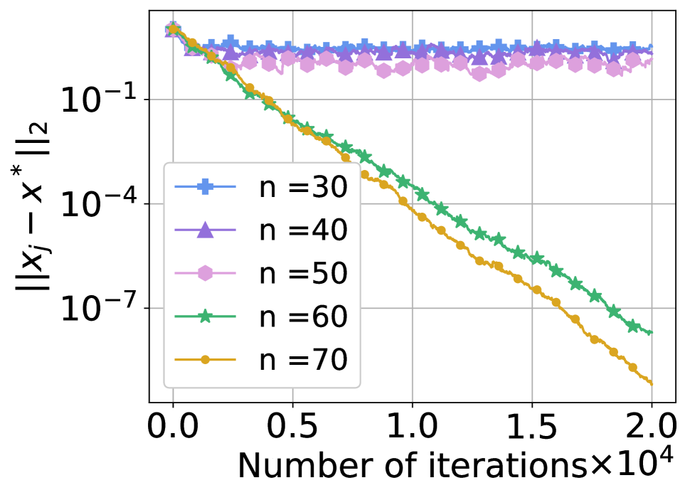
(a) $p=0.8$, without block-list

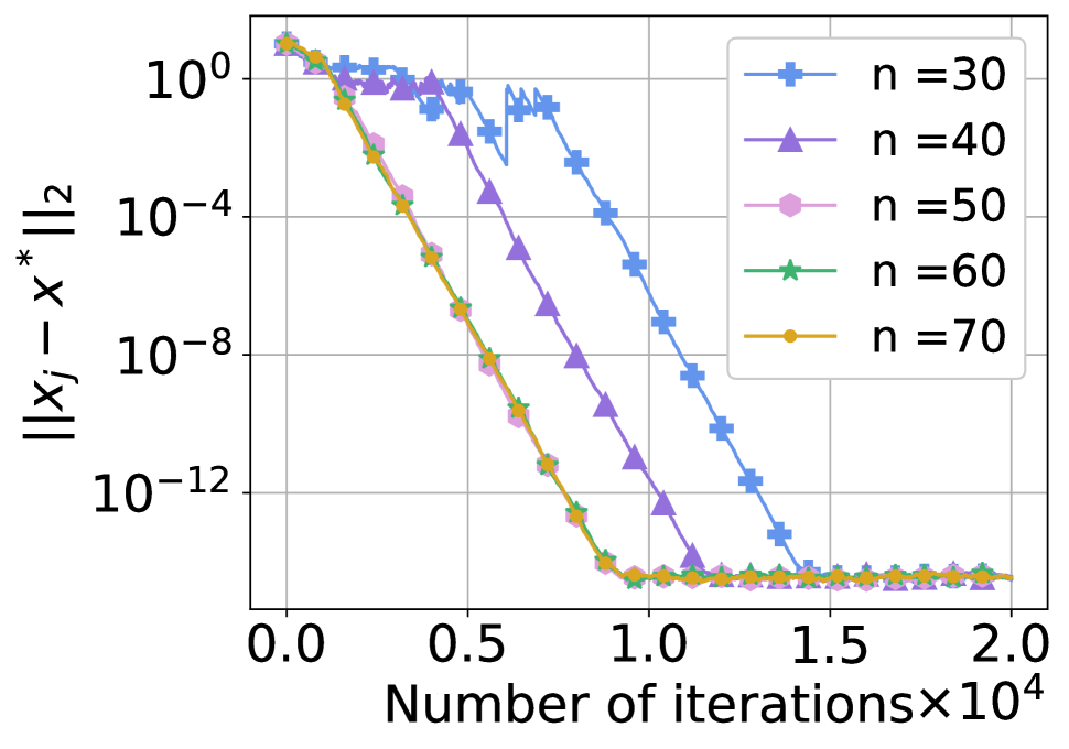
(b) $p=0.8$, with block-list

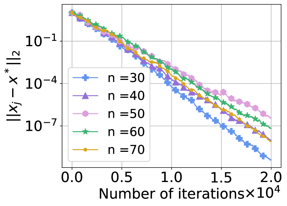
(c) $p=0.2$, without block-list

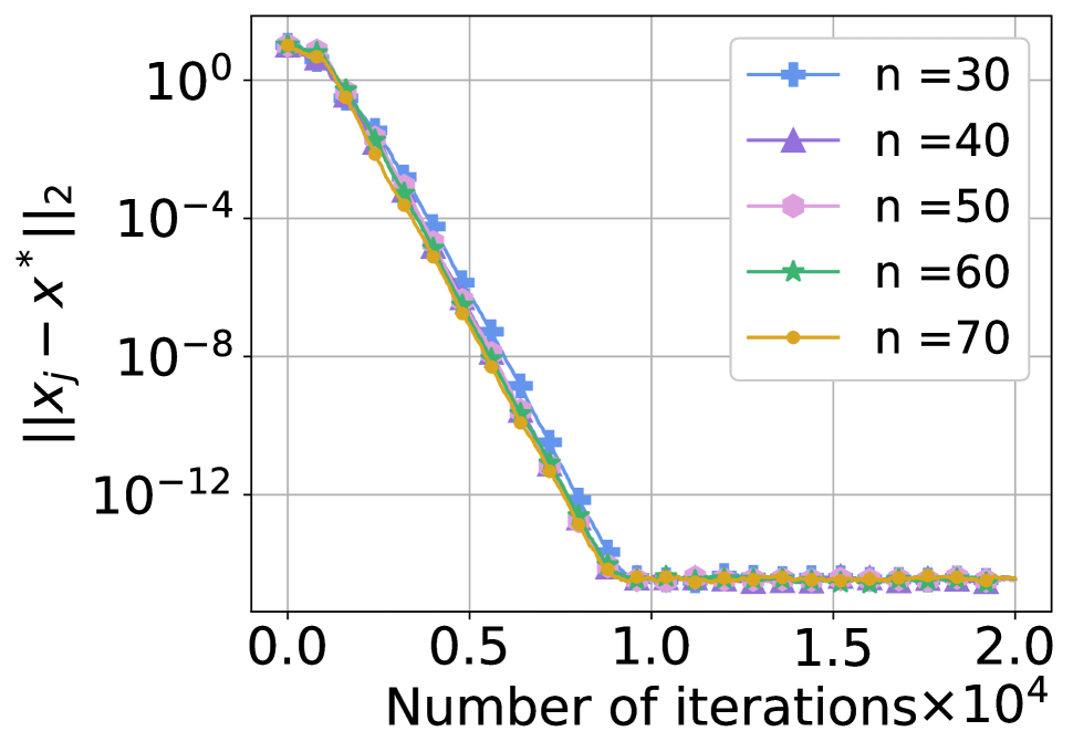
(d) $p=0.2$, with block-list

Fig. 1: The effect of the number of the chosen workers: $10$ error categories and choosing $n$ workers from $100$ workers with $n=30,40,50,60,70$.

In this section, we test the performance of our approach for solving consistent/inconsistent linear systems. The simulation shows how the number of the chosen workers, the adversary rate and the number of the error categories affect the performance.

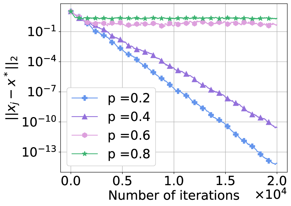
(a) Without block-list

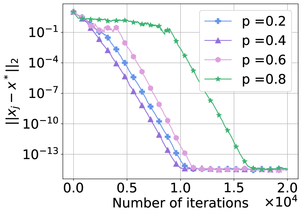
(b) With block-list

Fig. 2: The effect of the adversary rate: $10$ error categories and choosing $10$ workers from $100$ workers.

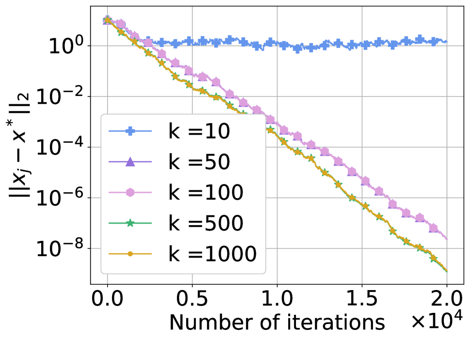
(a) Without block-list

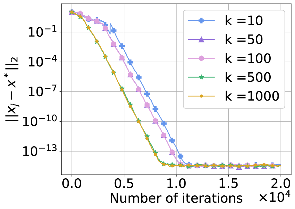
(b) With block-list

Fig. 3: The effect of the error category number: the adversary rate $p=0.8$ and choosing $10$ workers from $100$.

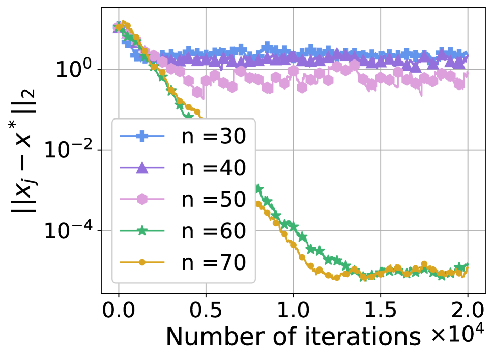
(a) Without block-list

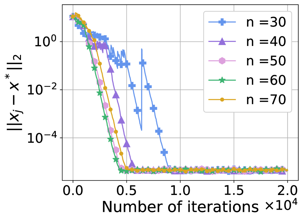
(b) With block-list

Fig. 4: The effect of the number of chosen workers $n$ for inconsistent linear systems: $Ax=b+e$ with random noise $e\sim\text{uniform}(10^{-4})$, adversary rate $p=0.8$, $10$ error categories, and choosing $n$ workers from $100$ with $n=30,40,50,60,70$.

In the simulation, we randomly generate a row-normalized matrix $A\in\mathbb{R}^{m\times n}$, $x\in\mathbb{R}^{n}$ and set $b=Ax$. $Ax=b$ is solved via Alg. 2 with/without block-list. At each iteration, one row of $A$ is randomly chosen and distributed to all chosen workers. Fig. 1 presents the effect of the number of the chosen workers $n$ and shows the convergence results for the mode detection method without/with the block-list, respectively. When the adversary rate $p$ is $20\%$ and $80\%$ over $100$ workers. Without using the block-list method, the central server would use a corrupted step size to update and oscillate around the solution, as shown in Fig. 1(a). When $p=20\%$, the error is as low as $10^{-10}$, although the result is not as good as the one with the block-list, the trade-off is the extra storage for the block-list. As the number of chosen workers $n$ increase from $30$ to $70$ the convergence is faster for both without or with the block-list. The algorithm shows good performance for solving inconsistent linear systems (by adding some random noise to $b$) as well (see Fig. 4). Fig. 2 presents the effect of the adversary rate. As the adversary rate $p$ increases, the accuracy decreases. Even though the adversary rate is large, the final results are still satisfying by solving the system via the algorithm with a block-list. In additional, Fig. 3 shows the effect of the number of category types $k$. The algorithm converges as $k\rightarrow\infty$, i.e. with random noises. With the block-list, the convergence error is less than $10^{-13}$ after a sufficient number of iterations. Furthermore, we summarize performance using precision and recall scores in Table 4. With adequate workers, the algorithm is able to identify the adversaries with an accuracy over $98\%$ and demonstrates the effectiveness of block-list method.

$n$	$30$	$40$	$50$	$60$	$70$
Precision	$0.988$	$0.988$	$1$	$0.988$	$1$
Recall	$0.988$	$0.988$	$1$	$0.988$	$1$

Table 4: Precision and recall of the block-list method when number of used workers $n=30,40,50,60,70$ and adversary rate $p=80\%$.

5 Conclusion

It is of great significant for optimization algorithms to be robust and resistant to adversary. We propose efficient algorithms and provide theoretical convergence guarantee in the presence of the adversarial workers. Our algorithm is able to deal with different adversarial rates even when $p>0.5$, and at the same time, identify the adversarial source. We also present the effect of several important parameters of the adversaries and of the anti-adversaries strategy, namely, the number of error categories $k$, the adversary rate $p$, and the number of chosen workers $n$ at each iteration.

References

- Alistarh et al. (2018) Dan Alistarh, Zeyuan Allen-Zhu, and Jerry Li. Byzantine stochastic gradient descent. arXiv preprint arXiv:1803.08917, 2018.
- Bitar et al. (2020) Rawad Bitar, Mary Wootters, and Salim El Rouayheb. Stochastic gradient coding for straggler mitigation in distributed learning. IEEE Journal on Selected Areas in Information Theory, 2020.
- Gordon et al. (1970) Richard Gordon, Robert Bender, and Gabor T. Herman. Algebraic reconstruction techniques (art) for three-dimensional electron microscopy and x-ray photography. Journal of Theoretical Biology, 29(3):471–481, 1970.
- Gordon et al. (1975) Richard Gordon, Gabor T Herman, and Steven A Johnson. Image reconstruction from projections. Scientific American, 233(4):56–71, 1975.
- Herman and Meyer (1993) Gabor T Herman and Lorraine B Meyer. Algebraic reconstruction techniques can be made computationally efficient (positron emission tomography application). IEEE transactions on medical imaging, 12(3):600–609, 1993.
- Kaczmarz (1937) S Kaczmarz. Angenaherte auflosung von systemen linearer glei-chungen. Bull. Int. Acad. Pol. Sic. Let., Cl. Sci. Math. Nat., pages 355–357, 1937.
- Karakus et al. (2017) Can Karakus, Yifan Sun, Suhas Diggavi, and Wotao Yin. Straggler mitigation in distributed optimization through data encoding. In Advances in Neural Information Processing Systems, pages 5434–5442, 2017.
- Natterer (2001) Frank Natterer. The mathematics of computerized tomography. SIAM, 2001.
- Needell (2009) Deanna Needell. Randomized Kaczmarz solver for noisy linear systems. BIT Numerical Mathematics, 50:395–403, 2009.
- Strohmer and Vershynin (2009) Thomas Strohmer and Roman Vershynin. A randomized kaczmarz algorithm with exponential convergence. Journal of Fourier Analysis and Applications, 15(2):262, 2009.
- Yang and Bajwa (2019) Zhixiong Yang and Waheed U Bajwa. Byrdie: Byzantine-resilient distributed coordinate descent for decentralized learning. IEEE Transactions on Signal and Information Processing over Networks, 5(4):611–627, 2019.