Chan, Huang, and Sarhangian

Dynamic Control of Service Systems with Returns

Dynamic Control of Service Systems with Returns: Application to Design of Post-Discharge Hospital Readmission Prevention Programs

Timothy C. Y. Chan, Simon Y. Huang, Vahid Sarhangian Department of Mechanical and Industrial Engineering, University of Toronto, Toronto ON CANADA tcychan@mie.utoronto.ca, syx.huang@mail.utoronto.ca, sarhangian@mie.utoronto.ca

We study a control problem for queueing systems where customers may return for additional episodes of service after their initial service completion. At each service completion epoch, the decision maker can choose to reduce the probability of return for the departing customer but at a cost that is convex increasing in the amount of reduction in the return probability. Other costs are incurred as customers wait in the queue and every time they return for service. Our primary motivation comes from post-discharge Quality Improvement (QI) interventions (e.g., follow up phone-calls, outpatient appointments) frequently used in a variety of healthcare settings to reduce unplanned hospital readmissions. Our objective is to understand how the cost of interventions should be balanced with the reductions in congestion and service costs. To this end, we consider a fluid approximation of the queueing system and characterize the structure of optimal long-run average and bias-optimal transient control policies for the fluid model. Our structural results motivate the design of intuitive surge protocols whereby different intensities of interventions (corresponding to different levels of reduction in the return probability) are provided based on the congestion in the system. Through extensive simulation experiments, we study the performance of the fluid policy for the stochastic system and identify parameter regimes where it leads to significant cost savings compared to a fixed long-run average optimal policy that ignores holding costs and a simple policy that uses the highest level of intervention whenever the queue is non-empty. In particular, we find that in a parameter regime relevant to our motivating application, dynamically adjusting the intensity of interventions could result in up to 25.4% reduction in long-run average cost and 33.7% in finite-horizon costs compared to the simple aggressive policy. Erlang-R queue; stochastic control; fluid control; bias-optimality, hospital readmission

1 Introduction

We propose and study a control problem for queueing systems where customers may return for additional episodes of service after their initial service completion. The probability of return for each customer can be reduced through what we refer to as a post-service intervention. Post-service interventions are costly but also lead to future savings through eliminating the cost of service for some returning customers, as well as reducing system congestion. Our objective is to understand how the cost of providing post-service interventions should be balanced with the reductions in congestion and service costs.

Our primary motivation comes from Quality Improvement (QI) interventions designed to prevent unplanned hospital readmissions in a variety of healthcare settings. Hospital readmissions are costly and in many cases preventable. QI interventions provided after discharge range from comprehensive transitional care programs (Stauffer et al. 2011) to multi-tier post-discharge follow-up phone calls for pharmaceutical reconciliations (Ravn-Nielsen et al. 2018). Systematic reviews in the medical literature suggest that QI interventions can be effective in reducing readmission risk, although to varying degrees (Leppin et al. 2014). These programs are costly, however, raising the question of whether they are economical for the hospital or more broadly the healthcare system. Findings from economic evaluation studies in the literature range from significant savings to major losses with a systematic review of 21 randomized trials pointing to an overall net loss (Nuckols et al. 2017). The interventions considered in the literature are not usually “optimized” for cost-effectiveness. More importantly, they do not consider the operational benefits of reduced congestion, and only compare the program cost versus the savings in reduced readmission costs. Intuitively, reducing readmission could reduce congestion at hospitals where capacity strain is a common and growing concern. Nevertheless, given the indirect nature of control (only reducing the risk of readmission) and the relatively long time-scale over which readmissions are defined (usually 30 days), the benefits are not clear a priori.

While our models and analysis are primarily motivated by the above healthcare application, they are also relevant to other service systems where returns are undesirable and possibly preventable through post-service interventions. For instance, in the case of overcrowded prisons (see, e.g., Usta and Wein 2015) returns correspond to recidivism and post-service interventions correspond to post-incarceration services and resources (e.g., training, education, and healthcare) aimed at reducing the risk of recidivism; see Wallace (2015) and Badaracco et al. (2021) for examples.

We study the trade-off between the costs of interventions versus the savings in service and holding costs by introducing a control problem for a multiserver queueing system with returns. At each service completion epoch, the decision maker can choose to reduce the probability of return for the departing customer within a closed interval and at a cost that is convex increasing in the amount of reduction in the return probability. That is, in addition to deciding whether to provide the post-service intervention, the decision maker can also adjust the intensity of the intervention. Other costs are incurred as customers wait in the queue and every time they return for service. We are interested in both long-run average cost as well as the transient cost of the system initiated from a congested state. The latter is particularly relevant to healthcare systems, which often experience highly transient dynamics (e.g., due to pandemics, flu season, mass casualty incidents, or regular stochastic fluctuations), and allows us to investigate how the intensity of post-discharge interventions should be adjusted in response to varying levels of congestion in the system.

Queueing systems with returns, also known as Erlang-R, have been studied in the literature, e.g., in support of healthcare staffing decisions (Yom-Tov and Mandelbaum 2014) and to understand the consequences of speed up (i.e., increased service rate) when it leads to higher probability of return (Chan et al. 2014). Dynamic control of the return probability, which is the focus of this paper, has not been studied before. In its most basic form, the Erlang-R queue is a two-node Jackson network where upon service completion at a multiserver node, each customer joins an infinite server node with a certain probability and returns to the first node after some delay in the second node. From a technical standpoint, the problem of controlling the return probability is challenging since the transition rates of the underlying Markov process are unbounded. This prevents one from applying the typical approach of exploiting a uniformized Markov Decision Process (MDP). Although some methods have been proposed in the literature to address this issue (e.g., in Down et al. 2011, Bhulai et al. 2014, and Zayas-Cabán et al. 2016) they exploit specific structures of their respective problems, which are hard to generalize and do not apply to our setting. In contrast, we rely on analysis of associated fluid control problems which provide structural insights and practical policies.

Our main results and contributions can be summarized as follows.

Queueing model with controllable return probability: We propose and study a new control problem for the Erlang-R queue, with the key feature that the return probability can be controlled at departure instances. Reducing the return probability incurs a cost that is convex increasing in the amount of reduction. The model captures a tradeoff between the cost of post-service intervention and the savings in holding and return costs.

Long-run average control: We show that when the fluid model is stable without any intervention (i.e., under the maximum return probability) a fixed return probability, which we refer to as the equilibrium policy, minimizes its long-run average cost. In equilibrium the queue is empty and the optimal return probability balances the cost of intervention versus cost of return incurred in equilibrium. This, however, ignores any holding costs incurred starting from an initial condition far from the equilibrium.

Bias-optimal transient control: To minimize the transient cost incurred before reaching the equilibrium, we propose and study a fluid control problem that seeks bias-optimality, i.e., minimizes the cost difference with that of the equilibrium policy over an infinite horizon. We show that the infinite-horizon problem is well-defined and is equivalent to a finite-horizon problem that is easier to analyze. We then characterize the structure of the optimal transient policy by exploiting Pontryagin’s Minimum Principle. In particular, we show that for states where the queue is non-empty, the optimal policy under a general convex intervention cost is characterized by a set of straight contour lines in the state space. Points on each line are equivalent with respect to a certain measure of congestion comprised of the number of customers currently in the system, as well as a discounted count of those waiting to return. When the cost is piecewise linear with $k$ pieces, $k$ lines “fan out” in the state space, dividing it into regions with the same optimal probability of return. This simple structure is practically appealing since it motivates the design of “surge protocols” whereby different levels of the post-service intervention are offered depending on the congestion level of the system. We further discuss and illustrate the relevance of our results to systems with time-varying arrivals both analytically and numerically.

Numerical results: Through extensive simulation experiments, we evaluate the performance of the fluid policy for the stochastic system over both finite and infinite horizons, and in comparison with two benchmark polices: the equilibrium policy which ignores congestion, and a simple policy which always uses the highest level of intervention when all servers are busy. We find that by accounting for holding cost reductions, interventions that may otherwise not be economical could lead to significant cost savings, in particular when the cost of intervention is relatively high. As the holding cost increases, the performance of the fluid policy approaches that of the simple policy. However, in a relevant parameter regime, with high intervention cost and moderate holding cost, dynamically adjusting the intensity of the interventions in response to congestion could result in up to 25.4% reduction in long-run average cost and 33.7% in finite-horizon costs compared to the simple policy. Finally, we conduct a case study where we relax some of our modeling assumptions and calibrate the inputs of our model based on efficacy and economic data for a real post-discharge intervention designed for reducing readmission of heart failure patients. The results illustrate the robustness of our qualitative observations to certain modelling assumptions for practically relevant parameters.

The rest of this paper is organized as follows. We conclude this section with a brief review of the related literature. In Section 2 we describe the queueing model and its fluid approximation. We formulate and analyze the associated fluid control problems for long-run average control in Section 3 and for transient control in Section 4. We discuss the extension and robustness of our results to time-varying arrivals in Section 5. Section 6 summarizes the results of our numerical experiments and case study. We conclude the paper in Section 7. All proofs are presented in the E-Companion.

1.1 Related Literature

From a modeling perspective our work is related to previous studies of the Erlang-R queue. Yom-Tov and Mandelbaum (2014) proposes and studies the Erlang-R queue under time-varying arrival rates in support of various healthcare staffing problems, including bed capacity planning in wards with readmission, physician staffing in the emergency department, and provider staffing for a mass casualty incident. Several studies have investigated the performance and stability of the Erlang-R model under state-dependent service and return probabilities. Chan et al. (2014) considers a threshold speedup policy where if the queue length exceeds a fixed threshold, the service rate increases to clear the congestion but at the cost of the return probability also increasing. They utilize a fluid approximation of the model and investigate its stability. Ingolfsson et al. (2020) compare the equilibrium and transient behavior of two fluid models for a system with state-dependent service and return probabilities, differing in terms of when the determination of whether a customer will return to service is made. Barjesteh and Abouee-Mehrizi (2021) study a more general multiclass model where the service rates depend on the workload of the system and the return probabilities on the service rate and investigate the criteria for stability of the system. In contrast to these previous studies which focus on stability and performance analysis, our work is concerned with the dynamic control of the return probabilities at departure instances.

From a methodological perspective, our work relates to the vast literature on queueing control and specifically studies concerned with transient control. Analysis of transient dynamics is typically challenging even under a given control policy. Fluid models approximately capture the transient dynamics of the system, and as such associated fluid control problems have been used in a variety of queueing models to gain insights on the structure of “good” policies, especially for scheduling and routing problems, e.g., Avram et al. (1994), Perry and Whitt (2009), Larranaga et al. (2013), and Hu et al. (2021). For certain fluid control problems, the total cost over an infinite horizon remains finite under appropriate stability conditions, allowing one to obtain stationary optimal policies. This is typically the case for control problems concerned with single-server queues, e.g., a class of scheduling problems studied in Maglaras (2000) and a multiclass revenue maximization problem considered in Maglaras (2006), but can also (depending on the cost structure) hold for multiserver problems, e.g., as in Chan et al. (2021). When costs are also incurred in equilibrium, as in the case of our problem, the infinite horizon cost diverges and hence is not suitable for analysis. Alternatively, one can consider minimizing the total cost until reaching a certain state, e.g., as in Ata and Peng (2020) and Hu et al. (2021), which leads to a control problem with state-dependent constraints. For our multiserver problem, the equilibrium is reached asymptotically as time tends to infinity. As such, we instead consider bias-optimal policies. The idea is related to the concept of bias-optimality in MDPs, where a bias-optimal policy is one that minimizes the relative value function among all policies that are long-run average optimal; see, e.g., Lewis and Puterman (2002) for a review and Haviv and Puterman (1998) for an application to an admission control problem. Larrañaga et al. (2015) also study a bias-optimal fluid control problem, but to derive approximate index policies for a multiclass scheduling problem with abandonment. As such, their problem and approach differ from ours.

With respect to our main motivating application, our work relates to studies aiming to evaluate or propose economical and/or operational interventions to reduce hospital readmissions, see, e.g., Zhang et al. (2016), Arifoğlu et al. (2021) and Shi et al. (2021) among others. More closely related are studies concerned with post-discharge interventions. Bayati et al. (2014) proposes targeting interventions to high-risk patients as identified using a predictive model. Helm et al. (2016) propose a model to optimize the type and timing of checkups to implement post-discharge monitoring plans. Liu et al. (2018) combines a prediction model with a deterministic optimization model to optimize a post-discharge monitoring schedule and staffing plan to support monitoring patients before they end up readmitting. These studies, however, do not consider the potential benefits of reduced congestion at the hospital. In contrast, we focus on understanding how the post-discharge intervention plans help reduce congestion.

2 Model Description

We consider a multiserver queueing network with returns, also known as the Erlang-R model (Yom-Tov and Mandelbaum 2014). New customers arrive to the system according to a Poisson process with rate $\lambda$ and have exponentially distributed service requirements with rate $\mu$. There are $N$ identical servers available. If all servers are busy, customers wait in an infinite capacity queue. Upon completing service, and in the absence of a post-service intervention, a customer leaves the system with probability $1-p_{u}$, and returns to the system after an exponentially distributed time with rate $\nu$ with probability $p_{u}$. Let $\{X(t);t\geq 0\}$ denote the process that keeps track of the number of customers currently in the system (i.e., in service or waiting), and let $\{Y(t);t\geq 0\}$ denote the process that keeps track of the number of customers whose return to the system is pending. Following Véricourt and Jennings (2011) and Yom-Tov and Mandelbaum (2014), we refer to the customers currently in the system as Needy and those who will return at a later time as Content.

The system incurs costs as customers wait, return, and undergo post-service interventions. Needy customers incur a holding cost at rate $h$ as they wait in the queue. For each returning customer, the system incurs a fixed return cost of $r$. Upon service completion, the decision maker has the option of implementing a post-service intervention that can reduce the probability of return for the departing customer. More specifically, we assume that the decision maker can directly control the return probability in the interval $[p_{l},p_{u}]$ where $0<p_{l}<p_{u}<1$. The intervention cost of setting the return probability to $p\in[p_{l},p_{u}]$ is denoted by $C(p)$.

The intervention cost function $C(\cdot)$ is convex, non-negative, decreasing, and continuously differentiable with $C(p_{u})=0$.

We consider the set of Markovian policies under which the probability of return is determined based on the state of the system at departure instances of Needy customers. Denote by $p^{\pi}(x,y)$ the probability of return for a Needy customer departing the system at state $(X(t),Y(t))=(x,y)$ under intervention policy $\pi$. Since the dynamics of the process $\{(X(t),Y(t));t\geq 0\}$ depends on the intervention policy we denote the process under policy $\pi$ by $\{(X^{\pi}(t),Y^{\pi}(t);t\geq 0\}$. Further, denote by $\{R^{\pi}(t);t\geq 0\}$ the process that keeps track of the cumulative number of returns under policy $\pi$, and by $\{D^{\pi}(t);t\geq 0\}$ the process that keeps track of the cumulative number of departures from the Needy state. Finally, let $\{t_{1},t_{2},\ldots\}$ denote the decision epochs, i.e., the sequence of instances when Needy customers depart the system. The expected total cost over the finite horizon of $[0,T]$ and starting from $(X(0),Y(0))$ can be expressed as,

$$\mathcal{G}^{\pi}(T)=\mathbb{E}\left[\int_{0}^{T}h(X^{\pi}(t)-N)^{+}dt+rR^{\pi}(T)+\sum_{i=1}^{D^{\pi}(T)}C\left(p^{\pi}\left(X^{\pi}(t_{i}),Y^{\pi}(t_{i})\right)\right)\right],$$ (1)

where $(x)^{+}\equiv\max(x,0)$. This cost function is composed of three terms, representing the holding, return, and intervention costs, respectively, over the time horizon $[0,T]$.

It is natural to consider finding policies that minimize the long-run average cost of the system, that is,

$$\limsup_{T\to\infty}\frac{1}{T}\mathcal{G}^{\pi}(T).$$ (2)

However, if the initial state of the system is far from its steady-state, a long-run average policy could be sub-optimal in the short-term as it ignores the initial transient costs incurred in the system. As such, one may consider searching for a policy that minimizes the finite-horizon cost in (1) over an appropriate horizon-length. Due to the complexity of the stochastic control problem, we consider a fluid approximation of the queueing model and formulate associated (deterministic) fluid control problems. The fluid control problem yields approximately optimal policies for the stochastic problem, and provides insights on the structure of optimal policies.

2.1 The Fluid Model

The fluid model is obtained by replacing the stochastic arrival, service, and return processes by their deterministic average rates. Denote by $(x(t),y(t))$ the state of the fluid model at time $t\geq 0$ where $x(t)$ and $y(t)$ are the amount of Needy and Content fluid (customers), respectively, in the system at time $t$. Under an intervention policy $\pi$, the fluid dynamics satisfy the following system of ordinary differential equations (ODEs):

$$\dot{x}(t) =\lambda+\nu y(t)-\mu(x(t)\wedge N),$$ (3)

$$\dot{y}(t) =-\nu y(t)+\mu p^{\pi}(x(t),y(t))(x(t)\wedge N),$$ (4)

where $x(t)\wedge N\equiv\min(x(t),N)$ is the number of busy servers at time $t$. The instantaneous rate of change for the fluid trajectories in (3)–(4) is composed of an input and output rate. In (3), the input rates correspond to the arrival of new and returning customers, whereas the output rate corresponds to service completions of Needy customers. In (4), the input is the fraction of departing Needy customers who join the Content state, and the output rate is the rate at which current Content customers transition into the Needy state.

The fluid approximation is formally justified as a Functional Strong Law of Large Numbers (FSLLN) for the stochastic processes described in Section 2. It is obtained by considering a sequence of stochastic systems in which the arrival rates, number of servers, and the initial conditions grow linearly, while the service and return rates remain unscaled. Assuming that $p^{\pi}(\cdot,\cdot)$ is Lipschitz, Theorem 2.2. of Mandelbaum et al. (1998) implies that the sequence of fluid-scaled processes converge, almost surely and uniformly on compact sets, to deterministic and absolutely continuous trajectories $(x(t),y(t))$ satisfying (3)–(4).

To ensure stability, in our analysis of the associated fluid control problems we impose the following assumption on the parameters.

The maximum return probability satisfies $p_{u}<1-\lambda/(\mu N)$. As shown in Chan et al. (2014) for the Erlang-R fluid model with a fixed return probability $p$, if $p<1-\lambda/(\mu N)$, then starting from any initial condition the trajectories converges to the following globally stable equilibrium,

$$(x_{\infty},y_{\infty})=\left(\frac{\lambda}{\mu(1-p)},\frac{\lambda p}{\nu(1-p)}\right),$$ (5)

and diverge otherwise. Hence, Assumption 2.1 guarantees that in the absence of intervention (i.e., with constant return probability $p_{u}$) the fluid model remains stable.

3 Long-Run Average Control

In this section, we formulate the long-run average fluid control problem and characterize the structure of an optimal policy. We assume that fluid waiting in queue incurs a holding cost at rate $h$, returning fluid incurs a cost at rate $r$, and that departing fluid at time $t$ incurs an intervention cost at rate $C(p(t))$. Starting from a given initial condition $(x^{0},y^{0})$, the problem is to find an admissible intervention policy $p(\cdot)$ that minimizes the long-run average cost:

$$\min_{p(\cdot)\in{\mathcal{P}}}\>\limsup_{T\to\infty}\>\frac{1}{T}\int_{0}^{T}\left(h(x(t)-N)^{+}+r\nu y(t)+C(p(t))\mu(x(t)\wedge N)\right)\,dt.$$ (6)

The set ${\mathcal{P}}$ defines the set of admissible policies. A policy $p(\cdot)\in{\mathcal{P}}$ is admissible if it jointly satisfies,

$$\dot{x}(t)=\lambda+\nu y(t)-\mu(x(t)\wedge N),\quad\forall\,t\in[0,T],$$ (7)

$$\dot{y}(t)=-\nu y(t)+\mu p(t)(x(t)\wedge N),\quad\forall\,t\in[0,T],$$ (8)

$$p(t)\in[p_{l},p_{u}],\quad\forall\,t\in[0,T],$$ (9)

$$(x(0),y(0))=(x^{0},y^{0}),$$ (10)

with an absolutely continuous $(x(t),y(t))$. Before turning into the analysis of the control problem, we partition the state space ${\mathbb{R}}^{2}_{+}$ into three regions: $(i)$ ${\mathcal{C}}:=(N,\infty)\times[0,\infty)$; $(ii)$ ${\mathcal{A}}:=[0,N]\times[0,\frac{\mu N-\lambda}{\nu}]$; and $(iii)$ ${\mathcal{N}}:=[0,N]\times(\frac{\mu N-\lambda}{\nu},\infty)$. We refer to ${\mathcal{C}}$ as the congested region since it represents states where all servers are busy and the queue is non-empty. In contrast, ${\mathcal{N}}$ and ${\mathcal{C}}$ represent states where the queue is empty. Figure 1 provides an illustration of the three regions.

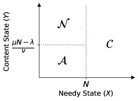
Figure 1: An illustration of the three partitions of the state space.

Our first result establishes that the trajectories must reach the corner region ${\mathcal{A}}$ within a bounded time and then remain there thereafter.

Proposition 3.1

$(i)$ For any given initial state $(x^{0},y^{0})\geq 0$, there exists a time $t_{{\mathcal{A}}}<\infty$ such that $x(t_{\mathcal{A}}),y(t_{\mathcal{A}}))\in{\mathcal{A}}$ under any admissible policy $p(\cdot)\in{\mathcal{P}}$. $(ii)$ If $(x^{0},y^{0})\in{\mathcal{A}}$, then $(x(t),y(t))\in{\mathcal{A}}$ for all $t\geq 0$.

The proposition states that region ${\mathcal{A}}$ is absorbing under any admissible policy: all trajectories are guaranteed to reach ${\mathcal{A}}$ within a common time bound, and once they reach ${\mathcal{A}}$, they remain in ${\mathcal{A}}$ thereafter. Since the queue is empty in ${\mathcal{A}}$, we have $(x(t)-N)^{+}=0$ and $x(t)\wedge N=x(t)$ for $t\geq t_{{\mathcal{A}}}$. Hence, when considering long-run average performance we may replace the objective in (6) with

$$\min_{p(\cdot)\in{\mathcal{P}}}\>\limsup_{T\to\infty}\>\frac{1}{T}\int_{0}^{T}r\nu y(t)+C(p(t))\mu x(t)\,dt.\\$$ (11)

3.1 Optimizing Amongst Equilibria

If we restrict our attention to policies that result in convergence to an equilibrium point in the form of (5), minimizing the long-run average cost is equivalent to finding a fixed policy $p_{\infty}\in\argmin_{p}J(p)$, where

$$J(p):=\lambda\frac{rp+C(p)}{1-p}.$$ (12)

We may interpret $J(p)$ as the long-run average cost rate under a constant policy $p(t)=p$ for all $t\geq 0$: the total arrival rate (including returns) is $\lambda/(1-p)$ and each arrival incurs an intervention cost of $C(p)$, while a fraction $p$ of the arrivals incur a return cost of $r$. Further, since in the long-run the queue is empty, no congestion cost is incurred. We will show in Proposition 4.3 that $J_{\infty}:=J(p_{\infty})$ is indeed the optimal long-run average cost and hence focusing on policies under which the trajectories converge to an equilibrium is not restrictive.

Our next result characterizes the structure of the equilibrium cost rate $J(\cdot)$ which, depending on the parameters, may be convex, concave, or neither. However, it is minimized at all of its critical points, or at an endpoint if no critical points exist.

Proposition 3.2

$J(\cdot)$ is unimodal. Further, its minimizer(s) can be characterized as follows:

1. If $(1-p_{l})C^{\prime}(p_{l})+C(p_{l})+r\geq 0$, then $J(\cdot)$ is non-decreasing and hence minimized at $p_{l}$.

2. If $(1-p_{u})C^{\prime}(p_{u})+C(p_{u})+r\leq 0$, then $J(\cdot)$ is non-increasing and hence minimized at $p_{u}$.

3. Otherwise, $J(\cdot)$ has at least one critical point, and its critical points form a closed interval. If this interval has positive length, then they are all minimizers of $J(\cdot)$, and $C(\cdot)$ is linear along this interval.

The result is intuitive. If the intervention is “cheap enough”, it is optimal to provide the highest level of intervention and reduce the return probability to its minimum $p_{l}$, and if it is “too costly” it is optimal to not provide any intervention and maintain the return probability at $p_{u}$. Otherwise, the optimal return probability takes a value between the two extreme values. In this case, $J(\cdot)$ is roughly U-shaped: it decreases for small $p$ near $p_{l}$, then attains its minimum, and finally increases for large $p$ near $p_{u}$. While the minimum is not guaranteed to be unique, the minimizing values are contiguous, forming a closed interval. Any constant policy lying in this interval will yield the minimum long-run average cost.

The following corollary specializes the result to the case of a linear intervention cost and follows directly from Proposition 3.2. For brevity, we omit the proof.

Corollary 3.3

If $C(\cdot)$ is linear, then one of the following two cases holds:

1. If $r(p_{u}-p_{l})/(1-p_{u})\leq C(p_{l})-C(p_{u})$, then $J(\cdot)$ is minimized at $p_{l}$.

2. If $r(p_{u}-p_{l})/(1-p_{u})\geq C(p_{l})-C(p_{u})$, then $J(\cdot)$ is minimized at $p_{u}$.

Under a linear intervention cost, the optimal return probability is one of the two extreme points of the interval. The condition required for either of the two extreme points to be optimal is intuitive. Under a constant return probability of $p_{u}$, we incur a total of $rp_{u}/(1-p_{u})$ in readmission costs per patient. If we treat $p_{u}$ as the baseline policy, the quantity $r(p_{u}-p_{l})/(1-p_{u})$ is the reduction in lifetime readmission costs (i.e., considering future returns) that can be achieved via a one-time intervention that reduces the customer’s return probability to $p_{l}$ at their first service completion. This quantity is evaluated against $C(p_{l})-C(p_{u})$, i.e., the cost of providing such an intervention.

4 Transient Control

Under the long-run average cost objective, any policy that eventually enforces an optimal fixed return probability is optimal, even though it may be “wasteful” in the initial transient period. In particular, starting from an initial state far from the equilibrium, we may incur significant holding costs in the queue, which are ignored under a fixed optimal long-run average policy. In this section, we obtain policies that also minimize the transient cost incurred before reaching the equilibrium.

We begin by formulating the transient control problem and presenting some preliminary results in Section 4.1. We next investigate the structure of optimal transient policies starting with a non-empty queue in Section 4.2 and starting with an empty queue in Section 4.3. Finally, we illustrate the results using numerical examples in Section 4.4.

4.1 Formulation of the Associated Fluid Control Problem and Preliminaries

We consider a problem that seeks bias-optimality, i.e., minimizing the total cost incurred above/below the long-run average cost $J_{\infty}$:

$$\min_{p(\cdot)\in{\mathcal{P}}}\ \int_{0}^{\infty}\left(h(x(t)-N)^{+}+r\nu y(t)+C(p(t))\mu(x(t)\wedge N)-J_{\infty}\right)\,dt,$$ (13)

where an admissible policy $p(\cdot)\in{\mathcal{P}}$ must satisfy $\eqref{eq:fluid_C1}$–(10) over an infinite horizon. In the following, we show that this problem is well-defined, i.e., it has a finite optimal cost despite being undiscounted. We also establish its equivalence to a finite-horizon problem that is easier to analyze and confirm that $J_{\infty}$ is indeed the minimum long-run average cost.

We first define the finite-horizon control problem as,

$$\min_{p(\cdot)\in{\mathcal{P}}}\ \int_{0}^{T}\left(h(x(t)-N)^{+}+r\nu y(t)+C(p(t))\mu(x(t)\wedge N)-J_{\infty}\right)\,dt+\Psi(x(T),y(T)),$$ (14)

where

$$\Psi(x,y)=\frac{(rp_{\infty}+C(p_{\infty}))x+(r+C(p_{\infty}))y}{1-p_{\infty}}.$$ (15)

Observe that the state at time $T$ is assigned the terminal cost $\Psi$, which charges a penalty for each Needy and Content customer in the system at time $T$. This penalty can be interpreted as the future cost of each customer (ignoring congestion), assuming that a constant policy of $p(t)=p_{\infty}$ is enforced for $t\geq T$. For each Content customer in the system, the penalty includes the return cost $r$ plus the intervention cost $C(p_{\infty})$, with each subsequent return incurring the same costs. As the fraction of returning customers equals $p_{\infty}$, the geometric series summing all the future costs yields $(r+C(p_{\infty}))/(1-p_{\infty})$. Similarly, for Needy customers the penalty includes the intervention cost $C(p_{\infty})$, and the future cost of $(r+C(p_{\infty}))/(1-p_{\infty})$ incurred for a fraction $p_{\infty}$ of customers who transition into the Needy state. Summing together, the future cost of Needy customers is $(rp_{\infty}+C(p_{\infty}))/(1-p_{\infty})$. Note that this value is equal to $J_{\infty}/\lambda$ as new customers arriving at a rate of $\lambda$ together contribute an additional cost of $J_{\infty}$ in equilibrium.

Proposition 4.1

Let $V_{T}(x,y,t)$ denote the optimal cost-to-go of the finite horizon problem in (14) with horizon $T$, starting from state $(x,y)$ at time $t$. If $(x,y)\in{\mathcal{A}}$, then $(i)$ the optimal policy is given by $p(t)=p_{\infty}$ for all $t\geq 0$, and $(ii)$ the value function is given by $V_{T}(x,y,t)=\Psi(x,y)$.

As expected, $p_{\infty}$ is an optimal policy when starting from region ${\mathcal{A}}$. Furthermore, the value function is independent of time and equals the terminal cost function $\Psi$. This suggests an equivalence to the infinite-horizon problem. The following proposition establishes that the infinite-horizon problem is well-defined.

Proposition 4.2

Let $V_{\infty}(x,y)$ denote the optimal cost of the infinite horizon problem in (13) starting from $(x,y)$. Then, $-\infty<V_{\infty}(x,y)<\infty$ for all $(x,y)\in{\mathbb{R}}^{2}_{+}$.

Proposition 4.2 also implies that $J_{\infty}$ is indeed the optimal value of the long-run average problem, since otherwise $V_{\infty}(x,y)$ would be infinite.

Proposition 4.3

$J_{\infty}$ is the optimal long-run average cost over all policies $p(\cdot)\in{\mathcal{P}}$.

It is now easy to verify the equivalence of the infinite-horizon problem in (13) and the finite-horizon problem in (14) for a sufficiently large $T$. For $(x^{0},y^{0})\in{\mathcal{A}}$, Proposition 4.1 implies that the optimal policy of the infinite-horizon problem agrees with that of the finite-horizon problem on $[0,T]$, and the two problems share the same optimal objective value. The terminal value function $\Psi$ used in the finite-horizon formulation is the value function of the infinite-horizon problem (up to an additive constant). To extend the equivalence to all initial states, we may separate the infinite horizon into a transient period (up to a finite horizon $T$) and a tail period. If $T$ is sufficiently large, then by Proposition 3.1 we are guaranteed that $(x(T),y(T))\in{\mathcal{A}}$, and hence the tail part must have cost $\Psi(x(T),y(T))$. As such, we can study these two equivalent problems interchangeably.

4.1.1 Pontryagin’s Minimum Principle.

To study the optimal transient policy, we exploit Pontryagin’s minimum principle for the finite-horizon formulation with a large horizon $T$. To this end, we define the Hamiltonian function as,

$$H(x,y,p,t) :=h(x-N)^{+}+r\nu y+C(p)\mu(x\wedge N)-J_{\infty}+(\lambda+\nu y-\mu(x\wedge N))\gamma_{1}(t)$$

$$\qquad+(-\nu y+\mu p(x\wedge N))\gamma_{2}(t).$$ (16)

The vector $(\gamma_{1},\gamma_{2})$ is referred to as the adjoint, or costate vector, and is analogous to a Lagrange multiplier (see, e.g., Todorov 2006). The costate follows the gradient of the value function along the optimal trajectory. It thus captures the marginal cost of each additional Needy and Content patient at each point in time along the optimal trajectory.

Pontryagin’s minimum principle provides necessary conditions on optimality. Specifically, an optimal policy $p^{*}(t)$ must minimize the Hamiltonian at every time $t$, and the Hamiltonian must always equal zero along an optimal trajectory. That is, for all $t\geq 0$:

$$H(x(t),y(t),p^{*}(t),t) =0,$$ (17)

$$H(x(t),y(t),p^{*}(t),t) =\underset{p\in[p_{l},p_{u}]}{\min}H(x(t),y(t),p,t).$$ (18)

Additionally, the costate vector $(\gamma_{1},\gamma_{2})$ is governed by the following system of ODEs and boundary conditions (see, e.g., Kirk 1998):

$$\dot{\gamma}_{1}(t) =-H_{x}(x(t),y(t),p(t),t),$$ (19)

$$\dot{\gamma}_{2}(t) =-H_{y}(x(t),y(t),p(t),t),$$ (20)

$$\gamma_{1}(T) =\Psi_{x}(x(T),y(T))=\frac{rp_{\infty}+C(p_{\infty})}{1-p_{\infty}},$$ (21)

$$\gamma_{2}(T) =\Psi_{y}(x(T),y(T))=\frac{r+C(p_{\infty})}{1-p_{\infty}}.$$ (22)

The system of ODEs describe the evolution of the trajectories $(x,y)$, $(\gamma_{1},\gamma_{2})$ over time. However, the dynamics differ depending on whether all servers are busy or not. Therefore, we separately analyze the two cases. Before turning to the main analysis, we present the following result which follows directly from the optimality conditions.

Proposition 4.4

Under a linear intervention cost function $C(\cdot)$ the optimal transient policy is a bang-bang control policy.

With a linear intervention cost function, an optimal policy only switches between the two extreme values of $p_{l}$ or $p_{u}$. We further investigate the structure of an optimal transient policy including under a general convex cost function next.

4.2 Optimal Transient Policy Starting with a Non-Empty Queue

In this section, we characterize the structure of the optimal transient policy starting from an initial condition in ${\mathcal{C}}$, i.e., when the system is initiated with a non-empty queue.

From Proposition 3.1 we know that the trajectories eventually reach ${\mathcal{A}}$, regardless of the policy used. Let $\tau:=\inf\{t\geq 0;x(t)=N\}$ denote the time at which the trajectories reach ${\mathcal{A}}$ under an optimal policy. We can then step backwards from $T$ to $\tau$ at which point the costates are at their constant equilibrium values, the Needy state is $x(\tau)=N$, and the Content state $y(\tau)$ is at some value between $0$ and $(\mu N-\lambda)/\nu$. To step further back in time, we switch to solving a different system which captures the dynamics when the queue is non-empty, using these four values as boundary conditions. Finally, we characterize the policy as a function of the state by exploiting the requirement of Pontryagin’s minimum principle that the Hamiltonian must equal zero along the optimal trajectory.

4.2.1 Optimal Policy as a Function of Time.

We begin by solving the system in (19)–(22) to determine the costate trajectories. We present the solution in the following lemma. The proof is straightforward and hence omitted.

Lemma 4.5

$(i)$ For $t\in[\tau,T]$, the costates are constant and given by,

$$\gamma_{1}(t) =\frac{rp_{\infty}+C(p_{\infty})}{1-p_{\infty}},$$ (23)

$$\gamma_{2}(t) =\frac{r+C(p_{\infty})}{1-p_{\infty}}.$$ (24)

$(ii)$ For $t\in[0,\tau)$, the costates are strictly decreasing and are given by:

$$\gamma_{1}(t) =h(\tau-t)+\frac{rp_{\infty}+C(p_{\infty})}{1-p_{\infty}},$$ (25)

$$\gamma_{2}(t) =\frac{h}{\nu}(e^{-\nu(\tau-t)}+\nu(\tau-t)-1)+\frac{r+C(p_{\infty})}{1-p_{\infty}}.$$ (26)

Next, we proceed to characterize the optimal policy $p^{*}(t)$ as a function of time. Pontryagin’s minimum principle states that if a policy $p^{*}(t)$ is optimal, then $p^{*}(t)$ must minimize $H(x(t),y(t),p,t)$ for all $t\geq 0$. In our case, this condition simplifies to requiring that $p^{*}(t)\in\argmin_{p}\phi_{t}(p)$, where $\phi_{t}(p):=C(p)+\gamma_{2}(t)p$. Since $C(\cdot)$ is assumed to be convex and continuously differentiable, the same must hold for $\phi_{t}(\cdot)$. As such, minimization occurs at a critical point, characterized by the first-order condition $C^{\prime}(p)=-\gamma_{2}(t)$, or at an endpoint if no critical points exist.

Proposition 4.6

Any optimal policy must be non-increasing in time during $t\in[0,\tau)$. Specifically, it must be of the form:

$$p^{*}(t)=\begin{cases}p_{u},&\gamma_{2}(t)<-C^{\prime}(p_{u}),\\ p\text{ such that }C^{\prime}(p)=-\gamma_{2}(t),&-C^{\prime}(p_{u})\leq\gamma_{2}(t)\leq-C^{\prime}(p_{l}),\\ p_{l},&\gamma_{2}(t)>-C^{\prime}(p_{l}).\end{cases}$$ (27)

Furthermore, the optimal policy $p^{*}(t)$ is almost everywhere unique on $[0,\tau)$.

An interior return probability $p\in(p_{l},p_{u})$ can only be optimal at an instant where $C^{\prime}(p)=-\gamma_{2}(t)$, since $\gamma_{2}$ is strictly decreasing. If $C^{\prime}(p)=-\gamma_{2}(t)$ for multiple values of $p$, then all such values are optimal. This can happen for at most countably many $t$ and hence policies satisfying (27) must agree almost everywhere (with respect to time). These differences are inconsequential as they do not affect the state trajectory nor the objective value. Therefore, the optimal policy is almost everywhere unique up until time $\tau$.

4.2.2 Optimal Policy as a Function of State.

So far, we have characterized the optimal policy as a function of time and in terms of the value $\tau$. If we know the value of $\tau$ associated with the initial state $(x^{0},y^{0})\in{\mathcal{C}}$ under the optimal policy, we can then simply apply Proposition 4.6 starting from time $t=0$ until we reach ${\mathcal{A}}$, after which we switch to the equilibrium policy. However, the value of $\tau$ is not known, making the result not directly applicable. Instead, suppose that we start with a particular value of $\tau$. Then $p^{*}(0),\gamma_{1}(0)$, and $\gamma_{2}(0)$ can all be computed for this particular $\tau$. The requirement that $H(x^{0},y^{0},p^{*}(0),t)=0$ then becomes a constraint on the corresponding state $(x^{0},y^{0})$. In other words, all states which are exactly $\tau$ time away from ${\mathcal{A}}$ must satisfy what turns out to be a linear constraint, allowing for characterization of the optimal policy as a function of the state. As we discuss below further, this characterization provides structural insights but also allows for the computation of the optimal policy for all states in ${\mathcal{C}}$.

Theorem 4.7

Suppose $(x,y)\in{\mathcal{C}}$. Under the optimal policy, there exists a unique $\tau>0$ such that $(x,y)$ lies on the line:

$$h(x-N)+h(1-e^{-\nu\tau})y-J_{\infty}+(\lambda-\mu N)\gamma_{1}(\tau)+\mu N\left(C(p^{*})+\gamma_{2}(\tau)p^{*}\right)=0,$$ (28)

where,

$$\gamma_{1}(\tau) =h\tau+\frac{rp_{\infty}+C(p_{\infty})}{1-p_{\infty}},$$ (29)

$$\gamma_{2}(\tau) =\frac{h}{\nu}(e^{-\nu\tau}+\nu\tau-1)+\frac{r+C(p_{\infty})}{1-p_{\infty}},$$ (30)

$$p^{*} =\argmin_{p\in[p_{l},p_{u}]}\{C(p)+\gamma_{2}(\tau)p\}.$$ (31)

Theorem 4.7 characterizes the optimal policy by mapping each state to the optimal return probability $p^{*}$ and the corresponding clearing time $\tau$ through (28)–(31). To interpret the characterization, it is instructive to view the relationship in the opposite direction: for each $\tau>0$, there exists a set of initial conditions in ${\mathcal{C}}$, characterized by (28), which share the same optimal return probability $p^{*}$ and whose optimal queue clearing time is exactly $\tau$. We show that these lines do not intersect in the congested region, “fanning out” from the boundary $x(\tau)=N$. It follows that every state lies on exactly one such line, and every point on the line associated with $\tau$ must be exactly $\tau$ time away from reaching ${\mathcal{A}}$.

The identity (28) implies that the set of states sharing the same optimal return probability is characterized by a line of the form $x+(1-e^{-\nu\tau})y=a$ where $a$ is a constant that depends on the system and cost parameters as well as $\tau$. At any point along the line, we are trading off between Needy and Content customers without changing the intervention policy. Note that the Content state is discounted by a factor of $1-e^{-\nu\tau}$, reflecting the fact that the customers readmit in the future, when we will have made more progress in reducing congestion. The simple structure also provides insights on the impact of return time. Indeed, if $\nu$ is very large (i.e., customers return soon after discharge, immediately contributing to the congestion) then the discount is very small and the returning customers are treated on par with Needy customers. On the other hand, if $\nu$ is very small (i.e., patients readmit “much later”, by which time the congestion will be completely cleared) then the Content customers are entirely ignored.

The theorem further supports the computation of the optimal policy for states in ${\mathcal{C}}$. Instead of treating the policy as a function that varies through time as we move along a specific trajectory, Theorem 4.7 allows us to relate the policy to all states in ${\mathcal{C}}$. It allows us to find all states corresponding to a given value of the congestion-clearing time $\tau$. By computing these lines for a grid of $\tau$ values, we can simultaneously trace out the path of all trajectories moving through ${\mathcal{C}}$.

We next discuss two special cases of the intervention cost function, starting with the case where $C(\cdot)$ is linear, i.e., $C(p)=M(p_{u}-p)/(p_{u}-p_{l})$ and $M$ is the cost of intervention at its highest level. We know from Proposition 4.4 that the optimal control policy is bang-bang (at all times, over the entire state space). The state space can thus be divided into two regions: one where no intervention is provided, resulting in the maximum return probability $p_{u}$, and another where the highest level of intervention is provided, resulting in the smallest return probability $p_{l}$. The part of the boundary in ${\mathcal{C}}$ corresponds to the points whose clearing time $\tau$ satisfies,

$$\frac{M}{p_{u}-p_{l}}=\gamma_{2}(\tau)=\frac{h}{\nu}(e^{-\nu\tau}+\nu\tau-1)+\frac{r+C(p_{\infty})}{1-p_{\infty}},$$ (32)

i.e., a single line which divides the two regions, and it represents the states with a queue clearing in $\tau$ time units. This single line of the form $x+(1-e^{-\nu\tau})y=a$ completely characterizes the optimal policy for states in the congested region ${\mathcal{C}}$.

Although for simplicity we assume a continuously differentiable intervention cost function, the results of Theorem 4.7 also apply to convex continuous cost functions with countably many nondifferentiable points. For example, given a piece-wise linear cost function, the optimal policy for states in ${\mathcal{C}}$ takes the form of multiple lines dividing the state space into regions where the optimal return probability is constant within each region and switches when crossing the boundaries of the regions. We illustrate the structure of optimal policies for different intervention costs using examples in Section 4.4.

4.3 Optimal Transient Policy Starting with an Empty Queue

We next turn to the case where the system is initiated with an empty queue. When the number of Content customers is also small, i.e., for states in ${\mathcal{A}}$, we already know the optimal policy coincides with the equilibrium policy. With a “large” number of Content customers, i.e., starting from ${\mathcal{N}}$ where $y>(\mu N-\lambda)/\nu$, it could still be beneficial to reduce the return probability of the current Needy customers to avoid higher congestion levels in future when the Content customers return.

An analytical characterization of the optimal policy for this part of the state space is however much more challenging. When studying the optimal policy in ${\mathcal{C}}$, we benefited from two features of the system of ODEs that characterized the costates: (1) The equation $\dot{\gamma}_{1}(t)=-h$ could be solved explicitly without reference to $\gamma_{2}$. The resulting linear expression for $\gamma_{1}$ could then be used in solving for $\gamma_{2}$; (2) There was a fixed boundary condition for $\gamma_{1}$ and $\gamma_{2}$. Once we reach ${\mathcal{A}}$, the marginal cost of each customer in the system does not depend on the specific state. This allowed us to solve for $\gamma_{1}$ and $\gamma_{2}$ analytically as functions of time. In contrast, in ${\mathcal{N}}$, the dynamics of $\gamma_{1}(t)$ are governed by $\dot{\gamma}_{1}(t)=\mu(\gamma_{1}(t)-p(t)\gamma_{2}(t)-C(p(t)))$. We are thus forced to consider $\gamma_{1}$, $\gamma_{2}$, and $p$ simultaneously, facing a 3-dimensional differential equation involving a minimization (due to the presence of $p$). Although we are able to solve for the general solution in simple cases (e.g., where $C(p)$ is linear), the coefficients of the particular solution with given boundary conditions cannot be found analytically. Moreover, the boundary conditions themselves are significantly more complex. In the congested region, we know that the system would eventually transition to ${\mathcal{A}}$, where the costates are fixed. However, if we start from a point in ${\mathcal{N}}$, we may eventually transition to the congested region. As such, the boundary values of $\gamma_{1}$ and $\gamma_{2}$ can vary depending on where the line $x=N$ is crossed. In fact, the optimality conditions imply that an optimal policy never intervenes so aggressively to avoid entering the congested region: if the optimal policy ever deviates from $p_{\infty}$, then we must enter the region ${\mathcal{C}}$ at some point.

Proposition 4.8

Starting from a state in ${\mathcal{N}}$, it is never optimal to reduce the return probability to avoid entering ${\mathcal{C}}$.

Given the above complexities, we numerically solve for the optimal policy in region ${\mathcal{N}}$. Taken together, the fluid dynamics (7)–(8) and costate dynamics (19)–(22) form a full-rank system of ODEs. For any state in ${\mathcal{A}}$, we know that the corresponding costates must be equal to their terminal values as specified in Lemma 4.5, thus providing a complete set of boundary conditions. We can then solve for the optimal trajectory passing through that state, and obtain the optimal policy for every point along the trajectory. By repeating this procedure for a grid of closely-spaced points along the boundary of ${\mathcal{A}}$, we obtain a grid of trajectories fanning outward from ${\mathcal{A}}$. We can then interpolate to obtain the policy for any point in the state-space. While this solution is approximate, by increasing the density of the starting points, we can increase the precision of the approximate solution. We illustrate and further discuss the structure of the optimal policy in this region via numerical examples in the following section.

4.4 Illustrative Examples

In this section, we use numerical examples to illustrate the structure of optimal policies under different cost structures. In addition, we discuss a translation of the fluid policy for the stochastic system and illustrate it using an example. We further investigate the performance of the translated policy in the numerical study of Section 6.

4.4.1 Optimal Policy Structure.

We present three examples with common system parameters $\lambda=9.5,\mu=1/4,\nu=1/15,N=50$. The return cost is normalized at $r=1.0$ and the holding cost rate is $h=0.25$. We assume that the baseline return probability is $p_{u}=0.2$ which can be reduced to as low as $p_{l}=0.1$, i.e., $[p_{l},p_{u}]=[0.1,0.2]$. The cost functions share the same maximum and minimum intervention costs of $C(0.2)=0$ and $C(0.1)=0.5$, but differ in the interior of $[p_{l},p_{u}]$.

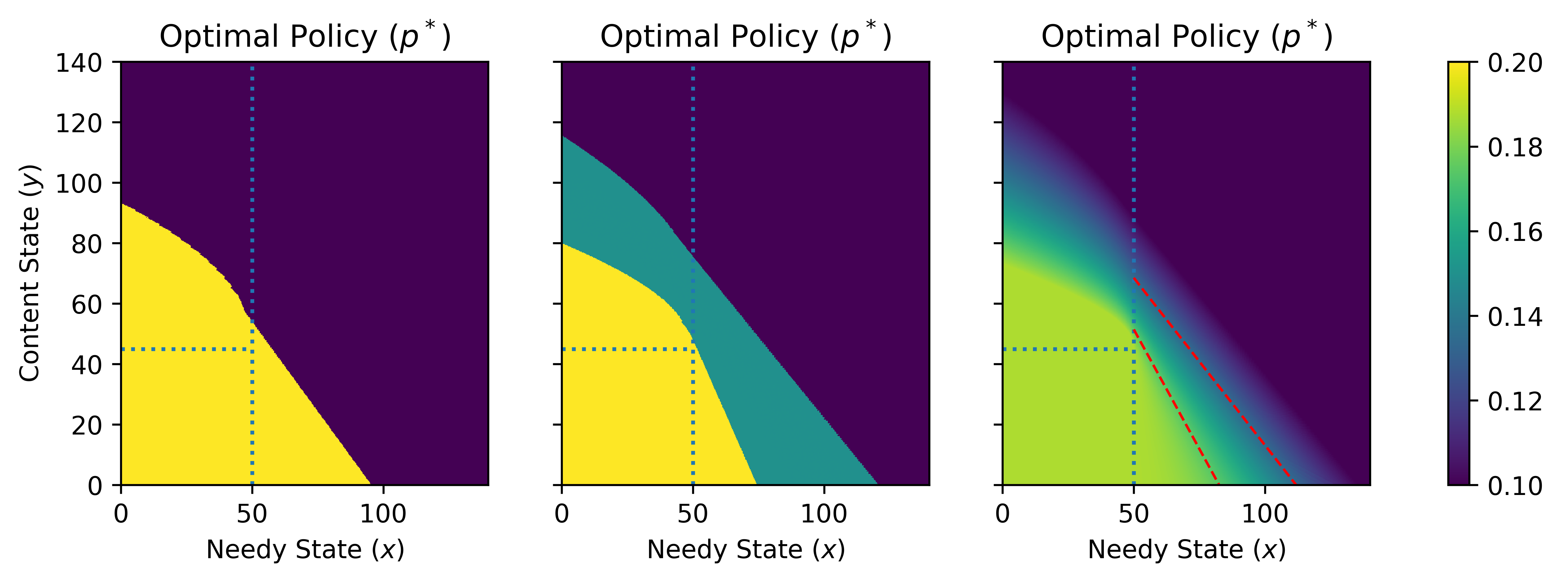
Figure 2: Optimal transient policies under three intervention cost structures: linear $C(p)=5(0.2-p)$ (left), piecewise linear $C(p)=2(0.2-p)+6(0.15-p)^{+}$ (middle), and quadratic $C(p)=50(0.2-p)^{2}$ (right). Other system parameters are $N=50,\lambda=9.5,\mu=1/4,\nu=1/15,p_{l}=0.1,p_{u}=0.2,r=1.0,h=0.25$. Two (isochromatic) contour lines in the ${\mathcal{C}}$ region for the quadratic intervention cost are highlighted in red.

First, we consider a linear intervention cost function $C(p)=5(0.2-p)$. Under this cost structure, no intervention is provided in equilibrium. The optimal transient policy is presented in Figure 2 (left). There is a single boundary separating the $p_{l}$ region and the $p_{u}$ region, and the portion of this boundary lying in ${\mathcal{C}}$ is a line. For states in ${\mathcal{N}}$ the boundary takes the form of a nonlinear curve. Interestingly, at lower Needy states, the policy switches from no intervention to full intervention at lower Content states compared to an extension of the line in ${\mathcal{C}}$. This can be explained noting that the service completion rate is $x(t)\mu$ in this region and hence with a lower number of Content customers the system experiences a slow-down in clearing the customers from the system. As such, the intervention is triggered with a smaller number of Content customers with pending return, in order to compensate for the slow-down.

Next, we consider a piecewise-linear cost $C(p)=2(0.2-p)+6(0.15-p)^{+}$ which has a breakpoint at $C(0.15)=0.1$. Compared to the linear intervention cost which has derivative $C^{\prime}(p)=-0.5$, the partial intervention of $p=0.15$ comes at a lower marginal cost with $C^{\prime}(p)=-0.2$, but moving from partial to full intervention comes at a higher marginal cost with $C^{\prime}(p)=-0.8$. The optimal transient policy is presented in Figure 2 (middle). The policy structure is similar to that of the linear cost. We once again apply no intervention ($p_{l}$) in the bottom-left of the state space, and apply full intervention ($p_{u}$) in the upper-right. However, there is now also a strip in the middle which corresponds to mid-level intervention ($p=0.15$). The boundary between the partial and full intervention regions is less steep than the one between the partial and no-intervention regions.

Finally, we consider a strictly convex intervention cost $C(p)=50(0.2-p)^{2}$. In this case, using Proposition 3.1 we find that the equilibrium optimal policy is to apply a modest level of intervention, yielding a return probability of $p_{\infty}=0.1876$. Figure 2 (right) presents the optimal transient policy. We observe that the policy is monotone with respect to both $x$ and $y$, decreasing from $p_{\infty}$ near the bottom-left to $p_{l}$ in the upper-right. Moreover, this happens continuously such that the policy contours form lines in ${\mathcal{C}}$ as described in Theorem 4.7. Two such lines are highlighted on the figure as examples. We observe from the slopes of these two lines that these contours become less steep as $p^{*}$ decreases, fanning out as we move toward the upper-right. As the system becomes more congested, the Content customers are thus discounted at a smaller rate relative to the Needy customers in determining the level of intervention. This is intuitive since if the queue takes longer to clear, then Content customers contribute more to future congestion costs whereas with a small queue length, the congestion will already have cleared by the time most of the Content customers return.

4.4.2 Implementing the Policy for the Stochastic System.

The fluid policy can be directly translated to an admissible policy for the stochastic system. At each departure epoch $t_{k},k\geq 0$ the return probability is determined through $p^{\tilde{\pi}}(X(t_{k}),Y(t_{k}))$ where $p^{\tilde{\pi}}(\cdot,\cdot)$ is the optimal solution of the transient fluid control problem starting from state $(X(t_{k}),Y(t_{k}))$. Note that the translated policy is re-calculated based on the state of the system at each departure epoch, which may deviate from the predicted fluid trajectory due to stochastic fluctuations.

To illustrate, we present an example for the same system described above under the strictly convex cost function. In Figure 3 we plot the optimal trajectories starting from the initial condition $(80,60)$ overlaid on a sample path of the stochastic queueing system operating under the translated policy and starting from the same initial state. We can see that the fluid trajectories approximately track the sample paths, capturing the first-order dynamics of the stochastic system.

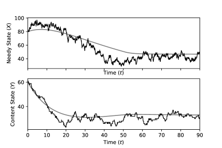
Figure 3: Optimal fluid trajectories starting from the initial state $(80,60)$ overlaid on a sample path of the stochastic system under the translated policy. The intervention cost is $C(p)=50(0.2-p)^{2}$; other cost and system parameters are $N=50,\lambda=9.5,\mu=1/4,\nu=1/15,p_{l}=0.1,p_{u}=0.2,r=1.0,h=0.25$.

5 Time-Varying Arrivals

So far, we have assumed a stationary arrival rate in our analysis. In many service systems, including our motivating healthcare setting, arrival rates are subject to significant temporal variation; see, e.g., Green et al. (2007) and Yom-Tov and Mandelbaum (2014). Hence, in the following, we discuss the application and robustness of the results and policies developed for the stationary system to the case with time-varying arrival rates. Specifically, we assume that the arrival process follows a non-stationary Poisson process with a periodic rate $\lambda(t)$ with period $f$, i.e., $\lambda(t+f)=\lambda(t)$ for all $t\geq 0$, and average (over a period) equal to $\bar{\lambda}$. In addition, we extend the set of admissible policies to allow for time-dependent policies. We continue to rely on fluid approximations to develop insights.

Under time-varying arrivals, the trajectories $(x(t),y(t))$ are governed by

$$\dot{x}(t)=\lambda(t)+\nu y(t)-\mu(x(t)\wedge N),$$ (33)

$$\dot{y}(t)=-\nu y(t)+\mu p(t)(x(t)\wedge N),$$ (34)

for $t\geq 0$. Under a fixed return probability $p<1-\bar{\lambda}/(\mu N)$, we expect the trajectories to converge to a periodic equilibrium (i.e., a cyclic orbit in the state-space) with the same period $f$ as the arrival rate. Paralleling our stationary analysis, if we restrict our attention to policies that converge to a periodic equilibrium, we may interpret $J_{\infty}$ as the optimal long-run average cost. Note that with time-varying arrivals the equilibrium may involve a queue that builds up and empties during the period, and as such $J_{\infty}$ we may also include holding costs. Therefore, the optimal policy may not be constant, and could vary depending on the congestion level.

Consider minimizing the total cost over a long but finite time horizon $T$, plus some time-dependent terminal cost function. While we cannot specify the terminal cost function $\Psi_{T}$, we are still able to gain insights by examining the necessary optimality conditions of a control problem of the form,

$$\min_{p(\cdot)\in{\mathcal{P}}}\int_{0}^{T}h(x(t)-N)^{+}+r\nu y(t)+C(p(t))\mu(x(t)\wedge N)\,dt+\Psi_{T}(x(T),y(T)),$$ (35)

where an admissible policy must satisfy the fluid dynamics in (33)–(34) in addition to (9)–(10). Intuitively, if $T$ is very large, this should approximate the bias-optimal objective with an optimal policy achieving both the optimal long-run average and transient costs.

Applying Pontryagin’s minimum principle to this problem, we observe that as in the stationary case the optimal policy is given by $p^{*}(t)=\argmin_{p}\{C(p)+\gamma_{2}(t)p\}$. We thus pay particular attention to the trajectory of the costate $\gamma_{2}(t)$, since its value determines the optimal policy. The costate trajectories are governed by the same equations (19)-(20), which can be expressed as:

$$\dot{\gamma}_{1}(t) =\begin{cases}-h,&x(t)>N,\\ \mu(\gamma_{1}(t)-C(p^{*}(t))-p^{*}(t)\gamma_{2}(t)),&x(t)\leq N,\end{cases}$$ (36)

$$\dot{\gamma}_{2}(t) =\nu(-\gamma_{1}(t)+\gamma_{2}(t)-r).$$ (37)

The time-varying arrival rate $\lambda(t)$ affects the timing of the transitions when $x(t)$ crosses above and below the capacity $N$. Characterization of an optimal policy hence becomes much more difficult, similar to the case of region ${\mathcal{N}}$ under stationary arrivals. In particular, each entry into or exit from ${\mathcal{C}}$ marks a change in the system of ODEs governing the dynamics, which requires computation of new boundary conditions. As such, we focus on developing an understanding of the parameter regimes where the time-variation has a significant impact on the performance of a policy.

In the case of a fixed probability of return, Yom-Tov and Mandelbaum (2014) report that when the service times are “much longer” than the scale of time variability (e.g., hourly variation in arrival rate and service times in the order of days) the impact of time-variation is small. Similar observations are made in Chan et al. (2014) in a system subject to speedup under a threshold policy. We study the effect of the time-scale of the parameters for our problem by examining the costate trajectories in (36)–(37). The higher the transition rates $\mu$ and $\nu$ (i.e. the shorter the timescales), the faster the costates change. If we fix the period $f$ while increasing the service and time-to-return times (i.e., decrease $\mu$ and $\nu$), we expect to see less variation in $\gamma_{2}$ and hence less variation in the policy. Conversely, holding $\mu$ and $\nu$ unchanged and varying the arrival rate faster would achieve the same. Intuitively, shorter-term fluctuations have less impact on the policy, since they are smoothed out when considering the timescale of the service and return.

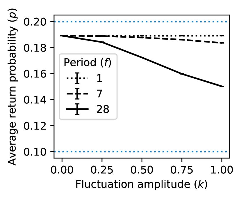
(a) Linear Intervention Cost

(b) Quadratic Intervention Cost

Figure 4: Long-run average probability of return under the fluid policy for three periods and varying amplitudes of the arrival rate. Other system and cost parameters are $N=50,\bar{\lambda}=0.95,\mu=1/4,\nu=1/15$; and $r=1,M=0.5,h=1/4$ with $C(p)=5(0.2-p)$ (left) and $C(p)=50(0.2-p)^{2}$ (right).

We illustrate these effects using simulation experiments. We consider sinusoidal arrival rate functions of the form,

$$\lambda(t)=\bar{\lambda}(1+k\sin(2\pi t/f)),$$ (38)

and vary the fluctuation amplitude $k\in\{0,0.25,0.5,0.75,1.0\}$ as well as the period $f\in\{1,7,28\}$ to capture daily, weekly, and monthly timescales. We fix the other system parameters to $N=50,\bar{\lambda}=0.95,\mu=1/4,\nu=1/15$ and the cost parameters to $r=1,M=0.5,h=1/4$ and consider the same linear and quadratic intervention cost functions from Section 4.4. We compute the fluid policy using the stationary arrival rate $\bar{\lambda}$ and the same implementation described in Section 4.4.2 for the stochastic system but under time-varying arrivals.

Figure 4 presents the long-run average probability of return under the fluid policy for the three periods and varying relative amplitudes. We observe that hourly variations in the arrival rate have effectively no impact. Under strong intra-week fluctuation, we begin to see more frequent interventions, but the impact is still modest. It is only when we move to the extreme case of month-long variation, which has the same order as the service time and time-to-return, that we observe a more sizable impact. We find consistent results with respect to other performance measures, e.g., the long-run average proportion of time all servers are busy; see Appendix 10.

Our experiments suggest that in a parameter regime relevant to our motivating application, namely significant hourly arrival rate variations and service and return times that are in the order of days, our fluid policy that uses the average arrival rate $\bar{\lambda}$ should continue to preform well. We demonstrate the performance of the policy for systems with time-varying arrivals in the numerical study of Section 6.

6 Numerical Experiments

In this section, we first conduct a simulation study to: (1) investigate the performance of the fluid-based control policies for the original stochastic system (with both stationary and time-varying arrivals), and (2) identify parameter regimes where the post-service intervention can lead to significant cost savings. Next, in Section 6.3, we conduct a case study where we examine the robustness and application of the results to the hospital readmission application.

We use a direct translation of the optimal fluid-based policy for the stochastic system described in Section 4.4.2 (referred to as the fluid policy) and evaluate its performance over both finite and infinite-horizon intervals. We evaluate the performance of the fluid policy based on both the long-run expected cost of the system as well as the expected cost over a finite-horizon of 90 days and starting from different initial states. We compare the performance against two benchmark policies:

1. The equilibrium policy which uses the fixed optimal (fluid) long-run average return probability $p_{\infty}$ at all times. This policy ignores the congestion and its associated costs, only considering the direct trade-off between readmission and intervention costs. It can be viewed as an optimistic version of the status-quo practice for the hospital readmission application, where only readmission and intervention costs are considered. By comparing the difference in costs under the fluid policy and the equilibrium policy, we gain an understanding of the value of congestion-awareness.

2. The simple policy which uses the return probability $p_{\infty}$ whenever $X(t_{k})\leq N$, and the lowest possible return probability $p_{l}$ (highest level of intervention) whenever the queue is non-empty. This policy considers congestion, but not the specific level of congestion. By comparing the performance of the fluid policy with that of the simple policy, we thus quantify the value of dynamically adjusting the intervention level in response to varying levels of congestion.

We compare the fluid policy against these benchmarks by estimating the absolute and relative reduction in the expected cost of the system achieved by the policy. The relative reduction is the ratio between the expected cost incurred under the fluid policy and that incurred under the benchmark policy, minus one. We construct a confidence interval for this estimate using Fieller’s method (Fieller 1932).

System parameters. Throughout our experiments, we fix the number of servers at $N=50$ and the service rate at $\mu=1/4$, representing an average service time of 4 days. We vary the return rate in our experiments in $\nu\in\{1/10,1/15,1/20\}$ representing an average time-to-return between 10 and 20 days. We consider the interval of return probabilities $[p_{l},p_{u}]=[0.1,0.2]$. The 20% return probability without intervention is representative of higher-risk patient cohorts for whom one would be interested in intervening. Finally, we vary the exogenous arrival rate $\lambda\in\{9.0,9.5,9.8\}$. Note that in the absence of an intervention (i.e., under a constant return probability $p=0.2$), the arrival rates corresponds to a utilization of 90%-98%.

Cost parameters. We fix the return cost in our experiments at $r=1$, representing a reference value against which the other costs are measured. Note that this cost is charged once for the entire service. Since the average service time is 4 days, the return cost is $0.25$ per day for the average service time. Denote by $M$ the maximum intervention cost corresponding to the lowest return probability. We consider two functional forms for the intervention cost: (1) linear with $C(p)=10M(0.2-p)$ and (2) quadratic with $C(p)=100M(0.2-p)^{2}$. While $C(p_{l})$ and $C(p_{u})$ are identical under both forms, the strict convexity of the quadratic cost offers the ability to partially reduce the readmission probability for a lower marginal cost. As a baseline, we set $M=0.5$, which is half the return cost, but vary $M\in\{0.2,0.5,1.0\}$ in our experiments. Finally, we consider a baseline holding cost rate of $h=0.25$ per day for each customer waiting in queue, equal to the average per-day cost of return. We vary $h\in\{0.05,0.1,0.25,0.5,1.0\}$ in our experiments.

6.1 Stationary Arrivals

We present two sets of experiments. In the first set, we fix the system parameters at their nominal values and vary the cost parameters. In the second set, we fix the cost parameters at their nominal values and vary the arrival and return rates. We present the results under both finite-horizon and infinite-horizon (long-run) settings. For the finite-horizon experiments, we consider three initial state values $(X(0),Y(0))\in\{(25,65),(65,25),(65,65)\}$ and examine the performance of the policies over a 90-day horizon.

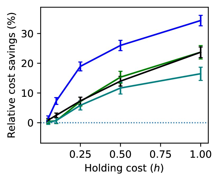
(a) $M=0.2$

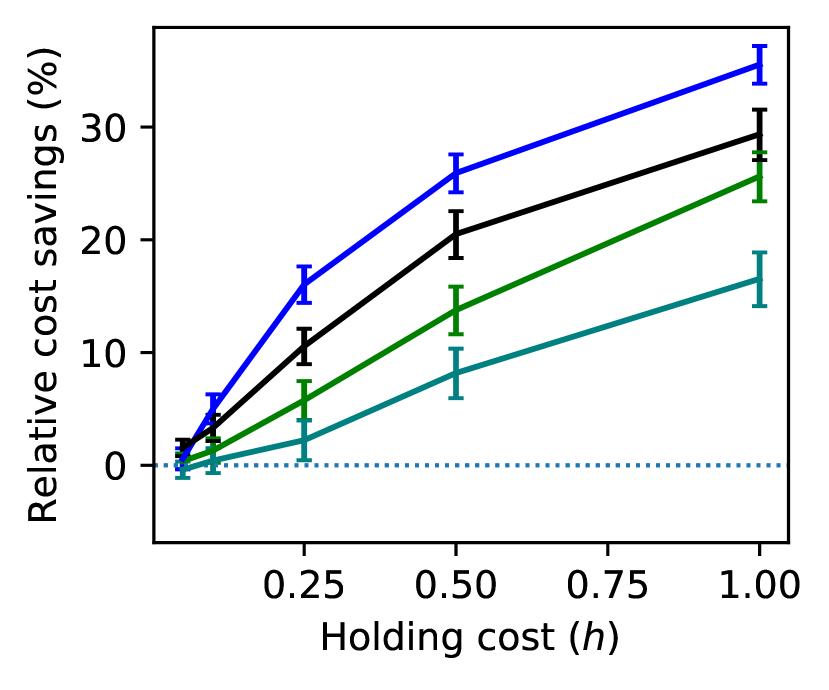
(b) $M=0.5$

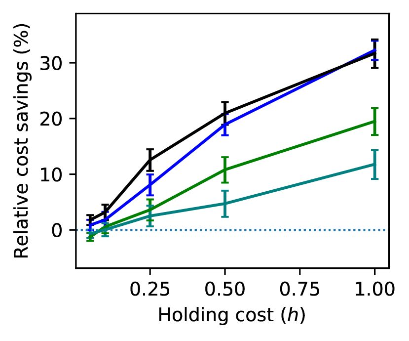
(c) $M=1.0$

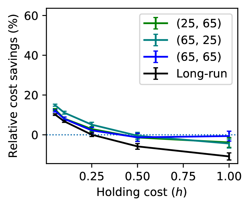
(d) $M=0.2$

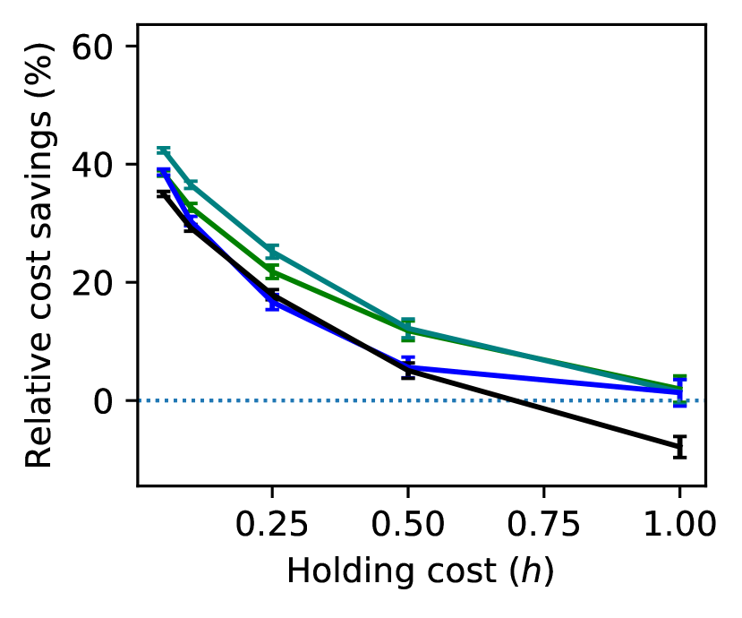
(e) $M=0.5$

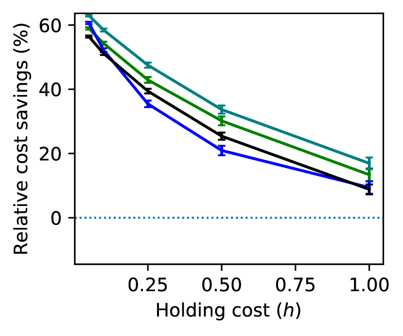
(f) $M=1.0$

Figure 5: Relative reduction in expected cost for both finite-horizon and long-run experiments under the fluid policy with respect to the equilibrium policy (top row) and simple policy (bottom row) under the quadratic intervention cost and for different values of cost parameters. System parameters are fixed at $N=50,\lambda=0.95,\mu=1/4,\nu=1/15$ and and the return cost is normalized at $r=1$.

We begin by examining the performance of the fluid policy for different cost parameters. Figure 5 presents the relative reduction in expected cost under the fluid policy compared to the equilibrium (top row) and simple (bottom row) policies for the quadratic intervention cost function and under varying maximum intervention cost $M$ and holding cost $h$. We observe that when the intervention is relatively expensive, i.e., comparable to the return cost, and the holding cost is moderate, i.e., $h=0.5$, the fluid policy outperforms the benchmarks with respect to both the long-run average and finite-horizon costs. The cost savings are quite significant, e.g., for $h=0.5$ and $M=1$ we observe a 21.0% reduction in the expected long-run average cost compared to the equilibrium (no intervention) policy and a 25.4% reduction compared to the simple policy. If the intervention is cheap and the holding cost is large, the simple policy can outperform the fluid policy. Similarly if the holding cost is very small and the intervention is expensive, the equilibrium policy could lead to the same or slightly lower cost. Nevertheless, the fluid policy never performs worse than both benchmarks. In addition, we observe that the absolute differences are very small in these cases. In contrast, when the fluid policy outperforms the benchmarks, both absolute and relative savings are significant; see Appendix 10 for details.

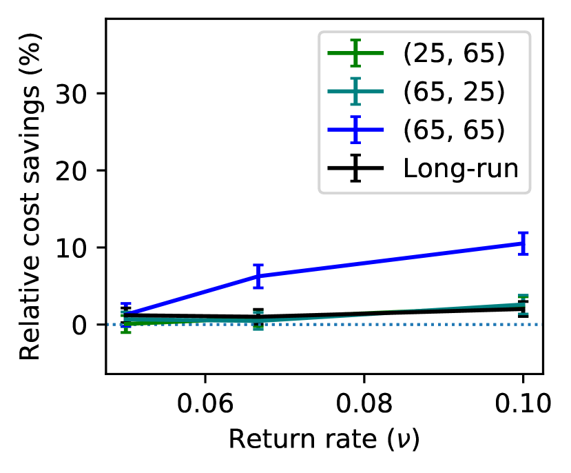
(a) $\lambda=9.0$

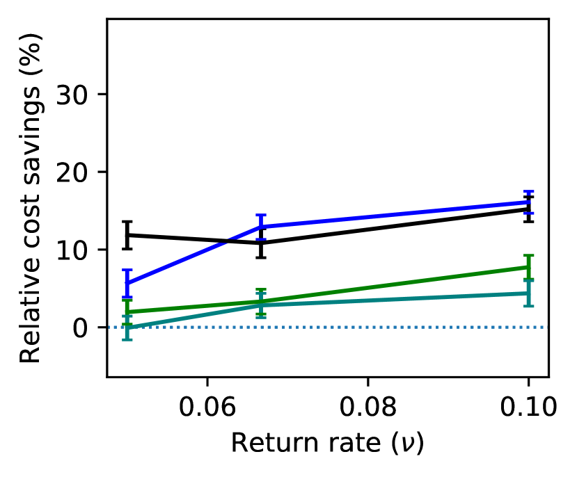
(b) $\lambda=9.5$

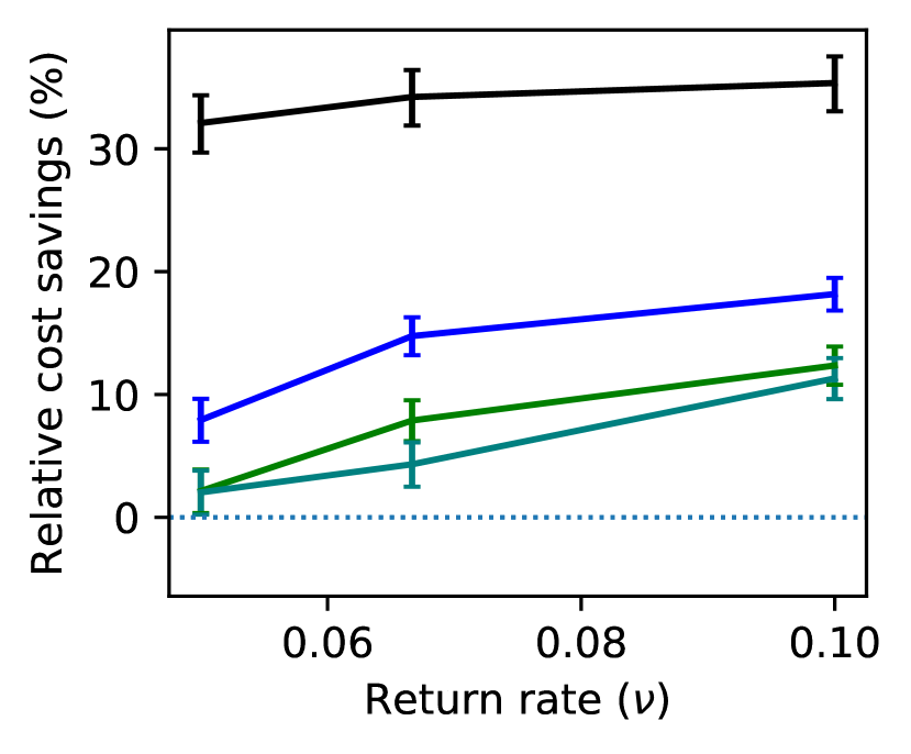
(c) $\lambda=9.8$

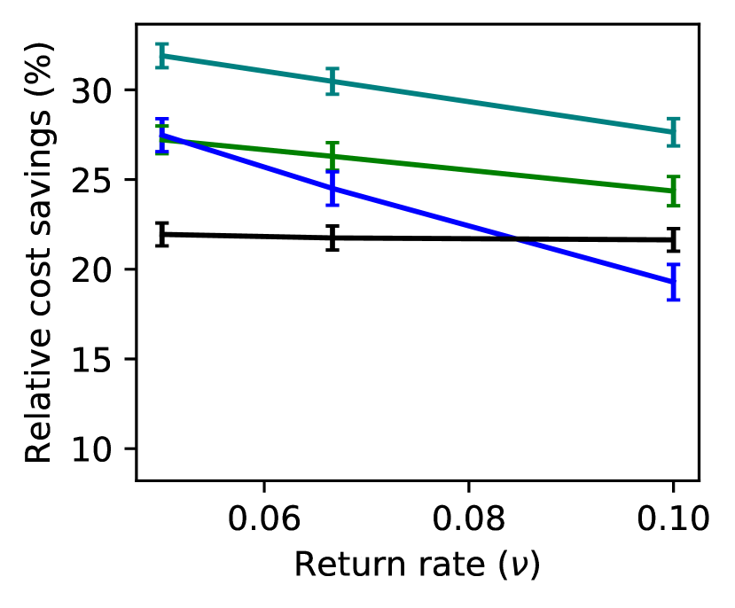
(d) $\lambda=9.0$

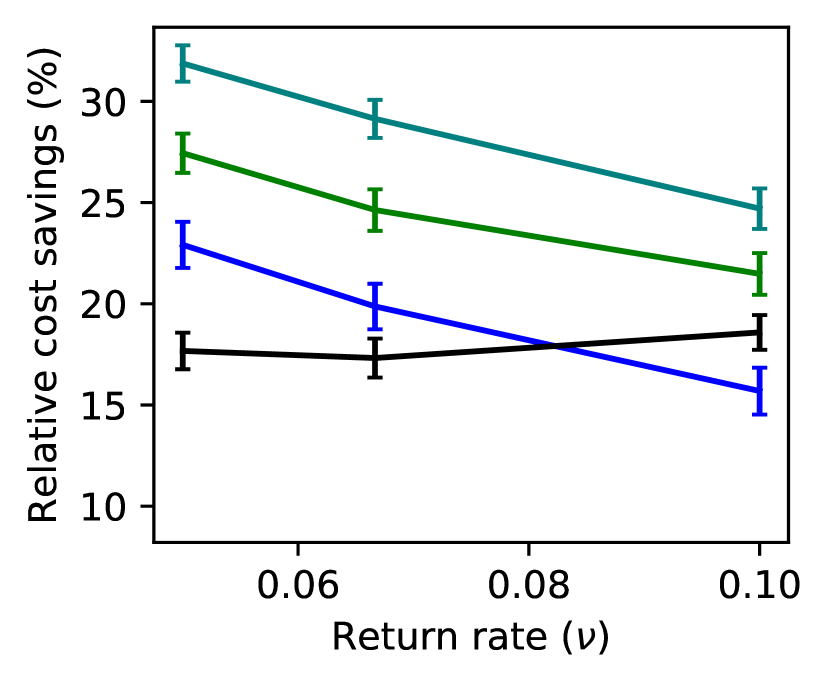
(e) $\lambda=9.5$

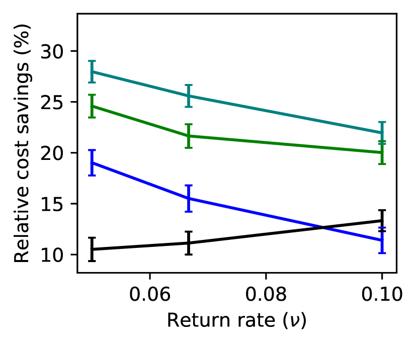
(f) $\lambda=9.8$

Figure 6: Relative reduction in expected cost for both finite-horizon and long-run experiments under the fluid policy with respect to the equilibrium policy (top row) and simple policy (bottom row) under the quadratic intervention cost and for different values of arrival $\lambda$ and return $\nu$ rates. Other cost and system parameters are fixed at $N=50,\mu=1/4,r=1,M=0.5,h=1/4,C(p)=50(0.2-p)^{2}$.

Next, we examine the performance of the fluid policy for different system loads and return rates. Figure 6 presents the relative reduction in expected cost under the fluid policy compared to the equilibrium (top row) and simple (bottom row) policies for the quadratic intervention cost function and under varying arrival rates $\lambda$ and return rates $\nu$, while fixing the cost parameters at their nominal values, i.e., $h=1/4,M=0.5$ and $r=1$. We first discuss the impact of return rate. We observe that the return rate can have a significant effect on the transient cost savings, whereas the long-run average savings are less sensitive. As the return rate increases, the value of adjusting the intervention in response to congestion increases and hence the cost savings compared to the equilibrium policy increase. At the same time, the cost savings compared to the simple policy decrease but remain positive. Next, we consider the impact of the arrival rate. As the arrival rate increases, the system load and hence the congestion increases, making it more valuable to increase the intensity of the intervention in response to congestion. Therefore, we observe a significant increase in cost savings compared to the equilibrium policy both for the long-run and transient experiments. As expected, when compared to the simple policy, the cost savings decrease with higher arrival rates but remain positive.

We conduct the same experiments under the linear intervention cost function. Overall, the observations remain similar but the cost savings compared to the equilibrium (no intervention) policy can be higher when positive. The detailed results can be found in Appendix 10.

The above numerical results lead to two key observations: First, we observe significant cost savings compared to the equilibrium policy which is agnostic to congestion, demonstrating that accounting for the congestion cost can make it optimal to intervene in cases where otherwise it may not seem economical to do so. Under none of the simulated parameter regimes did the congestion-agnostic equilibrium policy $p_{\infty}$ equal the lowest value $p_{u}$. The additional intervention applied by the fluid policy became economical only due to the consideration of holding costs, especially when the starting state was far from the equilibrium. Moreover, when the holding cost was moderate or high, these savings were seen even in the long-run. From time to time, stochastic fluctuations bring the system away from the equilibrium point and into ${\mathcal{C}}$, so the fluid policy’s ability to efficiently steer the system back toward the equilibrium remains valuable.

Second, we find that in a relevant parameter regime to our hospital readmission application, namely costly interventions and moderate holding costs (relative to cost of return), dynamically adjusting the intervention level based on the observed congestion can lead to significant cost savings.

6.2 Time-Varying Arrivals

In this section, we examine the robustness of the observations made in the previous section for systems with time-varying arrivals. We use the same sinusoidal arrival rate as in (38) in our simulation experiments and evaluate the performance of the fluid policy (which uses the average arrival rate $\bar{\lambda}$) against the two benchmarks for varying periods and amplitudes of the arrival rate.

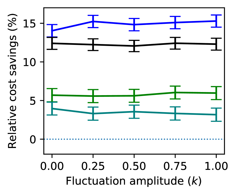
(a) $f=1$

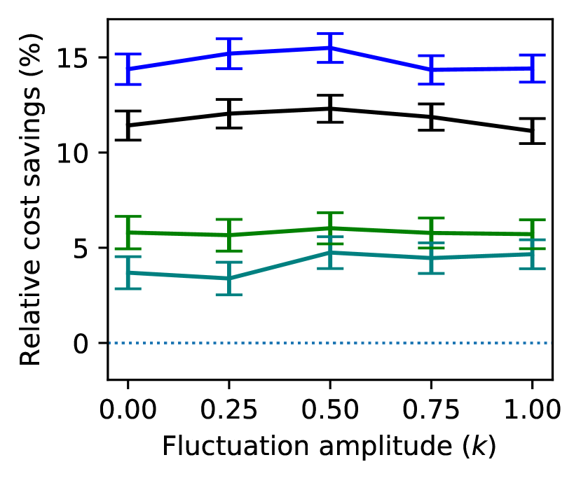
(b) $f=7$

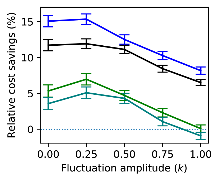
(c) $f=28$

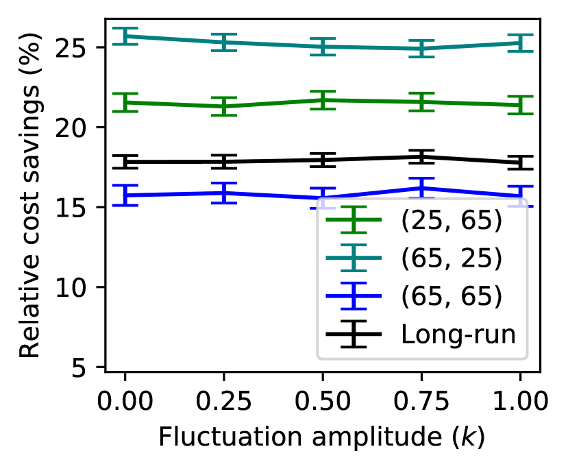
(d) $f=1$

(e) $f=7$

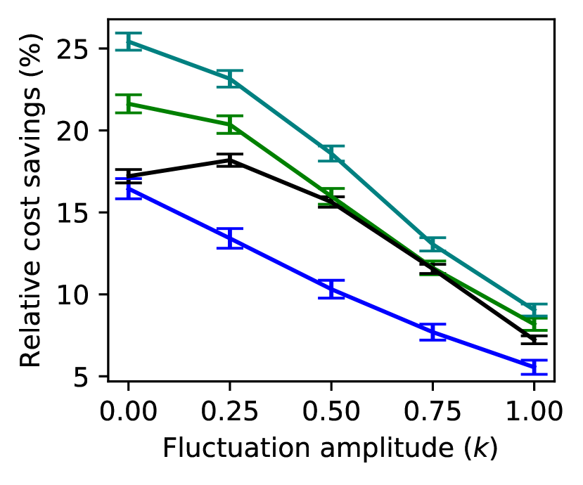
(f) $f=28$

Figure 7: Relative reduction in expected cost under the fluid policy with respect to the equilibrium policy (top row) and simple policy (bottom row) under different time-varying arrival rate functions. System and cost parameters are fixed at $N=50,\bar{\lambda}=0.95,\mu=1/4,\nu=1/15,r=1,h=1/4,C(p)=50(0.2-p)^{2}$.

We observe that as long as the scale of service and time-to-return times are large relative to the scale of time-variation, the fluid policy (which ignores time-variation) still performs well even when the amplitude of the variation is high. We illustrate this by considering the quadratic cost function and baseline system parameters where the average service time and time-to-return are $1/\mu=4$ and $1/\nu=15$ days, respectively. Figure 7 presents the relative reduction in expected cost achieved under the fluid policy in contrast to the two benchmark policies and for different time-variation scales and amplitudes. In the cases of intra-day and intra-week variation, the cost savings remain fairly consistent even as we increase the amplitude of the fluctuation. In these cases, the fluid policy consistently outperforms the two benchmark policies. It is only when the period is lengthened to 28 where we observe a reduction in the cost savings for larger amplitude values. We observe consistent results for other system parameters and cost functions; see Appendix 10 for the same experiments under the linear cost function.

6.3 Case Study: Hospital Readmission

In this section, we conduct a numerical study using parameters that are calibrated based on a real hospital setting and post-discharge readmission intervention plan reported in the literature. In doing so, we further relax some of our modeling assumptions to examine the robustness of our observations.

Cost and intervention parameters. Our intervention and cost parameters are modeled after a transitional care program for heart failure patients studied in Stauffer et al. (2011). The intervention involves multiple home visits after discharge by an Advanced Practice Nurse (APN) who is also available for telephone calls. The cost of intervention per patient is $M=1110$ and the cost of a readmission is $r=5000$. Estimated readmission probabilities with and without the intervention are $p_{l}=0.081$ and $p_{u}=0.141$, respectively, i.e., the intervention has a 42% efficacy. Since the intervention does not have multiple levels, we construct the intervention cost function $C(\cdot)$ by interpolating the cost of the two extremes on the interval $[p_{l},p_{u}]$. However, we know by Proposition 4.4 that the resulting fluid policy will be bang-bang, always choosing either $p_{u}$ (no intervention) or $p_{l}$ (intervention). We vary the holding cost $h\in\{500,1000,1500,2000,2500,3000\}$ in our experiments.

From Corollary 3.3, we know that the equilibrium policy under a linear intervention cost is determined by comparing the expected total cost savings associated with intervention against the intervention cost. Under the costs above, the expected lifetime savings of $r(p_{u}-p_{l})/(1-p_{u})=349.2$ are $0.31$ times the intervention cost $M=1110$. This is somewhat higher than the corresponding value of $0.25$ under the baseline parameters of the numerical experiments in Section 6.1. We therefore have a higher incentive to intervene, and expect the fluid policy to be closer to the simple policy.

System parameters. We calibrate the parameters of our model based on those of the Internal Ward A of Ramban Hospital (referred to as Ward A hereafter) described in Armony et al. (2015). We set the number of servers to the number of beds of Ward A, i.e., $N=45$ and use the Log-Normal distribution fitted to Length-of-Stay (LOS) data, which has log-mean $1.38$, log-standard deviation $0.83$, and mean $1/\mu=5.6$. The arrival rate follows a non-stationary Poisson process with rate,

$$\lambda(t)=\begin{cases}6.14(1-0.8\sin(2\pi t)),&t\ (\mathrm{mod}\ 7)\leq 5,\\ 5.32(1-0.8\sin(2\pi t)),&t\ (\mathrm{mod}\ 7)>5.\end{cases}$$ (39)

The overall average arrival rate of $\bar{\lambda}=5.91$ is based on Ward A, which receives $206.3$ patients per month. We adjust this value by a factor of $1-p_{u}$, removing readmissions to obtain the net arrival rate of new patients for our case study. In addition, we add hourly fluctuations with relative amplitude of $0.8$, and reduce weekend arrival rates compared to weekdays. The return times follow a distribution with density $0.057\exp(-x/25),x\in(0,30)$ with mean $\nu=1/12.07$, equivalent to an exponential distribution with mean $25$, conditional on being less than 30. These parameters yield an average load of $\bar{\lambda}/\mu(1-p_{h})=38.6$ in the absence of intervention, corresponding to a $\rho=0.86$ utilization.

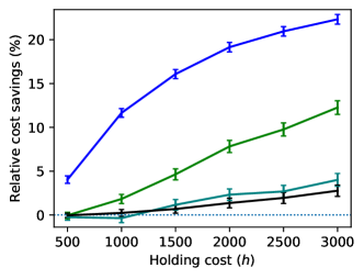
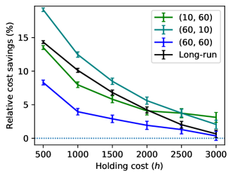
Figure 8: Relative reduction in expected cost in the case study as measured against the equilibrium policy (left) and the simple policy (right) for different holding cost values.

Results. Figure 8 presents the relative reduction in expected cost savings under the fluid policy compared to the two benchmarks. As in Section 6 we consider both the long-run average cost, and transient cost over a 90-day horizon starting with three different initial states. Despite the relaxations to the model assumptions and lower utilization, the fluid policy performs the same or better than both benchmark policies. In addition, our qualitative observations in Section 6.1 continue to hold.

As reported in Stauffer et al. (2011) the intervention is not economical when only considering the costs of readmission versus intervention. However, even for relatively small holding costs, the intervention could be economical for a system starting from a state far from the equilibrium. For larger holding cost values, we observe considerable savings through the intervention specially over a finite horizon. The savings are also considerably larger compared to the simple policy, as long as the holding cost is not too high.

Finally, we examine the tradeoff between direct costs of returns and intervention, versus the average queue-length under the fluid policy. In doing so, we treat the holding cost as a parameter and vary it in the same range as before to obtain different pairs of average queue-length and costs. In addition to the case with 86% utilization, we also present the results for 90% utilization. Figure 9 presents the tradeoff curves for the long-run average and two finite-horizon cases. Note that each point on the curves corresponds to a certain holding cost. Increasing the holding cost leads to higher intervention costs, but lower return costs and queue-length. The tradeoff curves appear to be convex, that is the average queue-length can be reduced in return for a small increase in direct costs. We note that the smaller values of queue-length in the long-run average are due to the time-varying arrival rate, and the peak congestion over each period (and the corresponding reduction) is larger.

(a) $(X^{0},Y^{0})=(10,60),\rho=0.85$

(b) $(X^{0},Y^{0})=(60,10),\rho=0.85$

(c) Long-run, $\rho=0.85$

(d) $(X^{0},Y^{0})=(10,60),\rho=0.90$

(e) $(X^{0},Y^{0})=(60,10),\rho=0.90$

(f) Long-run, $\rho=0.90$

Figure 9: Tradeoff between direct (readmission and intervention) costs and queue-length for long-run average and finite-horizon costs with different initial conditions. The star and triangle symbols respectively correspond to the equilibrium and simple policy.

7 Conclusion and Discussion

In this work, we propose and study a new control problem for queueing systems with returns. Our model captures the tradeoff between the cost of post-service interventions and the benefits through reduced readmissions including reduced congestion costs. We study associated fluid control problems and characterize the structure of the long-run average and transient optimal policies under a general convex intervention cost. Through our analysis of the fluid control problems, we obtain approximately optimal policies for the stochastic system and gain insights into the structure of congestion-aware intervention policies. In particular, under a piecewise linear cost function, the policy divides the state-space into as many regions as there are pieces in the cost function, and prescribes a different level of intervention intensity (probability of return) in each region. This intuitive structure motivates the design of practical surge protocols that economically use post-discharge interventions to recover from highly congested states.

Our structural results provide insights into the impact of both Content and Needy states on the intensity of the intervention. In practice, the Content state is often not directly observable. However, the value of the Content state can be estimated through predictive models and then used to compute the intervention level. When the intervention cost is piecewise, the intervention level remains relatively insensitive to the precise value of the Content state. As such, small prediction errors are likely to not impact the level of intervention. In this work, we have utilized a parsimonious model to understand the interaction between congestion and post-service interventions. An interesting area for future work would be the integration of our policies with personalized predictions of readmission risk to develop practical policies and test their performance using high-fidelity simulation models.

Our characterization of the transient optimal policy relies on the notion of bias-optimality for fluid control problems. The proposed cost criteria can be utilized to study transient policies for other multiserver queueing control problems where the total cost of the system does not remain finite over an infinite horizon. Compared to using state-dependent constraints, this approach allows for an easier application of Pontryagin’s Minimum Principle. We believe this approach is applicable to other complex queueing control problems.

Proofs and Supplementary Numerical Experiments

8 Proofs of Lemmas and Propositions

Proof 8.1

Proof of Proposition 3.1. $(i)$ To prove the first claim, we bound the time at which the fluid state reaches region ${\mathcal{A}}$ starting from a given initial state. Consider $\hat{y}$ whose dynamics are governed by:

$$\dot{\hat{y}}(t)=\mu Np_{u}-\nu\hat{y}(t),$$ (40)

for $t\geq 0$ and starting from $\hat{y}(0)=y^{0}$. Since $\dot{y}(t)-\dot{\hat{y}}(t)\leq-\nu(y(t)-\hat{y}(t))$ and $y(0)-\hat{y}(0)=0$, Gronwall’s inequality yields $y(t)-\hat{y}(t)\leq 0$ for all $t\geq 0$. Therefore, $\hat{y}$ is an upper bound for $y$.

Next, note that since $\lim_{t\to\infty}\hat{y}(t)=(\mu Np_{u})/\nu<(\mu N-\lambda)/\nu$, there exists a time $t_{1}<\infty$, such that $y(t)\leq\hat{y}(t)\leq(\mu N-\lambda)/\nu$ for all $t\geq t_{1}$ and under all policies $p(\cdot)\in{\mathcal{P}}$.

Define $t_{\mathcal{A}}:=t_{1}+\frac{x_{0}+y_{0}+\lambda t_{1}}{\mu N(1-p_{u})-\lambda}+1$. Under a given policy $p\in{\mathcal{P}}$, if $x(t_{1})\leq N$, then $(x(t_{1}),y(t_{1}))\in{\mathcal{A}}$. If $x(t_{1})>N$, note that $x(t_{1})+y(t_{1})\leq x^{0}+y^{0}+\lambda t_{1}$, since the total number of customers (both Needy and Content) always grows at a rate of at most $\lambda$. As long as $x(t)>N$, all servers are busy and the total number of customers in the system decreases at a rate of at least $\mu N(1-p_{u})-\lambda$ (which is positive by Assumption 2.1). The queue therefore must empty at some time before $t_{\mathcal{A}}$, else there would be a negative number of customers remaining in the system, an impossibility.

Therefore under any policy $p(\cdot)\in{\mathcal{P}}$, there is a $t\leq t_{\mathcal{A}}$ such that $(x(t),y(t))\in{\mathcal{A}}$. Applying the result of part (ii) then gives us $(x(t_{\mathcal{A}}),y(t_{\mathcal{A}}))\in{\mathcal{A}}$.

$(ii)$ Since the trajectory $(x(t),y(t))$ is (almost everywhere) differentiable, it suffices to show that its gradient points inward along the boundaries of ${\mathcal{A}}$ under any admissible policy. Along the vertical boundary line $x=N$, the gradient points leftward:

$$\dot{x}(t) =\lambda+\nu y(t)-\mu(x(t)\wedge N)$$ (41)

$$=\lambda+\nu y(t)-\mu N$$ (42)

$$\leq\lambda+(\mu N-\lambda)-\mu N=0,$$ (43)

where the inequality in (43) is strict for $y(t)<(\mu N-\lambda)/\nu$. Along the horizontal boundary line $y=(\mu N-\lambda)/\nu$, the gradient points downward:

$$\dot{y}(t) =-\nu y(t)+\mu p(t)(x(t)\wedge N)$$ (44)

$$=-(\mu N-\lambda)+\mu p(t)(x(t)\wedge N)$$ (45)

$$\leq\lambda-\mu N+\mu p_{u}N$$ (46)

$$=\lambda-\mu N(1-p_{u})<0.$$ (47)

Finally, at the top-right corner $(N,(\mu N-\lambda)/\nu)$ the gradient points straight downwards with $\dot{x}(t)=0$ and $\dot{y}(t)<0$. Note that since $\dot{y}<0$ and $\dot{x}=0$, we can see that $\dot{x}=\lambda-\nu y-\mu(x\wedge N)$ is decreasing. The trajectory will thus curve inwards and the state will remain in ${\mathcal{A}}$.

Proof 8.2

Proof of Proposition 3.2. Differentiating $J(p)$ we have,

$$J^{\prime}(p)=\frac{(1-p)C^{\prime}(p)+C(p)+r}{1-p}.$$ (48)

Denote the numerator of (48) by $q(p):=(1-p)C^{\prime}(p)+C(p)+r$. The denominator of (48) is positive on $[p_{l},p_{u}]$, so the sign of $q(p)$ determines the sign of $J^{\prime}(p)$. Since $C(p)$ is convex by Assumption 2, the derivative $q^{\prime}(p)=(1-p)C^{\prime\prime}(p)$ is non-negative. It follows that the sign of $J^{\prime}(p)$ is non-decreasing. Therefore $J(p)$ is either U-shaped or monotone, and its critical points (if any) form a closed interval.

Since $q(p)$ is non-decreasing, it is minimized at $p_{l}$ and maximized at $p_{u}$. If $q(p_{l})\geq 0$, then $J^{\prime}(p)$ is non-negative on ${\mathcal{P}}$ and thus $J(p)$ is minimized at $p_{l}$. Similarly, if $q(p_{u})\leq 0$, then $J^{\prime}(p)$ is non-positive on $[p_{l},p_{u}]$ and $J(p)$ is minimized at $p_{u}$. Otherwise, $q(p_{l})<0<q(p_{u})$, implying the existence of a root of $q(p)$, i.e., a critical point of $J(p)$ in the interior of $[p_{l},p_{u}]$.

Proof 8.3

Proof of Proposition 4.1. Since $(x^{0},y^{0})\in{\mathcal{A}}$, by Proposition 3.1 the queue will remain empty for all $t\geq 0$. We verify the correctness of the value function using the Hamilton-Jacobi-Bellman (HJB) equations. Here wef suppress the reference to the specific horizon length $T$ since the proof does not depend on its specific value.

$$\dot{V}(x,y,t)+\min_{p}\left\{\dot{x}(t)V_{x}(x,y,t)+\dot{y}(t)V_{y}(x,y,t)+r\nu y+C(p)\mu x-J_{\infty}\right\}$$ (49)

$$\quad=0+\min_{p\in{\mathcal{P}}}\left\{(\lambda+\nu y-\mu x)\frac{rp_{\infty}+C(p_{\infty})}{1-p_{\infty}}+(-\nu y+\mu xp)\frac{r+C(p_{\infty})}{1-p_{\infty}}+r\nu y+C(p)\mu x-J_{\infty}\right\}$$ (50)

$$\quad=\mu x\left(-\frac{rp_{\infty}+C(p_{\infty})}{1-p_{\infty}}+\min_{p\in{\mathcal{P}}}\left\{\frac{r+C(p_{\infty})}{1-p_{\infty}}p+C(p)\right\}\right)$$ (51)

$$\quad=\mu x\left(-\frac{rp_{\infty}+C(p_{\infty})}{1-p_{\infty}}+\frac{r+C(p_{\infty})}{1-p_{\infty}}p_{\infty}+C(p_{\infty})\right)$$ (52)

$$\quad=0.$$ (53)

It is easy to verify that the quantity minimized in (51) is convex with critical point $p_{\infty}$, and hence minimized at $p_{\infty}$. Additionally, we have $V(x,y,T)=\Psi(x,y)$ by definition. The HJB equations are thus satisfied. It follows that $V(x,y,t)$ is the value function for $(x,y)\in{\mathcal{A}}$, and the optimal policy is given by $p(t)=p_{\infty}$ for all $t\geq 0$.

Proof 8.4

Proof of Proposition 4.2. We prove the proposition by obtaining finite lower and upper bounds for the value function. By Proposition 3.1, there is a bound $t_{\mathcal{A}}$ such that $t_{\mathcal{A}}\in{\mathcal{A}}$ under any policy $p(t)$, and that $(x(t),y(t))\in{\mathcal{A}}$ for all $t\geq t_{\mathcal{A}}$ as well.

We will bound the integral up to a large finite time $T\geq t_{\mathcal{A}}$. We can split the objective into an integral up to time $t_{\mathcal{A}}$ and another integral from $t_{\mathcal{A}}$ onwards, and obtain a lower bound by ignoring the costs incurred before $t_{\mathcal{A}}$.

$$\min_{p(\cdot)}\int_{0}^{T}h(x(t)-N)^{+}+r\nu y(t)+C(p(t))\mu(x(t)\wedge N)-J_{\infty}\,dt$$ (54)

$$=\min_{p(\cdot)}\bigg{\{}\int_{t_{\mathcal{A}}}^{T}h(x(t)-N)^{+}+r\nu y(t)+C(p(t))\mu(x(t)\wedge N)-J_{\infty}\,dt$$ (55)

$$\qquad+\int_{0}^{t_{\mathcal{A}}}h(x(t)-N)^{+}+r\nu y(t)+C(p(t))\mu(x(t)\wedge N)-J_{\infty}\,dt\bigg{\}}$$ (56)

$$\geq\min_{p(\cdot)}\left\{\int_{t_{\mathcal{A}}}^{T}h(x(t)-N)^{+}+r\nu y(t)+C(p(t))\mu(x(t)\wedge N)-J_{\infty}\,dt\right\}-J_{\infty}t_{\mathcal{A}}$$ (57)

In addition, because $T\geq t_{\mathcal{A}}$, we are guaranteed that $(x(T),y(T))\in{\mathcal{A}}$ and therefore that $\Psi(x(T),y(T))\leq\Psi(N,(\mu N-\lambda)/\nu)$. Adding a term $\Psi(x(T),y(T))$ to the objective yields the value function from Proposition 4.1, and thus increases the minimum by at most $\Psi(N,(\mu N-\lambda)/\nu)$. This yields the inequalities below.

$$\min_{p(\cdot)}\left\{\int_{t_{\mathcal{A}}}^{T}h(x(t)-N)^{+}+r\nu y(t)+C(p(t))\mu(x(t)\wedge N)-J_{\infty}\,dt\right\}-J_{\infty}t_{\mathcal{A}}$$ (58)

$$\geq\min_{p(\cdot)}\left\{\int_{t_{\mathcal{A}}}^{T}h(x(t)-N)^{+}+r\nu y(t)+C(p(t))\mu(x(t)\wedge N)-J_{\infty}\,dt+\Psi(x(T),y(T))\right\}$$ (59)

$$\qquad-\Psi\left(N,\frac{\mu N-\lambda}{\nu}\right)-J_{\infty}t_{\mathcal{A}}$$ (60)

$$=\Psi(x(t_{\mathcal{A}}),y(t_{\mathcal{A}}))-\Psi\left(N,\frac{\mu N-\lambda}{\nu}\right)-J_{\infty}t_{\mathcal{A}}>-\infty.$$ (61)

We thus have a finite lower bound independent of $T$. Taking $T\to\infty$ makes this a lower bound on the infinite-horizon problem.

We obtain an upper bound in a similar fashion. Since the total number of customers (both Needy and Content) grows at a rate of at most $\lambda$, we know that $K:=x^{0}+y^{0}+\lambda t_{\mathcal{A}}<\infty$ is an upper bound on $x(t)+y(t)$ (as well as $x(t)$ and $y(t)$ individually) for all $t\leq t_{\mathcal{A}}$. We can thus place a finite bound on the costs up to time $t_{\mathcal{A}}$:

$$\int_{0}^{t_{\mathcal{A}}}h(x(t)-N)^{+}+r\nu y(t)+C(p(t))\mu(x(t)\wedge N)-J_{\infty}\,dt\leq(hK+r\nu K+C(p_{l})N-J_{\infty})t_{\mathcal{A}}.$$ (62)

Since $\Psi(x(T),y(T))\geq 0$, adding the terminal cost to the objective yields an upper bound. We thus have the following inequality:

$$\min_{p(\cdot)}\int_{0}^{T}h(x(t)-N)^{+}+r\nu y(t)+C(p(t))\mu(x(t)\wedge N)-J_{\infty}\,dt$$ (63)

$$\leq\min_{p(\cdot)}\left\{\int_{t_{\mathcal{A}}}^{T}h(x(t)-N)^{+}+r\nu y(t)+C(p(t))\mu(x(t)\wedge N)-J_{\infty}\,dt\right\}$$ (64)

$$\qquad+(hK+r\nu K+C(p_{l})N-J_{\infty})t_{\mathcal{A}}$$ (65)

$$\leq\min_{p(\cdot)}\left\{\int_{t_{\mathcal{A}}}^{T}h(x(t)-N)^{+}+r\nu y(t)+C(p(t))\mu(x(t)\wedge N)-J_{\infty}\,dt+\Psi(x(T),y(T))\right\}$$ (66)

$$\qquad+(hK+r\nu K+C(p_{l})N-J_{\infty})t_{\mathcal{A}}$$ (67)

$$=\Psi(x(t_{\mathcal{A}}),y(t_{\mathcal{A}}))+(hK+r\nu K+C(p_{l})N-J_{\infty})t_{\mathcal{A}}<\infty.$$ (68)

We therefore have a finite upper bound independent of $T$, and taking $T\to\infty$ makes this an upper bound on the infinite-horizon problem.

Proof 8.5

Proof of Proposition 4.3. It is clear that $J_{\infty}$ is an upper bound for the minimum long-run average cost, since it is attained by the equilibrium policy. Conversely, suppose for a contradiction that there exists a better policy $p(t)$ with long-run average cost of $J_{\infty}-\varepsilon$ for some $\varepsilon>0$:

$$\limsup_{T\to\infty}\frac{1}{T}\int_{0}^{T}h(x-N)^{+}+r\nu y+\mu C(p(t))(x\wedge N)\,dt=J_{\infty}-\varepsilon.$$ (69)

By definition, there exists a $T_{0}>0$ such that for all $T\geq T_{0}$:

$$\frac{1}{T}\int_{0}^{T}h(x(t)-N)^{+}+r\nu y(t)+\mu C(p(t))(x(t)\wedge N)\,dt<J_{\infty}-\frac{\varepsilon}{2},$$ (70)

implying that,

$$\int_{0}^{T}h(x(t)-N)^{+}+r\nu y(t)+\mu C(p(t))(x(t)\wedge N)-J_{\infty}\,dt<-\frac{\varepsilon T}{2}.$$ (71)

Taking $T\to\infty$ then yields divergence to $-\infty$.

Proof 8.6

Proof of Proposition 4.4. The claim follows from a simple application of the minimum principle. Under a linear intervention cost $C(p)=M\frac{p_{u}-p}{p_{u}-p_{l}}$, we have:

$$\frac{\partial}{\partial p}H(x(t),y(t),p,t) =\mu(x(t)\wedge N)(C^{\prime}(p)+\gamma_{2}(t)p)$$ (72)

$$=\mu(x(t)\wedge N)\left(-\frac{M}{p_{u}-p_{l}}+\gamma_{2}(t)\right).$$ (73)

Thus the Hamiltonian is increasing with respect to $p$ if $\gamma_{2}(t)>\frac{M}{p_{u}-p_{l}}$ and decreasing otherwise. Since $p^{*}(t)$ must minimize the Hamiltonian, it follows that we take $p^{*}(t)=p_{u}$ when $\gamma_{2}(t)>\frac{M}{p_{u}-p_{l}}$ and $p^{*}(t)=p_{u}$ otherwise. If $\gamma_{2}(t)=\frac{M}{p_{u}-p_{l}}$, then we are indifferent to all values of $[p_{l},p_{u}]$, however, this can be shown to only occur momentarily and is hence inconsequential.

Proof 8.7

Proof of Proposition 4.6.

The policy $p^{*}(t)$ is chosen to minimize the Hamiltonian function:

$$h(x-N)^{+}+r\nu y+C(p)\mu(x\wedge N)-J_{\infty}+(\lambda+\nu y-\mu(x\wedge N))\gamma_{1}(t)+(-\nu y+\mu p(x\wedge N))\gamma_{2}(t).$$ (74)

Eliding the terms that do not depend on $p$, we are left with:

$$\mu(x\wedge N)(C(p)+\gamma_{2}(t)).$$ (75)

It thus suffices to minimize the expression $\phi_{t}(p)=C(p)+\gamma_{2}(t)p$, which exactly represents the cost trade-off for a Needy patient finishing service at time $t$. We incur an immediate intervention cost of $C(p)$, and the patient has a probability $p$ of moving to the Content state (or, in the fluid context, the amount of fluid in the Content state increases by $p$ for every unit of fluid finishing service). Since the costate $\gamma_{2}$ represents the partial derivative of the value function in the $y$ direction (i.e. the marginal cost of one more Content patient), the state transition has an implicit cost of $\gamma_{2}(t)p$ which represents the additional future cost associated with the decision.

Since $C(\cdot)$ is continuous and convex, $\phi_{t}$ is continuous and convex as well. Similarly, since $C^{\prime}(\cdot)$ is continuous and non-decreasing, the derivative $\phi_{t}^{\prime}(p)=C^{\prime}(p)+\gamma_{2}(t)$ is also continuous and non-decreasing.

• If $\gamma_{2}(t)<-C^{\prime}(p_{u})$, then $C^{\prime}(p)+\gamma_{2}(t)<0$ for all $p\in[p_{l},p_{u}]$ and hence $\phi_{t}(p)$ is minimized at $p_{u}$.

• If $\gamma_{2}(t)>-C^{\prime}(p_{l})$, then $C^{\prime}(p)+\gamma_{2}(t)>0$ for all $p\in[p_{l},p_{u}]$ and hence $\phi_{t}(p)$ is minimized at $p_{l}$.

• Otherwise, $\phi_{t}(p)$ is minimized at its critical points in $[p_{l},p_{u}]$, i.e., those that satisfy $C^{\prime}(p)=-\gamma_{2}(t)$.

Since $\gamma_{2}(t)$ is decreasing in $t$, we know that $C(p^{*}(t))$ must be increasing. Recalling that $C^{\prime}(p)$ is non-increasing in $p$, we see that $p^{*}(t)$ must be non-decreasing in time.

In the case where $-C^{\prime}(p_{u})\leq\gamma_{2}(t)\leq-C^{\prime}(p_{l})$, it is possible for $\phi_{t}(p)$ to have multiple minimizers, in which case we are indifferent between them at that instant $t$. However, note that each $\phi_{t}(\cdot)$ is convex, so its minimizers form a closed interval. Since $\gamma_{2}(t)$ is strictly decreasing, an interior value $p\in(p_{l},p_{u})$ cannot be optimal for multiple $t$, and these closed intervals must be disjoint. It follows that only countably many of these intervals can have positive length, i.e., there are at most countably many $t$ with multiple minimizers of $\phi_{t}$, so the optimal policy $p^{*}(t)$ is therefore unique almost everywhere on the interval $[0,\tau)$.

Proof 8.8

Proof of Proposition 4.8. We show the contrapositive: if we never enter ${\mathcal{C}}$, then we must have never intervened. If the state never enters ${\mathcal{C}}$, solving the differential equations (19)-(22) yields the constant solution $\gamma_{1}(t)=\frac{C(p_{\infty})+rp_{\infty}}{1-p_{\infty}},\gamma_{2}(t)=\frac{C(p_{\infty})+r}{1-p_{\infty}}$. The costates remain constant at their equilibrium values, hence implying a constant policy of $p_{\infty}$ for all $t>0$.

9 Proof of Theorem 4.7

The proof proceeds in two parts. We first show that equation (28) is a necessary condition for a point $(x,y)\in{\mathcal{C}}$ to be associated with $\tau$. We do this again via Pontryagin’s minimum principle. Specifically, we use the requirement that the Hamiltonian must equal zero under the optimal policy, and substitute expressions for the costates from Proposition 4.6 to obtain an equation expressed in terms of $x$, $y$, and $\tau$.

We then handle the converse direction, showing that equation (28) is sufficient for a point $(x,y)\in{\mathcal{C}}$ to be associated with $\tau$. We do this by showing that the lines of the form (28) do not intersect in ${\mathcal{C}}$. We first observe that the slope is increasing with respect to $\tau$, and then verify in Lemmas 9.1 and 9.2 that the $y$-coordinate of the intersection with the line $x=N$ is also increasing in $\tau$. Since a point $(x,y)$ can lie on at most one such line, the result then follows.

We fix the congestion-clearing moment as the central reference point, and define the costates and policies going backwards in time from this moment. The backward costates are,

$$\Gamma_{1}(s) =hs+\frac{rp_{\infty}+C(p_{\infty})}{1-p_{\infty}},$$ (76)

$$\Gamma_{2}(s) =\frac{h}{\nu}(e^{-\nu s}+\nu s-1)+\frac{r+C(p_{\infty})}{1-p_{\infty}}$$ (77)

and the optimal backward policy $P^{*}(s)$ is given by $P^{*}(s)=\argmin_{p}\{C(p)+\Gamma_{2}(s)p\}$.

For a given state $(x,y)$ and the associated congestion-clearing time $\tau>0$, the costates at time 0 are $\gamma_{1}(0)=\Gamma_{1}(\tau)$ and $\gamma_{2}(0)=\Gamma_{2}(\tau)$. Substituting them into the equation $H(x,y,p^{*}(0),0)=0$ yields the following relationship between $\tau$ and $(x,y)$:

$$h(x-N)+r\nu y+C(P^{*}(\tau))\mu N-J_{\infty}+(\lambda+\nu y-\mu N)\Gamma_{1}(\tau)+(-\nu y+\mu NP^{*}(\tau))\Gamma_{2}(\tau) =$$

$$h(x-N)+\nu(r+\Gamma_{1}(\tau)-\Gamma_{2}(\tau))y+(\lambda-\mu N)\Gamma_{1}(\tau)+\mu N(C(P^{*}(\tau))+P^{*}(\tau)\Gamma_{2}(\tau))-J_{\infty} =$$

$$h(x-N)+h(1-e^{-\nu\tau})y+(\lambda-\mu N)\Gamma_{1}(\tau)+\mu N(C(P^{*}(\tau))+P^{*}(\tau)\Gamma_{2}(\tau))-J_{\infty} =0.$$ (78)

All optimal values of $p$ result in the same minimum value of $\Phi_{s}(p):=C(p)+\Gamma_{2}(\tau)p$, so this yields exactly one equation (even if we are indifferent between multiple values of $p$). All states $(x,y)$ associated with $\tau$ must lie on this one specific line, which intersects the line $x=N$ at

$$y=\frac{(\mu N-\lambda)\Gamma_{1}(\tau)-\mu N(\Phi_{s}(P^{*}(s)))+J_{\infty}}{h(1-e^{-\nu\tau})},$$ (79)

It is easy to note that the slope $-1/(1-e^{-\nu\tau})$ is an increasing function of $\tau$. It remains to show that the intercept (79) is also increasing in $\tau$.

Lemma 9.1

The $y$-coordinate at which the line (28) intersects the line $x=N$, given by (79) is increasing with respect to $\tau$.

Since the intercept increases while the slope also increases, it follows that no lines of this family intersect in the congested region (the lines “fan out” from the line $x=N$). Every congested point $(x,y)$ lies on at most one such line. Conversely, every congested point lies on at least one line, and thus exactly one line. It follows that (28) is exactly the set of points which the policy $p$ is optimal.

It remains to prove Lemma 9.1. We first prove the following technical lemma regarding $\Phi_{s}(P^{*}(s)):=\min_{p}\{C^{\prime}(P(s^{*}(t))+\Gamma_{2}(\tau)P^{*}(\tau)\}$, the portion of the Hamiltonian whose minimization determines the optimal policy.

Lemma 9.2

$\Phi_{s}(P^{*}(s))$ is increasing with respect to $s$ (i.e. it increases as you go backward in time) and is bounded below by $\frac{rp_{\infty}+C_{\infty}}{1-p_{\infty}}+hP^{*}(s)\left(s-\frac{1}{\nu}(1-e^{-\nu s})\right)$. It is differentiable almost everywhere, and its derivative equals $h(1-e^{-\nu s})$ wherever it exists.

Proof 9.3

Proof of Lemma 9.2. Recall that $\gamma_{2}$ is decreasing in $t$, so $\Gamma_{2}$ is increasing in $s$. If $s_{1}<s_{2}$, then:

$$\Phi_{s}(P^{*}(s_{1})) =C(P^{*}(s_{1}))+P^{*}(s_{1})\Gamma_{2}(s_{1})$$ (80)

$$\leq C(P^{*}(s_{2}))+P^{*}(s_{2})\Gamma_{2}(s_{1})$$ (81)

$$<C(P^{*}(s_{2}))+P^{*}(s_{2})\Gamma_{2}(s_{2})$$ (82)

$$=\Phi_{s}(P^{*}(s_{2})).$$ (83)

Danskin’s theorem states that when $\Phi_{s}$ has a unique minimizer, $\Phi_{s}(P^{*}(s))$ is differentiable at $s$. Its derivative at that point is then given by $\Gamma_{2}^{\prime}(s)P^{*}(s)=P^{*}(s)h(1-e^{-\nu s})$.

As in Lemma 4.7, we know that $\{\argmin_{p}\Phi_{s}(P^{*}(s));s\geq 0\}$ is a family of disjoint closed intervals, and there are at most countably many $s$ for which $P^{*}(s)$ has more than one minimizer. Since $\Phi_{s}(P^{*}(s))$ is increasing, these are upward jump discontinuities. Integrating the derivative thus yields a lower bound:

$$\Phi_{s}(P^{*}(s)) \geq\Phi_{0}(P^{*}(0))+\int_{0}^{s}P^{*}(u)h(1-e^{-\nu u})du$$ (84)

$$\geq C(p_{\infty})+\frac{r+C(p_{\infty})}{1-p_{\infty}}p_{\infty}+hP^{*}(s)\int_{0}^{s}1-e^{-\nu u}\,du$$ (85)

$$=\frac{rp_{\infty}+C_{\infty}}{1-p_{\infty}}+hP^{*}(s)\left(s-\frac{1}{\nu}(1-e^{-\nu s})\right).$$ (86)

The proof is complete.

We are now ready to prove Lemma 9.1.

Proof 9.4

Proof of Lemma 9.1. The quantity of interest is

$$\frac{(\mu N-\lambda)\Gamma_{1}(\tau)-\mu N(C(P^{*}(\tau))+P^{*}(\tau)\Gamma_{2}(\tau))+J_{\infty}}{h(1-e^{-\nu\tau})}.$$ (87)

The denominator is continuous, so any discontinuities are due to the (countably many) upward jump discontinuities in the numerator (which lead to increases). It suffices to show that the derivative of this expression is positive whenever it exists. To this end, we first establish an upper bound on the numerator:

$$(\mu N-\lambda)\Gamma_{1}(\tau)-\mu N(C(P^{*}(\tau))+P^{*}(\tau)\Gamma_{2}(\tau))+J_{\infty} \leq$$ (88)

$$(\mu N-\lambda)\Gamma_{1}(\tau)-\mu N\left(\frac{rp_{\infty}+C_{\infty}}{1-p_{\infty}}+hP^{*}(\tau)\left(\tau-\frac{1}{\nu}(1-e^{-\nu\tau})\right)\right)+J_{\infty} =$$ (89)

$$(\mu N-\lambda)h\tau-\mu NhP^{*}(\tau)\left(\tau-\frac{1}{\nu}(1-e^{-\nu\tau})\right).$$ (90)

Next, we differentiate (87) and show that the numerator of its derivative (where the derivative exists) is positive:

$$\left[(\mu N-\lambda)h-\mu NP^{*}(\tau)h(1-e^{-\nu\tau})\right]h(1-e^{-\nu\tau})-$$

$$h\nu e^{-\nu\tau}\left[(\mu N-\lambda)\Gamma_{1}(\tau)-\mu N(C(P^{*}(\tau))+P^{*}(\tau)\Gamma_{2}(\tau))+J_{\infty}\right] \geq$$

$$\left[(\mu N-\lambda)h-\mu NP^{*}(\tau)h(1-e^{-\nu\tau})\right]h(1-e^{-\nu\tau})-h\nu e^{-\nu\tau}\left[(\mu N-\lambda)h\tau-\mu NhP^{*}(\tau)\left(\tau-\frac{1}{\nu}(1-e^{-\nu\tau})\right)\right] =$$

$$h^{2}\left[\left[(\mu N-\lambda)-\mu NP^{*}(\tau)(1-e^{-\nu\tau})\right](1-e^{-\nu\tau})-\nu e^{-\nu\tau}\left[(\mu N-\lambda)\tau-\mu NP^{*}(\tau)\left(\tau-\frac{1}{\nu}(1-e^{-\nu\tau})\right)\right]\right] =$$

$$h^{2}\left[\left((\mu N-\lambda)-\mu NP(\tau)(1-e^{-\nu\tau})\right)(1-e^{-\nu\tau})-\nu e^{-\nu\tau}(\mu N-\lambda)\tau+e^{-\nu\tau}\mu NP(\tau)\left(\nu\tau-(1-e^{-\nu\tau})\right)\right] =$$

$$h^{2}\left[\left((\mu N-\lambda)-\mu NP(\tau)\right)(1-e^{-\nu\tau})-\nu e^{-\nu\tau}(\mu N-\lambda)\tau+e^{-\nu\tau}\mu NP(\tau)\nu\tau\right] =$$

$$h^{2}\left[(\mu N(1-P(\tau))-\lambda)(1-e^{-\nu\tau})-\nu\tau e^{-\nu\tau}(\mu N(1-P(\tau))-\lambda)\right] =$$

$$h^{2}(\mu N(1-P(\tau))-\lambda)(1-e^{-\nu\tau}-\nu\tau e^{-\nu\tau}) \geq 0$$

This quantity is strictly positive for $\tau>0$, so the intercept is always increasing.

10 Supplementary Numerical Experiments

Figure 10 presents supplementary results on the impact of time-varying arrivals on the performance of the fluid policy as discussed in Section 5.

Figures 11–13 present supplementary results for the impact of varying cost parameters on the performance of the fluid policy.

• Figure 11 presents the absolute cost reductions under the quadratic cost function.

• Figures 12 and 13 respectively present the relative and absolute cost reductions for the linear cost function.

Figures 14–16 present supplementary results for the impact of varying the system load and average time to return on the performance of the fluid policy.

• Figure 14 presents the absolute cost reductions under the quadratic cost function.

• Figures 15 and 16 respectively present the relative and absolute cost reductions for the linear cost function.

Figure 17 presents the impact of time-varying arrivals on the performance of the fluid policy under the linear cost function and for varying period and amplitude parameters of the arrival rate.

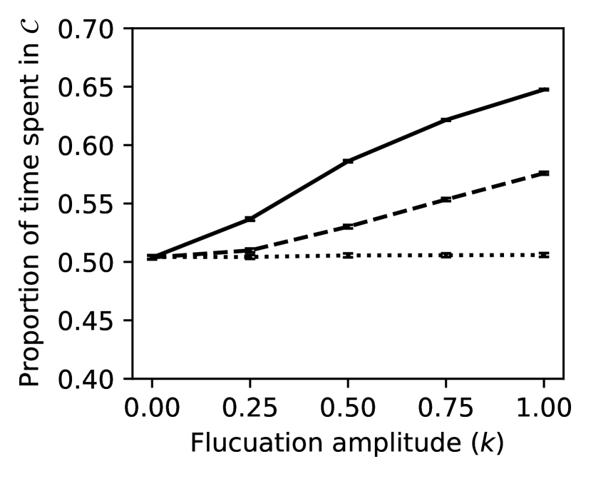
(a) Linear Intervention Cost

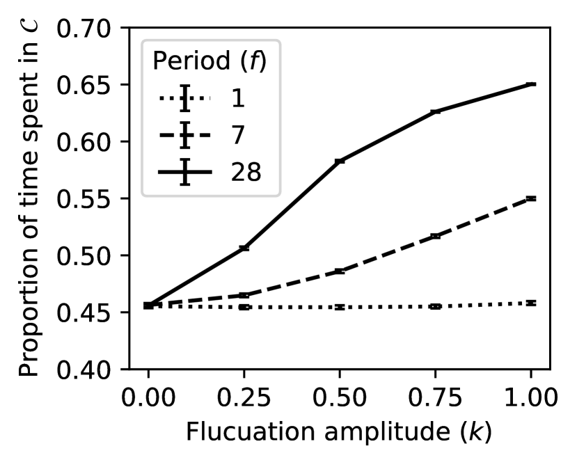
(b) Quadratic Intervention Cost

Figure 10: Long-run fraction of time with all servers busy under the fluid policy and for three periods and varying amplitudes. Other system parameters are $N=50,\bar{\lambda}=0.95,\mu=1/4,\nu=1/15$; and cost parameters are fixed at $r=1,M=0.5,h=1/4$ with $C(p)=5(0.2-p)$ (left) and quadratic $C(p)=50(0.2-p)^{2}$ (right).

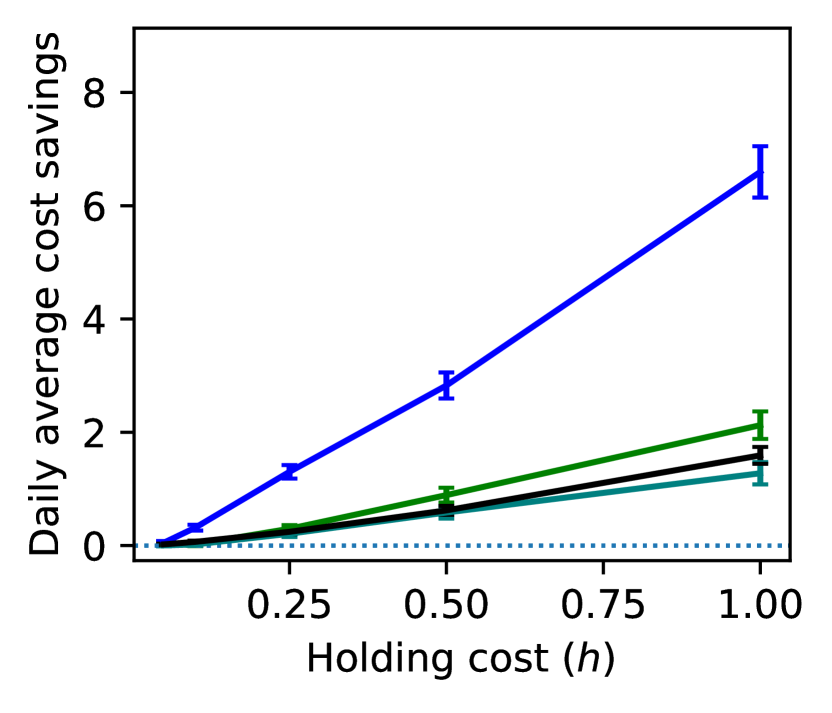
(a) $M=0.2$

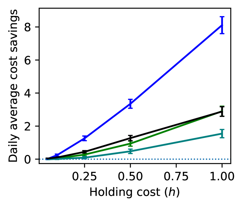
(b) $M=0.5$

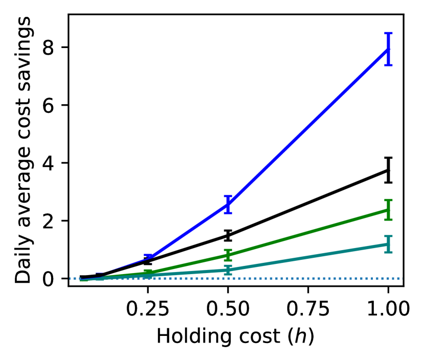
(c) $M=1.0$

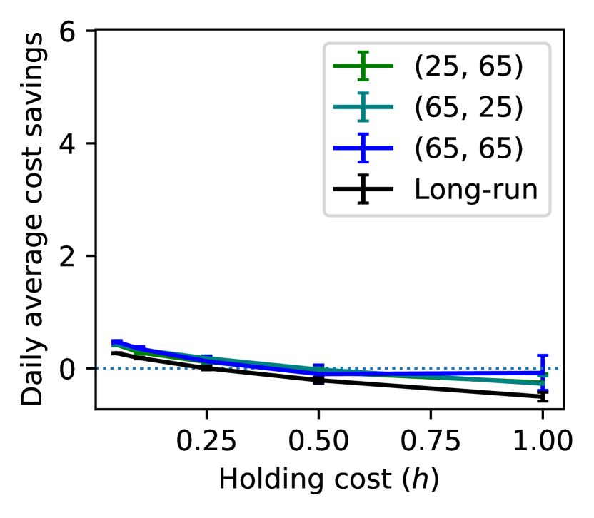
(d) $M=0.2$

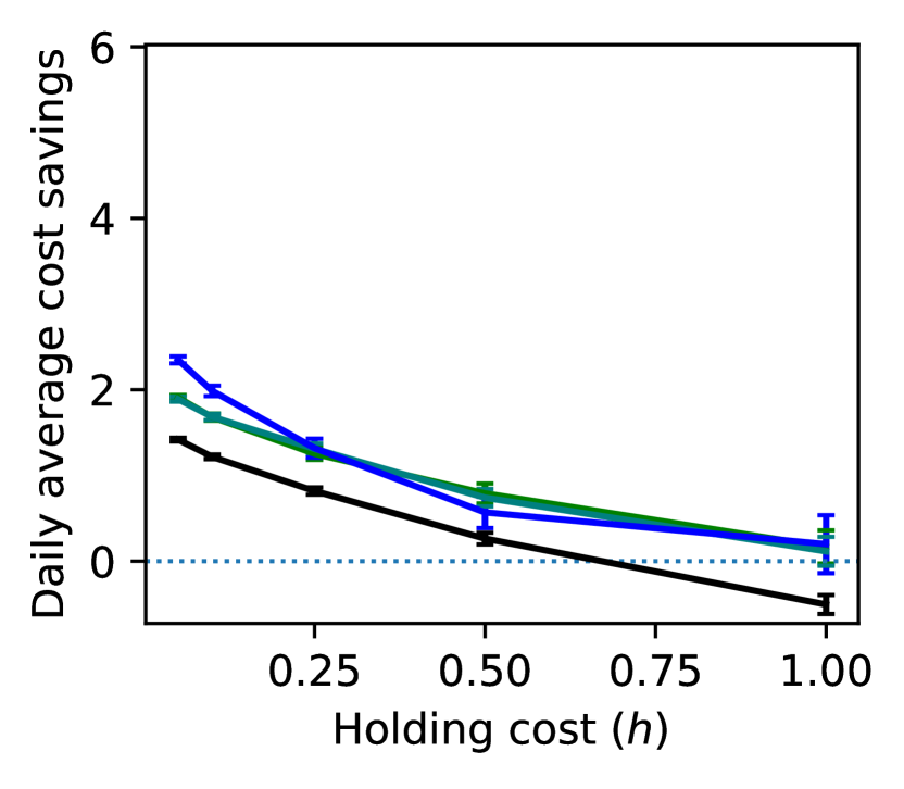
(e) $M=0.5$

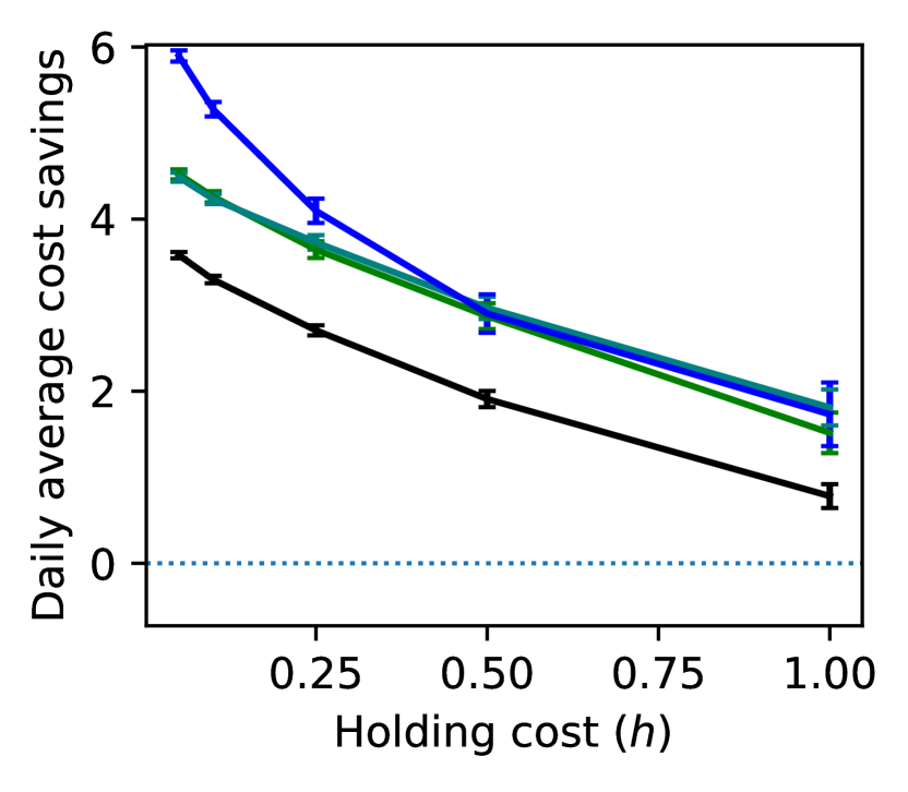
(f) $M=1.0$

Figure 11: Absolute reduction in expected cost for both finite-horizon and long-run experiments under the fluid policy with respect to the equilibrium policy (top row) and simple policy (bottom row) and under different values of cost parameters and the quadratic intervention cost. System parameters are fixed at $N=50,\lambda=0.9,\mu=1/4,\nu=1/15$ and and the return cost is normalized at $r=1$.

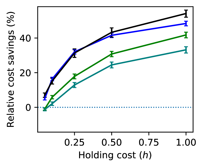
(a) $M=0.2$

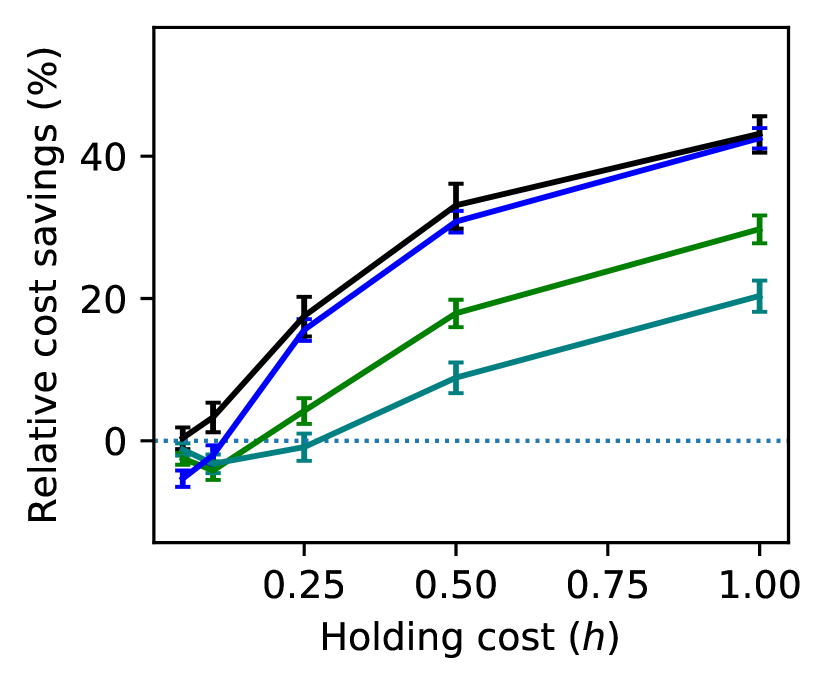
(b) $M=0.5$

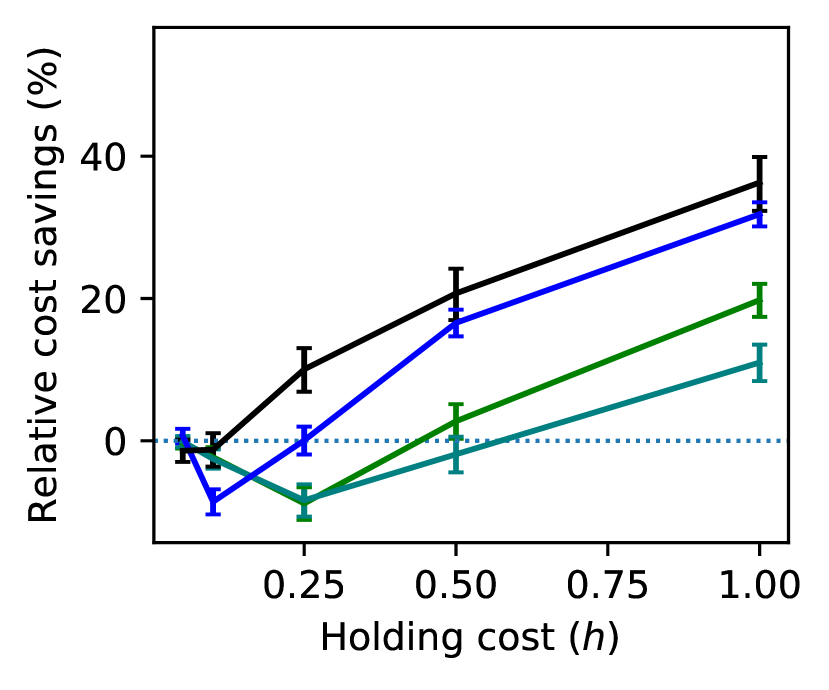
(c) $M=1.0$

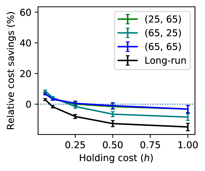
(d) $M=0.2$

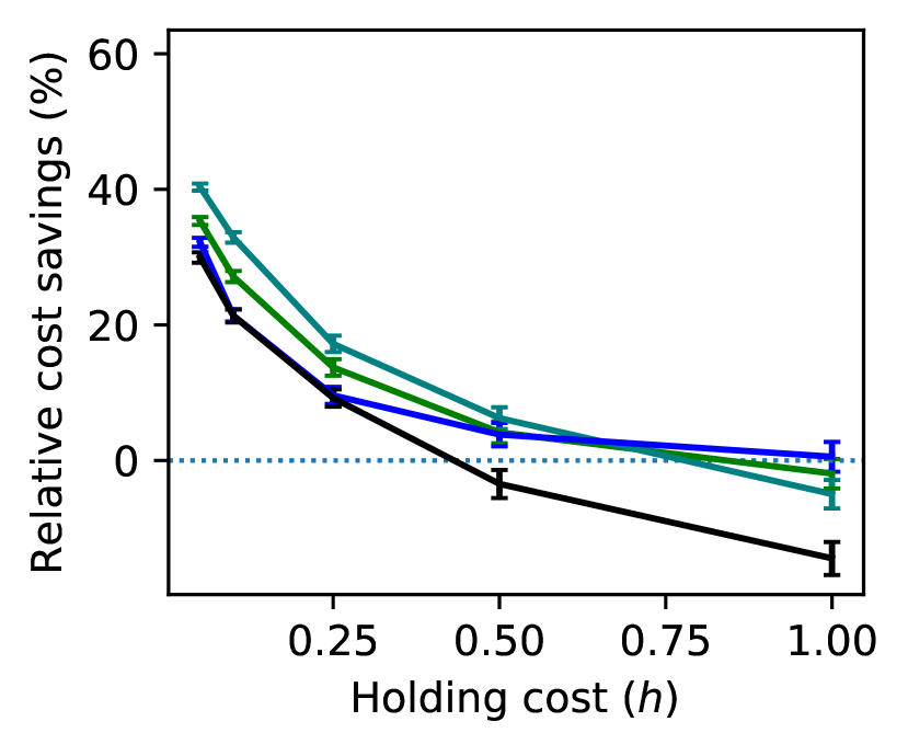
(e) $M=0.5$

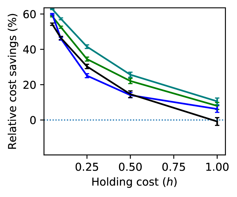
(f) $M=1.0$

Figure 12: Relative reduction in expected cost for both finite-horizon and long-run experiments under the fluid policy with respect to the equilibrium policy (top row) and simple policy (bottom row) under the linear intervention cost and for different values of cost parameters. System parameters are fixed at $N=50,\lambda=0.95,\mu=1/4,\nu=1/15$ and the return cost is normalized at $r=1$.

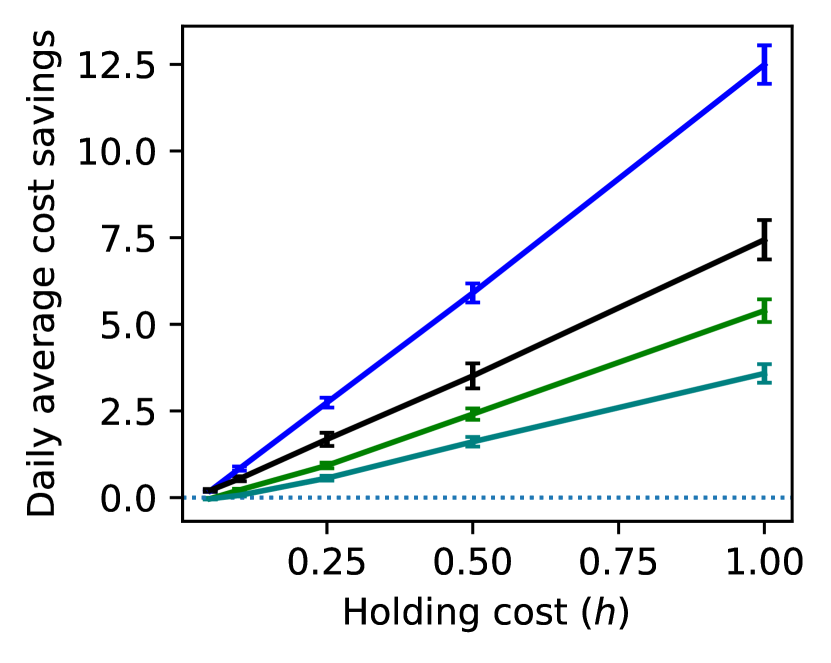
(a) $M=0.2$

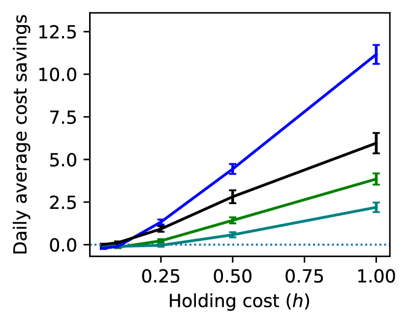
(b) $M=0.5$

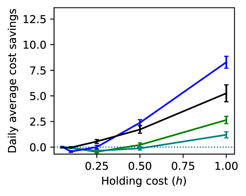
(c) $M=1.0$

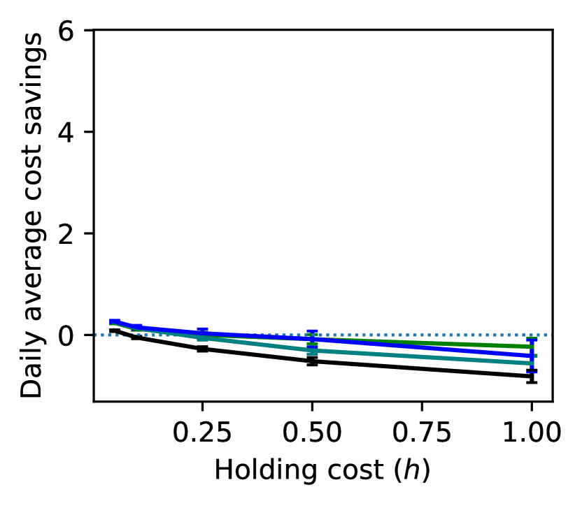
(d) $M=0.2$

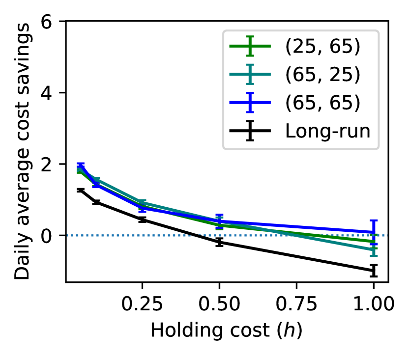
(e) $M=0.5$

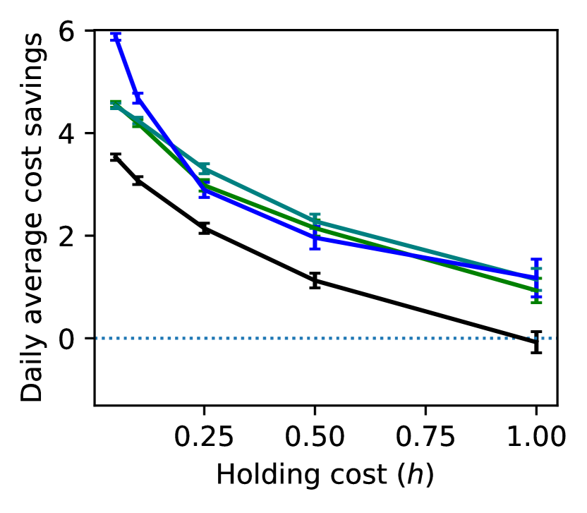
(f) $M=1.0$

Figure 13: Relative reduction in expected cost for both finite-horizon and long-run experiments under the fluid policy with respect to the equilibrium policy (top row) and simple policy (bottom row) and under different values of cost parameters and the linear intervention cost. System parameters are fixed at $N=50,\lambda=0.95,\mu=1/4,\nu=1/15$ and the return cost is normalized at $r=1$.

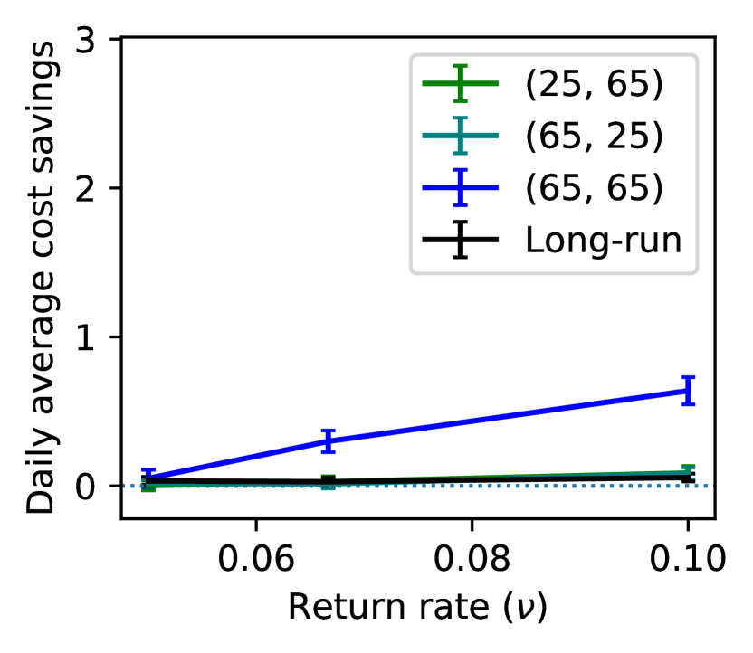
(a) $\lambda=9.0$

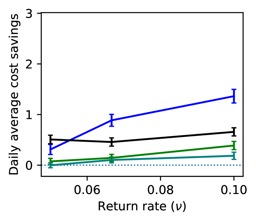
(b) $\lambda=9.5$

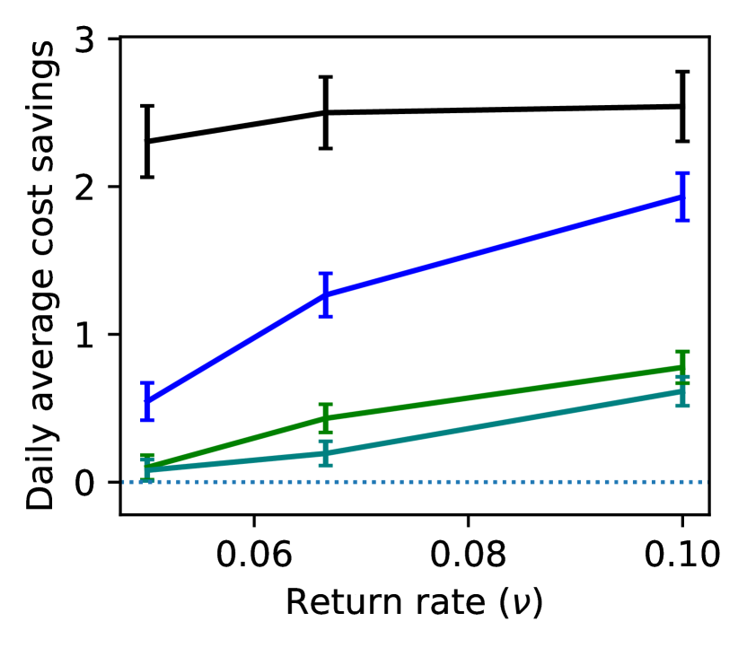
(c) $\lambda=9.8$

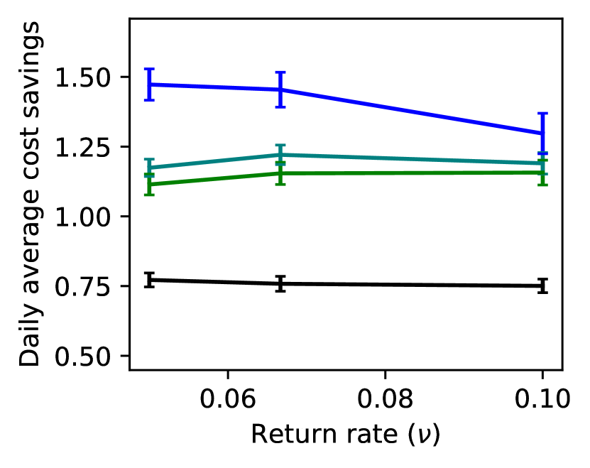
(d) $\lambda=9.0$

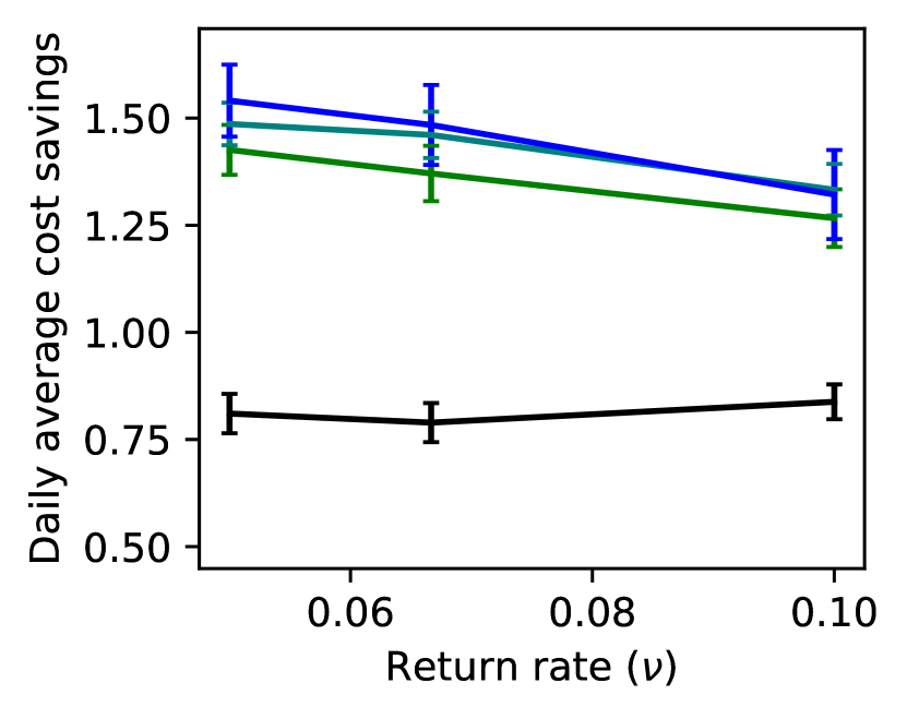
(e) $\lambda=9.5$

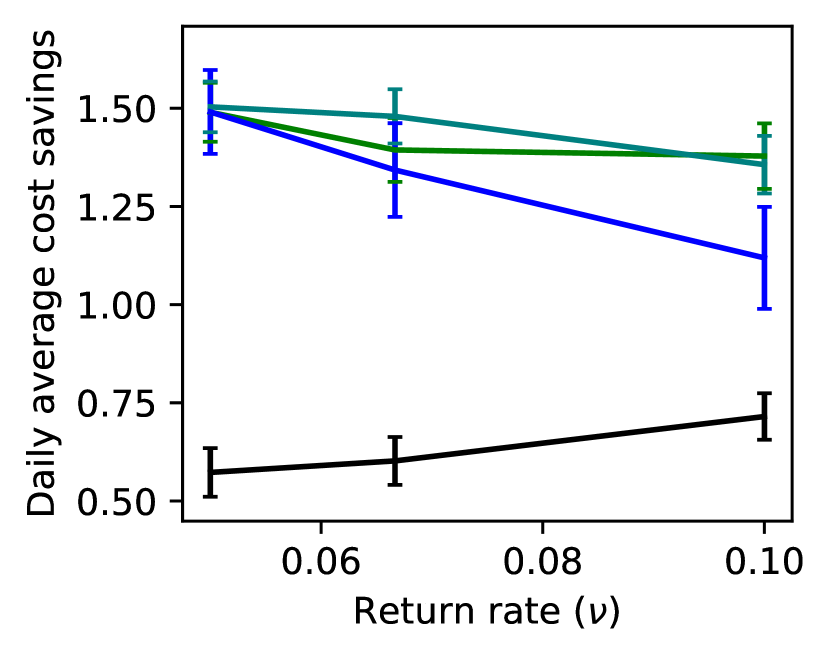
(f) $\lambda=9.8$

Figure 14: Absolute reduction in expected cost for both finite-horizon and long-run experiments under the fluid policy with respect to the equilibrium policy (top row) and simple policy (bottom row) under the quadratic intervention cost and for different values of arrival $\lambda$ and return $\nu$ rates. Other cost and system parameters are fixed at $N=50,\lambda=0.95,\mu=1/4,\nu=1/15,r=1,M=0.5,h=1/4$.

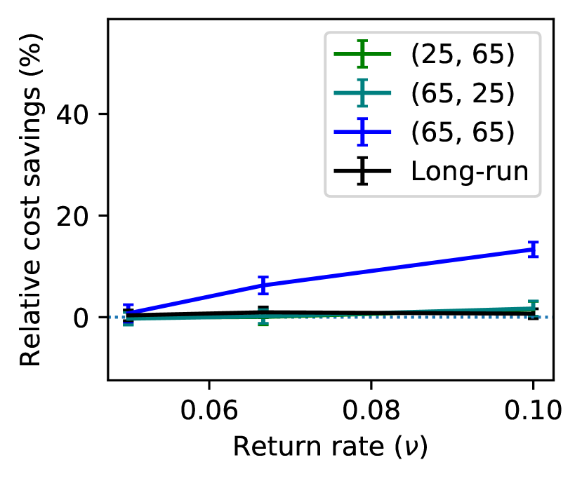
(a) $\lambda=9.0$

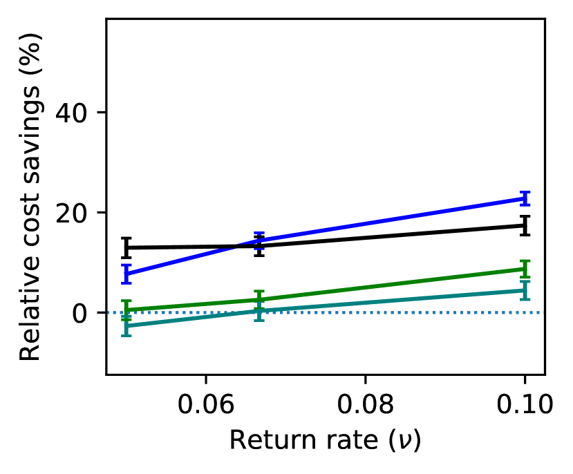
(b) $\lambda=9.5$

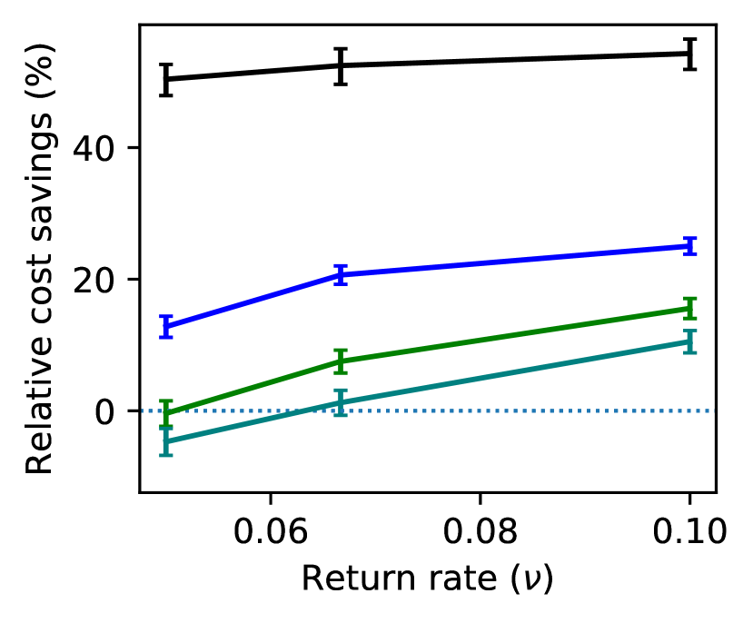
(c) $\lambda=9.8$

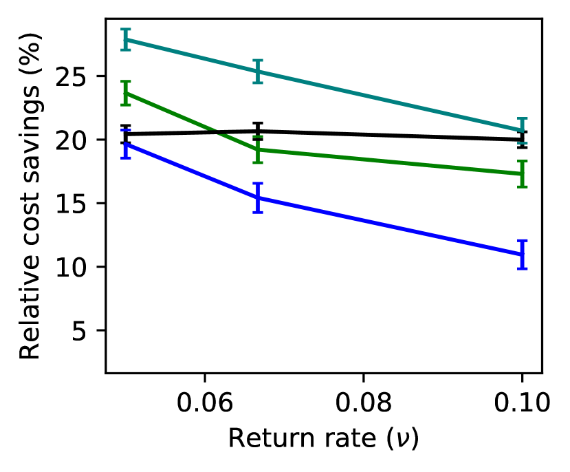
(d) $\lambda=9.0$

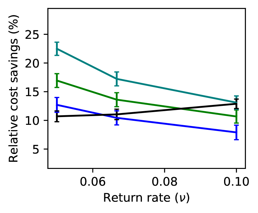
(e) $\lambda=9.5$

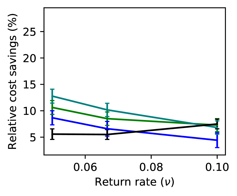
(f) $\lambda=9.8$

Figure 15: Relative reduction in expected cost for both finite-horizon and long-run experiments under the fluid policy with respect to the equilibrium policy (top row) and simple policy (bottom row) under the linear intervention cost and for different values of arrival $\lambda$ and return $\nu$ rates. Other cost and system parameters are fixed at $N=50,\mu=1/4,r=1,M=0.5,h=1/4$.

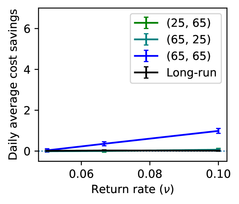
(a) $\lambda=9.0$

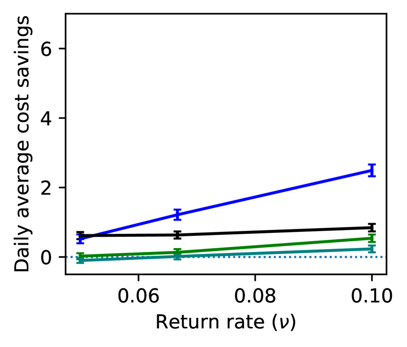
(b) $\lambda=9.5$

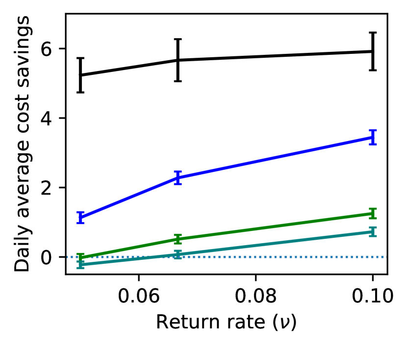
(c) $\lambda=9.8$

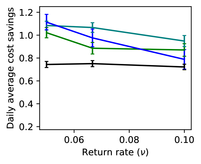
(d) $\lambda=9.0$

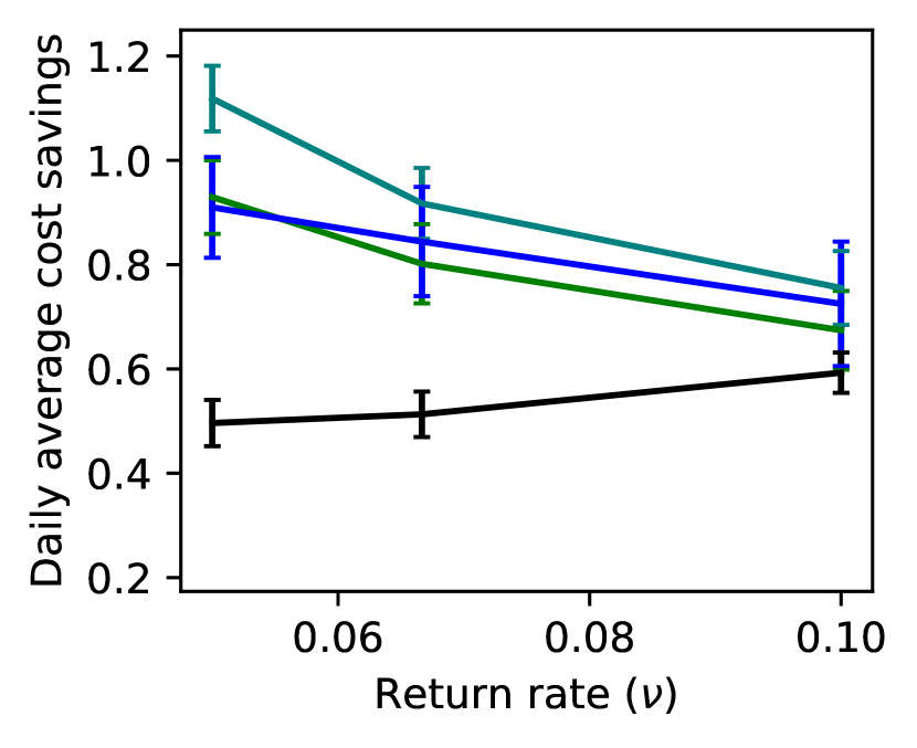
(e) $\lambda=9.5$

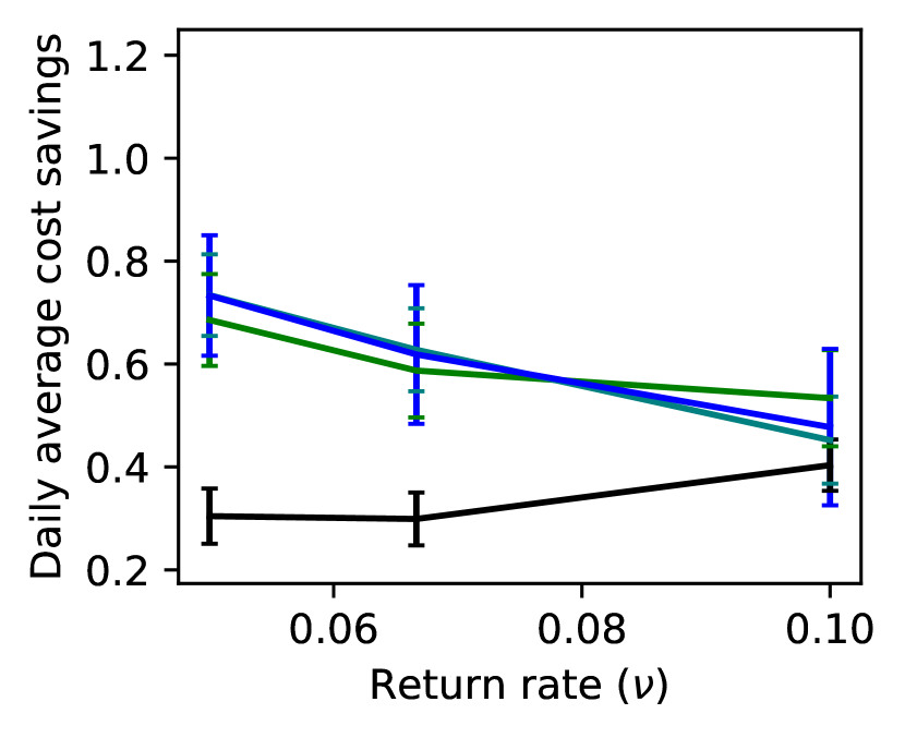
(f) $\lambda=9.8$

Figure 16: Absolute reduction in expected cost for both finite-horizon and long-run experiments under the fluid policy with respect to the equilibrium policy (top row) and simple policy (bottom row) under the linear intervention cost and for different values of arrival $\lambda$ and return $\nu$ rates. Other cost and system parameters are fixed at $N=50,\mu=1/4,r=1,M=0.5,h=1/4$.

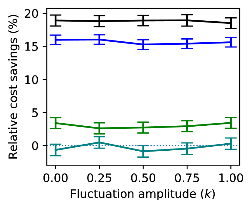
(a) $f=1$

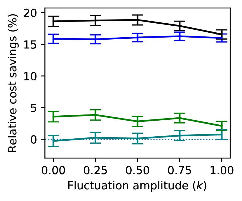
(b) $f=7$

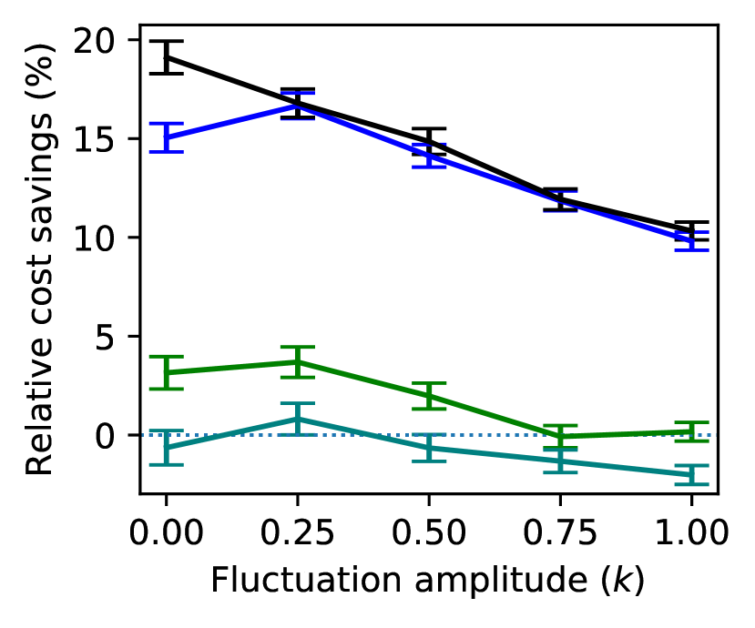
(c) $f=28$

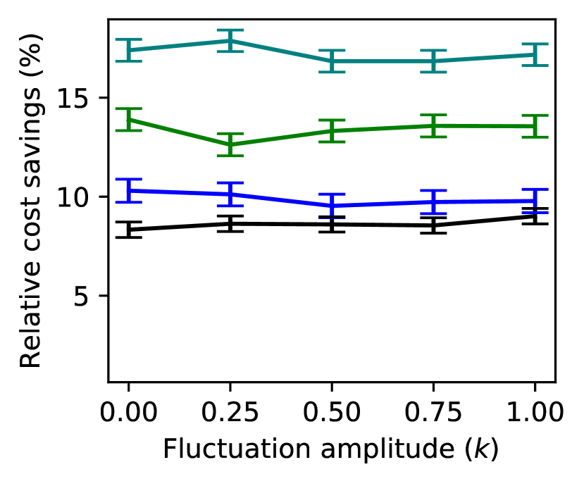
(d) $f=1$

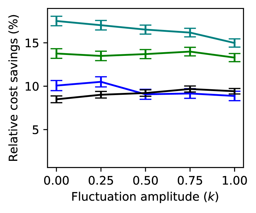
(e) $f=7$

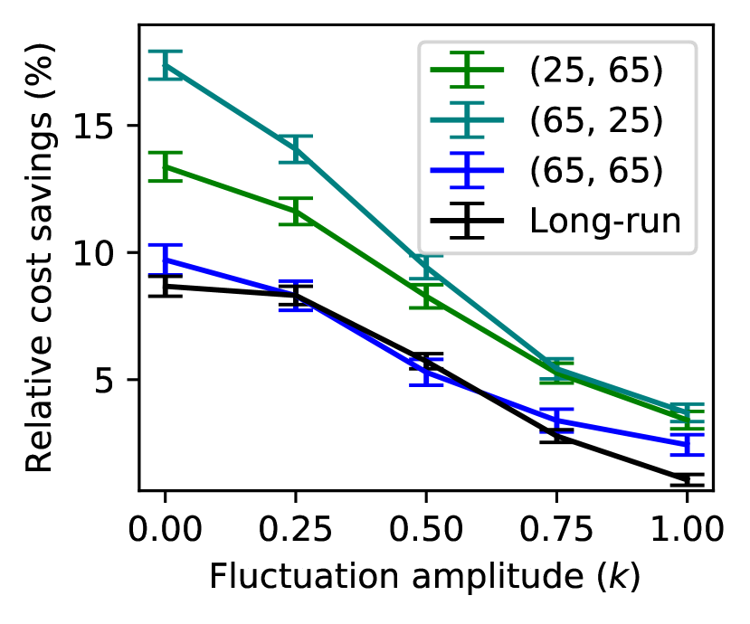
(f) $f=28$

Figure 17: Relative reduction in expected cost under the linear intervention cost for the fluid policy with respect to the equilibrium policy (top row) and simple policy (bottom row) and under different time-varying arrival rate functions. System and cost parameters are fixed at $N=50,\bar{\lambda}=0.95,\mu=1/4,\nu=1/15,r=1,h=1/4,C(p)=5(0.2-p)$.

References

- Arifoğlu et al. [2021] K. Arifoğlu, H. Ren, and T. Tezcan. Hospital readmissions reduction program does not provide the right incentives: Issues and remedies. Management Science, 67(4):2191–2210, 2021.
- Armony et al. [2015] M. Armony, S. Israelit, A. Mandelbaum, Y. N. Marmor, Y. Tseytlin, and G. B. Yom-Tov. On patient flow in hospitals: A data-based queueing-science perspective. Stochastic Systems, 5(1):146–194, 2015.
- Ata and Peng [2020] B. Ata and X. Peng. An optimal callback policy for general arrival processes: a pathwise analysis. Operations Research, 68(2):327–347, 2020.
- Avram et al. [1994] F. Avram, D. Bertsimas, and M. Richard. Stochastic networks. In Proceedings of the IMA, pages 199–234, 1994.
- Badaracco et al. [2021] N. Badaracco, M. Burns, and L. Dague. The effects of medicaid coverage on post-incarceration employment and recidivism. Health Services Research, 56:24–25, 2021.
- Barjesteh and Abouee-Mehrizi [2021] N. Barjesteh and H. Abouee-Mehrizi. Multiclass state-dependent service systems with returns. Naval Research Logistics (NRL), 68(5):631–662, 2021.
- Bayati et al. [2014] M. Bayati, M. Braverman, M. Gillam, K. M. Mack, G. Ruiz, M. S. Smith, and E. Horvitz. Data-driven decisions for reducing readmissions for heart failure: General methodology and case study. PloS one, 9(10):e109264, 2014.
- Bhulai et al. [2014] S. Bhulai, A. Brooms, and F. Spieksma. On structural properties of the value function for an unbounded jump markov process with an application to a processor sharing retrial queue. Queueing Systems, 76:425–446, 2014.
- Chan et al. [2014] C. W. Chan, G. Yom-Tov, and G. Escobar. When to use speedup: An examination of service systems with returns. Operations Research, 62(2):462–482, 2014.
- Chan et al. [2021] C. W. Chan, M. Huang, and V. Sarhangian. Dynamic server assignment in multiclass queues with shifts, with applications to nurse staffing in emergency departments. Operations Research, 2021.
- Down et al. [2011] D. G. Down, G. Koole, and M. E. Lewis. Dynamic control of a single-server system with abandonments. Queueing Systems, 67(1):63–90, 2011.
- Fieller [1932] E. C. Fieller. The distribution of the index in a normal bivariate population. Biometrika, 24(3/4):428–440, 1932.
- Green et al. [2007] L. V. Green, P. J. Kolesar, and W. Whitt. Coping with time-varying demand when setting staffing requirements for a service system. Production and Operations Management, 16(1):13–39, 2007.
- Haviv and Puterman [1998] M. Haviv and M. L. Puterman. Bias optimality in controlled queueing systems. Journal of Applied Probability, 35(1):136–150, 1998.
- Helm et al. [2016] J. E. Helm, A. Alaeddini, J. M. Stauffer, K. M. Bretthauer, and T. A. Skolarus. Reducing hospital readmissions by integrating empirical prediction with resource optimization. Production and Operations Management, 25(2):233–257, 2016.
- Hu et al. [2021] Y. Hu, C. W. Chan, and J. Dong. Optimal scheduling of proactive service with customer deterioration and improvement. Management Science, 2021.
- Ingolfsson et al. [2020] A. Ingolfsson, E. Almehdawe, A. Pedram, and M. Tran. Comparison of fluid approximations for service systems with state-dependent service rates and return probabilities. European Journal of Operational Research, 283(2):562–575, 2020.
- Kirk [1998] D. E. Kirk. Optimal Control Theory: An Introduction. Prentice-Hall, 1998.
- Larranaga et al. [2013] M. Larranaga, U. Ayesta, and I. M. Verloop. Dynamic fluid-based scheduling in a multi-class abandonment queue. Performance Evaluation, 70(10):841–858, 2013.
- Larrañaga et al. [2015] M. Larrañaga, U. Ayesta, and I. M. Verloop. Asymptotically optimal index policies for an abandonment queue with convex holding cost. Queuing Systems, 81(2):99–169, 2015.
- Leppin et al. [2014] A. L. Leppin, M. R. Gionfriddo, M. Kessler, J. P. Brito, F. S. Mair, K. Gallacher, Z. Wang, P. J. Erwin, T. Sylvester, K. Boehmer, et al. Preventing 30-day hospital readmissions: a systematic review and meta-analysis of randomized trials. JAMA internal medicine, 174(7):1095–1107, 2014.
- Lewis and Puterman [2002] M. E. Lewis and M. L. Puterman. Bias optimality. In Handbook of Markov decision processes, pages 89–111. Springer, 2002.
- Liu et al. [2018] X. Liu, M. Hu, J. E. Helm, M. S. Lavieri, and T. A. Skolarus. Missed opportunities in preventing hospital readmissions: Redesigning post-discharge checkup policies. Production and Operations Management, 27(12):2226–2250, 2018.
- Maglaras [2000] C. Maglaras. Discrete-review policies for scheduling stochastic networks: Trajectory tracking and fluid-scale asymptotic optimality. Annals of Applied Probability, pages 897–929, 2000.
- Maglaras [2006] C. Maglaras. Revenue management for a multiclass single-server queue via a fluid model analysis. Operations Research, 54(5):914–932, 2006.
- Mandelbaum et al. [1998] A. Mandelbaum, W. A. Massey, and M. I. Reiman. Strong approximations for markovian service networks. Queueing Systems, 30(1):149–201, 1998.
- Nuckols et al. [2017] T. K. Nuckols, E. Keeler, S. Morton, L. Anderson, B. J. Doyle, J. Pevnick, M. Booth, R. Shanman, A. Arifkhanova, and P. Shekelle. Economic evaluation of quality improvement interventions designed to prevent hospital readmission: a systematic review and meta-analysis. JAMA internal medicine, 177(7):975–985, 2017.
- Perry and Whitt [2009] O. Perry and W. Whitt. Responding to unexpected overloads in large-scale service systems. Management Science, 55(8):1353–1367, 2009.
- Ravn-Nielsen et al. [2018] L. V. Ravn-Nielsen, M.-L. Duckert, M. L. Lund, J. P. Henriksen, M. L. Nielsen, C. S. Eriksen, T. C. Buck, A. Pottegård, M. R. Hansen, and J. Hallas. Effect of an in-hospital multifaceted clinical pharmacist intervention on the risk of readmission: a randomized clinical trial. JAMA internal medicine, 178(3):375–382, 2018.
- Shi et al. [2021] P. Shi, J. E. Helm, J. Deglise-Hawkinson, and J. Pan. Timing it right: Balancing inpatient congestion vs. readmission risk at discharge. Operations Research, 2021.
- Stauffer et al. [2011] B. Stauffer, C. Fullerton, N. Fleming, G. Ogola, J. Herrin, P. Stafford, and D. Ballard. Effectiveness and cost of a transitional care program for heart failure: a prospective study with concurrent controls. Arch Intern Med, 171(14):1238–1243, 2011.
- Todorov [2006] E. Todorov. Optimal control theory. In K. Doya et al., editors, Bayesian Brain: Probabilistic Approaches to Neural Coding, chapter 12, pages 269–298. MIT Press, 2006.
- Usta and Wein [2015] M. Usta and L. M. Wein. Assessing risk-based policies for pretrial release and split sentencing in Los Angeles county jails. Plos One, 10(12):e0144967, 2015.
- Véricourt and Jennings [2011] F. d. Véricourt and O. B. Jennings. Nurse staffing in medical units: A queueing perspective. Operations Research, 59(6):1320–1331, 2011.
- Wallace [2015] D. Wallace. Do neighborhood organizational resources impact recidivism? Sociological Inquiry, 85(2):285–308, 2015.
- Yom-Tov and Mandelbaum [2014] G. B. Yom-Tov and A. Mandelbaum. Erlang-R: A time-varying queue with reentrant customers, in support of healthcare staffing. Manufacturing & Service Operations Management, 16(2):283–299, 2014.
- Zayas-Cabán et al. [2016] G. Zayas-Cabán, J. Xie, L. V. Green, and M. E. Lewis. Dynamic control of a tandem system with abandonments. Queueing Systems, 84(3):279–293, 2016.
- Zhang et al. [2016] D. J. Zhang, I. Gurvich, J. A. Van Mieghem, E. Park, R. S. Young, and M. V. Williams. Hospital readmissions reduction program: An economic and operational analysis. Management Science, 62(11):3351–3371, 2016.