Amortized Proximal Optimization

Abstract

We propose a framework for online meta-optimization of parameters that govern optimization, called Amortized Proximal Optimization (APO). We first interpret various existing neural network optimizers as approximate stochastic proximal point methods which trade off the current-batch loss with proximity terms in both function space and weight space. The idea behind APO is to amortize the minimization of the proximal point objective by meta-learning the parameters of an update rule. We show how APO can be used to adapt a learning rate or a structured preconditioning matrix. Under appropriate assumptions, APO can recover existing optimizers such as natural gradient descent and KFAC. It enjoys low computational overhead and avoids expensive and numerically sensitive operations required by some second-order optimizers, such as matrix inverses. We empirically test APO for online adaptation of learning rates and structured preconditioning matrices for regression, image reconstruction, image classification, and natural language translation tasks. Empirically, the learning rate schedules found by APO generally outperform optimal fixed learning rates and are competitive with manually tuned decay schedules. Using APO to adapt a structured preconditioning matrix generally results in optimization performance competitive with second-order methods. Moreover, the absence of matrix inversion provides numerical stability, making it effective for low precision training.

1 Introduction

Many optimization algorithms widely used in machine learning can be seen as approximations to an idealized algorithm called the proximal point method (PPM). When training neural networks, the stochastic PPM iteratively minimizes a loss function $\mathcal{J}_{\mathcal{B}}\colon\mathbb{R}^{m}\to\mathbb{R}$ on a mini-batch $\mathcal{B}$, plus a proximity term that penalizes the discrepancy from the current iterate:

$${\bm{\theta}}^{(t+1)}\leftarrow\operatorname*{arg\,min}_{\mathbf{u}\in\mathbb{R}^{m}}\mathcal{J}_{\mathcal{B}^{(t)}}(\mathbf{u})+\lambda D(\mathbf{u},{\bm{\theta}}^{(t)}),$$ (1)

where $D(\cdot,\cdot)$ measures the discrepancy between two vectors and $\lambda>0$ is a hyperparameter that controls the strength of the proximity term. The proximity term discourages the update from excessively changing the parameters, hence preventing aggressive updates. Moreover, the stochastic PPM has good convergence properties (Asi & Duchi, 2019). While minimizing Eq. 1 exactly is usually impractical (or at least uneconomical), solving it approximately (by taking first or second-order Taylor series approximations to the loss or the proximity term) has motivated important and widely used optimization algorithms such as natural gradient descent (Amari, 1998) and mirror descent (Beck & Teboulle, 2003). Stochastic gradient descent (SGD) (Robbins & Monro, 1951) itself can be seen as an approximate PPM where the loss term is linearized and the discrepancy function is squared Euclidean distance.

Inspired by the idea that the PPM is a useful algorithm to approximate, we propose to amortize the minimization of Eq. 1 by defining a parametric form for an update rule which is likely to be good at minimizing it and adapting its parameters with gradient-based optimization. We consider adapting optimization hyperparameters (such as the learning rate) for existing optimizers such as SGD and RMSprop (Tieleman & Hinton, 2012), as well as learning structured preconditioning matrices. By choosing a structure for the update rule inspired by existing optimizers, we can take advantage of the insights that went into those optimizers while still being robust to cases where their assumptions (such as the use of linear or quadratic approximations) break down. By doing meta-descent on the optimization parameters, we can amortize the cost of minimizing the PPM objective, which would otherwise take many steps per parameter update. Hence, we call our approach Amortized Proximal Optimization (APO).

Eq. 1 leaves a lot of freedom for the proximity term. We argue that many of the most effective neural network optimizers can be seen as trading off two different proximity terms: a function space discrepancy (FSD) term which penalizes the average change to the network’s predictions, and a weight space discrepancy (WSD) term which prevents the weights from moving too far, hence encouraging smoothness to the update and maintaining the accuracy of second-order approximations. Our meta-objective includes both terms.

Our formulation of APO is general, and can be applied to various settings, from optimizing a single optimization hyperparameter to learning a flexible update rule. We consider two use cases that cover both ends of this spectrum. At one end, we consider the problem of adapting learning rates of existing optimizers, specifically SGD, RMSprop, and Adam (Duchi et al., 2011). The learning rate is considered one of the most essential hyperparameters to tune (Bengio, 2012), and good learning rate schedules are often found by years of trial and error. Empirically, the learning rates found by APO outperformed the best fixed learning rates and were competitive with manual step decay schedules.

Our second use case is more ambitious. We use APO to learn a preconditioning matrix, giving the update rule the flexibility to represent second-order optimization updates such as Newton’s method, Gauss-Newton, or natural gradient descent. We show that, under certain conditions, the optimum of our APO meta-objective with respect to a full preconditioning matrix coincides with damped versions of natural gradient descent or Gauss-Newton. While computing and storing a full preconditioning matrix for a large neural network is impractical, various practical approximations have been developed. We use APO to meta-learn a structured preconditioning matrix based on the EKFAC optimizer (George et al., 2018). APO is more straightforward to implement in current-day deep learning frameworks than EKFAC and is also more computationally efficient per iteration because it avoids the need to compute eigendecompositions. Empirically, we evaluate APO for learning structured preconditioners on regression, image reconstruction, image classification, and neural machine translation tasks. The preconditioning matrix adapted by APO achieved competitive convergence to other second-order optimizers.

2 Preliminaries

Consider a prediction problem from some input space $\mathcal{X}$ to an output space $\mathcal{T}$. We are given a finite training set $\mathcal{D}_{\text{train}}=\{(\mathbf{x}^{(i)},\mathbf{t}^{(i)})\}^{N}_{i=1}$. For a data point $(\mathbf{x},\mathbf{t})$ and parameters ${\bm{\theta}}\in\mathbb{R}^{m}$, let $\mathbf{y}=f(\mathbf{x},{\bm{\theta}})$ be the prediction of a network parameterized by ${\bm{\theta}}$ and $\mathcal{L}(\mathbf{y},\mathbf{t})$ be the loss. Our goal is to minimize the cost function:

$$\mathcal{J}({\bm{\theta}})=\frac{1}{N}\sum_{i=1}^{N}\mathcal{L}(f(\mathbf{x}^{(i)},{\bm{\theta}}),\mathbf{t}^{(i)}).$$ (2)

We use $\mathcal{J}_{\mathcal{B}}({\bm{\theta}})$ to denote the mean loss on a mini-batch of examples $\mathcal{B}=\{(\mathbf{x}^{(i)},\mathbf{t}^{(i)})\}_{i=1}^{B}$. We summarize the notation used in this paper in Appendix A.

3 Proximal Optimization and Second-Order Methods:
A Unifying Framework

We first motivate the proximal objective that we use as the meta-objective for APO, and relate it to existing neural network optimization methods. Our framework is largely based on Grosse (2021), to which readers are referred for a more detailed discussion.

3.1 Proximal Optimization

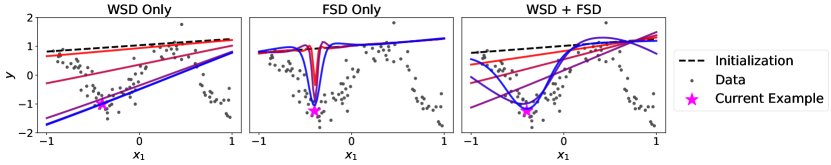
Figure 1: 1D illustration of the exact proximal update on a regression problem with a batch size of 1, taking inspiration from Grosse (2021). The weight of the discrepancy term(s) ($\lambda_{\text{WSD}}$ and $\lambda_{\text{FSD}}$) is decreased from red to blue.

When we update the parameters on a mini-batch of data, we would like to reduce the loss on that mini-batch, while not changing the predictions on previously visited examples or moving too far in weight space. This motivates the following proximal point update:

$${\bm{\theta}}^{(t+1)}\leftarrow\operatorname*{arg\,min}_{\mathbf{u}\in\mathbb{R}^{m}}\mathcal{J}_{\mathcal{B}^{(t)}}(\mathbf{u}) +\lambda_{\text{FSD}}\mathbb{E}_{\tilde{\mathbf{x}}\sim\mathcal{D}}[D_{\text{F}}(\mathbf{u},{\bm{\theta}}^{(t)},\tilde{\mathbf{x}})]+\lambda_{\text{WSD}}D_{\text{W}}({\mathbf{u},{\bm{\theta}}^{(t)}}),$$ (3)

where $D_{\text{F}}(\mathbf{u},{\bm{\theta}},\mathbf{x})=\rho(f(\mathbf{x},\mathbf{u}),f(\mathbf{x},\bm{\theta}))$ and $D_{\text{W}}(\mathbf{u},{\bm{\theta}})=\nicefrac{{1}}{{2}}\|\mathbf{u}-{\bm{\theta}}\|^{2}_{2}$ are discrepancy functions, described in detail below. Here, $\lambda_{\text{FSD}}$ and $\lambda_{\text{WSD}}$ are hyperparameters that control the strength of each discrepancy term, $\tilde{\mathbf{x}}$ is a random data point sampled from the data-generating distribution $\mathcal{D}$, and $\rho(\cdot,\cdot)$ is the output-space divergence.

The proximal objective in Eq. 3 consists of three terms. The first term is the loss on the current mini-batch. The second term is the function space discrepancy (FSD), whose role is to prevent the update from substantially altering the predictions on other data points. The general idea of the FSD term has been successful in alleviating catastrophic forgetting (Benjamin et al., 2018), fine-tuning pre-trained models (Jiang et al., 2019), and training a student model from a teacher network (Hinton et al., 2015).

The final term is the weight space discrepancy (WSD); this term encourages the update to move the parameters as little as possible. It can be used to motivate damping in the context of second-order optimization (Martens, 2016). While weight space distance may appear counterproductive from an optimization standpoint because it depends on the model parameterization, modern analyses of neural network optimization and generalization often rely on neural network parameters staying close to their initialization in the Euclidean norm (Jacot et al., 2018; Zhang et al., 2019b; Belkin et al., 2019). In fact, Wadia et al. (2021) showed that pure second-order optimizers (i.e. ones without some form of WSD regularization) are unable to generalize in the overparameterized setting.

Figure 1 illustrates the effects of the WSD and FSD terms on the exact PPM update for a 1D regression example with a batch size of 1. If the proximal objective includes only the loss and WSD term (i.e. $\lambda_{\text{FSD}}=0$), the PPM update makes the minimal change to the weights which fits the current example, resulting in a global adjustment to the function which overwrites all the other predictions. If only the loss and FSD terms are used (i.e. $\lambda_{\text{WSD}}=0$), the update carves a spike around the current data point, failing to improve predictions on nearby examples and running the risk of memorization. When both WSD and FSD are penalized, it makes a local adjustment to the predictions, but one which nonetheless improves performance on nearby examples.

3.2 Connection Between Proximal Optimization and Second-Order Optimization

Method	Loss Approx.	FSD	WSD
Gradient Descent	$1^{\text{st}}$-order	-	✓
Hessian-Free	$2^{\text{nd}}$-order	-	✓
Natural Gradient	$1^{\text{st}}$-order	$2^{\text{nd}}$-order	✗
Proximal Point	Exact	Exact	✓

Table 1: Various classical first- and second-order optimization algorithms can be interpreted as minimizing approximations of the proximal objective in Eq. 3, using 1${}^{\text{st}}$ or 2${}^{\text{nd}}$ order Taylor expansions of the loss or FSD terms.

We further motivate our proximal objective by relating it to existing neural network optimizers. Ordinary SGD can be viewed as an approximate PPM update with a first-order approximation to the loss term and no FSD term. Hessian-free optimization (Martens, 2010), a classic second-order optimization method for neural networks, approximately minimizes a second-order approximation to the loss on each batch using conjugate gradients. It can be seen as minimizing a quadratic approximation to Eq. 3 with no FSD term.

Amari (1998) motivated natural gradient descent (NGD) as a steepest descent method with an infinitesimal step size; this justifies a first-order approximation to the loss term and a second-order approximation to the proximity term. Optimizing over a manifold of probability distributions with KL divergence as the proximity term yields the familiar update involving the Fisher information matrix. Natural gradient optimization of neural networks (Martens, 2014; Martens & Grosse, 2015) can be interpreted as minimizing Eq. 3 with a linear approximation to the loss term and a quadratic approximation to the FSD term. While NGD traditionally omits the WSD term in order to achieve parameterization invariance, it is typically included in practical neural network optimizers for stability (Martens & Grosse, 2015).

In a more general context, when taking a first-order approximation to the loss and a second-order approximation to the FSD, the update rule is given in closed form as:

$${\bm{\theta}}^{(t+1)}\approx{\bm{\theta}}^{(t)}-(\lambda_{\text{FSD}}\mathbf{G}+\lambda_{\text{WSD}}\mathbf{I})^{-1}\nabla_{{\bm{\theta}}}\mathcal{J}_{\mathcal{B}}({\bm{\theta}}^{(t)}),$$ (4)

where $\mathbf{G}$ is the Hessian of the FSD term. The derivation is shown in Appendix E. All of these relationships are summarized in Table 1, and derivations of all of these claims are given in Appendix F.

4 Amortized Proximal Optimization

In this section, we introduce Amortized Proximal Optimization (APO), an approach for online meta-learning of optimization parameters. Then, we describe two use cases that we explore in the paper: (1) adapting learning rates of existing base optimizers such as SGD, RMSProp, and Adam, and (2) meta-learning a structured preconditioning matrix.

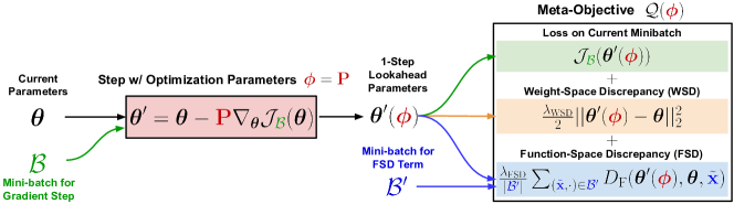
Figure 2: Amortized Proximal Optimization (APO). In each meta-optimization step, we perform a one-step lookahead from the current parameters $\bm{\theta}$ to obtain updated parameters $\bm{\theta}^{\prime}({\color[rgb]{0.8,0.0,0}\bm{\phi}})$, where ${\color[rgb]{0.8,0.0,0}\bm{\phi}}$ denotes the optimization parameters (e.g. learning rate ${\color[rgb]{0.8,0.0,0}\eta}$ or preconditioner ${\color[rgb]{0.8,0.0,0}\mathbf{P}}$). The meta-objective $\mathcal{Q}({\color[rgb]{0.8,0.0,0}\bm{\phi}})$ then evaluates the proximal point objective at $\bm{\theta}^{\prime}({\color[rgb]{0.8,0.0,0}\bm{\phi}})$. Note that the loss term in $\mathcal{Q}({\color[rgb]{0.8,0.0,0}\bm{\phi}})$ is computed on the same data that was used to compute the gradient for the lookahead step, ${\color[rgb]{0,0.6,0}\mathcal{B}}$, while the FSD term is computed using a different batch ${\color[rgb]{0.0,0.0,0.9}\mathcal{B}^{\prime}}$. The optimization parameters ${\color[rgb]{0.8,0.0,0}\bm{\phi}}$ are updated via the meta-gradient $\nabla_{{\color[rgb]{0.8,0.0,0}\bm{\phi}}}\mathcal{Q}({\color[rgb]{0.8,0.0,0}\bm{\phi}})$.

Algorithm 1 Amortized Proximal Optimization (APO) — Meta-Learning the Optimization Parameters ${\color[rgb]{1,0,0}\bm{\phi}}$

Require: $\bm{\theta}$ (initial model parameters), $\bm{\phi}$ (initial optimization parameters), $K$ (meta-update interval), $\alpha$ (meta-LR)

Require: $\lambda_{\text{WSD}}$ (weight-space discrepancy term weighting), $\lambda_{\text{FSD}}$ (function-space discrepancy term weighting)

while not converged, iteration $t$ do

     ${\color[rgb]{0,0.6,0}\mathcal{B}}\sim\mathcal{D}_{\text{train}}$ $\triangleright$ Sample mini-batch to compute the gradient and loss term

     if  $t\mod K=0$  then $\triangleright$ Perform meta-update every $K$ iterations

         ${\color[rgb]{0.0,0.0,0.9}\mathcal{B}^{\prime}}\sim\mathcal{D}_{\text{train}}$ $\triangleright$ Sample additional mini-batch to compute the FSD term

         $\bm{\theta}^{\prime}({\color[rgb]{0.8,0.0,0}\bm{\phi}}):=u({\bm{\theta}},{\color[rgb]{0.8,0.0,0}\bm{\phi}},{\color[rgb]{0,0.6,0}\mathcal{B}})$ $\triangleright$ Compute the 1-step lookahead parameters

         $\mathcal{Q}({\color[rgb]{0.8,0.0,0}\bm{\phi}}):=\mathcal{J}_{{\color[rgb]{0,0.6,0}\mathcal{B}}}\left(\bm{\theta}^{\prime}({\color[rgb]{0.8,0.0,0}\bm{\phi}}\right))+\nicefrac{{\lambda_{\text{FSD}}}}{{|{\color[rgb]{0.0,0.0,0.9}\mathcal{B}^{\prime}}|}}\sum_{({\color[rgb]{0.0,0.0,0.9}\tilde{\mathbf{x}}},\cdot)\in{\color[rgb]{0.0,0.0,0.9}\mathcal{B}^{\prime}}}D_{\text{F}}(\bm{\theta}^{\prime}({\color[rgb]{0.8,0.0,0}\bm{\phi}}),\bm{\theta},{\color[rgb]{0.0,0.0,0.9}\tilde{\mathbf{x}}})+\nicefrac{{\lambda_{\text{WSD}}}}{{2}}\left\lVert\bm{\theta}^{\prime}({\color[rgb]{0.8,0.0,0}\bm{\phi}})-\bm{\theta}\right\rVert^{2}_{2}$ $\triangleright$ Meta-objective

         ${\color[rgb]{0.8,0.0,0}\bm{\phi}}\leftarrow{\color[rgb]{0.8,0.0,0}\bm{\phi}}-\alpha\nabla_{{\color[rgb]{0.8,0.0,0}\bm{\phi}}}\mathcal{Q}({\color[rgb]{0.8,0.0,0}\bm{\phi}})$ $\triangleright$ Update optimizer parameters (e.g. LR or preconditioner)

     end if

     $\bm{\theta}\leftarrow u(\bm{\theta},{\color[rgb]{0.8,0.0,0}\bm{\phi}},{\color[rgb]{0,0.6,0}\mathcal{B}})$ $\triangleright$ Update model parameters

end while

4.1 Proximal Meta-Optimization

We assume an update rule $u$ parameterized by a vector $\bm{\phi}$ which updates the network weights ${\bm{\theta}}$ on a batch $\mathcal{B}^{(t)}$:

$${\bm{\theta}}^{(t+1)}\leftarrow u({\bm{\theta}}^{(t)},\bm{\phi},\mathcal{B}^{(t)}),$$ (5)

One use case of APO is to tune the hyperparameters of an existing optimizer, in which case $\bm{\phi}$ denotes the hyperparameters. For example, when tuning the SGD learning rate, we have $\bm{\phi}=\eta$ and the update is given by:

$$u_{\text{SGD}}({\bm{\theta}},\eta,\mathcal{B}) ={\bm{\theta}}-\eta\nabla_{{\bm{\theta}}}\mathcal{J}_{\mathcal{B}}({\bm{\theta}}).$$ (6)

More ambitiously, we could use APO to adapt a full preconditioning matrix $\mathbf{P}$. In this case, we define $\bm{\phi}=\mathbf{P}$ and the update is given by:

$$u_{\text{Precond}}({\bm{\theta}},\mathbf{P},\mathcal{B}) ={\bm{\theta}}-\mathbf{P}\nabla_{{\bm{\theta}}}\mathcal{J}_{\mathcal{B}}({\bm{\theta}}).$$ (7)

In Section 3, we introduced a general proximal objective for training neural networks and observed that many optimization techniques could be seen as an approximation of PPM. Motivated by this connection, we propose to directly minimize the proximal objective with respect to the optimization parameters. While still being able to take advantage of valuable properties of existing optimizers, direct minimization can be robust to cases when the assumptions (such as linear and quadratic approximation of the cost) do not hold. Another advantage of adapting a parametric update rule is that we can amortize the cost of minimizing the proximal objective throughout training.

We propose to use the following meta-objective, which evaluates the proximal objective at $u(\bm{\theta},\bm{\phi},\mathcal{B})$:

$$\mathcal{Q}(\bm{\phi})= \mathbb{E}_{\mathcal{B}\sim\mathcal{D}}\Big{[}\mathcal{J}_{\mathcal{B}}(u(\bm{\theta},\bm{\phi},\mathcal{B}))+\lambda_{\text{FSD}}\mathbb{E}_{(\tilde{\mathbf{x}},\cdot)\sim\mathcal{D}}\left[D_{\text{F}}(u(\bm{\theta},\bm{\phi},\mathcal{B}),{\bm{\theta}},\tilde{\mathbf{x}})\right]+\frac{\lambda_{\text{WSD}}}{2}\|u(\bm{\theta},\bm{\phi},\mathcal{B})-{\bm{\theta}}\|^{2}\Big{]}.$$ (8)

In practice, we estimate the expectations in the meta-objective by sampling two different mini-batches, $\mathcal{B}$ and $\mathcal{B}^{\prime}$, where $\mathcal{B}$ is used to compute the gradient and the loss term, and $\mathcal{B}^{\prime}$ is used to compute the FSD term. Intuitively, this proximal meta-objective aims to find optimizer parameters $\bm{\phi}$ that minimize the loss on the current mini-batch, while constraining the size of the step with the FSD and WSD terms so that it does not overfit the current mini-batch and undo progress that has been made by other mini-batches.

The optimization parameters $\bm{\phi}$ are optimized with a stochastic gradient-based algorithm (the meta-optimizer). The meta-gradient $\nabla_{\bm{\phi}}\mathcal{Q}(\bm{\phi})$ can be computed via automatic differentiation through the one-step unrolled computation graph (see Figure 2). We refer to our framework as Amortized Proximal Optimization (APO). An overview of APO is provided in Algorithm 1.

4.2 APO for Learning Rate Adaptation

One use case of APO is to adapt the learning rate of an existing base optimizer such as SGD. To do so, we let $u_{\text{SGD}}({\bm{\theta}},\eta,\mathcal{B})$ be the 1-step lookahead of parameters and minimize the proximal meta-objective with respect to the learning rate $\eta$. Although adaptive optimizers such as RMSProp and Adam use coordinate-wise adaptive learning rates, they still have a global learning rate parameter which is essential to tune. APO can be applied to such global learning rates to find learning rate schedules (that depend on $\lambda_{\text{FSD}}$ or $\lambda_{\text{WSD}}$).

4.3 APO for Adaptive Preconditioning

More ambitiously, we can use the APO framework to adapt the preconditioning matrix, allowing the update rule to flexibly represent various second-order optimization updates. We let $u_{\text{Precond}}({\bm{\theta}},\mathbf{P},\mathcal{B})$ denote the parameters after 1 preconditioned gradient step and adapt the preconditioning matrix $\mathbf{P}$ according to our framework.

If the assumptions made when deriving the second-order methods (detailed in Section 3.2) hold, then the optimal preconditioning matrix of the proximal meta-objective can be equivalent to various second-order updates, depending on the choice of the FSD function.

Theorem 1.

Consider an approximation $\hat{\mathcal{Q}}(\mathbf{P})$ to the meta-objective (Eq. 8) where the loss term is linearized around the current weights $\bm{\theta}$ and the FSD term is replaced by its second-order approximation around $\bm{\theta}$. Denote the gradient on a mini-batch as $\mathbf{g}=\nabla_{\bm{\theta}}\mathcal{J}_{\mathcal{B}}(\bm{\theta})$, and assume that the second moment matrix $\mathbb{E}_{\mathcal{B}\sim\mathcal{D}}\left[\mathbf{g}\mathbf{g}^{\top}\right]$ is non-singular. Then, the preconditioning matrix which minimizes $\hat{\mathcal{Q}}$ is given by $\mathbf{P}^{\star}=(\lambda_{\text{FSD}}\mathbf{G}+\lambda_{\text{WSD}}\mathbf{I})^{-1}$, where $\mathbf{G}$ denotes the Hessian of the FSD evaluated at $\bm{\theta}$.

The proof is provided in Appendix G. As an important special case, when the FSD term is derived from the KL divergence between distributions in output space, $\mathbf{G}$ coincides with the Fisher information matrix $\mathbf{F}=\mathbb{E}_{\mathbf{x}\sim\mathcal{D},\mathbf{y}\sim P_{\mathbf{y}\mid\mathbf{x}}(\bm{\theta})}\left[\nabla_{\bm{\theta}}\log p(\mathbf{y}|\mathbf{x},\bm{\theta})\nabla_{\bm{\theta}}\log p(\mathbf{y}|\mathbf{x},\bm{\theta})^{\top}\right]$, where $P_{\mathbf{y}\mid\mathbf{x}}(\bm{\theta})$ denotes the model’s predictive distribution over $\mathbf{y}$. Therefore, the optimal preconditioner is the damped natural gradient preconditioner, $\mathbf{P}^{\star}=(\mathbf{F}+\lambda_{\text{WSD}}\mathbf{I})^{-1}$ when $\lambda_{\text{FSD}}=1$. When APO is used to exactly minimize an approximate meta-objective, the update it yields coincides with classical second-order optimization algorithms, depending on the choice of the FSD function.

4.4 Structured Preconditioner Adaptation

In the previous sections, the discussion assumed a full preconditioning matrix for simplicity. However, the full preconditioner is impractical to represent for modern neural networks. Moreover, for practical stability of the learned preconditioned update, we would like to enforce the preconditioner to be positive semidefinite (PSD) so that the transformed gradient is a descent direction (Nocedal & Wright, 1999).

To satisfy these requirements, we adopt a structured preconditioner analogous to that of the EKFAC optimizer (George et al., 2018). Given a weight matrix $\mathbf{W}\in\mathbb{R}^{m_{i}\times m_{i+1}}$ of a layer, we construct the preconditioning matrix as a product of smaller matrices:

$$\mathbf{P}_{\text{S}}=(\mathbf{A}\otimes\mathbf{B})\text{diag}(\text{vec}(\mathbf{S}))^{2}(\mathbf{A}\otimes\mathbf{B})^{\top},$$ (9)

where $\mathbf{A}\in\mathbb{R}^{m_{i+1}\times m_{i+1}}$, $\mathbf{B}\in\mathbb{R}^{m_{i}\times m_{i}}$, and $\mathbf{S}\in\mathbb{R}^{m_{i}\times m_{i+1}}$ are small block matrices. Here, $\otimes$ denotes the Kronecker product, $\text{diag}(\cdot)$ denotes the diagonalization operator, and $\text{vec}(\cdot)$ denotes the vectorization operator. This parameterization is memory efficient: it requires $m_{i}^{2}+m_{i+1}^{2}+m_{i}m_{i+1}$ parameters to store, as opposed to $m_{i}^{2}m_{i+1}^{2}$ parameters for the full preconditioning matrix. It is straightforward to show that the structured preconditioner in Eq. 9 is PSD, as it takes the form $\mathbf{C}\mathbf{D}\mathbf{C}^{\top}$, where $\mathbf{D}$ is PSD. The preconditioned gradient can be computed efficiently by using the properties of the Kronecker product:

$$\mathbf{P}_{\text{S}}\text{vec}(\nabla_{\mathbf{W}} \mathcal{J}_{\mathcal{B}}({\bm{\theta}}))=\text{vec}(\mathbf{B}(\mathbf{S}^{2}\odot\mathbf{B}^{\top}\nabla_{\mathbf{W}}\mathcal{J}_{\mathcal{B}}({\bm{\theta}})\mathbf{A})\mathbf{A}^{\top}),$$ (10)

where $\odot$ denotes elementwise multiplication. This is tractable to compute as it only requires four additional matrix multiplications and elementwise multiplication of small block matrices in each layer when updating the parameters. While EKFAC uses complicated covariance estimation and eigenvalue decomposition to construct the block matrices, in APO, we meta-learn these block matrices directly, where $\bm{\phi}=[\text{vec}(\mathbf{A})^{\top},\text{vec}(\mathbf{B})^{\top},\text{vec}(\mathbf{S})^{\top}]^{\top}$. As APO does not require inverting (or performing eigendecompositions of) the block matrices, our structured representation incurs less computation per iteration than KFAC and EKFAC.

While we defined an optimizer with the same functional form as EKFAC, it is not immediately obvious whether the preconditioner which is actually learned by APO will be at all similar. A Corollary of Theorem 1 shows that if certain conditions are satisfied, including the assumptions underlying KFAC (Martens & Grosse, 2015), then the structured preconditioner minimizing $\hat{\mathcal{Q}}$ coincides with KFAC:

Corollary 2.

Suppose that (1) the assumptions for Theorem 1 are satisfied, (2) the FSD term measures the KL divergence, and (3) $\lambda_{\text{WSD}}=0$ and $\lambda_{\text{FSD}}=1$. Moreover, suppose that the parameters ${\bm{\theta}}$ satisfy the KFAC assumptions listed in Appendix H. Then, the optimal solution to the approximate meta-objective $\hat{\mathcal{Q}}$ recovers the KFAC update, which can be represented using the structured preconditioner in Eq. 9.

The proof is provided in Appendix H. If the KFAC assumptions are not satisfied, then APO will generally learn a different preconditioner. This may be desirable, especially if differing probabilistic assumptions lead to different update rules, as is the case for KFAC applied to convolutional networks (Grosse & Martens, 2016; Laurent et al., 2018).

4.5 Computation and Memory Cost

Computation Cost.

Computing the FSD term requires sampling an additional mini-batch from the training set and performing two additional forward passes for $f(\tilde{\mathbf{x}},\bm{\theta})$ and $f(\tilde{\mathbf{x}},u({\bm{\theta}},\bm{\phi},\mathcal{B}))$. Combined with the loss term evaluated on the original mini-batch, one meta-optimization step requires three forward passes to compute the proximal objective. It additionally requires a backward pass through the 1-step unrolled computation graph (Figure 2) to compute the gradient of the proximal meta-objective $\mathcal{Q}(\bm{\phi})$ with respect to $\bm{\phi}$. This overhead can be reduced by performing a meta-update only once every $K$ iterations: the overhead will consist of $3/K$ additional forward passes and $1/K$ additional backward passes per iteration, which is small for modest values of $K$ (e.g. $K=10$).

Memory Cost.

APO requires twice the model memory for the 1-step unrolling when computing the proximal meta-objective. In the context of structured preconditioner adaptation, we further need to store block matrices $\mathbf{A}$, $\mathbf{B}$, and $\mathbf{S}$ (in Eq. 9) for each layer, as in KFAC and EKFAC.

5 Related Work

Black-Box Hyperparameter Optimization.

Finding good optimization hyperparameters is a longstanding problem (Bengio, 2012). Black-box methods for hyperparameter optimization such as grid search, random search (Bergstra & Bengio, 2012), and Bayesian optimization (Snoek et al., 2012; Swersky et al., 2014; Snoek et al., 2015) are expensive, as they require performing many complete training runs, and can only find fixed hyperparameter values (e.g. a constant learning rate). Hyperband (Li et al., 2016) can reduce the cost by terminating poorly-performing runs early, but is still limited to finding fixed hyperparameters. Population Based Training (PBT) (Jaderberg et al., 2017) trains a population of networks simultaneously, and throughout training it terminates poorly-performing networks, replaces their weights with a copy of the weights of a better-performing network, perturbs the hyperparameters, and continues training from that point. PBT can find a coarse-grained learning rate schedule, but because it relies on random search, it is far less efficient than gradient-based meta-optimization.

Gradient-Based Learning Rate Adaptation.

Maclaurin et al. (2015) backpropagate through the full unrolled training procedure to find optimal learning rate schedules offline. This is expensive, as it requires completing an entire training run to make a single hyperparameter update. A related approach is to unroll the computation graph for a small number of steps and perform truncated backpropagation (Domke, 2012; Franceschi et al., 2017). Hypergradient descent (Baydin et al., 2017) computes adapts the learning rate to minimize the expected loss in the next iteration.

Loss-Based Learning Rate Adaptation.

Several works have proposed modern variants of Polyak step size methods (Hazan & Kakade, 2019; Vaswani et al., 2019, 2020; Loizou et al., 2021) for automatic learning rate adaptation. In a similar vein, Rolinek & Martius (2018) proposed a method that tracks an estimated minimal loss and tunes a global learning rate to drive the loss on each mini-batch to the minimal loss.

Short-Horizon Bias.

Short-horizon bias (SHB) has been identified as a core challenge in the meta-optimization of optimizer parameters such as learning rates. Wu et al. (2018) analyzed the setting where the meta-objective is the expected loss after an optimization step $\mathbb{E}_{\mathcal{B}\sim\mathcal{D}_{\text{train}}}[\mathcal{J}_{\mathcal{B}}(u(\bm{\theta},\bm{\phi},\mathcal{B}))]$. Note that the expectation over the entire dataset is intractable and can be typically approximated using a single mini-batch. This meta-objective yields undesirable behaviour where the learning rate decreases rapidly to reduce fluctuations of the loss caused by stochastic mini-batch evaluation. While our proximal meta-objective is greedy (e.g. it relies on a single lookahead step), APO empirically does not suffer from SHB. We attribute this to the fact that the first term in our proximal meta-objective evaluates the loss on the same mini-batch used to compute the gradient rather than a randomly-selected mini-batch. We refer readers to Appendix D for an ablation demonstrating the difference between using the same and a different mini-batch in computing the first term in our meta-objective.

Forward-Mode Differentiation.

In principle, short horizon meta-objectives cannot model long-term behavior. Forward-mode autodiff like Real-Time Recurrent Learning (RTRL) and its approximations (UORO (Tallec & Ollivier, 2017), KF-RTRL (Mujika et al., 2018), OK (Benzing et al., 2019)) can perform online optimization without suffering from SHB in principle (but still suffering from hysteresis). However, they do not scale well to many parameters, and thus cannot be used to adapt preconditioner. Other approaches like PES (Vicol et al., 2021) use a finite-differences approximation to the gradient, which also does not scale to the dimensionality of the preconditioner. RTRL has been applied to hyperparameter adaptation by Franceschi et al. (2017), and a method for LR adaptation that interpolates between hypergradient descent and RTRL, called MARTHE, was introduced by Donini et al. (2019).

Second-Order Optimization.

Although preconditioning methods theoretically have significantly better convergence rates than first-order methods (Becker & Le Cun, 1988; Nocedal & Wright, 1999), storing and computing the inverse of large preconditioning matrices is often impractical for high-dimensional problems. To mitigate these computational issues, Hessian-free optimization (Martens, 2010; Martens & Sutskever, 2011) approximates Newton’s update by only accessing the curvature matrix through Hessian-vector products. Other works impose a structure on the preconditioning matrix by representing it as a Kronecker product (Martens & Grosse, 2015; Grosse & Martens, 2016; Martens et al., 2018; George et al., 2018; Gupta et al., 2018; Tang et al., 2021), a diagonal matrix (Duchi et al., 2011; Kingma & Ba, 2015), or a low-rank matrix (Le Roux et al., 2007; Mishkin et al., 2018). However, these approximate second-order methods may not be straightforward to implement in modern deep learning frameworks, and can still be computationally expensive as they often require matrix inversion or eigendecomposition.

Gradient-Based Preconditioner Adaptation.

There has been some prior work on meta-learning the preconditioning matrix. Moskovitz et al. (2019) learn the preconditioning matrix with hypergradient descent. Meta-curvature (Park & Oliva, 2019) and warped gradient descent (Lee & Choi, 2018; Flennerhag et al., 2019) adapt the preconditioning matrix that yields effective parameter updates across diverse tasks in the context of few-shot learning.

Learned Optimization.

Some authors have proposed learning entire optimization algorithms (Li & Malik, 2016, 2017; Andrychowicz et al., 2016; Wichrowska et al., 2017; Metz et al., 2018; Wichrowska et al., 2017). Li & Malik (2016) view this problem from a reinforcement learning perspective, where the state consists of the objective function $\mathcal{J}$ and the sequence of prior iterates $\{{\bm{\theta}}^{(t)}\}$ and gradients $\{\nabla_{\bm{\theta}}\mathcal{J}({\bm{\theta}}^{(t)})\}$, and the action is the step $\Delta{\bm{\theta}}$. In this setting, the update rule $\alpha$ is a policy that can be found via policy gradient methods (Sutton et al., 2000). Approaches that learn optimizers must be trained on a set of objective functions $\{f_{1},\dots,f_{n}\}$ drawn from a distribution $\mathcal{F}$. This setup can be restrictive if we only have one instance of an objective function. In addition, the initial phase of training the optimizer on a distribution of functions can be expensive. Learned optimizers require offline training, and typically must use long unrolls to ameliorate short horizon bias, making training expensive. APO requires only the objective function of interest as it does not have trainable parameters.

6 Experiments

Our experiments investigate the following questions: (1) How does the structured preconditioning matrix adapted by APO perform in comparison to existing first- and second-order optimizers? (2) How does the learning rate adapted by APO perform compared to optimal fixed learning rates and manual decay schedules commonly used in the literature?

We used APO to meta-learn the preconditioning matrices for a broad range of tasks, including several regression datasets, autoencoder training, image classification on CIFAR-10 and CIFAR-100 using several network architectures, neural machine translation using transformers, and low-precision (16-bit) training. Several of these tasks are particularly challenging for first-order optimizers. In addition, we used APO to tune the global learning rate for multiple base optimizers – SGD, SGD with momentum (denoted SGDm), RMSprop, and Adam – on CIFAR-10 and CIFAR-100 classification tasks with several network architectures.

We denote our method that adapts the structured preconditioning matrix as “APO-Precond”. The method that tunes the global learning rate of a base optimizer is denoted as “Base-APO” (e.g. SGDm-APO). Experiment details and additional experiments, including ablation studies, are given in Appendix B and  I, respectively.

6.1 Meta-Optimization Setup

In all experiments, we perform 1 meta-update every 10 updates of the base optimizer (e.g. $K=10$ in Algorithm 1). Hence, the computational overhead of APO is just a small fraction of the original training procedure. We perform grid searches over $\lambda_{\text{FSD}}$ and $\lambda_{\text{WSD}}$ for both learning rate and preconditioner adaptation.

Learning Rate Adaptation Setup.

For our learning rate adaptation experiments, we used RMSProp as the meta-optimizer with a meta-learning rate of 0.1. For SGD-APO and SGDm-APO, we set the initial learning rate to 0.1, while for RMSProp-APO and Adam-APO, we set the initial learning rate to $3\text{e-}4$. These specific values are not important for good performance; we show in Appendix I.2 that APO is robust to the choice of initial learning rate.

Preconditioner Adaptation Setup.

For preconditioner adaption experiments, we used Adam as the meta-optimizer with a meta-learning rate chosen from $\{1\text{e-}4,3\text{e-}5\}$. We initialized the block matrices such that the preconditioner is the identity, so that our update is equivalent to SGD at initialization. Furthermore, we used a warm-up phase of 3000 iterations at the beginning of training that updates the parameters with SGDm (or Adam for Transformer) but still meta-learns the preconditioning matrix (e.g. performing meta-gradient steps on $\mathbf{P}$). When updating the parameters, we scaled the preconditioned gradient by a fixed constant of 0.9 for stability.

6.2 Meta-Learning Preconditioners

6.2.1 Regression

Poorly-Conditioned Regression.

We first considered a regression task traditionally used to illustrate failures of neural network optimization (Rahimi & Recht, 2017). The targets are given by $\mathbf{t}=\mathbf{A}\mathbf{x}$, where $\mathbf{A}$ is an ill-conditioned matrix with $\kappa(\mathbf{A})=10^{10}$. We trained a two-layer linear network $f(\mathbf{x},{\bm{\theta}})=\mathbf{W}_{2}\mathbf{W}_{1}\mathbf{x}$ and minimized the following objective:

$$\mathcal{J}({\bm{\theta}})=\mathbb{E}_{\mathbf{x}\sim\mathcal{N}(\mathbf{0},\mathbf{I})}\left[\|\mathbf{A}\mathbf{x}-\mathbf{W}_{2}\mathbf{W}_{1}\mathbf{x}\|^{2}\right].$$ (11)

In Figure 4 (left), we show the training curves for SGDm, Adam, Shampoo (Gupta et al., 2018), KFAC, and APO-Precond. As the problem is ill-conditioned, second-order optimizers such as Shampoo and KFAC converge faster than first-order methods. APO-Precond shows performance comparable with second-order optimizers and achieves lower loss than KFAC.

UCI Tasks.

We further validated APO-Precond on the Slice, Protein, and Parkinsons datasets from the UCI collection (Dua & Graff, 2017). We trained a 2-layer multilayer perceptron with 100 hidden units per layer and ReLU activations for 500 epochs. The training curves for each optimizer are shown in Figure 3. By automatically adjusting the preconditioning matrix during training, APO-Precond consistently achieved competitive convergence compared to other second-order optimizers and reached lower training loss than all baselines.

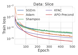
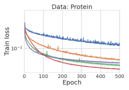
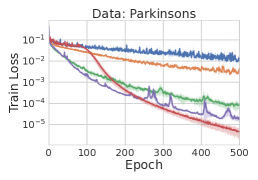
Figure 3: A comparison of SGDm, Adam, KFAC, Shampoo, and APO-Precond on UCI regression tasks. Across all tasks, APO-Precond achieves lower loss with competitive convergence compared to second-order optimizers.

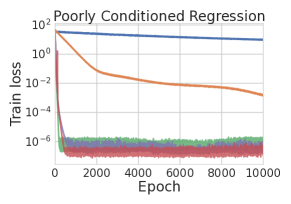
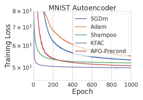
Figure 4: A comparison of various optimizers on optimization tasks known to be difficult for first-order methods. Left: synthetic data for poorly-conditioned regression; Right: deep autoencoder on MNIST.

6.2.2 Image Reconstruction

We trained an 8-layer autoencoder on MNIST (LeCun, 1988); this is known to be a challenging optimization task for first-order optimizers (Hinton & Salakhutdinov, 2006; Martens & Sutskever, 2011; Martens & Grosse, 2015). We followed the experimental set-up from Martens & Grosse (2015), where the encoder and decoder consist of 4 fully-connected layers with sigmoid activation. The decoder structure is symmetric to that of the encoder, and they do not have tied weights. The logistic activation function and the presence of a bottleneck layer make this a challenging optimization problem compared with most current-day architectures. We compare APO-Precond with SGDm, Adam, Shampoo, and KFAC optimizers and show the training losses for each optimizer in Figure 4 (right). APO-Precond converges faster than first-order methods and achieves competitive training loss to other second-order methods (although there remains a performance gap compared with KFAC).

Task	Model	SGDm	Adam	KFAC	APO-Precond
CIFAR-10	LeNet	75.73	73.41	76.63	77.42
CIFAR-10	AlexNet	76.27	76.09	78.33	81.14
CIFAR-10	VGG16	91.82	90.19	92.05	92.13
CIFAR-10	ResNet-18	93.69	93.27	94.60	94.75
CIFAR-10	ResNet-32	94.40	93.30	94.49	94.83
CIFAR-100	AlexNet	43.95	41.82	46.24	52.35
CIFAR-100	VGG16	65.98	60.61	61.84	67.95
CIFAR-100	ResNet-18	76.85	70.87	76.48	76.88
CIFAR-100	ResNet-32	77.47	68.67	75.70	77.41
SVHN	ResNet-18	96.19	95.59	96.08	96.89
IWSLT14	Transformer	31.43	34.60	-	34.62

Table 2: Test accuracy on CIFAR-10 and CIFAR-100, and BLEU score on the IWSLT’14 German-to-English translation dataset for various optimizers.

6.2.3 Image Classification

To investigate whether adapting the preconditioner with APO leads to better generalization, we conducted image classification experiments on CIFAR-10 and CIFAR-100. We trained LeNet (LeCun, 1988), AlexNet (Krizhevsky et al., 2012), VGG-16 (Simonyan & Zisserman, 2014) (w/o batch normalization (Ioffe & Szegedy, 2015)), ResNet-18, and ResNet-32 (He et al., 2016) architectures for 200 epochs with batches of 128 images. For all optimizers, we decayed the learning rate by a factor of 5 at epochs 60, 120, and 160, following common practice from Zagoruyko & Komodakis (2016). The test accuracies for SGDm, Adam, KFAC, and APO-Precond are summarized in Table 2. By adapting the preconditioning matrix with our proximal meta-objective, APO-Precond achieved competitive generalization performance to SGDm. Moreover, for architectures without batch normalization (e.g. LeNet and AlexNet), APO-Precond improved the final test accuracy significantly.

6.2.4 Neural Machine Translation

To verify the effectiveness of APO on various tasks, we applied APO-Precond on the IWSLT’14 German-to-English translation task (Cettolo et al., 2014). We used a Transformer (Vaswani et al., 2017) composed of 6 encoder and decoder layers with a word embedding and hidden vector dimension of 512. We compared APO-Precond with SGDm and AdamW (Loshchilov & Hutter, 2017). For AdamW, we used a warmup-then-decay learning rate schedule widely used in practice, and for SGD and APO-Precond, we kept the learning rate fixed after the warmup. In Table 2, we show the final test BLEU score for SGDm, AdamW, and APO-Precond. While keeping the learning rate fixed, APO-Precond achieved a BLEU score competitive with AdamW.

6.2.5 Low Precision Training

Task	Model	SGDm	KFAC	APO-P
CIFAR-10	LeNet	75.65	74.95	77.25
CIFAR-10	ResNet-18	94.15	92.72	94.79
CIFAR-100	ResNet-18	73.53	73.12	75.47

Table 3: Test accuracy of 16-bit networks on CIFAR-10/100.

Low precision training presents a challenge for second-order optimizers such as KFAC which rely on matrix inverses that may be sensitive to quantization noise. We trained LeNet and ResNet-18 with a 16-bit floating-point arithmetic to examine if APO-Precond is applicable in training the networks in lower precision. We used the same experimental setup from the image classification experiments but stored parameters, activations, and gradients in 16-bit floating-point. We found that KFAC sometimes required a large damping in order to maintain stability, and this prevented it from fully utilizing the curvature information. By contrast, as APO-Precond does not require matrix inversion, it remained stable with the same choice of FSD and WSD weights we used in the full precision experiments. The final test accuracies on ResNet-18 for SGDm, KFAC, and APO-Precond are shown in Table 3. APO-Precond achieved the highest accuracy on both CIFAR-10 and CIFAR-100, whereas KFAC had a $\sim 2\%$ decrease in accuracy. The training curves for ResNet-18 are provided in Appendix C.5.

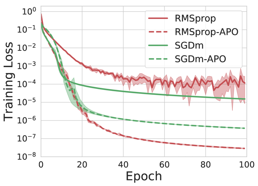
Figure 5: Training loss for a two-layer MLP trained on MNIST, using SGDm and RMSprop (solid lines), and their APO-tuned variants (dashed lines).

6.3 Meta-Learning Learning Rates

MNIST.

First, we compared SGDm and RMSprop to their APO-tuned variants to train an MLP on MNIST. We used a two-layer MLP with 1000 hidden units per layer and ReLU activation, and trained on mini-batches of size 100 for 100 epochs. Figure 5 shows the training loss achieved by each approach; we found that for both base optimizers, APO improved convergence speed and obtained substantially lower loss than the baselines.

CIFAR-10 & CIFAR-100.

For learning rate adaptation on CIFAR-10, we experimented with three network architectures: ResNet32 (He et al., 2016), ResNet34, and WideResNet (WRN-28-10) (Zagoruyko & Komodakis, 2016). For ResNet32, we trained for 400 epochs, and the decayed baseline used a step schedule with $10\times$ decay at epochs 150 and 250, following Lucas et al. (2019). For ResNet34 and WRN-28-10, we trained for 200 epochs, and the decayed baseline used a step schedule with $5\times$ decay at epochs 60, 120, and 160, following Zagoruyko & Komodakis (2016). For CIFAR-100, we used WRN-28-10 with the same schedule as for CIFAR-10. For each of the base optimizers, we compared APO to (1) the optimal fixed learning rate and (2) a manual step learning rate decay schedule. The test accuracies for each base optimizer and their APO-tuned variants are shown in Table 4. In addition, Figure 6 shows the training loss, test accuracy and learning rate adaptation for WRN-28-10 on CIFAR-10, using SGDm as the base optimizer. We found that using APO to tune the global learning rate yields higher test accuracy (or lower training loss) than the best fixed learning rate, and is competitive with the manual decay schedule.

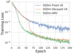
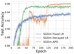
Figure 6: A comparison of the training loss (left), test accuracy (middle), and learning rate schedules (right) of baselines with fixed and decayed learning rates trained on WideResNet 28-10 with CIFAR-10. The training loss plot is shown using hyperparameters chosen based on training loss, while the middle and right plots use hyperparameters chosen based on validation accuracy.

	CIFAR-10 ResNet-32			CIFAR-10 ResNet-34			CIFAR-10 WRN 28-10			CIFAR-100 WRN 28-10
	Fixed	Decay	APO	Fixed	Decay	APO	Fixed	Decay	APO	Fixed	Decay	APO
SGD	90.07	93.30	92.71	93.00	93.54	94.27	93.38	94.86	94.85	76.29	77.92	76.87
SGDm	89.40	93.34	92.75	92.99	95.08	94.47	93.46	95.98	95.50	74.81	81.01	79.33
RMSprop	89.84	91.94	91.28	92.87	93.87	93.97	92.91	93.60	94.22	72.06	76.06	74.17
Adam	90.45	92.26	91.81	93.23	94.12	93.80	92.81	94.04	93.83	72.01	75.53	76.33

Table 4: A comparison of the test accuracies achieved by the optimal fixed learning rate, the manual step decay schedule, and the APO-discovered schedule, using ResNet-32 (He et al., 2016) and WideResNet 28-10 (Zagoruyko & Komodakis, 2016). APO outperforms the optimal fixed learning rate, and is competitive with manual schedule. Note that APO generally achieves test accuracy similar to manual schedules in fewer iterations (shown in App. C).

7 Conclusion

We introduced Amortized Proximal Optimization (APO), a framework for online meta-learning of optimization parameters which approximates the proximal point method by learning a parametric update rule. The update rule is adapted to better minimize a combination of the current-batch loss, function space discrepancy, and weight space discrepancy. As the meta-parameters are updated only once per $K$ steps of optimization, APO incurs minimal computational overhead. We applied the APO framework to two settings: (1) meta-learning the global learning rate for existing base optimizers such as SGD, RMSprop, and Adam and (2) meta-learning structured preconditioning matrices, which provides a new approach to second-order optimization. For preconditioning adaptation problem, we showed that, under certain assumptions, exactly solving the meta-objective recovers classic second-order methods. Compared to other second-order methods such as KFAC, APO eliminates the need to compute matrix inverses, enabling greater efficiency and numerical stability. Adapting update rules to a single meta-objective also opens up the possibility of coming up with even more clever update rules which are better able to exploit the structure of the optimization landscape.

Appendix

This appendix is structured as follows:

• In Section A, we provide an overview of the notation we use throughout the paper.

• In Section B, we provide experiment details.

• In Section C, we provide additional experimental results.

• In Section D, we provide an ablation investigating the difference between evaluating the loss term on the same minibatch used to compute the base optimizer step vs a separate randomly-sampled minibatch. Using a separate random minibatch yields a similar meta-objective to that studied in Wu et al. (2018), which suffers from short-horizon bias.

• In Section E, we provide a derivation of Eq. 4.

• In Section F, we derive classic first- and second-order optimization algorithms (gradient descent, Newton’s method, and natural gradient) starting from the proximal objective for the PPM (Eq. 3).

• In Section G, we provide the proof for Theorem 1, which shows that exactly optimizing the approximate proximal meta-objective with respect to the preconditioner $\mathbf{P}$ can recover various first- and second-order optimization methods.

• In Section H, we list the KFAC assumptions and prove Corollary 2, which shows that under the assumptions of Theorem 1 and the KFAC assumptions, exactly optimizing the approximate proximal meta-objective yields the KFAC update.

• In Section I, we show an ablation over $\lambda_{\text{WSD}}$ and $\lambda_{\text{FSD}}$, and evaluate how well APO performs with different meta-update intervals.

Appendix A Table of Notation

Notation	Description
$\mathcal{D}$	Data-generating distribution
$\mathcal{D}_{\text{train}}$	Finite training dataset
$(\mathbf{x},\mathbf{t})\sim\mathcal{D}$	An input/target pair
$\mathcal{B}$	Mini-batch of data
$N$	Number of training data points, $N=|\mathcal{D}_{\text{train}}|$
${\bm{\theta}}$	Network parameters
$\bm{\phi}$	Optimization parameters (e.g. learning rate or preconditioning matrix)
$\mathbf{P}$	Preconditioning matrix
$\mathbf{G}$	Hessian of the function-space discrepancy
$\mathbf{W}$	Weight matrix of some particular layer of the network
$\mathbf{P}_{\text{S}}$	Structured preconditioner, $\mathbf{P}_{\text{S}}=(\mathbf{A}\otimes\mathbf{B})\text{diag}(\text{vec}(\mathbf{S}))^{2}(\mathbf{A}\otimes\mathbf{B})^{\top}$
$\mathbf{A},\mathbf{B},\mathbf{S}$	Block matrices for EKFAC parameterization
$\lambda$	Weighting of the discrepancy term in the PPM
$\lambda_{\text{FSD}}$	Weighting of the function-space discrepancy term
$\lambda_{\text{WSD}}$	Weighting of the weight-space discrepancy term
$\eta$	Base optimizer learning rate
$\alpha$	Meta optimizer learning rate
$K$	Meta update interval
$p$	Number of optimization hyperparameters
$m$	Number of parameters
$f(\mathbf{x},\bm{\theta})$	Network function with parameters $\bm{\theta}$ applied to input $\mathbf{x}$
$\mathcal{L}(\mathbf{y},\mathbf{t})$	Loss function (e.g. mean-squared error or cross-entropy)
$\mathcal{J}({\bm{\theta}})$	Cost function, $\mathcal{J}({\bm{\theta}})=\frac{1}{N}\sum_{i=1}^{N}\mathcal{L}(f(\mathbf{x}^{(i)},{\bm{\theta}}),\mathbf{t}^{(i)})$
$\mathcal{J}_{\mathcal{B}}({\bm{\theta}})$	Loss on a mini-batch of data, $\mathcal{J}_{\mathcal{B}}({\bm{\theta}})=\frac{1}{|\mathcal{B}|}\sum_{(\mathbf{x},\mathbf{t})\sim\mathcal{B}}\mathcal{L}(f(\mathbf{x},{\bm{\theta}}),\mathbf{t})$
$\mathcal{Q}(\bm{\phi})$	Proximal meta-objective function
$\hat{\mathcal{Q}}(\bm{\phi})$	Approximate proximal meta-objective function
$\rho(\cdot,\cdot)$	Output-space divergence (e.g. KL divergence)
$D(\cdot,\cdot)$	Discrepancy function for the PPM
$D_{\text{F}}(\cdot,\cdot,\cdot)$	Function-space discrepancy function
$D_{\text{W}}(\cdot,\cdot)$	Weight-space discrepancy function
$\text{vec}(\cdot)$	Vectorization function
$\text{diag}(\cdot)$	Diagonalization function
$u({\bm{\theta}},\bm{\phi},\mathcal{B})$	Base optimizer update (e.g. stochastic gradient descent)
${\bm{\theta}}^{\prime}(\bm{\phi})$	Shorthand for $u({\bm{\theta}},\bm{\phi},\mathcal{B})$ where the data $\mathcal{B}$ is implicit
$\otimes$	Kronecker product
$\odot$	Elementwise product

Table 5: A summary of notation used in this paper.

Appendix B Experimental Details

B.1 Computing Environment

All experiments were implemented using the PyTorch (Paszke et al., 2019) and JAX (Bradbury et al., 2018) libraries, and we ran all experiments on NVIDIA P100 GPUs.

B.2 Regression on UCI Collection

We used Slice, Protein, and Parkinson data from the UCI collection. In training, we normalized the input features and targets to have a zero mean and unit variance. We used batch size of 128 and trained the network for 500 epochs without weight decay.

We conducted hyperparameter searches over learning rates for all baseline models, making choices based on the final training loss. With the chosen set of hyperparameters, we repeated the experiments 3 times with different random seeds. For SGDm, we set the momentum to 0.9 and swept over the learning rates {1, 0.3, 0.1, 0.03, 0.01, 0.003, 0.001, 0.0003, 0.0001}. For Adam, we performed a grid search on learning rate of {1e-2, 3e-3, 1e-3, 3e-4, 3e-4, 1e-4}. For Shampoo, we swept over the learning rates {10, 5, 1, 0.3, 0.1, 0.03, 0.01, 0.003, 0.001} as suggested by Gupta et al. (2018). For KFAC, we did a grid search on learning rates of {0.03, 0.01, 0.003, 0.001, 0.0003, 0.0001} and damping values of {3e-2, 1e-2, 3e-3, 1e-3, 3e-4, 1e-4}. For APO-Precond, we set $\lambda_{\text{FSD}}=0$ and grid searched over $\lambda_{\text{WSD}}=\{3,1,0.1,0.01\}$.

B.3 Image Reconstruction

We used the same experimental set-up from Martens & Grosse (2015) for the deep autoencoder experiment. The loss function was defined to be the binary entropy and we further added a regularization term $\frac{\lambda_{\text{WD}}}{2}\|{\bm{\theta}}\|^{2}$ to the loss function, where $\lambda_{\text{WD}}=10^{-5}$. The layer widths for the autoencoder were set to be [784, 1000, 500, 250, 30, 250, 500, 1000, 784] and we used the sigmoid activation function. We trained the network for 1000 epochs with the batch size of 512.

We conducted extensive hyperparameter searches for all baseline models, making choices based on the final training loss. With the chosen set of hyperparameters, we repeated the experiments 3 times with different random seeds. For SGDm, we set the momentum to 0.9 and performed a grid search over the learning rates {1, 0.3, 0.1, 0.03, 0.01, 0.003, 0.001, 0.0003, 0.0001}. For Adam, we swept over learning rate of {3e-2, 1e-2, 3e-3, 1e-3, 3e-4, 3e-4, 1e-4, 3e-5, 1e-5}. For Shampoo, we tried setting learning rates in range of {10, 5, 1, 0.3, 0.1, 0.03, 0.01, 0.003, 0.001}. For KFAC, we did a grid search on learning rates of {0.03, 0.01, 0.003, 0.001, 0.0003, 0.0001, 0.00003, 0.00001} and damping values of {3e-1, 1e-1, 3e-2, 1e-2, 3e-3, 1e-3, 3e-4, 1e-4}. For APO-Precond, we performed a grid search over $\lambda_{\text{FSD}}=\{0.3,0.1\}$ and $\lambda_{\text{WSD}}=\{3,1,0.3,0.1\}$. We set the FSD to measure the KL divergence.

B.4 Image Classification

CIFAR-10 & CIFAR-100.

We used the standard procedure from Zagoruyko & Komodakis (2016) for training convolutional neural networks. The images are zero-padded with 4 pixels on each side and then a random $32\times 32$ crop is extracted from the image, horizontally flipped with the probability of 0.5. We further normalized the inputs with per-channel mean and standard deviations. We performed the extensive search over the hyperparameters for all networks. We held out 5k examples from the CIFAR-10 and CIFAR-100 to form the validation set following Zagoruyko & Komodakis (2016) and selected the hyperparameters with the highest validation accuracy. With the chosen hyperparameters, we re-trained the network with the full training dataset and reported the final test accuracy.

Preconditioning Adaptation.

Across all experiments, we used the batch size of 128 and trained the network for 200 epochs. With the chosen set of hyperparameters, we repeated the experiments 3 times with different random seeds and reported the mean accuracy on the test dataset. For SGDm, we set the momentum to 0.9 and performed a grid search over the learning rates {0.3, 0.1, 0.03, 0.01, 0.003, 0.001, 0.0003, 0.0001}. For Adam, we swept over learning rate of {3e-2, 1e-2, 3e-3, 1e-3, 3e-4, 3e-4, 1e-4}. For KFAC, we did a grid search on learning rates of {0.03, 0.01, 0.003, 0.001, 0.0003, 0.0001, 0.00003, 0.00001} and damping values of {3e-2, 1e-2, 3e-3, 1e-3, 3e-4, 1e-4}. For APO-Precond, we performed a grid search over $\lambda_{\text{FSD}}=\{0.3,0.1\}$ and $\lambda_{\text{WSD}}=\{3,1,0.3,0.1\}$ for architectures without batch normalization. As batch normalization makes the parameters scale-invariant (Arora et al., 2018), we imposed a higher regularization in the function space and lower regularization in the weight space, searching over $\lambda_{\text{FSD}}=\{3,1\}$ and $\lambda_{\text{WSD}}=\{0.3,0.1,0.03,0.01\}$. We set the FSD term to measure the KL divergence. We also searched over the weight decay in range of {5e-4, 1e-4, 5e-5} for all optimizers.

Learning Rate Adaptation.

For ResNet32, we trained for 400 epochs, and used a manual schedule that decays the learning rate by a factor of 10 at epochs 150 and 250, following Lucas et al. (2019). For ResNet34 and WideResNet 28-10, we trained for 200 epochs, with a manual schedule that decays the learning rate by a factor of 5 at epochs 60, 120, and 160, following Zagoruyko & Komodakis (2016).

For the baseline optimizers, we performed grid searches over the fixed learning rate or initial learning rate for a fixed step schedule, as well as the weight decay. For all base optimizers and APO-tuned variants, we searched over weight decay values in $\{0.01,0.003,0.001,0.0003,0.0001,0.0\}$. For SGD and SGDm, we searched over learning rates in $\{1.0,0.3,0.1,0.03,0.01,0.003,0.001,0.0003,0.0001\}$. For RMSprop and Adam, we searched over learning rates in $\{0.1,0.03,0.01,0.003,0.001,0.0003,0.0001,0.00003,0.00001\}$. For each of the APO-tuned variants (e.g. SGDm-APO), we kept $\lambda_{\text{WSD}}=0$ and searched over $\lambda_{\text{FSD}}\in\{0.3,0.1,0.03,0.01,0.003,0.001,0.0003,0.0001\}$.

B.5 Neural Machine Translation

We trained a Transformer (Vaswani et al., 2017) composed of 6 encoder and decoder layers, with a word embedding and hidden vector dimension of 512. The architecture has feed-forward size of 1024, 4 attention heads, dropout value 0.3, and weight decay value 0.0001. For APO-Precond, following the practice from Zhang et al. (2019a), we used a diagonal block matrix in the structured preconditioner of the embedding weight matrix to reduce memory overhead. We used the Fairseq toolkit (Ott et al., 2019) to conduct all experiments.

For SGDm, we grid searched over the learning rates in {10, 3, 1, 0.3, 0.1, 0.03, 0.01, 0.003, 0.001} and tried both the fixed learning rate and inverse sqrt learning rate schedules. For AdamW, we set $\beta_{1}=0.9$, $\beta_{2}=0.98$, and $\epsilon=10^{-1}$ and searched over the learning rates in range {0.05, 0.001, 0.0005, 0.0001}. AdamW also used the inverse sqrt learning rate schedule with 4000 warmup steps. For APO-Precond, we searched over $\lambda_{\text{FSD}}=\{0.3,0.1\}$ and $\lambda_{\text{WSD}}=\{3,1,0.3,0.1\}$ and let FSD term to measure the KL divergence. As we found a fixed learning rate schedule to work best for SGDm, we also used a fixed learning rate schedule for APO-Precond. We selected the hyperparameters based on the BLEU score on the validation set and reported on the final test BLEU score on the checkpoint, which achieved the highest validation BLEU score.

Appendix C Additional Results

C.1 Rosenbrock Function

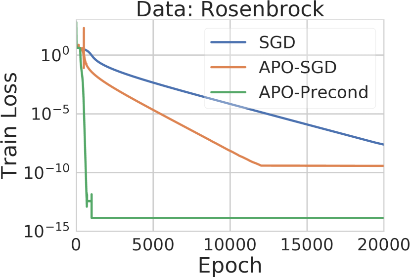
Figure 7: Training loss on the Rosenbrock function. Both the learning rate schedules and the preconditioner adapted by APO outperform the optimal fixed learning rate for SGD.

We validated APO on the two-dimensional Rosenbrock function defined as:

$$f(x,y)=(1-x)^{2}+100(y-x^{2})^{2}$$

with initialization $(x,y)=(1,-1.5)$. In Figure 7, we used APO to tune the learning rate for SGD, as well as the full preconditioning matrix. Both APO-tuned methods outperformed vanilla SGD with the optimal fixed learning rate (chosen through a careful grid search). Because Rosenbrock has ill-conditioned curvature, second-order optimization with APO-Precond dramatically speeds up the convergence and achieves a lower loss.

C.2 SVHN

We also evaluated APO on the Google Street View House Numbers dataset (SVHN) (Netzer et al., 2011), using a WideResNet 16-8. We followed the experimental setup of Zagoruyko & Komodakis (2016), and used the same decay schedule for the baseline, which decays the learning rate by $10\times$ at epochs 80 and 120. The optimal fixed learning rate achieves test accuracy fluctuating around 97.20%, while the manual schedule achieves 98.17%. APO rapidly converges to test accuracy 97.96%, outperforming the baseline while being slightly worse than the manual schedule (Figure 8).

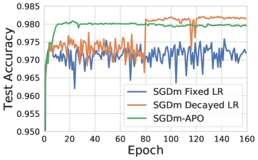
Figure 8: Test Accuracy on SVHN using SGDm with fixed learning rate, decayed learning rate schedule, and APO-tuned learning rate.

C.3 CIFAR-10

APO Preconditioning Adaptation.

We show the plots for for experiments listed in Table 2 in Figure 9 and Figure 10.

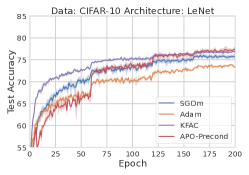
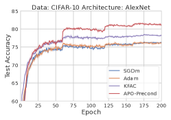
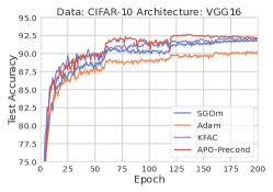
Figure 9: LeNet, AlexNet, and VGG16 on CIFAR-10, using SGDm, Adam, KFAC, and APO-Precond.

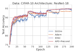
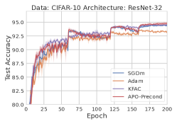
Figure 10: ResNet-18 and ResNet-32 on CIFAR-10, using SGDm, Adam, KFAC, and APO-Precond.

APO Learning Rate Schedules.

We show the plots for each base-optimizer and network architecture as below. We find that APO achieves better performance than the best fixed LR, and is comparable to the manual schedule. The learning rate schedules discovered by APO are nontrivial: most exhibit a large increase in the learning rate at the start of training to make rapid progress, followed by a gradual decrease in the learning rate to fine-tune the solution as optimization approaches a local optimum. The APO learning rate schedules often span two orders of magnitude, similarly to manual decay schedules.

	CIFAR-10 (ResNet34)
	Fixed	Decayed	APO
SGD	93.00 $\pm$ 0.35	93.54 $\pm$ 0.01	94.27 $\pm$ 0.02
SGDm	92.99 $\pm$ 0.14	95.08 $\pm$ 0.24	94.47 $\pm$ 0.24
RMSprop	92.87 $\pm$ 0.32	93.97 $\pm$ 0.11	93.97 $\pm$ 0.07
Adam	93.23 $\pm$ 0.15	94.12 $\pm$ 0.10	93.80 $\pm$ 0.14

Table 6: Test accuracy on CIFAR-10 using ResNet34. APO consistently outperforms the best fixed learning rate for each optimizer, and is on par with carefully-tuned manual schedules. Each reported result is the mean of 4 random restarts, and we report $\pm$ the standard deviation.

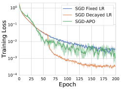
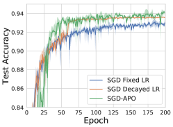
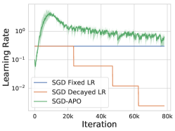
Figure 11: ResNet34 on CIFAR-10, using SGD. The shaded regions show the min/max values over 4 random restarts.

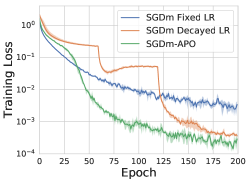
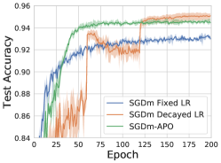
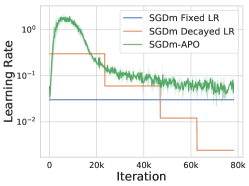
Figure 12: ResNet34 on CIFAR-10, using SGDm. The shaded regions show the min/max values over 4 random restarts.

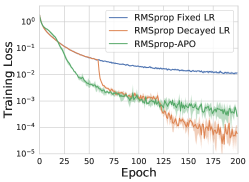
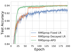
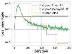
Figure 13: ResNet34 on CIFAR-10, using RMSprop. The shaded regions show the min/max values over 4 random restarts.

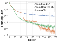
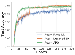
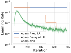
Figure 14: ResNet34 on CIFAR-10, using Adam. The shaded regions show the min/max values over 4 random restarts.

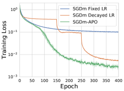
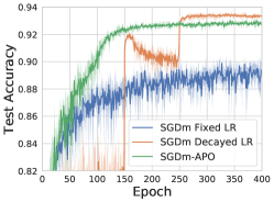
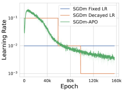
Figure 15: ResNet32 on CIFAR-10, using SGDm. The shaded regions show the min/max values over 4 random restarts.

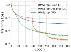
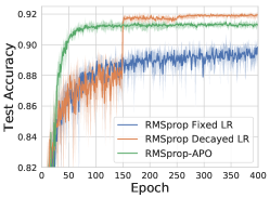
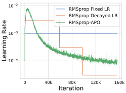
Figure 16: ResNet32 on CIFAR-10, using RMSprop. The shaded regions show the min/max values over 4 random restarts.

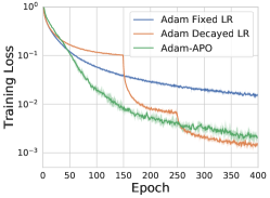
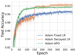
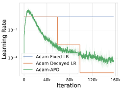
Figure 17: ResNet32 on CIFAR-10, using Adam. The shaded regions show the min/max values over 4 random restarts.

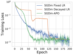
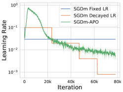
Figure 18: WideResNet 28-10 on CIFAR-10, using SGDm. The shaded regions show the min/max values over 4 random restarts.

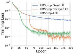
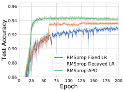
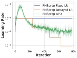
Figure 19: WideResNet 28-10 on CIFAR-10, using RMSprop. The shaded regions show the min/max values over 4 random restarts.

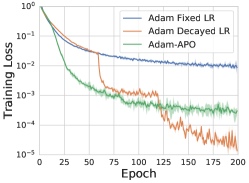
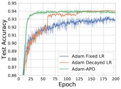
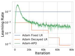
Figure 20: WideResNet 28-10 on CIFAR-10, using Adam. The shaded regions show the min/max values over 4 random restarts.

C.4 CIFAR-100

APO Learning Rate Schedules.

We show training curve plots for different base-optimizers below. We find that APO usually achieves better performance than fixed LR, and is comparable with the manual schedule.

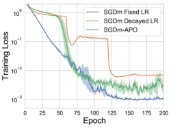
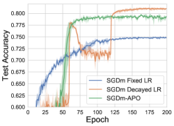
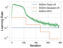
Figure 21: WideResNet on CIFAR-100, using SGDm. The shaded regions show the min/max values over 4 random restarts.

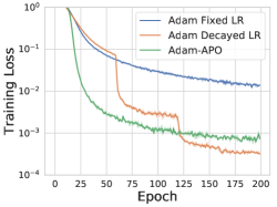
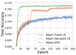
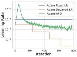
Figure 22: WideResNet on CIFAR-100, using Adam. The shaded regions show the min/max values over 4 random restarts.

C.5 16-bit Neural Network Training

We show the training curve plots for training 16-bit ResNet-18 on CIFAR-10 and CIFAR-100 in Figure 23 .

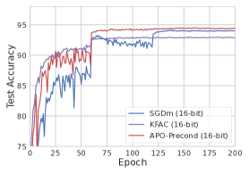
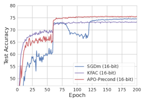
Figure 23: Test accuracy curves for 16-bit neural networks: ResNet-18 on CIFAR-10 (left) and CIFAR-100 (right).

Appendix D Importance of Using the Same Minibatch

In this section, we empirically verify the importance of computing the first term of the meta-objective on the same mini-batch that is used to compute the gradient of the base optimizer. Recall that our meta-objective is:

$$\mathcal{Q}(\bm{\phi})=\mathcal{J}_{{\color[rgb]{0,0.6,0}\mathcal{B}}}(u(\bm{\theta},\bm{\phi},{\color[rgb]{0,0.6,0}\mathcal{B}}))+\lambda_{\text{FSD}}\mathbb{E}_{({\color[rgb]{0,0,1}\tilde{\mathbf{x}}},\cdot)\sim\mathcal{D}}[D_{\text{F}}(u(\bm{\theta},\bm{\phi},{\color[rgb]{0,0.6,0}\mathcal{B}}),\bm{\theta},{\color[rgb]{0,0,1}\tilde{\mathbf{x}}})]+\frac{\lambda_{\text{WSD}}}{2}||u(\bm{\theta},\bm{\phi},{\color[rgb]{0,0.6,0}\mathcal{B}})-\bm{\theta}||_{2}^{2}$$ (12)

Note that the loss term is computed using the same mini-batch ${\color[rgb]{0,0.6,0}\mathcal{B}}$ used for the update $u(\bm{\theta},\bm{\phi},{\color[rgb]{0,0.6,0}\mathcal{B}})$. An alternative is to evaluate the loss term on a randomly-sampled mini-batch ${\color[rgb]{0.8,0.0,0}\mathcal{B}^{\prime}}\sim\mathcal{D}$, yielding:

$$\mathcal{Q}(\bm{\phi})=\mathcal{J}_{{\color[rgb]{0.8,0.0,0}\mathcal{B}^{\prime}}}(u(\bm{\theta},\bm{\phi},{\color[rgb]{0,0.6,0}\mathcal{B}}))+\lambda_{\text{FSD}}\mathbb{E}_{({\color[rgb]{0,0,1}\tilde{\mathbf{x}}},\cdot)\sim\mathcal{D}}[D_{\text{F}}(u(\bm{\theta},\bm{\phi},{\color[rgb]{0,0.6,0}\mathcal{B}}),\bm{\theta},{\color[rgb]{0,0,1}\tilde{\mathbf{x}}})]+\frac{\lambda_{\text{WSD}}}{2}||u(\bm{\theta},\bm{\phi},{\color[rgb]{0,0.6,0}\mathcal{B}})-\bm{\theta}||_{2}^{2}$$ (13)

If we set $\lambda_{\text{FSD}}=\lambda_{\text{WSD}}=0$, then Eq. 13 becomes the meta-objective analyzed by Wu et al. (2018), which was used to illustrate the short-horizon bias issue in stochastic meta-optimization.

Figure 24 shows the result of using Eq. 12 vs. Eq. 13 for meta-optimizing the learning rate of a ResNet32 model on CIFAR-10. We observe that when using a random minibatch ${\color[rgb]{0.8,0.0,0}\mathcal{B}^{\prime}}$ to compute the loss term, the learning rate decays rapidly, preventing long-term progress; in contrast, using the same minibatch ${\color[rgb]{0,0.6,0}\mathcal{B}}$ for the loss term yields a resonable LR schedule which does not suffer from the short-horizon bias issue empirically.

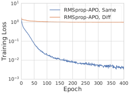
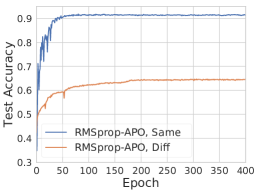
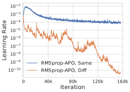
Figure 24: Left: Training loss compared between 1) using the same mini-batch for the first term and 2) using a different mini-batch for the first term. Right: Comparison of learning rates for the two conditions.

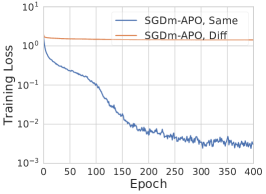
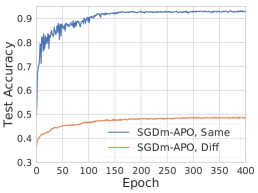
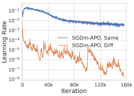
Figure 25: Left: Training loss compared between 1) using the same mini-batch for the first term and 2) using a different mini-batch for the first term. Right: Comparison of learning rates for the two conditions.

Same Mini-Batch for the FSD Term.

Another alternative to the meta-objective is to compute the FSD term using the same mini-batch used to compute the loss term, as shown in Eq. 14.

$$\mathcal{Q}(\bm{\phi})=\mathcal{J}_{{\color[rgb]{0,0.6,0}\mathcal{B}}}(u(\bm{\theta},\bm{\phi},{\color[rgb]{0,0.6,0}\mathcal{B}}))+\frac{\lambda_{\text{FSD}}}{|{\color[rgb]{0,0.6,0}\mathcal{B}}|}\sum_{({\color[rgb]{0,0.6,0}\tilde{\mathbf{x}}},\cdot)\in{\color[rgb]{0,0.6,0}\mathcal{B}}}D_{\text{F}}(u(\bm{\theta},\bm{\phi},{\color[rgb]{0,0.6,0}\mathcal{B}}),\bm{\theta},{\color[rgb]{0,0.6,0}\tilde{\mathbf{x}}})+\frac{\lambda_{\text{WSD}}}{2}||u(\bm{\theta},\bm{\phi},{\color[rgb]{0,0.6,0}\mathcal{B}})-\bm{\theta}||_{2}^{2}$$ (14)

Recall that $D_{\text{F}}(u(\bm{\theta},\bm{\phi},{\color[rgb]{0,0.6,0}\mathcal{B}}),\bm{\theta},{\color[rgb]{0,0.6,0}\tilde{\mathbf{x}}})=\rho(f({\color[rgb]{0,0.6,0}\tilde{\mathbf{x}}},u(\bm{\theta},\bm{\phi},{\color[rgb]{0,0.6,0}\mathcal{B}})),f({\color[rgb]{0,0.6,0}\tilde{\mathbf{x}}},\bm{\theta}))$. The function evaluation $f({\color[rgb]{0,0.6,0}\tilde{\mathbf{x}}},u(\bm{\theta},\bm{\phi},{\color[rgb]{0,0.6,0}\mathcal{B}}))$ must be performed to compute the loss term; thus, using the same minibatch ${\color[rgb]{0,0.6,0}\mathcal{B}}$ for the FSD term can allow us to reduce computation by re-using this function output in both the loss and FSD computations. However, with the interpretation of the FSD term in Eq. 14 as a Monte Carlo estimate of the expectation $\mathbb{E}_{\tilde{\mathbf{x}}\sim\mathcal{D}}[D_{\text{F}}(u(\bm{\theta},\bm{\phi},\mathcal{B}),\bm{\theta},\tilde{\mathbf{x}})]$, using the same mini-batch for the loss and dissimilarity would yield a biased estimate. The effect of using a different vs the same mini-batch to compute the FSD term is shown in Figure 26.

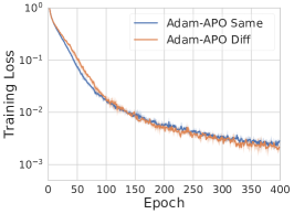
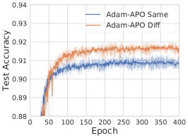
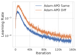
Figure 26: Left: Training loss compared between 1) using the same mini-batch for the second term as for the first term of the meta-objective and 2) using a different mini-batch for the second term. Right: Comparison of learning rates for the two conditions.

Appendix E Approximate Closed-Form Solution for the PPM

In Section 3.1, we introduced a general update rule for the stochastic PPM, which is defined as follows:

$${\bm{\theta}}^{(t+1)} \leftarrow\operatorname*{arg\,min}_{\mathbf{u}\in\mathbb{R}^{m}}\mathcal{J}_{\mathcal{B}}(\mathbf{u})+\lambda_{\text{FSD}}\mathbb{E}_{\tilde{\mathbf{x}}\sim\mathcal{D}}[D_{\text{F}}(\mathbf{u},{\bm{\theta}}^{(t)},\mathbf{x})]+\lambda_{\text{WSD}}D_{\text{W}}(\mathbf{u},{\bm{\theta}}^{(t)}).$$ (15)

We first take the infinitesimal limit by letting $\lambda_{\text{FSD}}\to\infty$. Then, the optimal update $\mathbf{u}^{\star}$ will stay close to the current parameters ${\bm{\theta}}^{(t)}$ and we can approximate the loss function with the first-order Taylor approximation. Moreover, since the FSD term $\mathbb{E}_{\tilde{\mathbf{x}}\sim\mathcal{D}}[D_{\text{F}}(\mathbf{u},{\bm{\theta}}^{(t)},\mathbf{x})]$ is minimized when $\mathbf{u}={\bm{\theta}}^{(t)}$, we have $\nabla_{\mathbf{u}}\mathbb{E}_{\tilde{\mathbf{x}}\sim\mathcal{D}}[D_{\text{F}}(\mathbf{u},{\bm{\theta}}^{(t)},\mathbf{x})]|_{\mathbf{u}={\bm{\theta}}^{(t)}}=\mathbf{0}$. Hence, the second-order Taylor expansion of the FSD term would be:

$$\mathbb{E}_{\tilde{\mathbf{x}}\sim\mathcal{D}}[D_{\text{F}}(f(\tilde{\mathbf{x}},\mathbf{u}),f(\tilde{\mathbf{x}},\bm{\theta}^{(t)}))]\approx\frac{1}{2}(\mathbf{u}-{\bm{\theta}}^{(t)})^{\top}\mathbf{G}(\mathbf{u}-{\bm{\theta}}^{(t)}),$$ (16)

where $\mathbf{G}=\nabla^{2}_{\mathbf{u}}\mathbb{E}_{\tilde{\mathbf{x}}\sim\mathcal{D}}[D_{\text{F}}(\mathbf{u},{\bm{\theta}}^{(t)},\mathbf{x})]|_{\mathbf{u}={\bm{\theta}}^{(t)}}$ is the local Hessian of the FSD term. We further let the weight space discrepancy function to be the squared Euclidean distance $D_{\text{W}}(\mathbf{u},{\bm{\theta}}^{(t)})=\nicefrac{{1}}{{2}}\|\mathbf{u}-{\bm{\theta}}^{(t)}\|^{2}_{2}$. Combining these insights, we approximate Eqn. 15 by linearzing the loss and taking a quadratic approximation to the FSD term:

$${\bm{\theta}}^{(t+1)}\approx\operatorname*{arg\,min}_{\mathbf{u}\in\mathbb{R}^{m}}\left[\nabla_{{\bm{\theta}}}\mathcal{J}_{\mathcal{B}}({\bm{\theta}}^{(t)})^{\top}(\mathbf{u}-{\bm{\theta}}^{(t)})+\frac{\lambda_{\text{FSD}}}{2}(\mathbf{u}-{\bm{\theta}}^{(t)})^{\top}\mathbf{G}(\mathbf{u}-{\bm{\theta}}^{(t)})+\frac{\lambda_{\text{WSD}}}{2}\|\mathbf{u}-{\bm{\theta}}^{(t)}\|^{2}\right].$$ (17)

Taking the gradient with respect to $\mathbf{u}$ and setting it equal to $\mathbf{0}$, we have:

$$\nabla_{{\bm{\theta}}}\mathcal{J}_{\mathcal{B}}({\bm{\theta}}^{(t)})+\lambda_{\text{FSD}}\mathbf{G}\mathbf{u}-\lambda_{\text{FSD}}\mathbf{G}{\bm{\theta}}^{(t)}+\lambda_{\text{WSD}}\mathbf{u}-\lambda_{\text{WSD}}{\bm{\theta}}^{(t)}=\mathbf{0}.$$ (18)

Rearranging the terms, we arrive at the approximate closed-form solution:

$$\mathbf{u}^{\star}\approx{\bm{\theta}}^{(t)}-(\lambda_{\text{FSD}}\mathbf{G}+\lambda_{\text{WSD}}\mathbf{I})^{-1}\nabla_{{\bm{\theta}}}\mathcal{J}_{\mathcal{B}}({\bm{\theta}}^{(t)}).$$ (19)

Appendix F Optimization Algorithms Derived from the Proximal Objective

In this section, we show how several classical optimization algorithms can be derived from the proximal objective introduced in Section 3.2. Given a mini-batch $\mathcal{B}$, recall that we consider the following proximal objective for optimizing the model parameters $\bm{\theta}$:

$$\bm{\theta}^{(t+1)} =\operatorname*{arg\,min}_{\bm{\theta}\in\mathbb{R}^{m}}\left\{\mathcal{J}_{\mathcal{B}}(\bm{\theta})+\lambda_{\text{FSD}}\mathbb{E}_{\tilde{\mathbf{x}}}[D_{\text{F}}(\bm{\theta},{\bm{\theta}}^{(t)},\tilde{\mathbf{x}})]+\frac{\lambda_{\text{WSD}}}{2}||\bm{\theta}-\bm{\theta}^{(t)}||_{2}^{2}\right\}.$$ (20)

Method	Loss Term Approx. $\mathcal{J}_{\mathcal{B}}(\mathbf{u})$	FSD Term Approx. $D_{\text{F}}(\mathbf{u},{\bm{\theta}},\mathbf{x})$	FSD Term Choice of $D_{\text{F}}$	WSD Term $\frac{1}{2}||\mathbf{u}-\bm{\theta}||^{2}$
Gradient Descent	$1^{\text{st}}$-order	-	-	✓
Newton’s Method	$2^{\text{nd}}$-order	-	-	✗
Damped Newton’s Method	$2^{\text{nd}}$-order	-	-	✓
Natural Gradient	$1^{\text{st}}$-order	$2^{\text{nd}}$-order	KL	✗
Damped Natural Gradient	$1^{\text{st}}$-order	$2^{\text{nd}}$-order	KL	✓
Generalized Gauss-Newton	$1^{\text{st}}$-order	$2^{\text{nd}}$-order	Bregman	✗
Damped Generalized Gauss-Newton	$1^{\text{st}}$-order	$2^{\text{nd}}$-order	Bregman	✓
Direct Proximal Optimization	Exact	Exact	Any	✓

F.1 Gradient Descent

To derive vanilla gradient descent, we take the first-order Taylor series approximation to the loss term $\mathcal{J}_{\mathcal{B}}(\bm{\theta})$ about $\bm{\theta}^{(t)}$, and set $\lambda_{\text{FSD}}=0$. We need to have $\lambda_{\text{WSD}}>0$ to ensure that we do not take an infinitely large step. Thus, each step of gradient descent minimizes an approximation to the proximal objective which we denote by $P^{\text{GD}}_{\bm{\theta}^{(t)}}(\bm{\theta})$:

$$\bm{\theta}^{(t+1)} =\operatorname*{arg\,min}_{\bm{\theta}}P^{\text{GD}}_{\bm{\theta}^{(t)}}(\bm{\theta}),$$ (21)

where:

$$P^{\text{GD}}_{\bm{\theta}^{(t)}}(\bm{\theta})=\mathcal{J}_{\mathcal{B}}(\bm{\theta}^{(t)})+\nabla\mathcal{J}_{\mathcal{B}}(\bm{\theta}^{(t)})^{\top}(\bm{\theta}-\bm{\theta}^{(t)})+\frac{\lambda_{\text{WSD}}}{2}||\bm{\theta}-\bm{\theta}^{(t)}||_{2}^{2}.$$ (22)

Now, we set the gradient $\nabla_{\bm{\theta}}P^{\text{GD}}_{\bm{\theta}^{(t)}}(\bm{\theta})=0$ and solve for $\bm{\theta}$:

$$\nabla_{\bm{\theta}}\left(\nabla\mathcal{J}_{\mathcal{B}}(\bm{\theta}^{(t)})^{\top}(\bm{\theta}-\bm{\theta}^{(t)})+\frac{\lambda_{\text{WSD}}}{2}||\bm{\theta}-\bm{\theta}^{(t)}||_{2}^{2}\right) =0$$ (23)

$$\nabla\mathcal{J}_{\mathcal{B}}(\bm{\theta}^{(t)})+\lambda_{\text{WSD}}(\bm{\theta}-\bm{\theta}^{(t)}) =0$$ (24)

$$\bm{\theta} =\bm{\theta}^{(t)}-\frac{1}{\lambda_{\text{WSD}}}\nabla\mathcal{J}_{\mathcal{B}}(\bm{\theta}^{(t)})$$ (25)

F.2 Newton’s Method

To derive Newton’s method, we take the second-order Taylor series approximation to the loss term $\mathcal{J}_{\mathcal{B}}(\bm{\theta})$ about $\bm{\theta}^{(t)}$, and set $\lambda_{\text{FSD}}=0$. Below we derive the general form for the damped Newton update, which incorporates the WSD term; setting $\lambda_{\text{WSD}}=0$ leads to the undamped Newton update as a special case. Each step of Newton’s method minimizes an approximation to the proximal objective which we denote by $P^{\text{Newton}}_{\bm{\theta}^{(t)}}(\bm{\theta})$:

$$\bm{\theta}^{(t+1)} =\operatorname*{arg\,min}_{\bm{\theta}}P^{\text{Newton}}_{\bm{\theta}^{(t)}}(\bm{\theta}),$$ (26)

where:

$$P^{\text{Newton}}_{\bm{\theta}^{(t)}}(\bm{\theta})=\mathcal{J}_{\mathcal{B}}(\bm{\theta}^{(t)})+\nabla\mathcal{J}_{\mathcal{B}}(\bm{\theta}^{(t)})^{\top}(\bm{\theta}-\bm{\theta}^{(t)})+\frac{1}{2}(\bm{\theta}-\bm{\theta}^{(t)})^{\top}\mathbf{H}(\bm{\theta}-\bm{\theta}^{(t)})+\frac{\lambda_{\text{WSD}}}{2}||\bm{\theta}-\bm{\theta}^{(t)}||_{2}^{2}.$$ (27)

In Eq. 27, $\mathbf{H}=\nabla_{\bm{\theta}}^{2}\mathcal{J}_{\mathcal{B}}(\bm{\theta})$. Now, we set the gradient $\nabla_{\bm{\theta}}P^{\text{Newton}}_{\bm{\theta}^{(t)}}(\bm{\theta})=0$ and solve for $\bm{\theta}$:

$$\nabla_{\bm{\theta}}P^{\text{Newton}}_{\bm{\theta}^{(t)}}(\bm{\theta}) =0$$ (28)

$$\nabla\mathcal{J}_{\mathcal{B}}(\bm{\theta}^{(t)})+\mathbf{H}\bm{\theta}-\mathbf{H}\bm{\theta}^{(t)}+\lambda_{\text{WSD}}\bm{\theta}-\lambda_{\text{WSD}}\bm{\theta}^{(t)} =0$$ (29)

$$(\mathbf{H}+\lambda_{\text{WSD}}\mathbf{I})(\bm{\theta}-\bm{\theta}^{(t)}) =-\nabla\mathcal{J}_{\mathcal{B}}(\bm{\theta}^{(t)})$$ (30)

$$\bm{\theta} =\bm{\theta}^{(t)}-(\mathbf{H}+\lambda_{\text{WSD}}\mathbf{I})^{-1}\nabla\mathcal{J}_{\mathcal{B}}(\bm{\theta}^{(t)})$$ (31)

F.3 Generalized Gauss-Newton Method

Next, we consider taking the first-order Taylor series approximation to the loss term, and an arbitrary function-space discrepancy $D_{\text{F}}$ approximated by its second-order Taylor series expansion. We will use the notation $\mathbf{z}=f(\mathbf{x},\bm{\theta})$ to denote the outputs of a neural network with parameters $\bm{\theta}$ on inputs $\mathbf{x}$. We have the following proximal objective:

$$P_{\bm{\theta}^{(t)}}(\bm{\theta})=\mathcal{J}_{\mathcal{B}}(\bm{\theta}^{(t)})+\nabla\mathcal{J}_{\mathcal{B}}(\bm{\theta}^{(t)})^{\top}(\bm{\theta}-\bm{\theta}^{(t)})+\lambda_{\text{FSD}}\mathbb{E}_{\tilde{\mathbf{x}}}[D_{\text{F}}(\bm{\theta},\bm{\theta}^{(t)},\tilde{\mathbf{x}}))]+\frac{\lambda_{\text{WSD}}}{2}||\bm{\theta}-\bm{\theta}^{(t)}||_{2}^{2}$$ (32)

Taking the second-order approximation to $D_{\text{F}}$ (with respect to $\bm{\theta}$), we have:

$$D_{\text{F}}(\bm{\theta},\bm{\theta}^{(t)})\approx\underbrace{D_{\text{F}}(\bm{\theta}^{(t)},\bm{\theta}^{(t)})}_{=0}+\underbrace{\nabla_{\bm{\theta}}D_{\text{F}}(\bm{\theta},\bm{\theta}^{(t)})|_{\bm{\theta}=\bm{\theta}^{(t)}}^{\top}(\bm{\theta}-\bm{\theta}^{(t)})}_{=0}+\frac{1}{2}(\bm{\theta}-\bm{\theta}^{(t)})^{\top}\nabla_{\bm{\theta}}^{2}D_{\text{F}}(\bm{\theta},\bm{\theta}^{(t)})|_{\bm{\theta}=\bm{\theta}^{(t)}}(\bm{\theta}-\bm{\theta}^{(t)}).$$ (33)

Using the chain rule, we can derive $\nabla_{\bm{\theta}}^{2}D_{\text{F}}(\bm{\theta},\bm{\theta}^{(t)})|_{\bm{\theta}=\bm{\theta}^{(t)}}$ as follows:

$$\nabla_{\bm{\theta}}^{2}D_{\text{F}}(\bm{\theta},\bm{\theta}^{(t)})|_{\bm{\theta}=\bm{\theta}^{(t)}}=\underbrace{\left(\frac{\partial\mathbf{z}}{\partial\bm{\theta}}\right)^{\top}}_{\mathbf{J}_{\mathbf{z}\bm{\theta}}^{\top}}\underbrace{\left(\frac{\partial^{2}\rho}{\partial\mathbf{z}^{2}}\right)}_{\mathbf{H}_{\rho}}\underbrace{\left(\frac{\partial\mathbf{z}}{\partial\bm{\theta}}\right)}_{\mathbf{J}_{\mathbf{z}\bm{\theta}}}=\mathbf{J}_{\mathbf{z}\bm{\theta}}^{\top}\nabla_{\mathbf{z}}^{2}\rho(\mathbf{z},\mathbf{z}^{(t)})\mathbf{J}_{\mathbf{z}\bm{\theta}}=\mathbf{J}_{\mathbf{z}\bm{\theta}}^{\top}\mathbf{H}_{\rho}\mathbf{J}_{\mathbf{z}\bm{\theta}}$$ (34)

Letting $\mathbf{G}$ denote the expectation of the Hessian of the FSD function, $\mathbf{G}=\mathbb{E}_{\tilde{\mathbf{x}}\sim\mathcal{D}}[\nabla_{\bm{\theta}}^{2}D_{\text{F}}(\bm{\theta},\bm{\theta}^{(t)},\tilde{\mathbf{x}})]$, we have:

$$P_{\bm{\theta}^{(t)}}(\bm{\theta})=\mathcal{J}_{\mathcal{B}}(\bm{\theta}^{(t)})+\nabla\mathcal{J}_{\mathcal{B}}(\bm{\theta}^{(t)})^{\top}(\bm{\theta}-\bm{\theta}^{(t)})+\frac{\lambda_{\text{FSD}}}{2}(\bm{\theta}-\bm{\theta}^{(t)})^{\top}\mathbf{G}(\bm{\theta}-\bm{\theta}^{(t)})+\frac{\lambda_{\text{WSD}}}{2}||\bm{\theta}-\bm{\theta}^{(t)}||_{2}^{2}$$ (35)

If we set the gradient $\nabla_{\bm{\theta}}P_{\bm{\theta}^{(t)}}(\bm{\theta})=0$ and solve for $\bm{\theta}$, we obtain:

$$\bm{\theta}=\bm{\theta}^{(t)}-(\lambda_{\text{FSD}}\mathbf{G}+\lambda_{\text{WSD}}\mathbf{I})^{-1}\nabla\mathcal{J}_{\mathcal{B}}(\bm{\theta}^{(t)})$$ (36)

Appendix G Optimizing the 1-Step Meta-Objective Recovers Classic Methods

In this section, we show that when we approximate the loss term and FSD term of our meta-objective $\mathcal{Q}(\bm{\phi})$ and solve for the analytic $\operatorname*{arg\,min}_{\bm{\phi}}\mathcal{Q}(\bm{\phi})$, we recover the preconditioners corresponding to classic first- and second-order algorithms, including gradient descent, Gauss-Newton, Generalized Gauss-Newton, and natural gradient. The preconditioners used by each of these methods are shown in Table 1. These results parallel those for directly optimizing the parameters $\bm{\theta}$ using the proximal objective, but optimizing for the meta-parameters $\bm{\phi}=\mathbf{P}$.

Throughout this exposition, we use the notation:

$$u(\bm{\theta},\bm{\phi},\mathcal{B})=u(\bm{\theta},\mathbf{P},\mathcal{B})=\bm{\theta}-\mathbf{P}\nabla_{\bm{\theta}}\mathcal{J}_{\mathcal{B}}(\bm{\theta})=\bm{\theta}-\mathbf{P}\mathbf{g}$$ (37)

where $\mathbf{g}=\nabla_{\bm{\theta}}\mathcal{J}_{\mathcal{B}}(\bm{\theta})$. Note that $\mathbf{g}$ implicitly depends on the data $\mathcal{B}$; we use this shorthand to simplify the exposition.

Theorem.

Consider an approximation $\hat{\mathcal{Q}}(\mathbf{P})$ to the meta-objective (Eq. 8) where the loss term is linearized around the current weights $\bm{\theta}$ and the FSD term is replaced by its second-order approximation around $\bm{\theta}$:

$$\hat{\mathcal{Q}}(\mathbf{P})= \mathbb{E}_{\mathcal{B}\sim\mathcal{D}}\Big{[}\nabla_{\bm{\theta}}\mathcal{J}_{\mathcal{B}}(\bm{\theta})^{\top}(u(\bm{\theta},\mathbf{P},\mathcal{B})-\bm{\theta})$$

$$\qquad\quad+\lambda_{\text{FSD}}(u(\bm{\theta},\mathbf{P},\mathcal{B})-\bm{\theta})^{\top}\mathbf{G}(u(\bm{\theta},\mathbf{P},\mathcal{B})-\bm{\theta})+\frac{\lambda_{\text{WSD}}}{2}\|u(\bm{\theta},\mathbf{P},\mathcal{B})-{\bm{\theta}}\|^{2}\Big{]}.$$ (38)

Denote the gradient on a mini-batch as $\mathbf{g}=\nabla_{\bm{\theta}}\mathcal{J}_{\mathcal{B}}(\bm{\theta})$, and assume that the second moment matrix $\mathbb{E}_{\mathcal{B}\sim\mathcal{D}}\left[\mathbf{g}\mathbf{g}^{\top}\right]$ is non-singular. Then, the preconditioning matrix which minimizes $\hat{\mathcal{Q}}$ is given by $\mathbf{P}^{\star}=(\lambda_{\text{FSD}}\mathbf{G}+\lambda_{\text{WSD}}\mathbf{I})^{-1}$, where $\mathbf{G}$ denotes the Hessian of the FSD evaluated at $\bm{\theta}$.

Proof.  We have the following meta-objective (where the loss term is expanded using its first-order Taylor series approximation):

$$\mathbf{P}^{\star} =\operatorname*{arg\,min}_{\mathbf{P}}\Big{\{}\mathbb{E}_{\mathcal{B}\sim\mathcal{D}}\Big{[}\mathcal{J}_{\mathcal{B}}(\bm{\theta})+\underbrace{\nabla_{\bm{\theta}}\mathcal{J}_{\mathcal{B}}(\bm{\theta})^{\top}}_{\mathbf{g}}((\bm{\theta}-\mathbf{P}\mathbf{g})-\bm{\theta})$$ (39)

$$\qquad\qquad\qquad+\lambda_{\text{FSD}}\mathbb{E}_{(\tilde{\mathbf{x}},\cdot)\sim\mathcal{D}}\left[D_{\text{F}}(u(\bm{\theta},\mathbf{P},\mathcal{B}),\bm{\theta},\tilde{\mathbf{x}})\right]+\frac{\lambda_{\text{WSD}}}{2}||\bm{\theta}-\mathbf{P}\mathbf{g}-\bm{\theta}||^{2}\Big{]}\Big{\}}$$ (40)

Let us first derive the second-order Taylor series approximation to the discrepancy term $D_{\text{F}}(u(\bm{\theta},\bm{\phi},\mathcal{B}),\bm{\theta},\tilde{\mathbf{x}})$. To simplify notation, let $d(\bm{\theta}^{\prime})\equiv D_{\text{F}}(\bm{\theta}^{\prime},\bm{\theta},\tilde{\mathbf{x}})$ where $\bm{\theta}$ and the data $\tilde{\mathbf{x}}$ are implicit. Then, the second-order expansion of $d$ about $\bm{\theta}$ is:

$$d(\bm{\theta}^{\prime}) \approx\underbrace{d(\bm{\theta})}_{=0}+\underbrace{\nabla d(\bm{\theta})^{\top}(\bm{\theta}^{\prime}-\bm{\theta})}_{=0}+\frac{1}{2}(\bm{\theta}^{\prime}-\bm{\theta})^{\top}\nabla_{\bm{\theta}}^{2}d(\bm{\theta})(\bm{\theta}^{\prime}-\bm{\theta})$$ (41)

We have $d(\bm{\theta})=D_{\text{F}}(\bm{\theta},\bm{\theta},\tilde{\mathbf{x}})=\rho(f(\tilde{\mathbf{x}},\bm{\theta}),f(\tilde{\mathbf{x}},\bm{\theta}))=0$, and $\nabla d(\bm{\theta})=0$ because $\bm{\theta}$ is a minimum of $d$, so the first two terms are 0. Denote the network output on example $\tilde{\mathbf{x}}$ by $\mathbf{y}=f(\tilde{\mathbf{x}},\bm{\theta})$. To compute $\nabla_{\bm{\theta}}^{2}d(\bm{\theta})$, we have:

$$\nabla_{\bm{\theta}}^{2}d(\bm{\theta}) =\underbrace{\left(\frac{\partial\mathbf{y}}{\partial\bm{\theta}}\right)^{\top}}_{\mathbf{J}_{\mathbf{y}\bm{\theta}}^{\top}}\underbrace{\left(\frac{\partial^{2}\rho}{\partial\mathbf{y}^{2}}\right)}_{\mathbf{H}_{\rho}}\underbrace{\left(\frac{\partial\mathbf{y}}{\partial\bm{\theta}}\right)}_{\mathbf{J}_{\mathbf{y}\bm{\theta}}}=\mathbf{J}_{\mathbf{y}\bm{\theta}}^{\top}\mathbf{H}_{\rho}\mathbf{J}_{\mathbf{y}\bm{\theta}}$$ (42)

To simplify notation, we let $\mathbf{G}$ denote the expectation of the Hessian of the FSD function, $\mathbf{G}\equiv\mathbb{E}_{\tilde{\mathbf{x}}\sim\mathcal{D}}[\nabla_{\bm{\theta}}^{2}d(\bm{\theta})$]. Plugging this into the meta-objective, we have:

$$\mathbf{P}^{\star} =\operatorname*{arg\,min}_{\mathbf{P}}\left\{\mathbb{E}_{\mathcal{B}\sim\mathcal{D}}\left[\mathcal{J}_{\mathcal{B}}(\bm{\theta})-\mathbf{g}^{\top}\mathbf{P}\mathbf{g}+\frac{\lambda_{\text{FSD}}}{2}\mathbf{g}^{\top}\mathbf{P}^{\top}\mathbf{G}\mathbf{P}\mathbf{g}+\frac{\lambda_{\text{WSD}}}{2}\mathbf{g}^{\top}\mathbf{P}^{\top}\mathbf{P}\mathbf{g}\right]\right\}$$ (43)

Next, we take the gradient with respect to $\mathbf{P}$ and set it to $0$ to solve for $\mathbf{P}$:

$$\nabla_{\mathbf{P}}\left(\mathbb{E}_{\mathcal{B}\sim\mathcal{D}}\left[\mathcal{J}_{\mathcal{B}}(\bm{\theta})-\mathbf{g}^{\top}\mathbf{P}\mathbf{g}+\frac{\lambda_{\text{FSD}}}{2}\mathbf{g}^{\top}\mathbf{P}^{\top}\mathbf{G}\mathbf{P}\mathbf{g}+\frac{\lambda_{\text{WSD}}}{2}\mathbf{g}^{\top}\mathbf{P}^{\top}\mathbf{P}\mathbf{g}\right]\right) =0$$ (44)

$$\mathbb{E}\left[-\mathbf{g}\mathbf{g}^{\top}+\frac{\lambda_{\text{FSD}}}{2}(\mathbf{G}\mathbf{P}\mathbf{g}\mathbf{g}^{\top}+\mathbf{G}^{\top}\mathbf{P}\mathbf{g}\mathbf{g}^{\top})+\lambda_{\text{WSD}}\mathbf{P}\mathbf{g}\mathbf{g}^{\top}\right] =0$$ (45)

$$\mathbb{E}\left[-\mathbf{g}\mathbf{g}^{\top}+\lambda_{\text{FSD}}\mathbf{G}\mathbf{P}\mathbf{g}\mathbf{g}^{\top}+\lambda_{\text{WSD}}\mathbf{P}\mathbf{g}\mathbf{g}^{\top}\right] =0$$ (46)

$$(\lambda_{\text{FSD}}\mathbf{F}\mathbf{P}+\lambda_{\text{WSD}}\mathbf{P}-\mathbf{I})\mathbb{E}\left[\mathbf{g}\mathbf{g}^{\top}\right] =0$$ (47)

Assuming that the second moment matrix $\mathbb{E}_{\mathcal{B}\sim\mathcal{D}}[\mathbf{g}\mathbf{g}^{\top}]$ is non-singular, we have:

$$\lambda_{\text{FSD}}\mathbf{G}\mathbf{P}+\lambda_{\text{WSD}}\mathbf{P}-\mathbf{I} =0$$ (48)

$$(\lambda_{\text{FSD}}\mathbf{G}+\lambda_{\text{WSD}}\mathbf{I})\mathbf{P} =\mathbf{I}$$ (49)

$$\mathbf{P} =(\lambda_{\text{FSD}}\mathbf{G}+\lambda_{\text{WSD}}\mathbf{I})^{-1}$$ (50)

Thus, $\mathbf{P}^{\star}=(\lambda_{\text{FSD}}\mathbf{G}+\lambda_{\text{WSD}}\mathbf{I})^{-1}$. ∎

Appendix H Optimizing the 1-Step Meta-Objective Yields the KFAC Update

In the previous section, we derived the optimal solutions to various approximate proximal objectives, optimizing over an unconstrained preconditioner $\mathbf{P}$. Here, we consider an analogous setup for a structured preconditioner, where $\mathbf{P}$ is block-diagonal with the $\ell^{\text{th}}$ block (corresponding to the $\ell^{\text{th}}$ layer in the network) given by $\mathbf{A}_{\ell}\otimes\mathbf{B}_{\ell}$.

H.1 KFAC Assumptions

This exposition of the KFAC assumptions is based on Grosse (2021). First we briefly introduce some notation that will be used in the assumptions. Suppose a layer of a neural network has weights $\mathbf{W}_{\ell}$ and that its input is the activation vector from the previous layer, $\mathbf{a}_{\ell-1}$. Then the output of the layer is a linear transformation of the input, followed by a nonlinear activation function $\sigma$:

$$\mathbf{s}_{\ell} =\mathbf{W}_{\ell}\mathbf{a}_{\ell-1}$$ (51)

$$\mathbf{a}_{\ell} =\sigma(\mathbf{s}_{\ell})$$ (52)

where $\mathbf{s}_{\ell}$ are the pre-activations. In the backward pass, we have the following activation and weight derivatives:

$$\mathcal{D}\mathbf{a}_{\ell} =\mathbf{W}^{\top}\mathcal{D}\mathbf{s}_{\ell+1}$$ (53)

$$\mathcal{D}\mathbf{s}_{\ell} =\mathcal{D}\mathbf{a}_{\ell}\odot\sigma^{\prime}(\mathbf{s}_{\ell})$$ (54)

$$\mathcal{D}\mathbf{W}_{\ell} =\mathcal{D}\mathbf{s}_{\ell}\mathbf{a}_{\ell-1}^{\top}$$ (55)

KFAC (Martens & Grosse, 2015) makes the following assumptions on the neural network being optimized:

• The layers are independent, such that that the pseudo-derivatives $dw_{i}$ and $dw_{j}$ are uncorrelated when $w_{i}$ and $w_{j}$ belong to different layers. If this assumption is satisfied, then the Fisher information matrix $\mathbf{F}$ will be block-diagonal.

• The activations $\{\mathbf{a}_{\ell}\}$ are independent of the pre-activation pseudo-gradients $\{\mathcal{D}\mathbf{s}_{\ell}\}$. If $\mathbf{a}_{\ell-1}$ is independent of $\mathcal{D}\mathbf{s}_{\ell}$, then the $\ell^{\text{th}}$ block of the Fisher is:

  $$\hat{\mathbf{G}}_{\ell} =\mathbf{A}^{\text{KFAC}}_{\ell}\otimes\mathbf{B}^{\text{KFAC}}_{\ell}$$ (56)

  where:

  $$\mathbf{A}^{\text{KFAC}}_{\ell} =\mathbb{E}[\mathbf{a}_{\ell-1}\mathbf{a}_{\ell-1}^{\top}]$$ (57)

  $$\mathbf{B}^{\text{KFAC}}_{\ell} =\mathbb{E}[\mathcal{D}\mathbf{s}_{\ell}\mathcal{D}\mathbf{s}_{\ell}^{\top}]$$ (58)

H.2 Proof of Corollary 2

Corollary.

Suppose that (1) the assumptions for Theorem 1 are satisfied, (2) the FSD term measures the KL divergence, and (3) $\lambda_{\text{WSD}}=0$ and $\lambda_{\text{FSD}}=1$. Moreover, suppose that the parameters ${\bm{\theta}}$ satisfy the KFAC assumptions listed in Appendix H. Then, the optimal solution to the approximate meta-objective recovers the KFAC update, which can be represented using the structured preconditioner in Eq. 9.

Proof.  If the KFAC assumptions are satisfied, then $\mathbf{F}^{-1}$ is block-diagonal with the block corresponding to the $\ell^{\text{th}}$ layer expressed as $\mathbf{G}_{\ell}=\mathbf{A}_{\ell}^{-1}\otimes\mathbf{B}_{\ell}^{-1}$ where $\mathbf{A}_{\ell}=\mathbb{E}[\bar{\mathbf{a}}_{\ell-1}\bar{\mathbf{a}}_{\ell-1}^{\top}]$ and $\mathbf{B}_{\ell}=\mathbb{E}[\mathcal{D}\mathbf{s}_{\ell}\mathcal{D}\mathbf{s}_{\ell}^{\top}]$. By Theorem 1, the optimal solution to the approximate meta-objective is $\mathbf{P}^{\star}=\mathbf{F}^{-1}$ when $\lambda_{\text{WSD}}=0$ and $\lambda_{\text{FSD}}=1$. Hence $\mathbf{P}^{\star}$ is this block-diagonal matrix, which can be expressed using our structured parameterization (Eq. 9). Thus, APO recovers the KFAC update. ∎

Appendix I Ablations

I.1 Ablation Over $\lambda_{\text{WSD}}$ and $\lambda_{\text{FSD}}$

Figure 27 provides an ablation over $\lambda_{\text{WSD}}$ and $\lambda_{\text{FSD}}$ for training AlexNet on CIFAR-10 using APO to adapt the preconditioning matrix. We kept the other proximity weight fixed when performing the experiments. We found that APO-Precond is robust in various ranges of proximity weights $\lambda$.

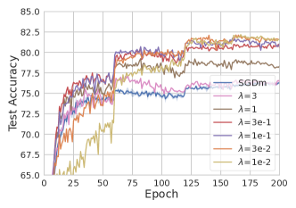
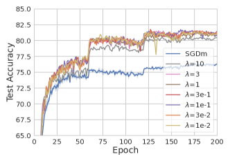
Figure 27: Ablation over (left) $\lambda_{\text{WSD}}$ and (right) $\lambda_{\text{FSD}}$ for training AlexNet on CIFAR-10, using APO-Precond

I.2 Robustness to Initial Learning Rate and Meta-Update Interval

We performed an ablation to evaluate how well APO performs with different meta-update intervals (i.e. when making more or less frequent updates to the learning rate and preconditioning matrix during training). We used APO to tune the learning rate, and experimented with performing meta-updates once every 10, 20, 50, and 100 base optimization iterations. We trained a ResNet32 model on CIFAR-10, and used SGDm as the base optimizer. The results are shown in Figure 29. We found that APO is robust to the meta-update interval, performing almost identically with respect to training loss, test accuracy, and the adaptive learning rate schedule, for each meta-update interval.

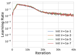
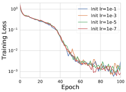
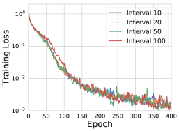
(a)	(b)	(c)

Figure 28: Robustness to the initial learning rate and meta-update interval. Figures (a) and (b) show that APO achieves almost identical learning rate schedules and training losses for initial learning rates spanning 6 orders of magnitude. Figure (c) shows the training loss for ResNet32 on CIFAR-10 using APO with various meta-update intervals—we observe that APO performs similarly using intervals from 10 to 100, corresponding to computation times $1.3\times$ to $1.03\times$ that of the base optimizer.

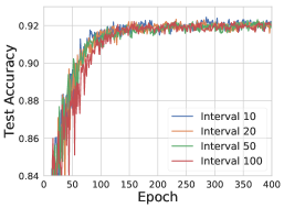
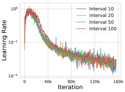
Figure 29: Robustness to the meta update interval. CIFAR-10, SGDm-APO.

To further examine how meta-update intervals affect the preconditioning adaptation, we trained AlexNet model on CIFAR-10. We used APO to learn the preconditioning matrix and experimented with performing meta-updates once every 10, 20, 50, and 100 base optimization iterations. The results are shown in Figure 30. As in the learning rate adaptation problem, we found that APO performs similarly using intervals from 10 to 100, achieving higher test accuracy than the baseline method.

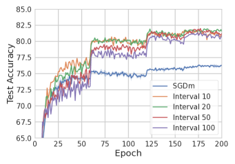
Figure 30: Robustness to the meta update interval on AlexNet. CIFAR-10, APO-Precond.

References

- Amari (1998) Amari, S.-I. Natural gradient works efficiently in learning. Neural Computation, 10(2):251–276, 1998.
- Andrychowicz et al. (2016) Andrychowicz, M., Denil, M., Gomez, S., Hoffman, M. W., Pfau, D., Schaul, T., Shillingford, B., and De Freitas, N. Learning to learn by gradient descent by gradient descent. In Advances in Neural Information Processing Systems, pp. 3981–3989, 2016.
- Arora et al. (2018) Arora, S., Li, Z., and Lyu, K. Theoretical analysis of auto rate-tuning by batch normalization. arXiv preprint arXiv:1812.03981, 2018.
- Asi & Duchi (2019) Asi, H. and Duchi, J. C. Stochastic (approximate) proximal point methods: Convergence, optimality, and adaptivity. SIAM Journal on Optimization, 29(3):2257–2290, 2019.
- Baydin et al. (2017) Baydin, A. G., Cornish, R., Rubio, D. M., Schmidt, M., and Wood, F. Online learning rate adaptation with hypergradient descent. arXiv preprint arXiv:1703.04782, 2017.
- Beck & Teboulle (2003) Beck, A. and Teboulle, M. Mirror descent and nonlinear projected subgradient methods for convex optimization. Operations Research Letters, 31(3):167–175, 2003.
- Becker & Le Cun (1988) Becker, S. and Le Cun, Y. Improving the convergence of back-propagation learning with second order methods. In Proceedings of the 1988 Connecticut Summer School, 1988.
- Belkin et al. (2019) Belkin, M., Hsu, D., Ma, S., and Mandal, S. Reconciling modern machine-learning practice and the classical bias–variance trade-off. Proceedings of the National Academy of Sciences, 116(32):15849–15854, 2019.
- Bengio (2012) Bengio, Y. Practical recommendations for gradient-based training of deep architectures. In Neural Networks: Tricks of the Trade, pp. 437–478. Springer, 2012.
- Benjamin et al. (2018) Benjamin, A. S., Rolnick, D., and Kording, K. Measuring and regularizing networks in function space. arXiv preprint arXiv:1805.08289, 2018.
- Benzing et al. (2019) Benzing, F., Gauy, M. M., Mujika, A., Martinsson, A., and Steger, A. Optimal Kronecker-sum approximation of real time recurrent learning. In International Conference on Machine Learning, pp. 604–613, 2019.
- Bergstra & Bengio (2012) Bergstra, J. and Bengio, Y. Random search for hyper-parameter optimization. Journal of Machine Learning Research, 13(Feb):281–305, 2012.
- Bradbury et al. (2018) Bradbury, J., Frostig, R., Hawkins, P., Johnson, M. J., Leary, C., Maclaurin, D., Necula, G., Paszke, A., VanderPlas, J., Wanderman-Milne, S., and Zhang, Q. JAX: Composable transformations of Python+NumPy programs, 2018. URL http://github.com/google/jax.
- Cettolo et al. (2014) Cettolo, M., Niehues, J., Stüker, S., Bentivogli, L., and Federico, M. Report on the 11th IWSLT evaluation campaign. In Proceedings of the International Workshop on Spoken Language Translation, Hanoi, Vietnam, volume 57, 2014.
- Domke (2012) Domke, J. Generic methods for optimization-based modeling. In Artificial Intelligence and Statistics, pp. 318–326, 2012.
- Donini et al. (2019) Donini, M., Franceschi, L., Pontil, M., Majumder, O., and Frasconi, P. MARTHE: Scheduling the learning rate via online hypergradients. arXiv preprint arXiv:1910.08525, 2019.
- Dua & Graff (2017) Dua, D. and Graff, C. UCI machine learning repository, 2017. URL http://archive.ics.uci.edu/ml.
- Duchi et al. (2011) Duchi, J., Hazan, E., and Singer, Y. Adaptive subgradient methods for online learning and stochastic optimization. Journal of Machine Learning Research, 12(7), 2011.
- Flennerhag et al. (2019) Flennerhag, S., Rusu, A. A., Pascanu, R., Visin, F., Yin, H., and Hadsell, R. Meta-learning with warped gradient descent. arXiv preprint arXiv:1909.00025, 2019.
- Franceschi et al. (2017) Franceschi, L., Donini, M., Frasconi, P., and Pontil, M. Forward and reverse gradient-based hyperparameter optimization. In International Conference on Machine Learning, pp. 1165–1173, 2017.
- George et al. (2018) George, T., Laurent, C., Bouthillier, X., Ballas, N., and Vincent, P. Fast approximate natural gradient descent in a Kronecker-factored eigenbasis. arXiv preprint arXiv:1806.03884, 2018.
- Grosse (2021) Grosse, R. University of Toronto CSC2541, Topics in Machine Learning: Neural Net Training Dynamics, Chapter 4: Second-Order Optimization. Lecture Notes, 2021. URL https://www.cs.toronto.edu/~rgrosse/courses/csc2541_2021/readings/L04_second_order.pdf.
- Grosse & Martens (2016) Grosse, R. and Martens, J. A Kronecker-factored approximate Fisher matrix for convolution layers. In International Conference on Machine Learning, pp. 573–582, 2016.
- Gupta et al. (2018) Gupta, V., Koren, T., and Singer, Y. Shampoo: Preconditioned stochastic tensor optimization. In International Conference on Machine Learning, pp. 1842–1850, 2018.
- Hazan & Kakade (2019) Hazan, E. and Kakade, S. Revisiting the polyak step size. arXiv preprint arXiv:1905.00313, 2019.
- He et al. (2016) He, K., Zhang, X., Ren, S., and Sun, J. Deep residual learning for image recognition. In Conference on Computer Vision and Pattern Recognition, pp. 770–778, 2016.
- Hinton et al. (2015) Hinton, G., Vinyals, O., and Dean, J. Distilling the knowledge in a neural network. arXiv preprint arXiv:1503.02531, 2015.
- Hinton & Salakhutdinov (2006) Hinton, G. E. and Salakhutdinov, R. R. Reducing the dimensionality of data with neural networks. Science, 313(5786):504–507, 2006.
- Ioffe & Szegedy (2015) Ioffe, S. and Szegedy, C. Batch normalization: Accelerating deep network training by reducing internal covariate shift. arXiv preprint arXiv:1502.03167, 2015.
- Jacot et al. (2018) Jacot, A., Gabriel, F., and Hongler, C. Neural tangent kernel: Convergence and generalization in neural networks. arXiv preprint arXiv:1806.07572, 2018.
- Jaderberg et al. (2017) Jaderberg, M., Dalibard, V., Osindero, S., Czarnecki, W. M., Donahue, J., Razavi, A., Vinyals, O., Green, T., Dunning, I., Simonyan, K., et al. Population-based training of neural networks. arXiv preprint arXiv:1711.09846, 2017.
- Jiang et al. (2019) Jiang, H., He, P., Chen, W., Liu, X., Gao, J., and Zhao, T. Smart: Robust and efficient fine-tuning for pre-trained natural language models through principled regularized optimization. arXiv preprint arXiv:1911.03437, 2019.
- Kingma & Ba (2015) Kingma, D. P. and Ba, J. Adam: A method for stochastic optimization. In International Conference on Learning Representations, 2015.
- Krizhevsky et al. (2012) Krizhevsky, A., Sutskever, I., and Hinton, G. E. ImageNet classification with deep convolutional neural networks. In Advances in Neural Information Processing Systems, pp. 1097–1105, 2012.
- Laurent et al. (2018) Laurent, C., George, T., Bouthillier, X., Ballas, N., and Vincent, P. An evaluation of Fisher approximations beyond Kronecker factorization, 2018. URL https://openreview.net/forum?id=ryVC6tkwG.
- Le Roux et al. (2007) Le Roux, N., Manzagol, P.-A., and Bengio, Y. Topmoumoute online natural gradient algorithm. In Advances in Neural Information Processing Systems, pp. 849–856, 2007.
- LeCun (1988) LeCun, Y. The MNIST database of handwritten digits. http://yann. lecun. com/exdb/mnist/, 1988.
- Lee & Choi (2018) Lee, Y. and Choi, S. Gradient-based meta-learning with learned layerwise metric and subspace. In International Conference on Machine Learning, pp. 2927–2936, 2018.
- Li & Malik (2016) Li, K. and Malik, J. Learning to optimize. arXiv preprint arXiv:1606.01885, 2016.
- Li & Malik (2017) Li, K. and Malik, J. Learning to optimize neural nets. arXiv preprint arXiv:1703.00441, 2017.
- Li et al. (2016) Li, L., Jamieson, K., DeSalvo, G., Rostamizadeh, A., and Talwalkar, A. Hyperband: Bandit-based configuration evaluation for hyperparameter optimization. arXiv preprint arXiv:1603.06560, 2016.
- Loizou et al. (2021) Loizou, N., Vaswani, S., Laradji, I. H., and Lacoste-Julien, S. Stochastic polyak step-size for sgd: An adaptive learning rate for fast convergence. In International Conference on Artificial Intelligence and Statistics, pp. 1306–1314. PMLR, 2021.
- Loshchilov & Hutter (2017) Loshchilov, I. and Hutter, F. Decoupled weight decay regularization. arXiv preprint arXiv:1711.05101, 2017.
- Lucas et al. (2019) Lucas, J., Sun, S., Zemel, R., and Grosse, R. Aggregated momentum: Stability through passive damping. In International Conference on Learning Representations, 2019.
- Maclaurin et al. (2015) Maclaurin, D., Duvenaud, D., and Adams, R. Gradient-based hyperparameter optimization through reversible learning. In International Conference on Machine Learning, pp. 2113–2122, 2015.
- Martens (2010) Martens, J. Deep learning via Hessian-free optimization. In International Conference on Machine Learning, 2010.
- Martens (2014) Martens, J. New insights and perspectives on the natural gradient method. arXiv preprint arXiv:1412.1193, 2014.
- Martens (2016) Martens, J. Second-order optimization for neural networks. PhD Thesis. University of Toronto, 2016.
- Martens & Grosse (2015) Martens, J. and Grosse, R. Optimizing neural networks with Kronecker-factored approximate curvature. In International Conference on Machine Learning, pp. 2408–2417, 2015.
- Martens & Sutskever (2011) Martens, J. and Sutskever, I. Learning recurrent neural networks with Hessian-free optimization. In International Conference on Machine Learning, 2011.
- Martens et al. (2018) Martens, J., Ba, J., and Johnson, M. Kronecker-factored curvature approximations for recurrent neural networks. In International Conference on Learning Representations, 2018.
- Metz et al. (2018) Metz, L., Maheswaranathan, N., Nixon, J., Freeman, C. D., and Sohl-Dickstein, J. Learned optimizers that outperform SGD on wall-clock and validation loss. arXiv preprint arXiv:1810.10180, 2018.
- Mishkin et al. (2018) Mishkin, A., Kunstner, F., Nielsen, D., Schmidt, M., and Khan, M. E. Slang: Fast structured covariance approximations for Bayesian deep learning with natural gradient. arXiv preprint arXiv:1811.04504, 2018.
- Moskovitz et al. (2019) Moskovitz, T., Wang, R., Lan, J., Kapoor, S., Miconi, T., Yosinski, J., and Rawal, A. First-order preconditioning via hypergradient descent. arXiv preprint arXiv:1910.08461, 2019.
- Mujika et al. (2018) Mujika, A., Meier, F., and Steger, A. Approximating real-time recurrent learning with random Kronecker factors. arXiv preprint arXiv:1805.10842, 2018.
- Netzer et al. (2011) Netzer, Y., Wang, T., Coates, A., Bissacco, A., Wu, B., and Ng, A. Y. Reading digits in natural images with unsupervised feature learning. In NIPS Workshop on Deep Learning and Unsupervised Feature Learning, 2011.
- Nocedal & Wright (1999) Nocedal, J. and Wright, S. Numerical Optimization. Springer, 1999.
- Ott et al. (2019) Ott, M., Edunov, S., Baevski, A., Fan, A., Gross, S., Ng, N., Grangier, D., and Auli, M. fairseq: A fast, extensible toolkit for sequence modeling. In Proceedings of NAACL-HLT 2019: Demonstrations, 2019.
- Park & Oliva (2019) Park, E. and Oliva, J. B. Meta-curvature. arXiv preprint arXiv:1902.03356, 2019.
- Paszke et al. (2019) Paszke, A., Gross, S., Massa, F., Lerer, A., Bradbury, J., Chanan, G., Killeen, T., Lin, Z., Gimelshein, N., Antiga, L., Desmaison, A., Kopf, A., Yang, E., DeVito, Z., Raison, M., Tejani, A., Chilamkurthy, S., Steiner, B., Fang, L., Bai, J., and Chintala, S. Pytorch: An imperative style, high-performance deep learning library. In Advances in Neural Information Processing Systems 32, pp. 8024–8035. 2019.
- Rahimi & Recht (2017) Rahimi, A. and Recht, B. Reflections on random kitchen sinks, 2017. URL http://www.argmin.net/2017/12/05/kitchen-sinks/.
- Robbins & Monro (1951) Robbins, H. and Monro, S. A stochastic approximation method. The Annals of Mathematical Statistics, pp. 400–407, 1951.
- Rolinek & Martius (2018) Rolinek, M. and Martius, G. L4: Practical loss-based stepsize adaptation for deep learning. In Advances in Neural Information Processing Systems, pp. 6433–6443, 2018.
- Simonyan & Zisserman (2014) Simonyan, K. and Zisserman, A. Very deep convolutional networks for large-scale image recognition. arXiv preprint arXiv:1409.1556, 2014.
- Snoek et al. (2012) Snoek, J., Larochelle, H., and Adams, R. P. Practical Bayesian optimization of machine learning algorithms. In Advances in Neural Information Processing Systems, pp. 2951–2959, 2012.
- Snoek et al. (2015) Snoek, J., Rippel, O., Swersky, K., Kiros, R., Satish, N., Sundaram, N., Patwary, M., Prabhat, P., and Adams, R. Scalable Bayesian optimization using deep neural networks. In International Conference on Machine Learning, pp. 2171–2180, 2015.
- Sutton et al. (2000) Sutton, R. S., McAllester, D. A., Singh, S. P., and Mansour, Y. Policy gradient methods for reinforcement learning with function approximation. In Advances in Neural Information Processing Systems, pp. 1057–1063, 2000.
- Swersky et al. (2014) Swersky, K., Snoek, J., and Adams, R. P. Freeze-thaw Bayesian optimization. arXiv preprint arXiv:1406.3896, 2014.
- Tallec & Ollivier (2017) Tallec, C. and Ollivier, Y. Unbiased online recurrent optimization. arXiv preprint arXiv:1702.05043, 2017.
- Tang et al. (2021) Tang, Z., Jiang, F., Gong, M., Li, H., Wu, Y., Yu, F., Wang, Z., and Wang, M. SKFAC: Training neural networks with faster Kronecker-factored approximate curvature. In Conference on Computer Vision and Pattern Recognition, pp. 13479–13487, 2021.
- Tieleman & Hinton (2012) Tieleman, T. and Hinton, G. Lecture 6.5—RMSprop: Divide the gradient by a running average of its recent magnitude. COURSERA: Neural Networks for Machine Learning, 2012.
- Vaswani et al. (2017) Vaswani, A., Shazeer, N., Parmar, N., Uszkoreit, J., Jones, L., Gomez, A. N., Kaiser, Ł., and Polosukhin, I. Attention is all you need. In Advances in Neural Information Processing Systems, pp. 5998–6008, 2017.
- Vaswani et al. (2019) Vaswani, S., Mishkin, A., Laradji, I., Schmidt, M., Gidel, G., and Lacoste-Julien, S. Painless stochastic gradient: Interpolation, line-search, and convergence rates. In Advances in Neural Information Processing Systems, pp. 3727–3740, 2019.
- Vaswani et al. (2020) Vaswani, S., Laradji, I., Kunstner, F., Meng, S. Y., Schmidt, M., and Lacoste-Julien, S. Adaptive gradient methods converge faster with over-parameterization (but you should do a line-search). arXiv preprint arXiv:2006.06835, 2020.
- Vicol et al. (2021) Vicol, P., Metz, L., and Sohl-Dickstein, J. Unbiased gradient estimation in unrolled computation graphs with persistent evolution strategies. In International Conference on Machine Learning, pp. 10553–10563, 2021.
- Wadia et al. (2021) Wadia, N., Duckworth, D., Schoenholz, S. S., Dyer, E., and Sohl-Dickstein, J. Whitening and second order optimization both make information in the dataset unusable during training, and can reduce or prevent generalization. In International Conference on Machine Learning, pp. 10617–10629, 2021.
- Wichrowska et al. (2017) Wichrowska, O., Maheswaranathan, N., Hoffman, M. W., Colmenarejo, S. G., Denil, M., de Freitas, N., and Sohl-Dickstein, J. Learned optimizers that scale and generalize. In International Conference on Machine Learning, pp. 3751–3760, 2017.
- Wu et al. (2018) Wu, Y., Ren, M., Liao, R., and Grosse, R. Understanding short-horizon bias in stochastic meta-optimization. In International Conference on Learning Representations, 2018.
- Zagoruyko & Komodakis (2016) Zagoruyko, S. and Komodakis, N. Wide residual networks. arXiv preprint arXiv:1605.07146, 2016.
- Zhang et al. (2019a) Zhang, G., Li, L., Nado, Z., Martens, J., Sachdeva, S., Dahl, G., Shallue, C., and Grosse, R. B. Which algorithmic choices matter at which batch sizes? insights from a noisy quadratic model. Advances in neural information processing systems, 32:8196–8207, 2019a.
- Zhang et al. (2019b) Zhang, G., Martens, J., and Grosse, R. Fast convergence of natural gradient descent for overparameterized neural networks. arXiv preprint arXiv:1905.10961, 2019b.