An Empirical Study on Explanations in Out-of-Domain Settings
Abstract
Recent work in Natural Language Processing has focused on developing approaches that extract faithful explanations, either via identifying the most important tokens in the input (i.e. post-hoc explanations) or by designing inherently faithful models that first select the most important tokens and then use them to predict the correct label (i.e. select-then-predict models). Currently, these approaches are largely evaluated on in-domain settings. Yet, little is known about how post-hoc explanations and inherently faithful models perform in out-of-domain settings. In this paper, we conduct an extensive empirical study that examines: (1) the out-of-domain faithfulness of post-hoc explanations, generated by five feature attribution methods; and (2) the out-of-domain performance of two inherently faithful models over six datasets. Contrary to our expectations, results show that in many cases out-of-domain post-hoc explanation faithfulness measured by sufficiency and comprehensiveness is higher compared to in-domain. We find this misleading and suggest using a random baseline as a yardstick for evaluating post-hoc explanation faithfulness. Our findings also show that select-then predict models demonstrate comparable predictive performance in out-of-domain settings to full-text trained models.111Code available at: https://github.com/GChrysostomou/ood_faith
1 Introduction
An explanation or rationale222We use these terms interchangeably throughout our work., typically consists of a subset of the input that contributes more to the prediction. Extracting faithful explanations is important for studying model behavior (Adebayo et al., 2020) and assisting in tasks requiring human decision making, such as clinical text classification (Chakrabarty et al., 2019), misinformation detection (Popat et al., 2018; Mu and Aletras, 2020) and legal text classification (Chalkidis et al., 2019, 2021). A faithful explanation is one which accurately represents the reasoning behind a model’s prediction (Jacovi and Goldberg, 2020)
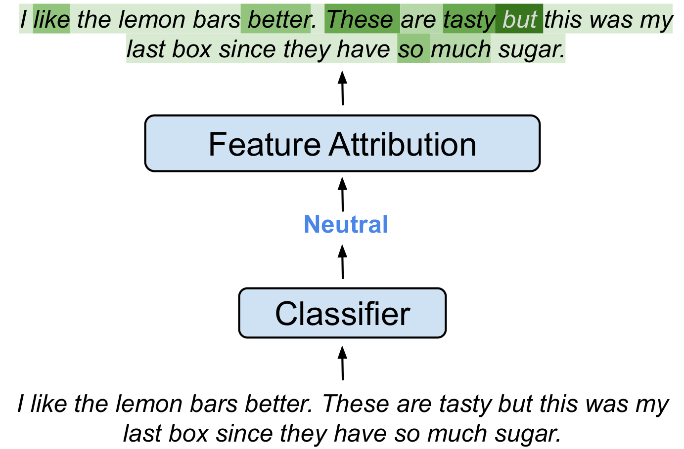
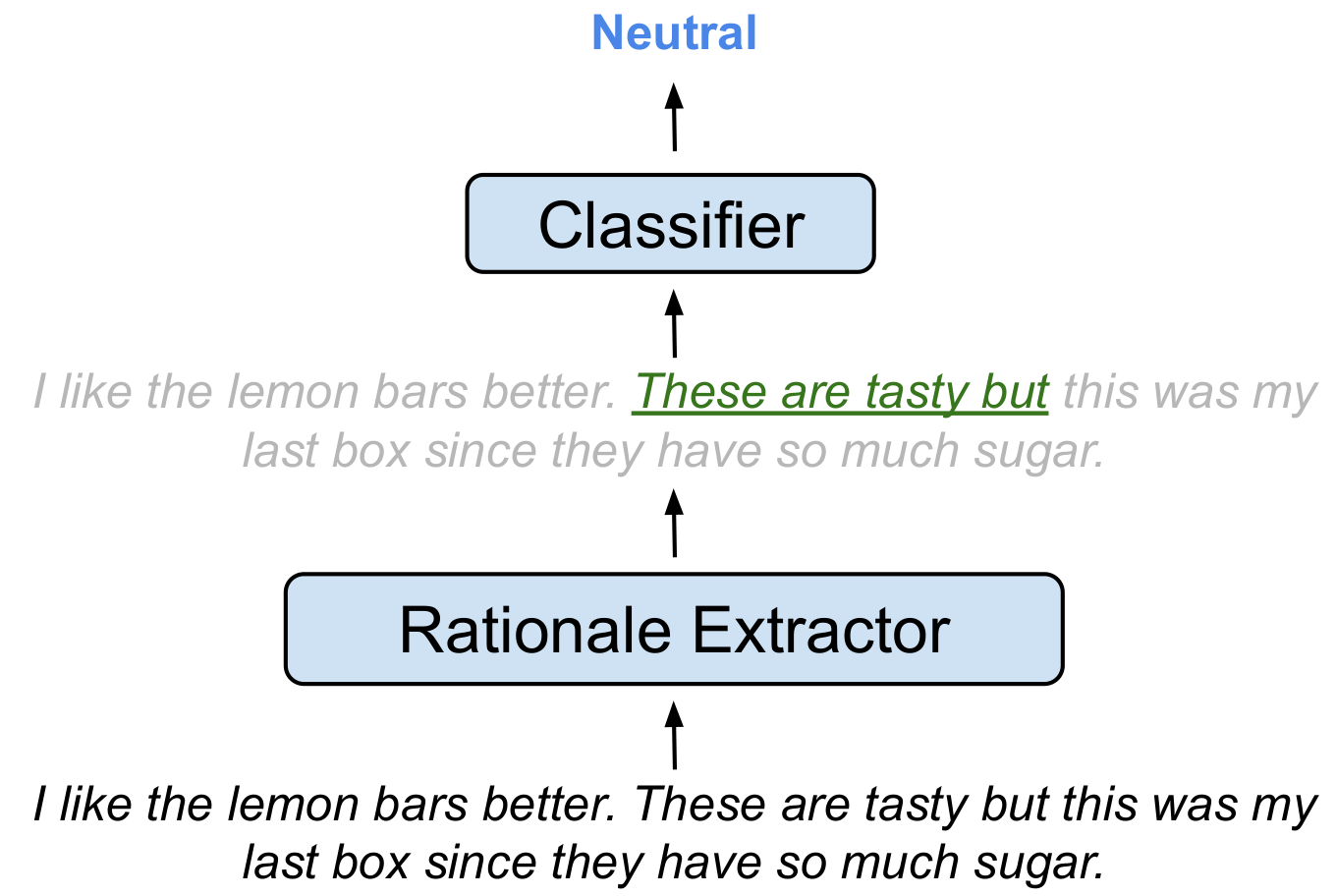
Two popular methods for extracting explanations are through feature attribution approaches (i.e. post-hoc explanation methods) or via inherently faithful classifiers (i.e. select-then-predict models). The first computes the contribution of different parts of the input with respect to a model’s prediction (Sundararajan et al., 2017; Ribeiro et al., 2016; Shrikumar et al., 2017). The latter consists of using a rationale extractor to identify the most important parts of the input and a rationale classifier, a model trained using as input only the extractor’s rationales (Bastings et al., 2019; Jain et al., 2020; Guerreiro and Martins, 2021).333We refer to the rationale generator (i.e. generating a rationale mask) from Bastings et al. (2019) and Jain et al. (2020) as a rationale extractor, to avoid any confusion between these approaches and free-text rationales (Wiegreffe et al., 2021). Figure 1 illustrates the two approaches with an example.
Currently, these explanation methods have been mostly evaluated on in-domain settings (i.e. the train and test data come from the same distribution). However, when deploying models in real-world applications, inference might be performed on data from a different distribution, i.e. out-of-domain (Desai and Durrett, 2020; Ovadia et al., 2019). This can create implications when extracted explanations (either using post-hoc methods or through select-then-predict models) are used for assisting human decision making. Whilst we are aware of the limitations of current state-of-the-art models in out-of-domain predictive performance (Hendrycks et al., 2020), to the best of our knowledge, how faithful out-of-domain post-hoc explanations are has yet to be explored. Similarly, we are not aware how inherently faithful select-then-predict models generalize in out-of-domain settings.
Inspired by this, we conduct an extensive empirical study to examine the faithfulness of five feature attribution approaches and the generalizability of two select-then-predict models in out-of-domain settings across six dataset pairs. We hypothesize that similar to model predictive performance, post-hoc explanation faithfulness reduces in out-of-domain settings and that select-then-predict performance degrades. Our contributions are as follows:
-
•
To the best of our knowledge, we are the first to assess the faithfulness of post-hoc explanations and performance of select-then-predict models in out-of-domain settings.
-
•
We show that post-hoc explanation sufficiency and comprehensiveness show misleading increases in out-of-domain settings. We argue that they should be evaluated alongside a random baseline as yardstick out-of-domain.
-
•
We demonstrate that select-then-predict classifiers can be used in out-of-domain settings. They lead to comparable predictive performance to models trained on full-text, whilst offering inherent faithfulness.
2 Related Work
2.1 Rationale Extraction
Given a model , we are interested in explaining why predicted for a particular instance . An extracted rationale , should therefore represent as accurately as possible the most important subset of the input () which contributed mostly towards the model’s prediction .
Currently, there are two popular approaches for extracting rationales. The first consists of using feature attribution methods that attribute to the input tokens an importance score (i.e. how important an input token is to a model’s prediction ). We can then form a rationale , by selecting the most important tokens (independent or contiguous) as indicated by the feature attribution method. The second select-then-predict approach focuses on training inherently faithful classifiers by jointly training two modules, a rationale extractor and a rationale classifier, trained only on rationales produced by the extractor (Lei et al., 2016; Bastings et al., 2019; Treviso and Martins, 2020; Jain et al., 2020; Guerreiro and Martins, 2021). Recent studies have used feature attribution approaches as part of the rationale extractor (Jain et al., 2020; Treviso and Martins, 2020), showing improved classifier predictive performance.
2.2 Evaluating Rationale Faithfulness
Having extracted , we need to evaluate the quality of the explanation (i.e. how faithful that explanation is for a model’s prediction). Typically, post-hoc explanations from feature attribution approaches are evaluated using input erasure (Serrano and Smith, 2019; Atanasova et al., 2020; Madsen et al., 2021). This approach masks segments of the input to observe if the model’s prediction changed. DeYoung et al. (2020) proposed measuring the comprehensiveness and sufficiency of rationales as faithfulness metrics. A comprehensive rationale is one which is influential to a model’s prediction, while a sufficient rationale that which is adequate for a model’s prediction (DeYoung et al., 2020). The term fidelity is also used for jointly referring to comprehensiveness and sufficiency (Carton et al., 2020). Carton et al. (2020) suggested normalizing these metrics using the predictions of the model with a baseline input (i.e. an all zero embedding vector), to account for baseline model behavior. Select-then-predict models are inherently faithful, as their classification component is trained only on extracted rationales (Jain et al., 2020). A good measure for measuring rationale quality is by evaluating the predictive performance of the classifier trained only on the rationales Jain et al. (2020); Treviso and Martins (2020). A higher score entails that the extracted rationales are better when compared to those of a classifier with lower predictive performance.
2.3 Explainability in Out-of-Domain Settings
Given model trained on an end-task, we typically evaluate its out-of-domain predictive performance on a test-set that does not belong to the same distribution as the data it was trained on (Hendrycks et al., 2020). Similarly, the model can also extract explanations for its out-of-domain predictions.
Camburu et al. (2018) studied whether generating explanations for language inference match human annotations (i.e. plausible explanations). They showed that this is challenging in-domain and becomes more challenging in out-of-domain settings. In a similar direction, Rajani et al. (2019) and Kumar and Talukdar (2020) examined model generated explanations in out-of-domain settings and find that explanation plausibility degrades compared to in-domain. Kennedy et al. (2020) proposed a method for detecting model bias towards group identity terms using a post-hoc feature attribution approach. Then, they use them for regularizing models to improve out-of-domain predictive performance. Adebayo et al. (2020) have studied feature attribution approaches for identifying out-of-distribution images. They find that importance allocation in out-of-domain settings is similar to that of an in-domain model and thus cannot be used to detect such images. Feder et al. (2021) finally argued that explanations can lead to errors in out-of-distribution settings, as they may latch onto spurious features from the training distribution.
These studies indicate that there is an increasing need for evaluating post-hoc explanation faithfulness and select-then-predict performance in out-of-domain settings. To the best of our knowledge, we are the first to examine these.
3 Extracting Rationales
3.1 Post-hoc Explanations
We employ a pre-trained BERT-base and fine-tune it on in-domain training data. We then extract post-hoc rationales for both the in-domain test-set and two out-of-domain test-sets. We compute input importance using five feature scoring methods and a random baseline:
-
•
Random (Rand): Random allocation of token importance.
-
•
Attention (): Token importance corresponding to normalized attention scores Jain et al. (2020).
-
•
Scaled Attention (): Attention scores scaled by their corresponding gradients Serrano and Smith (2019).
- •
-
•
Integrated Gradients (): Ranking words by computing the integral of the gradients taken along a straight path from a baseline input (zero embedding vector) to the original input Sundararajan et al. (2017).
-
•
DeepLift: Ranking words according to the difference between the activation of each neuron and a reference activation (zero embedding vector) Shrikumar et al. (2017).
3.2 Select-then-Predict Models
We use two select-then-predict models:
-
•
HardKuma: An end-to-end trained model, where the rationale extractor uses Hard Kumaraswamy variables to produce a rationale mask z, which the classifier uses to mask the input (Bastings et al., 2019). Model training takes advantage of reparameterized gradients compared to REINFORCE style training employed by Lei et al. (2016) and has shown improved performance (Guerreiro and Martins, 2021).
-
•
FRESH: We compute the predictive performance of a classifier trained on rationales extracted with feature attribution metrics (see 3.1) using FRESH, following a similar approach to Jain et al. (2020). We extract rationales from an extractor by (1) selecting the top- most important tokens (TopK) and (2) selecting the span of length with the highest overall importance (Contiguous).
We use BERT-base for the extraction and classification components of FRESH similar to Jain et al. (2020). However, for HardKuma we opt using a bi-LSTM (Hochreiter and Schmidhuber, 1997) as it provides comparable or improved performance over BERT variants (Guerreiro and Martins, 2021), even after hyperparameter tuning.444See model details and hyper-parameters in Appendix B
4 Experimental Setup
4.1 Datasets
For evaluating out-of-domain model explanation, we consider the following datasets (see Table 1 and Appendix A for details):
SST:
Stanford Sentiment Treebank (SST) consists of sentences tagged with sentiment on a 5-point-scale from negative to positive (Socher et al., 2013). We remove sentences with neutral sentiment and label the remaining sentences as negative or positive if they have a score lower or higher than 3 respectively (Jain and Wallace, 2019).
IMDB:
Yelp:
Yelp polarity review texts. Similar to Zhang et al. (2015) we construct a binary classification task to predict a polarity label by considering one and two stars as negative, and three and four stars as positive.
Amazon Reviews:
We form 3-way classification tasks by predicting the sentiment (negative, neutral, positive) of Amazon product reviews across 3 item categories: (1) Digital Music (AmazDigiMu); (2) Pantry (AmazPantry); and (3) Musical Instruments (AmazInstr) (Ni et al., 2019).
| Dataset | C | Splits |
|---|---|---|
| SST | 2 | 6,920 / 872 / 1,821 |
| IMDB | 2 | 20,000 / 2,500 / 2,500 |
| Yelp | 2 | 476,000 / 84,000 / 38,000 |
| AmazDigiMu | 3 | 122,552 / 21,627 / 25,444 |
| AmazPantry | 3 | 99,423/ 17,546 / 20,642 |
| AmazInstr | 3 | 167,145 / 29,497 / 34,702 |
4.2 Evaluating Out-of-Domain Explanations
Post-hoc Explanations:
We evaluate post-hoc explanations using:
| Train | Test | Full-text | Normalized Sufficiency | Normalized Comprehensiveness | ||||||||||
|---|---|---|---|---|---|---|---|---|---|---|---|---|---|---|
| F1 | Rand | DeepLift | IG | Rand | DeepLift | IG | ||||||||
| SST | SST | 90.1 | 0.38 | 0.51 | 0.42 | 0.42 | 0.40 | 0.41 | 0.19 | 0.39 | 0.22 | 0.25 | 0.26 | 0.26 |
| IMDB | 84.3 | 0.31 | 0.53 | 0.39 | 0.32 | 0.31 | 0.32 | 0.23 | 0.54 | 0.34 | 0.27 | 0.27 | 0.28 | |
| Yelp | 87.9 | 0.32 | 0.56 | 0.40 | 0.35 | 0.33 | 0.34 | 0.21 | 0.48 | 0.28 | 0.24 | 0.24 | 0.25 | |
| IMDB | IMDB | 91.1 | 0.32 | 0.55 | 0.46 | 0.36 | 0.36 | 0.36 | 0.16 | 0.48 | 0.31 | 0.25 | 0.23 | 0.24 |
| SST | 85.8 | 0.24 | 0.35 | 0.28 | 0.28 | 0.27 | 0.27 | 0.27 | 0.46 | 0.32 | 0.33 | 0.33 | 0.33 | |
| Yelp | 91.0 | 0.35 | 0.48 | 0.41 | 0.36 | 0.36 | 0.36 | 0.21 | 0.45 | 0.32 | 0.26 | 0.26 | 0.26 | |
| Yelp | Yelp | 96.9 | 0.23 | 0.32 | 0.31 | 0.29 | 0.24 | 0.25 | 0.12 | 0.20 | 0.14 | 0.16 | 0.15 | 0.16 |
| SST | 86.8 | 0.41 | 0.45 | 0.43 | 0.44 | 0.41 | 0.41 | 0.17 | 0.24 | 0.18 | 0.21 | 0.22 | 0.22 | |
| IMDB | 88.6 | 0.18 | 0.34 | 0.32 | 0.25 | 0.22 | 0.22 | 0.19 | 0.34 | 0.29 | 0.23 | 0.23 | 0.24 | |
| AmazDigiMu | AmazDigiMu | 70.6 | 0.34 | 0.56 | 0.34 | 0.31 | 0.41 | 0.39 | 0.13 | 0.32 | 0.14 | 0.10 | 0.16 | 0.17 |
| AmazInstr | 61.2 | 0.29 | 0.54 | 0.32 | 0.31 | 0.33 | 0.32 | 0.19 | 0.47 | 0.23 | 0.19 | 0.22 | 0.23 | |
| AmazPantry | 64.6 | 0.33 | 0.55 | 0.33 | 0.31 | 0.37 | 0.36 | 0.21 | 0.46 | 0.22 | 0.17 | 0.23 | 0.25 | |
| AmazPantry | AmazPantry | 70.2 | 0.25 | 0.46 | 0.36 | 0.19 | 0.28 | 0.27 | 0.20 | 0.42 | 0.31 | 0.15 | 0.25 | 0.25 |
| AmazDigiMu | 59.5 | 0.24 | 0.47 | 0.37 | 0.19 | 0.27 | 0.26 | 0.19 | 0.41 | 0.32 | 0.15 | 0.23 | 0.24 | |
| AmazInstr | 64.5 | 0.17 | 0.42 | 0.30 | 0.15 | 0.20 | 0.20 | 0.24 | 0.52 | 0.40 | 0.23 | 0.30 | 0.30 | |
| AmazInstr | AmazInstr | 71.5 | 0.16 | 0.34 | 0.18 | 0.21 | 0.18 | 0.17 | 0.26 | 0.52 | 0.26 | 0.29 | 0.28 | 0.29 |
| AmazDigiMu | 61.3 | 0.21 | 0.38 | 0.21 | 0.22 | 0.24 | 0.22 | 0.23 | 0.46 | 0.20 | 0.22 | 0.24 | 0.25 | |
| AmazPantry | 68.2 | 0.22 | 0.39 | 0.21 | 0.23 | 0.24 | 0.23 | 0.27 | 0.51 | 0.22 | 0.25 | 0.27 | 0.29 | |
-
•
Normalized Sufficiency (NormSuff) measures the degree to which the extracted rationales are adequate for a model to make a prediction DeYoung et al. (2020). Following Carton et al. (2020), we bind sufficiency between 0 and 1 and use the reverse difference so that higher is better:
(1) where is the sufficiency of a baseline input (zeroed out sequence) and the model predicted class using the full text as input.
-
•
Normalized Comprehensiveness (NormComp) measures the influence of a rationale to a prediction DeYoung et al. (2020). For an explanation to be highly comprehensive, the model’s prediction after masking the rationale should have a large difference compared to the model’s prediction using the full text. Similarly to Carton et al. (2020), we bind this metric between 0 and 1 and normalize it:
(2)
To measure sufficiency and comprehensiveness across different explanation lengths we compute the “Area Over the Perturbation Curve" (AOPC) following DeYoung et al. (2020). We therefore compute and report the average normalized sufficiency and comprehensiveness scores when keeping (for sufficiency) or masking (for comprehensiveness) the top 2%, 10%, 20% and 50% of tokens extracted by an importance attribution function.555We also present results for each of these rationale lengths in Appendix F.
We omit from our evaluation the Remove-and-Retrain method (Madsen et al., 2021) as it requires model retraining. Whilst this could be applicable for in-domain experiments where retraining is important, in this work we evaluate explanation faithfulness in zero-shot out-of-domain settings.
Select-then-Predict Models:
We first train select-then-predict models in-domain and then measure their predictive performance on the in-domain test-set and on two out-of-domain test-sets (Jain et al., 2020; Guerreiro and Martins, 2021). Our out-of-domain evaluation is performed without re-training (zero-shot). Similar to full-text trained models, we expect that predictive performance deteriorates out-of-domain. However, we assume that explanations from a select-then-predict model should generalize better in out-of-domain settings when the predictive performance approaches that of the full-text trained model.
5 Results
5.1 Post-hoc Explanation Faithfulness
Table 2 presents the normalized comprehensiveness and sufficiency scores for post-hoc explanations on in-domain and out-of-domain test-sets, using five feature attribution methods and a random baseline. For reference, we include the averaged F1 performance across 5 random seeds, of a BERT-base model finetuned on the full text and evaluated in- and out-of-domain (Full-text F1).666We report predictive performance for all models and standard deviations in the Appendix.
In-domain results show that feature attribution performance varies largely across datasets. This is in line with the findings of Atanasova et al. (2020) and Madsen et al. (2021) when masking rationales (i.e. comprehensiveness). We find the only exception to be , which consistently achieves the highest comprehensiveness and sufficiency scores across all in-domain datasets. For example evaluated on in-domain AmazDigiMu, results in sufficiency of 0.56 compared to the second best of 0.39 with IG.
Contrary to our expectations, results show that post-hoc explanation sufficiency and comprehensiveness are in many cases higher in out-of-domain test-sets compared to in-domain. For example using DeepLift, comprehensiveness for the in-domain test-set in Yelp (0.16) is lower compared to the out-of-domain test-sets (0.21 for SST and 0.23 for IMDB). This is also observed when measuring sufficiency with , scoring 0.32 when tested in-domain on Yelp and 0.45 for the out-of-domain SST test-set.
Apart from increased sufficiency and comprehensiveness scores in out-of-domain post-hoc explanations, we also observe increased scores obtained by our random baseline. In fact, the random baseline outperforms several feature attribution approaches in certain cases in out-of-domain settings . As an example, consider the case where the model has been trained on AmazInstr and tested on AmazPantry. Our random baseline achieves a comprehensiveness score of 0.27 while , DeepLift, perform similarly or lower (0.22, 0.25 and 0.27 respectively). Similarly, using a model trained on Yelp and tested on SST, the random baseline produces equally sufficient rationales to and IG, with all of them achieving 0.41 normalized sufficiency. A glaring exception to this pattern is , which consistently outperforms both the random baseline and all other feature attribution approaches in in- and out-of-domain settings, suggesting that it produces the more faithful explanations. For example with out-of-domain AmazPantry test data, using a model trained on AmazInstr results in sufficiency scores of 0.39 with . This is a 0.15 point increase compared to the second best ( with 0.24).
We recommend considering a feature attribution for producing faithful explanations out-of-domain, if it only scores above a baseline random attribution. We suggest that the higher the deviation from the random baseline, the more faithful an explanation is.
| Train | Test | Full-text | HardKuma | L |
|---|---|---|---|---|
| F1 | F1 | (%) | ||
| SST | SST | 81.7 | 77.6 | 56.8 |
| IMDB | 71.9 | 65.7 | 39.5 | |
| Yelp | 68.7 | 67.7 | 32.7 | |
| IMDB | IMDB | 87.4 | 82.0 | 1.9 |
| SST | 77.5 | 73.6 | 16.8 | |
| Yelp | 41.0 | 47.2 | 3.1 | |
| Yelp | Yelp | 96.0 | 92.4 | 7.4 |
| SST | 80.4 | 72.4 | 14.1 | |
| IMDB | 84.5 | 73.3 | 4.7 | |
| AmazDigiMu | AmazDigiMu | 67.6 | 66.8 | 18.4 |
| AmazInstr | 54.2 | 53.3 | 25.8 | |
| AmazPantry | 55.3 | 54.7 | 27.8 | |
| AmazPantry | AmazPantry | 67.9 | 66.6 | 18.9 |
| AmazDigiMu | 50.9 | 51.0 | 11.2 | |
| AmazInstr | 55.9 | 57.4 | 18.2 | |
| AmazInstr | AmazInstr | 67.2 | 66.7 | 19.2 |
| AmazDigiMu | 54.3 | 53.7 | 13.9 | |
| AmazPantry | 61.1 | 59.5 | 24.4 |
| Train | Test | Full-text | DeepLift | IG | |||
|---|---|---|---|---|---|---|---|
| SST (20%) | SST | 90.1 | 87.7 | 81.1 | 84.4 | 76.3 | 76.8 |
| IMDB | 84.3 | 81.8 | 52.6 | 64.0 | 55.0 | 56.3 | |
| Yelp | 87.9 | 88.1 | 72.6 | 75.4 | 59.6 | 63.9 | |
| IMDB (2%) | IMDB | 91.1 | 87.9 | 80.4 | 87.2 | 59.8 | 59.7 |
| SST | 85.8 | 80.9 | 71.8 | 70.1 | 69.6 | 70.7 | |
| Yelp | 91.0 | 87.8 | 82.0 | 79.4 | 69.0 | 69.1 | |
| Yelp (10%) | Yelp | 96.9 | 94.0 | 90.4 | 93.6 | 70.5 | 71.9 |
| SST | 86.8 | 59.3 | 69.8 | 67.2 | 67.7 | 69.3 | |
| IMDB | 88.6 | 78.0 | 64.5 | 66.6 | 53.0 | 55.8 | |
| AmazDigiMu (20%) | AmazDigiMu | 70.6 | 66.1 | 63.4 | 65.8 | 51.9 | 65.8 |
| AmazInstr | 61.2 | 58.0 | 57.2 | 57.4 | 46.0 | 57.2 | |
| AmazPantry | 64.6 | 59.1 | 56.5 | 56.5 | 44.8 | 44.8 | |
| AmazPantry (20%) | AmazPantry | 70.2 | 67.3 | 62.6 | 67.2 | 48.6 | 48.7 |
| AmazDigiMu | 59.5 | 57.7 | 54.6 | 56.2 | 41.2 | 57.7 | |
| AmazInstr | 64.5 | 63.8 | 58.0 | 63.6 | 40.1 | 40.3 | |
| AmazInstr (20%) | AmazInstr | 71.5 | 69.8 | 62.1 | 69.7 | 45.6 | 48.6 |
| AmazDigiMu | 61.3 | 60.0 | 53.2 | 57.8 | 43.8 | 60.0 | |
| AmazPantry | 68.2 | 64.5 | 56.3 | 63.1 | 44.6 | 47.6 |
5.2 Select-then-predict Model Performance
HardKuma:
Table 3 presents the F1-macro performance of HardKuma models (Bastings et al., 2019) and the average rationale lengths (the ratio of the selected tokens compared to the length of the entire sequence) selected by the model. For reference, we also include the predictive performance of a full-text trained bi-LSTM. Results are averaged across 5 runs including standard deviations in brackets.
As expected, predictive performance of HardKuma models degrades when evaluated on out-of-domain data. Surprisingly, though, we find that their performance is not significantly different (t-test; p-value 0.05) to that of the full-text LSTM in 9 out of the 12 out-of-domain dataset pairs. For example, by evaluating the out-of-domain performance of a HardKuma model trained on AmazDigiMu on the AmazPantry test-set, we record on average a score of 54.3 F1 compared to 55.3 with an LSTM classifier trained on full text. We also observe that HardKuma models trained on SST and IMDB generalize comparably to models trained on full-text when evaluated on Yelp, however the opposite does not apply. Our assumption is that HardKuma models trained on Yelp, learn more domain-specific information due to the large training corpus (when compared to training on IMDB and SST) so they fail to generalize well out-of-domain.
Results also show, that the length of rationales selected by HardKuma models depend on the source domain, i.e. training HardKuma on a dataset which favors shorter rationales, leads to also selecting shorter rationales out-of-domain. For example, in-domain test-set explanation lengths are on average 56.8% of the full-text input length for SST. In comparison, training a model on Yelp and evaluating on SST results in rationale lengths of 14.1%. We observe that in certain cases, HardKuma models maintain the number of words, not the ratio to the sequence in out-of-domain settings. For example, in-domain Yelp test-set rationales are about 11 tokens long that is the similar to the length selected when evaluating on IMDB using a model trained on Yelp. This is also observed where in-domain AmazInstr test-set rationales are on average 5 tokens long, which is the same rationale length when evaluating on AmazDigiMu using a model trained on AmazInstr.
In general, our findings show that in the majority of cases, using HardKuma in out-of-domain data results to comparable performance with their full-text model counterparts. This suggests that HardKuma models can be used in out-of-domain settings, without significant sacrifices in predictive performance whilst also offering faithful rationales.
FRESH:
Table 4 shows the averaged F1-macro performance across 5 random seeds for FRESH classifiers on in- and out-of-domain using TopK rationales.777For clarity we include standard deviations and Contiguous results in Appendix D. We also include the a priori defined rationale length in parentheses and the predictive performance of the Full-Text model for reference.888When evaluating out-of-domain, we use the average rationale length of the dataset we evaluate on. This makes FRESH experiments comparable with those of HardKuma.
We first observe that in-domain predictive performance varies across feature attribution approaches with attention-based metrics (, ) outperforming the gradient-based ones (, IG), largely agreeing with Jain et al. (2020). We also find that and DeepLift are the feature attribution approaches that lead to the highest predictive performance across all datasets.
As we initially hypothesized, performance of FRESH generally degrades when testing on out-of-domain data similarly to the behavior of models trained using the full text. The only exceptions are when using and IG in IMDB. We argue that this is due to these feature attribution methods not being able to identify the appropriate tokens relevant to the task using a rationale length 2% of the original input. Increasing the rationale length to 20% (SST) and 10% (Yelp) also increases the performance. Results also suggest that and DeepLift outperform the rest of the feature attributions, with being the best performing one in the majority of cases. In fact when using or DeepLift, the out-of-domain performance of FRESH is not significantly different to that of models trained on full text (t-test; p-value 0.05) in 5 cases. For example, a FRESH model trained on AmazPantry and evaluated on AmazInstr records 63.6 F1 macro (using DeepLift) compared to 64.5 obtained by a full-text model. However, this does not apply to the other feature attribution methods (; ; IG).
To better understand this behavior, we conduct a correlation analysis between the importance rankings using any single feature attribution from (1) a model trained on the same domain with the evaluation data; and (2) a model trained on a different domain (out-of-domain trained model). High correlations suggest that if a feature attribution from an out-of-domain trained model produces similar importance distributions with that of an in-domain model, it will also lead to high predictive performance out-of-domain. Contrary to our initial assumption we found that the lower the correlation, the higher the predictive performance with FRESH. Results show low correlations when using and DeepLift (highest FRESH performance). Surprisingly, IG and (lowest FRESH performance) showed consistently strong correlations across all dataset pairs. Thus, we conclude that lower correlation scores indicate lower attachment to spurious correlations learned during training. We expand our discussion and show results for the correlation analysis in Appendix E.
Our findings therefore suggest that using FRESH in out-of-domain settings, can result to comparable performance with a model trained on full-text. However this highly depends on the choice of the feature attribution method.
HardKuma vs. FRESH:
We observe that HardKuma models are not significantly different compared to models trained on the full text in out-of-domain settings in more cases, when compared to FRESH (9 out of 12 and 5 out of 12 respectively). However, FRESH with or DeepLift records higher predictive performance compared to HardKuma models (both in- and out-of-domain) in all cases. We attribute this to the underlying model architectures, as FRESH uses BERT and HardKuma a bi-LSTM. As we discussed in §3.2, we attempted using BERT for HardKuma models in the extractor and classifier similar to Jain et al. (2020). However, the performance of HardKuma with BERT is at most comparable to when using a bi-LSTM similar to findings of Guerreiro and Martins (2021).
5.3 Correlation between Post-hoc Explanation Faithfulness and FRESH Performance
We hypothesize that a feature attribution with high scores for sufficiency and comprehensiveness, should extract rationales that result in high FRESH predictive performance. We expect that if our hypothesis is valid, faithfulness scores can serve as early indicators of FRESH performance, both on in-domain and out-of-domain settings.
Table 5 shows the Spearman’s ranking correlation () between FRESH F1 performance (see Table 4) and comprehensiveness and sufficiency (see Table 2). Correlation is computed using all feature scoring methods for each dataset pair. Results show that only 4 cases achieve statistically significant correlations (p-value 0.05) with only 3 out-of-domain and mostly between sufficiency and FRESH performance. We do not observe high correlations with comprehensiveness which is expected, as comprehensiveness evaluated the rationale’s influence towards a model’s prediction. Our findings refute our initial hypothesis and suggest that there is no clear correlation across all cases, between post-hoc explanation faithfulness and FRESH predictive performance. Therefore, sufficiency and comprehensiveness scores cannot be used as early indicators of FRESH predictive performance.
| Train | Test | ||
|---|---|---|---|
| FRESH | Sufficiency | Comprehen. | |
| SST | SST | 0.97 | 0.15 |
| IMDB | 0.36 | 0.21 | |
| Yelp | 0.90 | 0.56 | |
| IMDB | IMDB | 0.69 | 0.87 |
| SST | 0.65 | 0.23 | |
| Yelp | 0.92 | 0.92 | |
| Yelp | Yelp | 0.82 | 0.55 |
| SST | -0.67 | -0.67 | |
| IMDB | 0.87 | 0.56 | |
| AmazDigiMu | AmazDigiMu | -0.11 | 0.22 |
| AmazInstr | 0.23 | 0.69 | |
| AmazPantry | 0.11 | 0.11 | |
| AmazPantry | AmazPantry | 0.16 | 0.16 |
| AmazDigiMu | 0.05 | 0.41 | |
| AmazInstr | 0.16 | 0.16 | |
| AmazInstr | AmazInstr | 0.79 | 0.55 |
| AmazDigiMu | 0.24 | 0.67 | |
| AmazPantry | 0.21 | 0.20 | |
6 Qualitative Analysis
Table 6 presents examples from a qualitative analysis we performed, aimed at better understanding out-of-domain post-hoc explanations. Rows with highlighted text in blue are from a model trained in the same domain as the presented example (ID), whilst those with highlighted text in red are from models trained on a different domain. Importance scores are computed using scaled attention ().
| Trained On | Example | |
|---|---|---|
| (1) | AmazInstr (ID) | Work great and sound good |
| AmazDigiMu | Work great and sound good | |
| AmazPantry | Work great and sound good | |
| (2) | AmazPantry (ID) | Delicious and at a good price . would recommend . |
| AmazDigiMu | Delicious and at a good price . would recommend . | |
| AmazInstr | Delicious and at a good price . would recommend . | |
| (3) | SST (ID) | A painfully funny ode to bad behavior |
| IMDB | A painfully funny ode to bad behavior | |
| Yelp | A painfully funny ode to bad behavior | |
| (4) | Yelp (ID) | The kouign - amann is so amazing … must taste to appreciate . |
| SST | The kouign - amann is so amazing … must taste to appreciate . | |
| IMDB | The kouign - amann is so amazing … must taste to appreciate . | |
In Example (1), we observe that models trained on two closely related tasks (AmazInstr and AmazDigiMu) place more importance to the phrase “sound good”. On the contrary, the model trained on AmazPantry which has not encountered such phrases during training, mostly focuses on “Work great”. This is expected as the term “sound” is not typical of pantry reviews. Similarly, in Example (2) from the AmazPantry dataset, the in-domain model focuses on a domain-specific word “delicious”. On the contrary, the two models trained on music-related tasks focus on more generic terms such as “good” and “would recommend”. In Example (3) the model trained on Yelp focuses mostly on the word “behavior”, a term we consider more relevant to restaurant reviews rather than movie reviews. In comparison, the other models which are both trained on movie reviews focus both on the term “funny”. In Example (4), again the two movie-review models focus on more generic terms (i.e. “amazing”) compared to “must taste” that the model trained in-domain (i.e. Yelp) identifies as important.
Overall, results show that rationales from models applied to a different domain (other than that they were trained for), comprise of terms that are mostly present within the domain they were trained for. This can partly explain the performance of out-of-domain FRESH classifiers. Similar to (Adebayo et al., 2020), our assumption is that a model’s inability to generalize to other domains, is based on the model latching on to specific features from the training dataset.
7 Conclusion
We conducted an extensive empirical study to assess the faithfulness of post-hoc explanations (i.e. using feature attribution approaches) and performance of select-then-predict (i.e. inherently faithful) models in out-of-domain settings. Our findings highlight, that using sufficiency and comprehensiveness to evaluate post-hoc explanation faithfulness out-of-domain can be misleading. To address this issue, we suggest comparing faithfulness of post-hoc explanations to a random attribution baseline for a more robust evaluation. We also show that select-then-predict models, which are inherently faithful, perform surprisingly well in out-of-domain settings. Despite performance degradation, in many cases their performance is comparable to those of full-text trained models. In future work, we aim to explore methods for improving the evaluation of faithfulness for out-of-domain post-hoc explanations.
Acknowledgements
We would like to thank Katerina Margatina and Tulika Bose for their insightful feedback in a preliminary version of this paper. GC and NA are supported by EPSRC grant EP/V055712/1, part of the European Commission CHIST-ERA programme, call 2019 XAI: Explainable Machine Learning-based Artificial Intelligence.
References
- Adebayo et al. (2020) Julius Adebayo, Michael Muelly, Ilaria Liccardi, and Been Kim. 2020. Debugging tests for model explanations. In Advances in Neural Information Processing Systems, volume 33, pages 700–712. Curran Associates, Inc.
- Atanasova et al. (2020) Pepa Atanasova, Jakob Grue Simonsen, Christina Lioma, and Isabelle Augenstein. 2020. A diagnostic study of explainability techniques for text classification. In Proceedings of the 2020 Conference on Empirical Methods in Natural Language Processing (EMNLP), pages 3256–3274, Online. Association for Computational Linguistics.
- Bastings et al. (2019) Jasmijn Bastings, Wilker Aziz, and Ivan Titov. 2019. Interpretable neural predictions with differentiable binary variables. In Proceedings of the 57th Annual Meeting of the Association for Computational Linguistics, pages 2963–2977, Florence, Italy. Association for Computational Linguistics.
- Camburu et al. (2018) Oana-Maria Camburu, Tim Rocktäschel, Thomas Lukasiewicz, and Phil Blunsom. 2018. e-snli: Natural language inference with natural language explanations. In Advances in Neural Information Processing Systems, volume 31. Curran Associates, Inc.
- Carton et al. (2020) Samuel Carton, Anirudh Rathore, and Chenhao Tan. 2020. Evaluating and characterizing human rationales. In Proceedings of the 2020 Conference on Empirical Methods in Natural Language Processing (EMNLP), pages 9294–9307, Online. Association for Computational Linguistics.
- Chakrabarty et al. (2019) Tuhin Chakrabarty, Kilol Gupta, and Smaranda Muresan. 2019. Pay “attention” to your context when classifying abusive language. In Proceedings of the Third Workshop on Abusive Language Online, pages 70–79, Florence, Italy. Association for Computational Linguistics.
- Chalkidis et al. (2019) Ilias Chalkidis, Ion Androutsopoulos, and Nikolaos Aletras. 2019. Neural legal judgment prediction in English. In Proceedings of the 57th Annual Meeting of the Association for Computational Linguistics, pages 4317–4323, Florence, Italy. Association for Computational Linguistics.
- Chalkidis et al. (2021) Ilias Chalkidis, Manos Fergadiotis, Dimitrios Tsarapatsanis, Nikolaos Aletras, Ion Androutsopoulos, and Prodromos Malakasiotis. 2021. Paragraph-level rationale extraction through regularization: A case study on European court of human rights cases. In Proceedings of the 2021 Conference of the North American Chapter of the Association for Computational Linguistics: Human Language Technologies, pages 226–241, Online. Association for Computational Linguistics.
- Desai and Durrett (2020) Shrey Desai and Greg Durrett. 2020. Calibration of pre-trained transformers. In Proceedings of the 2020 Conference on Empirical Methods in Natural Language Processing (EMNLP), pages 295–302, Online. Association for Computational Linguistics.
- DeYoung et al. (2020) Jay DeYoung, Sarthak Jain, Nazneen Fatema Rajani, Eric Lehman, Caiming Xiong, Richard Socher, and Byron C. Wallace. 2020. ERASER: A benchmark to evaluate rationalized NLP models. In Proceedings of the 58th Annual Meeting of the Association for Computational Linguistics, pages 4443–4458, Online. Association for Computational Linguistics.
- Feder et al. (2021) Amir Feder, Katherine A Keith, Emaad Manzoor, Reid Pryzant, Dhanya Sridhar, Zach Wood-Doughty, Jacob Eisenstein, Justin Grimmer, Roi Reichart, Margaret E Roberts, et al. 2021. Causal inference in natural language processing: Estimation, prediction, interpretation and beyond. arXiv preprint arXiv:2109.00725.
- Guerreiro and Martins (2021) Nuno Miguel Guerreiro and André FT Martins. 2021. Spectra: Sparse structured text rationalization. arXiv preprint arXiv:2109.04552.
- Hendrycks et al. (2020) Dan Hendrycks, Xiaoyuan Liu, Eric Wallace, Adam Dziedzic, Rishabh Krishnan, and Dawn Song. 2020. Pretrained transformers improve out-of-distribution robustness. In Proceedings of the 58th Annual Meeting of the Association for Computational Linguistics, pages 2744–2751, Online. Association for Computational Linguistics.
- Hochreiter and Schmidhuber (1997) Sepp Hochreiter and Jürgen Schmidhuber. 1997. Long short-term memory. Neural computation, 9(8):1735–1780.
- Jacovi and Goldberg (2020) Alon Jacovi and Yoav Goldberg. 2020. Towards faithfully interpretable NLP systems: How should we define and evaluate faithfulness? In Proceedings of the 58th Annual Meeting of the Association for Computational Linguistics, pages 4198–4205, Online. Association for Computational Linguistics.
- Jain and Wallace (2019) Sarthak Jain and Byron C. Wallace. 2019. Attention is not Explanation. In Proceedings of the 2019 Conference of the North American Chapter of the Association for Computational Linguistics: Human Language Technologies, Volume 1 (Long and Short Papers), pages 3543–3556, Minneapolis, Minnesota. Association for Computational Linguistics.
- Jain et al. (2020) Sarthak Jain, Sarah Wiegreffe, Yuval Pinter, and Byron C. Wallace. 2020. Learning to faithfully rationalize by construction. In Proceedings of the 58th Annual Meeting of the Association for Computational Linguistics, pages 4459–4473, Online. Association for Computational Linguistics.
- Kennedy et al. (2020) Brendan Kennedy, Xisen Jin, Aida Mostafazadeh Davani, Morteza Dehghani, and Xiang Ren. 2020. Contextualizing hate speech classifiers with post-hoc explanation. In Proceedings of the 58th Annual Meeting of the Association for Computational Linguistics, pages 5435–5442, Online. Association for Computational Linguistics.
- Kindermans et al. (2016) Pieter-Jan Kindermans, Kristof Schütt, Klaus-Robert Müller, and Sven Dähne. 2016. Investigating the influence of noise and distractors on the interpretation of neural networks. arXiv preprint arXiv:1611.07270.
- Kingma and Ba (2014) Diederik P Kingma and Jimmy Ba. 2014. Adam: A method for stochastic optimization. arXiv preprint arXiv:1412.6980.
- Kumar and Talukdar (2020) Sawan Kumar and Partha Talukdar. 2020. NILE : Natural language inference with faithful natural language explanations. In Proceedings of the 58th Annual Meeting of the Association for Computational Linguistics, pages 8730–8742, Online. Association for Computational Linguistics.
- Lei et al. (2016) Tao Lei, Regina Barzilay, and Tommi Jaakkola. 2016. Rationalizing neural predictions. In Proceedings of the 2016 Conference on Empirical Methods in Natural Language Processing, pages 107–117, Austin, Texas. Association for Computational Linguistics.
- Loshchilov and Hutter (2017) Ilya Loshchilov and Frank Hutter. 2017. Decoupled weight decay regularization. arXiv preprint arXiv:1711.05101.
- Maas et al. (2011) Andrew L. Maas, Raymond E. Daly, Peter T. Pham, Dan Huang, Andrew Y. Ng, and Christopher Potts. 2011. Learning word vectors for sentiment analysis. In Proceedings of the 49th Annual Meeting of the Association for Computational Linguistics: Human Language Technologies, pages 142–150, Portland, Oregon, USA. Association for Computational Linguistics.
- Madsen et al. (2021) Andreas Madsen, Nicholas Meade, Vaibhav Adlakha, and Siva Reddy. 2021. Evaluating the faithfulness of importance measures in nlp by recursively masking allegedly important tokens and retraining.
- Mu and Aletras (2020) Yida Mu and Nikolaos Aletras. 2020. Identifying twitter users who repost unreliable news sources with linguistic information. PeerJ Computer Science, 6:e325.
- Ni et al. (2019) Jianmo Ni, Jiacheng Li, and Julian McAuley. 2019. Justifying recommendations using distantly-labeled reviews and fine-grained aspects. In Proceedings of the 2019 Conference on Empirical Methods in Natural Language Processing and the 9th International Joint Conference on Natural Language Processing (EMNLP-IJCNLP), pages 188–197, Hong Kong, China. Association for Computational Linguistics.
- Ovadia et al. (2019) Yaniv Ovadia, Emily Fertig, Jie Ren, Zachary Nado, D. Sculley, Sebastian Nowozin, Joshua Dillon, Balaji Lakshminarayanan, and Jasper Snoek. 2019. Can you trust your model's uncertainty? evaluating predictive uncertainty under dataset shift. In Advances in Neural Information Processing Systems, volume 32. Curran Associates, Inc.
- Pennington et al. (2014) Jeffrey Pennington, Richard Socher, and Christopher Manning. 2014. GloVe: Global vectors for word representation. In Proceedings of the 2014 Conference on Empirical Methods in Natural Language Processing (EMNLP), pages 1532–1543, Doha, Qatar. Association for Computational Linguistics.
- Popat et al. (2018) Kashyap Popat, Subhabrata Mukherjee, Andrew Yates, and Gerhard Weikum. 2018. DeClarE: Debunking fake news and false claims using evidence-aware deep learning. In Proceedings of the 2018 Conference on Empirical Methods in Natural Language Processing, pages 22–32, Brussels, Belgium. Association for Computational Linguistics.
- Rajani et al. (2019) Nazneen Fatema Rajani, Bryan McCann, Caiming Xiong, and Richard Socher. 2019. Explain yourself! leveraging language models for commonsense reasoning. In Proceedings of the 57th Annual Meeting of the Association for Computational Linguistics, pages 4932–4942, Florence, Italy. Association for Computational Linguistics.
- Ribeiro et al. (2016) Marco Túlio Ribeiro, Sameer Singh, and Carlos Guestrin. 2016. "why should I trust you?": Explaining the predictions of any classifier. In Proceedings of the 22nd ACM SIGKDD International Conference on Knowledge Discovery and Data Mining, San Francisco, CA, USA, August 13-17, 2016, pages 1135–1144. ACM.
- Serrano and Smith (2019) Sofia Serrano and Noah A. Smith. 2019. Is attention interpretable? In Proceedings of the 57th Annual Meeting of the Association for Computational Linguistics, pages 2931–2951, Florence, Italy. Association for Computational Linguistics.
- Shrikumar et al. (2017) Avanti Shrikumar, Peyton Greenside, and Anshul Kundaje. 2017. Learning important features through propagating activation differences. In Proceedings of the 34th International Conference on Machine Learning, volume 70 of Proceedings of Machine Learning Research, pages 3145–3153. PMLR.
- Socher et al. (2013) Richard Socher, Alex Perelygin, Jean Wu, Jason Chuang, Christopher D. Manning, Andrew Ng, and Christopher Potts. 2013. Recursive deep models for semantic compositionality over a sentiment treebank. In Proceedings of the 2013 Conference on Empirical Methods in Natural Language Processing, pages 1631–1642, Seattle, Washington, USA. Association for Computational Linguistics.
- Sundararajan et al. (2017) Mukund Sundararajan, Ankur Taly, and Qiqi Yan. 2017. Axiomatic attribution for deep networks. In Proceedings of the 34th International Conference on Machine Learning, ICML 2017, Sydney, NSW, Australia, 6-11 August 2017, volume 70 of Proceedings of Machine Learning Research, pages 3319–3328. PMLR.
- Treviso and Martins (2020) Marcos Treviso and André F. T. Martins. 2020. The explanation game: Towards prediction explainability through sparse communication. In Proceedings of the Third BlackboxNLP Workshop on Analyzing and Interpreting Neural Networks for NLP, pages 107–118, Online. Association for Computational Linguistics.
- Wiegreffe et al. (2021) Sarah Wiegreffe, Ana Marasović, and Noah A. Smith. 2021. Measuring association between labels and free-text rationales. In Proceedings of the 2021 Conference on Empirical Methods in Natural Language Processing, pages 10266–10284, Online and Punta Cana, Dominican Republic. Association for Computational Linguistics.
- Wolf et al. (2020) Thomas Wolf, Lysandre Debut, Victor Sanh, Julien Chaumond, Clement Delangue, Anthony Moi, Pierric Cistac, Tim Rault, Remi Louf, Morgan Funtowicz, Joe Davison, Sam Shleifer, Patrick von Platen, Clara Ma, Yacine Jernite, Julien Plu, Canwen Xu, Teven Le Scao, Sylvain Gugger, Mariama Drame, Quentin Lhoest, and Alexander Rush. 2020. Transformers: State-of-the-art natural language processing. In Proceedings of the 2020 Conference on Empirical Methods in Natural Language Processing: System Demonstrations, pages 38–45, Online. Association for Computational Linguistics.
- Zhang et al. (2015) Xiang Zhang, Junbo Zhao, and Yann LeCun. 2015. Character-level convolutional networks for text classification. In Advances in Neural Information Processing Systems, volume 28. Curran Associates, Inc.
Appendix A Dataset Characteristics
Table 7 presents extended data characteristics for all datasets. We present information across the three data splits, including: (1) The average sequence length; (2) The number of documents in each split and (3) the number of documents under each label.
Our dataset selection was highly motivated for also examining the differences when we have gradual shifts in-domain. For example for the triplet SST - IMDB - YELP, two datasets are closely associated (SST, IMDB) as they are movie reviews, whilst Yelp is a task for classifying restaurant reviews. Similarly, AmazDigiMu and AmazInstr share similar characteristics, as they are reviews about items related to music. On the contrary, AmazPantry consists of reviews about pantry items. This is also the primary reason why we focused on text classification tasks, as it is easier to control for the output and other parameters, whilst allowing for control over the task it-self.
| Dataset | Train | Dev | Test | |
|---|---|---|---|---|
| SST | Avg. Seq. Length | 17 | 17 | 17 |
| No. of documents | 6,920 | 872 | 1,821 | |
| Docs in label-0 | 3,310 | 428 | 912 | |
| Docs in label-1 | 3,610 | 444 | 909 | |
| IMDB | Avg. Seq. Length | 241 | 248 | 247 |
| No. of documents | 20,000 | 2,500 | 2,500 | |
| Docs in label-0 | 9,952 | 1,275 | 1,273 | |
| Docs in label-1 | 10,048 | 1,225 | 1,227 | |
| Yelp | Avg. Seq. Length | 154 | 154 | 153 |
| No. of documents | 476,000 | 84,000 | 38,000 | |
| Docs in label-0 | 238,000 | 42,000 | 19,000 | |
| Docs in label-1 | 238,000 | 42,000 | 19,000 | |
| AmazDigiMu | Avg. Seq. Length | 38 | 39 | 38 |
| No. of documents | 122,552 | 21,627 | 25,444 | |
| Docs in label-0 | 2,893 | 510 | 601 | |
| Docs in label-1 | 4,907 | 866 | 1,019 | |
| Docs in label-2 | 114,752 | 20,251 | 23,824 | |
| AmazPantry | Avg. Seq. Length | 24 | 24 | 24 |
| No. of documents | 99,423 | 17,546 | 20,642 | |
| Docs in label-0 | 4,995 | 881 | 1,037 | |
| Docs in label-1 | 6,579 | 1,161 | 1,366 | |
| Docs in label-2 | 87,849 | 15,504 | 18,239 | |
| AmazInstr | Avg. Seq. Length | 66 | 66 | 65 |
| No. of documents | 167,145 | 29,497 | 34,702 | |
| Docs in label-0 | 10,651 | 1,879 | 2,211 | |
| Docs in label-1 | 11,581 | 2,044 | 2,404 | |
| Docs in label-2 | 144,913 | 25,574 | 30,087 |
Appendix B Models and Hyper-parameters
For feature attributions:
We use BERT-base with pre-trained weights from the Huggingface library (Wolf et al., 2020). We use the AdamW optimizer (Loshchilov and Hutter, 2017) with an initial learning rate of for fine-tuning BERT and for the fully-connected classification layer. We train our models for 3 epochs using a linear scheduler with 10% of the data in the first epoch as warm-up. We also use a grad-norm of 1 and select the model with the lowest loss on the development set. All models are trained across 5 random seeds and we report the average and standard deviation. We present their test-set performance in Table 8 and their development set performance in Table 9.
For FRESH:
For the rationale extractor, we use the same model for extracting rationales from feature attributions. For the classifier (trained only on the extracted rationales), we also use BERT-base with the same optimizer configuration and scheduler warm-up steps. We also use a grad-norm of 1 and select the model with the lowest loss on the development set. We train across 5 random seeds for 5 epochs.
In Table 8 we present full-text BERT-base F1-macro scores averaged across 5 random seeds with standard deviations included in the brackets. Additionally, we present the mean Expected Calibration Error (ECE) scores. Finally, in Table 9 we present the in-domain F1-macro performance and loss on the development set.
| Trained On | Tested On | F1 | ECE |
|---|---|---|---|
| SST | SST | 90.1 (0.3) | 4.4 (0.7) |
| IMDB | 84.3 (0.6) | 7.1 (0.6) | |
| Yelp | 87.9 (2.3) | 4.2 (2.3) | |
| IMDB | IMDB | 91.1 (0.4) | 4.7 (0.6) |
| SST | 85.8 (2.0) | 5.8 (0.8) | |
| Yelp | 91.0 (1.2) | 0.9 (0.2) | |
| Yelp | Yelp | 96.9 (0.1) | 2.2 (0.1) |
| SST | 86.8 (1.7) | 8.5 (0.9) | |
| IMDB | 88.6 (0.3) | 7.9 (0.6) | |
| AmazDigiMu | AmazDigiMu | 70.6 (0.9) | 2.3 (0.1) |
| AmazInstr | 61.2 (1.8) | 5.4 (0.2) | |
| AmazPantry | 64.6 (1.0) | 4.3 (0.4) | |
| AmazPantry | AmazPantry | 70.2 (1.1) | 3.8 (0.4) |
| AmazDigiMu | 59.5 (0.7) | 3.2 (0.5) | |
| AmazInstr | 64.5 (2.6) | 4.9 (0.9) | |
| AmazInstr | AmazInstr | 71.5 (0.4) | 3.9 (0.5) |
| AmazDigiMu | 61.3 (0.3) | 3.2 (0.2) | |
| AmazPantry | 68.2 (0.7) | 4.1 (0.5) |
| Dataset | F1 | Dev. Loss |
|---|---|---|
| SST | 89.9 (0.3) | 2.4 (0.0) |
| IMDB | 92.0 (0.3) | 1.8 (0.0) |
| Yelp | 96.8 (0.1) | 0.9 (0.0) |
| AmazDigiMu | 67.6 (1.1) | 1.3 (0.0) |
| AmazPantry | 69.5 (1.4) | 1.9 (0.1) |
| AmazInstr | 72.1 (0.5) | 1.9 (0.1) |
For HardKuma:
We use the 300-dimensional pre-trained GloVe embeddings from the 840B release (Pennington et al., 2014) as word representations and keep them frozen during training. The rationale extractor (which generates the rationale mask ) is a 200-d bi-directional LSTM layer (bi-LSTM) (Hochreiter and Schmidhuber, 1997) similar to (Bastings et al., 2019; Guerreiro and Martins, 2021). We use the Adam optimizer (Kingma and Ba, 2014) for all models with a learning rate between and and a weight decay of . We also enforce a grad-norm of 5 and train for 20 epochs across 5 random seeds. Similar to Guerreiro and Martins (2021) we select the model with the highest F1-macro score on the development set and find that tuning the Lagrangian relaxation algorithm parameters beneficial to model predictive performance. We also attempted training HardKuma models with BERT-base, similar to Jain et al. (2020), however we found performance to be at best comparable with our LSTM variant, as in Guerreiro and Martins (2021), even after hyperparameter tuning.
| Trained On | Tested On | F1 | ECE |
|---|---|---|---|
| SST | SST | 81.7 (0.9) | 3.2 (0.7) |
| IMDB | 71.9 (0.9) | 4.9 (2.8) | |
| Yelp | 68.7 (3.2) | 5.8 (5.1) | |
| IMDB | IMDB | 87.4 (0.9) | 4.7 (1.8) |
| SST | 77.5 (2.0) | 6.2 (1.4) | |
| Yelp | 41.0 (5.3) | 39.4 (7.3) | |
| Yelp | Yelp | 96.0 (0.0) | 0.5 (0.2) |
| SST | 80.4 (0.8) | 1.9 (0.7) | |
| IMDB | 84.5 (1.0) | 5.0 (1.3) | |
| AmazDigiMu | AmazDigiMu | 67.6 (0.3) | 0.5 (0.1) |
| AmazInstr | 54.2 (1.1) | 2.6 (0.6) | |
| AmazPantry | 55.3 (0.4) | 1.9 (0.5) | |
| AmazPantry | AmazPantry | 67.9 (0.4) | 0.7 (0.4) |
| AmazDigiMu | 50.9 (1.9) | 1.9 (0.6) | |
| AmazInstr | 55.9 (2.2) | 2.8 (0.9) | |
| AmazInstr | AmazInstr | 67.2 (0.7) | 1.2 (0.4) |
| AmazDigiMu | 54.3 (1.4) | 1.1 (0.1) | |
| AmazPantry | 61.1 (1.5) | 1.5 (0.6) |
All experiments are run on a single NVIDIA Tesla V100 GPU.
| Train | Test | Full-text | HardKuma | ||
| F1 | F1 | ECE | L (%) | ||
| SST | SST | 81.7 (0.9) | 77.6 (1.4) | 3.8 (0.8) | 56.8 (26.2) |
| IMDB | 71.9 (0.9) | 65.7(15.1) | 7.4 (6.4) | 39.5 (33.5) | |
| Yelp | 68.7 (3.2) | 67.7(11.6) | 9.9 (4.4) | 32.7 (30.7) | |
| IMDB | IMDB | 87.4 (0.9) | 82.0 (0.6) | 3.5 (1.6) | 1.9 (0.2) |
| SST | 77.5 (2.0) | 73.6 (2.2) | 7.3 (5.3) | 16.8 (2.7) | |
| Yelp | 41.0 (5.3) | 47.2(5.8) | 24.7 (6.3) | 3.1 (2.0) | |
| Yelp | Yelp | 96.0 (0.0) | 92.4 (0.3) | 3.0 (0.7) | 7.4 (0.7) |
| SST | 80.4 (0.8) | 72.4 (0.8) | 10.9 (0.8) | 14.1 (1.2) | |
| IMDB | 84.5 (1.0) | 73.3 (3.5) | 19.1 (3.8) | 4.7 (0.7) | |
| AmazDigiMu | AmazDigiMu | 67.6 (0.3) | 66.8 (0.5) | 0.7 (0.5) | 18.4 (0.5) |
| AmazInstr | 54.2 (1.1) | 53.3(1.2) | 4.1 (2.0) | 25.8 (6.1) | |
| AmazPantry | 55.3 (0.4) | 54.7(1.4) | 3.6 (1.4) | 27.8 (3.6) | |
| AmazPantry | AmazPantry | 67.9 (0.4) | 66.6 (0.5) | 1.3 (0.4) | 18.9 (1.1) |
| AmazDigiMu | 50.9 (1.9) | 51.0(0.6) | 1.9 (0.6) | 11.2 (3.3) | |
| AmazInstr | 55.9 (2.2) | 57.4(1.2) | 2.8 (0.6) | 18.2 (1.3) | |
| AmazInstr | AmazInstr | 67.2 (0.7) | 66.7(0.8) | 1.9 (0.6) | 19.2 (1.5) |
| AmazDigiMu | 54.3 (1.4) | 53.7(1.2) | 1.9 (0.4) | 13.9 (2.9) | |
| AmazPantry | 61.1 (1.5) | 59.5(1.4) | 2.8 (0.5) | 24.4 (2.8) | |
| Train | Test | Full-Text | F1 | ECE | ||||||||
|---|---|---|---|---|---|---|---|---|---|---|---|---|
| DeepLift | IG | DeepLift | IG | |||||||||
| SST (20%) | SST | 90.1 (0.3) | 87.7 (0.4) | 81.1 (1.0) | 84.4 (0.7) | 76.3 (0.5) | 76.8 (0.3) | 7.6 (1.6) | 6.0 (0.7) | 7.5 (0.5) | 2.7 (1.2) | 2.8 (1.3) |
| IMDB | 84.3 (0.6) | 81.8 (0.2) | 52.6 (2.1) | 64.0 (2.1) | 55.0 (1.7) | 56.3 (0.4) | 14.2 (1.2) | 21.1 (4.0) | 21.3 (3.5) | 18.2 (1.3) | 21.1 (0.7) | |
| Yelp | 87.9 (2.3) | 88.1(0.0) | 72.6 (4.0) | 75.4 (2.3) | 59.6 (3.8) | 63.9 (1.1) | 8.1 (1.5) | 7.8 (3.2) | 11.5 (1.5) | 7.8 (4.3) | 7.8 (2.3) | |
| IMDB (2%) | IMDB | 91.1 (0.4) | 87.9 (0.2) | 80.4 (0.9) | 87.2 (0.4) | 59.8 (0.2) | 59.7 (0.6) | 8.2 (0.1) | 5.6 (1.5) | 7.7 (0.5) | 5.9 (3.2) | 5.9 (2.4) |
| SST | 85.8 (2.0) | 80.9 (0.5) | 71.8 (1.0) | 70.1 (0.5) | 69.6 (0.5) | 70.7 (1.7) | 13.1 (0.3) | 9.2 (1.9) | 22.6 (1.6) | 7.2 (1.0) | 5.9 (1.3) | |
| Yelp | 91.0 (1.2) | 87.8 (0.1) | 82.0 (0.2) | 79.4 (1.4) | 69.0 (0.6) | 69.1 (0.4) | 7.3 (0.5) | 2.0 (1.9) | 14.6 (1.8) | 6.5 (1.4) | 6.8 (0.3) | |
| Yelp (10%) | Yelp | 96.9 (0.1) | 94.0 (0.0) | 90.4 (0.2) | 93.6 (0.3) | 70.5 (0.2) | 71.9 (0.1) | 4.3 (0.4) | 5.5 (0.4) | 3.6 (0.3) | 1.7 (0.8) | 2.2 (0.4) |
| SST | 86.8 (1.7) | 59.3 (0.6) | 69.8 (1.1) | 67.2 (1.5) | 67.7 (0.5) | 69.3 (0.8) | 33.5 (1.3) | 22.6 (0.8) | 28.8 (0.3) | 9.9 (0.4) | 10.8 (0.2) | |
| IMDB | 88.6 (0.3) | 78.0 (0.4) | 64.5 (0.3) | 66.6 (0.5) | 53.0 (0.4) | 55.8 (0.1) | 17.4 (0.9) | 22.5 (1.4) | 29.8 (1.4) | 17.9 (1.7) | 18.1 (0.2) | |
| AmazDigiMu (20%) | AmazDigiMu | 70.6 (0.9) | 66.1 (1.8) | 63.4 (1.0) | 65.8(2.6) | 51.9 (2.0) | 65.8 (2.6) | 2.8 (0.4) | 2.2 (0.9) | 2.7 (0.7) | 2.4 (0.9) | 2.7 (0.7) |
| AmazInstr | 61.2 (1.8) | 58.0(0.8) | 57.2(1.2) | 57.4(1.2) | 46.0 (0.6) | 57.2 (1.2) | 8.2 (1.0) | 6.7 (1.5) | 8.3 (1.3) | 6.3 (1.8) | 6.7 (1.5) | |
| AmazPantry | 64.6 (1.0) | 59.1 (0.3) | 56.5 (1.2) | 56.5 (1.7) | 44.8 (0.8) | 44.8 (0.8) | 6.5 (0.8) | 5.6 (1.4) | 7.1 (1.6) | 5.8 (1.6) | 5.8 (1.6) | |
| AmazPantry (20%) | AmazPantry | 70.2 (1.1) | 67.3 (0.5) | 62.6 (1.0) | 67.2 (0.0) | 48.6 (1.7) | 48.7 (2.7) | 4.9 (0.3) | 3.8 (0.3) | 4.9 (0.3) | 4.1 (1.0) | 4.3 (1.3) |
| AmazDigiMu | 59.5 (0.7) | 57.7(0.6) | 54.6 (0.9) | 56.2 (0.0) | 41.2 (0.4) | 57.7 (0.6) | 3.6 (0.4) | 2.7 (0.2) | 3.7 (0.1) | 1.8 (0.9) | 3.6 (0.4) | |
| AmazInstr | 64.5 (2.6) | 63.8(0.4) | 58.0 (1.9) | 63.6(0.2) | 40.1 (1.1) | 40.3 (2.5) | 6.6 (0.4) | 5.3 (0.7) | 6.5 (0.4) | 5.7 (1.5) | 5.8 (1.9) | |
| AmazInstr (20%) | AmazInstr | 71.5 (0.4) | 69.8 (0.3) | 62.1 (2.3) | 69.7 (0.3) | 45.6 (4.7) | 48.6 (2.7) | 5.6 (0.5) | 3.6 (0.7) | 5.9 (0.3) | 2.4 (1.0) | 3.2 (1.1) |
| AmazDigiMu | 61.3 (0.3) | 60.0(0.7) | 53.2 (1.7) | 57.8 (0.4) | 43.8 (3.3) | 60.0 (0.7) | 3.5 (0.4) | 1.8 (0.3) | 4.1 (0.2) | 1.4 (0.1) | 3.5 (0.4) | |
| AmazPantry | 68.2 (0.7) | 64.5 (0.7) | 56.3 (1.9) | 63.1 (0.3) | 44.6 (3.9) | 47.6 (2.6) | 5.7 (0.4) | 4.0 (0.3) | 6.0 (0.3) | 2.7 (1.2) | 3.6 (0.9) | |
| Train | Test | Full-Text | F1 | ECE | ||||||||
|---|---|---|---|---|---|---|---|---|---|---|---|---|
| DeepLift | IG | DeepLift | IG | |||||||||
| SST (20%) | SST | 90.1 (0.3) | 87.1 (0.8) | 80.7 (0.4) | 79.7 (1.5) | 77.8 (0.6) | 79.7 (1.5) | 5.9 (0.5) | 4.2 (1.9) | 5.8 (2.0) | 2.5 (0.9) | 5.8 (2.0) |
| IMDB | 84.3 (0.6) | 80.3 (0.5) | 58.8 (0.4) | 64.9 (1.5) | 53.1 (0.7) | 64.9 (1.5) | 13.3 (0.6) | 19.7 (2.8) | 15.3 (1.7) | 19.0 (2.6) | 15.3 (1.7) | |
| Yelp | 87.9 (2.3) | 88.1(0.3) | 74.8 (1.0) | 69.5 (0.9) | 71.7 (1.1) | 88.1 (0.3) | 5.4 (0.3) | 4.0 (2.7) | 9.4 (3.1) | 3.1 (1.8) | 5.4 (0.3) | |
| IMDB (2%) | IMDB | 91.1 (0.4) | 83.2 (0.1) | 75.6 (0.6) | 82.5 (0.8) | 62.7 (0.2) | 82.5 (0.8) | 7.1 (1.4) | 4.8 (1.4) | 7.6 (1.5) | 3.8 (1.3) | 7.6 (1.5) |
| SST | 85.8 (2.0) | 80.1 (1.1) | 74.7 (1.2) | 66.7 (0.6) | 71.6 (1.2) | 80.1 (1.1) | 8.1 (0.9) | 3.1 (1.4) | 20.1 (1.7) | 4.2 (0.7) | 8.1 (0.9) | |
| Yelp | 91.0 (1.2) | 87.0 (0.3) | 80.8 (1.3) | 69.2 (4.4) | 73.8 (0.8) | 87.0 (0.3) | 3.4 (2.0) | 2.8 (0.2) | 15.8 (2.1) | 8.1 (1.4) | 3.4 (2.0) | |
| Yelp (10%) | Yelp | 96.9 (0.1) | 91.8 (0.5) | 81.7 (0.3) | 89.0 (0.7) | 81.8 (0.2) | 89.0 (0.7) | 5.4 (0.4) | 3.7 (0.9) | 5.3 (0.4) | 4.0 (0.7) | 5.3 (0.4) |
| SST | 86.8 (1.7) | 65.5 (2.2) | 71.3 (1.3) | 68.4 (1.0) | 68.7 (0.5) | 65.5 (2.2) | 26.6 (2.0) | 15.3 (2.8) | 23.7 (2.4) | 9.0 (0.7) | 26.6 (2.0) | |
| IMDB | 88.6 (0.3) | 75.3 (1.2) | 62.1 (0.9) | 67.5 (0.2) | 55.8 (0.4) | 67.5 (0.2) | 19.2 (0.7) | 15.1 (0.6) | 24.3 (1.6) | 17.6 (0.7) | 24.3 (1.6) | |
| AmazDigiMu (20%) | AmazDigiMu | 70.6 (0.9) | 65.8 (1.5) | 60.1 (2.3) | 59.5 (4.0) | 55.9 (2.4) | 59.5 (4.0) | 2.8 (0.4) | 2.4 (1.0) | 3.2 (0.4) | 2.6 (1.1) | 3.2 (0.4) |
| AmazInstr | 61.2 (1.8) | 57.0 (0.9) | 51.8 (2.0) | 50.8 (1.8) | 47.5 (0.6) | 51.8 (2.0) | 8.2 (1.0) | 6.6 (2.1) | 8.5 (1.0) | 6.4 (2.1) | 6.6 (2.1) | |
| AmazPantry | 64.6 (1.0) | 57.7 (0.6) | 51.6 (2.0) | 51.4 (2.6) | 47.5 (1.2) | 47.5 (1.2) | 6.7 (0.8) | 5.7 (1.8) | 7.5 (0.5) | 6.1 (1.8) | 6.1 (1.8) | |
| AmazPantry (20%) | AmazPantry | 70.2 (1.1) | 63.5(3.6) | 62.0 (0.4) | 58.0 (1.0) | 50.0 (2.1) | 58.0 (1.0) | 4.4 (0.4) | 3.8 (0.6) | 5.0 (0.9) | 4.3 (0.9) | 5.0 (0.9) |
| AmazDigiMu | 59.5 (0.7) | 53.7(3.6) | 52.0 (1.4) | 46.7 (0.7) | 44.4 (2.7) | 53.7 (3.6) | 3.2 (0.2) | 2.8 (0.5) | 2.8 (0.9) | 1.9 (0.7) | 3.2 (0.2) | |
| AmazInstr | 64.5 (2.6) | 59.1(3.9) | 56.1 (1.5) | 51.4 (0.6) | 42.6 (3.6) | 56.1 (1.5) | 5.8 (0.4) | 5.7 (1.0) | 5.7 (1.5) | 5.7 (1.5) | 5.7 (1.0) | |
| AmazInstr (20%) | AmazInstr | 71.5 (0.4) | 66.3 (1.1) | 52.2 (2.3) | 60.9 (0.8) | 53.4 (1.2) | 60.9 (0.8) | 4.6 (0.2) | 4.2 (0.6) | 5.2 (0.9) | 3.7 (1.4) | 5.2 (0.9) |
| AmazDigiMu | 61.3 (0.3) | 56.5 (0.6) | 47.0 (1.4) | 52.1 (0.3) | 48.3 (1.2) | 56.5 (0.6) | 2.9 (0.2) | 1.9 (0.4) | 3.3 (0.6) | 2.0 (0.6) | 2.9 (0.2) | |
| AmazPantry | 68.2 (0.7) | 62.4 (0.9) | 49.2 (1.7) | 57.4 (0.6) | 51.0 (1.3) | 51.0 (1.3) | 4.6 (0.3) | 4.6 (0.5) | 5.2 (0.8) | 4.5 (0.8) | 4.5 (0.8) | |
Appendix C HardKuma - Extended
In Table 10 we present for reference the performance of a 200-dimensional bi-LSTM classifier trained on full-text. We train the full-text LSTM for 20 epochs across 5 random seeds and select the model with the highest F1-macro performance on the development set. We use the Adam optimizer with a learning rate of and weight decay. We report predictive performance and ECE scores on the test-set. In Table 11 we include HardKuma performance with standard deviations, and expected calibration error (ECE), across five runs.
Appendix D FRESH - Extended
Tables 12 and 13 presents FRESH F1 macro performance and Expected Calibration Error (ECE) for classifiers trained on TopK and Contiguous rationales respectively, with standard deviation in brackets. We include the a priori defined rationale length in the brackets (.%) and for reference, the ID performance of the Full-Text model (as also seen in Table 8).
Comparing with FRESH performance with Contiguous rationales rather than TopK (see Table 12), we first observe that performance degrades for most feature attribution methods. These findings are largely in agreement with those of Jain et al. (2020). However, and IG, which perform poorly with TopK, record surprisingly better scores with Contiguous type rationales. For example, in-domain performance with IG becomes comparable with in in-domain IMDB (83.2 with and 82.5 with IG). This is in sharp contrast with TopK, where IG recorded an F1 score of only 59.7, compared to 87.9 of .
These findings also hold in out-of-domain settings, where , and DeepLift result in poorer FRESH performance with Contiguous type rationales, compared to TopK. However, IG and in many cases improves. For example with TopK rationales, evaluating on Yelp using IG from a model trained on IMDB, results on an F1-score of 69.1. On the contrary, with Contiguous rationales and the same set-up, IG results in FRESH performance of 87.0.
Our findings lead us to assume that, the rationale type has a large impact on FRESH performance, both in-domain and on out-of-domain settings. Certain feature attribution methods benefit from one type of rationales (e.g. DeepLift with TopK), whilst others from another (e.g. IG with Contiguous).
Appendix E Extended Analysis
E.1 Correlation of Rankings
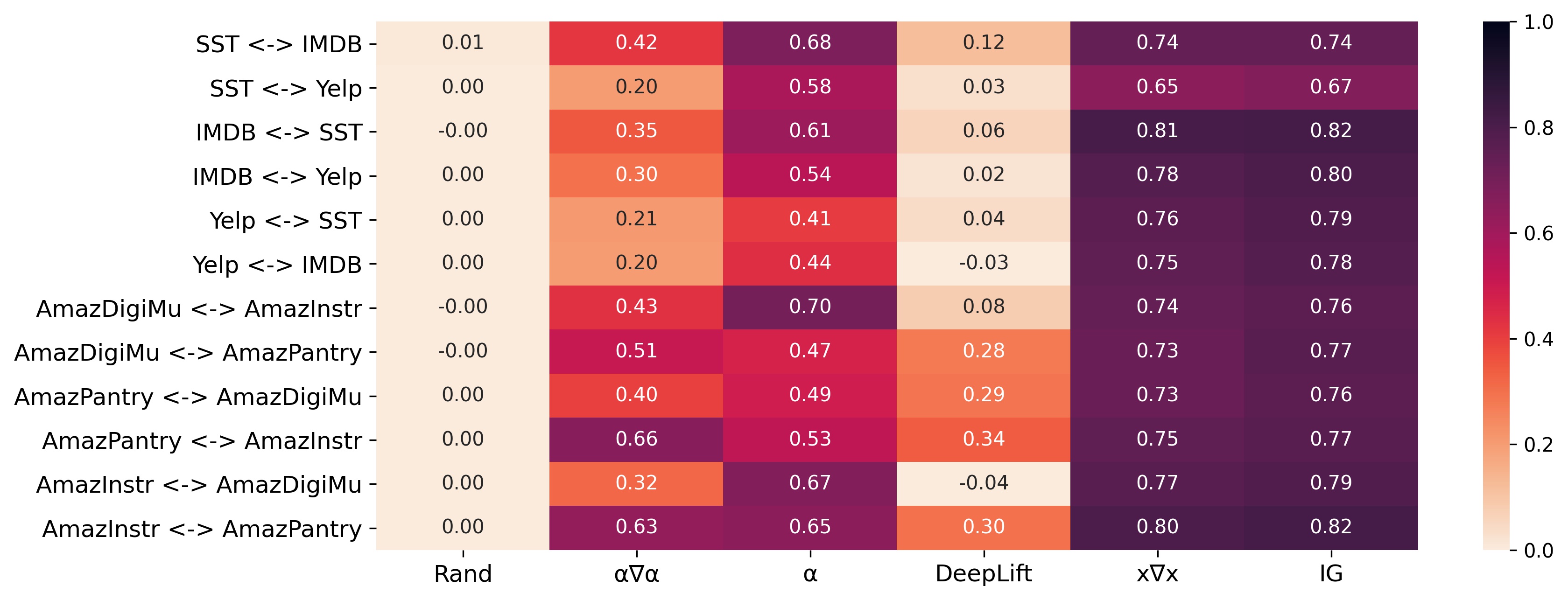
We examine why and IG, do not perform as well as DeepLift and when using FRESH. We therefore conduct a study to gain better understand this. We first fix the domain of the data we evaluate on and then compute the correlation between importance rankings using any single feature attribution from: (1) a model trained on the same domain with the evaluation data and (2) a model from trained on a different distribution (out-of-domain trained model). High correlations suggest that a feature attribution from an out-of-domain trained model, produce similar importance distributions with that of an in-domain model (i.e. both attend to similar tokens to make a prediction). Therefore, we assume that this will lead to high predictive performance out-of-domain. In Figure 2 we show Spearman’s ranking correlation across dataset pairs, between a model trained on the same distribution as the evaluation data (ID) and an out-of-domain trained model (OOD), such that (ID <-> OOD).
As expected, the random baseline produced almost no correlation between models. An interesting observation is that two of the gradient-based methods ( and IG) produce strongly correlated rankings. This suggests that these two metrics produce generalizable rankings irrespective of the domain shift, when comparing to the remainder of the feature attribution approaches. Surprisingly, Deeplift importance rankings exhibit almost low to no correlation betweenen them, despite being also gradient-based. We hypothesize that this happens because DeepLift considers a baseline input to compute its importance distribution, which highly depends on the model and as such is de-facto normalized and perhaps generalizes better.
| ID | OOD | Rand | DeepLift | IG | |||
|---|---|---|---|---|---|---|---|
| SST | IMDB | 0.06 | 0.26 | 0.39 | 0.37 | 0.54 | 0.55 |
| SST | Yelp | 0.07 | 0.11 | 0.27 | 0.29 | 0.46 | 0.49 |
| IMDB | SST | 0.02 | 0.13 | 0.25 | 0.15 | 0.43 | 0.43 |
| IMDB | Yelp | 0.02 | 0.08 | 0.16 | 0.09 | 0.43 | 0.43 |
| Yelp | SST | 0.02 | 0.08 | 0.12 | 0.18 | 0.37 | 0.39 |
| Yelp | IMDB | 0.02 | 0.05 | 0.12 | 0.10 | 0.40 | 0.41 |
| AmazDigiMu | AmazInstr | 0.13 | 0.22 | 0.38 | 0.16 | 0.60 | 0.61 |
| AmazDigiMu | AmazPantry | 0.13 | 0.30 | 0.36 | 0.27 | 0.60 | 0.62 |
| AmazPantry | AmazDigiMu | 0.14 | 0.28 | 0.35 | 0.27 | 0.60 | 0.63 |
| AmazPantry | AmazInstr | 0.14 | 0.39 | 0.42 | 0.21 | 0.62 | 0.64 |
| AmazInstr | AmazDigiMu | 0.08 | 0.16 | 0.29 | 0.12 | 0.54 | 0.57 |
| AmazInstr | AmazPantry | 0.08 | 0.29 | 0.36 | 0.14 | 0.57 | 0.59 |
| ID | OOD | Rand | DeepLift | IG | |||
|---|---|---|---|---|---|---|---|
| SST | IMDB | 0.10 | 0.32 | 0.47 | 0.33 | 0.60 | 0.61 |
| SST | Yelp | 0.11 | 0.19 | 0.35 | 0.25 | 0.54 | 0.56 |
| IMDB | SST | 0.10 | 0.29 | 0.41 | 0.17 | 0.60 | 0.61 |
| IMDB | Yelp | 0.10 | 0.21 | 0.34 | 0.14 | 0.59 | 0.61 |
| Yelp | SST | 0.10 | 0.18 | 0.28 | 0.16 | 0.55 | 0.57 |
| Yelp | IMDB | 0.10 | 0.16 | 0.29 | 0.12 | 0.56 | 0.58 |
| AmazDigiMu | AmazInstr | 0.17 | 0.29 | 0.47 | 0.16 | 0.66 | 0.68 |
| AmazDigiMu | AmazPantry | 0.17 | 0.36 | 0.44 | 0.26 | 0.66 | 0.69 |
| AmazPantry | AmazDigiMu | 0.17 | 0.33 | 0.42 | 0.27 | 0.66 | 0.68 |
| AmazPantry | AmazInstr | 0.17 | 0.46 | 0.49 | 0.24 | 0.67 | 0.69 |
| AmazInstr | AmazDigiMu | 0.13 | 0.24 | 0.43 | 0.11 | 0.64 | 0.66 |
| AmazInstr | AmazPantry | 0.13 | 0.40 | 0.50 | 0.20 | 0.67 | 0.68 |
for out-of-domain detection?:
An interesting case is that of , where we observe moderate to strong correlations across all test-cases. What is more evident, is that in the OOD tuples we considered, it appears that stronger correlations appear where the OOD task and the ID task are closer together. For example in the case of SST and IMDB (both sentiment analysis tasks for movie reviews), produces a strong correlation (0.68). This contrasts the moderate correlation of 0.58 between SST and Yelp, which is for restaurant reviews. This is also evident in the case of AmazDigiMu and AmazInstr, where both tasks are for review classification, but for musical related purchases. They both score strong correlations between them and moderate correlations with reviews for pantry purchases (AmazPantry). This observation might suggest, that using these correlation metrics with might be an indicator of the degree of task-domain-shift. Our observation is also supported by the findings of Adebayo et al. (2020), who show that feature attributions are good indicators of detecting spurious correlation signals in computer vision tasks.Considering we observe a wide range of correlations, ranging from low in the AmazInstr-AmazDigiMu pair to strong in the AmazPantry-AmazInstr pair, which we cannot interpret as something meaningful.
| ID | OOD | Rand | DeepLift | IG | |||
|---|---|---|---|---|---|---|---|
| SST | IMDB | 0.20 | 0.42 | 0.57 | 0.34 | 0.68 | 0.67 |
| SST | Yelp | 0.21 | 0.31 | 0.46 | 0.27 | 0.61 | 0.62 |
| IMDB | SST | 0.20 | 0.39 | 0.52 | 0.26 | 0.69 | 0.69 |
| IMDB | Yelp | 0.20 | 0.32 | 0.46 | 0.22 | 0.67 | 0.68 |
| Yelp | SST | 0.20 | 0.29 | 0.41 | 0.24 | 0.64 | 0.66 |
| Yelp | IMDB | 0.20 | 0.27 | 0.42 | 0.20 | 0.65 | 0.66 |
| AmazDigiMu | AmazInstr | 0.23 | 0.37 | 0.55 | 0.21 | 0.71 | 0.73 |
| AmazDigiMu | AmazPantry | 0.24 | 0.44 | 0.51 | 0.32 | 0.71 | 0.74 |
| AmazPantry | AmazDigiMu | 0.24 | 0.40 | 0.50 | 0.33 | 0.71 | 0.73 |
| AmazPantry | AmazInstr | 0.24 | 0.54 | 0.57 | 0.32 | 0.72 | 0.73 |
| AmazInstr | AmazDigiMu | 0.21 | 0.33 | 0.54 | 0.16 | 0.70 | 0.72 |
| AmazInstr | AmazPantry | 0.21 | 0.51 | 0.60 | 0.30 | 0.72 | 0.74 |
Correlation values and FRESH:
We first observe that the lowest correlated feature attributions and DeepLift perform the better on FRESH, followed by which displays moderate correlations and at the end of the spectrum the two gradient-based methods which display high correlations. Contrary to our initial assumption, this suggests that the attributions which generalize better (i.e. return rationales that result in higher FRESH performance) are those which exhibit low to no correlations.
Agreement at different rationale lengths:
As the correlation analysis considers the entire length of the sequence, we now examine a scenario where we have a priori defined rationale lengths. Similarly to the correlation analysis, we now compute the agreement in tokens between ID feature attribution rankings to those of an OOD trained model. In Tables 14, 15 and 16 we therefore show the token agreement between in-domain and out-of-domain post-hoc explanations (on the same data) for 2%, 10% and 20% rationale lengths.
Our findings show that across all rationale lengths, results largely agree with the correlation analysis. The two gradient-based methods exhibit higher agreement than the remainder, with and DeepLift recording the lowest agreements. Surprisingly, the poorest performers on out-of-domain FRESH record the highest agreement in tokens with in-domain models. Whilst this suggests that they generalize better, we believe that the inhibiting factor to their performance is their limited in-domain capabilities (i.e. they record the lowest in-domain FRESH performance with TopK).
Appendix F Post-hoc Explanation Faithfulness - Extended
In Tables 17, 18 and 19, we present post-hoc explanation sufficiency and comprehensiveness scores at 2%, 10% and 20% rationale lengths.
| Train | Test | Normalized Sufficiency | Normalized Comprehensiveness | ||||||||||
|---|---|---|---|---|---|---|---|---|---|---|---|---|---|
| Rand | DeepLift | IG | Rand | DeepLift | IG | ||||||||
| SST | SST | 0.42 | 0.46 | 0.40 | 0.42 | 0.43 | 0.43 | 0.11 | 0.29 | 0.00 | 0.11 | 0.19 | 0.19 |
| IMDB | 0.35 | 0.40 | 0.33 | 0.35 | 0.34 | 0.35 | 0.11 | 0.39 | 0.14 | 0.13 | 0.17 | 0.18 | |
| Yelp | 0.36 | 0.41 | 0.32 | 0.37 | 0.32 | 0.33 | 0.10 | 0.31 | 0.08 | 0.10 | 0.11 | 0.13 | |
| IMDB | IMDB | 0.36 | 0.42 | 0.39 | 0.37 | 0.37 | 0.37 | 0.05 | 0.27 | 0.14 | 0.06 | 0.11 | 0.12 |
| SST | 0.29 | 0.30 | 0.29 | 0.30 | 0.30 | 0.30 | 0.16 | 0.33 | 0.16 | 0.16 | 0.21 | 0.19 | |
| Yelp | 0.40 | 0.45 | 0.43 | 0.41 | 0.40 | 0.40 | 0.10 | 0.35 | 0.21 | 0.10 | 0.13 | 0.13 | |
| Yelp | Yelp | 0.12 | 0.13 | 0.13 | 0.13 | 0.13 | 0.13 | 0.02 | 0.06 | 0.01 | 0.02 | 0.04 | 0.05 |
| SST | 0.47 | 0.46 | 0.46 | 0.48 | 0.47 | 0.47 | 0.08 | 0.09 | 0.00 | 0.09 | 0.12 | 0.12 | |
| IMDB | 0.11 | 0.11 | 0.11 | 0.12 | 0.11 | 0.11 | 0.07 | 0.19 | 0.10 | 0.08 | 0.10 | 0.10 | |
| AmazDigiMu | AmazDigiMu | 0.24 | 0.42 | 0.16 | 0.17 | 0.30 | 0.29 | 0.09 | 0.25 | 0.04 | 0.02 | 0.12 | 0.13 |
| AmazInstr | 0.17 | 0.33 | 0.13 | 0.13 | 0.21 | 0.21 | 0.14 | 0.41 | 0.10 | 0.06 | 0.17 | 0.18 | |
| AmazPantry | 0.27 | 0.45 | 0.20 | 0.21 | 0.30 | 0.29 | 0.18 | 0.43 | 0.10 | 0.05 | 0.20 | 0.22 | |
| AmazPantry | AmazPantry | 0.23 | 0.34 | 0.27 | 0.16 | 0.23 | 0.22 | 0.11 | 0.32 | 0.19 | 0.03 | 0.15 | 0.15 |
| AmazDigiMu | 0.22 | 0.35 | 0.29 | 0.16 | 0.22 | 0.22 | 0.10 | 0.29 | 0.19 | 0.03 | 0.12 | 0.12 | |
| AmazInstr | 0.14 | 0.23 | 0.18 | 0.11 | 0.15 | 0.14 | 0.12 | 0.39 | 0.23 | 0.07 | 0.16 | 0.17 | |
| AmazInstr | AmazInstr | 0.13 | 0.18 | 0.09 | 0.11 | 0.13 | 0.13 | 0.16 | 0.40 | 0.05 | 0.08 | 0.17 | 0.18 |
| AmazDigiMu | 0.19 | 0.29 | 0.12 | 0.13 | 0.19 | 0.18 | 0.14 | 0.35 | 0.04 | 0.05 | 0.14 | 0.15 | |
| AmazPantry | 0.20 | 0.30 | 0.14 | 0.15 | 0.20 | 0.20 | 0.19 | 0.45 | 0.04 | 0.08 | 0.18 | 0.21 | |
| Train | Test | Normalized Sufficiency | Normalized Comprehensiveness | ||||||||||
|---|---|---|---|---|---|---|---|---|---|---|---|---|---|
| Rand | DeepLift | IG | Rand | DeepLift | IG | ||||||||
| SST | SST | 0.43 | 0.55 | 0.43 | 0.46 | 0.44 | 0.45 | 0.16 | 0.42 | 0.20 | 0.22 | 0.25 | 0.25 |
| IMDB | 0.36 | 0.65 | 0.44 | 0.37 | 0.36 | 0.36 | 0.19 | 0.69 | 0.39 | 0.24 | 0.25 | 0.26 | |
| Yelp | 0.37 | 0.67 | 0.37 | 0.39 | 0.33 | 0.34 | 0.17 | 0.58 | 0.25 | 0.20 | 0.22 | 0.24 | |
| IMDB | IMDB | 0.37 | 0.64 | 0.54 | 0.40 | 0.39 | 0.39 | 0.10 | 0.55 | 0.30 | 0.17 | 0.18 | 0.18 |
| SST | 0.28 | 0.32 | 0.29 | 0.30 | 0.30 | 0.30 | 0.23 | 0.48 | 0.29 | 0.29 | 0.30 | 0.29 | |
| Yelp | 0.41 | 0.54 | 0.46 | 0.43 | 0.41 | 0.41 | 0.18 | 0.58 | 0.36 | 0.22 | 0.24 | 0.24 | |
| Yelp | Yelp | 0.17 | 0.22 | 0.23 | 0.26 | 0.19 | 0.20 | 0.05 | 0.15 | 0.05 | 0.06 | 0.08 | 0.08 |
| SST | 0.48 | 0.49 | 0.47 | 0.50 | 0.46 | 0.46 | 0.13 | 0.23 | 0.15 | 0.16 | 0.20 | 0.20 | |
| IMDB | 0.13 | 0.29 | 0.29 | 0.22 | 0.14 | 0.15 | 0.13 | 0.35 | 0.28 | 0.16 | 0.18 | 0.19 | |
| AmazDigiMu | AmazDigiMu | 0.33 | 0.67 | 0.24 | 0.25 | 0.39 | 0.36 | 0.11 | 0.34 | 0.08 | 0.06 | 0.15 | 0.16 |
| AmazInstr | 0.28 | 0.67 | 0.22 | 0.26 | 0.29 | 0.28 | 0.19 | 0.57 | 0.19 | 0.15 | 0.22 | 0.24 | |
| AmazPantry | 0.33 | 0.64 | 0.25 | 0.28 | 0.36 | 0.34 | 0.22 | 0.55 | 0.17 | 0.12 | 0.25 | 0.26 | |
| AmazPantry | AmazPantry | 0.23 | 0.46 | 0.34 | 0.17 | 0.24 | 0.23 | 0.15 | 0.45 | 0.29 | 0.10 | 0.20 | 0.21 |
| AmazDigiMu | 0.22 | 0.46 | 0.35 | 0.16 | 0.23 | 0.22 | 0.13 | 0.42 | 0.29 | 0.10 | 0.17 | 0.17 | |
| AmazInstr | 0.14 | 0.42 | 0.27 | 0.12 | 0.16 | 0.15 | 0.18 | 0.59 | 0.40 | 0.17 | 0.24 | 0.25 | |
| AmazInstr | AmazInstr | 0.13 | 0.28 | 0.09 | 0.12 | 0.13 | 0.13 | 0.23 | 0.58 | 0.16 | 0.22 | 0.24 | 0.25 |
| AmazDigiMu | 0.19 | 0.32 | 0.12 | 0.14 | 0.20 | 0.18 | 0.18 | 0.47 | 0.10 | 0.14 | 0.20 | 0.20 | |
| AmazPantry | 0.21 | 0.35 | 0.15 | 0.17 | 0.21 | 0.21 | 0.24 | 0.57 | 0.12 | 0.18 | 0.24 | 0.27 | |
| Train | Test | Normalized Sufficiency | Normalized Comprehensiveness | ||||||||||
|---|---|---|---|---|---|---|---|---|---|---|---|---|---|
| Rand | DeepLift | IG | Rand | DeepLift | IG | ||||||||
| SST | SST | 0.45 | 0.68 | 0.51 | 0.51 | 0.48 | 0.49 | 0.22 | 0.54 | 0.34 | 0.33 | 0.32 | 0.34 |
| IMDB | 0.38 | 0.77 | 0.55 | 0.39 | 0.37 | 0.38 | 0.29 | 0.80 | 0.54 | 0.36 | 0.34 | 0.36 | |
| Yelp | 0.39 | 0.83 | 0.57 | 0.41 | 0.37 | 0.38 | 0.25 | 0.71 | 0.44 | 0.30 | 0.32 | 0.34 | |
| IMDB | IMDB | 0.37 | 0.75 | 0.62 | 0.42 | 0.41 | 0.42 | 0.16 | 0.73 | 0.47 | 0.30 | 0.27 | 0.27 |
| SST | 0.26 | 0.40 | 0.31 | 0.31 | 0.31 | 0.30 | 0.32 | 0.65 | 0.42 | 0.41 | 0.42 | 0.42 | |
| Yelp | 0.42 | 0.62 | 0.50 | 0.43 | 0.44 | 0.44 | 0.28 | 0.67 | 0.47 | 0.35 | 0.36 | 0.37 | |
| Yelp | Yelp | 0.25 | 0.43 | 0.41 | 0.40 | 0.28 | 0.30 | 0.09 | 0.25 | 0.12 | 0.13 | 0.14 | 0.15 |
| SST | 0.49 | 0.55 | 0.51 | 0.53 | 0.48 | 0.48 | 0.20 | 0.35 | 0.27 | 0.26 | 0.28 | 0.29 | |
| IMDB | 0.19 | 0.53 | 0.50 | 0.34 | 0.24 | 0.25 | 0.20 | 0.46 | 0.40 | 0.27 | 0.28 | 0.28 | |
| AmazDigiMu | AmazDigiMu | 0.43 | 0.81 | 0.47 | 0.35 | 0.52 | 0.50 | 0.14 | 0.41 | 0.17 | 0.10 | 0.19 | 0.20 |
| AmazInstr | 0.37 | 0.79 | 0.49 | 0.42 | 0.43 | 0.42 | 0.24 | 0.63 | 0.33 | 0.23 | 0.28 | 0.30 | |
| AmazPantry | 0.42 | 0.76 | 0.45 | 0.37 | 0.47 | 0.45 | 0.26 | 0.61 | 0.31 | 0.20 | 0.30 | 0.32 | |
| AmazPantry | AmazPantry | 0.27 | 0.63 | 0.46 | 0.19 | 0.30 | 0.29 | 0.21 | 0.57 | 0.40 | 0.17 | 0.28 | 0.29 |
| AmazDigiMu | 0.25 | 0.63 | 0.46 | 0.18 | 0.28 | 0.27 | 0.19 | 0.55 | 0.39 | 0.16 | 0.25 | 0.25 | |
| AmazInstr | 0.16 | 0.61 | 0.42 | 0.14 | 0.21 | 0.20 | 0.27 | 0.72 | 0.54 | 0.26 | 0.35 | 0.36 | |
| AmazInstr | AmazInstr | 0.15 | 0.46 | 0.15 | 0.18 | 0.17 | 0.16 | 0.31 | 0.72 | 0.33 | 0.34 | 0.32 | 0.34 |
| AmazDigiMu | 0.21 | 0.46 | 0.16 | 0.17 | 0.23 | 0.20 | 0.24 | 0.60 | 0.22 | 0.22 | 0.26 | 0.27 | |
| AmazPantry | 0.23 | 0.49 | 0.18 | 0.21 | 0.24 | 0.23 | 0.31 | 0.68 | 0.28 | 0.28 | 0.32 | 0.35 | |