(a) initialization

(b) intermediate result

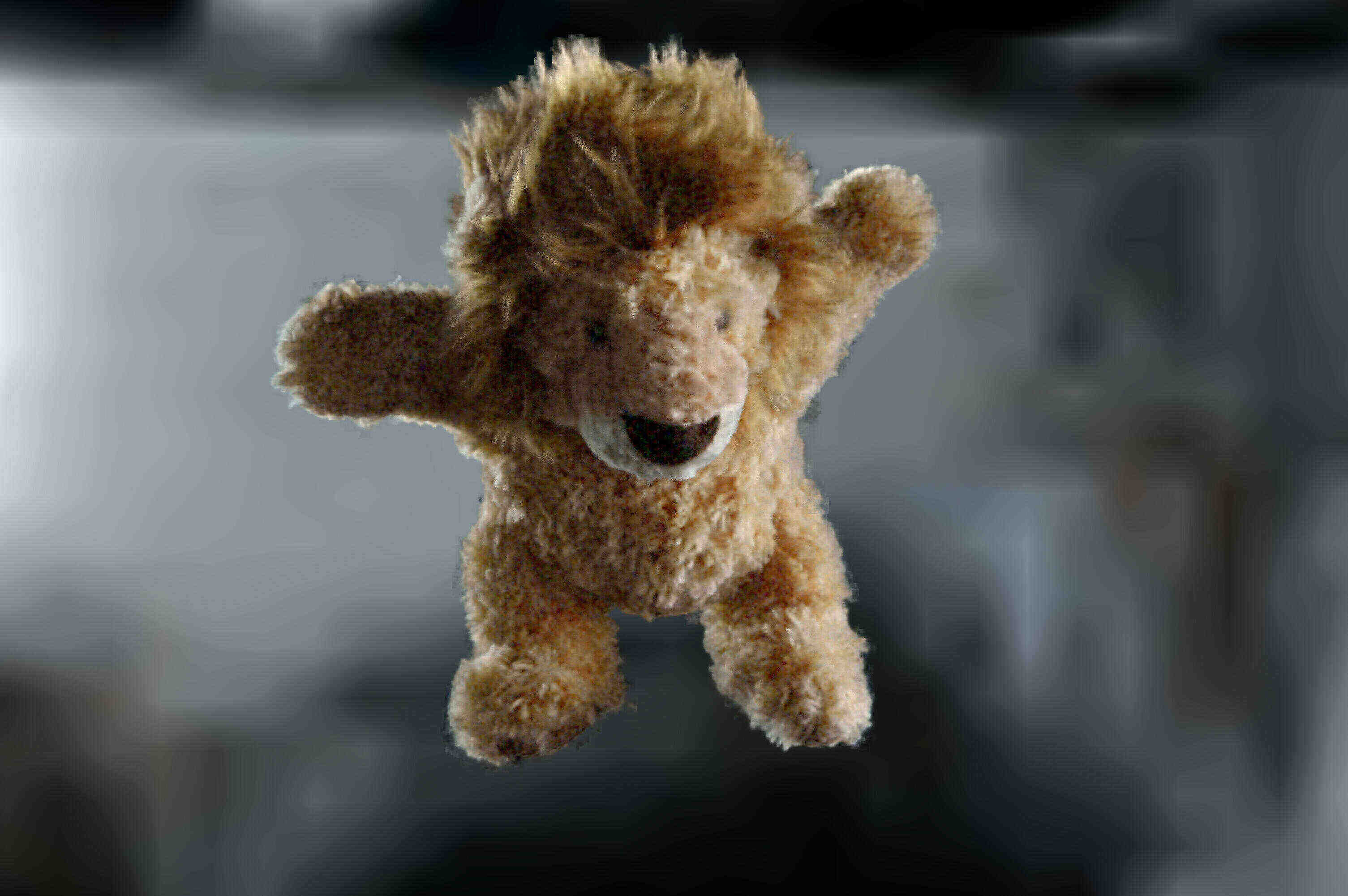
(c) final result

(d) ground truth

Figure 1. Our from-scratch reconstruction of a plush lion demonstrated by three renderings (left) which gradually match an hold-out test photo (right).

ERF: Explicit Radiance Field Reconstruction From Scratch

Abstract.

We propose a novel explicit dense 3D reconstruction approach that processes a set of images of a scene with sensor poses and calibrations and estimates a photo-real digital model. One of the key innovations is that the underlying volumetric representation is completely explicit in contrast to neural network-based (implicit) alternatives. We encode scenes explicitly using clear and understandable mappings of optimization variables to scene geometry and their outgoing surface radiance. We represent them using hierarchical volumetric fields stored in a sparse voxel octree. Robustly reconstructing such a volumetric scene model with millions of unknown variables from registered scene images only is a highly non-convex and complex optimization problem. To this end, we employ stochastic gradient descent (Adam) which is steered by an inverse differentiable renderer.

We demonstrate that our method can reconstruct models of high quality that are comparable to state-of-the-art implicit methods. Importantly, we do not use a sequential reconstruction pipeline where individual steps suffer from incomplete or unreliable information from previous stages, but start our optimizations from uniformed initial solutions with scene geometry and radiance that is far off from the ground truth. We show that our method is general and practical. It does not require a highly controlled lab setup for capturing, but allows for reconstructing scenes with a vast variety of objects, including challenging ones, such as outdoor plants or furry toys. Finally, our reconstructed scene models are versatile thanks to their explicit design. They can be edited interactively which is computationally too costly for implicit alternatives.

1. Introduction

The vast field of 3D reconstruction has been researched actively for decades. Diverse pioneering works were already published in the 1990s (Hoppe et al., 1992; Turk and Levoy, 1994; Curless and Levoy, 1996; Gortler et al., 1996; Szeliski and Golland, 1999; Seitz and Dyer, 1999). Yet, there has recently been a strong increase in interest in the field due to the availability of powerful optimization techniques such as Adam (Kingma and Ba, 2014) combined with novel neural-network-based extensions of such traditional earlier works (Lombardi et al., 2019; Mildenhall et al., 2019, 2020; Yariv et al., 2020; Zhou et al., 2018). We also employ powerful optimization techniques, but in contrast to the current research trend, which creates the impression that state-of-the-art reconstructions are only possible using neural-network-based models, we reconstruct explicit high-quality 3D models from scratch; i.e., only from multi-view images (with sensor poses and calibrations). In the course of this, we employ inverse differentiable rendering paired with Adam as a variant of and without any implicit components based on neural networks. That way, we can provide a practical reconstruction method for editable models. Specifically, it allows for capturing of static scenes by simply taking photos from different view points.

In contrast, the recently popular works NeRF (Mildenhall et al., 2020) and IDR (Yariv et al., 2020) as well as their many follow-up works employ implicit scene representations (often MLPs). These network-based methods are able to generate novel views with extremely high fidelity, while only requiring very compact implicit scene models. However, the fact that the internals of these implicit models cannot be interpreted poses significant challenges and leveraging the success of traditional graphics and vision techniques by combining them with implicit models is an open and challenging research question. Scaling purely implicit models for large scale scenes is also challenging. It is unclear how to properly increase the capacity of purely implicit models, i.e., how to extend the black box internals, in a controlled manner without overfitting or oversmoothing artifacts. Avoiding these limitations motivated recent hybrid extensions as mixes of im- and explicit models (Hedman et al., 2021; Liu et al., 2020; Martel et al., 2021; Reiser et al., 2021; Yu et al., 2021). Additionally, implicit models come at the cost of reduced versatility. In particular, they are less suited for 3D content authoring, e.g., using interactive tools like Blender. Editing operations on implicitly defined model parts first have to go through a black box compression layer inherent to their implicit definition which entails costly optimization. Although, some early works focus on editing of implicit models (Liu et al., 2021; Yang et al., 2021), they are rather a proof of concept targeting small scale synthetic objects and are too costly for practical use.

The goal of this work is to address these shortcomings. We designed an explicit approach with the benefits of being interpretable, scalable and editable. Our method can handle complex scenes with tiny intricate scene details, e.g., the fur of the plush lion in Fig. 1. We further demonstrate that our reconstructed models are suitable for post processing, such as interactive editing via tools like Blender, and that they are comparable to state-of-the-art implicit models regarding photo consistency.

Our contributions are the following:

1. a hierarchical, multi-resolution, sparse grid data structure using SVOs with 3D fields for opacity and outgoing radiance surface light fields (SLFs) to explicitly represent scene geometry and appearance,

2. a storage and interpolation scheme using local planes to efficiently represent 3D fields with little voxel artifacts,

3. a simple, yet effective background model for distant scene radiance to handle unbounded scene volumes,

4. an opacity compositing rendering algorithm that takes pixel footprints into account and thus avoids level of detail (LoD) aliasing,

5. a uniform, hierarchical (coarse-to-fine) optimization scheme to make the approach feasible and scalable,

6. a practical reconstruction method for freely captured multi-view images of static scenes, neither requiring object masks, nor a sophisticated model initialization.

Our novel scene representation has several benefits. We represent scenes using complex (high-dimensional), continuous, volumetric and differentiable 3D fields suitable for intricate geometry details that leverage powerful optimization methods such as Adam (Kingma and Ba, 2014). Unlike ours, previous explicit and discrete representations, such as multi-sphere images (MSIs) or general meshes, make strong assumptions or are inherently difficult to optimize due to their challenging objective function originating from their discrete model design. Compared to network-based alternatives, while using more memory, our novel scene representation is explicit and better suited for interactive editing as transformation operations do not go through an additional compression layer inherent to implicit model definitions. Further, we argue that our explicit models facilitate research to leverage the strengths of traditional graphics techniques. E.g., our spatial scene partitioning can directly accelerate ray-based queries of scenes, which are fundamental to implement complex shading, instead of directly storing SLFs. We demonstrate a versatile and practical explicit approach that neither requires a restrictive laboratory setup ((Bi et al., 2020b, a)), nor does it need object masks ((Yariv et al., 2020; Boss et al., 2021; Zhang et al., 2021a)) which tend to be difficult to acquire or might be inaccurate (hard or impossible for intricate geometry like the fur in Fig. 1). Finally, our 4D scene partitioning (3D space plus LoD) is uniform and straightforward to apply to captured scenes. It neither requires an artificial LoD separation ((Mildenhall et al., 2020; Barron et al., 2021)), nor does it require a special scene-dependent parameterization ((Mildenhall et al., 2020; Zhang et al., 2020)).

2. Related Work

In the following, we provide a short overview of closely related works, whereas we focus on the im- or explicity of the underlying scene representations and the corresponding practicality or usability implications. First, we discuss a group of methods that model scenes using single-hypothesis surfaces. Representations from this group tend to be challenging during optimization or they make strong assumptions limiting their use. Second, we look at methods trying to circumvent the latter disadvantages. The second group models scenes using soft-relaxed surfaces. I.e., these methods employ volumetric representations that support multiple simultaneous hypotheses for the same surface. Our approach falls into the second group. We provide a soft-relaxed, but very explicit representation. Our focus is on comprehensibility and versatility of the underlying representation thanks to its explicit design.

2.1. Models with single surface hypothesis

First, we review representations with ”strict” surfaces (without geometry soft relaxation).

Layered meshes

Layered meshes are special cases designed for novel view synthesis only. That is why they can be implemented using very regular and simple geometric structures. I.e., they model a complete scene using only a pyramid of rectangles (MPI) or via concentric spheres (MSI). Due to their strong focus and simplicity, they allow for efficient and high-quality novel view rendering at the same time. One of the first such methods reconstructs a scene as explicit MPI with regular depths and plane texels directly consisting of opacity and color values that are rendered using opacity compositing (Szeliski and Golland, 1999). More recent works are rather hybrid methods with learned neural networks that predict explicit RGBA layers for MPIs (Zhou et al., 2018) or MSIs (Broxton et al., 2020), respectively assuming a novel viewer in front of the rectangle pyramid or at the center of the concentric spheres. Even more on the implicit end, (Wizadwongsa et al., 2021) predict hybrid mesh layers with neural basis functions for the appearance of scene surfaces, since they better model view-dependent effects than simple RGBA texels. Such learned layered models interpolate the captured radiance fields of individual scenes well within a limited range of views. However, they fail to synthesize farther away views and the reconstructed geometry can deviate significantly from the actual surfaces. To maintain the quality, faking view-dependent effects via ”ghost” layers is required, which prevents manual scene editing.

General, directly optimized meshes

In contrast to MPIs and MSIs, general mesh-based methods aim at obtaining a complete and accurate surface reconstruction. Therefore the results are much more versatile, but also more difficult to reconstruct. Direct full mesh optimization (Aroudj et al., 2017; Luan et al., 2021) is difficult, because the discrete representation leads to highly non-convex objective functions. In particular, such approaches are prone to miss necessary gradients during optimization and they require an initialization that is already close to the global optimum. They can quickly degrade to invalid manifolds and often cannot improve the topology during optimization.

Continuously and implicitly defined surfaces

Owing to the drawbacks of directly optimized meshes, the community also researched continuous representations that implicitly define scene surfaces and entail a better behaviour of the objective function. For example, the surfaces extracted from the SDF representations (Yariv et al., 2020; Zhang et al., 2021a; Kellnhofer et al., 2021) are manifolds by definition and can easily adapt topology during optimization. However, these methods still assume that the scene can be well reconstructed using clearly defined single-hypothesis surfaces. Depending on where the implicitly defined surface intersects or does not intersect view rays, this leads to discontinuities in the objective function that are hard to handle. To avoid the local optima originating from these discontinuities, additional constraints from object segmentation masks are required. Since these masks by themselves are hard or impossible to obtain without human assistance, this poses a significant limitation. VolSDF is a follow up work which circumvents this limitation. In particular, the authors again suggest modeling scene surfaces using SDFs. However, the key difference is that, to account for surface uncertainty and enforce geometric constraints (Eikonal loss) at the same time, they infer scene density fields from the underlying SDFs. Then they can render the density fields using volume rendering which facilitates optimization and removes the need for masks. Note that, thanks to its density-based uncertainty, VolSDF is a hybrid that belongs to both related work groups discussed here. Disadvantageously, a single, scene-global parameter controls surface uncertainty which makes it less suited for varying fine and intricate geometry. Also only results for small scale scenes were shown by the authors. In general, intricate geometry of for example plants or fur as in Fig. 1 is difficult to represent using SDF- and mesh-based methods. Representing such geometry accurately often requires a resolution with prohibitively high costs. The limitations of methods with single-hypothesis surfaces motivated not only VolSDF, but also other recent, continuous representations. As the next subsection explains, these approaches represent geometry using volumetric fields that inherently support multiple surface estimates at the same time to facilitate optimization and also support fine and intricate geometry approximations.

2.2. Models with multiple surface hypotheses

This subsection reviews methods that model scenes with soft-relaxed geometry. We begin with models that are on the very implicit end and continue going towards the very explicit end of scene representations.

NeRFs with baked-in SLFs

Thanks to the pioneering implicit approach NeRF (Mildenhall et al., 2020), MLPs that encode the geometry and surface radiance (SLF) of individual scenes volumetrically have become the recently dominant representation. They model individual scenes via 5D fields consisting of continuous volumetric density for geometry coupled with view-dependent surface radiance for appearance. These compact MLP models represent surfaces continuously and in a soft-relaxed and statistical manner. Meaning they consist of continuous fields that smoothly change during optimization. They furthermore implement a soft relaxation by allowing to model opaque surfaces as spread out or partially transparent. The latter allows for multiple surface hypotheses during optimization which improves convergence by reducing the issue of missing correct gradients. To avoid novel view synthesis errors, they can furthermore approximate fine and intricate surfaces statistically. Nevertheless, the original NeRF method came with severe limitations owing to, for example, its special scene parameterization, capture setup requirements or its static scene radiance assumption. I.e., aliasing issues and multi-scale input data are focused by (Barron et al., 2021), the follow-up work (Zhang et al., 2020) allows for a more flexible capture setup or (Martin-Brualla et al., 2021) targeted the static radiance assumption by disentangling transient occluders from the static parts of a scene and by additional latent codes for per-image variations.

Decomposed NeRFs with physically-based components

Other follow-up works, such as (Bi et al., 2020b; Boss et al., 2021; Srinivasan et al., 2021; Zhang et al., 2021b) focus on more explicit models by decomposing the previously directly stored scene radiance into more explicit components. By jointly estimating incoming illumination as well as surface geometry and materials, they aim at re-achieving some of the versatility of traditional explicit representations. However, these approaches either require a very restrictive laboratory capture setup, object masks or they only work for small scale scenes with centered objects. Note that object masks also implicitly prevent intricate materials, e.g., fur or grass, for which it is difficult to acquire accurate masks in practice. Furthermore, in the case of NeRV (Srinivasan et al., 2021)), only results for limited synthetic data instead of captured real-world scenes are presented. Like the original NeRF, our scene models also directly store the outgoing surface radiance of individual static radiance scenes. However, we store the outgoing radiance using a sparse hierarchical grid with SHs instead of a black box MLP. We leave decomposing the convolution of incoming light with surface materials as an extension for further research. Given our simplifying design choice for directly storing and optimizing static SLFs, our models allow for direct geometry editing and simple transformations of the surface appearance, as we will demonstrate later. Physically-based editing of surface materials or scene light transport is also left for future work at this time.

The earlier mentioned decomposition approach (Bi et al., 2020b) is an exception regarding two aspects. First, it does not employ MLPs, but a 3D convolutional neural network (CNN) that decodes surface geometry and materials into an explicit and dense voxel grid. Second, similar to our work, the authors suggest to implement volume rendering using traditional opacity compositing. Compared to our approach, their method is however limited to a small scale laboratory capture setup with black background. It furthermore requires a single point light that coincides with the capturing sensor. Finally, it is strongly limited by its simple dense grid scene structure and naive scene sampling. In contrast, while our scene models only have baked-in appearance, we are able to optimize for more general scenes with less controlled and unknown static radiance fields. To support highly detailed reconstructions, we present our coarse-to-fine optimization using sparse hierarchical grids with our comparatively more efficient importance sampling scheme.

Spatially explicit hybrids

The hybrid Neural Volumes (Lombardi et al., 2019) represents scenes captured with a light stage using an encoder and decoder network. It decodes a latent code into a regular RGBA voxel grid that is rendered using ray marching and alpha blending. To allow for detailed reconstructions despite the dense regular grids, the authors suggest to also learn warp fields to unfold compressed learned models. However, ray marching through dense grids is still inefficient and RGBA grids cannot handle view-dependent effects without ghost geometry. More recent and more efficient hybrids with implicit and explicit model parts (Liu et al., 2020; Hedman et al., 2021; Reiser et al., 2021) also explicitly partition the 3D scene space into cells, but using more efficient and view-dependent sparse voxel grids. This allows for overall higher model resolution, more efficient scene sampling or faster rendering. These methods respectively cache computationally expensive volume rendering samples, use a single feature-conditioned MLP or many simple and thus low-cost MLPs distributed over the sparsely allocated grid cells. On the contrary, we employ completely explicit scene models. For multi-resolution rendering, efficient sampling and to limit memory consumption, our models built on sparse hierarchical grids. To keep our approach practical and allow for optimizing freely captured and thus uncontrolled scenes, we also directly cache the SLF of scene surfaces using SHs.

SVO hybrids using SH-based appearance

The recently published PlenOctree models (Yu et al., 2021) are also more explicit models and most similar to our scene representations. The authors likewise model individual scenes with static radiance with continuous fields for geometry and appearance that are stored in SVOs. Similar to us, they handle view-dependent effects using SHs. However, in contrast to our method, their method requires a multi-step reconstruction pipeline starting from registered images. The first step of this pipeline is to obtain a coarse NeRF scene model. The NeRF model then defines the space partitioning (and sparsity) of their SVO via its density field. The authors suggest converting the NeRF scene model into the new SVO by dense sampling and finally optimize its per-node geometry and appearance parameters to obtain an improved model. Having the initial coarse NeRF model as free space constraint, reduces memory consumption and helps avoid false clutter in free space.

In contrast, we show that it is feasible to reconstruct 3D scenes directly and uniformly from images with sensor poses and calibrations using an explicit representation. We achieve high model resolution using SVOs that we gradually build and which we optimize with Adam, but without any implicit, network-based model parts. Since in our case free space and surfaces are initially completely unknown, our coarse-to-fine optimization with dynamic voxel allocations is critical to not run out of memory. As important part of the coarse-to-fine optimization, we present our local plane-based storage and interpolation schemes for the volumetric fields attached to our SVOs. These schemes allow for approximating thin and fine geometric details, even initially, when only a coarse SVO is available. The explicit coarse-to-fine reconstruction from registered images furthermore requires efficient scene sampling. We implemented an importance sampling scheme that filters sampling points gradually and according to the current geometry estimate. In that way, our method is not limited by the restrictions coming from an initialization and the SVO structure can dynamically adapt to the scene content without external guide. To avoid blurry transitions from free to occupied space and to obtain clear surface boundaries, our volume rendering also differs by implementing traditional opacity compositing instead of an exponential transmittance model. Note that we model geometry not using a density field, but via an opacity field representing soft-relaxed surfaces only and not occupied space. Our geometry representation is well suited for inverse differentiable rendering, opaque surfaces as well as intricate geometry such as fur. Finally, we use our SVO structure for LoD interpolation and provide a background model for more flexibility regarding capture setups. In contrast to the PlenOctree work, we can also reconstruct scenes with an unbounded volume, e.g., an outdoor scene with all sensor poses roughly facing the same direction.

3. Overview

In the following, we present our scene representation and the corresponding reconstruction algorithm.

3.1. Input and output

We reconstruct explicit 3D models from unordered multi-view input images. In particular, given an unstructured set of images, we first run standard SfM techniques in a preprocess. I.e., we first run COLMAP for sensor poses and intrinsics as well as a sparse feature point cloud. Second, to bound the scene parts of interest to be reconstructed, we manually estimate conservative min- and maximum corners of the scene axis-aligned bounding box (AABB) using the SfM feature points. Third, we run our actual reconstruction algorithm with input data consisting of

1. the multi-view images,

2. their sensor poses and calibrations and

3. the coarse, conservative AABB.

Our reconstruction algorithm outputs a scene model containing an SVO within the given scene AABB. The output scene model further consists of a background model, an environment map that complements the SVO. It represents distant scene regions such as sky for example. Fig. 2 sketches our scene representation.

Figure 2. Scene model sketch. The background model (cube map, left) complements the SVO. The SVO stores detailed surfaces in its leaves (center) and coarser approximations in its inner nodes (right). Each node has an opacity and multiple SH parameters.

The SVO stores the ”actual” scene. First, it stores a volumetric scalar field with opacity defining surface geometry. Second, it stores a volumetric vector field with SHs defining the scene SLF. Note that the opacity models soft-relaxed surfaces and not occupied space. The scene SLF contains the total outgoing radiance for each surface point along each hemispherical direction. Also note that each tree level represents the scene at a specific LoD. I.e., to support varying scene detail level, our SVO represents the scene also using inner nodes analogously to mipmap textures.

Use and limitations

Our scene models are explicit, differentiable and statistical representations. To facilitate robust reconstruction from scratch and editing, the volumetric SVO fields for opacity and outgoing radiance statistically approximate surfaces, allow for multiple surface hypothesis during optimization contrary to ”accurate” surface models and have a clear meaning in contrast to network weights. The model parameters only go through straightforward constraints ensuring physically meaningful values while an solver can still freely update the parameters. Data transformations are simpler for explicit scene models since the operations do not need to go through an additional compression layer inherent to compact network-based models. In case of networks, these operations again require costly optimizations when they target implicitly defined model parts. Equally, initializing our model with a specific state is simpler. In this work, we started reconstructions from scratch with a mostly transparent and uninformed random fog to demonstrate the flexibility and robustness of our approach, see Fig. 1. Though, initializing models using results from prior steps such as SfM would also be straightforward. Physically based scene transformations, e.g., recalculating shadows when the opacity field changes, are however out of scope of this work. We made the simplifying decision to directly store and optimize the radiance outgoing from the scene surfaces using SHs.

3.2. Algorithm overview.

Please see Tab. 1 for the notation we will use throughout the rest of the document. Alg. 1 describes our method on a high level and details will follow in the remaining method sections. Our algorithm first coarsely initializes the new scene model and then gradually extends the SVO (outer loop) according to the repeated optimization of its fields (inner loop).

$\mathbf{L}_{o}$	SVO SLF	$o$	SVO opacity field
$\mathbf{L}_{\infty}$	distant radiance	$\widehat{o}$	unconstrained $o$
$\mathbf{n}(\mathbf{x})$	surf. normal at $\mathbf{x}$	$\mathcal{C}$	loss cache
$\left\{\mathbf{p}_{i}\right\}$	pixel batch; pixel $i$	$\mathbf{r}_{i}$	ray of pixel $p_{i}$
$\mathbf{x}_{c,i}$	sensor center of $\mathbf{r}_{i}$	$\mathbf{d}_{i}$	direction of $\mathbf{r}_{i}$
$o(t_{i,k})$	opacity at $\mathbf{r}_{i}(t_{i,k})$	$\left\{t_{i,j}\right\}$	ray batch depths
$o_{p}(\mathbf{p}_{i})$	pixel opacity $i$	$\left\{t_{i,k}\right\}$	depths subset
$\mathbf{L}_{o}\left(t_{i,l},-\mathbf{d}_{i}\right)$	SLF at $\left(t_{i,l},-\mathbf{d}_{i}\right)$	$\left\{t_{i,l}\right\}$	subset of subset
$\mathbf{L}_{p}(\mathbf{p}_{i})$	pixel radiance $i$	$\mathcal{I}_{p}(\mathbf{p}_{i})$	rendered pixel $i$
$l_{p}(\mathbf{p}_{i})$	photo loss $i$	$\mathcal{I}_{p}^{\text{gt}}(\mathbf{p}_{i})$	ground truth $i$
$\sigma(p_{i})$	pixel footprint i	$Y_{l,m}$	SH basis function
$\rho$	density	$\mathbf{c}_{l,m}$	SH coefficient

Table 1. Notation overview, see Alg. 1 for use. We abbreviate the notation of sampling points on rays when used within our equations. E.g., we denote the opacity of the $j$-th sampling point on the ray $\mathbf{r}_{i}$ at ray depth $t_{i,j}$ which is located at the 3D location $\mathbf{x}=\mathbf{r}_{i}(t_{i,j})$ by $o(t_{i,j})$. An indexed exemplar element $p_{i}$ surrounded by curly brackets denotes a set. E.g., $\left\{\mathbf{p}_{i}\right\}$ is a pixel batch and the renderer samples each view ray $\mathbf{r}_{i}$ for each optimization batch pixel $p_{i}$ at depths $\left\{t_{i,j}\right\}$.

1

// init model & pixel errors cache

SVO = createDenseGrid(AABB) // random $o$, $\mathbf{L}_{o}$

2 $\mathbf{L}_{\infty}$ = randomEnvMapRadiance()

3 $\mathcal{C}$ = highLossForAllInputPixels()

4

// Optimize: inv. diff. rendering &

5 for $n=0$ to $N$ do

6      

      $\left\{\mathbf{p}_{i}\right\}$ = importanceSample($\mathcal{C}$) // error driven

7      

8      $\left\{\mathbf{r}_{i}\left(t\right)=\mathbf{x}_{c,i}+t\cdot\mathbf{d}_{i}\right\}$ = castRays($\left\{\mathbf{p}_{i}\right\}$)

9      

10      $\left\{t_{i,j}\right\}$ = stratifiedSampling(SVO, $\left\{\mathbf{r}_{i}\left(t\right)\right\}$)

       $\left\{t_{i,k}\right\}$ = selectRandomly($\left\{t_{i,j}\right\}$) // uniform

11      

12      $\left\{o(t_{i,k})\right\}$ = getOpacity(SVO, $\left\{t_{i,k}\right\}$)

13      

14      $\left\{t_{i,l}\right\},\left\{o(t_{i,l})\right\}$ = selectRandomly($\left\{t_{i,k}\right\},\left\{o(t_{i,k})\right\}$)

15      

16      $\left\{\mathbf{L}_{o}\left(t_{i,l},-\mathbf{d}_{i}\right)\right\}$ = getSLF(SVO, $\left\{\mathbf{r}_{i}\left(t\right)\right\},\left\{t_{i,l}\right\}$)

17      

18      $\left\{\mathbf{L}_{p}(\mathbf{p}_{i})\right\},\left\{o_{p}(\mathbf{p}_{i})\right\}$ = blend($\left\{o(t_{i,l})\right\}$,$\left\{\mathbf{L}_{o}\left(t_{i,l},-\mathbf{d}_{i}\right)\right\}$)

19       $\left\{\mathbf{L}_{p}(\mathbf{p}_{i})\right\}$ = blend($\left\{\mathbf{L}_{p}(\mathbf{p}_{i})\right\}$,$\left\{o_{p}(\mathbf{p}_{i})\right\}$,$\left\{\mathbf{L}_{\infty}(-\mathbf{d}_{i})\right\}$)

20      

21      $\left\{\mathcal{I}_{p}(\mathbf{p}_{i})\right\}$ = sensorResponses($\left\{\mathbf{L}_{p}(\mathbf{p}_{i})\right\}$)

22      

23      $\left\{l_{p}(\mathbf{p}_{i})\right\}$ = loss($\left\{\mathcal{I}_{p}(\mathbf{p}_{i})\right\}$, $\left\{\mathcal{I}_{p}^{\text{gt}}(\mathbf{p}_{i})\right\}$)

24       SVO, $\mathbf{L}_{\infty}$ = makeStep(SVO, $\mathbf{L}_{\infty}$, $\nabla(\left\{l_{p}(\mathbf{p}_{i})\right\})$)

25      

      $\mathcal{C}$ = update($\mathcal{C}$, $\left\{l_{p}(\mathbf{p}_{i})\right\}$) // track errors

26      

27 end for

28

// New SVO via opacity $o$ and footprints $\sigma$

mergeLeaves(SVO)

  // compact free space

29 if subdivideLeaves(SVO, $\left\{\sigma(p_{i})\right\}$) then

       resetOptimizer()

        // due to new unknowns

30       go to line 1

31      

32 end if

Algorithm 1 Hierarchical optimization

First, our algorithm creates a coarse dense grid, i.e., a full and shallow SVO, within the given scene bounding box. We randomly initialize the 3D fields of the SVO with grayish fog and random radiance (line 1). We similarly randomly initialize the environment map (line 1), as shown in Fig. 1(a).

We then mainly optimize the parameters of the 3D fields without changing the tree structure using multi-view volumetric inverse differentiable rendering (IDR) and (lines 1 - 1). To this end, we randomly select small batches of input image pixels using importance sampling (line 1); cast a ray for each selected pixel into the scene (line 1); distribute scene sampling points along each ray using stratified importance sampling (line 1); query the scene SVO for opacity and SLF samples at these ray sampling points (lines 1, 1); accumulate the returned field samples along each ray and also add the visible background radiance using classical opacity compositing to estimate the totally received scene radiance for each selected pixel (lines 1 - 1); map the received radiance to pixel intensities using the response curve of the sensor (line 1) and, finally, compare the estimated against the input image pixel intensity (line 1) for a model update step (line 1).

Using the gradients of our differentiable volumetric rendering, we iteratively update the scene model using to fit the scene model parameters to the input images for a fixed model resolution (constant model parameter count). Additionally, we infrequently update the tree structure. In particular, we merge or subdivide tree nodes to adapt the resolution based on the current surface geometry estimate. We do so until the SVO is sufficiently detailed with respect to the input images. The following subsections describe these algorithmic steps in more detail.

4. Explicit, sparse, hierarchical model

Our explicit scene model consists of a sparse hierarchical grid, i.e., an SVO. It stores an opacity and RGB SH parameters per node to encode scene surfaces and the radiance leaving them as a scalar and a vector field. The SVO stores both of these fields defined next at each tree level and not only using the leaf nodes to support multiple levels of detail for rendering and optimization. We assume that everything outside of the AABB that bounds the scene SVO is infinitely far away and therefore represent all remaining scene parts using an environment map implemented as a cube map.

4.1. Surface geometry

Our SVO provides a continuous multi-resolution scalar field $o$. To implement it, the SVO stores a continuous, scalar, volumetric field $o:^{3}\mapsto[0,1]$ per tree level. Each tree level with its individual field represents a single LoD. To this end, each tree node, including inner ones, stores 1 floating-point opacity parameter (besides the SLF parameters). Note that inner nodes hence approximate surfaces at a larger scale. The continous opacity field $o$ represents surfaces statistically. Specifically, the opacity $o(\mathbf{x})$ represents the coverage of a planar slice perpendicular to the radiance traveling through $\mathbf{x}$ and thus what percentage of it gets locally absorbed. I.e., it is a surface property expressing what relative percentage of photons statistically hits the surface at $\mathbf{x}$, e.g., $o(\mathbf{x}_{\text{free}})=0$ and $o(\mathbf{x}_{\text{wall}})=1$. As detailed later, the SVO not only interpolates within 3D space, but also blends between the individual LoD fields to serve scale-extended position queries. Only regarding a single LoD and given a query location $\mathbf{x}$, the SVO interpolates the parameters of the tree nodes surrounding the scene location $\mathbf{x}$. This results in a raw, unconstrained estimate $\widehat{o}(\mathbf{x})$ which needs to be constrained to be physically meaningful as explained next, but which allows the optimizer to freely update the opacity parameters.

Constraining the opacity field $o$

Unlike NeRF, which uses the nonlinear Softplus model constraint (activation function) to limit density to the interval $[0,\infty)$, we constrain opacity to $\left[0,1\right]$ using a variant of $\tanh$:

(1) $$f(x)=0.5\cdot(\tanh(4x-2)+1)$$

which is mostly linear, but smoothly approaches its borders as illustrated in Fig. 3(a). This is necessary to prevent the optimizer from oscillating when updating opacity parameters close to the interval borders. Note that it also approaches its borders much faster than Softplus approaches zero. These properties make it more suitable for free space reconstruction (zero opacity border).

Surface normals

As shown by previous works (Boss et al., 2021), storing additional parameters for surface normals and optimizing them independently of the surface geometry representation does not work well in practice. For this reason, we do not store, but directly infer surface normals from the raw opacity field gradient via:

(2) $$\mathbf{n}(\mathbf{x})=-\frac{\nabla\widehat{o}(\mathbf{x})}{\|\nabla\widehat{o}(\mathbf{x})\|_{2}}.$$

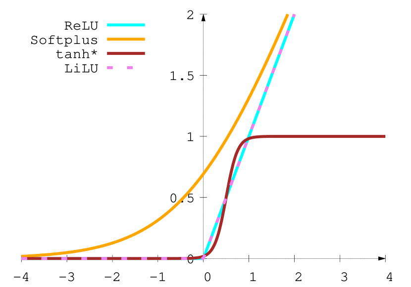
(a) Model constraints.

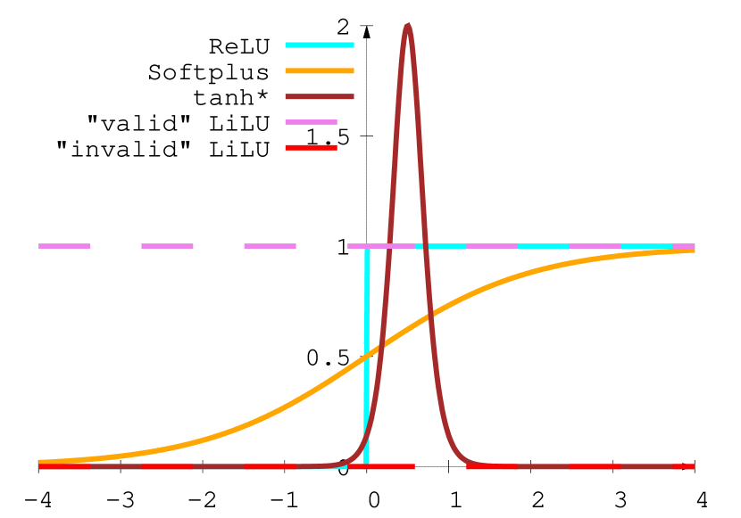
(b) Model constraints’ gradients.

Figure 3. Model constraints. 3(a)) shows multiple model constraints (activation functions) to map model unknowns to physically valid ranges. Softplus only slowly approaches zero. ReLU has no gradient for $x\leq 0$ where optimizers can easily fail. Our LiLU from Eq. 4 avoids these problems. Note that LiLU and are equal except for their gradients. 3(b)) shows LiLU’s twofold gradient which is constantly 1 for all valid optimization steps: $\lx@glossaries@gls@link{main}{LiLU}{\leavevmode LiLU}{}(x_{i})<\lx@glossaries@gls@link{main}{LiLU}{\leavevmode LiLU}{}(x_{i+1})$. However, and LiLU are both not C1-continuous. This can cause the optimizer to oscillate around $\lx@glossaries@gls@link{main}{LiLU}{\leavevmode LiLU}{}(x)=\ReLU{}(x)=0$. Our tanh variant is continuous, mostly linear and quickly approaches its borders which facilitates opacity optimization.

4.2. Surface appearance

Our SVO directly stores the ”surface appearance”. Similar to related NeRF variants, we store and optimize the outgoing radiance, i.e., the convolution of incoming light with surfaces as a volumetric and view-dependent SLF denoted by $\mathbf{L}_{o}$. Analogous to the surface geometry, the SVO stores an RGB radiance field per LoD tree level: $\mathbf{L}_{o}:^{5}\mapsto[0,\infty)^{3}$. In particular, each node stores low frequency RGB SH coefficients $\mathbf{c}_{l,m}\in^{3}$ (Ramamoorthi and Hanrahan, 2001) besides the opacity parameter. Given a 5D query $(\mathbf{x},\mathbf{v})$ for evaluating the SLF at the 3D scene location $\mathbf{x}$ and along the direction $\mathbf{v}$, we interpolate the SH coefficients of the tree nodes surrounding $\mathbf{x}$ resulting in a continuous vector field of SH coefficients $\{\mathbf{c}_{l,m}(\mathbf{x})\}$. Next, we evaluate the SH basis functions $\{Y_{l,m}\}$ with the interpolated coefficients at $\mathbf{x}{}$ for the radiance traveling direction $\mathbf{v}{}$ using their Cartesian form:

(3) $$\widehat{\mathbf{L}_{o}}(\mathbf{x},\mathbf{v})=\sum^{l=b}_{l=0}\sum^{m=l}_{m=-l}\mathbf{c}_{l,m}(\mathbf{x})\cdot Y_{l,m}(\mathbf{v})$$

whereas $\widehat{\mathbf{L}_{o}}\in^{3}$ denotes the raw, unconstrained RGB radiance, which again allows the optimizer to freely update the per-node coefficients $\{\mathbf{c}_{l,m}\}$. For memory reasons, we only store the low frequency components of the SLF in practice, i.e., the first $b{}=3{}$ bands of each color channel ($3\times b\times b{}$ coefficients per node in total).

Constraining the SLF

To compute the physically meaningful non-negative radiance $\mathbf{L}_{o}(\mathbf{x},\mathbf{v})$ after evaluating the SH basis functions for a query $(\mathbf{x},\mathbf{v})$, we map the unconstrained outgoing radiance $\widehat{\mathbf{L}_{o}}$ to $[0,\infty)$. To this end, we avoid any model constraint (activation function) producing invalid negative radiance such as leaky ReLUs, since they can introduce severe model overfitting. Also, the frequently used Softplus and both have severe disadvantages for this use case, see Fig. 3(a) and 3(b) for details. For these reasons, we introduce LiLUs (Limited Linear Units) to constrain SLF radiance (LiLU code in the supplemental). LiLUs are variants of ReLUs with pseudo gradients. I.e., their actual gradient depends on the state of the input unknown $x$ before ($x_{i}$) and after its update ($x_{i+1}$):

(4) $$\begin{split}\text{\lx@glossaries@gls@link{main}{LiLU}{\leavevmode LiLU}{}}(x)&=\begin{cases}x&\text{if }x\geq 0\\ 0&\text{otherwise}\end{cases}\\ \frac{\operatorname{d}{\text{\lx@glossaries@gls@link{main}{LiLU}{\leavevmode LiLU}{}}}(x)}{\operatorname{d}{x_{i\mapsto i+1}}}&=\begin{cases}1&\text{if }x_{i+1}\geq 0\\ 0&\text{otherwise}\end{cases}\end{split}$$

which means we practically limit the function domain to $[0,\infty)$. The gradient is zero only for update steps that would result in an invalid state: $x_{i+1}<0$; but the gradient is 1 for all valid updates, including the very border: $x_{i}=0\land x_{i+1}\geq 0$. Hence, the constrained variable is always in the physically valid function image: $\text{\lx@glossaries@gls@link{main}{LiLU}{\leavevmode LiLU}{}}(x)\geq 0$. Our LiLUs can be seen as ReLU extentions which do not suffer from complete gradient loss like ReLUs. They linearly go to zero within the physically valid range making them more suitable for optimizing low radiance surfaces than Softplus or other common constraints that slowly approach the constraint border. Note that the stored model parameters in general only go through such easy to understand constraints and not through black box compression layers, i.e., networks, which simplifies transforming scenes, e.g., for editing, see Fig. 4(a).

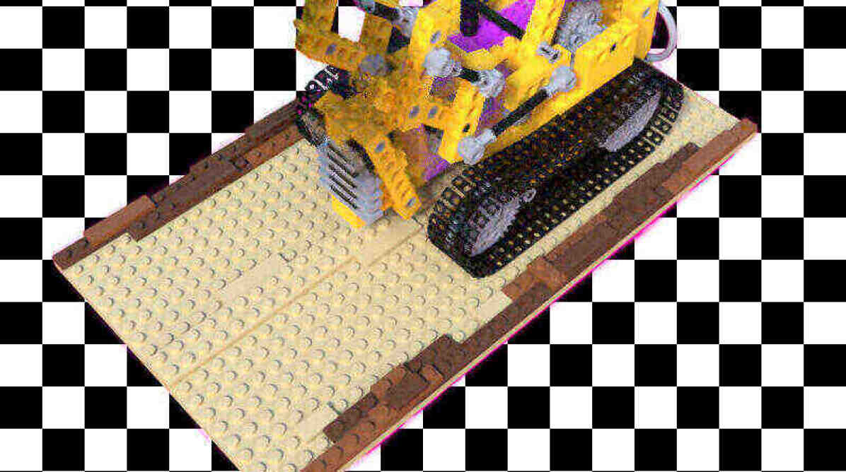
(a) Explicit scene editing.

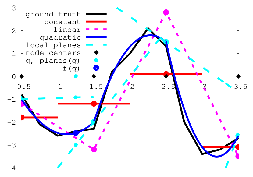
(b) Interpolation comparison.

Figure 4. (4(a)) Our representation is suited for tools such as Blender which we demonstrate using exemplary operations on the NeRF bulldozer. We switched SLF RGB channels to purple within a narrow AABB at the vehicle center and cut out an AABB volume enclosing the shovel.
(4(b)) More complex interpolation of discrete samples stored by the scene SVO to represent continuous fields is more expensive, but also achieves a better model fit as shown by the example target 1D scalar field $f$ (black). Linear interpolation (magenta) achieves a much better model fit than simple nearest neighbor lookup (red). However, our quadratic interpolation (blue) using optimized local planes (cyan) provides the best fit. The extrema of the approximating function need not coincide with the tree node centers. Quadratic interpolation for the field value $f(\mathbf{q})$ (blue dot) at the query $\mathbf{q}$ (cyan dot) entails evaluating the local planes and blending the local plane results (cyan dots) based on the distance of $\mathbf{q}$ from its surrounding nodes (black dots).

4.3. Plane-based, quadratic 4D interpolation

In order to support multi-resolution scene models which adapt to the viewing distance, we store scene data using a tree hierarchy of discrete samples to allow for 4D interpolation (spatial and LoD). In particular, our SVO stores all multi-resolution volumetric fields using local plane-based samples (function value plus spatial gradient) which we interpolate between. Specifically, an SVO stores the opacity $o:^{4}\mapsto$ and the SLF $\mathbf{L}_{o}:^{4}\mapsto^{3\times b\times b{}}$ of a scene. Each of these two multi-resolution fields is in turn composed of multiple single-resolution fields, one per tree level. Note that this same scheme can be applied to other fields as well. For example, surface materials can be attached to the SVO and interpolated in 4D analogously. In the following, we abstractly refer to such fields as $f:^{4}\mapsto^{D}$.

Our quadratic 4D field interpolation for evaluating a field $f$ as in Alg. 1, lines 1 and 1, works as follows: When processing an interpolation query $f(\mathbf{q})$ for a scale-extended scene sampling point $\mathbf{q}=[\mathbf{x}^{t}=\mathbf{r}_{i}\left(t\right),\sigma(t){}]\in^{4}$ on a view ray $\mathbf{r}_{i}$, we first compute its footprint $\sigma(t){}\in$ (spatial extend) via back projecting the diameter of the corresponding pixel $p_{i}$ along $\mathbf{r}_{i}$ to the depth $t$. Computing $f(\mathbf{q})$ then entails interpolating between the discrete local plane-based samples surrounding $\mathbf{q}$. Each tree node $j$ stores one such local plane $\pi_{n_{j}}=[f_{0}(\mathbf{x}_{j},0pt_{j}),\nabla f(\mathbf{x}_{j},0pt_{j})^{t}]\in^{4}$. The local planes are addressed using their 4D coordinates consisting of the node center and depth $(\mathbf{x}_{j},0pt_{j})$. Fig. 4(b) shows a 1D field example with 3 such plane-based samples (cyan dashed lines) and the result of blending them together (blue graph). Based on the distance $\Delta\mathbf{x}$ of $\mathbf{q}$ to the surrounding nodes (black dots), we evaluate each local plane individually (cyan dots) and blend them together for $f(\mathbf{q})$ (blue dot) using weights $w{}$. The weights $w{}$ are also based on the distance $\Delta\mathbf{x}$ (simple linear LoD and trilinear spatial interpolation) making the overall interpolation quadratic. In particular, for a single 4D point query $\mathbf{q}$, the linear blending functions $w{}$ interpolate between the local planes $\{\pi_{n_{j}}|j\in\mathcal{N}_{16}(\mathbf{q})\}$ of the 4D 16-node neighborhood $\mathcal{N}_{16}(\mathbf{q})$ surrounding $\mathbf{q}$ as follows

(5) $$\begin{split}f(\mathbf{q})&=\!\!\!\!\sum_{j\in\mathcal{N}_{16}(\mathbf{q})}\!\!\!\!{w_{\text{4D}}(\mathbf{q},\mathbf{n}_{j})\cdot\left(f_{0}(\mathbf{x}_{j},0pt_{j})+\Delta\mathbf{x}\cdot\nabla f(\mathbf{x}_{j},0pt_{j})\right)}\\ w_{\text{4D}}(\mathbf{q},\mathbf{n}_{j})&=w_{\text{LoD}}(\sigma(t){},\sigma_{j})\cdot w_{\text{3D}}(\mathbf{x},\mathbf{x}_{j})\end{split}$$

wherein $\mathbf{n}_{j}=[\mathbf{x}_{j}^{t},\sigma_{j}]\in^{4}$ depicts the center position and diameter of the neighboring tree node $j$; $\Delta_{\mathbf{x}}=(\mathbf{x}-\mathbf{x}_{j})$ is the distance vector from the node center to the 3D query position and $0pt_{j}$ is the tree depth of node $j$. The blending functions $w_{\text{3D}}{}$ and $w_{\text{LoD}}{}$ respectively provide trilinear and linear weights depending on the distance of the query within Euclidean 3D and within LoD space.

Importantly, this allows the optimizer to freely place the field extrema in 3D space despite that it updates the pairs of function samples and their local gradients ($f_{0},\nabla f)$ which are only stored at the SVO node centers. This is in contrast to only optimizing direct function samples $f_{0}$ which would only support function extrema at limited discrete node centers $\mathbf{x}_{j}$ as shown theoretically by the 1D scalar field example in Fig. 4(b). Allowing the optimizer to continuously position the field extrema (instead of fixing them to the discrete centers of the SVO nodes) is critical for fine geometry reconstruction when the initial SVO is only coarse as demonstrated by Fig. 5. For regions where the SVO is sparse, a globally constant ”border” plane $\pi_{n_{b}}$ representing free space substitutes the data of all missing neighbors.

Figure 5. Plane-based storage and interpolation of SVO fields using the ficus scene (Mildenhall et al., 2020). Given only the coarse initial SVO, linear interpolation of only function samples results in extrema fixed to voxel centers and a worse model fit (left) compared to using the spatial gradients of our local plane samples as sketched by Fig. 4(b) (right).

A single point query entails two trilinear interpolations using the blending function $w_{\text{3D}}$, each one for the scene sampling point $\mathbf{x}$ and the corresponding 8 surrounding node centers $\mathbf{x}_{j}$ at the same tree level $0pt_{j}$. We then linearly blend both 3D interpolation results along the LoD dimension of the tree using the function $w_{\text{LoD}}$. Our 4D interpolation algorithm determines the two depths $0pt_{n}$ and $(0pt_{n}-1)$ of the two surrounding 8-neighborhoods (meaning $0pt_{j}=0pt_{n}$ or $0pt_{j}=0pt_{n}-1$) according to the Nyquist sampling theorem to avoid aliasing:

(6) $$\sigma_{n}\leq\sigma(t){}<0.5\cdot\sigma_{n}$$

whereas a lower depth and thus a ”blurry” query result is returned if the tree is not deep enough for the query. Note that this LoD-aware sampling scheme is similar to sampling mipmap textures.

4.4. Background model and initial state.

Since our SVO is limited to a given scene AABB, we need to represent all captured radiance which emerged from outside the SVO. To this end, we assume that all scene parts outside the SVO are infinitely far away and model the corresponding radiance using an environment map $\mathbf{L}_{\infty}:^{2}\mapsto^{3}$ which only depends on the radiance traveling direction. Specifically, each model contains a background cube map that complements the SVO. Cube maps have the advantage of consisting of locally limited texels. This prevents oscillations during optimization, in contrast to, for example, an SH-based background for which each single frequency band parameter influences the whole background. Exactly like for the outgoing radiance $\mathbf{L}_{o}$ stored in our SVO, we constrain the distant radiance $\mathbf{L}_{\infty}$ using our LiLU-constraint. The background LiLU processes the bilinear interpolation result of the optimized cube map radiance texels.

Initial state

We initialize the background with random radiance and the opacity and radiance fields of the SVO with ”grayish fog”. The initial opacity field is mainly transparent to avoid false occlusions that would decrease convergence speed. I.e, opacity parameters are drawn from a uniform distribution, such that a ray going from the min- to the maximum scene AABB corner accumulates only up to $0.05$ total opacity. SH coefficients are respectively drawn from the uniform random distributions $[0.2475,0.5025]$ and $[-0.025,0.025]$ for band 0 and all higher bands; background radiance texels from $[0,1]$. See Fig. 1(a) for an example.

5. Rendering ERFs

To render pixels (Alg. 1 lines 1 to 1), we cast a ray $\mathbf{r}_{i}\left(t\right)=\mathbf{x}_{c,i}+t\cdot\mathbf{d}_{i}$ into the scene for each pixel $\mathbf{p}_{i}$ starting at the camera center $\mathbf{x}_{c,i}$ and going along the viewing direction $\mathbf{d}_{i}$. Our renderer gathers all the visible scene radiance along a ray from potentially multiple surfaces to estimate the RGB intensity of the corresponding pixel. For this purpose, we distribute sample points along each ray within intersected SVO nodes; filter the resulting point set multiple times to make later expensive gradient computations feasible; query the SVO fields and apply our 4D interpolation scheme, see Eq. 5 and Fig. 4(b) and accumulate the drawn samples along each ray as detailed next.

5.1. Volume rendering algorithm

The authors of NeRF (Mildenhall et al., 2020) suggested rendering scenes via an exponential transmittance function:

(7) $$\begin{split}\mathbf{L}_{p}(\mathbf{x}_{c},-\mathbf{d})&=T(t_{\infty})\cdot\mathbf{L}_{\infty}(-\mathbf{d})+\int_{t_{0}}^{t_{\infty}}{T(t)\cdot\rho(t)\cdot\mathbf{L}_{o}(t,-\mathbf{d})dt}\\ T(t)&=\exp\left(-\int_{t_{0}}^{t}{\rho(\tilde{t})d\tilde{t}}\right).\end{split}$$

This formulation is a twice adapted exponential transmittance model for volumetric rendering of participating media only absorbing or emitting radiance (Pharr et al., 2016). The traditional parts include the emitted light via the outgoing radiance field $\mathbf{L}_{o}(t,-\mathbf{d})$ and the occlusion term $T(t)$ via the extinction coefficients $\rho$. The first adaptation is by the NeRF authors who called the extinction coefficients density and they suggested to add the multiplication by the scene density $\rho$ within the outer integral and interpreted the outer integral as the expected radiance.

Note that the second adaptation of the volume rendering of Eq. 7 is by us to support a broader variety of capture setups than the NeRF formulation using $\mathbf{L}_{\infty}$. See for example the different setup of Fig. 1. The extension $\mathbf{L}_{\infty}$ adds background radiance to the model, see 4.4.

However, we find the aforementioned transmittance model unsuited for our use cases for the following reasons: First, the latter exponential transmittance model assumes that scene geometry consists of uncorrelated particles, which is not true for opaque surfaces (Vicini et al., 2021). Second, our goal is modeling soft-relaxed surfaces suited for optimization via inverse differential rendering and and also suited for approximating intricate geometry such as grass. Modeling uncorrelated particles of participating media is not our goal, but we rather estimate coverage by approximated, but structured surfaces as explained under 4.1. Observed scenes usually contain mostly free space and opaque surfaces, but not participating media. Finally, there is no scientific physical background for the mentioned density multiplication of Eq. 7. Note that Eq. 7 is also too simplistic to model participating media. For these reasons, we implemented our forward rendering model using traditional opacity compositing (alpha blending).

For each ray, we draw outgoing SLF radiance samples $\mathbf{L}_{o}(t_{i},-\mathbf{d})$ as well as opacity samples $o(t_{j})$ determining the blending weights for the totally received radiance along a ray:

(8) $$\begin{split}\mathbf{L}_{p}(\mathbf{x}_{c},-\mathbf{d})&=T(t_{\infty})\cdot\mathbf{L}_{\infty}(-\mathbf{d})+\!\!\!\sum_{i=0}^{N}{(T(t_{i})\!\!-\!\!T(t_{i+1}))\cdot\mathbf{L}_{o}(t_{i},-\mathbf{d})}\\ T(t_{i})&=\prod_{j=0}^{i-1}(1-o(t_{j}))\end{split}$$

wherein $T$ models the leftover transparency. Since view rays start close to the sensor and in free space, we set $T(t=0)$ to $1$. For traditional opacity compositing and in contrast to NeRF, $T$ directly depends on the relative surface opacity $o\in[0,1]$, see Eq. 1. Similar to layered meshes with transparency, the opacity $o$ models soft-relaxed surfaces and not filled space. It is a differentiable coverage term in contrast to discrete opaque mesh surfaces and thus more suited for optimization. However, in contrast to layered representations, the underlying geometry is continuously defined over 3D space which facilitates optimizing its exact location. Thanks to these properties, the opacity $o$ can model opaque surfaces, represent partially occluded pixels and it can also approximate intricate fine geometry such as fur, see for example Fig. 1.

Volume rendering comparison

We compared opacity compositing with the exponential transmittance model of NeRF in Fig. 6. Besides the fact that opacity compositing is simpler and cheaper to evaluate, it consistently helped the optimizer reconstruct actually opaque surfaces instead of blurry and semi-transparent results produced by the exponential transmittance model. However, the potentially more opaque opacity field $o$ is harder to optimize in case of false occlusions and thus missing gradients for occluded surfaces. To alleviate the lack of gradients leading to a correct reconstruction (besides efficiency reasons), we devised a custom scene sampling strategy for optimizing our models, which we describe in the next subsection.

Figure 6. Volume rendering comparison using the bulldozer scene (Mildenhall et al., 2020). The image rows show the bulldozer scene from (Mildenhall et al., 2020) reconstructed with MipNeRF after 1 million optimization iterations (Eq. 7); ours (a): with the same exponential transmittance and Softplus activation function (Eq. 7); ours (b): with the exponential transmittance and LiLU activation function (Eq. 7, Eq. 4); Ours (a) and (b) did not converge with density fields accurate enough for SVO node subdivisions, even after 70k optimization iterations. Ours (c): with traditional opacity compositing after 85k iterations. (Eq. 8).

5.2. Scene sampling

Efficient and robust scene sampling is critical for explicit high resolution scene reconstruction via inverse differentiable rendering. It is especially important for explicit models that are less compact than implicit neural network-based alternatives. The 3D locations of scene surfaces must be sufficiently sampled, which is difficult when their locations are initially completely unknown. For example, there need to be enough samples along each ray to not miss surfaces intersected by a ray, especially thin structures, False intermediate free space where surfaces still have to emerge during optimization also needs to be sampled densely enough. However at the same time, the number of drawn scene sampling points must be kept low to limit the costs of following rendering and gradient computations. We tackle this challenging problem using the following scene sampling scheme.

LoD-aware stratified sampling of view rays

To tackle the challenging scene sampling requirements, our renderer samples scene models via multiple steps, which Fig. 7 illustrates. First, the renderer draws uninformed samples from a uniform distribution along each ray using stratified sampling, see Alg. 1 line 1. Second, it filters samples randomly and only keeps a subset, see line 1. We exploit the fact that Adam keeps track of gradient histories. This allows for deferring dense ray sampling over multiple optimization iterations instead of densely sampling each ray within each single iteration. Third, the renderer filters the ray sampling points again after it queried the SVO for opacity samples to keep samples which are likely close to the true scene surfaces, see line 1.

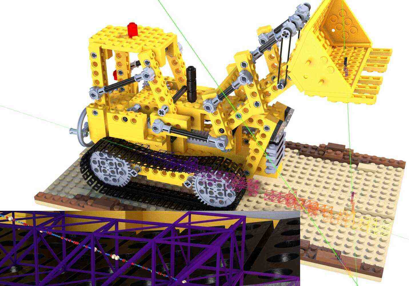
Figure 7. NeRF bulldozer scene rendering and sampling: the original Blender model overlayed with relevant SVO nodes for exemplar query rays and their sampling points. The renderer queries the scene SVO for rays (green) through 3 example input pixels at different mipmap pyramid levels. Only the intersected SVO nodes (wire frame) with side lengths fitting to the pixel back projections contain sampling points. For the ray hitting the treads, the close-up view shows the initial stratified sampling points $\left\{t_{i,j}\right\}$ (blue), the subset $\left\{t_{i,k}\right\}$ (red) from uniform random selection and finally the subset $\left\{t_{i,l}\right\}$ (white) from importance sampling used for rendering.

1. Uninformed, stratified sampling

For each ray $\mathbf{r}_{i}$, the renderer creates sampling points $\left\{t_{i,j}\right\}$ via stratified sampling, see Alg. 1 line 1; it randomly distributes these sampling points within each SVO node intersected by $\mathbf{r}_{i}$ while ensuring a sampling density that depends on the side length of the intersected node as detailed next. To account for for the projective nature of capturing devices and the spatially varying LoD within an SVO, while marching along a ray $\mathbf{r}_{i}$, the renderer goes down the SVO to nodes of depth $0pt_{n}$ with side length $\sigma_{n}$ that fit to the SVO sampling rate $\sigma(t){}$ at the current ray sampling depth $t$. In this case, the SVO sampling rate $\sigma(t)$ is the back projection of the diameter of the corresponding pixel. The ideal tree depth $0pt_{n}$ for finding the node to be sampled which has the highest LoD and is still free of aliasing is then inferred using the Nyquist sampling theorem in the same manner as for general SVO field queries via Eq. 6. If there is no tree node allocated at this depth, the corresponding ray depth interval is treated as free space. Though in the special case, if the SVO is still built up and if the traversal reached the global maximum depth of the SVO, a coarser higher level node is returned for sampling and not treated as free space. Meaning we handle the ray query with coarse nodes if not possible otherwise and with more detailed nodes at later optimization iterations. The renderer samples each node in the intersected set according to the node sizes $\left\{\sigma_{m}\right\}$ which may vary and increase with depth. In particular, for a node $n_{m}$ to be sampled, the renderer uniformly draws a constant number of $N$ samples per side length $\sigma_{m}$ within the intersection interval of $\mathbf{r}_{i}$ with $n_{m}$. The constant relative sampling density $s(n_{m})=N/\sigma_{m}$ results in a varying spatial sampling density that decreases with depth similar to inverse depth sampling. It adapts to the back projected pixel diameter $\sigma(t){}$ and according to the spatially varying available SVO LoD. The renderer filters the resulting sampling points $\left\{t_{i,j}\right\}$ next.

2. Stochastic filtering of ray sampling points

The renderer has a maximum budget for the number of sample points per ray which it enforces via deferred stochastic filtering of the sampling points $\left\{t_{i,j}\right\}$ from stratified sampling, see Alg. 1 line 1. Varying sample counts per ray are more difficult to process in parallel and storing their shading and gradients data in limited GPU memory is also more challenging compared to a capped budget for scene sampling points. Skipping sampling points randomly during optimization induces noise on the loss gradients which is per design robust against however. Also note that overall convergence is higher since intermediate false occluders are skipped randomly. They would otherwise potentially consistently occlude sampling points at the true surface locations and result in missing gradients required for correct reconstruction. Hence, the renderer randomly (uniformly) selects a subset of sampling points for each ray $\mathbf{r}_{i}$ with a sample count exceeding a given budget $N_{\text{max}}$ and produces a limited set of ray sampling points $\left\{t_{i,k}\right\}\subset\left\{t_{i,j}\right\}$.

3. Stochastic filtering of ray sampling points using opacity

The renderer then filters the already limited sampling points $\left\{t_{i,k}\right\}$ again according to the current scene geometry estimate. After querying the SVO opacity via our 4D interpolation scheme of Eq. 5 with the limited ray sampling points $\left\{t_{i,k}\right\}$, see Alg. 1 line 1, the renderer reduces the number of samples per ray using importance sampling to $N_{\text{max},o}<N_{\text{max}}$. It prefers samples $\left\{t_{i,l}\right\}\subset\left\{t_{i,k}\right\}$ which are probably close to the true surfaces. In particular, it assigns a sampling weight

(9) $$w_{s,r}(t_{i,k})=c+o(t_{i,k})$$

to each sampling point. The user-defined constant $c=0.05$ ensures that the whole ray is sampled at least infrequently to handle intermediate false free space regions. Finally, the renderer uses the two times reduced samples $\left\{t_{i,l}\right\}$ to retrieve outgoing SLF radiance samples from the SVO, see Alg. 1 line 1. We set the number of samples per node edge length to $N=8$ and limit the per-ray sample sets to $N_{\text{max}}=256$ and $N_{\text{max},o}=32$ during optimization, see the supplemental for different sample budgets. Note that this stochastic limiting is mainly required to limit the costs of the gradients computations during optimization. It is optional for only rendering once the SVO is built; when no loss gradients are computed and when the SVO nodes tightly bound the observed surfaces and thus greatly limit the ray sampling intervals.

Sampling opacity instead of density fields

Sampling along rays is simpler for opacity than for density fields. The advantage of opacity fields is they directly model the relative reduction of radiance. Each opacity sample is independent of the distance to its neighboring sampling points. This is similar to rendering fragments of layered mesh representations (Shade et al., 1998; Flynn et al., 2019; Broxton et al., 2020; Wizadwongsa et al., 2021). As opposed to this, sampling and optimizing density fields not only requires estimating correct extinction coefficients. But also finding the right step sizes between samples is critical. Nevertheless, our opacity fields can theoretically be converted to equivalent density fields.

6. Optimization

Our method iteratively reconstructs a scene model from scratch using and importance pixel sampling in a coarse to fine manner by comparing the given input images against differentiable renderings of that model from the same view and updating it according to the resulting model loss and gradients. Besides photo consistency loss from comparing renderings against the input images, we employ light priors to improve convergence, see Eq. 10. Our method starts reconstruction with a dense but coarse SVO grid that it attaches uninformed 3D fields to, see Fig. 1(a). It then mainly optimizes these fields with the SVO structure being fixed, see Fig. 1(b). Further, it infrequently updates the SVO structure to exploit free space and adapt the resolution given the current fields and then restarts field optimization for a more detailed result. see Fig. 1(c). Note that representing geometry using opacity fields is a soft relaxation similar to layered mesh representations (Shade et al., 1998). Both employ differentiable opacity parameters defining local coverage and radiance reduction directly. But otherwise, our opacity fields are continuously defined over 3D space and also provide fully differentiable surface locations like density fields (Mildenhall et al., 2020).

6.1. Objective function

During , see Alg. 1 line 1, we compute the model loss for small batches of image pixels and SVO nodes. The objective function of our optimization problem contains multiple priors besides a photo consistency term to avoid convergence at solutions that exhibit low photo consistency error, but also physically implausible surface geometry. Ambiguous reconstruction cases can cause such solutions if only photo consistency is optimized for. E.g., scenes might not have been captured sufficiently or there can be surfaces with little texture which do not sufficiently constrain their underlying geometry. To avoid these local minima, we suggest SVO priors defined on tree nodes. They prefer smooth and physically meaningful results. The priors also prevent that parameters derange if they lack correct gradients intermediately or consistently, cf. Gaussian prior on network parameters.

In particular, for a random batch of pixels $\left\{\mathbf{p}_{i}\right\}$ and random bath of SVO nodes $\left\{n_{j}\right\}$, we evaluate the objective function:

(10) $$\begin{split}l_{{\Theta}}(\left\{\mathbf{p}_{i}\right\},\left\{n_{j}\right\})=\frac{1}{|\left\{\mathbf{p}_{i}\right\}|}\sum_{i}\left[l_{p}(\mathbf{p}_{i})\right]\\ +\frac{1}{|\left\{n_{j}\right\}|}\cdot\left[l_{\text{3D}}(\left\{n_{j}\right\})+l_{\text{LoD}}(\left\{n_{j}\right\})+l_{\text{0}}(\left\{n_{j}\right\})\right]\end{split}$$

whereas the individual loss terms are as follows. The squared pixel photo consistency loss $l_{p}$ compares pixel intensity differences per color channel: $l_{p}(\mathbf{p}_{i})=\sum_{c}\|\mathcal{I}_{p}({\mathbf{p}_{i},c})-\mathcal{I}_{p}^{\text{gt}}({\mathbf{p}_{i},c})\|^{2}$. The SVO priors $l_{\text{3D}}$, $l_{\text{LoD}}$, $l_{\text{n}}$ and $l_{\text{0}}$ are losses preferring local smoothness in 3D space, local smoothness along the LoD dimension, as well as zero opacity and radiance for sparse models without clutter.

The photo consistency and prior losses are both normalized by their individual batch size for comparability. We set the batch size to $4096$ for both batch types in our experiments (pixels and nodes). Note that we also employed background priors enforcing local smoothness and zero radiance. They are analogous to the their SVO counterparts and thus we omit them here for brevity.

SVO priors

The objective function contains the following priors:

(11) $$l_{\text{3D}}(\left\{n_{j}\right\}) =\lambda_{\text{3D}}\cdot\sum_{n_{j}}\sum_{n_{k}\in\mathcal{N}_{6}(n_{j})}l_{1}(f(\mathbf{x}_{j},0pt_{j})-f(\mathbf{x}_{k},0pt_{j}))$$

(12) $$l_{\text{LoD}}(\left\{n_{j}\right\}) =\lambda_{\text{LoD}}\cdot\sum_{n_{j}}{l_{1}(f(\tilde{\mathbf{x}}_{j},0pt_{j})-f(\tilde{\mathbf{x}}_{j},0pt_{j}+1))}$$

(13) $$l_{\text{0}}(\left\{n_{j}\right\}) =\lambda_{\text{0}}\cdot\sum_{n_{j}}{l_{1}(f(\tilde{\mathbf{x}}_{j},0pt_{j}))}$$

which regularize the SVO node parameters. Eq. 11 prefers local smoothness. Eq. 12 enforces smoothness between tree levels. Eq. 13 punishes deranging parameters by preferring zero density and radiance. Note that we applied the SVO priors to the opacity $o$ and the outgoing radiance field $\mathbf{L}_{o}$. We also analogously applied local smoothness and low radiance priors to the background cube map texels which we omit here for brevity. Hereby, $\mathcal{N}_{6}(n_{j})$ are the six axis aligned neighbors of node $n_{j}$; $l_{1}$ is the smooth Huber loss function; $\mathbf{x}_{j}$ is the center of node $n_{j}$; $\tilde{\mathbf{x}}_{j}$ is a random 3D position within the scope of node $j$ and $0pt_{j}$ is its depth within the tree. We choose the nodes $\left\{n_{j}\right\}$ to which the priors are applied as detailed next. Further, we uniformly set the strength of all priors via $\lambda=1e-3$ for all the experiments shown here (supplemental material with varying $\lambda$ experiment).

Stochastic priors

Our stochastic priors improve convergence via normalized random batches. For the SVO priors, we simply randomly choose SVO nodes (and neighborhoods). We directly apply the rendering priors to the rays of the random input pixel batches (that are already available for reducing photo consistency errors). The priors hence similarly work to the data term that is based on the random input pixel batches. Applying the priors every iteration to every ray or voxel would result in very consistent and hence overly strong priors. Contrary, our random prior batches facilitate convergence, but are also treated as noisy outliers in cases where they do not fit, since the stochastic priors are tracked like the data term by Adam’s gradient histories. E.g., applying local smoothness to an edge infrequently results in wrong, but inconsistent gradients Adam is robust against. Additionally, the costs of our stochastic priors scale with the batch and not the model size making them more suitable for complex models with many parameters.

Suitable optimizer.

We investigated different solvers for fitting our scene models against registered images of a scene. Higher order solvers such as Levenberg-Marquardt optimization algorithm (Moré, 1978) (LM), limited-memory BFGS (LBFGS) or preconditioned conjugate gradients (PCG) were either too expensive given the high number of unknowns of our scene models or they failed to reconstruct scenes from scratch. That means they converged in a bad local optimum due to our optimization problems being highly non-convex and due to starting far from the globally optimal solution while making simplifying assumptions to approximate the inverse Hessian which are not applicable in our case. So we eventually decided for a relatively cheap -based optimizer which is still powerful enough for the targeted non-convex and high-dimensional objective functions. I.e., we employed Adam for all our experiments and ran it with the recommended settings (Kingma and Ba, 2014).

Figure 8. Intermediate ficus scene (Mildenhall et al., 2020) models after optimizing the SVO fields given the initial dense SVO (left) and given the SVO sparsified after 30k mini batch iterations (right).

6.2. Hierarchical optimization

Our method reconstructs scene models in a coarse to fine manner. It starts with a dense, but coarse scene grid, i.e., a full, shallow SVO. The tree then gradually becomes sparser by merging of nodes or more detailed thanks to new leaves. The SVO structure changes infrequently depending on its attached fields after optimizing them for a fixed SVO structure as shown by the outer loop of Alg. 1.

Merging SVO nodes.

We merge nodes in free space to save memory and reduce rendering costs. Merging nodes also considerably increases the quality of the view ray sampling point distributions as demonstrated by Fig. 8. By means of the optimized opacity field $o$, we determine the set of nodes $\left\{n_{r}\right\}$ required for rendering using Dijkstra searches that we run on each tree level’s 27-neighborhood graph. The Dijkstra search is hysteresis-based similarly to the Canny edge detector (Canny, 1986) for robustness. First, we sample each tree node using a regular pattern of $8^{3}$ sampling points and determine its maximum opacity $o_{\text{max}}(j)$. Second, we start a Dijkstra search on each unvisited node $j$ with $o_{\text{max}}(j)\geq 0.75$ and only expand the search to nodes $\{k\}$ with $o_{\text{max}}(k)\geq 0.075$. Third, a 27-neighborhood dilation augments the set of all visited nodes to ensure complete opacity function ramps from free to occupied space The resulting set of $\left\{n_{r}\right\}$ then defines nodes which must not be discarded: We either keep all 8 children of an SVO node if any child is within $\left\{n_{r}\right\}$ or discard all of them, which is similar to the work (Laine and Karras, 2010).

Subdividing SVO nodes.

To subdivide nodes, we first find the set of required nodes $\left\{n_{r}\right\}$ in the same manner as for merging. However, a leaf node within $\left\{n_{r}\right\}$ is only eligible for subdivision if the subdivision does not induces under sampling. That means there must be an input pixel with small enough 3D footprint such that the Nyquist sampling theorem still holds (similar to Eq. 6). The footprint $\sigma(t){}$ from back projecting the pixel to the depth $t$ of the node defines the sampling rate and the node edge length defines the signal rate. If a leaf is within $\left\{n_{r}\right\}$ and does not induce aliasing, we allocate all of its 8 children. The SVO fills all new leaf nodes with the 3D-interpolated data of their parents resulting in a smooth initialization with less block artifacts compared to copying parent values. Our method afterwards optimizes the new and smoothed, but also more detailed SVO using again as denoted in the inner loop of Alg. 1. The refinement finally stops if there are no new leaf nodes according to the Nyquist sampling theorem.

6.3. Input pixel sampling for

To facilitate convergence, our method employs Gaussian pyramids of the input images and importance sampling as described next.

For better optimization convergence and before the actual optimization, we compute a complete Gaussian (mipmap) pyramid of each input image. We then randomly select pixels from all input image pyramids to simultaneously optimize the whole SVO at multiple levels of detail. Coarser input pixels from higher mipmap levels have a larger footprint and thus help optimize inner or higher level SVO nodes as in the sampling scheme of Eq. 6.

Importance sampling

For faster convergence where scene reconstruction has not finished yet, we implemented importance sampling. We prefer pixels with high photo consistency error as depicted by Alg. 1 line 1 and demonstrated using Fig. 9. The sampling weights are basically the per-pixel maxima of the color channel errors: $w_{s,p}(\mathbf{p}_{i})=\max_{c}(\|\mathcal{I}_{p}({\mathbf{p}_{i},c})-\mathcal{I}_{p}^{\text{gt}}({\mathbf{p}_{i},c})\|^{2})+c$. Similarly to the ray sampling of Eq. 9, we add a small constant $c=0.05$ to also sample low error pixels infrequently and prevent oscillating errors. To implement this scheme, a loss cache $\mathcal{C}$ steers the importance sampler, see line 1. It caches running error averages of the input pixels via the photo consistency loss of the pixel batches $\left\{l_{p}(\mathbf{p}_{i})\right\}$, see line 1. The cache stores prefix sum offsets of the sampling weights $\left\{w_{s,p}(\mathbf{p}_{i})\right\}$ for fast random pixel selection whereas it updates these offsets infrequently, i.e., every $5000$ iterations. Further, we only store coarse error cache data, meaning only at higher image mipmap pyramid levels for efficiency reasons and to broaden the image sampling area of the importance sampler. If a low mipmap level is selected where multiple fine pixels fall into the same coarse pixel with a single running average error, then the sampler uniformly selects between all fine pixels.

Figure 9. Pixel sampling comparison using the NeRF room scene (Mildenhall et al., 2020) for a test view after 175k iterations.

7. Results

In the following, we evaluate individual contributions of our approach and show that our reconstructed explicit models are comparable to state-of-the-art implicit alternatives. Our models converge faster in general, but their implicit competitors generally converge at the best solutions after many more iterations.

Volume rendering algorithms.

We compared direct opacity compositing against the exponential transmittance formulation from (Mildenhall et al., 2020). When employing the exponential transmittance formulation (Eq. 7), our explicit model are less accurate compared to their opacity compositing-based alternatives from (Eq. 8). The density field is smeared out and much blurrier than the opacity field. The density fields are also less suited for our hierarchical refinement as empty nodes are more difficult to distinguish from SVO nodes in occupied space. Interestingly, the MLP representation of MipNeRF is not affected in the same way. The MipNeRF models of the synthetic scenes have low photo consistency error and accurate underlying geometry despite the exponential transmittance model. However, the MipNeRF models need many more mini batch optimization iterations.

Ablation study.

First, the comparison of Fig. 5 demonstrates the importance of our quadratic 4D interpolation when sampling scenes for scale-augmented 3D points. Interpolating between local planes (field function samples plus local gradients) allows the optimizer to select continuous instead of limited discrete 3D positions for the extrema of the fields. It hence better fits the scene model to the input images when voxels are only coarse. This is especially beneficial for fine and intricate geometry like from the shown ficus. Second, the error-driven importance sampling improves convergence as demonstrated by Fig. 9.

Qualitative evaluation

Fig. 10 shows reconstruction for exemplary synthetic scenes from NeRF (Mildenhall et al., 2020) where our method performs similar to MipNeRF. Note that our algorithm is able to reconstruct many of the fine and thin structures like the ship ropes despite that it starts with a coarse grid only. Fig. 11 demonstrates that our approach can also reconstruct large scale outdoor scenes with complex scene geometry. Though, our models exhibit fewer details than JaxNeRF (improved original NeRF).

Figure 10. Qualitative evaluation using MipNeRF and ours on the synthetic chair and ship scene (Mildenhall et al., 2020) with (from left to right): original hold-out ground truth image; photo-realistic reconstruction; density (MipNeRF) or opacity (ours); surface normals and depth map visualization.

Figure 11. Qualitative evaluation using JaxNeRF and ours on the leaves and orchid scene (Mildenhall et al., 2019) with (from left to right): original hold-out ground truth images; photo-realistic reconstructions (JaxNeRF and ours); renderings of opacity, surface normals and depths (ours only).

Quantitative evaluation

Tab. 2 shows that our method reconstructs high quality models that are similar to the state-of-the-art implicit MipNeRF approach. Our models perform slightly worse due to view ray sampling noise and due to the fact that they cannot capture high-frequency reflections well. We omit a qualitative comparison against JaxNeRF on the LLFF scenes. Our models consistently perform worse mainly due to the limiting initial SVO creation and due to the fact that we do not dynamically adapt the user-defined scene AABB. Fig. 12 shows that our method reconstructs the object of interest inside the scene AABB. However, it is surrounded by clutter that the optimizer added to account for the table outside the AABB which cannot be represented well by the environment map.

Figure 12. Fortress scene (Mildenhall et al., 2019) reconstruction after 170k iterations based on a manually defined tight scene AABB.

	PSNR$\uparrow$		SSIM$\uparrow$
	MipNeRF	ours	MipNeRF	ours
Chair	35.19	28.73	0.9891	0.9887
Drums	26.16	24.22	0.9597	0.9657
Ficus	32.34	27.36	0.9861	0.9864
Hot dog	37.18	31.71	0.9921	0.9883
Bulldozer	35.76	28.38	0.9903	0.9817
Materials	31.50	26.29	0.9808	0.9662
Mic	36.22	30.23	0.9941	0.9888
Ship	29.33	25.38	0.9297	0.9409
Average	32.96	27.79	0.9777	0.9758

Table 2. Quantitative novel view synthesis comparison of the proposed explicit models (ours) with MipNeRF (Barron et al., 2021) on the synthetic NeRF scenes (Mildenhall et al., 2020).

8. Conclusion

Limitations and future work

First, the biggest limitation of our method is the simple initial SVO creation. If the assumption is broken that the geometry outside the AABB is infinitely far away, the optimizer creates ”clutter” in free space. If the AABB is initially very big, either the voxels are too coarse or the dense initial grid consumes too much memory for fine voxels. A solution would be creating the dense SVO according to the camera distribution and dynamically adding new root nodes during optimization if necessary. Second, using only SHs to store the outgoing radiance of scene surfaces limits them to low frequency radiance distributions. Hence, our representation fails to capture sharp highlights for shiny materials. E.g., the water reflections of the NeRF ship scene are such a failure case. Investigating different ways to represent hemispherical radiance distributions within our models, e.g., using kernel-based methods, is an interesting future direction. Third, directly optimizing the SLF ”bakes the scene light” into the surfaces. This reduces model flexibility and for example possibilities for further editing. E.g., in case of the bulldozer scene of Fig. 4(a), it is desirable to not only remove the shovel, but also the shadow it casts onto the vehicle. However, decomposing SLFs into incoming radiance and surface materials seems possible since their convolution is also differentiable and can be optimized using . Though, this is a very complex and ambiguous problem, which is out of scope of this work, but also promising for future research.

Summary

In this work, we presented a novel representation which explicitly represents a 3D scene using a sparse multi-resolution grid storing surface geometry statistically via an opacity field and the radiance outgoing from this surface geometry via a volumetric SH SLF. Further, we showed how to initialize and optimize such a scene model in a coarse-to-fine manner using and inverse differentiable rendering for multiple views. Finally, we provided reconstruction results comparable to state-of-the-art approaches regarding novel view synthesis and demonstrated the advantages of our novel approach regarding its versatility for capturing as well as its suitability for post processing use cases, such as interactive editing.

Appendix A Supplementary material

In the following, we show additional results for specific parts of our method like changing model parameters, such as the SH band count, as well as more quantitative and qualitative comparisons of our method against state-of-the-art implicit alternatives. Also we show how simple our LiLU constraints are using their full PyTorch (Paszke et al., 2019) code:

import torch

class LiLU(torch.autograd.Function):
    @staticmethod
    def forward(
        ctx, x: torch.Tensor
    ) -> torch.Tensor:
        ctx.border = x.le(0.0)
        y = x.masked_fill(ctx.border, 0.0)
        return y

    @staticmethod
    def backward(
        ctx, g_y: torch.Tensor
    ) -> torch.Tensor:
        if not ctx.needs_input_grad[0]:
            return (None,)



        # shrinking?
        # (assuming loss minimization)
        s = g_y > 0.0
        # and at border?
        b = ctx.border
        # not okay
        no = torch.logical_and(b, s)
        g_in = g_y.masked_fill(no, 0.0)
        return (g_in,)

Tab. 3 compares our approach regarding Learned Perceptual Image Patch Similarity (Zhang et al., 2018) (LPIPS) on the NeRF scenes where MipNeRF performs better.

LPIPS$\downarrow$	MipNeRF	ours
Chair	0.013	0.036
Drums	0.064	0.072
Ficus	0.021	0.045
Hot dog	0.020	0.061
Bulldozer	0.015	0.043
Materials	0.027	0.078
Mic	0.006	0.027
Ship	0.128	0.183
Average	0.0367	0.0679

Table 3. LPIPS comparison using the proposed explicit models (ours) with MipNeRF (Barron et al., 2021) on the scenes from (Mildenhall et al., 2020).

Fig. 13 shows differences in reconstruction quality for varying numbers of SH bands to represent outgoing surface radiance. Increasing the SH band count first increases reconstruction quality. However, the quality decreases again starting with 4 bands. We presume that optimization convergence decreases due to the higher degree of the underlying polynomials which are not localized in angular space. The frequency-based design of the SHs presumably compounds optimization as each drawn radiance sample gradient influences all SH coefficients.

Figure 13. SH band count comparison with reconstructed models after 30k mini batch iterations on the synthetic materials scene (Mildenhall et al., 2020) (from left to right): hold-out ground truth image (gt), photo-realistic reconstruction, opacity, surface normals and depth map.

Fig. 14 compares reconstruction results for varying prior strengths. They induce overly smooth results for $\lambda=0.1$ and $\lambda=0.01$ and have almost no impact for $\lambda=1e-4$. Note that the zero opacity prior also reduces the initial clutter in free space more for higher $\lambda$ values. Thus, we generally set $\lambda=1e-3$ for our experiments.

Figure 14. Varying prior strengths experiment showing Lion reconstructions after 50k iterations with decreasing $lambda$ factors and thus also decreasing model smoothness and increasing free space clutter from top to bottom.

We investigated the influence of different sampling budgets during optimization. Fig. 15 and Fig. 16 demonstrate that Adam is very robust against the noise introduced by only small sampling budgets. Interestingly, the reconstructions are actually better (less false clutter in free space) when only employing smaller and cheaper sampling budgets. We presume that small sampling budgets increase the probability of sampling around false occluders which mitigates the lack of required gradients they induce on occluded voxels. Note that smaller sampling budgets partially blur the fields and result in voxels within objects being occupied despite our zero opacity prior. Uniform instead of stratified sampling within a ray-intersected node (4th row only) reduces reconstruction quality only little in this case.

Figure 15. Scene sampling influence on early results of the Lion scene with varying sampling budgets $N/N_{\text{max}}/N_{\text{max},o}$ which respectively are the samples per node edge length; maximum number of samples per ray after uninformed and after opacity-based filtering.

Figure 16. Scene sampling influence on results of the Lion scene after 40k iterations and with varying sampling budgets $N/N_{\text{max}}/N_{\text{max},o}$.

The overview of Fig. 17 demonstrates the novel view synthesis performance of our method for all of the synthetic NeRF scenes (Mildenhall et al., 2020). Our method reconstructs the scenes within comparably few optimization iterations and with high quality that is similar to state-of-the-art implicit approaches like MipNeRF. However, the surface light field based on low frequency SHs is clearly not able to represent sharp reflections as for example the drums scene comparison shows.

Figure 17. Qualitative evaluation using an overview of our results for all of the synthetic NeRF scenes (Mildenhall et al., 2020).

We tested the robustness of our method against fine details with opposing surface radiance (black and white checker pattern) using the synthetic checkered cube scene shown in Fig. 18. Our method is able to reconstruct the checker pattern and does not fail with a average gray surface estimate despite the -based optimization.

Figure 18. Robustness experiment on a synthetic scene consisting of an axis-aligned checkered cube flying inside a beach environment map showing (left to right): hold out ground truth; photo realistic reconstruction; photo consistency errors; surface normals and depths.

References

- (1)
- Aroudj et al. (2017) Samir Aroudj, Patrick Seemann, Fabian Langguth, Stefan Guthe, and Michael Goesele. 2017. Visibility-Consistent Thin Surface Reconstruction Using Multi-Scale Kernels. ACM TOG 36, 6 (Sept. 2017), 187:1–187:13. http://tubiblio.ulb.tu-darmstadt.de/89320/
- Barron et al. (2021) Jonathan T. Barron, Ben Mildenhall, Matthew Tancik, Peter Hedman, Ricardo Martin-Brualla, and Pratul P. Srinivasan. 2021. Mip-NeRF: A Multiscale Representation for Anti-Aliasing Neural Radiance Fields. arXiv:2103.13415 [cs.CV] https://jonbarron.info/mipnerf/
- Bi et al. (2020a) Sai Bi, Zexiang Xu, Pratul Srinivasan, Ben Mildenhall, Kalyan Sunkavalli, Miloš Hašan, Yannick Hold-Geoffroy, David Kriegman, and Ravi Ramamoorthi. 2020a. Neural Reflectance Fields for Appearance Acquisition. arXiv:2008.03824 [cs.CV]
- Bi et al. (2020b) Sai Bi, Zexiang Xu, Kalyan Sunkavalli, Milos̆ Has̆an, Yannick Hold-Geoffroy, David Kriegman, and Ravi Ramamoorthi. 2020b. Deep Reflectance Volumes: Relightable Reconstructions from Multi-View Photometric Images. In European Conference on Computer Vision (ECCV 2020). https://arxiv.org/abs/2007.09892
- Boss et al. (2021) Mark Boss, Raphael Braun, Varun Jampani, Jonathan T. Barron, Ce Liu, and Hendrik P.A. Lensch. 2021. NeRD: Neural Reflectance Decomposition from Image Collections. In ICCV.
- Broxton et al. (2020) Michael Broxton, John Flynn, Ryan Overbeck, Daniel Erickson, Peter Hedman, Matthew DuVall, Jason Dourgarian, Jay Busch, Matt Whalen, and Paul Debevec. 2020. Immersive Light Field Video with a Layered Mesh Representation. ACM Transactions on Graphics (Proc. SIGGRAPH) 39, 4 (2020), 86:1–86:15.
- Canny (1986) John Canny. 1986. A Computational Approach to Edge Detection. IEEE Trans. Pattern Anal. Mach. Intell. 6 (1986), 679–698.
- Curless and Levoy (1996) Brian Curless and Marc Levoy. 1996. A Volumetric Method for Building Complex Models from Range Images. In SIGGRAPH.
- Flynn et al. (2019) John Flynn, Michael Broxton, Paul Debevec, Matthew DuVall, Graham Fyffe, Ryan Styles Overbeck, Noah Snavely, and Richard Tucker. 2019. DeepView: High-quality View Synthesis by Learned Gradient Descent. In CVPR. https://arxiv.org/abs/1906.07316
- Gortler et al. (1996) Steven J. Gortler, Radek Grzeszczuk, Richard Szeliski, and Michael F. Cohen. 1996. The Lumigraph. In SIGGRAPH (SIGGRAPH ’96). Association for Computing Machinery, Inc., New York, NY, USA, 43–54. https://doi.org/10.1145/237170.237200
- Hedman et al. (2021) Peter Hedman, Pratul P. Srinivasan, Ben Mildenhall, Jonathan T. Barron, and Paul Debevec. 2021. Baking Neural Radiance Fields for Real-Time View Synthesis. ICCV (2021).
- Hoppe et al. (1992) Hugues Hoppe, Tony DeRose, Tom Duchamp, John McDonald, and Werner Stuetzle. 1992. Surface Reconstruction from Unorganized Points. In SIGGRAPH.
- Kellnhofer et al. (2021) Petr Kellnhofer, Lars Jebe, Andrew Jones, Ryan Spicer, Kari Pulli, and Gordon Wetzstein. 2021. Neural Lumigraph Rendering. In CVPR. http://www.computationalimaging.org/publications/nlr/
- Kingma and Ba (2014) Diederik P. Kingma and Jimmy Ba. 2014. Adam: A Method for Stochastic Optimization. arXiv:1412.6980 [cs.LG]
- Laine and Karras (2010) Samuli Laine and Tero Karras. 2010. Efficient Sparse Voxel Octrees – Analysis, Extensions, and Implementation. NVIDIA Corporation 2 (2010).
- Liu et al. (2020) Lingjie Liu, Jiatao Gu, Kyaw Zaw Lin, Tat-Seng Chua, and Christian Theobalt. 2020. Neural Sparse Voxel Fields. Advances in Neural Information Processing Systems (2020).
- Liu et al. (2021) Steven Liu, Xiuming Zhang, Zhoutong Zhang, Richard Zhang, Jun-Yan Zhu, and Bryan Russell. 2021. Editing Conditional Radiance Fields. In ICCV.
- Lombardi et al. (2019) Stephen Lombardi, Tomas Simon, Jason Saragih, Gabriel Schwartz, Andreas Lehrmann, and Yaser Sheikh. 2019. Neural Volumes: Learning Dynamic Renderable Volumes from Images. ACM Trans. Graph. 38, 4, Article 65 (July 2019), 14 pages.
- Luan et al. (2021) Fujun Luan, Kavita Bala, and Zhao Dong. 2021. Unified Shape and SVBRDF Recovery using Differentiable Monte Carlo Rendering. In Proceedings IEEE Conf. on Computer Vision and Pattern Recognition (CVPR).
- Martel et al. (2021) Julien N.P. Martel, David B. Lindell, Connor Z. Lin, Eric R. Chan, Marco Monteiro, and Gordon Wetzstein. 2021. ACORN: Adaptive Coordinate Networks for Neural Representation. ACM TOG (2021).
- Martin-Brualla et al. (2021) Ricardo Martin-Brualla, Noha Radwan, Mehdi S. M. Sajjadi, Jonathan T. Barron, Alexey Dosovitskiy, and Daniel Duckworth. 2021. NeRF in the Wild: Neural Radiance Fields for Unconstrained Photo Collections. In CVPR.
- Mildenhall et al. (2019) Ben Mildenhall, Pratul P. Srinivasan, Rodrigo Ortiz-Cayon, Nima Khademi Kalantari, Ravi Ramamoorthi, Ren Ng, and Abhishek Kar. 2019. Local Light Field Fusion: Practical View Synthesis with Prescriptive Sampling Guidelines. ACM TOG (2019). https://bmild.github.io/llff/
- Mildenhall et al. (2020) Ben Mildenhall, Pratul P. Srinivasan, Matthew Tancik, Jonathan T. Barron, Ravi Ramamoorthi, and Ren Ng. 2020. NeRF: Representing Scenes as Neural Radiance Fields for View Synthesis. In European Conference on Computer Vision (ECCV 2020). arXiv:2003.08934 [cs.CV]
- Moré (1978) Jorge J. Moré. 1978. The Levenberg-Marquardt algorithm: Implementation and theory. In Numerical Analysis, G. A. Watson (Ed.). Springer Berlin Heidelberg, Berlin, Heidelberg, 105–116.
- Paszke et al. (2019) Adam Paszke, Sam Gross, Francisco Massa, Adam Lerer, James Bradbury, Gregory Chanan, Trevor Killeen, Zeming Lin, Natalia Gimelshein, Luca Antiga, Alban Desmaison, Andreas Kopf, Edward Yang, Zachary DeVito, Martin Raison, Alykhan Tejani, Sasank Chilamkurthy, Benoit Steiner, Lu Fang, Junjie Bai, and Soumith Chintala. 2019. PyTorch: An Imperative Style, High-Performance Deep Learning Library. In Advances in Neural Information Processing Systems 32, H. Wallach, H. Larochelle, A. Beygelzimer, F. d'Alché-Buc, E. Fox, and R. Garnett (Eds.). Curran Associates, Inc., 8024–8035. http://papers.neurips.cc/paper/9015-pytorch-an-imperative-style-high-performance-deep-learning-library.pdf
- Pharr et al. (2016) Matt Pharr, Wenzel Jakob, and Greg Humphreys. 2016. Physically based Rendering: From Theory to Implementation. Morgan Kaufmann.
- Ramamoorthi and Hanrahan (2001) Ravi Ramamoorthi and Pat Hanrahan. 2001. An Efficient Representation for Irradiance Environment Maps. In Proceedings of the 28th Annual Conference on Computer Graphics and Interactive Techniques (SIGGRAPH ’01). Association for Computing Machinery, 497–500.
- Reiser et al. (2021) Christian Reiser, Songyou Peng, Yiyi Liao, and Andreas Geiger. 2021. KiloNeRF: Speeding up Neural Radiance Fields with Thousands of Tiny MLPs. ICCV (2021).
- Seitz and Dyer (1999) S. M. Seitz and C. M. Dyer. 1999. Photorealistic Scene Reconstruction by Voxel Coloring. International Journal of Computer Vision (IJCV) 35, 2 (Nov. 1999), 151–173.
- Shade et al. (1998) Jonathan Shade, Steven Gortler, LW He, and Richard Szeliski. 1998. Layered depth images. In SIGGRAPH. https://grail.cs.washington.edu/projects/ldi/
- Srinivasan et al. (2021) Pratul P. Srinivasan, Boyang Deng, Xiuming Zhang, Matthew Tancik, Ben Mildenhall, and Jonathan T. Barron. 2021. NeRV: Neural Reflectance and Visibility Fields for Relighting and View Synthesis. In CVPR.
- Szeliski and Golland (1999) Rick Szeliski and Polina Golland. 1999. Stereo Matching with Transparency and Matting. IJCV 32, 1 (1999), 45–61. http://users.eecs.northwestern.edu/~yingwu/teaching/EECS432/Reading/Szeliski_IJCV99.pdf
- Turk and Levoy (1994) Greg Turk and Marc Levoy. 1994. Zippered Polygon Meshes from Range Images. In SIGGRAPH.
- Vicini et al. (2021) Delio Vicini, Wenzel Jakob, and Anton Kaplanyan. 2021. A Non-Exponential Transmittance Model for Volumetric Scene Representations. ACM TOG 40, 4 (Aug. 2021), 136:1–136:16. https://doi.org/10.1145/3450626.3459815
- Wizadwongsa et al. (2021) Suttisak Wizadwongsa, Pakkapon Phongthawee, Jiraphon Yenphraphai, and Supasorn Suwajanakorn. 2021. NeX: Real-time View Synthesis with Neural Basis Expansion. In IEEE Conference on Computer Vision and Pattern Recognition (CVPR).
- Yang et al. (2021) Guandao Yang, Serge Belongie, Bharath Hariharan, and Vladlen Koltun. 2021. Geometry Processing with Neural Fields. Advances in Neural Information Processing Systems 34 (2021).
- Yariv et al. (2020) Lior Yariv, Yoni Kasten, Dror Moran, Meirav Galun, Matan Atzmon, Ronen Basri, and Yaron Lipman. 2020. Multiview Neural Surface Reconstruction by Disentangling Geometry and Appearance. Advances in Neural Information Processing Systems (2020).
- Yu et al. (2021) Alex Yu, Ruilong Li, Matthew Tancik, Hao Li, Ren Ng, and Angjoo Kanazawa. 2021. PlenOctrees for Real-time Rendering of Neural Radiance Fields. In ICCV.
- Zhang et al. (2021a) Kai Zhang, Fujun Luan, Qianqian Wang, Kavita Bala, and Noah Snavely. 2021a. PhySG: Inverse Rendering with Spherical Gaussians for Physics-based Material Editing and Relighting. arXiv:2104.00674 [cs.CV]
- Zhang et al. (2020) Kai Zhang, Gernot Riegler, Noah Snavely, and Vladlen Koltun. 2020. NeRF++: Analyzing and Improving Neural Radiance Fields. arXiv:2010.07492 [cs.CV]
- Zhang et al. (2018) Richard Zhang, Phillip Isola, Alexei A Efros, Eli Shechtman, and Oliver Wang. 2018. The Unreasonable Effectiveness of Deep Features as a Perceptual Metric. In CVPR.
- Zhang et al. (2021b) Xiuming Zhang, Pratul P Srinivasan, Boyang Deng, Paul Debevec, William T Freeman, and Jonathan T Barron. 2021b. NeRFactor: Neural Factorization of Shape and Reflectance Under an Unknown Illumination. arXiv preprint arXiv:2106.01970 (2021).
- Zhou et al. (2018) Tinghui Zhou, Richard Tucker, John Flynn, Graham Fyffe, and Noah Snavely. 2018. Stereo Magnification: Learning View Synthesis using Multiplane Images. In SIGGRAPH.