QCD Analysis of $\Delta S=0$ Hadronic Parity Violation

Abstract

We present a QCD analysis of the effective weak Hamiltonian at hadronic energy scales for strangeness-nonchanging ($\Delta S=0$) hadronic processes. Performing a leading-order renormalization group analysis in QCD from the $W$ to the ${\cal O}(2\,\rm GeV)$ energy scale, we derive the pertinent effective Hamiltonian for hadronic parity violation, including the effects of both neutral and charged weak currents. We compute the complete renormalization group evolution of all isosectors and the evolution through heavy-flavor thresholds for the first time. We show that the additional four-quark operators that enter below the $W$ mass scale from QCD operator mixing effects form a closed set, and they result in a 12×12 anomalous dimension matrix. Computing the resulting effective Hamiltonian and comparing to earlier results, we affirm the importance of operator mixing effects and find, as an example, that the parity-violating pion-nucleon coupling constant, using the factorization Ansatz and an assessment of the pertinent quark charge of the nucleon in lattice QCD at the 2 GeV scale, is in better agreement with recent experiments.

1 Introduction

In the Standard Model (SM), the observed failure of parity conservation in the low-energy interactions of nucleons and nuclei follows from a subtle interplay of electroweak and strong interaction effects, with the nonperturbative nature of the strong interaction acting to confound the theoretical interpretation of the effects observed thus far. The low-energy nature of these studies has meant that its theoretical description has focused on phenomenological realizations in hadronic degrees of freedom, with the long-held expectation that the charged pion exchange interaction should strongly dominate [1]. Despite the small mass of the pion relative to the $1\,\rm GeV$ scale, this has not proven to be the case; rather, isoscalar and isotensor interactions, also appear to play important phenomenological roles [2, 3, 4, 5, 6].

Direct theoretical insight on the relative importance of isoscalar, isotensor, and isovector parity-violating nucleon-nucleon (NN) interactions has come from the analysis of NN amplitudes in pionless effective field theory (EFT) in the large number of colors ($N_{c}$) limit [7, 2, 3]. In this paper we revisit this issue within a framework that makes direct contact to the degrees of freedom of the Standard Model (SM) Lagrangian. That is, starting with the effective, flavor-conserving, parity-violating Hamiltonian of quarks apropos to NN interactions at the weak scale, we use renormalization group techniques, including leading-order (LO) QCD evolution and operator mixing effects, matching across heavy-quark thresholds, to determine the effective weak Hamiltonian for $u,d$, and $s$ quarks at the $2\,\rm GeV$ scale. Work of this kind exists in the literature, starting with that of Ref. [1], though the existing work has either made additional calculational approximations [1, 8, 9] or has specialized to the isovector case [10, 11, 12]. In this work we consider all three isosectors, and since the renormalization group effects we consider respect isospin symmetry, we separate the problem as illustrated in Fig. 1 — we can determine the isospin-separated effective Hamiltonian just below the $W$ mass scale and evolve it to hadronic scales or we can evolve the full effective Hamiltonian and effect the isospin separation at the same low-energy scale and find the same result. As an application, we use our weak effective Hamiltonian we have constructed to compute the parity-violating pion-NN coupling constant that appears in the parity-violating Hamiltonian of Desplanques, Donoghue, and Holstein (DDH) [1], to find improved agreement with experimental results.

Figure 1: Illustration of renormalization group flow in LO QCD with and without isospin separation.

2 Effective Hamiltonian framework

We start by building an effective theory at the $W$ mass scale, comprised of five open flavors of quarks, and then we use QCD renormalization group (RG) techniques to evolve it to hadronic energy scales, $\Lambda\sim 2\,\rm GeV$, for which only the three dynamical quarks, u, d, and s are pertinent. Thus we begin by considering just these three flavors. Summing the contributions from all the $\Delta S=0$ tree-level diagrams, we get the Hamiltonian at the $W$ mass scale. We extract the parity violating (PV) parts from each amplitude to form the PV Hamiltonian, keeping the charged- and neutral-gauge boson exchange sectors separate:

$$\mathcal{H}^{\rm PV}_{\rm eff}=\mathcal{H}^{\rm PV}_{Z}+\mathcal{H}^{\rm PV}_{W}\,,$$ (1)

where for the $Z^{0}$ sector

$$\begin{split}&\mathcal{H}^{\rm PV}_{Z}(M_{W})=\frac{G_{F}s_{w}^{2}}{3\sqrt{2}}\left(\Theta_{1}-3(\frac{1}{2s_{w}^{2}}-1)\Theta_{5}\right)\\ \Theta_{1}&=[(\bar{u}u)_{V}+(\bar{d}d)_{V}+(\bar{s}s)_{V}]^{\alpha\alpha}[(\bar{u}u)_{A}-(\bar{d}d)_{A}-(\bar{s}s)_{A}]^{\beta\beta}\\ \Theta_{5}&=[(\bar{u}u)_{V}-(\bar{d}d)_{V}-(\bar{s}s)_{V}]^{\alpha\alpha}[(\bar{u}u)_{A}-(\bar{d}d)_{A}-(\bar{s}s)_{A}]^{\beta\beta}\,.\\ \end{split}$$ (2)

Note, e.g., that $(\bar{u}{u})_{V}^{\alpha\alpha}(\bar{d}{d})_{A}^{\beta\beta}\equiv(\bar{u}^{\alpha}\gamma^{\mu}{u}^{\alpha})(\bar{d}^{\beta}\gamma_{\mu}\gamma_{5}{d}^{\beta})$, where $\alpha$ and $\beta$ are color indices, with our enumeration of the different 4-quark operators anticipating later developments. For the $\Delta S=0\,W^{\pm}$ sector, we include the pertinent Cabibbo angle contributions:

$$\begin{split}\mathcal{H}^{\rm PV}_{W}(M_{W})&=\frac{G_{F}s_{w}^{2}}{3\sqrt{2}}\left(\frac{-3}{s_{w}^{2}}(\cos^{2}\!\theta_{c})\Theta_{9}+\frac{-3}{s_{w}^{2}}(\sin^{2}\theta_{c})\Theta_{11}\right)\\ \Theta_{9}&=(\bar{u}d)_{V}^{\alpha\alpha}(\bar{d}u)_{A}^{\beta\beta}+(\bar{d}u)_{V}^{\alpha\alpha}(\bar{u}d)_{A}^{\beta\beta}\\ \Theta_{11}&=(\bar{u}s)_{V}^{\alpha\alpha}(\bar{s}u)_{A}^{\beta\beta}+(\bar{s}u)_{V}^{\alpha\alpha}(\bar{u}s)_{A}^{\beta\beta}\,\end{split}$$ (3)

with $\lambda\equiv\sin\theta_{c}=0.2253$, so that our expression is accurate to ${\cal O}(\lambda^{4})$. Moreover, $s_{w}^{2}=0.231$, and $G_{F}=1.166\times 10^{-5}\,\rm{GeV^{-2}}$ [13].

At LO, the QCD corrections to the operators we consider arise from gluon loops as shown in Fig. 2.

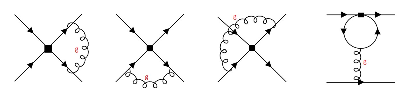
Figure 2: QCD corrections to a four-quark weak process in ${\cal O}(\alpha_{s})$.

In the $Z^{0}$ exchange sector, the following operators mix and form a closed set under such corrections:

$$\begin{split}\Theta_{1}&=[(\bar{u}u)_{V}+(\bar{d}d)_{V}+(\bar{s}s)_{V}]^{\alpha\alpha}[(\bar{u}u)_{A}-(\bar{d}d)_{A}-(\bar{s}s)_{A}]^{\beta\beta}\\ \Theta_{2}&=[(\bar{u}u)_{V}+(\bar{d}d)_{V}+(\bar{s}s)_{V}]^{\alpha\beta}[(\bar{u}u)_{A}-(\bar{d}d)_{A}-(\bar{s}s)_{A}]^{\beta\alpha}\\ \Theta_{3}&=[(\bar{u}u)_{A}+(\bar{d}d)_{A}+(\bar{s}s)_{A}]^{\alpha\alpha}[(\bar{u}u)_{V}-(\bar{d}d)_{V}-(\bar{s}s)_{V}]^{\beta\beta}\\ \Theta_{4}&=[(\bar{u}u)_{A}+(\bar{d}d)_{A}+(\bar{s}s)_{A}]^{\alpha\beta}[(\bar{u}u)_{V}-(\bar{d}d)_{V}-(\bar{s}s)_{V}]^{\beta\alpha}\\ \Theta_{5}&=[(\bar{u}u)_{V}-(\bar{d}d)_{V}-(\bar{s}s)_{V}]^{\alpha\alpha}[(\bar{u}u)_{A}-(\bar{d}d)_{A}-(\bar{s}s)_{A}]^{\beta\beta}\\ \Theta_{6}&=[(\bar{u}u)_{V}-(\bar{d}d)_{V}-(\bar{s}s)_{V}]^{\alpha\beta}[(\bar{u}u)_{A}-(\bar{d}d)_{A}-(\bar{s}s)_{A}]^{\beta\alpha}\\ \Theta_{7}&=[(\bar{u}u)_{A}+(\bar{d}d)_{A}+(\bar{s}s)_{A}]^{\alpha\alpha}[(\bar{u}u)_{V}+(\bar{d}d)_{V}+(\bar{s}s)_{V}]^{\beta\beta}\\ \Theta_{8}&=[(\bar{u}u)_{A}+(\bar{d}d)_{A}+(\bar{s}s)_{A}]^{\alpha\beta}[(\bar{u}u)_{V}+(\bar{d}d)_{V}+(\bar{s}s)_{V}]^{\beta\alpha}\,.\end{split}$$ (4)

The extension to include heavier quarks is made possible by the structure shared by u-like and d-like quarks. For example, once we include all five flavors, $\Theta_{1}$ becomes

$$\Theta_{1}=[(\bar{u}u)_{V}+(\bar{c}c)_{V}+(\bar{d}d)_{V}+(\bar{s}s)_{V}+(\bar{b}b)_{V}]^{\alpha\alpha}[(\bar{u}u)_{A}+(\bar{c}c)_{A}-(\bar{d}d)_{A}-(\bar{s}s)_{A}-(\bar{b}b)_{A}]^{\beta\beta}\,.$$ (5)

Next, using the results from Ref. [14] we calculate the anomalous dimension matrix which represents the QCD mixing of the above operators. This serves as a necessary ingredient in performing a RG analysis:

$$\begin{split}\gamma_{Z}(\mu)&=-\frac{g_{s}^{2}}{8\pi^{2}}\begin{pmatrix}\frac{2}{9}&\frac{-2}{3}&1&-3&0&0&0&0\\ -\frac{3}{2}+\frac{2}{9}n_{f}&\frac{9}{2}-\frac{2}{3}n_{f}&\frac{-3}{2}&\frac{-7}{2}&0&0&0&0\\ \frac{11}{9}&\frac{-11}{3}&0&0&0&0&0&0\\ \frac{-3}{2}&\frac{-7}{2}&\frac{-3}{2}&\frac{9}{2}&0&0&-\frac{2}{9}n_{Q}&\frac{2}{3}n_{Q}\\ 0&0&0&0&1&-3&\frac{2}{9}&-\frac{2}{3}\\ -\frac{2}{9}n_{Q}&\frac{2}{3}n_{Q}&0&0&-3&1&0&0\\ 0&0&0&0&0&0&\frac{11}{9}&-\frac{11}{3}\\ 0&0&0&0&0&0&\frac{2n_{f}}{9}-3&1-\frac{2n_{f}}{3}\\ \end{pmatrix}\,,\end{split}$$ (6)

where $n_{f}$ is the number of dynamical quarks at the considered energy scale and $n_{Q}=n_{d}-n_{u}$, the difference in open $d$-like and $u$-like flavors.

For the $W$ sector, we first consider the u-d current operators that generate and mix in a closed set with

$$\begin{split}&\Theta_{9}=(\bar{u}d)_{V}^{\alpha\alpha}(\bar{d}u)_{A}^{\beta\beta}+(\bar{d}u)_{V}^{\alpha\alpha}(\bar{u}d)_{A}^{\beta\beta}\\ &\Theta_{10}=(\bar{u}d)_{V}^{\alpha\beta}(\bar{d}u)_{A}^{\beta\alpha}+(\bar{d}u)_{V}^{\alpha\beta}(\bar{u}d)_{A}^{\beta\alpha}\\ &\Theta_{ud}^{p_{1}}=[(\bar{u}u)_{V}+(\bar{d}d)_{V}]^{\alpha\alpha}\sum_{q=u,d,s}(\bar{q}q)_{A}^{\beta\beta}+[(\bar{u}u)_{A}+(\bar{d}d)_{A}]^{\alpha\alpha}\sum_{q=u,d,s}(\bar{q}q)_{V}^{\beta\beta}\\ &\Theta_{ud}^{p_{2}}=[(\bar{u}u)_{V}+(\bar{d}d)_{V}]^{\alpha\beta}\sum_{q=u,d,s}(\bar{q}q)_{A}^{\beta\alpha}+[(\bar{u}u)_{A}+(\bar{d}d)_{A}]^{\alpha\beta}\sum_{q=u,d,s}(\bar{q}q)_{V}^{\beta\alpha}\\ &\Theta_{ud}^{p_{3}}=[(\bar{u}u)_{A}+(\bar{d}d)_{A}]^{\alpha\alpha}\sum_{q=u,d,s}(\bar{q}q)_{V}^{\beta\beta}-[(\bar{u}u)_{V}+(\bar{d}d)_{V}]^{\alpha\alpha}\sum_{q=u,d,s}(\bar{q}q)_{A}^{\beta\beta}\\ &\Theta_{ud}^{p_{4}}=[(\bar{u}u)_{A}+(\bar{d}d)_{A}]^{\alpha\beta}\sum_{q=u,d,s}(\bar{q}q)_{V}^{\beta\alpha}-[(\bar{u}u)_{V}+(\bar{d}d)_{V}]^{\alpha\beta}\sum_{q=u,d,s}(\bar{q}q)_{A}^{\beta\alpha}\\ &\Theta_{ud}^{p_{5}}=\sum_{q^{\prime}=u,d,s}\sum_{q=u,d,s}(\bar{q}q)_{A}^{\alpha\alpha}(\bar{q^{\prime}}q^{\prime})_{V}^{\beta\beta}\\ &\Theta_{ud}^{p_{6}}=\sum_{q^{\prime}=u,d,s}\sum_{q=u,d,s}(\bar{q}q)_{A}^{\alpha\beta}(\bar{q^{\prime}}q^{\prime})_{V}^{\beta\alpha}\\ \end{split}$$ (7)

Here, the $\Theta^{p_{i}}_{ud}$ operators are generated by penguin insertions. Noting Ref. [14], the anomalous dimension matrix for the above operators is ultimately found to be

$$\begin{split}\gamma^{ud}_{W}(\mu)&=-\frac{g_{s}^{2}}{8\pi^{2}}\begin{pmatrix}1&-3&0&0&0&0&0&0\\ -3&1&\frac{1}{9}&\frac{-1}{3}&\frac{1}{9}&\frac{-1}{3}&0&0\\ 0&0&\frac{11}{9}&\frac{-11}{3}&\frac{2}{9}&\frac{-2}{3}&0&0\\ 0&0&-3+\frac{n_{f}}{9}&1-\frac{n_{f}}{3}&\frac{n_{f}}{9}&\frac{-n_{f}}{3}&\frac{2}{9}&\frac{-2}{3}\\ 0&0&0&0&-1&3&0&0\\ 0&0&\frac{n_{f}}{9}&\frac{-n_{f}}{3}&\frac{n_{f}}{9}&\frac{n_{f}}{3}-8&\frac{-2}{9}&\frac{2}{3}\\ 0&0&0&0&0&0&\frac{11}{9}&\frac{-11}{3}\\ 0&0&0&0&0&0&\frac{2n_{f}}{9}-3&1-\frac{2n_{f}}{3}\\ \end{pmatrix}\,.\end{split}$$ (8)

The operator set from the u-s current and corresponding anomalous dimension matrix can be found by replacing $d\rightarrow s$. Above the charm-quark mass threshold, the effects of penguin-generated $\Theta^{p_{i}}$ operators of $u$-like quarks cancel each other, as in the $\Delta S=1$ sector [15], due to the Glashow–Iliopoulos–Maiani mechanism, though the analysis below the charm mass scale is richer in the flavor-diagonal case. Nevertheless, the effect of renormalization group flow below the charm-quark mass scale to the hadronic scale of $\mu=2\,\rm GeV$ is negligible compared to the LO evolution of the rest of the operators. Thus, along with the u-s current operators,

$$\begin{split}\Theta_{11}&=(\bar{u}s)_{V}^{\alpha\alpha}(\bar{s}u)_{A}^{\beta\beta}+(\bar{s}u)_{V}^{\alpha\alpha}(\bar{u}s)_{A}^{\beta\beta}\\ \Theta_{12}&=(\bar{u}s)_{V}^{\alpha\beta}(\bar{s}u)_{A}^{\beta\alpha}+(\bar{s}u)_{V}^{\alpha\beta}(\bar{u}s)_{A}^{\beta\alpha}\,,\end{split}$$ (9)

we simplify the anomalous dimension matrix for the $W$ sector as

$$\begin{split}\gamma_{W}(\mu)&=-\frac{g_{s}^{2}}{8\pi^{2}}\begin{pmatrix}1&-3&0&0\\ -3&1&0&0\\ 0&0&1&-3\\ 0&0&-3&1\end{pmatrix}\,.\end{split}$$ (10)

for the set $\Theta_{9},\Theta_{10},\Theta_{11}$, and $\Theta_{12}$. We now turn to our numerical analysis.

3 Renormalization group flow

We start by writing the PV Hamiltonian in Eq. (1) compactly as

$$\mathcal{H}_{\rm eff}^{\rm PV}(\mu)=\frac{G_{F}s_{w}^{2}}{3\sqrt{2}}\sum_{i=1}^{12}C_{i}(\mu)\Theta_{i}\,.$$ (11)

The Wilson coefficients $C_{i}$ flow between different energy scales according to the equation

$$\vec{C}(\mu)=\exp\left[\int_{g_{s}(M_{W})}^{g_{s}(\mu)}dg\frac{\gamma^{T}(\mu)}{\beta(g_{s})}\right]\vec{C}(M_{W})\,.$$ (12)

Here the $\gamma$ matrices from the $W$ and $Z$ sectors are combined as $\gamma=\gamma_{z}\oplus\gamma_{w}$ and the QCD $\beta$ function is

$$\beta(g_{s})=-\frac{g_{s}^{3}}{48\pi^{2}}(33-2n_{f})\,.$$ (13)

As our work is limited to a LO analysis, we use the one-loop expression for the strong-coupling parameter $\alpha_{s}(\mu)=g_{s}^{2}/4\pi$:

$$\alpha_{s}(\mu)=\frac{4\pi}{\beta_{0}\,{\rm ln}(\mu^{2}/\Lambda^{2})}\quad{\rm with}\quad\beta_{0}=\frac{1}{3}(33-2n_{f})\,,$$ (14)

but we have used the two-loop expression for $\alpha_{s}(\mu)$ to set the QCD scale parameters in different energy ranges. With the input value at $Z^{0}$ mass scale, $\alpha_{s}(M_{z})=0.117$ [13], the criterion of continuity across the heavy quark flavor thresholds leads to the following scale parameters: for five-flavor QCD, $\Lambda_{5}=0.214\,\rm GeV$, for four-flavor QCD, $\Lambda_{4}=0.307\,\rm GeV$, and for three-flavor QCD, $\Lambda_{3}=0.352\,\rm GeV$, as this improves the LO analysis considerably. The resulting strong interaction strength ratios at LO [next-to-leading order (NLO)] are

$$\frac{\alpha_{s}(M_{b}=4.18\,\rm GeV)}{\alpha_{s}(M_{W}=80.379\,\rm GeV)}=2.09\,[1.86];\,\frac{\alpha_{s}(M_{c}=1.27\,\rm GeV)}{\alpha_{s}(M_{b})}=1.88\,[1.75];$$

$$\frac{\alpha_{s}(2\,\rm GeV)}{\alpha_{s}(M_{c})}=0.74\,[0.75]\,,$$ (15)

whereas after matching at next-to-next-to-leading order (NNLO), employing the convenient RunDec package [16], the ratios at that order become 1.85, 1.68, and 0.77. Performing the RG flow from the energy scale $M_{W}$ to the hadronic scale of $2\,{\rm GeV}$, $\vec{C}(M_{W})=(1,0,0,0,-3.49,0,0,0,-13.0\cos^{2}\!\theta_{c},0,-13.0\sin^{2}\!\theta_{c},0)$ evolves to

$$\!\!\!\!\!\!\!\!\!\!\vec{C}(2\,\rm GeV)\!=\!\begin{pmatrix}1.09&[1.17\dots 1.06][1.08\dots 1.04]&[1.07][1.06]\\ 0.018&[0.014\dots 0.021][0.033\dots 0.006]&[-0.006][-0.006]\\ 0.199&[0.321\dots 0.133][0.193\dots 0.127]&[0.158][0.153]\\ -0.583&[-0.990\dots-0.385][-0.571\dots-0.374]&[-0.460][-0.456]\\ -4.36&[-4.99\dots-4.05][-4.34\dots-4.03]&[-4.16][-4.14]\\ 1.72&[2.63\dots 1.19][1.67\dots 1.16]&[1.40][1.36]\\ -0.170&[-0.288\dots-0.110][-0.165\dots-0.105]&[-0.134][-0.129]\\ 0.332&[0.496\dots 0.235][0.322\dots 0.225]&[0.275][0.268]\\ -16.2&[-18.6\dots-15.0][-16.1\dots-15.0]&[-15.48][-15.4]\\ 6.38&[9.76\dots 4.44][6.22\dots 4.30]&[5.19][5.05]\\ -16.2&[-18.6\dots-15.0][-16.1\dots-15.0]&[-15.48][-15.4]\\ 6.38&[9.76\dots 4.44][6.22\dots 4.30]&[5.19][5.05]\end{pmatrix}\,,$$ (16)

where the last four entries should be multiplied by factors of $\cos^{2}\!\theta_{c},\cos^{2}\!\theta_{c},\sin^{2}\!\theta_{c}$, and $\sin^{2}\!\theta_{c}$, respectively. Our primary result is given by the leftmost column of numbers, and the coefficients have been simplified with the substitution $s_{W}^{2}=0.231$. The other columns illustrate the uncertainties in our computation. It should be noted that we perform RG-flow below $2\,\rm GeV$ to integrate out the charm quark and then run upwards so as to work with a $N_{f}=2+1$ theory at $2\,\rm GeV$. An alternate would be to evolve to $2\,\rm GeV$ with a $N_{f}=2+1+1$ theory and consider the $u,d,s$ contributions to $H_{\rm eff}$ only. The resulting Wilson coefficients are very similar in the two approaches. In the central column of Eq. (16), the left set shows the ranges of Wilson coefficients that result in the $N_{f}=2+1$ theory for renormalization scales of $\mu=1-4\,{\rm GeV}$ and the right set shows them in the $N_{f}=2+1+1$ theory with $\mu=2-4\,{\rm GeV}$. In the rightmost column, we show the Wilson coefficients if the $\alpha_{s}$ running and matching is computed at NLO (left) and NNLO (right).

We conclude this section by comparing our results with those of Ref. [1], in which the QCD evolution effects were estimated via a phenomenological enhancement factor, $K$:

$$K=1+\frac{g^{2}(\mu^{2})}{16\pi^{2}}\Bigg{(}11-\frac{2}{3}n_{f}\Bigg{)}\,\ln\Bigg{(}\frac{M^{2}_{W}}{\mu^{2}}\Bigg{)}\,,$$ (17)

where $\mu$ is any energy scale below $M_{W}$, $n_{f}$ is the number of dynamical quarks at scale $\mu$, and operator mixing is not included. The Wilson coefficients at hadronic scales corresponding to $K=4$ ($\mu\approx 1.6\,\rm GeV$), after adjusting for an overall sign difference due to differing sign conventions, are found to be $C_{1}^{\rm DDH}=1.15$, $C_{2}^{\rm DDH}=0$, $C_{3}^{\rm DDH}=0$, $C_{4}^{\rm DDH}=-0.39$, $C_{5}^{\rm DDH}=-3.95$,$C_{6}^{\rm DDH}=1.08$, $C_{7}^{\rm DDH}=-0.44$, $C_{8}^{\rm DDH}=1.04$, $C_{9}^{\rm DDH}=-14.67\cos^{2}\!\theta_{c}$, $C_{10}^{\rm DDH}=4.02\cos^{2}\!\theta_{c}$, $C_{11}^{\rm DDH}=-14.67\sin^{2}\!\theta_{c}$ and $C_{12}^{\rm DDH}=4.02\sin^{2}\!\theta_{c}$. Comparing to Eq. (16), we observe that the QCD operator mixing and flavor threshold effects necessary for a complete calculation play an important numerical role, with earlier results [1] falling outside the range possible through the consideration of scale variation and higher-order effects.

4 Isosector extractions

With the full PV effective Hamiltonian in hand, we extract the contributions from the individual isosectors. For example, for the isovector sector:

$$\mathcal{H}_{\rm eff}^{\rm PV}(\mu)=\frac{G_{F}s_{w}^{2}}{3\sqrt{2}}\sum_{i=1}^{12}C_{i}(\mu)\Theta_{i}\longrightarrow\mathcal{H}^{I=1}_{\rm eff}(\mu)=\frac{G_{F}s_{w}^{2}}{3\sqrt{2}}\sum_{i=1}^{12}C^{I=1}_{i}(\mu)\Theta_{i}^{I=1}$$ (18)

Considering the operators in Eqs.(4, 7, 9) we see $\Theta_{1-4,11,12}$ contribute one operator each: $C_{j}\Theta_{j}\rightarrow C^{I=1}_{j}\Theta^{I=1}_{j}$ with $C_{j}=C^{I=1}_{j}$. Operators $\Theta_{5}$ and $\Theta_{6}$ contribute two operators each: $C_{5}\Theta_{5}\rightarrow C^{I=1}_{5}\Theta_{5}^{I=1}+C^{I=1}_{7}\Theta_{7}^{I=1}$ with $C^{I=1}_{5}=C^{I=1}_{7}=-C_{5}$ and $C_{6}\Theta_{6}\rightarrow C^{I=1}_{6}\Theta_{6}^{I=1}+C^{I=1}_{8}\Theta_{8}^{I=1}$ with $C^{I=1}_{6}=C^{I=1}_{8}=-C_{6}$. Operators $\Theta_{7-10}$ have no contributions to the isovector sector. Thus the extracted isovector operator set is

$$\begin{split}\Theta_{1}&{}^{I=1}=[(\bar{u}u)_{V}+(\bar{d}d)_{V}+(\bar{s}s)_{V}]^{\alpha\alpha}[(\bar{u}u)_{A}-(\bar{d}d)_{A}]^{\beta\beta}\\ \Theta_{2}&{}^{I=1}=[(\bar{u}u)_{V}+(\bar{d}d)_{V}+(\bar{s}s)_{V}]^{\alpha\beta}[(\bar{u}u)_{A}-(\bar{d}d)_{A}]^{\beta\alpha}\\ \Theta_{3}&{}^{I=1}=[(\bar{u}u)_{A}+(\bar{d}d)_{A}+(\bar{s}s)_{A}]^{\alpha\alpha}[(\bar{u}u)_{V}-(\bar{d}d)_{V}]^{\beta\beta}\\ \Theta_{4}&{}^{I=1}=[(\bar{u}u)_{A}+(\bar{d}d)_{A}+(\bar{s}s)_{A}]^{\alpha\beta}[(\bar{u}u)_{V}-(\bar{d}d)_{V}]^{\beta\alpha}\\ \Theta_{5}&{}^{I=1}=(\bar{s}s)_{V}^{\alpha\alpha}[(\bar{u}u)_{A}-(\bar{d}d)_{A}]^{\beta\beta}\\ \Theta_{6}&{}^{I=1}=(\bar{s}s)_{V}^{\alpha\beta}[(\bar{u}u)_{A}-(\bar{d}d)_{A}]^{\beta\alpha}\\ \Theta_{7}&{}^{I=1}=(\bar{s}s)_{A}^{\alpha\alpha}[(\bar{u}u)_{V}-(\bar{d}d)_{V}]^{\beta\beta}\\ \Theta_{8}&{}^{I=1}=(\bar{s}s)_{A}^{\alpha\beta}[(\bar{u}u)_{V}-(\bar{d}d)_{V}]^{\beta\alpha}\\ \Theta_{9}&{}^{I=1}=(\bar{u}s)_{V}^{\alpha\alpha}(\bar{s}u)_{A}^{\beta\beta}+(\bar{s}u)_{V}^{\alpha\alpha}(\bar{u}s)_{A}^{\beta\beta}\\ \Theta_{10}&{}^{I=1}=(\bar{u}s)_{V}^{\alpha\beta}(\bar{s}u)_{A}^{\beta\alpha}+(\bar{s}u)_{V}^{\alpha\beta}(\bar{u}s)_{A}^{\beta\alpha}\\ \end{split}\,,$$ (19)

and the extracted isovector Wilson coefficients at high and low energies are: $\vec{C}^{I=1}(M_{W})=(1,0,0,0,3.49,0,3.49,0,-13.0\cos^{2}\!\theta_{c},0)$ and

$$\!\!\!\!\!\!\!\!\!\!\vec{C}^{I=1}(2\,\rm GeV)\!=\!\begin{pmatrix}1.09&[1.17\dots 1.06][1.08\dots 1.04]&[1.07][1.06]\\ 0.018&[0.014\dots 0.021][0.033\dots 0.006]&[-0.006][-0.006]\\ 0.199&[0.321\dots 0.133][0.193\dots 0.127]&[0.158][0.153]\\ -0.583&[-0.990\dots-0.385][-0.571\dots-0.374]&[-0.460][-0.456]\\ 4.36&[4.99\dots 4.05][4.34\dots 4.03]&[4.16][4.14]\\ -1.72&[-2.63\dots-1.19][-1.67\dots-1.16]&[-1.40][-1.36]\\ 4.36&[4.99\dots 4.05][4.34\dots 4.03]&[4.16][4.14]\\ -1.72&[-2.63\dots-1.19][-1.67\dots-1.16]&[-1.40][-1.36]\\ -16.2&[-18.6\dots-15.0][-16.1\dots-15.0]&[-15.48][-15.4]\\ 6.38&[9.76\dots 4.44][6.22\dots 4.30]&[5.19][5.05]\\ \end{pmatrix}\,,$$ (20)

where the last two entries should be multiplied by a factor $\sin^{2}\!\theta_{c}$ and the error estimates are defined as in Eq. (16). Alternatively, an isovector RG analysis can be performed directly to get $\vec{C}^{I=1}(2\,\rm GeV)$ from $\vec{C}^{I=1}(M_{W})$ using the anomalous dimension matrix corresponding to the operator set in Eq.(19):

$$\begin{split}\gamma_{Z}^{I=1}&=-\frac{g_{s}}{8\pi^{2}}\begin{pmatrix}\frac{2}{9}&\frac{-2}{3}&1&-3&0&0&0&0\\ -\frac{3}{2}+\frac{2}{9}n_{f}&\frac{9}{2}-\frac{2}{3}n_{f}&\frac{-3}{2}&\frac{-7}{2}&0&0&0&0\\ \frac{11}{9}&\frac{-11}{3}&0&0&0&0&0&0\\ \frac{-3}{2}&\frac{-7}{2}&\frac{-3}{2}&\frac{9}{2}&0&0&0&0\\ 0&0&0&0&0&0&1&-3\\ \frac{2}{9}n_{Q}&-\frac{2}{3}n_{Q}&0&0&\frac{-3}{2}&\frac{9}{2}&\frac{-3}{2}&\frac{-7}{2}\\ 0&0&0&0&1&-3&0&0\\ 0&0&0&0&\frac{-3}{2}&\frac{-7}{2}&\frac{-3}{2}&\frac{9}{2}\\ \end{pmatrix}\end{split}$$ (21)

The corresponding $W$ sector matrix can be easily obtained from Eq. (10). The set of Wilson coefficients obtained via RG flow exactly matches the results in Eq. (20), in agreement with Fig. (1). A purely isovector $Z^{0}$ sector RG analysis was performed in Ref. [10]. Our results are in agreement when the same inputs are used.

We can make a similar analysis in the $I=0\oplus 2$ sector. The corresponding operators are

$$\begin{split}\Theta_{1}&{}^{I=0\oplus 2}=[(\bar{u}u)_{V}+(\bar{d}d)_{V}+(\bar{s}s)_{V}]^{\alpha\alpha}[(\bar{s}s)_{A}]^{\beta\beta}\\ \Theta_{2}&{}^{I=0\oplus 2}=[(\bar{u}u)_{V}+(\bar{d}d)_{V}+(\bar{s}s)_{V}]^{\alpha\beta}[(\bar{s}s)_{A}]^{\beta\alpha}\\ \Theta_{3}&{}^{I=0\oplus 2}=[(\bar{u}u)_{A}+(\bar{d}d)_{A}+(\bar{s}s)_{A}]^{\alpha\alpha}[(\bar{s}s)_{V}]^{\beta\beta}\\ \Theta_{4}&{}^{I=0\oplus 2}=[(\bar{u}u)_{A}+(\bar{d}d)_{A}+(\bar{s}s)_{A}]^{\alpha\beta}[(\bar{s}s)_{V}]^{\beta\alpha}\\ \Theta_{5}&{}^{I=0\oplus 2}=[(\bar{u}u)_{V}-(\bar{d}d)_{V}]^{\alpha\alpha}[(\bar{u}u)_{A}-(\bar{d}d)_{A}]^{\beta\beta}+(\bar{s}s)_{V}^{\alpha\alpha}(\bar{s}s)_{A}^{\beta\beta}\\ \Theta_{6}&{}^{I=0\oplus 2}=[(\bar{u}u)_{V}-(\bar{d}d)_{V}]^{\alpha\beta}[(\bar{u}u)_{A}-(\bar{d}d)_{A}]^{\beta\alpha}+(\bar{s}s)_{V}^{\alpha\beta}(\bar{s}s)_{A}^{\beta\alpha}\\ \Theta_{7}&{}^{I=0\oplus 2}=[(\bar{u}u)_{V}+(\bar{d}d)_{V}+(\bar{s}s)_{V}]^{\alpha\alpha}[(\bar{u}u)_{A}+(\bar{d}d)_{A}+(\bar{s}s)_{A}]^{\beta\beta}\\ \Theta_{8}&{}^{I=0\oplus 2}=[(\bar{u}u)_{A}+(\bar{d}d)_{A}+(\bar{s}s)_{A}]^{\alpha\beta}[(\bar{u}u)_{V}+(\bar{d}d)_{V}+(\bar{s}s)_{V}]^{\beta\alpha}\\ \Theta_{9}&{}^{I=0\oplus 2}=(\bar{u}d)_{V}^{\alpha\alpha}(\bar{d}u)_{A}^{\beta\beta}+(\bar{d}u)_{V}^{\alpha\alpha}(\bar{u}d)_{A}^{\beta\beta}\\ \Theta_{10}&{}^{I=0\oplus 2}=(\bar{u}d)_{V}^{\alpha\beta}(\bar{d}u)_{A}^{\beta\alpha}+(\bar{d}u)_{V}^{\alpha\beta}(\bar{u}d)_{A}^{\beta\alpha}\\ \end{split}\,,$$ (22)

and the extracted Wilson coefficients for the $I=0\oplus 2$ sector at high and low energies are: $\vec{C}^{I=0\oplus 2}(M_{W})=(-1,0,0,0,-3.49,0,0,0,-13.0\cos^{2}\!\theta_{c},0)$ and

$$\!\!\!\!\!\!\!\!\!\!\vec{C}^{I=0\oplus 2}(2\,\rm GeV)\!=\!\begin{pmatrix}-1.09&[-1.17\dots-1.06][-1.08\dots-1.04]&[-1.07][-1.06]\\ -0.018&[-0.014\dots-0.021][-0.033\dots-0.006]&[0.006][0.006]\\ -0.199&[-0.321\dots-0.133][-0.193\dots-0.127]&[-0.158][-0.153]\\ 0.583&[0.990\dots 0.385][0.571\dots 0.374]&[0.460][0.456]\\ -4.36&[-4.99\dots-4.05][-4.34\dots-4.03]&[-4.16][-4.14]\\ 1.72&[2.63\dots 1.19][1.67\dots 1.16]&[1.40][1.36]\\ -0.170&[-0.288\dots-0.110][-0.165\dots-0.105]&[-0.134][-0.129]\\ 0.332&[0.496\dots 0.235][0.322\dots 0.225]&[0.275][0.268]\\ -16.2&[-18.6\dots-15.0][-16.1\dots-15.0]&[-15.48][-15.4]\\ 6.38&[9.76\dots 4.44][6.22\dots 4.30]&[5.19][5.05]\\ \end{pmatrix}$$ (23)

where the last two entries should be multiplied by a factor $\cos^{2}\!\theta_{c}$ and the error estimates are defined as in Eq. (16). If one wishes to perform a RG analysis of the isoeven sectors to obtain $\vec{C}^{I=0\oplus 2}(2\,\rm GeV)$ from $\vec{C}^{I=0\oplus 2}(M_{W})$, the anomalous dimension matrix for the operator set in Eq.(22) is

$$\begin{split}\gamma^{I=0\oplus 2}_{Z}&=-\frac{g_{s}}{8\pi^{2}}\begin{pmatrix}\frac{2}{9}&\frac{-2}{3}&1&-3&0&0&0&0\\ -\frac{3}{2}+\frac{2}{9}n_{f}&\frac{9}{2}-\frac{2}{3}n_{f}&\frac{-3}{2}&\frac{-7}{2}&0&0&0&0\\ \frac{11}{9}&\frac{-11}{3}&0&0&0&0&0&0\\ \frac{-3}{2}&\frac{-7}{2}&\frac{-3}{2}&\frac{9}{2}&0&0&\frac{2}{9}n_{Q}&-\frac{2}{3}n_{Q}\\ 0&0&0&0&1&-3&\frac{2}{9}&-\frac{2}{3}\\ \frac{2}{9}n_{Q}&-\frac{2}{3}n_{Q}&0&0&-3&1&0&0\\ 0&0&0&0&0&0&\frac{11}{9}&-\frac{11}{3}\\ 0&0&0&0&0&0&\frac{2n_{f}}{9}-3&1-\frac{2n_{f}}{3}\\ \end{pmatrix}\end{split}\,,$$ (24)

and the $W$ sector matrix can be easily obtained from Eq. (10). Again, the set of Wilson coefficients obtained via RG flow exactly matches the extracted coefficients sets in Eq. (23), in agreement with Fig. (1).

5 Estimation of the parity-violating pion-NN coupling constant

We can now use our effective Hamiltonian to compute the parity-violating meson-NN coupling constants of isospin $I$, $h_{M}^{I}$, that appear in the phenomenological Hamiltonian $\mathcal{H}_{\rm DDH}$ [1], to compare and contrast with earlier estimates. For example, the one-pion contribution to hadronic parity violation stems from

$$\mathcal{H}^{\pi}_{\rm DDH}=ih^{1}_{\pi}(\pi^{+}\bar{p}n-\pi^{-}\bar{n}p)\,,$$ (25)

implying that $h_{\pi}^{1}$ can be determined via

$$-ih_{\pi}^{1}\bar{u}_{n}u_{p}=\bra{n\pi^{+}}\mathcal{H}_{\rm eff}^{I=1}\ket{p}\,,$$ (26)

where $u_{N}$ with $N\in p,n$ is a Dirac spinor. Using the factorization approximation [17, 18] on the matrix element of Eq. (26), we have

$$h_{\pi}^{1}\bar{u}_{n}u_{p}=\frac{2G_{F}s_{w}^{2}}{3\sqrt{2}}\left(\frac{C_{1}^{I=1}}{N_{c}}+C_{2}^{I=1}-\frac{C_{3}^{I=1}}{N_{c}}-C_{4}^{I=1}\right)\frac{m_{\pi}^{2}f_{\pi}}{(m_{u}+m_{d})}\bra{n}\bar{d}u\ket{p}\,,$$ (27)

where $N_{c}=3$ and we have simplified our result using the quark-field equations of motion and $\langle 0|(\bar{d}u)_{A}(0)|\pi^{+}(p)\rangle\equiv ip^{\mu}f_{\pi}$ to find

$$\bra{\pi^{+}}(\bar{u}\gamma_{5}d)\ket{0}=\frac{m_{\pi}^{2}f_{\pi}}{i(m_{u}+m_{d})}\,.$$ (28)

For the numerical evaluation of Eq. (27) we use $m_{\pi}=135\,\rm MeV$ and the charged-pion decay constant $f_{\pi}=130\,\rm MeV$, with the other inputs coming from $N_{f}=2+1$ lattice QCD (LQCD) results: the renormalization-group-invariant (RGI) mass $(m_{u}+m_{d})=2(4.695(56)_{m}(54)_{\Lambda}\,\rm MeV)$  [19] and the isovector quark scalar charge of the nucleon ($\bra{n}\bar{d}u\ket{p}\equiv g_{s}^{u-d}\bar{u}_{n}u_{p}$) with $g_{s}^{u-d}=1.06(10)(06)_{sys}$ [20] at $\mu=2\,{\rm GeV}$. Using Eq. (20) we find

$$h_{\pi}^{1}=(3.06\pm 0.34+\left(\stackrel{{\scriptstyle{+1.29}}}{{{}_{-0.64}}}\right)+0.42+(1.00))\times 10^{-7}\,,$$ (29)

where the error estimates come, respectively, from the LQCD inputs we employ and from the following systematic effects: the change in the Wilson coefficients over (i) a scale variation of $1-4\,{\rm GeV}$ and (ii) higher-order corrections in $\alpha_{s}$ as per Eq. (20), and, finally, our estimate of the accuracy of Eq. (27) through the contribution to it from ${\cal O}(1/N_{c})$ terms, which we note in parentheses. We emphasize that this last could be an underestimate of the uncertainty. To compare, the DDH “best value” of $h_{\pi}^{1}=4.6\times 10^{-7}$ [1] neglects operator mixing as noted after Eq.(17), although that value is driven by their estimate of non-factorizable contributions, which may be grossly overestimated [8]. A computation with Wilson coefficients compatible with ours yields $h_{\pi}^{1}\sim 1.5\times 10^{-7}$ at $\mu=1\,{\rm GeV}$ using the factorization approximation, a SU(3)_f-based assumption for the nucleon matrix element, and phenomenological fits for the light quark mass ratios with $m_{s}=200\,{\rm MeV}$ — but $h_{\pi}^{1}\sim 6\times 10^{-7}$ using SU(3)_f transformations and hyperon data [11], trends also noted in two- and three-flavor Skyrme models [21, 22], albeit their outcomes are much smaller. These large variations in $h_{\pi}^{1}$ are remediated through the use of LQCD for the nucleon matrix element. The experimental result $h_{\pi}^{1}=2.6(1.2)_{\rm stat}(0.2)_{\rm sys}\times 10^{-7}$, determined from the parity-violating gamma asymmetry in ${\vec{n}}p\to d\gamma$ [5], is also comparable to its value extracted using chiral EFT [23, 24], and we believe our improved comparison to it affirms the validity of our approach. We refer to Ref. [25] for further discussion and broader examples.

6 Summary

We have determined the effective weak Hamiltonian for parity-violating, $\Delta S=0$ hadronic processes in the Standard Model at a renormalization scale of $2\,\rm GeV$. To do this, we have made a complete, LO renormalization group analysis in QCD, starting from just below the $W$ mass scale, including operator mixing and evolution through heavy-flavor thresholds, as well as neutral- and charged-current effects, for all possible isospins ($I=0,1,2$) of the four-quark operators. In our analysis we have found it convenient to separate the $I=1$ and $I=0\oplus 2$ sectors, and isospin symmetry allows us to recover the same low-energy effective Hamiltonian regardless of the order in which we (i) evolve to low-energy scales or (ii) project on operators with even or odd isospin — a test, which we note here for the first time, that should prove particularly useful in a future NLO analysis. The construction of the complete effective weak Hamiltonian at a scale of $\mu=2\,\rm GeV$ should support LQCD studies of two-nucleon matrix elements [26], enabling further theoretical studies in which the factorization approximation of the hadronic matrix elements would finally be no longer necessary.

References

• [1] B. Desplanques, J. F. Donoghue, B. R. Holstein, Unified Treatment of the Parity Violating Nuclear Force, Annals Phys. 124 (1980) 449. doi:10.1016/0003-4916(80)90217-1.
• [2] D. R. Phillips, D. Samart, C. Schat, Parity-Violating Nucleon-Nucleon Force in the 1/$N_{c}$ Expansion, Phys. Rev. Lett. 114 (6) (2015) 062301. arXiv:1410.1157, doi:10.1103/PhysRevLett.114.062301.
• [3] M. R. Schindler, R. P. Springer, J. Vanasse, Large-$N_{c}$ limit reduces the number of independent few-body parity-violating low-energy constants in pionless effective field theory, Phys. Rev. C 93 (2) (2016) 025502, [Erratum: Phys.Rev.C 97, 059901 (2018)]. arXiv:1510.07598, doi:10.1103/PhysRevC.93.025502.
• [4] S. Gardner, W. C. Haxton, B. R. Holstein, A New Paradigm for Hadronic Parity Nonconservation and its Experimental Implications, Ann. Rev. Nucl. Part. Sci. 67 (2017) 69–95. arXiv:1704.02617, doi:10.1146/annurev-nucl-041917-033231.
• [5] D. Blyth, et al., First Observation of $P$-odd $\gamma$ Asymmetry in Polarized Neutron Capture on Hydrogen, Phys. Rev. Lett. 121 (24) (2018) 242002. arXiv:1807.10192, doi:10.1103/PhysRevLett.121.242002.
• [6] M. T. Gericke, et al., First Precision Measurement of the Parity Violating Asymmetry in Cold Neutron Capture on 3He, Phys. Rev. Lett. 125 (13) (2020) 131803. arXiv:2004.11535, doi:10.1103/PhysRevLett.125.131803.
• [7] S.-L. Zhu, Large ${N}_{c}$ expansion and the parity-violating $\pi$, $n$, $\Delta$ couplings, Phys. Rev. D 79 (2009) 116002. doi:10.1103/PhysRevD.79.116002.
• [8] V. M. Dubovik, S. V. Zenkin, Formation of parity nonconserving nuclear forces in the standard model SU(2)(l) X U(1) X SU(3)(c), Annals Phys. 172 (1986) 100–135. doi:10.1016/0003-4916(86)90021-7.
• [9] B. Tiburzi, Isotensor hadronic parity violation, Phys. Rev. D86 (2012) 097501. arXiv:1207.4996, doi:10.1103/PhysRevD.86.097501.
• [10] J. Dai, M. J. Savage, J. Liu, R. P. Springer, Low-energy effective Hamiltonian for Delta I = 1 nuclear parity violation and nucleonic strangeness, Phys. Lett. B 271 (1991) 403–409. doi:10.1016/0370-2693(91)90108-3.
• [11] D. B. Kaplan, M. J. Savage, An analysis of parity-violating pion-nucleon couplings, Nuclear Physics A 556 (4) (1993) 653–671.
• [12] B. Tiburzi, Hadronic parity violation at next-to-leading order, Phys. Rev. D85 (2012) 054020. arXiv:1201.4852, doi:10.1103/PhysRevD.85.054020.
• [13] P. A. Zyla, et al., Review of Particle Physics, PTEP 2020 (8) (2020) 083C01. doi:10.1093/ptep/ptaa104.
• [14] R. D. C. Miller, B. H. J. McKellar, Anomalous-dimension matrices of four-quark operators, Phys. Rev. D 28 (4) (1983) 844–855. doi:10.1103/PhysRevD.28.844.
• [15] G. Buchalla, A. J. Buras, M. E. Lautenbacher, Weak decays beyond leading logarithms, Rev. Mod. Phys. 68 (1996) 1125–1144. arXiv:hep-ph/9512380, doi:10.1103/RevModPhys.68.1125.
• [16] K. G. Chetyrkin, J. H. Kuhn, M. Steinhauser, RunDec: A Mathematica package for running and decoupling of the strong coupling and quark masses, Comput. Phys. Commun. 133 (2000) 43–65. arXiv:hep-ph/0004189, doi:10.1016/S0010-4655(00)00155-7.
• [17] F. C. Michel, Parity Nonconservation in Nuclei, Phys. Rev. 133 (1964) B329–B349. doi:10.1103/PhysRev.133.B329.
• [18] M. Bauer, B. Stech, M. Wirbel, Exclusive Nonleptonic Decays of D, D(s), and B Mesons, Z. Phys. C 34 (1987) 103. doi:10.1007/BF01561122.
• [19] Y. Aoki, et al., FLAG Review 2021 (11 2021). arXiv:2111.09849.
• [20] S. Park, R. Gupta, B. Yoon, S. Mondal, T. Bhattacharya, Y.-C. Jang, B. Joó, F. Winter, Precision nucleon charges and form factors using (2+1)-flavor lattice QCD, Phys. Rev. D 105 (5) (2022) 054505. arXiv:2103.05599, doi:10.1103/PhysRevD.105.054505.
• [21] N. Kaiser, U. G. Meissner, The Weak Pion - Nucleon Vertex Revisited, Nucl. Phys. A 489 (1988) 671–682. doi:10.1016/0375-9474(88)90115-7.
• [22] U. G. Meissner, H. Weigel, The Parity violating pion nucleon coupling constant from a realistic three flavor Skyrme model, Phys. Lett. B 447 (1999) 1–7. arXiv:nucl-th/9807038, doi:10.1016/S0370-2693(98)01569-X.
• [23] J. de Vries, N. Li, U.-G. Meißner, A. Nogga, E. Epelbaum, N. Kaiser, Parity violation in neutron capture on the proton: Determining the weak pion–nucleon coupling, Phys. Lett. B 747 (2015) 299–304. arXiv:1501.01832, doi:10.1016/j.physletb.2015.05.074.
• [24] J. de Vries, E. Epelbaum, L. Girlanda, A. Gnech, E. Mereghetti, M. Viviani, Parity- and time-reversal-violating nuclear forces, Front. in Phys. 8 (2020) 218. arXiv:2001.09050, doi:10.3389/fphy.2020.00218.
• [25] S. Gardner, G. Muralidhara, QCD Analysis of $\Delta S=0$ Hadronic Parity Violation (2022). arXiv:2203.00033v1.
• [26] A. Nicholson, et al., Toward a resolution of the NN controversy, in: 38th International Symposium on Lattice Field Theory, 2021. arXiv:2112.04569.