Massive central galaxies of galaxy groups in the Romulus simulations: an overview of galaxy properties at $z=0$

Abstract

Contrary to many stereotypes about massive galaxies, observed brightest group galaxies (BGGs) are diverse in their star formation rates, kinematic properties, and morphologies. Studying how they evolve into and express such diverse characteristics is an important piece of the galaxy formation puzzle. We use a high-resolution cosmological suite of simulations Romulus and compare simulated central galaxies in group-scale halos at $z=0$ to observed BGGs. The comparison encompasses the stellar mass-halo mass relation, various kinematic properties and scaling relations, morphologies, and the star formation rates. Generally, we find that Romulus reproduces the full spectrum of diversity in the properties of the BGGs very well, albeit with a tendency toward lower than the observed fraction of quenched BGGs. We find both early-type S0 and elliptical galaxies as well as late-type disk galaxies; we find Romulus galaxies that are fast-rotators as well as slow-rotators; and we observe galaxies transforming from late-type to early-type following strong dynamical interactions with satellites. We also carry out case studies of selected Romulus galaxies to explore the link between their properties, and the recent evolution of the stellar system as well as the surrounding intragroup/circumgalactic medium. In general, mergers/strong interactions quench star-forming activity and disrupt the stellar disk structure. Sometimes, however, such interactions can also trigger star-formation and galaxy rejuvenation. Black hole feedback can also lead to a decline of the star formation rate but by itself, it does not typically lead to complete quenching of the star formation activity in the BGGs.

1 Introduction

Massive galaxies sit at the apex of the hierarchy of galaxies. Often found in galaxy groups and clusters, and typically close to the bottom of the gravitational potential wells of their host systems, these galaxies are the most luminous and the most massive galaxies in the present-day Universe. Observational studies find that many of the properties of massive central galaxies, including the Brightest Cluster galaxies (BCGs) and the Brightest Group galaxies (BGGs), bear the imprint of the unique environment in which they reside (e.g., Von Der Linden et al. 2007; Liu et al. 2008a; Yoon et al. 2017).

Early analytic models of the evolution of galaxy groups and clusters (see, for example, Balogh et al., 1999; Babul et al., 2002), however paid little attention to the evolution of the central galaxies in these systems, focusing instead on the emergence and the evolution of the intragroup/intracluster gas (hereafter, IGrM and ICM, respectively). Even the assessment of contemporary numerical models galaxy groups and clusters has tended to focus on the properties of the IGrM/ICM (see, for example, Davé et al., 2008; McCarthy et al., 2010; Le Brun et al., 2014; Schaye et al., 2015; Liang et al., 2016; Barnes et al., 2017; Henden et al., 2018; Robson & Davé, 2020, and references therein). We suggest that the observed properties of the BGGs & BCGs  and the existence of correlations between these and the properties of the host systems offer an equally powerful, complementary way to assess the reliability of theoretical and numerical models. In fact, these trends indicate that the evolution of the BGGs & BCGs  and that of their host groups and clusters are so intimately intertwined that the study of the BGGs & BCGs  offers an alternative window into the physical processes that drive the evolution of the groups and clusters.

In observations, the most frequently discussed BGG & BCG  properties are their stellar masses, sizes and surface brightness profiles, all of which exhibit strong correlations with properties of the host group/cluster (Brough et al., 2005, 2008; Zhao et al., 2015b; Kravtsov et al., 2018; Furnell et al., 2018). Various studies show that the galaxies’ morphological (Zhao et al., 2015b; Cougo et al., 2020) and structural properties (Zhao et al., 2015a) as well as star formation rates (Gozaliasl et al., 2016) are also correlated with the host halo mass. These latter findings complement and reinforce previous results of Weinmann et al. (2006, hereafter W06) who found a clear linear relationship between the fraction of central galaxies that are early- and late-types, and the host halo mass: the late-type fraction (i.e., the fraction of central galaxies that are blue and actively star forming) decreases with increasing halo mass from $\sim 0.6$ at $M_{\rm halo}=10^{12}\,h^{-1}\,\rm M_{\odot}$ to $<0.2$ at $M_{\rm halo}>10^{14}\,h^{-1}\,\rm M_{\odot}$ while the early-type fraction (i.e., the fraction of central galaxies that are red and host little or no on-going star formation) increases with increasing halo mass from $\sim 0.2$ at $M_{\rm halo}=10^{12}\,h^{-1}\,\rm M_{\odot}$ to ${\;\raise 1.29167pt\hbox{$>$\kern-7.5pt\raise-4.73611pt\hbox{$\sim$}}\;}0.6$ at $M_{\rm halo}>10^{14}\,h^{-1}\,\rm M_{\odot}$.

Similarly, the observed kinematic properties of these galaxies also vary considerably with halo mass. Loubser et al. (2018, hereafter L18) show that the radial stellar velocity dispersion profile of typical BGGs in low mass groups decreases with radius while that of most BCGs rises with radius. L18 also find a significant difference between BGGs’ and BCGs’ anisotropy parameter ($V_{\rm max}/\sigma_{0}$), which quantifies the global dynamical importance of rotational and random motions of stars in a galaxy. Typically, BGGs in low mass groups have a higher anisotropy parameter ($V_{\rm max}/\sigma_{0}{\;\raise 1.29167pt\hbox{$>$\kern-7.5pt\raise-4.73611pt\hbox{$\sim$}}\;}0.6$) than BCGs in massive clusters ($V_{\rm max}/\sigma_{0}\approx 0.1$). In other words, the probability that a central galaxy is a fast or a slow rotator depends strongly on the mass of host halo. A similar mass dependency is found in the kinematic spheroid-to-total ratio (S/T). Modeling 3D stellar obital distributions of central galaxies from the CALIFA survey, Zhu et al. (2018) show that the contribution of cold orbits (i.e., the rotating component) to the total decreases with growing system mass.

These observed halo mass dependent trends indicate that the present-day BGGs & BCGs  are not self-similar systems. Even if BCGs themselves were once BGGs at an earlier epoch of their evolution, over time they inevitably express distinct properties by virtue of the fact that they have evolved in much deeper gravitational potential wells that are characterized by much higher virial velocities and temperatures, and likely have been shaped by many more mergers/interactions than present-day BGGs.

A number of studies, including Schaye et al. (2015), Dubois et al. (2016), Clauwens et al. (2018), Davé et al. (2019), Tacchella et al. (2019), Davison et al. (2020), and Pulsoni et al. (2020); Pulsoni et al. (2021), have reported on the properties of central galaxies in their simulations. While their samples do include BGGs, these studies are mainly interested in trends across a broad spectrum of galaxies spanning 2 to 3 orders of magnitude in stellar mass. Only a handful of investigations have focused specifically on the evolution of BGGs  (Ragone-Figueroa et al. 2013; Ragone-Figueroa et al. 2018; Ragone-Figueroa et al. 2020; Le Brun et al. 2014, Martizzi et al. 2014; Remus et al. 2017, Nipoti 2017; Pillepich et al. 2018, Rennehan et al. 2020; Jackson et al. 2020; Henden et al. 2020; Bassini et al. 2020; Marini et al. 2021; see also Section 4 of recent review article by Oppenheimer et al. 2021.). In this paper, we examine the properties and the evolution of a population of BGGs from the Romulus suite of simulations.

The Romulus suite consists of a set of four smooth particle hydrodynamic (SPH) cosmological simulations, Romulus25, RomulusC, RomulusG1 and RomulusG2, all of which were run using the Tree+SPH code CHaNGa (Menon et al., 2015) and have the same hydrodynamics, sub-grid physics, resolution and background cosmology. Among the defining features of the Romulus simulations is their resolution. With dark matter particle mass of $3.39\times 10^{5}\,\rm M_{\rm\odot}$, gas particle mass of $2.12\times 10^{5}\,\rm M_{\rm\odot}$, a Plummer equivalent gravitational force softening of $250\,{\rm pc}$, and maximum SPH resolution of $70\,{\rm pc}$ (Tremmel et al., 2017, 2019), the simulations rank among the highest resolution cosmological simulations run to $z=0$. Of the four simulations in the suite, three are zoom-in simulations of individual systems — RomulusG1 and RomulusG2 are zoom-in simulations of two bona fide galaxy groups and RomulusC is a zoom-in simulation of a massive group/low-mass cluster (Tremmel et al., 2019; Chadayammuri et al., 2021) — while Romulus25 is a simulation of a cosmological volume corresponding to a periodic cube with length $25\,{\rm Mpc}$ per side. Together, these four simulations result in the sample of 19 massive halos in the mass range of interest to us (described further in Section 2.2). We assess their properties, compare these against observations, and seek insights into how these properties arise. We also occasionally compute and juxtapose the corresponding properties of central galaxies in slightly lower mass halos for comparison. Tremmel et al. (2017) have shown that the properties of these lower mass galaxies in Romulus are in good agreement with observations.

This is the first of the series of papers exploring the evolution of massive central galaxies in Romulus suite. This paper is structured as follows: We briefly describe the Romulus simulations and the BGGs sample that we extract from these simulations in Section 2. In Section 3, we describe the various properties and scaling relations that the Romulus BGGs exhibit, and compare these to observational as well as other simulation results. This includes the stellar mass-halo mass relation, stellar kinematics, morphology, and star formation rates. Section 4 offers an examination of how these properties arise. The conclusion and summary is presented in Section 5.

2 Methods

2.1 A brief overview of the Romulus simulations

Table 1: The number of BGGs extracted from the individual simulations used in this study, and their host halo masses.

		Number of halos	Number of halos
Simulation	$M_{\rm 200}$ [M⊙]	($M_{\rm 200}/M_{\odot}\geq 10^{12.5}$)	($10^{12}\leq M_{\rm 200}/M_{\odot}<10^{12.5}$)
RomulusC	$1.15\times 10^{14}$	1	–
RomulusG1	$1.58\times 10^{13}$	1	–
RomulusG2	$4.27\times 10^{13}$	1	–
Romulus25	$[1.19\times 10^{12},1.73\times 10^{13}]$	16	19

A detailed description of the Romulus simulations, including a thorough exposition of the code used to run the individual simulations and the details about the sub-grid physics used, appear in a number of papers. We refer interested readers to the following: Menon et al. (2015), Wadsley et al. (2017), and Tremmel et al. (2015); Tremmel et al. (2017, 2019). The following is a very brief summary.

The CHaNGa code used to run the Romulus simulations utilizes many of the sub-grid physics models that have been previously implemented in the simulation code GASOLINE/GASOLINE2 and extensively tested (Stinson et al. 2006). These include modules handling star formation, stellar feedback, turbulent diffusion (Shen et al. 2010), the UV background with self-shielding, low temperature metal cooling as well as an improved treatment of both weak and strong shocks. The modules governing supermassive black hole (SMBH) formation, dynamics, growth, and feedback are, however, novel (Tremmel et al., 2015; Tremmel et al., 2017).

In the Romulus simulations, SMBHs can only form in pristine metallicity, high density ($n_{\rm gas}>3{\rm\thinspace cm}^{-3}$) regions. This results in most SMBHs forming within the first Gyr of the simulation. They also form preferentially at centers of low mass ($10^{8-10}\,\rm M_{\rm\odot}$) halos at redshifts $z>5$. The initial SMBH seed mass is set to $10^{6}\,\rm M_{\rm\odot}$. Once formed, the SMBHs in Romulus simulations are neither pinned to nor forced to migrate to the gravitational potential minimum of their host halo, as is commonly done in cosmological simulations (see, for example Crain et al., 2015; Sijacki et al., 2015; Davé et al., 2019). Instead, a novel sub-grid prescription (Tremmel et al., 2015) is used to follow the orbital dynamics of the SMBHs. The SMBHs grow through mergers as well as gas accretion. With respect to the former, two SMBHs are allowed to merge if they are separated by less than two softening lengths and their relative velocity is sufficiently small that they are gravitationally bound. Gas accretion onto the SMBHs is governed by a modified Bondi–Hoyle prescription that accounts for both additional support from angular momentum and possible unresolved multiphase structure in the accreting gas. The SMBHs release 0.2% of the rest mass energy of the accreting material via thermal feedback. Unlike stellar feedback, SMBH feedback in Romulus is not subject to cooling shutdown (Michael Tremmel, private communication). In groups and clusters, SMBH feedback engenders large-scale jet-like bipolar outflows (Tremmel et al. 2019).

In common with all cosmological simulation codes, the Romulus sub-grid physics models have a number of free parameters. In the present case, these were optimized via a systematic calibration program to ensure realistic cosmic star formation history as well as produce $10^{10.5-12}\,\rm M_{\odot}$ galaxies with realistic properties at $z=0$ (see Tremmel et al., 2017, for details). They were not explicitly tuned to reproduce realistic galaxy groups and clusters, or even guarantee realistic galaxy evolution in group and cluster environments.

There is, however, one aspect of the Romulus simulations that merits a clarification: the simulations only include low-temperature (ie $T\leq 10^{4}\,\rm K$) metal cooling. As Tremmel et al. (2019) and Butsky et al. (2019) explain, this decision was informed by the results of Christensen et al. (2014), who showed that in the absence of molecular hydrogen physics, the inclusion of full metal cooling resulted in the overcooling of the gas in the galaxies. Specifically, their galaxy formation simulations that included both full metal-line cooling and H₂ physics result in galaxies with star formation histories and gas outflow rates that are more like those in simulations with only primordial gas cooling while the galaxies in simulations with full metal-line cooling but no H₂ physics had different properties. This highlights that the decision to incorporate any one process in the cosmological simulations is not simply a matter of whether the process in question can be modeled but rather, it is also informed by whether the outcome is realistic. This is especially relevant when the process under consideration is strongly impacted by others that either are not or cannot be easily included – hence, the decision to not treat full metal cooling.

However, sub-grid processes like star formation and supernova feedback are implemented heuristically and adjusted to achieve the desired outcome. Consequently, cooling and heating are in practice degenerate and prior to making the above choice, several other options were considered. One approach was to allow for full metal-line cooling and mitigate the overcooling by enhancing supernova feedback efficiency but as shown by Sokołowska et al. (2016, 2018), simple adjustments within the scope of the existing Romulus SNe implementation lead to even less realistic interstellar and galactic media and investing further effort to identify a suitable but nonetheless ad hoc alternate implementation did not seem warranted.

Still, the exclusion of high-temperature (i.e. $T>10^{4}\,\rm K$) metal-line cooling when modeling the evolution of the CGM in group-scale halos can be concerning. All things being equal, metal lines collectively comprise the dominant cooling channel for $T\sim 10^{5-7}\,\rm K$ gas, suggesting that had full metal-line cooling been included in Romulus, much more gas would have cooled out. Such arguments, however, overlook the fact that, in the first instance, SMBH accretion and feedback sub-grid models are tightly coupled to the cooling properties of the gas. A higher cooling rate results in greater gas flows towards the black hole and hence, more frequent and/or more energetic SMBH feedback episodes. With judicious tuning, this feedback can be adjusted to offset the extra cooling, at least in the global sense. However, a more relevant question is whether the conventional treatment of high-temperature metal-line cooling is the correct approach.

A recent study by Vogelsberger et al. (2019) raises this question. They firstly summarize the evidence indicating the presence of dust in the CGM/ICM and then show that, depending on the detailed characteristics of the dust, even a small amount can potentially alter the thermodynamic properties of the gas. For instance, Vogelsberger et al. (2019) show that the inclusion of dust in their simulations can reduce the cluster core entropy by as much as a factor of $2.5-3$, depending on the details of dust modeling (cf the entropy profile for their large-grain model compared to the no-dust model in their Figure 3). Vogelsberger et al. (2019) speculate that a possible explanation for such differences is that the heating-cooling network of coupled processes is very sensitive to small changes, that without a realistic treatment of dust physics, metal-line cooling in the CGM/IGrM/ICM, in combination with the current ad hoc sub-grid prescriptions and numerical implementations for SMBH accretion and feedback, results in over-aggressive SMBH feedback responses that overheat the gas. This may well explain why simulations like EAGLE (Schaye et al., 2015), IllustrisTNG (Pillepich et al., 2018; Nelson et al., 2018) and SIMBA (Davé et al., 2019) do not reproduce the power law-like radial gas entropy profiles inferred from the X-ray observations of galaxy groups. Instead, the simulated groups typically manifest large constant entropy cores and this trend continues to cluster scales, resulting in a much lower than observed fraction of low redshift cool core clusters. For a more detailed discussion, see Section 4 of Oppenheimer et al. (2021) and references therein.

The link between metal cooling and large entropy cores, and specifically that simulations which exclude the standard high-temperature metal cooling give rise to a preponderance of cool core clusters while those that include it preferentially give rise to non-cool core clusters, was first highlighted by Dubois et al. (2011) and is still largely true today. Given the current uncertainties, a case can be made for both including and excluding high-temperature metal-line cooling.

Ultimately, all simulations strive to strike a fine balance between the multitude of non-linear, interdependent physical processes, some of which can be directly modeled, some of which are accommodated using sophisticated models while others are accommodated using ad hoc sub-grid prescriptions, and some of which have yet to be fully incorporated but whose influence could potentially prove to be important. In seeking this balance, all simulations have their strengths and shortcomings. The present study, as noted previously, seeks to test the limits of Romulus.

2.2 Identifying and analyzing the simulated galaxies

Halos and subhalos as well as the associated galaxies, central and satellite, in the Romulus simulations were identified using the Amiga Halo Finder (Knollmann & Knebe, 2009, AHF) and tracked across timesteps with TANGOS (Pontzen & Tremmel, 2018). Halos and subhalos are defined using all gravitationally bound particles (dark matter, gas, stars and black holes) within a structure. For the main halos, AHF uses the spherical top-hat collapse technique to compute their mass and radius. Additionally, we located the center of these halos using the shrinking sphere approach (Power et al., 2003). These centers consistently track the most massive, typically the central, galaxy in each halo.

In this study, we are primarily interested in BGGs at $z=0$. Following Liang et al. (2016) and Robson & Davé (2020), we identify central galaxies in halos with $\log(M_{\rm 200}/{\rm M_{\odot}})\geq 12.5$ as BGGs. There are a total of 19 such halos in the Romulus suite, including 3 halos from the zoom-in simulations (see Table 1). The stellar mass of the BGGs (within a sphere of radius $r=50\,\rm kpc$) in these halos range from ${\sim}3\times 10^{10}$$\rm\thinspace M_{\rm\odot}$  to ${\sim}10^{12}$$\rm\thinspace M_{\rm\odot}$. Like Liang et al. (2016), we have verified that in addition to the BGG, there are at least 2 other galaxies with stellar masses $\geq 10^{9}$$\rm\thinspace M_{\rm\odot}$within the virial radius of the halos.

For comparison, we also assess the properties of central galaxies in halos with masses $12\leq\log(M_{\rm 200}/{\rm M_{\odot}})<12.5$. There are 19 such systems in the Romulus25 simulation volume. In the figures that follow, these galaxies are shown as open red circles while the Romulus BGGs are shown as filled red circles.

2.3 Comparison to observations

In this paper, we frequently compare populations of simulated and observed BGGs in galaxy groups. As described above, the simulated group sample is constructed based on halo mass, whereas, observational samples are defined using a number of different methods.

One method involves constructing samples of galaxy groups using the X-ray emissions from their IGrM (Helsdon & Ponman 2003; Finoguenov et al. 2007; Sun et al. 2009; Gozaliasl et al. 2016). This approach, however, is problematic: X-ray selected samples are biased against systems with low X-ray surface brightness (e.g. Pearson et al., 2017; Xu et al., 2018; Lovisari et al., 2021a). Given their relatively shallow gravitational potential, it is not inconceivable that the groups’ X-ray surface brightness distribution may well depend sensitively on the details of stellar and SMBH feedback acting on the CGM (e.g. see Babul et al., 2002; McCarthy et al., 2011; Liang et al., 2016). There is, in fact, observational evidence for gas expulsion in the form of declining baryon and X-ray emitting gas fractions, with decreasing halo mass, on group/cluster scales (c.f. Figure 8 of Liang et al. 2016).

To overcome this X-ray flux bias, considerable effort has been devoted to constructing groups samples without reference to their X-ray properties. Most commonly, this involves identifying galaxy groups in optical galaxy surveys like the GAMA (Driver et al. 2011; Robotham et al. 2011), 2dFGRS (Colless et al. 2001; Eke et al. 2004), the SDSS (York et al. 2000; Yang et al. 2007; Tempel et al. 2014), and the COSMOS/zCOSMOS (Scoville et al. 2007; Lilly et al. 2007; Knobel et al. 2012). Galaxy groups and their membership are identified using either percolation or probabilistic galaxy grouping methods (see, for example, Yang et al., 2005; Yang et al., 2007; Liu et al., 2008b; Dominguez Romero et al., 2012; Jian et al., 2014; Tempel et al., 2014; Duarte & Mamon, 2015). Optical samples, however, are subject to a different set of uncertainties arising from the difficulty in ascertaining whether any one identified group is a genuine, relaxed, gravitationally bound system, or a proto-group that has not fully collapsed, or maybe even an altogether spurious system corresponding to chance galaxy alignments (Pearson et al., 2017). This has given rise to various attempts to impose additional constraints designed to improve the purity of the group samples (c.f.  Pearson et al., 2017; O’Sullivan et al., 2017). The Complete Local Volume Groups Sample (CLoGS, O’Sullivan et al. 2017), for example, require each group to have a minimum of 4 members of which at least one, typically the BGG, is a luminous early-type galaxy. Such restrictions have the potential to biases the resulting samples as well. For example, in Weinmann et al. (2006)’s sample of galaxy groups extracted from SDSS, only $40-50\%$ of the groups in the mass range $13\leq\log(M_{200}/{\rm M_{\odot}})\leq 13.6$ have early type BGGs.

In short, it has been a challenge to establish complete, well-defined sample of galaxy groups that both extends down to low ($\sim 10^{12.5}$$\rm\thinspace M_{\rm\odot}$) masses and is relatively free of bias. In this paper, we follow the conventional approach of building a compilation of BGGs drawn from group catalogs constructed using both X-ray and optical identification schemes in the hope that collectively they offer a reasonable snapshot of the actual BGG population and their properties.

3 Massive central galaxies

In this section, we present various observable properties of massive central galaxies in Romulus groups at $z=0$.

3.1 Stellar mass

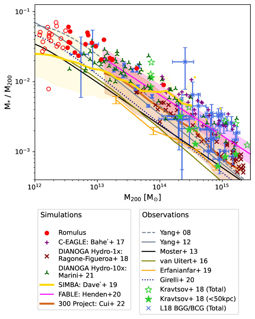
Figure 1: The Stellar Mass-Halo Mass (SMHM) relation for massive galaxies. Romulus galaxies are shown in red: BGGs (i.e. central galaxies in halos with $(M_{\rm 200}/\rm M_{\odot})\geq 10^{12.5}$) are plotted as the filled circle while open circles show central galaxies in halos with $10^{12}\leq(M_{\rm 200}/{\rm M_{\odot}})<10^{12.5}$. The stellar mass is measured within $50\,\rm kpc$ projected radius. For comparison, we overplot the results from earlier studies. Observations: Yang et al. (2008, gray dashed and sold lines); Yang et al. (2012, gray dashed and sold lines); Moster et al. (2013, black solid line); Kravtsov et al. (2018, green filled and open stars); L18 (blue $\times$ symbols with error bars); van Uitert et al. (2018, khaki solid line); Erfanianfar et al. (2019, orange solid line with error bars); Girelli et al. (2020, blue dotted line). Simulations: Bahé et al. (2017, C-EAGLE, purple $+$ symbols); Cui et al. (2022, The 300 Project, brown solid line + 95 percentile shaded band); Ragone-Figueroa et al. (2018, DIANOGA Hydro-1x, maroon $\times$ symbols);Davé et al. (2019, SIMBA, yellow solid line and shaded band); Henden et al. (2020, FABLE, magenta solid line and shaded band); Marini et al. (2021, DIANOGA Hydro-10x, dark green Y  symbols).

The Stellar Mass-Halo Mass (SMHM) relation of central galaxies reflects the halo mass dependence of a combined effect of (i) the star formation efficiency and (ii) the accretion and merger rate across cosmic time. In our halo mass range of interest, the star formation efficiency decreases with increasing halo mass (e.g., Lin & Mohr 2004; Yang et al. 2008; Yang et al. 2012; Moster et al. 2013; van Uitert et al. 2018; Kravtsov et al. 2018; Erfanianfar et al. 2019; Girelli et al. 2020). This decline is thought to be in part due to the increasing IGrM/ICM temperature with halo mass (see Mahdavi et al., 2013, and references therein) and the concommitant decrease in radiative cooling efficiency (Rees & Ostriker, 1977), and in part due to the effects of preventative SMBH feedback becoming increasingly important in massive systems (see, for instance, Binney & Tabor 1995; Ciotti & Ostriker 2001; Babul et al. 2002, 2013; McCarthy et al. 2008; Prasad et al. 2015, 2017; Cielo et al. 2018; see also recent reviews by Oppenheimer et al. 2021 Lovisari et al. 2021b as well as references therein). With suppressed star formation activity, the merger and accretion of satellite galaxies, as well as the capture of their stellar debris due to galaxy harassment and tidal disruption, play an important role in the growth of stellar mass of these galaxies (Dubinski 1998; Conroy et al. 2007; De Lucia & Blaizot 2007; Ruszkowski & Springel 2009; Laporte et al. 2013; Rennehan et al. 2020).

In Fig. 1, we plot $M_{*}/M_{200}$ as a function of $M_{200}$, where $M_{*}$ is the stellar mass of a central galaxy. For reference, we show the SMHM relation from several observational studies. The curves in different colours and line styles are from Yang et al. (2008, gray, dashed); Yang et al. (2012, gray, solid); Moster et al. (2013, black, solid); van Uitert et al. (2018, khaki, solid); Erfanianfar et al. (2019, orange, solid); Girelli et al. (2020, dotted). For Kravtsov et al. (2018), two different sets of data points based on different definition of stellar mass are presented: one based on measurements within a $50\,\rm kpc$ aperture (green filled stars) and the other based on the total mass (green open stars), calculated by integrating the stellar luminosity profile extrapolated to large distances. The difference between the two is an outcome of including the extended diffuse intragroup/intracluster light (IGrL/ICL) in stellar mass measures. The blue $\times$ symbols with error bars show BGGs & BCGs from L18 sample, selected from the Multi-epoch Nearby Cluster Survey (MENeaCS, Sand et al. 2011, Sand et al. 2012), the Canadian Cluster Comparison Project (CCCP, Bildfell et al. 2008; Mahdavi et al. 2013; Hoekstra et al. 2015; Loubser et al. 2016; Herbonnet et al. 2020), and the Complete Local Volume Groups Sample (CLoGS, O’Sullivan et al. 2017.) MENeaCS and CCCP targeted galaxy clusters while CLoGS targeted galaxy groups. For convenience, we hereby refer to the 32 galaxies from MENeaCS and CCCP as L18 BCGs, and rest of the galaxies from CLoGS as L18 BGGs. L18 BGGs are central galaxies of a subset of CLoGS comprising 14 (of 26) high-richness and 9 (of 27) low-richness groups. Only the BGGs of the high-richness groups are shown in Fig. 1 since the low-richness groups do not yet have halo mass estimates.

Estimated from various observables, the observed stellar and halo mass are dependent on details of observational techniques, definitions of the masses, as well as various assumptions informing data modeling and analysis. In Appendix A, we summarize how the observational SMHM relations presented in Fig. 1 were obtained and discuss any caveats. It is important to note that the large scatter among the observationally-based results is mostly due to the use of different methods, as well as inherent challenges in determining both the stellar and halo masses. For this reason, we compare the simulation results to a compilation of SMHM relations rather than attempt to match to one specific determination.

We also plot in Fig. 1 the SMHM relation for Romulus galaxies (red filled circles: $M_{\rm 200}/M_{\odot}\geq 10^{12.5}$, red open circles: $10^{12}\leq M_{\rm 200}/M_{\odot}<10^{12.5}$) as well as the results from a few other recent cosmological simulations: C-EAGLE (Bahé et al. 2017, purple cross), DIANOGA Hydro-1x (Ragone-Figueroa et al. 2018, maroon $\times$) and DIANOGA Hydro-10x (Bassini et al. 2020; Marini et al. 2021, dark green Y ), The 300 Project (Cui et al. 2018, 2022, brown line and shaded band), SIMBA ( Davé et al. 2019, yellow line and shaded band), and FABLE (Henden et al. 2020, magenta line and shaded band). For the latter three, the solid lines show the median while the band denotes the region encompassing 95% of the galaxies. All the stellar masses from these simulations correspond to the sum of the central galaxy and the IGrL mass within a cylinder of radius $50\,\rm kpc$ aligned along the sight line. Any contribution of resolved satellite galaxies located along the cylinder is explicitly excluded. This definition of the stellar mass is adopted for a fair comparison with the stellar mass determinations from observations.

The overall distribution of Romulus galaxies is consistent with observations especially if one takes into account the spread in the observed SMHM relation. However, the trend with increasing mass appears to be slightly shallower than the observed SMHM relation and the Romulus galaxies appear to be edging towards the upper boundary of the scatter in the observed SMHM relationships at the massive end. To be fair, this impression is largely due to just two points corresponding to the BGGs in RomulusC and G2.

On the group-scale, the DIANOGA Hydro-10x (green Y ) results are in excellent agreement with the Romulus results, including the RomulusC result. On the cluster scale, the results are comparable to the C-EAGLE (purple +) results and as Bahé et al. (2017) have pointed out, the latter are a factor of $\sim 2$ larger ($\sim 0.3$ dex) than the comparable observations of Kravtsov et al. (2018, filled green stars; $r=50\,\rm kpc$ aperture). As for SIMBA (yellow) and Fable (magenta), while their 95-percentile bands overlap with the spread in the observed SMHM relations, the SIMBA median, and to a lesser account the Fable median, do not decrease as steeply with increasing mass as the observed results. In general, most simulations tend to produce central cluster galaxies with higher than observed stellar masses, and the discrepancy grows with halo mass. This is a long-standing issue with most cosmological hydrodynamic simulations (c.f.  Ragone-Figueroa et al. 2013; Martizzi et al. 2014). Interestingly, the SMHM relations of the Gizmo-based 300 Project simulations (brown), both the band and the median curve, and DIANOGA Hydro-1x (maroon $\times$) are in very good agreement with the observations. Finally, for completeness we direct readers interested in the SMHM results for Illustris TNG100 and EAGLE to Oppenheimer et al. (2021); in brief, both give SHMHs that are similar to SIMBA and Fable but with different normalizations. To summarize, we find that current cosmological simulations, with notable exceptions of the 300 Project and DIANOGA Hydro-1x, generally have a common feature: the stellar mass of the galaxies does not decrease as steeply as the observed relations.

There are several factors that could result in higher stellar mass fraction in simulated galaxies than in the observations, particularly at the high mass end. It is well known that extended stellar envelopes grow, become more established, and hold a greater fraction of the total stellar mass in increasingly more massive halos (Zhao et al. 2015a, b, see also a recent review article by Contini 2021). The extended diffuse IGrL/ICL is not easy to detect observationally due to its low surface brightness, while in the simulations, one can count every star particle. Consequently, it is not inconceivable that observational underestimate of the BCGs’ stellar mass grows with host halo mass. Another possibility is that the feedback or the coupling of this feedback to the gas is not correctly modeled in the simulations, particularly in high mass halos, resulting in overproduction of stars in BCGs & BGGs (see Oppenheimer et al. 2021 for details). We also note that apart from feedback, it is also essential that the simulations correctly model the star formation and the disruption histories of satellite galaxies as well as the correct stellar mass accretion history onto the BCGs & BGGs (e.g., White & Rees 1978; Moore et al. 1996; Bullock & Johnston 2005; De Lucia & Blaizot 2007; Johnston et al. 2008; Groenewald et al. 2017). A comprehensive study of the co-evolution of massive galaxies and their host halo environment across the full range of group and cluster mass scales is essential for understanding their SMHM relation, among other properties.

3.2 Stellar kinematics

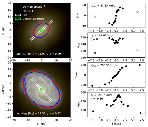
Figure 2: An illustration of the isophote fitting and the synthetic long-slit observation of the Romulus galaxies. A detailed description is given in the text. Left panels: the $20\,\rm mag\,arcsec^{-2}$ K-band isophote (blue contour) and its best-fit ellipse (red) superposed on multi-band composite images of two Romulus galaxies. The slit (white) is placed along the major axis of the ellipse (i.e., the photometric major axis) and binned to contain the equal number of stars in each bin. The central aperture (green) is used for the central velocity dispersion $\sigma_{0}$ measurement. Right panels: radial profiles of $V_{\rm LOS}$ and $\sigma_{\rm LOS}$ obtained from the synthetic long-slit observation. Measurement points beyond the $20\,\rm mag\,arcsec^{-2}$ K-band isophote are shown as open circles. These points are excluded from our analyses.

Figure 3: The scaling relationship between K-magnitude and stellar kinematics of group and cluster central galaxies. In all three panels, Romulus galaxies are presented in red. Each Romulus galaxy contributes 3 points that correspond to the measurements from 3 perpendicular line-of-sights. For comparison purposes, we also present observational results for L18 BCGs and BGGs (golden yellow and blue crosses, respectively) and $\rm ATLAS^{\rm 3D}$ galaxies (grey dots). Panel (a): the FJ scaling relation between the K-band magnitude $M_{\rm K}$ and the central velocity dispersion $\sigma_{0}$. Romulus central galaxies in halos with $\log(M_{\rm 200}/\rm M_{\odot})\geq 12.5$ are plotted as the filled circle while open circles show central galaxies in halos with $12\leq\log(M_{\rm 200}/{\rm M_{\odot}})<12.5$. The red line and shade shows a linear fit and error to Romulus results. The gray line is the joint fit to the L18 BGGs and ATLAS^3D data. Panel (b): the same as panel (a) but with Romulus galaxies differentiated based on their visual morphology (spheroids: red diamonds with black edge; disks: red crosses; and interacting: open red stars). The Romulus spheroids follow the same scaling behaviour as the L18 BGGs and ATLAS^3D galaxies, both of which are predominantly early-type systems. Panel (c): the scaling relation between $M_{\rm K}$ and the combined velocity scale $S_{\rm 0.5}$ (see the text for its definition).

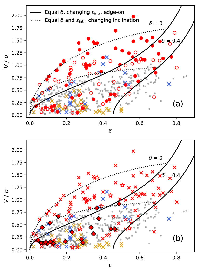
Figure 4: Panel (a): the distribution of galaxies on $v_{\rm max}/\sigma_{\rm 0}$ versus the ellipticity ($\epsilon$) plane. All the symbols are the same as Panel (a) of Fig. 3. The solid curves are the analytic solutions for axisymmetric systems viewed from edge-on with the anisotropy parameter $\delta$ of 0 (upper) and 0.4 (lower). The dotted curves show the effect of changing inclination when $\delta$ and the intrinsic ellipticity $\epsilon_{\rm intr}$ are fixed to $\delta=0$, $\epsilon_{\rm intr}=0.75$ (upper) and $\delta=0.4$, $\epsilon_{\rm intr}=0.7$ (lower). Panel (b): the same as panel (a) but with Romulus galaxies differentiated based on their visual morphology as in panel (b) of Fig. 3 (spheroids: red diamonds with black edge; disks: red crosses; and interacting: open red stars).

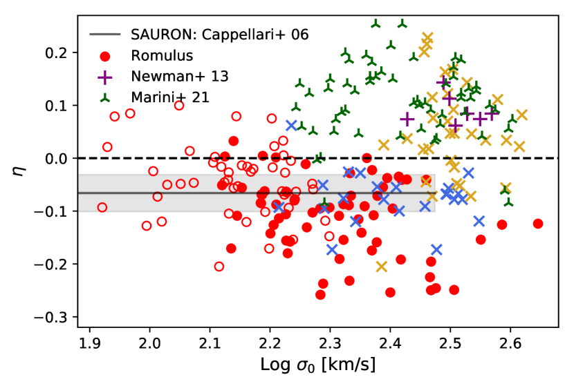
Figure 5: The dependence of the power-law index $\eta$ on $\sigma_{\rm 0}$, where $\eta$ characterizes how the velocity dispersion profile scales with radius. The purple pluses are observed BCGs from Newman et al. (2013), the blue and golden yellow crosses are the L18 BGGs and BCGs, respectively, and the gray horizontal line and shade corresponds to the mean $\eta$ and its uncertainty derived by Cappellari et al. (2006) using the SAURON galaxies. The Romulus results are shown in red: central galaxies in halos with $\log(M_{\rm 200}/\rm M_{\odot})\geq{12.5}$ are plotted as the filled circle while open circles show central galaxies in halos with ${12}\leq\log(M_{\rm 200}/{\rm M_{\odot}})<{12.5}$. The green Y  symbols show the DIANOGA Hydro-10x numerical simulation results from Marini et al. (2021).

Galaxy stellar kinematics provide valuable information about the distribution of dynamical mass, hence, the gravitational potential at the core of halos. There are observed empirical relationships, such as the Faber-Jackson relation (FJR; Faber & Jackson 1976), that hold on a wide range of scales, whereas, some relations are scale-dependent: for example, the observed velocity dispersion profiles of typical galaxies show flat or negative slopes (i.e., decreasing velocity dispersion going radially outward), while BCGs predominantly have positive slopes (Carter et al. 1999; Brough et al. 2008; Loubser et al. 2008; Newman et al. 2013; Veale et al. 2017; L18; Loubser et al. 2020). Furthermore, the ratio between the ordered rotation and the random motion dominated component ($V/\sigma$) is widely used to describe the kinematic structure of galaxies (Kormendy 1982): Conventionally, low $V/\sigma$ is associated with a dispersion-dominated spheroidal galaxy and high $V/\sigma$ to a disky galaxy with ordered rotation. However, observed galaxies display a wide range of $V/\sigma$ regardless of their visual morphology. We will return to this in Sections 3.4 and 3.3

In this section, we examine how well the Romulus simulations reproduce kinematic scaling relations and kinematic properties found in observations. For measurements of kinematic properties, we followed the specification of the spatially-resolved long-slit spectroscopic observations of L18. Unless otherwise specified, we only consider particles within a $50\,{\rm\thinspace kpc}$ radius sphere from the centers of galaxies to measure parameters presented in this section. Fig. 2 illustrates how we performed the photometric isophote fitting and the synthetic long-slit observation of the simulated galaxies. Two of the Romulus galaxies are selected as examples. The left panels are multi-band composite images generated using pynbody package (Pontzen et al. 2013) . The blue contours in the images are the $20\,\rm mag\,arcsec^{-2}$ K-band isophote. The photometric ellipticity of galaxies was measured by fitting an ellipse (red line) to this isophote in keeping with how the ellipticities of the 2MASS galaxies were determined (Jarrett et al. 2003). The dust reddening effect is not taken into account in this study.

We put a slit (the white box in Fig. 2) along the photometric major axis of the fitted ellipse (red) for a synthetic long-slit observation. In keeping with L18, we used a slit that extends $10\,\rm kpc$ on either side when analyzing galaxies from Romulus25, RomulusG1, and RomulusG2 while a larger slit extending $15\,\rm kpc$ to each side is used for the BGG of RomulusC. The vertical width of the slit is fixed to $1\,\rm kpc$ in all cases. The slit is divided into 15 spatial bins with an equal number of stars. Therefore, the bin sizes are the smallest near the center of the galaxy due to the high number density of stars there and become progressively larger towards the outskirts. Using the stars from each bin $i$, we measured the mean line-of-sight velocity ($V_{\rm LOS,i}$, the first moment) and the line-of-sight velocity dispersion ($\sigma_{\rm LOS,i}$, the second moment), weighted by the V-band luminosity of each particle (see the right panels of Fig. 2). Results from bins beyond the $20\,\rm mag\,arcsec^{-2}$ isophote (shown as open circles in the $V_{\rm LOS}$ and $\sigma_{\rm LOS}$ profiles) were not considered for further analyses (e.g., see the example at the top panel of Fig. 2; the outer most data points presented with an open circle are rejected).

Using $V_{\rm LOS,i}$ and $\sigma_{\rm LOS,i}$ measurements along the slit, we calculated the rotational velocity and the velocity dispersion profiles of the galaxies. Following L18, we use the maximum of the velocity curve, $V_{\rm max}=[max(V_{\rm LOS,i})-min(V_{\rm LOS,i})]/2$, as a summary measure of the ordered rotational component and we use the power-law index $\eta$, where $\sigma_{\rm LOS}(R)\propto R^{\eta}$, $R$ is the distance along the major axis from the galactic center, to characterize whether the velocity dispersion is rising or falling with radius. We measured the central velocity dispersion $\sigma_{0}$ of each galaxy within an aperture (the green box in Fig. 2) of a size of $1\,\rm kpc\times 1\,\rm kpc$ on each side from the center of the Romulus25, RomulusG1, and RomulusG2 galaxies and $5\,\rm kpc\times 1\,\rm kpc$ for the RomulusC BCG, in keeping with L18. Throughout the paper, we use $V_{\rm max}/\sigma_{\rm 0}$ to denote $V/\sigma$ estimated specifically following the long-slit setting.

In Fig. 3, we present the scaling relationship between K-magnitude and stellar kinematics of central galaxies in Romulus groups. The kinematic properties of Romulus galaxies are measured from 3 different line-of-sights perpendicular to each other to capture the scatter due to inclination (see, for example, Bellovary et al., 2014); therefore, each galaxy contributes 3 data points (red symbols) in the panels. We also show observations from L18 and $\rm ATLAS^{\rm 3D}$ (Cappellari et al. 2011; Emsellem et al. 2011; Cappellari et al. 2013). The BGGs & BCGs  from L18 are colour-coded differently (blue and golden yellow, respectively) for ease of comparison. We note the CLoGS selection criteria (O’Sullivan et al. 2017) preferentially excludes groups with late type BGGs, resulting in a biased sample; among the 23 L18 subset of CLoGS BGGs, 13 are ellipticals and 7 are lenticulars. This bias needs to be factored in when comparing to simulations. Similarly, $\rm ATLAS^{\rm 3D}$ also targets early-type galaxies and these galaxies are not necessarily centrals. Additionally, $\rm ATLAS^{\rm 3D}$ includes galaxies with stellar mass higher than $6\times 10^{9}\,\rm M_{\rm\odot}$; hence, a large fraction are smaller than typical BGGs. We also note that the kinematic properties of the $\rm ATLAS^{\rm 3D}$ galaxies are measured using integral-field spectroscopy and come from a central aperture whose radius is a galaxy’s effective radius ($R_{\rm e}$) or smaller. As we discuss below, the size of the aperture relative to $R_{\rm e}$ affects the kinematic measurements.

Panel (a) of Fig. 3 shows the FJR in the K-band magnitude ($M_{\rm K}$). The gray line shows the joint fit to the L18 BGGs and $\rm ATLAS^{\rm 3D}$ galaxies (slope: $-7.05$). Overall, L18 BGGs are distributed on the extension of the scaling relation of $\rm ATLAS^{\rm 3D}$ galaxies. We attribute this consistency between the two samples in part to the fact that they are both dominated by early type galaxies. Interestingly, there appears to be a transition at $M_{\rm K}\approx-26$; the less luminous L18 BCGs are consistent with the combined L18 BGGs and $\rm ATLAS^{\rm 3D}$ FJR but the more luminous L18 BCGs manifest a slightly steeper scaling relationship like that defined by the red line. This red line (and shaded band) is the linear fit (and error) to the Romulus galaxies (slope: $-8.69\pm 0.77$).

In panel (b) of Fig. 3, we demonstrate that the difference between the red and black lines is mainly due to difference in the galaxies comprising the two samples: the Romulus sample includes both early and late type galaxies and while the $\rm ATLAS^{\rm 3D}$ galaxies and L18 BGGs are primarily early type systems. The data points shown in this plot are the same in panel (a) except that we classify the Romulus based on their visual morphology. We discuss in detail how the galaxies were classified in Section 3.3. The red diamonds with black edge correspond to the spheroids; the red crosses to disk galaxies; and open red stars to interacting galaxies. All other symbols are the same as in panel (a). As the plot shows, the distribution of the Romulus spheroids is consistent with that of L18 BGGs and $\rm ATLAS^{\rm 3D}$ galaxies. The Romulus disk and interacting galaxies, however, track a different scaling relationship. There are BGG catalogues, such as those discussed by Weinmann et al. (2006) and Gozaliasl et al. (2016), that contain a sizeable fraction of late type, star forming BGGs. These are not shown in Fig. 3 because their kinematic properties are not available but we will discuss these samples further in subsequent sections.

To eliminate the morphological dependence of the kinematic scaling relations, Weiner et al. (2006) introduced a ‘combined velocity scale’, defined as, $S_{\rm K}\equiv\sqrt{\rm KV^{2}+\sigma^{2}}$, where K is a normalization constant equal to or smaller than 1. This parameter combines the rotational and the random characteristics of a galaxy. Kassin et al. (2007) showed that $S_{\rm 0.5}$ tightly correlates with the galaxy mass, regardless of the morphology. As shown in panel (c) of Fig. 3, Romulus galaxies successfully reproduce a linear scaling relation between $M_{\rm K}$ and $S_{\rm 0.5}$ with reduced scatter. The distribution of L18 BGGs (blue) as well as $\rm ATLAS^{\rm 3D}$ galaxies (gray) are also in much better agreement with that of Romulus galaxies, as are the L18 BCGs (golden yellow). This further supports the assertion that the differences between these samples in Panel (a) is mainly due to the morphological diversity in Romulus sample, or lack thereof in L18 galaxies.

Panel (a) of Fig. 4 shows the distribution of galaxies on the $V/\sigma$ versus the projected ellipticity ($\epsilon$) plane. A galaxy’s inclination as well as its anisotropy parameter, $\delta=1-\Pi_{\rm zz}/\Pi_{\rm xx}$ where $\Pi_{\rm ij}=\int\rm d^{3}x\rho\sigma_{\rm jk}^{2}$ (Binney 1978; Binney 2005), can affect where it sits on this plane as illustrated by the black solid and dotted lines. The black lines present how the projected ellipticity and $V/\sigma$ of an axially symmetric oblate rotating system, viewed edge-on, changes as the galaxy’s intrinsic ellipticity ($\epsilon_{\rm intr}$) is varied. The two curves correspond to $\delta=0$ and $\delta=0.4$. The dotted lines show the result of changing inclination. The upper and lower curves correspond to systems with ($\delta=0$, $\epsilon_{\rm intr}=0.75$) and ($\delta=0.4$, $\epsilon_{\rm intr}=0.7$), respectively.

As for the observations, the $\rm ATLAS^{\rm 3D}$ galaxies (grey points) span a range of $V/\sigma$ and $\epsilon$. This is not surprising since the sample includes both fast and slow rotating early type galaxies, with fast rotators preferentially being the lower mass systems (Emsellem et al. 2011). Overall, however, the points fall below the lower dotted curve and are somewhat more concentrated in the lower left quadrant (rounder projected images). The L18 BGGs (blue crosses) have a similar distribution to the $\rm ATLAS^{\rm 3D}$ points, with many of the central galaxies exhibiting non-trivial bulk rotation. This is in keeping with recent MUSE results presented in (Olivares et al., 2021). The L18 BCGs, however, have typically lower $V/\sigma$. The Romulus galaxies are, as usual, denoted by red points. Collectively, the red points span a wider range of $\epsilon$ and $V/\sigma$ than the L18 BGGs and the $\rm ATLAS^{\rm 3D}$ points. As shown in panel (b) of Fig. 4, this too is due to the morphological diversity of the Romulus galaxies, and lack thereof in the $\rm ATLAS^{\rm 3D}$ galaxies and the L18 BGGs. The distribution of Romulus galaxies with spheroidal morphology (red diamonds with black edges) matches that of L18 and $\rm ATLAS^{\rm 3D}$ samples. Most of the Romulus galaxies above lower dotted curve are disk galaxies (red crosses).

In Fig. 5, we consider how the velocity dispersion profile scales with radius. Specifically, we plot the power-law index ($\eta$) versus the central velocity dispersion ($\sigma_{\rm 0}$). The vast majority of the galaxies with $\sigma_{0}{\;\raise 1.29167pt\hbox{$<$\kern-7.5pt\raise-4.73611pt\hbox{$\sim$}}\;}2.45$ are BGGs and these have negative $\eta$ values. This includes most of the Romulus galaxies (red filled and open circles), the L18 BGGs (blue crosses) and the early type galaxies that comprise the SAURON sample (Cappellari et al. 2006; gray line and shaded area). In contrast, nearly all of simulated BGGs with $\sigma_{0}{\;\raise 1.29167pt\hbox{$<$\kern-7.5pt\raise-4.73611pt\hbox{$\sim$}}\;}2.45$) from the DIANOGA Hydro-10x simulations Marini et al. (2021) have positive $\eta$ values. For $\sigma_{0}{\;\raise 1.29167pt\hbox{$>$\kern-7.5pt\raise-4.73611pt\hbox{$\sim$}}\;}2.45$, the spread of $\eta$ for the observed galaxies (e.g. L18 and Newman et al. 2013 BCGs) broadens and spans both positive and negative $\eta$ values. In fact, majority of the galaxies tend to have positive $\eta$s. This change in behaviour is well known. A number of studies have noted that on the group-scale and lower, the stellar velocity dispersion profile of the central galaxies tend to decrease with increasing radius. On the cluster-scale, the BCGs typically have rising velocity dispersion profiles with increasing radius (Von Der Linden et al. 2007; Bender et al. 2015; Veale et al. 2017). The origin of this flip is still not well understood. We leave a more detailed investigation of this change to future work. Here, we simply mention two possible explanations: The change in slope may be a reflection of the differences in the dynamical state (e.g., mass-to-light ratio; M/L) at the outskirts of BCGs (Dressler 1979; Fisher et al. 1995; Sembach & Tonry 1996; Carter et al. 1999; Kelson et al. 2002; Loubser et al. 2008; Newman et al. 2013; Schaller et al. 2015; Marini et al. 2021), or it could be due to increased contribution from the intragroup/intracluster light along the line-of-sight and the increased leverage of tangential orbits (Loubser et al. 2020). All of these effects are linked to the increased frequency of galaxy-galaxy interactions and more specifically, central-satellite interactions, implicated in the build-up of extended diffuse stellar component. And, as discussed by Schaye et al. (2015); Oppenheimer et al. (2021), the EAGLE simulations clearly show that the extended stellar halo becomes increasingly more important, and hosts a non-trivial fraction of the total stellar mass towards the cluster scale.

3.3 Visual morphology

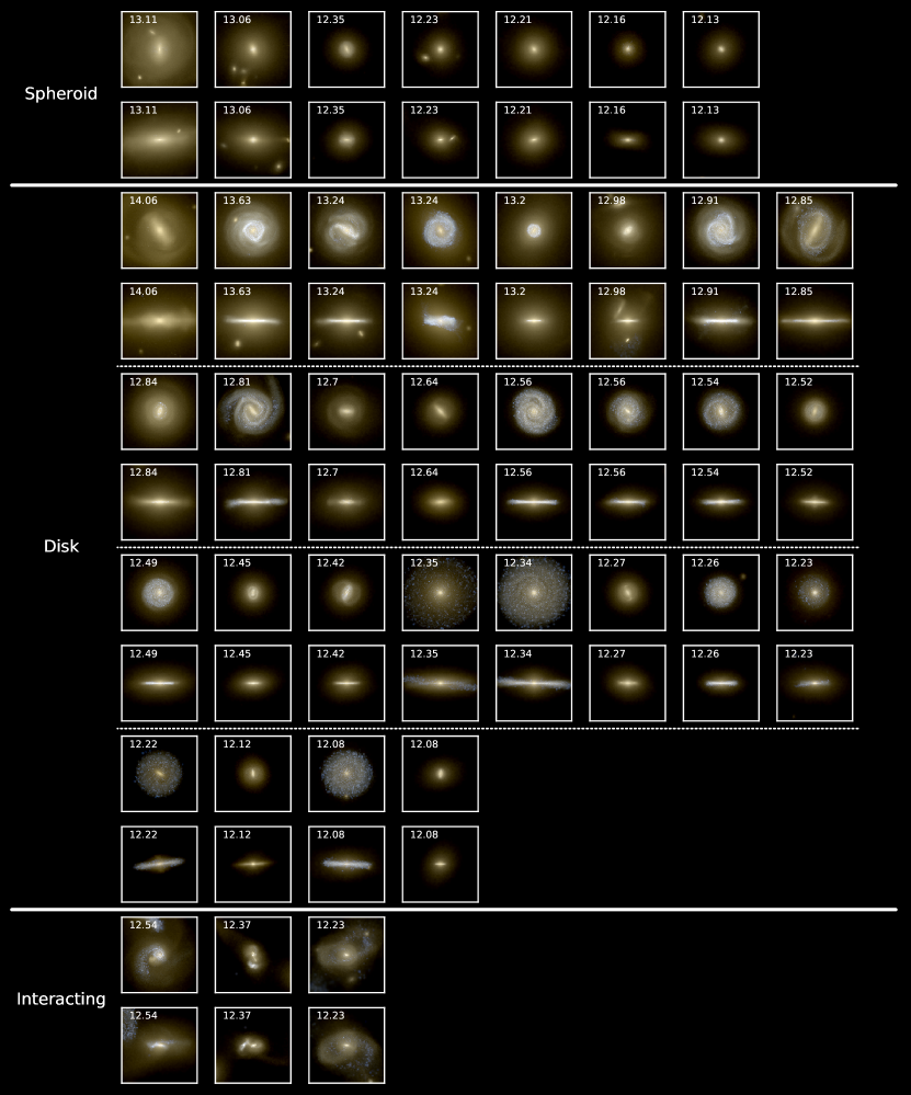
Figure 6: Multi-band composite image of Romulus galaxies viewed from face-on and edge-on. The size of each box is $50\,\rm kpc$ and the images were scaled to reach maximum surface brightness of $26\rm\,mag\,arcsec^{-2}$. The galaxies are grouped according to their visual morphology and sorted by their halo mass ($\log M_{\rm 200}$) shown in the top left corner of each panel.

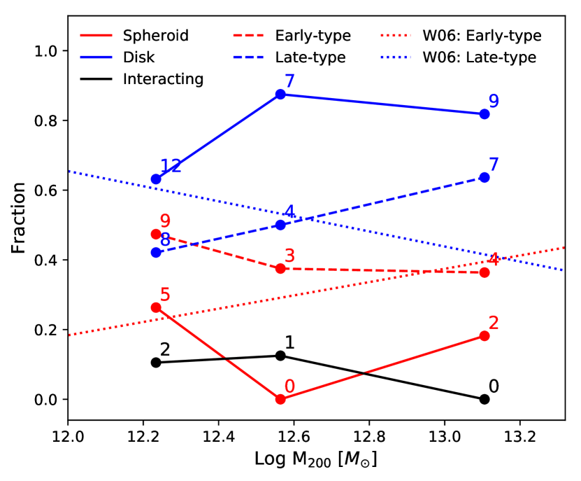
Figure 7: The fraction of each morphology type as a function of the halo mass. Solid lines show the fractions from the visual morphology classification (red: spheroid, blue: disk, black: interacting) and dashed lines are from the colour–Sérsic index classification scheme (red: early-type, blue: late-type). Numbers near the data points are the number of galaxies in each bin. The lowest halo mass bin corresponds to $12\leq\log(M_{*}/{\rm M_{\odot}})\leq 12.5$. Galaxies in this halo mass range are not BGGs as per our definition and the results for these galaxies are shown as open red circles in the other plots. The middle mass bin corresponds to the 8 lowest mass Romulus groups while the rightmost bin comprises the remaining set of more massive groups. The observed early-type and the late-type fractions from W06 are shown as dotted lines for comparison.

It is commonly suggested that the visual morphology of a galaxy reflects its formation and interaction history (e.g., Conselice 2006; Driver et al. 2006; Benson et al. 2007; Ilbert et al. 2010). A disky morphology is associated with relatively quiescent recent merger history, recent star formation activity and possibly even, fresh influx of fresh gas. A spheroidal morphology, on the other hand, is associated with strong galaxy-galaxy interactions and moderate-major mergers, particularly dry mergers.

Traditionally, the visual morphology of observed galaxies is determined via a visual inspection. Given its high resolution, Romulus suite allows us to perform visual morphology classification of galaxies in a manner similar to that of observers. Fig. 6 shows the mock multi-band images of entire Romulus BGG sample viewed both edge-on and face-on. These mock images confirm that the Romulus BGGs span the full spectrum of morphological types found in observations. We have visually classified the galaxies into 3 morphological types: spheroids, disks, and disturbed (with on-going interactions). We set aside the disturbed or irregular galaxies and focus exclusively on the spheroids and the disks here.

There are also quantitative morphology indicators that have been used to classify photometric observations, such as the Sérsic index, concentration, asymmetry parameter, or disk-to-total ratio derived from photometric bulge-disk decomposition. In the latter case, the observed light profiles are characterized by the fraction of the spheroidal component with respect to the total stellar mass, i.e., the spheroidal-to-total ratio (S/T). The 2D projected light profiles of galaxies are fitted with a bulge-component that follows the Sérsic profile (Sersic 1968) and a disk-component with the exponential profile (Freeman 1970).

We have carried out a quantitative classification of the Romulus BGGs based on their $u-r$ colour and Sérsic index. This classification scheme was used in Deeley et al. (2017), where they separated their galaxies into red, high Sérsic index early-type galaxies and blue, low Sérsic index late-type galaxies. Comparing these results to those from visual classification, we find that all of our Romulus BGGs that were visually identified as spheroids are also identified as early-type galaxies when classified using the colour-Sérsic index criterion. On the other hand, only 19 of 28 visual disk galaxies are classified as the late-types. The remaining 9 galaxies possess a disky structure but were not classified as late-types because their disks consists of a relatively old stellar population (i.e., red in colour) and/or the overall light profile is dominated by high Sérsic index components.

Fig. 7 shows the fraction of each morphological type as a function of the halo mass. Both the results from visual (solid line) and quantitative (dashed line) morphology classification results are presented. For comparison, we also plot the early- and the late-type fractions of observed group central galaxies (W06; red and blue dotted lines, respectively) in the SDSS-based New York University Value-Added Galaxy Catalogue (Blanton et al., 2005). The galaxies are classified according to a quantitative criteria utilizing both the galaxies’ $(g-r)$ colour and their specific star formation rate (i.e., red, quiescent early-type and blue, star forming late-type galaxies). The W06 sample is both large and spans a wide range of halo mass. W06 find that ${\sim}50\%$ (${\sim}30\%$) of the centrals in low-mass groups are late-types (early-types), while the fraction is around $40\%$ ($40\%$) in massive groups. This trend, of decreasing late-type fraction with halo mass, is comparable to that noted by Gozaliasl et al. (2016) in their low-redshift samples.

Comparing our quantitative classification results to those of W06’s quantitative classification, we find that the morphological mix of the BGGs from the 8 lowest mass Romulus groups (the middle points) is in good agreement with W06’s findings. However, the fraction of late-type BGGs in Romulus increases when we consider the remaining set of more massive groups. This is an indication that Romulus simulations are straining in the regime of massive groups and at least some of the properties of the corresponding BGGs are deviating from observations.

3.4 Spheroid to total ratio (S/T)

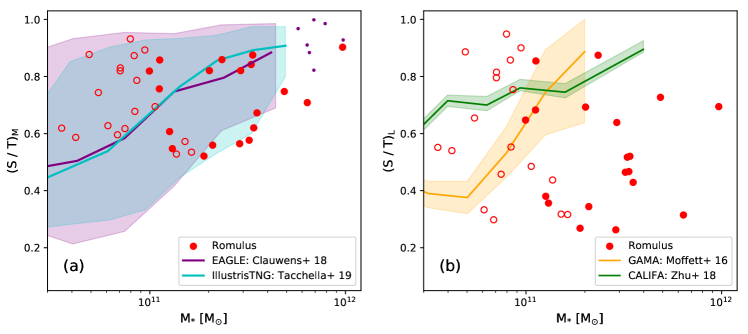
Figure 8: The stellar mass dependence of S/T. Romulus galaxies are shown in red in both panels. Panel (a) compares the mass-weighted S/T from numerical simulation studies: EAGLE (Clauwens et al. 2018; purple line and dots, the shaded area encloses the 10-90 percentiles), and Illustris TNG100 (Tacchella et al. 2019; cyan line, the shaded area shows the $1\sigma$ scatter). In panel (b), we present the luminosity-weighted S/T of Romulus galaxies and observationally derived S/T for galaxies in GAMA (Moffett et al. 2016; orange) and CALIFA (Zhu et al. 2018; green) surveys. The former is based on photometric decomposition while the latter is utilizes stellar kinematics. Specifically, the CALIFA result is a luminosity-weighted, kinematically informed S/T.

A number of simulation studies have demonstrated that the photometric S/T may be biased in terms of the information they provide about the overall structural properties of galaxies; in other words, there is often discrepancy between the kinematically identified morphology and visually or photometically defined morphology. Photometric measurements systematically underestimate the spheroidal component compared to the kinematic measurements (e.g., Scannapieco et al. 2010; Bottrell et al. 2017).

The simplest kinematic analyses start by decomposing the stars’ orbital motions into ordered and random motion, and the ratio between the random and the ordered components is often adopted as a parameterization of the structure of galaxies. It is suggested by numerical studies that the kinematic structure of galaxies is closely related with the growth and interaction history of galaxies (Abadi et al. 2003; Scannapieco et al. 2009; Scannapieco et al. 2010; Stinson et al. 2010; Sales et al. 2010; Zavala et al. 2016; Correa et al. 2017; Clauwens et al. 2018; Tacchella et al. 2019; Park et al. 2019).

Recently, with Integral Field Spectroscopy observations available, the kinematic structure of a galaxy based on the stellar dynamics is determined by building a 3D model using either (i) Jeans anisotropic modelling (i.e., JAM, Jeans 1922, as implemented in Cappellari 2008), or when data quality allows, (ii) Schwarzschild modelling (Schwarzschild 1979) where a set of orbits is constructed that the superposed stellar distribution matched the observed 2D surface brightness and stellar kinematics (van den Bosch et al. 2008; van de Ven et al. 2008; Zhu et al. 2018; van de Sande et al. 2020). This technique allows the kinematic S/T measurement of observed galaxies.

In numerical simulations, it is straightforward to measure 3D kinematic properties of stars since the full 6D phase space information of the particles is available. Generally, the definition of the kinematic S/T is based on the orbital circularity of stellar particles defined as $\epsilon_{\rm J}=J_{\rm z}/J_{\rm circ}(E)$, where z is the net spin axis of a galaxy, $J_{\rm z}$ is a z-component of the specific angular momentum of a particle, and $J_{\rm circ}(E)$ is a specific angular momentum expected if a particle was in a circular orbit with the same orbital energy (Abadi et al. 2003). By definition, stars with their angular momentum vectors well aligned with the bulk spin of a galaxy have $\epsilon_{\rm J}\sim 1$ and stars with the random orbits show the distribution of $\epsilon_{\rm J}$ that peaks at 0.

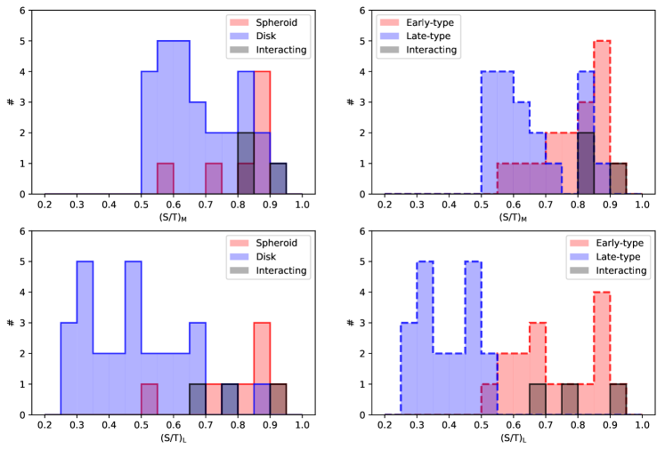
Figure 9: The comparison of the distributions of (S/T)_M (top row) and (S/T)_L (bottom row) versus BGGs’ visual morphology (right column) and morphology based on color and Sérsic index (right column). (S/T)_L is much more strongly correlated with the visual and especially the quantitative classification schemes. All early-type galaxies have (S/T)${}_{\rm L}>0.53$ and all late-type galaxies have (S/T)${}_{\rm L}<0.53$.

In this study, we present two different definitions of S/T for Romulus galaxies: mass-weighted (S/T)_M and V-band luminosity weighted (S/T)_L. The reason for doing so is to facilitate a fair comparison of our results to both prior numerical and observational studies. The stellar mass and the (S/T) presented here are measured within a sphere of radius $R=50\,\rm kpc$ but we have confirmed that the value of (S/T) is not sensitive to the change in the aperture size, e.g., to $25\,\rm kpc$. Fig. 8 shows the stellar mass dependence of mass-weighted (S/T)_M (left panel) and the luminosity-weighted (S/T)_L (right panel). Romulus galaxies are shown in red in both panels.

For (S/T)_M, we followed the same definition as Tacchella et al. (2019): The mass of spheroidal component is defined as the sum of the mass of stellar particles with $\epsilon_{\rm J}<0.7$ and the 15% of $\epsilon_{\rm J}>0.7$ particles ($S=M_{*,\epsilon_{\rm J}<0.7}+0.15M_{*,\epsilon_{\rm J}>0.7}=0.85M_{*,\epsilon_{\rm J}<0.7}+0.15$). Including a fraction of mass of $\epsilon_{\rm J}>0.7$ particles is to take account of stars that have random orbits but their direction of angular momentum close to the bulk rotation by coincidence. Tacchella et al. (2019) applied this analysis to central galaxies with stellar masses $9\leq\log(M_{*}/{\rm M_{\odot}})\leq 11.5$ extracted from the Illustris TNG100 simulation (in Fig. 8, the cyan line is their median result and the shaded region is the $1\sigma$ scatter). Similarly, Clauwens et al. (2018) analyzed central galaxies with $\log(M_{*}/{\rm M_{\odot}})>9$ from the EAGLE. Their median result is shown in Fig. 8 panel (a) as the purple curve and the shaded region spans the 10th-90th percentiles. We note that Clauwens et al. (2018) adopted a slightly different definition of the spheroidal component ($S=2M_{*,\epsilon_{\rm J}<0}$); however, we have confirmed, as did Tacchella et al. (2019), that the precise definition of (S/T)_M does not affect the overall results discussed in this section.

All of the Romulus BGGs have stellar mass dominated by stars with random orbits, i.e., (S/T)${}_{\rm M}>0.5$ although $\sim 5$ (out of 39) sit close to this threshold. Comparing the simulations to each other, we find that they are all broadly consistent with each other. We do note, however, that the large spread in the (S/T)_M across all simulations makes it difficult to discern any statistically significant differences among them.

In panel (b) of Fig. 8, we compare the results to two observational results that derive S/T in different ways. Moffett et al. (2016, orange line line with shaded region) performed a photometric decomposition of 7506 galaxies from GAMA (Galaxy and Mass Assembly) survey and derived the fraction of the stellar mass budget in spheroidal component (i.e., elliptical galaxies and bulges of disk galaxies) and disk component. In contrast, Zhu et al. (2018, green line with shaded region) constructed 3D orbital models of 250 galaxies from the CALIFA survey and estimated the fraction of cold ($\epsilon_{\rm J}>0.8$), warm ($0.25<\epsilon_{\rm J}<0.8$), hot ($-0.25<\epsilon_{\rm J}<0.25$), and counter-rotating ($\epsilon_{\rm J}<-0.25$) orbits. Neither survey are restricted to group central galaxies. To facilitate comparison with the CALIFA results especially, we adopt the same prescription as Tacchella et al. (2019): $S/T=1-1.5f_{\rm cold}$, where $f_{\rm cold}$ is the fraction of the cold orbits. Both the observational results find that (S/T)_L increases as the stellar mass increases, though at different rates.

The luminosity-weighted (S/T)_L of Romulus BGGs shares the same definition of the spheroidal component with its mass-weighted counterpart (S/T)_M, i.e., the definition based on the orbital circularity $\epsilon_{\rm J}$, but now, this ratio is luminosity weighted and therefore, is the ratio of the luminosity of the spheroidal component to the total luminosity of the system.

Comparing the distribution of (S/T)_M and (S/T)_L of Romulus BGGs, as shown in panels (a) and (b) respectively, we notice that (S/T)_L of many of the galaxies is smaller than (S/T)_M. This is due to the fact that stars comprising disks are in general younger, and therefore, brighter than spheroid stars (see, e.g., Fig. 6). Therefore, (S/T)_L of galaxies with disks is underestimated compared to (S/T)_M. (S/T)_L, however, is a more appropriate measure for comparison with observations.

We illustrate this in Fig. 9. In the top row, we show the histogram for (S/T)_M. In the left panel, the histogram is shaded according to the Romulus BGGs’ visual morphological classification and in the right panel, by their quantitative classification. (S/T)_M does not appear to have the power to discriminate between the morphologies. In the bottom row, we show the same but for (S/T)_L. (S/T)_L is much better aligned with the BGGs’ morphology. Looking at the bottom right panel, we see that all early-type galaxies have (S/T)${}_{\rm L}>0.53$ and all late-type galaxies have (S/T)${}_{\rm L}<0.53$; therefore, the use of (S/T)${}_{\rm L}=0.53$ as a discriminator, the fractions of early- and late-type galaxies as a function of $M_{\rm 200}$ are identical to those derived using the quantitative classification.

Finally, we note that one prominent feature in panel (b) of Fig. 8 is the presence of Romulus BGGs with low (S/T)_L at the high stellar masses. This is essentially the manifestation of the same issue noted previously: Romulus produces a higher fraction of disk galaxies compared to observations (Section 3.3).

3.5 Star formation rate

Figure 10: The star formation rate and stellar mass relation at $z=0$. Romulus galaxies are coloured red. The stellar mass is measured within $50\,\rm kpc$ projected radius. The lines show the star-forming main sequence from various sources: (black solid line – observed galaxies in Whitaker et al. 2012; black dashed line – extrapolation of the Whitaker main sequence; purple, cyan, yellow curves – main sequence from EAGLE, Illustris TNG100, and SIMBA from Davé et al. 2020). The gray $\times$ symbols, green $+$ symbols, blue and golden yellow $\times$ symbols, and magenta $\square$ symbols show results for observed BGGs & BCGs  from Mittal et al. (2015), Gozaliasl et al. (2016) low-redshift samples (SI and SII), Loubser et al. (2018), and Cooke et al. (2018), respectively. The black dot-dashed line tracks the Whitaker (and extension) main sequence but is shifted down by 0.75 dex. Galaxies below this line are considered quenched. The table shows the number of quenched BGGs ($\log M_{\rm 200}\geq 12.5$) as fraction of the total number in each stellar mass bin.

The evidence of the star formation regulated by mass-dependent processes manifests as a power-law scaling relation between the stellar mass and the star formation rate ($SFR\propto M_{*}^{\alpha}$) of star-forming galaxies, i.e., the star-forming main sequence (Brinchmann et al. 2004; Noeske et al. 2007; Elbaz et al. 2011; Whitaker et al. 2012; Speagle et al. 2014). “Normal” star-forming galaxies are on the main sequence within a small scatter of about 0.2-0.4 dex (Ilbert et al. 2015; Popesso et al. 2019). As galaxies undergo star formation quenching processes, they leave the main sequence and move to the lower SFR region (e.g., Salim et al. 2007; Peng et al. 2010; Schawinski et al. 2014; Tacchella et al. 2016).

Fig. 10 shows the distribution of Romulus galaxies on the SFR-stellar mass plane at $z=0$. For reference, we also plot the observed main sequence from Whitaker et al. (2012) and its extrapolation to higher masses (black solid and dashed lines). Additionally, we also show the main sequence curves from several cosmological simulations (purple: EAGLE, cyan: Illustris TNG100, yellow: SIMBA; all from Davé et al. 2020) as well as observational results for BGGs & BCGs from different samples: (i) Mittal et al. (2015, gray $\times$ symbols) data points are based on a sample of BCGs in cool core clusters, (ii) Gozaliasl et al. (2016, green $+$ symbols) galaxies are BGGs & BCGs in their samples SI and SII hosted by X-ray bright galaxy groups and clusters in XMM–LSS, COSMOS, and AEGIS surveys, (iii) from the L18 sample, we show the results for a handful of CCCP and MENeaCS BCGs (golden yellow $\times$ symbols), as well as results for the L18 subset of CLoGS BGGs (blue $\times$ symbols). (iv) Cooke et al. (2018, magenta $\square$ symbols) sample contains BCGs from the COSMOS survey. It should be noted that SFRs derived from observations depend on the selection criteria of the individual samples as well as details of measurement methods, such as SFR indicators used and statistics used to fit these (see, e.g., Popesso et al. 2019). Details on how the star formation rates were derived from each set of observation are presented in Appendix A.3.

Galaxies can be classified as star-forming or quenched depending on their location on the SFR-stellar mass plane. In this paper, we refer to galaxies with star formation rates that are more than $0.75\,\rm dex$ below the Whitaker et al. (2012) main sequence (and its extension) as “quenched”. This demarcation line appears in Fig. 10 as a dot-dashed line. Note that this definition does not differentiate between BGGs with low and unresolved SFRs and those with low-but-measurable SFRs. In the simulations, the distinction between these two classes of quenched galaxies depends on the resolution. As discussed by Oppenheimer et al. (2021, see also references therein), there is also no observational basis for doing so since measuring low SFRs using available observational diagnostics is difficult and subject to large uncertainties.

The distribution of BGGs & BCGs in Fig. 10 show that not all observed BGGs & BCGs  are quenched: $30\%$ of the SI and SII Gozaliasl et al. (2016, green $+$ symbols) BGGs between $10^{\rm 9.5}<M_{*}/\rm M_{\odot}<10^{\rm 12}$, all of the Mittal et al. (2015, gray $\times$ symbols) BCGs, as well as a subset of L18 BCGs that are blue-core galaxies are star-forming systems (only a few of the latter, those with available SFRs, are shown in Fig. 10). Overall, $\sim 25-30\%$ of the BCGs in massive clusters are star-forming (c.f.  Bildfell et al., 2008) and based on the Gozaliasl et al. (2016) samples SI and SII results, a similar fraction of the BGGs (i.e. ${\sim}30\%$) are also star forming.

Romulus produces both quenched and star-forming central galaxies, with the overall star forming fraction being $63\%$ for the BGG population and $60\%$ if one considers all central galaxies with stellar mass $\log(\rm M_{*}/\rm M_{\odot})>10.5$. These fractions are about twice the observed results. Also, although the number of Romulus galaxies is relatively small, if we consider all the central galaxies with stellar mass $\log(\rm M_{*}/\rm M_{\odot})>10.5$, there is a trend with stellar mass: the fraction of quenched central galaxies decreases with increasing stellar mass (57% to 33% to 14%). The observed quenched fraction, however, appears to remain approximately constant.

As for the other simulations (see also, recent review by Oppenheimer et al. 2021), we find that the overall fraction of quenched BGGs & BCGs in SIMBA and Illustris TNG100 is $88\%$, and $83\%$, respectively. Both of these are higher than the observed fraction (${\sim}70\%$). In SIMBA, the quenched fraction is mostly independent of stellar mass while in Illustris TNG100, the fraction decreases with increasing stellar mass, like in Romulus, matching the observed fraction for $\log(\rm M_{*}/\rm M_{\odot})>11.5$. In EAGLE, the fraction of quenched BGGs & BCGs  in the $[10^{10.5}-10^{11}]\;\rm M_{\odot}$ stellar mass bin (${\sim}57.7\%$) is comparable to that in Romulus (${\sim}53\%$) and lower than the observed fraction. The EAGLE quenched fraction increases with stellar mass, but remains on the low side.

4 What determines the star-formation status of BGGs?

The results in the preceding section show that while the Romulus BGGs in low mass groups are in very good agreement with a number of different available observations, collectively the properties of BGGs in high mass groups are starting to diverge. Specifically, ${\sim}60\%$ of the BGGs are classified as late-type, star forming galaxies. In this section, we take a first stab at identifying the physical processes in the simulations that are responsible for the Romulus BGGs’ star formation status since this is closely linked to their kinematic and morphological properties.

4.1 The cold gas mass

Figure 11: The comparison of the cold ($T<2\times 10^{4}\,\rm K$) gas mass between the star-forming (filled symbols) and the quenched (open symbols) Romulus galaxies. The shape of the symbols correspond to the halo mass range (circle: $12.0\leq\log(M_{\rm 200}/\rm M_{\odot})<12.5$; triangle: $12.5\leq\log(M_{\rm 200}/\rm M_{\odot})<12.8$, and square $12.8\leq\log(M_{\rm 200}/\rm M_{\odot})$). The colour denotes the distance from the star-forming main sequence ($\Delta MS$) as defined in the text. The dashed line at $\log(M_{\rm gas,cold}/\rm M_{\odot})\approx 9.25$ shows a rough separation between the star-forming/quenched populations.

The first step is to determine how much cold gas there is in the galaxies. In general, there is a well-established connection between the amount of cold gas in a galaxy and its star formation status (Kennicutt-Schmidt law; Kennicutt 1998). Here, we examine the cold gas mass in star-forming and quenched Romulus BGGs at $z=0$. We define “cold gas” as any gas (particles) with temperature $<2\times 10^{4}\,\rm K$ and within $50\,\rm kpc$ of the halo center. In Fig. 11, the colour of the points corresponds to the distance, in log-scale, from the star-formation main sequence at a fixed stellar mass:

$$\Delta MS=\log(\rm{SFR})-\log(\rm{SFR}_{\rm MS}),$$ (1)

where SFR_MS is the star formation rate of the main sequence at the stellar mass under consideration. As defined in Section 3.5, galaxies with $\Delta MS<-0.75$ are considered as the quenched population and shown as open symbols, while star forming systems are denoted by filled symbols. The circles are massive galaxies in halos with $12.0\leq\log(M_{\rm 200}/M_{\odot})<12.5$; the triangles correspond to BGGs in intermediate mass groups, i.e., $12.5\leq\log(M_{\rm 200}/M_{\odot})<12.8$ and squares to BGGs in high mass groups. The amount of cold gas in Romulus BGGs is not unusual. As shown by O’Sullivan et al. (2018), many of the CLoGS BGGs have comparable or greater amount of cold gas, defined as M(HI)+M(H₂). The Romulus results suggest a threshold in the mass of cold gas between the quenched and star-forming galaxies at $\log(M_{\rm gas,cold}/M_{\odot})\approx 9.25$. Galaxies with cold gas exceeding this threshold are star forming.

4.2 The entropy profile

Table 2: Properties of galaxies presented in Section 4.3 at $z=0.06$.

Halo ID	$\log M_{\rm 200}/\rm M_{\odot}$	$\log M_{*}/\rm M_{\odot}$	SFR [$\rm M_{\odot}yr^{-1}$]	SF status	Visual morphology
99966	12.79	11.32	24.74	SFing	Disk
18714	12.84	11.51	7.57	SFing	Disk
42778	12.85	11.53	0.57	Quenched	Disk
82151	13.12	11.70	2.17	Quenched	Spheroid
65502	13.24	11.49	2.44	Quenched	Spheroid + SFing ring
G2	13.58	11.76	105.77	SFing	Disk

Figure 12: The left panel shows the IGrM entropy profile of Romulus (red and cyan) and CLoGS (black dashed; O’Sullivan et al. 2017) groups. Romulus sample is divided into two: those with star-forming BGGs and those with quenched BGGs based on the criterion adopted in Section 3.5 ($0.75\,\rm dex$ from the star-forming main sequence). The y-axis is scaled by the entropy at $5\,\rm kpc$ to facilitate the comparison of the slopes of the CLoGS and the Romulus entropy profiles. We show $K\propto R^{0.7}$ (gray dot-dashed line, Panagoulia et al. 2014) and $K\propto R^{1.1}$ (gray dotted line, Lewis et al. 2000; Babul et al. 2002; Voit et al. 2005) for reference. The right panel shows the IGrM temperature profiles of the Romulus groups. The radial coordinate of the profiles are scaled by $R_{\rm 500}$ of the individual halos while the temperatures are scaled by each halo’s IGrM temperature at $R_{\rm 500}$. The red profiles correspond to groups hosting quenched BGGs while the cyan profiles correspond to groups hosting star-forming BGGs.

Having established the presence of cold gas in the Romulus BGGs and specifically, the relationship between this cold gas and the galaxies’ star formation status, the next question is: where did it come from? On the cluster scale, whether or not a BCG is star forming depends on the radiative cooling efficiency of its X-ray emitting ICM. A common proxy of the latter is the shape of the ICM’s radial entropy profile (c.f.  Balogh et al., 1999). Non-cool core clusters are characterized by broad, nearly flat entropy cores in the central regions of the clusters. At the other end of the spectrum, the cool core clusters with star forming “blue core” BCGs are characterized by declining entropy profiles towards the cluster center (e.g., Bildfell et al. 2008; Rafferty et al. 2008; Hoffer et al. 2012; Liu et al. 2012; Rawle et al. 2012).

The entropy profiles inferred from X-ray observations of galaxy groups differ significantly from those of galaxy clusters. Specifically, non-cool core groups do not have flat entropy cores like their cluster-scale counterparts while the entropy profiles of cool core groups are not as steep as the profiles of the cool core clusters, which mostly follow the self-similar profile ($K\propto R^{\rm 1.1}$, gray dotted line, Lewis et al. 2000; Babul et al. 2002; Voit et al. 2005). In the left panel of Fig. 12, we plot the entropy profiles within the central $\sim 100\,\rm kpc$ for the CLoGS groups (black dashed lines) from O’Sullivan et al. (2017). These have been scaled to the entropy at $5\,\rm kpc$ for easy comparison of their shapes, specifically, their logarithmic slopes. We note that the entropy profiles of the CLoGS groups all generally follow a $K\propto R^{\rm 0.7-0.8}$ power law (gray dot-dashed line) in keeping with the results of Panagoulia et al. (2014) even though the sample includes groups with and without radio jets, BGGs whose star formation rates span a wide range (O’Sullivan et al., 2015; O’Sullivan et al., 2018; Kolokythas et al., 2021), as well as both cool core and non-cool core groups (O’Sullivan et al., 2017). We note that O’Sullivan et al. (2017) characterise groups as cool core/non-cool core on the basis of their observed temperature profiles. These can be broadly grouped into two categories: those that exhibit central temperature decline and those with flat or centrally peaked temperature profiles. O’Sullivan et al. (2017) label the former as “cool core” groups and the latter as “non-cool core”.

For the Romulus groups, X-ray emitting gas is identified using a temperature criterion of $T>5\times 10^{5}\,\rm K$ and entropy is computed as follows: $K(R)=k_{\rm B}T(R)/n_{\rm e}(R)^{2/3}$, where $k_{\rm B}$ and $n_{\rm e}$ are the Boltzmann constant and the electron number density. In Fig. 12, we show both the entropy and temperature profiles of these groups as red and cyan curves. The shape of the entropy profiles are generally consistent with the observed entropy profiles in that they mainly follow the $K\propto R^{\rm 0.8}$ power law. Moreover, like the CLoGS observational results, there is no obvious difference in the shape of the entropy profiles of the different types of Romulus groups regardless of the central galaxy’s star formation status (in Fig. 12, red and cyan lines correspond to Romulus groups with quenched and star-forming BGGs, respectively). This is in line with the results of Sanchez et al. (2019) who find little difference in OIV content of the CGM of quenched and star-forming Milky-Way-mass Romulus25 galaxies.

On the other hand, the Romulus groups’ temperature profiles (cf the right panel of Fig. 12) have, like the observed group temperature profiles, a roughly bimodal shape distribution, with about half of the groups exhibiting a central temperature decline while the remaining are flat or centrally peaked. Following O’Sullivan et al. (2017), we identify the former systems as “cool core” and the latter as “non-cool core”. The color coding of the temperature profiles in Fig. 12 suggests that star-forming BGGs tend to reside in cool core groups but there are several exceptions.

The above results indicate a key difference between groups and clusters in how tightly the star formation status of central galaxies is coupled to the entropy state of the hot phase gas in the halo core. Additionally, the fact that there are a few systems with star forming BGGs whose temperature profiles are either flat or centrally peaked suggests that CGM cooling may not be the only supply channel of cold gas into the BGGs, that there are other channels (e.g. stellar mass loss and cold gas acquisition via interactions with gas-rich satellite galaxies) that may also be playing a role. Indeed, O’Sullivan et al. (2015); O’Sullivan et al. (2018) have pointed to various lines of evidence and features in the observed cold gas distribution in and about the CLoGS BGGs that indicate diverse channels of gas supply, and the same has been suggested by Kolokythas et al. (2021) on the basis of the CLoGS BGGs’ star formation rates.

4.3 Gas flow into central galaxies: case studies

To get a better understanding of the potential mechanisms affecting the cold gas content of the central galaxies, we examine six Romulus BGGs a bit more closely. These systems and their properties are listed in Table 2. We emphasize that this is only a cursory examination. A detailed investigation of how the cold gas accumulates in the Romulus BGGs will be forthcoming in Saeedzadeh et al (in preparation).

The galaxies we have chosen have diverse star formation histories and are representatives of the variety of evolutionary tracks we find in the simulations. Here, we primarily focus on indicators of the BGGs’ state: the star formation rate, SMBH activity, cold gas content and morphology between $z\approx 0.58$ ($t\approx 8\,\rm Gyr$) and $z\approx 0.06$ ($t\approx 12.9\,\rm Gyr$). We also track the history of gravitational interactions between the BGGs and their merging/orbiting satellites. The latter are identified by tracking changes in the “total” mass (i.e., the sum of dark matter, star, and gas masses) within a $25\,\rm kpc$ sphere between snapshots ($\Delta M_{\rm 25}$). We identify an interaction as corresponding to a sudden noticeable increase in $\Delta M_{\rm 25}/M_{\rm 25}$. We use the total mass rather than the stellar mass since it is interacting satellites’ total mass that determines how much of an impact the interactions will have. Also, we have chosen to focus on mass perturbations within the central $25\,\rm kpc$ sphere because we are not only interested in satellite-BGG mergers but with all interactions involving the BGG. This includes satellites that may approach, and perturb, the BGG several times as it orbits. We want to be able to identify each of these as distinct events; $\Delta M_{\rm 25}/M_{\rm 25}$ metric allows us to do that. Whether the interactions actually impact the BGG is assessed using additional information from, for example, composite images of the galaxies.

Finally, we note that Fig. 13 to 18 are themselves made up a number of plots. We discuss these in greater detail below. Here, we wanted to highlight row (a), which comprises four images of the BGG under consideration at different times. These images are orientated such that the total angular momentum vector of the stars within 2 kpc of the galaxy center is oriented along the y-axis. If the galaxy has a stellar disk and this feature dominates the total stellar angular momentum, the disk will appear edge-on in these panels.

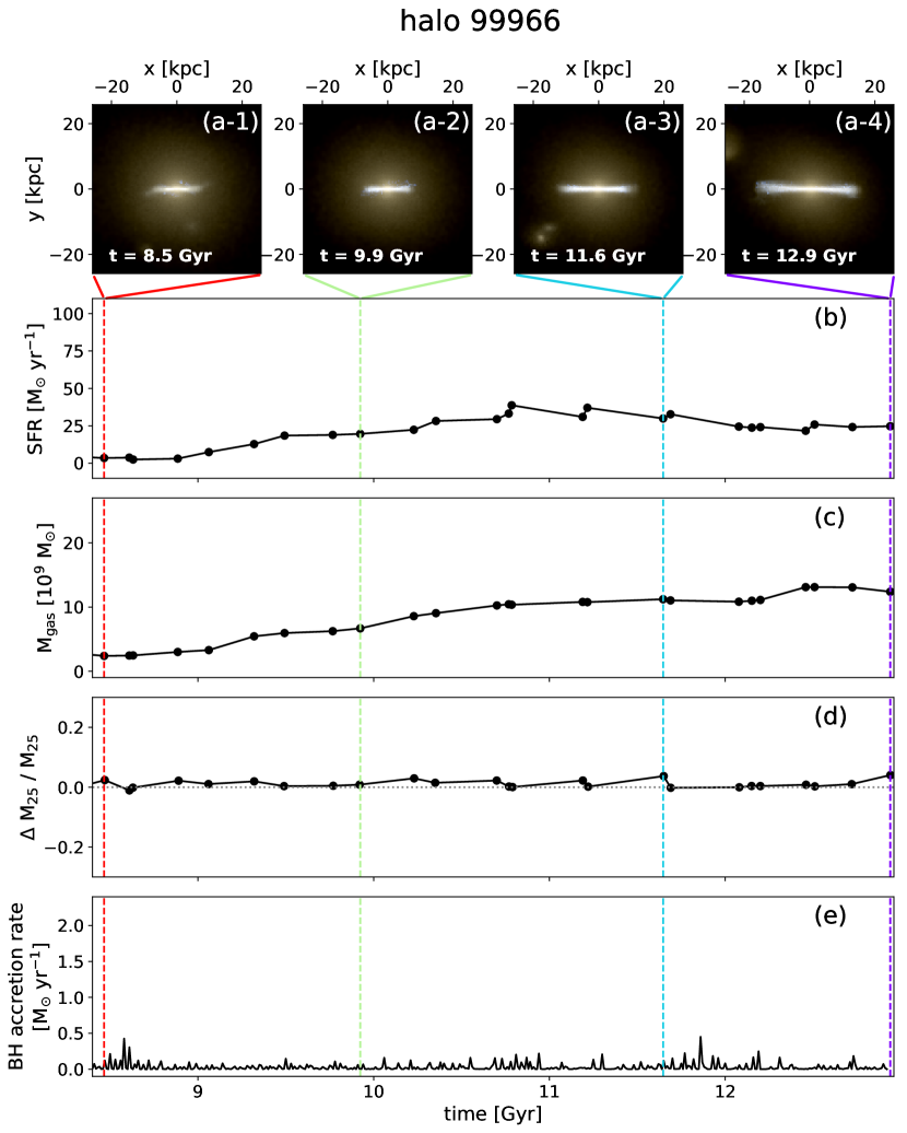
Figure 13: The recent evolution of the BGG of halo 99966. Panel (a-1 to -4): edge-on images of the galaxy at four selected epochs. Panel (b): the star formation rate measured within $50\,\rm kpc$ sphere centred at the halo. Panel (c): the cold gas mass measured within $50\,\rm kpc$ sphere centred at the halo. Panel (d): the variation of the total mass enclosed within a $25\,\rm kpc$ sphere ($\Delta M_{\rm 25}/M_{\rm 25}$) as a proxy for the mass accretion to the core (see text for details). The time frame of gravitational interactions with the BGG and satellites are coloured in pink. Panel (e): the black hole mass accretion rate.

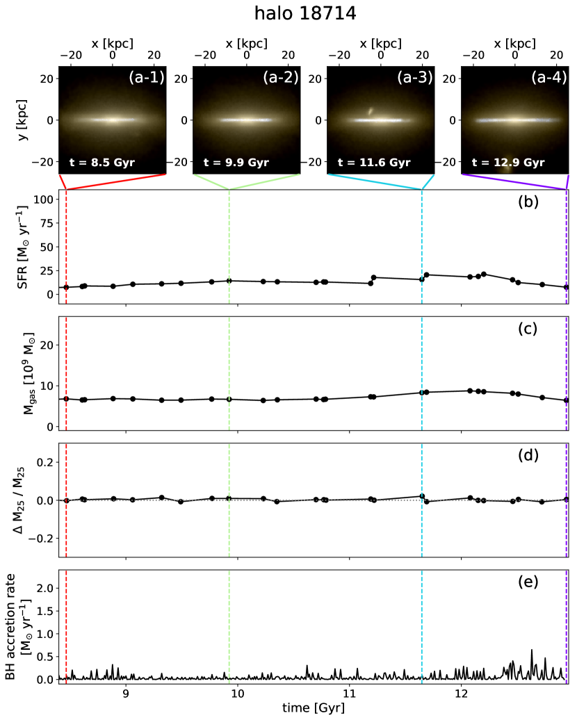
Figure 14: The same format as Fig. 13 for halo 18714.

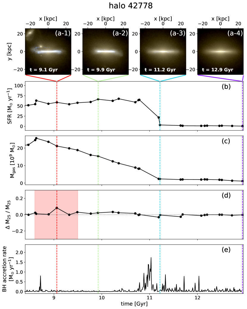
Figure 15: The same format as Fig. 13 for halo 42778.

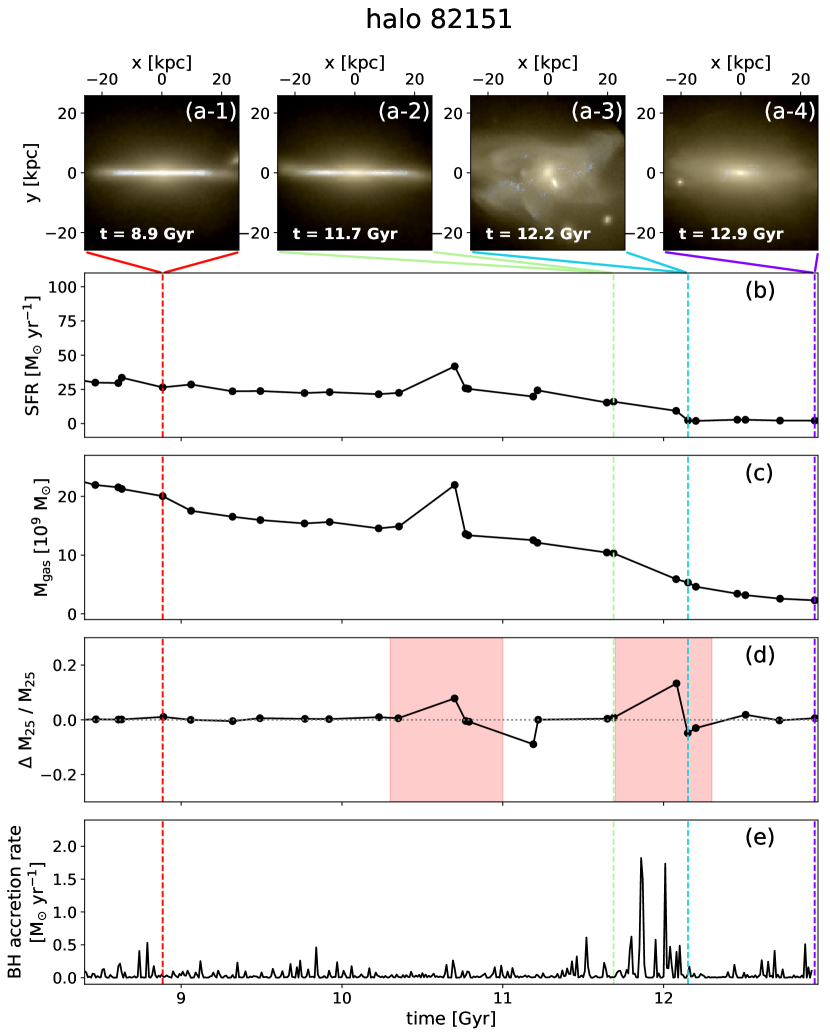
Figure 16: The same format as Fig. 13 for halo 82151.

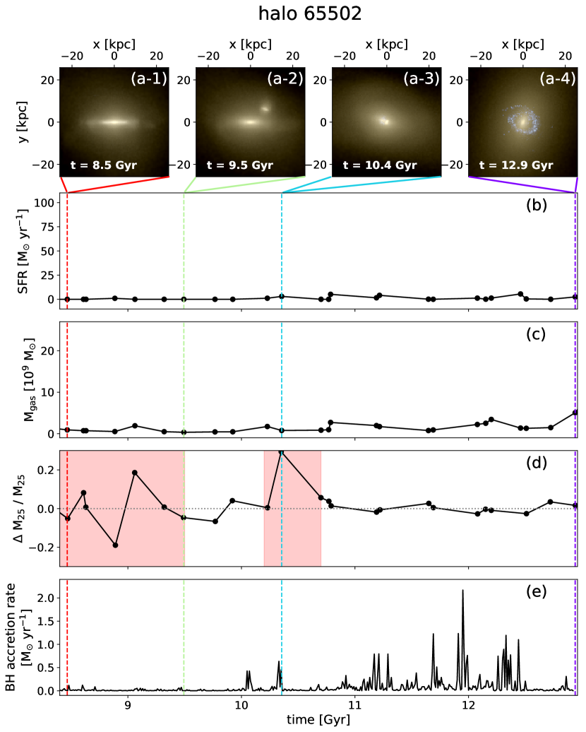
Figure 17: The same format as Fig. 13 for halo 65502.

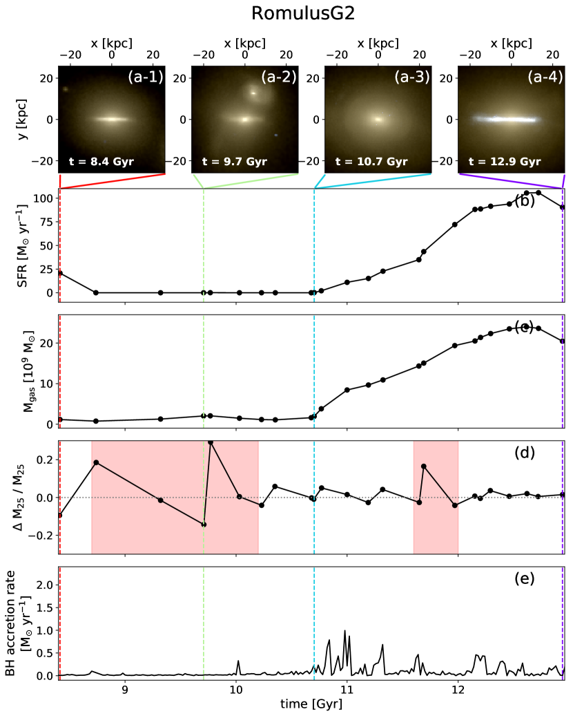
Figure 18: The same format as Fig. 13 for RomulusG2 halo.

4.3.1 Halo 99966

At $z=0.06$, the central BGG in group halo 99966 is a star forming ($SFR\approx 25\;{\rm M}_{\odot}\rm yr^{-1}$) disk galaxy (see panel a-4 of Fig. 13). The galaxy has not experienced any significant mergers or interactions with any subhalo or orbiting galaxy from 8.5 Gyrs onwards. However, both the BGG’s cold gas mass and the SFR steadily increase with time until $t\approx 11\,\rm Gyr$. The growth of the cold gas mass is due to the cooling of the CGM. After $t\approx 11\,\rm Gyr$, the gas mass more or less levels off while star formation starts to gently decrease. The modest SMBH activity between $t\approx 11.5-12\,\rm Gyr$ does not appear to be strong enough to impact the system.

4.3.2 Halo 18714

The BGG in halo 18714 is also a star forming disk galaxy at $z=0.06$. Like the previous example, this galaxy too has not experienced any significant gravitational encounter since 8.5 Gyrs. It has a stable cold gas mass until $t\approx 11.2\,\rm Gyr$; thereafter, the cold gas mass increases by $\Delta M_{\rm gas}\sim 2\times 10^{9}\,\rm M_{\odot}$ over $\sim$1 Gyr, and then slowly decreases. Prior to $t\approx 11.2\,\rm Gyr$, the SFR in this is rising gently. The increase in the cold gas mass edges the SFR a bit higher. This is followed by a downturn when the gas mass starts to decline. The increase in the cold gas mass is due to the cooling of the CGM. The turndown appears to be due to a more active SMBH from $t\approx 12\,\rm Gyr$ onwards.

4.3.3 Halo 42778

At $z=0.06$, the BGG of this halo has a large stellar disk (see panel a-4 of Fig. 15); however, its cold gas mass is low and on the basis of its SFR, the galaxy is quenched. Apart from what appears to be a minor interaction between $t=8.5$ and $9.5\,\rm Gyr$, this galaxy too has not suffered a disruptive merger/strong interaction event. Until $t\approx 11\,\rm Gyr$, the star formation is high and stable at $SFR\approx 60\;{\rm M}_{\odot}{\rm yr^{-1}}$ and there is no SMBH feedback activity to speak of. Over this same period, the cold gas mass starts out high ($M_{\rm gas}>2\times 10^{10}\,\rm M_{\odot}$) and decreases linearly with time until just after $t=11\,\rm Gyrs$, at which point it plateaus at $M_{\rm gas}{\;\raise 1.29167pt\hbox{$<$\kern-7.5pt\raise-4.73611pt\hbox{$\sim$}}\;}2\times 10^{9}\,\rm M_{\odot}$. The rate of decrease is too gentle given the SFR, suggesting a steady influx of gas from the CGM. At $t\approx 11\,\rm Gyr$, there is a sudden, extended period of powerful SMBH activity, followed by several slightly smaller outbursts extending for another $\sim 2$ Gyrs. The onset of this SMBH activity coincides with a steep plummeting of the SFR. With star formation nearly extinguished, the fact that the gas mass is not rising strongly suggests the influx of cooling CGM too has been quenched by SMBH activity. Why the SMBH suddenly turned on and why the outburst is so strong is a puzzle. We are looking into this as part of our forthcoming study.

4.3.4 Halo 82151

At $z=0.06$, this halo hosts a BGG that is the most massive of the early-type spheroidal Romulus galaxies. The star formation rate and the cold gas mass in this galaxy is steadily dropping with time, and at $z=0.06$, the galaxy is a quenched system. In panel (d) of Fig. 16, there are two peaks in $\Delta M_{\rm 25}/M_{\rm 25}$, at $t\approx 10.6\,\rm Gyr$ and $12\,\rm Gyr$, indicating that either the same satellite (over the course of its orbit) or two different satellites entered the 25 kpc sphere about the BGG. The first interaction has no apparent effect on the BGG. There is a brief increase in the star formation rate and cold gas mass at $t\approx 10.6\,\rm Gyr$, but this due to star formation and cold gas in a satellite entering the analysis sphere. The second interaction, however, is more impactful. It changes the BGG’s morphology, transforming it from a disk galaxy to a giant elliptical galaxy, and triggers a series of strong SMBH outburst, and quenches star formation.

4.3.5 Halo 65502

At $z=0.06$, the BGG of this halo has a ring of young, blue stars surrounded by extended diffuse stellar light composed of older stars (see panel a-4 of Fig. 17). At this time, the galaxy is still quenched but the star formation is rising and continues to rise to $z=0$. At $z=0$, the galaxy is classified as star forming. The ring of stars is an intriguing feature. As we had highlighted, the panels are oriented such that the total stellar angular momentum is orientated in the y-direction. The orbits of the young stars are not aligned with the bulk rotation of the old stars. The stars are forming in a settling stream. Panel (d) of Fig. 17 shows that the BGG has experienced two mergers/interactions, one stretching between $t=8.4$ and $9.5\,\rm Gyr$, and the other one at $t=10.2\,\rm Gyr$. During the first interaction, the satellite approaches and recedes a couple of times before merging. The resulting dynamical interactions transform the morphology of the BGG into a large spheroid. At this point, the galaxy’s star formation rate is low (quenched). Also, the SMBH is quiescent and the cold gas mass too is low. After the second interaction, galaxy receives two injections of a small amount of cold gas ($M_{\rm gas}\sim 10^{9}\,\rm M_{\odot}$). This period is also marked by strong episodic SMBH activity as well as bouts of slightly enhanced star formation (peak SFRs of $<5\,\rm M_{\odot}/yr$). The stream-like appearance of the stellar ring, its misaligned angular momentum and the prolonged yet intermittent bouts of SMBH and star formation activity all suggest that the second interloper was gas-rich and following a strong interaction, its response is similar to that seen in Poole et al. (2006) simulations: the galaxy’s gas is stretched out in a stream; bulk of the stream continues to orbit for a while although fragments occasionally detach and fall into the galaxy. Eventually, all of the gas ends up settling in the central galaxy, giving rise to the sharp rise in the cold gas mass (and eventually, star formation rate) towards the end. The delay of 1.5–2 Gyrs between the start of the satellite interaction and the eventual settling of the gas stream in the BGG is also consistent with the Poole et al. (2006) results.

4.3.6 RomulusG2

This BGG has an actively star-forming thin stellar disk embedded in a diffuse stellar halo at redshift $z=0.06$. The interaction history in Panel (d) shows multiple close encounters with satellites, with the first occurring between $t\approx 8.7$ and $10.2\,\rm Gyr$ (one of the passages is captured in the stellar map in panel a-2 of Fig. 18) while the second occurs at $11.8$ Gyrs. The first of these transforms the morphology of the BGG from a disk to a spheroid, with the galaxy resembling observed giant elliptical galaxies (panel a-3). There is no detectable star formation activity during this period and the cold gas mass too is low. However, about $\sim 1\,\rm Gyr$ after the last interaction with this first satellite, the cold gas mass and the star formation rate start to rise, growing linearly with time over the next 2 Gyrs and leading to the formation of a star forming disk embedded within the spheroidal distribution of older stars. The disk stands out in panel (a-4). This period also coincides with a prolonged period of modest SMBH activity but this activity appears to have no impact on the build up of the gas. Neither does the second interaction at 11.8 Gyrs. A cursory examination of the system suggests that the “rejuventation” of the BGG is due to slow settling of the gas stripped from the first satellite (Poole et al., 2006).

4.3.7 Summary from the case studies

We turned to these cases studies to get a better sense of why some galaxies end up as late type (star forming) systems and others as early type (quenched) systems. Following are some general observations:

• Star forming BGGs acquire their cold gas mass either from the cooling CGM or from settling streams of gas stripped from a gas rich satellite. Examples of the former include halos 99966 and 18714 while examples of the latter are halos 65502 and G2.

• In the case of late-type BGGs supported gas inflow from the CGM, in the absence of disruptive mergers, whether such systems remain star forming or quench depends to a large degree on whether the SMBH becomes active as well as on the strength of the bursts and the duration of the active period. Halos 99966 and 18714 are examples of systems where SMBH feedback has only little-to-no impact while halo 42778 is an example of a galaxy that experienced strong SMBH activity and ends up quenched.

• When star-forming disk BGGs are impacted by mergers/strong interactions, their star formation activity typically quenches and they are transformed into spheroids; see, for example, the transformation of halo 82151 at $t\approx 12\,\rm Gyr$. This process is often accompanied by strong SMBH activity and the cessation of gas flow from the CGM to the galaxy. At this stage, we cannot say whether the latter is the result of heating of the CGM due to merger-induced shocks, or the SMBH activity, or both acting in concert (e.g., Sanchez et al., 2021).

• In the case of galaxies that are already quenched but still flattened/disk-like, merger/interaction events also transform these galaxies into spheroidals. Whether the galaxies remain quenched spheroidals depends on whether the incoming secondary is gas-rich or not. The first interaction experienced by halo 65502 (at $t\approx 9.5\,\rm Gyr$) is an example of a transformation where the system remains quenched. The second interaction of halo 65502 and the evolution of RomulusG2 are examples where encounters with gas-rich satellites results in the “rejuvenation” of star formation in the BGGs. The onset of this rejuvenation can lag the initial satellite interaction by up to $\sim 2\,\rm Gyr$.

5 Conclusions

In this paper, we explored the properties of the massive galaxies in Romulus simulations at $z=0$. We specifically focused on the dominant central galaxies in group-scale halos (i.e., galaxies that are comparable to BGGs, the brightest group galaxies). This regime is often overlooked in galaxy demographic studies, compared to the Milky-way size galaxies or massive BCGs. The transition from blue, star-forming late-type galaxies to red, dead and round galaxies has often been attributed processes specific to cluster cores; however, our study shows that such transformations are common on the group-scale, a result will not be a surprise to those who study galaxy groups (see, for example, Sun et al., 2009; O’Sullivan et al., 2015; Liang et al., 2016; Oppenheimer et al., 2021; Lovisari et al., 2021a). BGGs are especially vulnerable to morphological transformations because the groups’ low-velocity dispersions make galaxy mergers/strong tidal interactions much more impactful. The presence of an extended CGM with short cooling time adds yet another dimension to the evolution of these systems.

There is also another reason for focusing on BGGs. Many of the current models of galaxy formation and evolution, including Romulus, are calibrated using measures that are strongly influenced by the properties and evolution of “normal” Milky Way-like ($\sim L*$; $\sim M*$) galaxies. Since these galaxies populate the knee of the galaxy luminosity/stellar mass functions (Schechter, 1976), they dominate the integrated cosmic mass and luminosity densities at low redshift, and also numerically dominate the flux-limited surveys at moderate redshifts. By virtue of being more massive systems residing in very different, typically more gas rich, environments than Milky Way-like systems, and subject to very different evolutionary processes, BGGs offer an opportunity to stress-test the galaxy formation models.

We compared the stellar masses, the kinematic properties, the morphologies, and the star formation rates of the Romulus BGGs against observations. We find that on the whole the properties of the BGGs in low mass groups (i.e., $\rm M_{\rm 200}{\;\raise 1.29167pt\hbox{$<$\kern-7.5pt\raise-4.73611pt\hbox{$\sim$}}\;}10^{13}\;\rm M_{\odot}$) are in excellent agreement with the observations. We find both early-type S0 and elliptical galaxies as well as late-type disk galaxies at the centers of Romulus low-mass groups, in agreement with the results of Weinmann et al. (2006) and Olivares et al. (2021); we find Romulus galaxies that are fast rotators as well as slow rotators; and we observe galaxies transforming from late-type to early-type following strong dynamical interactions with orbiting/merging satellites.

There are, however, signs that Romulus simulations are straining in the regime of massive (rich) groups, with some of the properties of the corresponding BGGs increasingly at odds with the observations. The most important of these are (i) a rising, instead of decreasing, fraction of late-type BGGs with halo mass, and (ii) a higher than observed star formation rates in some of the galaxies.

Examining a few galaxies more carefully, to get a better sense of how BGGs evolve into and express diverse characteristics, we find that their evolution is governed by competition between influx of cool gas from the CGM, gas brought in by satellites, SMBH outbursts, as well as shock heating and galaxy transformation due to orbiting/merging satellites. The importance of each of these varies from system to system, which in turn gives rise to a wide range of evolutionary pathways. In high mass groups, however, we noted a preponderance of “rejuvenated” galaxies; that is, BGGs that initially transform into quenched spheroidal galaxies but which subsequently receive an influx of gas and are able to re-grow a star forming disk at late times. This is especially noticeable on mass scale $\rm M_{\rm 200}>10^{13}\;\rm M_{\odot}$.

One can ask whether this could be due to the exclusion of high-temperature (i.e. $T>10^{4}\,\rm K$) metal-line cooling in Romulus simulations. At first glance, this seems unlikely. The inclusion of metal cooling will, in the first instance, enhance cooling and ought to exacerbate the problem. In practice, as discussed in detail in Section 2.1, most existing galaxy formation simulations that include metal cooling have the opposite problem in that the IGrM gas is in fact overheated and the resulting IGrM entropy profiles do not agree with those inferred from observations. We speculate that both problems, the decreasing effectiveness of SMBH feedback in Romulus with increasing halo mass on the group/cluster scale, and the over-aggressive SMBH feedback responses that overheat the IGrM in simulations like EAGLE, SIMBA and IllustrisTNG, all signal the failure of the current ad hoc sub-grid prescriptions and numerical implementations for SMBH accretion and feedback. Collectively these challenges spotlight the critical need to revisit and improve the current SMBH model and possibly even, its implementation.

Data availability

The data directly related this article will be shared on reasonable request to the corresponding author. Galaxy database & particle data for Romulus is available upon request from Michael Tremmel.

Appendix A Observed parameters

A.1 Stellar mass

Table 3: The stellar mass measuring methods of the observation references presented in Fig. 1

	Data	Method
Yang et al. (2008)	SDSS DR4 (NYU-VAGC)	Photometric. Petrosian r-band magnitude within the Petrosian radius is converted to the stellar mass based on the M/L from the SPS model of Bell et al. (2003) assuming ‘diet’ Salpeter IMF.
Yang et al. (2012)	SDSS DR7	Photometric. Similar to Yang et al. (2008), using Kroupa (2002) IMF.
Moster et al. (2013)	SDSS DR7	Photometric. Model r-band magnitude is converted to the stellar mass using Li & White (2009) stellar mass measurements and the M/L from the SPS model of Blanton & Roweis (2007) assuming Chabrier IMF. SDSS model magnitude is calculated by fitting a surface brightness profile to the exponential or the de Vacoulers profile, whichever better, and integrating it to the infinite radius. It is a better estimate of the total mass of galaxies than Petrosian magnitudes.
Kravtsov et al. (2018)	SDSS DR8	Photometric. Extended luminosity profiles are constructed by fitting a triple-Sérsic profile and then integrated out to $50\,\rm kpc$ or the infinite radius. The luminosity is converted to the stellar mass based on the M/L from the SPS model of Bell et al. (2003) and then adjusted to emulate Chabrier IMF.
L18	2MASS	Photometric. Total K-band magnitude is calculated by fitting a single-Sérsic profile and integrating it to the infinite radius. The luminosity is then converted to the stellar mass based on the M/L from the dynamical modelling of Cappellari (2013).
van Uitert et al. (2018)	GAMA	SPS modelling. SED templates are built based on $ugriz$- and NIR-magnitude scaled to cover 10 effective radius of the galaxies. SED fitting is performed using the SPS model by Bruzual & Charlot (2003) assuming an exponential star formation history and Chabrier IMF.
Erfanianfar et al. (2019)	GALEX SDSS DR14 WISE	SPS modelling. Observed SEDs are constructed based on UV, optical ($ugriz$-cModel magnitude), and IR data. SDSS cModel magnitude is calculated by fitting a surface brightness profile to a linear combination of the exponential and the de Vacoulers profile and integrating to infinite radius. SED templates are built using the SPS model by Bruzual & Charlot (2003) assuming exponential star formation history and Chabrier IMF.
Girelli et al. (2020)	SDSS DR4 (NYU-VAGC)	Combination of photometric and SPS modelling. Baldry et al. (2008) calculate the weighted-average of four independent stellar mass measures using NYU-VAGC Petrosian $ugriz$-magnitude, spectral features (e.g., D4000, H$\rm\delta$), PEGASE SPS models (Fioc & Rocca-Volmerange 1997), and Bruzual & Charlot (2003) SPS models. Then the results are rescaled to follow Planck 2015 cosmology and Chabrier IMF.

Table 4: The stellar mass measuring methods of the observation references presented in Fig. 10

	Data	Method
Whitaker et al. (2012)	NMBS	SPS modelling. SED templates are built using the SPS model by Bruzual & Charlot (2003) assuming an exponential star formation history, solar metallicity, and Chabrier IMF. Dust extinction is taken into account following Calzetti et al. (2000).
Mittal et al. (2015)	GALEX 2MASS HST optical SDSS DR10	SPS modelling. SEDs are constructed based on multi-wavelength data from UV to IR. The aperture size is provided in tables in the paper in arcsec unit. SED fitting is performed using GALAXEV (Bruzual & Charlot 2003) assuming Chabrier IMF.
Gozaliasl et al. (2016)	COSMOS CFHTLS	SPS modelling. SEDs are constructed based on ugriz-magnitudes. SED template fitting is performed using LE PHARE code (Arnouts et al. 1999; Ilbert et al. 2006) and FAST code (Kriek et al. 2009) with Bruzual & Charlot (2003) SSP and Chabrier IMF.
Cooke et al. (2018)	GALEX Subaru optical Vista Herschel	SPS modelling SEDs are constructed based on multi-wavelength data from FUV to FIR. SED fitting is performed using Bruzual & Charlot (2003) SSP and Chabrier IMF.

Converting observed photometric/spectroscopic properties to the stellar mass is based on the stellar population synthesis modeling. Table 3 and Table 4 summarizes different stellar mass measurements in observation studies presented in Fig. 1 and Fig. 10, respectively. Among the literatures, van Uitert et al. (2018), Erfanianfar et al. (2019), Whitaker et al. (2012), Mittal et al. (2015), Gozaliasl et al. (2016), and Cooke et al. (2018) performed a direct SPS modeling; they constructed spectral energy distributions (SEDs) of galaxies based on multi-wavelength data and searched for a set of stellar populations that best fits the observed spectra/magnitudes. Alternatively, one can adopt the stellar mass-to-light ratio (M/L) estimated based on the properties that are well-known to correlate with M/L. In Fig. 1, Yang et al. (2008); Yang et al. (2012), Kravtsov et al. (2018), and Girelli et al. (2020) utilized a correlation between a photometric colour and M/L from Bell et al. (2003). Similarly, Moster et al. (2013) adopted M/L from Blanton & Roweis (2007) stellar population models. L18 used M/L from Cappellari (2013); in contrast to the former mentioned M/L references, Cappellari (2013) estimated the M/L from the 3D kinematic modeling of early-type galaxies, therefore, the stellar mass corresponds to the dynamical mass.

The stellar mass measure based on the photometry and the population synthesis modeling depends on a number of factors, such as which initial mass function (IMF) is assumed, how well the stellar mass-to-light ratio is constrained (see Loubser et al., 2021, and references therein), and how far from the center the stellar light is mapped (Gonzalez et al., 2013; Kravtsov et al., 2018; DeMaio et al., 2020). The latter is a particularly vexing issue. Typically, the stellar light associated with a BGG/BCG extends smoothly out from the group/cluster center. Although this distribution is conventionally referred to as BCG+ICL (or BGG+IGrL), there is no clear break or edge to indicate where the galactic stellar component ends and the intragroup/intracluster light (IGrL/ICL) begins (see, e.g., Contini 2021; Contini et al. 2022). For this reason, most studies do not attempt to distinguish between the two. With increasing distance from the center, the surface brightness profile drops and eventually fade into the sky background (DeMaio et al., 2020). The over-subtraction of the sky background light is one of the main causes of the underestimated stellar mass (e.g., Von Der Linden et al. 2007; Bernardi et al. 2007; He et al. 2013). There have been several studies showing that the estimated BGG & BCG  stellar masses from SDSS photometry have been systematically underestimated and that the bias becomes more severe with increasing mass (Hill et al. 2011; Simard et al. 2011; Bernardi et al. 2013; Gonzalez et al. 2013; Kravtsov et al. 2018). For example, Kravtsov et al. (2018) reported an increased stellar mass at the high-mass end of the SMHM relation when a careful treatment of background subtraction was applied.

A.2 Halo mass

Table 5: The halo mass measuring methods of the observation references presented in Fig. 1

	Data	Method
Yang et al. (2008)	Halo mass function from Warren et al. (2006) assuming WMAP3 cosmology	Abundance matching. The ranking is based on (i) the total luminosity or (ii) the total stellar mass of a galaxy group.
Yang et al. (2012)	Halo mass function from Warren et al. (2006) assuming WMAP7 cosmology	Abundance matching. Similar to Yang et al. (2008), with improved treatments on subhalos.
Moster et al. (2013)	Halo catalogues from Millenium & Millenium-II simulations converted to WMAP7 cosmology	Abundance matching.
Kravtsov et al. (2018)	Chandra X-ray data	X-ray observations. $Y_{X}\equiv M_{g}T_{X}$ is converted to the halo mass (see Kravtsov et al. 2006 for details).
L18	Chandra X-ray data XMM-Newton X-ray data Weak lensing data in optical	For the CLoGS sample, X-ray system temperature $T_{\rm sys}$ is converted to the halo mass based on the scaling relations from Sun et al. (2009). For the MENeaCS and the CCCP sample, weak lensing analysis is used (Herbonnet et al. 2017; Hoekstra et al. 2015).
van Uitert et al. (2018)	KiDS survey	Weak lensing analysis.
Erfanianfar et al. (2019)	SPIDERS-CODEX XMM-Newton XMM-CFHTLSXMM-XXL	X-ray luminosity $L_{X}$ is converted to the halo mass based on the redshift dependent scaling relations from Leauthaud et al. (2010).
Girelli et al. (2020)	Halo catalogues from the $\Lambda$CDM DUSTGRAIN-pathfinder simulation based on Planck 2015 cosmology.	Abundance matching.

Table 5 summarizes how the galaxies’ host halo mass is measured in observation studies presented in Fig. 1. One of the methods to derive the halo mass from observables is to use X-ray observations assuming the X-ray emitting gas is in hydrostatic equilibrium within the group/cluster potential. In Fig. 1, Kravtsov et al. (2018), L18 BGGs, and Erfanianfar et al. (2019) used this approach. Although the mass estimate resulting from this method has been shown to be systematically biased (Mahdavi et al., 2013), the approach works well for clusters and massive groups once the bias is accounted for. To correct the bias, we scaled the halo mass of all the X-ray observation results by 1.25 when presenting them in Fig. 1. However, this method cannot, as of yet, be straightforwardly applied to low-mass groups, because a significant fraction of such systems tend to be X-ray under-luminous (Pearson et al., 2017; O’Sullivan et al., 2017) and as a result do not have extended X-ray observations on which to base the mass estimate. This brings up concerns that systems which are X-ray bright might not be representative of the population as a whole.

Alternatively, L18 BCGs and van Uitert et al. (2018) in Fig. 1 estimated the halo masses using the weak gravitational lensing analysis. In terms of reliably estimating the mass of an individual system, the approach works best for massive clusters. Even then, the uncertainties in mass estimates for individual systems is $\sim 15-25\%$ (Hoekstra et al. 2015) and these uncertainties grow with decreasing halo masses.

For this reason, halo masses of lower mass systems are frequently estimated using indirect methods that relate observed galaxies to their host halos. In Fig. 1, Yang et al. (2008); Yang et al. (2012), Moster et al. (2013), and Girelli et al. (2020) used this approach. One such method, the halo abundance matching establishes a connection between observed galaxies and the halo mass function predicted from analytic models or N-body simulations. Essentially, more luminous galaxies are assigned to more massive halos. There are more sophisticated approaches, such as halo occupation distribution (e.g., Berlind & Weinberg 2002; Cooray & Sheth 2002; Tinker et al. 2005) and conditional luminosity/stellar mass function (e.g., Yang et al. 2003; Cooray 2006), that construct the connection between galaxies and halos using the number of galaxies and the galaxy luminosity function in a given halo mass, respectively. It is worth pointing out that the halo mass function is dependent on cosmology. As a result, the halo mass assigned to galaxies via abundance matching is subject to change depending on the choice of cosmology. When comparing WMAP7 and Planck cosmology, Rodríguez-Puebla et al. (2016) showed that their simulation based on Planck cosmology resulted in slightly higher abundance of massive halos compared to the one based on WMAP7. However, the variation in the SMHM relation is relatively small among cosmology models, therefore, we omit the conversion between cosmologies when comparing results presented in Fig. 1. Similarly in Yang et al. (2012), the authors compared the SMHM relations derived from different cosmology models, namely, WMAP1, WMAP3, WMAP5, and WMAP7. The differences in the resulting SMHM relations due to cosmology are minor compared to the collective scatter in a compilation of SMHM relations (see, for example, Fig. 10 of Coupon et al. 2015 or Fig. 9 of Girelli et al. 2020.

The above references refer to several different definitions of the halo mass, e.g., $M_{\rm 200}$, $M_{\rm 500}$. Conventionally, the subscript denotes the overdensity ($\Delta$) and $M_{\rm\Delta}$ and $R_{\rm\Delta}$ are the mass and radius of a sphere with the enclosed mass density equals to $\Delta$ times the critical density ($\rho_{\rm crit}$):

$$M_{\Delta}(r<R_{\Delta})=\frac{4}{3}\pi R_{\Delta}^{3}\Delta\rho_{\rm crit}.$$ (2)

For a fair comparison between the results, we mapped the halo masses to $M_{\rm 200}$, following the procedure described here. First, we calculated the exact conversion factor that converts $M_{\rm\Delta_{1}}$ to $M_{\rm\Delta_{2}}$, where $\Delta_{1}$ is the choice of overdensity in a literature and $\Delta_{2}=200$ in our case. When assuming an NFW profile, the radial density distribution of a system can be characterized by the scale density $\rho_{0}$, the scale radius $r_{s}$, and the mass enclosed within $R_{\rm\Delta}$. These are related as follows:

$$M_{\rm\Delta}=4\pi\rho_{\rm 0}r_{\rm s}^{3}m(c_{\rm\Delta}),$$ (3)

where $c_{\rm\Delta}\equiv R_{\rm\Delta}/r_{s}$ is a concentration parameter and $m(x)=\ln(1+x)-x/(1+x)$. Combining equation (2) and equation (3), we get the following relation between the two definitions of halo mass.

$$\begin{cases}\frac{M_{\rm\Delta_{2}}}{M_{\rm\Delta_{1}}}=\left(\frac{c_{\rm\Delta_{2}}}{c_{\rm\Delta_{1}}}\right)^{3}\frac{\Delta_{2}}{\Delta_{1}}\\ \frac{c_{\rm\Delta_{2}}}{c_{\rm\Delta_{1}}}=\left[\frac{\Delta_{1}}{\Delta_{2}}\frac{m(c_{\rm\Delta_{2}})}{m(c_{\rm\Delta_{1}})}\right]^{\frac{1}{3}}.\end{cases}$$ (4)

Dutton & Macciò (2014) have shown that mass and concentration parameters are tightly correlated. For the halo mass range of interest to us, we noticed that the conversion factor ($M_{\Delta_{2}}/M_{200}$) correlates almost linearly with mass in log scale. Therefore, we derived a linear conversion and used this relation to scale a given halo mass to $M_{200}$.

A.3 Star formation rate

Table 6: The SFR measuring methods of the observation references presented in Fig. 10

	Data	Method
Whitaker et al. (2012)	NMBS	UV and IR luminosities are converted to SFR using the relation from Kennicutt (1998) (${SFR}_{\rm UV+IR}=0.98\times 10^{-10}(L_{\rm IR}+3.3L_{\rm 2800})$) assuming Kroupa IMF. The star-forming galaxies are selected based on $U-V$ and $V-J$ colours.
Mittal et al. (2015)	GALEX 2MASS HST optical SDSS DR10	SFR is computed from SED constructed based on multi-wavelength data from UV to IR. SED fitting is performed using GALAXEV code (Bruzual & Charlot 2003) assuming Chabrier IMF.
Gozaliasl et al. (2016)	COSMOS CFHTLS	SFR is computed from SED constructed based on ugriz-magnitudes. SED template fitting is performed using LE PHARE code (Arnouts et al. 1999; Ilbert et al. 2006) and FAST code (Kriek et al. 2009) with Bruzual & Charlot (2003) SSP and Chabrier IMF.
L18	GALEX 2MASS/MIPS IRAM 30m	SFR is the sum of the UV- and IR-based SFRs measured separately. For the BCGs, SFR is from Hoffer et al. (2012). For the BGGs, IR-based SFR is from O’Sullivan et al. (2015); O’Sullivan et al. (2018) and UV-based SFR is from Kolokythas et al. (2021).
Cooke et al. (2018)	GALEX Subaru optical Vista Herschel	SFR is computed from SED constructed based on multi-wavelength data from UV to IR. SED fitting is performed using iSEDfit code (Moustakas et al., 2013; Moustakas, 2017) and Bruzual & Charlot (2003) SSP templates assuming Salpeter IMF

Table 6 summarizes how the star formation rate is measured in observations presented in Fig. 10. The star formation rate estimations of Whitaker et al. (2012), Mittal et al. (2015), Gozaliasl et al. (2016), and Cooke et al. (2018) are based on SEDs constructed using infrared and/or optical magnitudes. The star formation rate of L18 BCGs are from Hoffer et al. (2012). Similarly for L18 BGGs, we take the total SFR to be the sum of the obscured and unobscured SFR (i.e., IR-based star formation rates from O’Sullivan et al. 2015; O’Sullivan et al. 2018 and UV-based star formation rates from Kolokythas et al. 2021); many of these galaxies are lacking IR observations and consequently, their SFRs are strictly speaking, lower limits.

References

- Abadi et al. (2003) Abadi M. G., Navarro J. F., Steinmetz M., Eke V. R., 2003, ApJ, 597, 21
- Arnouts et al. (1999) Arnouts S., Cristiani S., Moscardini L., Matarrese S., Lucchin F., Fontana A., Giallongo E., 1999, MNRAS, 310, 540
- Babul et al. (2002) Babul A., Balogh M. L., Lewis G. F., Poole G. B., 2002, MNRAS, 330, 329
- Babul et al. (2013) Babul A., Sharma P., Reynolds C. S., 2013, ApJ, 768, 11
- Bahé et al. (2017) Bahé Y. M., et al., 2017, MNRAS, 470, 4186
- Baldry et al. (2008) Baldry I. K., Glazebrook K., Driver S. P., 2008, MNRAS, 388, 945
- Balogh et al. (1999) Balogh M. L., Babul A., Patton D. R., 1999, MNRAS, 307, 463
- Barnes et al. (2017) Barnes D. J., Kay S. T., Henson M. A., McCarthy I. G., Schaye J., Jenkins A., 2017, MNRAS, 465, 213
- Bassini et al. (2020) Bassini L., et al., 2020, A&A, 642, A37
- Bell et al. (2003) Bell E. F., McIntosh D. H., Katz N., Weinberg M. D., 2003, ApJS, 149, 289
- Bellovary et al. (2014) Bellovary J. M., Holley-Bockelmann K., Gültekin K., Christensen C. R., Governato F., Brooks A. M., Loebman S., Munshi F., 2014, MNRAS, 445, 2667
- Bender et al. (2015) Bender R., Kormendy J., Cornell M. E., Fisher D. B., 2015, ApJ, 807, 56
- Benson et al. (2007) Benson A. J., Džanović D., Frenk C. S., Sharples R., 2007, MNRAS, 379, 841
- Berlind & Weinberg (2002) Berlind A. A., Weinberg D. H., 2002, ApJ, 575, 587
- Bernardi et al. (2007) Bernardi M., Hyde J. B., Sheth R. K., Miller C. J., Nichol R. C., 2007, AJ, 133, 1741
- Bernardi et al. (2013) Bernardi M., Meert A., Sheth R. K., Vikram V., Huertas-Company M., Mei S., Shankar F., 2013, MNRAS, 436, 697
- Bildfell et al. (2008) Bildfell C., Hoekstra H., Babul A., Mahdavi A., 2008, MNRAS, 389, 1637
- Binney (1978) Binney J., 1978, MNRAS, 183, 501
- Binney (2005) Binney J., 2005, MNRAS, 363, 937
- Binney & Tabor (1995) Binney J., Tabor G., 1995, MNRAS, 276, 663
- Blanton & Roweis (2007) Blanton M. R., Roweis S., 2007, AJ, 133, 734
- Blanton et al. (2005) Blanton M. R., et al., 2005, AJ, 129, 2562
- Bottrell et al. (2017) Bottrell C., Torrey P., Simard L., Ellison S. L., 2017, MNRAS, 467, 2879
- Boylan-Kolchin et al. (2009) Boylan-Kolchin M., Springel V., White S. D. M., Jenkins A., Lemson G., 2009, MNRAS, 398, 1150
- Brinchmann et al. (2004) Brinchmann J., Charlot S., White S. D. M., Tremonti C., Kauffmann G., Heckman T., Brinkmann J., 2004, MNRAS, 351, 1151
- Brough et al. (2005) Brough S., Collins C. A., Burke D. J., Lynam P. D., Mann R. G., 2005, MNRAS, 364, 1354
- Brough et al. (2008) Brough S., Couch W. J., Collins C. A., Jarrett T., Burke D. J., Mann R. G., 2008, MNRAS, 385, L103
- Bruzual & Charlot (2003) Bruzual G., Charlot S., 2003, MNRAS, 344, 1000
- Bullock & Johnston (2005) Bullock J. S., Johnston K. V., 2005, ApJ, 635, 931
- Butsky et al. (2019) Butsky I. S., Burchett J. N., Nagai D., Tremmel M., Quinn T. R., Werk J. K., 2019, MNRAS, 490, 4292
- Calzetti et al. (2000) Calzetti D., Armus L., Bohlin R. C., Kinney A. L., Koornneef J., Storchi-Bergmann T., 2000, ApJ, 533, 682
- Cappellari (2008) Cappellari M., 2008, MNRAS, 390, 71
- Cappellari (2013) Cappellari M., 2013, ApJ, 778, L2
- Cappellari et al. (2006) Cappellari M., et al., 2006, MNRAS, 366, 1126
- Cappellari et al. (2011) Cappellari M., et al., 2011, MNRAS, 413, 813
- Cappellari et al. (2013) Cappellari M., et al., 2013, MNRAS, 432, 1709
- Carter et al. (1999) Carter D., Bridges T. J., Hau G. K. T., 1999, MNRAS, 307, 131
- Chadayammuri et al. (2021) Chadayammuri U., Tremmel M., Nagai D., Babul A., Quinn T., 2021, MNRAS, 504, 3922
- Christensen et al. (2014) Christensen C. R., Governato F., Quinn T., Brooks A. M., Shen S., McCleary J., Fisher D. B., Wadsley J., 2014, MNRAS, 440, 2843
- Cielo et al. (2018) Cielo S., Babul A., Antonuccio-Delogu V., Silk J., Volonteri M., 2018, Astronomy & Astrophysics, 617, A58
- Ciotti & Ostriker (2001) Ciotti L., Ostriker J. P., 2001, ApJ, 551, 131
- Clauwens et al. (2018) Clauwens B., Schaye J., Franx M., Bower R. G., 2018, MNRAS, 478, 3994
- Colless et al. (2001) Colless M., et al., 2001, MNRAS, 328, 1039
- Conroy et al. (2007) Conroy C., Wechsler R. H., Kravtsov A. V., 2007, ApJ, 668, 826
- Conselice (2006) Conselice C. J., 2006, MNRAS, 373, 1389
- Contini (2021) Contini E., 2021, Galaxies, 9, 60
- Contini et al. (2022) Contini E., Chen H. Z., Gu Q. S., 2022, arXiv e-prints, p. arXiv:2202.10675
- Cooke et al. (2018) Cooke K. C., Fogarty K., Kartaltepe J. S., Moustakas J., O’Dea C. P., Postman M., 2018, ApJ, 857, 122
- Cooray (2006) Cooray A., 2006, MNRAS, 365, 842
- Cooray & Sheth (2002) Cooray A., Sheth R., 2002, Phys. Rep., 372, 1
- Correa et al. (2017) Correa C. A., Schaye J., Clauwens B., Bower R. G., Crain R. A., Schaller M., Theuns T., Thob A. C. R., 2017, MNRAS, 472, L45
- Cougo et al. (2020) Cougo J., Rembold S. B., Ferrari F., Kaipper A. L. P., 2020, MNRAS, 498, 4433
- Coupon et al. (2015) Coupon J., et al., 2015, MNRAS, 449, 1352
- Crain et al. (2015) Crain R. A., et al., 2015, MNRAS, 450, 1937
- Cui et al. (2018) Cui W., et al., 2018, MNRAS, 480, 2898
- Cui et al. (2022) Cui W., et al., 2022, arXiv e-prints, p. arXiv:2202.14038
- Davé et al. (2008) Davé R., Oppenheimer B. D., Sivanandam S., 2008, MNRAS, 391, 110
- Davé et al. (2019) Davé R., Anglés-Alcázar D., Narayanan D., Li Q., Rafieferantsoa M. H., Appleby S., 2019, MNRAS, 486, 2827
- Davé et al. (2020) Davé R., Crain R. A., Stevens A. R. H., Narayanan D., Saintonge A., Catinella B., Cortese L., 2020, MNRAS, 497, 146
- Davison et al. (2020) Davison T. A., Norris M. A., Pfeffer J. L., Davies J. J., Crain R. A., 2020, MNRAS, 497, 81
- De Lucia & Blaizot (2007) De Lucia G., Blaizot J., 2007, MNRAS, 375, 2
- DeMaio et al. (2020) DeMaio T., et al., 2020, MNRAS, 491, 3751
- Deeley et al. (2017) Deeley S., et al., 2017, MNRAS, 467, 3934
- Dominguez Romero et al. (2012) Dominguez Romero M. J. d. L., Garcia Lambas D., Muriel H., 2012, MNRAS: Letters, 427, L6
- Dressler (1979) Dressler A., 1979, ApJ, 231, 659
- Driver et al. (2006) Driver S. P., et al., 2006, MNRAS, 368, 414
- Driver et al. (2011) Driver S. P., et al., 2011, MNRAS, 413, 971
- Duarte & Mamon (2015) Duarte M., Mamon G. A., 2015, MNRAS, 453, 3848
- Dubinski (1998) Dubinski J., 1998, ApJ, 502, 141
- Dubois et al. (2011) Dubois Y., Devriendt J., Teyssier R., Slyz A., 2011, MNRAS, 417, 1853
- Dubois et al. (2016) Dubois Y., Peirani S., Pichon C., Devriendt J., Gavazzi R., Welker C., Volonteri M., 2016, MNRAS, 463, 3948
- Dutton & Macciò (2014) Dutton A. A., Macciò A. V., 2014, MNRAS, 441, 3359
- Eke et al. (2004) Eke V. R., et al., 2004, MNRAS, 355, 769
- Elbaz et al. (2011) Elbaz D., et al., 2011, A&A, 533, A119
- Emsellem et al. (2011) Emsellem E., et al., 2011, MNRAS, 414, 888
- Erfanianfar et al. (2019) Erfanianfar G., et al., 2019, A&A, 631, A175
- Faber & Jackson (1976) Faber S. M., Jackson R. E., 1976, ApJ, 204, 668
- Finoguenov et al. (2007) Finoguenov A., et al., 2007, ApJS, 172, 182
- Fioc & Rocca-Volmerange (1997) Fioc M., Rocca-Volmerange B., 1997, A&A, 500, 507
- Fisher et al. (1995) Fisher D., Illingworth G., Franx M., 1995, ApJ, 438, 539
- Freeman (1970) Freeman K. C., 1970, ApJ, 160, 811
- Furnell et al. (2018) Furnell K. E., et al., 2018, MNRAS, 478, 4952
- Girardi et al. (2010) Girardi L., et al., 2010, ApJ, 724, 1030
- Girelli et al. (2020) Girelli G., Pozzetti L., Bolzonella M., Giocoli C., Marulli F., Baldi M., 2020, A&A, 634, A135
- Gonzalez et al. (2013) Gonzalez A. H., Sivanandam S., Zabludoff A. I., Zaritsky D., 2013, ApJ, 778, 14
- Gozaliasl et al. (2016) Gozaliasl G., Finoguenov A., Khosroshahi H. G., Mirkazemi M., Erfanianfar G., Tanaka M., 2016, MNRAS, 458, 2762
- Groenewald et al. (2017) Groenewald D. N., Skelton R. E., Gilbank D. G., Loubser S. I., 2017, MNRAS, 467, 4101
- Harris et al. (2020) Harris C. R., et al., 2020, Nature, 585, 357–362
- He et al. (2013) He Y. Q., Xia X. Y., Hao C. N., Jing Y. P., Mao S., Li C., 2013, ApJ, 773, 37
- Helsdon & Ponman (2003) Helsdon S. F., Ponman T. J., 2003, MNRAS, 340, 485
- Henden et al. (2018) Henden N. A., Puchwein E., Shen S., Sijacki D., 2018, MNRAS, 479, 5385
- Henden et al. (2020) Henden N. A., Puchwein E., Sijacki D., 2020, MNRAS, 498, 2114
- Herbonnet et al. (2017) Herbonnet R., Buddendiek A., Kuijken K., 2017, A&A, 599, A73
- Herbonnet et al. (2020) Herbonnet R., et al., 2020, MNRAS, 497, 4684
- Hill et al. (2011) Hill D. T., et al., 2011, MNRAS, 412, 765
- Hoekstra et al. (2015) Hoekstra H., Herbonnet R., Muzzin A., Babul A., Mahdavi A., Viola M., Cacciato M., 2015, MNRAS, 449, 685
- Hoffer et al. (2012) Hoffer A. S., Donahue M., Hicks A., Barthelemy R. S., 2012, ApJS, 199, 23
- Hunter (2007) Hunter J. D., 2007, Computing in Science and Engineering, 9, 90
- Ilbert et al. (2006) Ilbert O., et al., 2006, A&A, 457, 841
- Ilbert et al. (2010) Ilbert O., et al., 2010, ApJ, 709, 644
- Ilbert et al. (2015) Ilbert O., et al., 2015, A&A, 579, A2
- Jackson et al. (2020) Jackson T. M., Pasquali A., Pacifici C., Engler C., Pillepich A., Grebel E. K., 2020, MNRAS, 497, 4262
- Jarrett et al. (2003) Jarrett T. H., Chester T., Cutri R., Schneider S. E., Huchra J. P., 2003, AJ, 125, 525
- Jeans (1922) Jeans J. H., 1922, MNRAS, 82, 122
- Jian et al. (2014) Jian H.-Y., et al., 2014, ApJ, 788, 109
- Johnston et al. (2008) Johnston K. V., Bullock J. S., Sharma S., Font A., Robertson B. E., Leitner S. N., 2008, ApJ, 689, 936
- Kassin et al. (2007) Kassin S. A., et al., 2007, ApJ, 660, L35
- Kelson et al. (2002) Kelson D. D., Zabludoff A. I., Williams K. A., Trager S. C., Mulchaey J. S., Bolte M., 2002, ApJ, 576, 720
- Kennicutt (1998) Kennicutt Robert C. J., 1998, ARA&A, 36, 189
- Knobel et al. (2012) Knobel C., et al., 2012, ApJ, 755, 48
- Knollmann & Knebe (2009) Knollmann S. R., Knebe A., 2009, ApJS, 182, 608
- Kolokythas et al. (2021) Kolokythas K., Vaddi S., O’Sullivan E., Loubser I., Babul A., Raychaudhury S., Lagos P., Jarrett T. H., 2021, MNRAS,
- Komatsu et al. (2011) Komatsu E., et al., 2011, ApJS, 192, 18
- Kormendy (1982) Kormendy J., 1982, Saas-Fee Advanced Course, 12, 115
- Kravtsov et al. (2006) Kravtsov A. V., Vikhlinin A., Nagai D., 2006, ApJ, 650, 128
- Kravtsov et al. (2018) Kravtsov A. V., Vikhlinin A. A., Meshcheryakov A. V., 2018, Astronomy Letters, 44, 8
- Kriek et al. (2009) Kriek M., van Dokkum P. G., Labbé I., Franx M., Illingworth G. D., Marchesini D., Quadri R. F., 2009, ApJ, 700, 221
- Kroupa (2001) Kroupa P., 2001, MNRAS, 322, 231
- Kroupa (2002) Kroupa P., 2002, Science, 295, 82
- Laporte et al. (2013) Laporte C. F. P., White S. D. M., Naab T., Gao L., 2013, MNRAS, 435, 901
- Le Brun et al. (2014) Le Brun A. M. C., McCarthy I. G., Schaye J., Ponman T. J., 2014, MNRAS, 441, 1270
- Leauthaud et al. (2010) Leauthaud A., et al., 2010, ApJ, 709, 97
- Lewis et al. (2000) Lewis G. F., Babul A., Katz N., Quinn T., Hernquist L., Weinberg D. H., 2000, ApJ, 536, 623
- Li & White (2009) Li C., White S. D. M., 2009, MNRAS, 398, 2177
- Liang et al. (2016) Liang L., Durier F., Babul A., Davé R., Oppenheimer B. D., Katz N., Fardal M., Quinn T., 2016, MNRAS, 456, 4266
- Lilly et al. (2007) Lilly S. J., et al., 2007, ApJS, 172, 70
- Lin & Mohr (2004) Lin Y.-T., Mohr J. J., 2004, ApJ, 617, 879
- Liu et al. (2008a) Liu F. S., Xia X. Y., Mao S., Wu H., Deng Z. G., 2008a, MNRAS, 385, 23
- Liu et al. (2008b) Liu H. B., Hsieh B., Ho P. T., Lin L., Yan R., 2008b, ApJ, 681, 1046
- Liu et al. (2012) Liu F. S., Mao S., Meng X. M., 2012, MNRAS, 423, 422
- Loubser et al. (2008) Loubser S. I., Sansom A. E., Sánchez-Blázquez P., Soechting I. K., Bromage G. E., 2008, MNRAS, 391, 1009
- Loubser et al. (2016) Loubser S. I., Babul A., Hoekstra H., Mahdavi A., Donahue M., Bildfell C., Voit G. M., 2016, MNRAS, 456, 1565
- Loubser et al. (2018) Loubser S. I., Hoekstra H., Babul A., O’Sullivan E., 2018, MNRAS, 477, 335
- Loubser et al. (2020) Loubser S. I., Babul A., Hoekstra H., Bahé Y. M., O’Sullivan E., Donahue M., 2020, MNRAS, 496, 1857
- Loubser et al. (2021) Loubser S. I., Hoekstra H., Babul A., Bahé Y. M., Donahue M., 2021, MNRAS, 500, 4153
- Lovisari et al. (2021a) Lovisari L., Ettori S., Gaspari M., Giles P. A., 2021a, Universe, 7, 139
- Lovisari et al. (2021b) Lovisari L., Ettori S., Gaspari M., Giles P. A., 2021b, Universe, 7, 139
- Mahdavi et al. (2013) Mahdavi A., Hoekstra H., Babul A., Bildfell C., Jeltema T., Henry J. P., 2013, ApJ, 767, 116
- Marigo et al. (2008) Marigo P., Girardi L., Bressan A., Groenewegen M. A. T., Silva L., Granato G. L., 2008, A&A, 482, 883
- Marini et al. (2021) Marini I., et al., 2021, MNRAS,
- Martizzi et al. (2014) Martizzi D., Jimmy Teyssier R., Moore B., 2014, MNRAS, 443, 1500
- McCarthy et al. (2008) McCarthy I. G., Babul A., Bower R. G., Balogh M. L., 2008, MNRAS, 386, 1309
- McCarthy et al. (2010) McCarthy I. G., et al., 2010, MNRAS, 406, 822
- McCarthy et al. (2011) McCarthy I. G., Schaye J., Bower R. G., Ponman T. J., Booth C. M., Vecchia C. D., Springel V., 2011, MNRAS, 412, 1965
- Menon et al. (2015) Menon H., Wesolowski L., Zheng G., Jetley P., Kale L., Quinn T., Governato F., 2015, Computational Astrophysics and Cosmology, 2, 1
- Mittal et al. (2015) Mittal R., Whelan J. T., Combes F., 2015, MNRAS, 450, 2564
- Moffett et al. (2016) Moffett A. J., et al., 2016, MNRAS, 462, 4336
- Moore et al. (1996) Moore B., Katz N., Lake G., Dressler A., Oemler A., 1996, nature, 379, 613
- Moster et al. (2013) Moster B. P., Naab T., White S. D. M., 2013, MNRAS, 428, 3121
- Moustakas (2017) Moustakas J., 2017, iSEDfit: Bayesian spectral energy distribution modeling of galaxies (ascl:1708.029)
- Moustakas et al. (2013) Moustakas J., et al., 2013, ApJ, 767, 50
- Nelson et al. (2018) Nelson D., et al., 2018, MNRAS, 475, 624
- Newman et al. (2013) Newman A. B., Treu T., Ellis R. S., Sand D. J., 2013, ApJ, 765, 25
- Nipoti (2017) Nipoti C., 2017, MNRAS, 467, 661
- Noeske et al. (2007) Noeske K. G., et al., 2007, ApJ, 660, L43
- O’Sullivan et al. (2015) O’Sullivan E., Combes F., Hamer S., Salomé P., Babul A., Raychaudhury S., 2015, A&A, 573, A111
- O’Sullivan et al. (2017) O’Sullivan E., et al., 2017, MNRAS, 472, 1482
- O’Sullivan et al. (2018) O’Sullivan E., et al., 2018, A&A, 618, A126
- Olivares et al. (2021) Olivares V., et al., 2021, A&A (submitted)
- Oppenheimer et al. (2021) Oppenheimer B. D., Babul A., Bahé Y., Butsky I. S., McCarthy I. G., 2021, Universe, 7, 209
- Panagoulia et al. (2014) Panagoulia E. K., Fabian A. C., Sanders J. S., 2014, MNRAS, 438, 2341
- Park et al. (2019) Park M.-J., et al., 2019, ApJ, 883, 25
- Pearson et al. (2017) Pearson R. J., et al., 2017, MNRAS, 469, 3489
- Peng et al. (2010) Peng Y.-J., et al., 2010, ApJ, 721, 193
- Pillepich et al. (2018) Pillepich A., et al., 2018, MNRAS, 475, 648
- Planck Collaboration et al. (2016) Planck Collaboration et al., 2016, A&A, 594, A13
- Pontzen & Tremmel (2018) Pontzen A., Tremmel M., 2018, ApJS, 237, 23
- Pontzen et al. (2013) Pontzen A., Roškar R., Stinson G. S., Woods R., Reed D. M., Coles J., Quinn T. R., 2013, pynbody: Astrophysics Simulation Analysis for Python
- Poole et al. (2006) Poole G. B., Fardal M. A., Babul A., McCarthy I. G., Quinn T., Wadsley J., 2006, MNRAS, 373, 881
- Popesso et al. (2019) Popesso P., et al., 2019, MNRAS, 483, 3213
- Power et al. (2003) Power C., Navarro J. F., Jenkins A., Frenk C. S., White S. D. M., Springel V., Stadel J., Quinn T., 2003, MNRAS, 338, 14
- Prasad et al. (2015) Prasad D., Sharma P., Babul A., 2015, ApJ, 811, 108
- Prasad et al. (2017) Prasad D., Sharma P., Babul A., 2017, MNRAS, 471, 1531
- Pulsoni et al. (2020) Pulsoni C., Gerhard O., Arnaboldi M., Pillepich A., Nelson D., Hernquist L., Springel V., 2020, A&A, 641, A60
- Pulsoni et al. (2021) Pulsoni C., Gerhard O., Arnaboldi M., Pillepich A., Rodriguez-Gomez V., Nelson D., Hernquist L., Springel V., 2021, A&A, 647, A95
- Rafferty et al. (2008) Rafferty D. A., McNamara B. R., Nulsen P. E. J., 2008, ApJ, 687, 899
- Ragone-Figueroa et al. (2013) Ragone-Figueroa C., Granato G. L., Murante G., Borgani S., Cui W., 2013, MNRAS, 436, 1750
- Ragone-Figueroa et al. (2018) Ragone-Figueroa C., Granato G. L., Ferraro M. E., Murante G., Biffi V., Borgani S., Planelles S., Rasia E., 2018, MNRAS, 479, 1125
- Ragone-Figueroa et al. (2020) Ragone-Figueroa C., Granato G. L., Borgani S., De Propris R., García Lambas D., Murante G., Rasia E., West M., 2020, MNRAS, 495, 2436
- Rasia et al. (2015) Rasia E., et al., 2015, ApJ, 813, L17
- Rawle et al. (2012) Rawle T. D., et al., 2012, ApJ, 747, 29
- Rees & Ostriker (1977) Rees M. J., Ostriker J. P., 1977, MNRAS, 179, 541
- Remus et al. (2017) Remus R.-S., Dolag K., Hoffmann T., 2017, Galaxies, 5, 49
- Rennehan et al. (2020) Rennehan D., Babul A., Hayward C. C., Bottrell C., Hani M. H., Chapman S. C., 2020, MNRAS, 493, 4607
- Robotham et al. (2011) Robotham A. S. G., et al., 2011, MNRAS, 416, 2640
- Robson & Davé (2020) Robson D., Davé R., 2020, MNRAS, 498, 3061
- Rodríguez-Puebla et al. (2016) Rodríguez-Puebla A., Behroozi P., Primack J., Klypin A., Lee C., Hellinger D., 2016, MNRAS, 462, 893
- Ruszkowski & Springel (2009) Ruszkowski M., Springel V., 2009, ApJ, 696, 1094
- Sales et al. (2010) Sales L. V., Navarro J. F., Schaye J., Dalla Vecchia C., Springel V., Booth C. M., 2010, MNRAS, 409, 1541
- Salim et al. (2007) Salim S., et al., 2007, ApJS, 173, 267
- Sanchez et al. (2019) Sanchez N. N., Werk J. K., Tremmel M., Pontzen A., Christensen C., Quinn T., Cruz A., 2019, ApJ, 882, 8
- Sanchez et al. (2021) Sanchez N. N., Tremmel M., Werk J. K., Pontzen A., Christensen C., Quinn T., Loebman S., Cruz A., 2021, ApJ, 911, 116
- Sand et al. (2011) Sand D. J., et al., 2011, ApJ, 729, 142
- Sand et al. (2012) Sand D. J., et al., 2012, ApJ, 746, 163
- Scannapieco et al. (2009) Scannapieco C., White S. D. M., Springel V., Tissera P. B., 2009, MNRAS, 396, 696
- Scannapieco et al. (2010) Scannapieco C., Gadotti D. A., Jonsson P., White S. D. M., 2010, MNRAS, 407, L41
- Schaller et al. (2015) Schaller M., et al., 2015, MNRAS, 452, 343
- Schawinski et al. (2014) Schawinski K., et al., 2014, MNRAS, 440, 889
- Schaye et al. (2015) Schaye J., et al., 2015, MNRAS, 446, 521
- Schechter (1976) Schechter P., 1976, APJ, 203, 297
- Schwarzschild (1979) Schwarzschild M., 1979, ApJ, 232, 236
- Scoville et al. (2007) Scoville N., et al., 2007, ApJS, 172, 150
- Sembach & Tonry (1996) Sembach K. R., Tonry J. L., 1996, AJ, 112, 797
- Sersic (1968) Sersic J. L., 1968, Atlas de Galaxias Australes
- Shen et al. (2010) Shen S., Wadsley J., Stinson G., 2010, MNRAS, 407, 1581
- Sijacki et al. (2015) Sijacki D., Vogelsberger M., Genel S., Springel V., Torrey P., Snyder G. F., Nelson D., Hernquist L., 2015, MNRAS, 452, 575
- Simard et al. (2011) Simard L., Mendel J. T., Patton D. R., Ellison S. L., McConnachie A. W., 2011, ApJS, 196, 11
- Sokołowska et al. (2016) Sokołowska A., Mayer L., Babul A., Madau P., Shen S., 2016, ApJ, 819, 21
- Sokołowska et al. (2018) Sokołowska A., Babul A., Mayer L., Shen S., Madau P., 2018, ApJ, 867, 73
- Speagle et al. (2014) Speagle J. S., Steinhardt C. L., Capak P. L., Silverman J. D., 2014, ApJS, 214, 15
- Spergel et al. (2007) Spergel D. N., et al., 2007, ApJS, 170, 377
- Springel et al. (2005) Springel V., et al., 2005, Nature, 435, 629
- Stinson et al. (2006) Stinson G., Seth A., Katz N., Wadsley J., Governato F., Quinn T., 2006, MNRAS, 373, 1074
- Stinson et al. (2010) Stinson G. S., Bailin J., Couchman H., Wadsley J., Shen S., Nickerson S., Brook C., Quinn T., 2010, MNRAS, 408, 812
- Sun et al. (2009) Sun M., Voit G. M., Donahue M., Jones C., Forman W., Vikhlinin A., 2009, ApJ, 693, 1142
- Tacchella et al. (2016) Tacchella S., Dekel A., Carollo C. M., Ceverino D., DeGraf C., Lapiner S., Mandelker N., Primack Joel R., 2016, MNRAS, 457, 2790
- Tacchella et al. (2019) Tacchella S., et al., 2019, MNRAS, 487, 5416
- Tempel et al. (2014) Tempel E., et al., 2014, A&A, 566, A1
- Tinker et al. (2005) Tinker J. L., Weinberg D. H., Zheng Z., Zehavi I., 2005, ApJ, 631, 41
- Tremmel et al. (2015) Tremmel M., Governato F., Volonteri M., Quinn T. R., 2015, MNRAS, 451, 1868
- Tremmel et al. (2017) Tremmel M., Karcher M., Governato F., Volonteri M., Quinn T. R., Pontzen A., Anderson L., Bellovary J., 2017, MNRAS, 470, 1121
- Tremmel et al. (2019) Tremmel M., et al., 2019, MNRAS, 483, 3336
- Veale et al. (2017) Veale M., et al., 2017, MNRAS, 464, 356
- Virtanen et al. (2020) Virtanen P., et al., 2020, Nature Methods, 17, 261
- Vogelsberger et al. (2019) Vogelsberger M., McKinnon R., O’Neil S., Marinacci F., Torrey P., Kannan R., 2019, MNRAS, 487, 4870
- Voit et al. (2005) Voit G. M., Kay S. T., Bryan G. L., 2005, MNRAS, 364, 909
- Von Der Linden et al. (2007) Von Der Linden A., Best P. N., Kauffmann G., White S. D. M., 2007, MNRAS, 379, 867
- Wadsley et al. (2017) Wadsley J. W., Keller B. W., Quinn T. R., 2017, MNRAS, 471, 2357
- Warren et al. (2006) Warren M. S., Abazajian K., Holz D. E., Teodoro L., 2006, ApJ, 646, 881
- Weiner et al. (2006) Weiner B. J., et al., 2006, ApJ, 653, 1027
- Weinmann et al. (2006) Weinmann S. M., van den Bosch F. C., Yang X., Mo H. J., 2006, MNRAS, 366, 2
- Whitaker et al. (2011) Whitaker K. E., et al., 2011, ApJ, 735, 86
- Whitaker et al. (2012) Whitaker K. E., van Dokkum P. G., Brammer G., Franx M., 2012, ApJ, 754, L29
- White & Rees (1978) White S. D. M., Rees M. J., 1978, MNRAS, 183, 341
- Xu et al. (2018) Xu W., Ramos-Ceja M. E., Pacaud F., Reiprich T. H., Erben T., 2018, A&A, 619, A162
- Yang et al. (2003) Yang X., Mo H. J., van den Bosch F. C., 2003, MNRAS, 339, 1057
- Yang et al. (2005) Yang X., Mo H., van den Bosch F. C., Jing Y., 2005, MNRAS, 356, 1293
- Yang et al. (2007) Yang X., Mo H. J., van den Bosch F. C., Pasquali A., Li C., Barden M., 2007, ApJ, 671, 153
- Yang et al. (2008) Yang X., Mo H. J., van den Bosch F. C., 2008, ApJ, 676, 248
- Yang et al. (2012) Yang X., Mo H. J., van den Bosch F. C., Zhang Y., Han J., 2012, ApJ, 752, 41
- Yoon et al. (2017) Yoon Y., Im M., Kim J.-W., 2017, ApJ, 834, 73
- York et al. (2000) York D. G., et al., 2000, AJ, 120, 1579
- Zavala et al. (2016) Zavala J., et al., 2016, MNRAS, 460, 4466
- Zhao et al. (2015a) Zhao D., Aragón-Salamanca A., Conselice C. J., 2015a, MNRAS, 448, 2530
- Zhao et al. (2015b) Zhao D., Aragón-Salamanca A., Conselice C. J., 2015b, MNRAS, 453, 4444
- Zhu et al. (2018) Zhu L., et al., 2018, Nature Astronomy, 2, 233
- van Uitert et al. (2018) van Uitert E., et al., 2018, MNRAS, 476, 4662
- van de Sande et al. (2017) van de Sande J., et al., 2017, ApJ, 835, 104
- van de Sande et al. (2020) van de Sande J., et al., 2020, arXiv e-prints, p. arXiv:2011.08199
- van de Ven et al. (2008) van de Ven G., de Zeeuw P. T., van den Bosch R. C. E., 2008, MNRAS, 385, 614
- van den Bosch et al. (2008) van den Bosch R. C. E., van de Ven G., Verolme E. K., Cappellari M., de Zeeuw P. T., 2008, MNRAS, 385, 647