The Exploration of Local VolumE Satellites (ELVES) Survey: A Nearly Volume-Limited Sample of Nearby Dwarf Satellite Systems

Abstract

We present the final results of the Exploration of Local VolumE Satellites (ELVES) Survey, a survey of the dwarf satellites of a nearly volume-limited sample of Milky Way (MW)-like hosts in the Local Volume. Hosts are selected simply via a cut in luminosity ($M_{K_{s}}<-22.1$ mag) and distance ($D<12$ Mpc). We have cataloged the satellites of 25 of the 31 such hosts, with another five taken from the literature. All hosts are surveyed out to at least 150 projected kpc ($\sim R_{\mathrm{vir}}/2$) with the majority surveyed to 300 kpc ($\sim R_{\mathrm{vir}}$). Satellites are detected using a consistent semi-automated algorithm specialized for low surface brightness dwarfs. As shown through extensive tests with injected galaxies, the catalogs are complete to $M_{V}\sim-9$ mag and $\mu_{0,V}\sim 26.5$ mag arcsec${}^{-2}$. Candidates are confirmed to be real satellites through distance measurements including redshift, tip of the red giant branch, and surface brightness fluctuations. Across all 30 surveyed hosts, there are 338 confirmed satellites with a further 105 candidates awaiting distance measurement. For the vast majority of these, we provide consistent multi-band Sérsic photometry. We show that satellite abundance correlates with host mass, with the MW being quite typical amongst comparable systems, and that satellite quenched fraction rises steeply with decreasing satellite mass, mirroring the quenched fraction for the MW and M31. The ELVES survey represents a massive increase in the statistics of surveyed systems with known completeness, and the provided catalogs are a unique dataset to explore various aspects of small-scale structure and dwarf galaxy evolution.

1 Introduction

The Exploration of Local VolumE Satellites (ELVES) Survey is a survey to detect and characterize low-mass, dwarf satellite galaxies around nearby, massive hosts in the Local Volume (LV; $D<12$ Mpc). The explicit survey goal is to fully map the “classical”-mass satellites ($M_{V}<-9$ mag, $M_{\star}\gtrsim 5\times 10^{5}$ M${}_{\odot}$) of all 31 LV hosts with $M_{K_{s}}<-22.1$ mag throughout most of their virial volumes. Initial results of the survey have been presented in carlsten2020a; carlsten2020b; carlsten2021a. This work represents the final results of the photometric part of the survey, and we present the satellite systems of nearly all (30 out of 31) hosts in this volume-limited sample.

Broadly, the motivation of the ELVES Survey is to push our understanding of dwarf satellite galaxies beyond just the satellite system of the Milky Way (MW). The satellites of the MW have been richly characterized over the years (e.g. see mateo1998; koposov2008; simon2019; drlica2020, and references therein). For decades the MW dwarfs (and to a lesser extent the satellites of M31 and other dwarfs in the Local Group) have acted as the de-facto benchmark for models of small-scale structure formation and dwarf galaxy evolution in the $\Lambda$CDM paradigm (e.g. klypin1999; moore1999; mayer2006; bk2011; bk2012; brooks2013; brooks2014; elvis; sawala2016; wetzel2016; bullock2017; pawlowski2018; nadler2020). Yet, there is no current consensus on whether the MW and its dwarf satellites are “typical”, making these comparisons with models difficult to interpret. On the theoretical front, multiple groups have now produced large samples of high-resolution simulated MW-mass systems (simpson2018; gk2019; applebaum2020; libeskind2020; font2020; font2021; engler2021) or semi-analytic models (jiang2020), which are ready to be compared to similarly large samples of observed systems. Thus it is critical to characterize a statistical sample of satellite systems around galaxies other than the MW.

Some of the significant open questions that can be addressed with such a sample of satellite systems include: the galaxy-(sub)halo connection in low-mass ($M_{\star}\lesssim 10^{9}$ M${}_{\odot}$) galaxies (kim2018; nadler2019; munshi2021), the role of the massive host on disrupting and/or quenching star formation in the satellites (wetzel2015; fillingham2015; hausammann2019; samuel2020; akins2021; font2021b), and the prevalence of coherent, kinematic structures within satellite systems (pawlowskiVPOS; pawlowski2020; ibataGPOA; muller_plane).

In recent years, numerous groups have started work on the formidable observational task of surveying the very low-mass satellites of nearby $(D\lesssim 50$ Mpc) massive hosts. Many groups have used deep, wide-field imaging or spectroscopic surveys to catalog candidate satellites around various hosts in the LV, including MW-mass hosts (e.g irwin2009; kim2011; sales2013; spencer2014; merritt2014; karachentsev2015; bennet2017; bennet2019; bennet2020; tanaka2017; danieli2017; danieli2020; smercina2018; kondapally2018; park2017; park2019; byun2020; davis2021; garling2021; mutlu2021) and hosts of somewhat lower mass (madcash; carlin2021; muller2020_low_mass; drlica2021) and higher mass (stierwalt2009; trentham2009; chiboucas2009; chiboucas2013; crnojevic2014; crnojevic2016; crnojevic2019; muller2015; muller2017; muller2018; muller2019; muller2021; smercina2017; cohen2018) mass. Pushing to larger distances, deep surveys are starting to map the dwarf content of various galaxy groups (e.g. greco2018; zaritsky2019; habas2020; tanoglidis2021; prole2021). At the highest host mass end, nearby galaxy clusters are also being surveyed for dwarf satellites (ferrarese2012; ferrarese2016; ferrarese2020; munoz2015; eigenthaler2018; venhola2018; venhola2021; su2021; lamarca2021).

The process of surveying nearby satellite systems generally consists of two primary steps. The first is to detect candidate satellites. While satellites of the MW and the nearest hosts ($D\lesssim 4$ Mpc; i.e., M31, M81, CenA, and M94) can be found via resolved stars, satellites of more distant hosts in the LV can currently only be found via integrated light. Due to the fact that dwarfs, on average, get lower in surface brightness at lower masses (mateo1998; kormendy2009; danieli_field; carlsten2021a), detecting very low-mass satellites in integrated light requires deep imaging and specialized detection methods (e.g. bennet2017; greco2018; danieli2019; carlsten2020a). An important part of this first step is also quantifying the completeness of the dwarf search.

The second step is to measure distances to the dwarfs to confirm their environment (in other words, their status as satellites). While contamination from background galaxies is not much of a concern for rich groups or clusters, contamination can account for a majority of candidate satellites ($>80$%; sbf_m101; bennet2019) in sparse, MW-mass groups. As discussed in carlsten2020b, the number of satellite systems that have been surveyed (prior to ELVES and the SAGA Survey, mao2020, see below) with quantified completeness and distance confirmation for the candidate satellites is actually quite small ($\sim 5$). We note that it is possible to treat contamination statistically, without individual satellite distance measurements, by using a background subtraction technique (e.g. wang2012; wang2021; nierenberg2016; tanaka2018; xi2018; roberts2021; wu2021). However, such an approach does not allow for detailed follow-up of individual dwarfs (e.g., for gas or star cluster properties) and, thus, is not the approach that ELVES takes. With that said, the statistics afforded by these works make them valuable comparisons for ELVES.

Over the years, HST has been employed significantly to measure precise tip of the red giant branch (TRGB) distances to LV dwarfs (e.g. karachentsev2006; karachentsev2007; karachentsev2013; karachentsev2020; jacobs2009; anand2021). However, for the scale ELVES aims to address, it would be infeasible to procure a statistical sample of hundreds of satellites relying solely on HST. Many low-mass satellites are quenched (i.e., without nebular emission lines or HI reservoirs; karunakaran2020; putman2021) and are of low surface brightness (LSB) which makes acquiring a redshift extremely difficult. In earlier papers, we have shown that surface brightness fluctuations (SBF; tonry1988; jerjen_field; jerjen_field2; cantiello2018) offer an efficient way to get distances to LSB dwarfs, often from the same deep ground-based imaging used to detect them in the first place (sbf_calib; sbf_m101; greco2020). A combination of novel image detection algorithms and use of SBF facilitates the ELVES Survey in rapidly establishing a large sample of satellite systems.

A particularly relevant contemporary project is the Satellites Around Galactic Analogs Survey (SAGA, geha2017; mao2020). The SAGA Survey is an ongoing spectroscopic survey of the bright classical satellites ($M_{r}<-12.3$ mag) of 100 MW-analogs in the distance range $20<D<40$ Mpc. SAGA is complementary to ELVES in several important ways. First, while SAGA is not sensitive to as faint of satellites as ELVES (ELVES goes $\sim 3$ mag fainter), it will achieve much better statistics at the bright end of the satellite luminosity function due to the larger number of hosts. Second, while SAGA selects “MW-analogs” via multiple criteria, ELVES simply selects all hosts in the LV above a certain $K$-band luminosity (see Section 2). Thus, SAGA will better probe what a “typical” MW-like system is, while ELVES will be more sensitive to the effect that differing host properties have on satellite systems. Finally, SAGA, being a spectroscopic survey, catalogs and characterizes satellites in a substantially different way than ELVES meaning that the projects offer an important check on each other.

As mentioned above, this paper extends the surveys presented in carlsten2020a; carlsten2020c; carlsten2020b. Since those papers, we have been able to nearly triple the number of surveyed satellite systems, essentially completing the full volume-limited sample. These new dwarf findings have been used in carlsten2021a and carlsten2021b to explore different aspects of dwarf galaxy evolution but have not been fully described until the current paper. This paper is structured as follows: in Section 2 we describe the host selection process and final host list, in Section 3 we outline the different sources of data used, in Section 4 we describe the detection of candidate satellites, in Section 5 we detail how we confirm the distance of the satellites, in Section 6 we describe how we characterize the satellites, in Section 7 we give some overview of the properties of the satellite systems, including satellite abundance, spatial distribution, and the fraction of star-forming satellites, and, finally, in Section LABEL:sec:conclusions we give an overview of the key results of the ELVES Survey to this point.

2 Host Selection

The primary goal of the ELVES Survey is to obtain a volume limited sample of well-surveyed satellite systems around massive, roughly MW-like host galaxies. In this section, we describe the selection of the host sample and give some details on the host properties.

To make the initial host list, we use both the group catalog of kourkchi2017 (hereafter KT17) and the Updated Nearby Galaxy Catalog (UNGC) of karachentsev2004; karachentsev2013 (hereafter K13). The group catalog of kourkchi2017 is based on the Cosmic-Flows (tully2016) distance database. For massive galaxies, the catalog relies heavily on the 2MASS Redshift Survey (huchra2012), which is complete down to $K_{s}=11.75$ mag. At the edge of the LV (12 Mpc), this corresponds to a luminosity of $M_{K_{s}}=-18.6$ mag and thus will include all potential massive host galaxies. The catalog of karachentsev2013 includes many more up-to-date (e.g., very recent TRGB distances) than kourkchi2017 but is missing several massive hosts that are known to be within the LV. Using these two catalogs, almost all of the potential hosts have direct (i.e. not redshift-based) distance measurements with the majority being from TRGB observations.

The cuts that we make on the catalogs are as follows:

$$\mathrm{Distance}: \;\;D<12\;\textrm{Mpc}$$ (1)

$$\mathrm{Host\;Luminosity}: \;\;M_{K_{s}}<-22.1\;\textrm{mag}$$

$$\mathrm{Galactic\;Latitude}: \;\;|b|>17.4^{\circ}$$

In making the host list, we merge the two catalogs but always use the $K_{s}$ magnitude reported by kourkchi2017. To these catalogs, we add the host NGC 4565 which has a TRGB distance from rs11 of within 12 Mpc but whose distance in kourkchi2017 is greater than 12 Mpc.

The chosen $K_{s}$ luminosity cut corresponds to a stellar mass of roughly $M_{\star}\approx 10^{10}$ M${}_{\odot}$, assuming $M_{\star}/L_{K_{s}}=0.6$ (mcgaugh2014). For each host, we search NED and SIMBAD for more up-to-date distances (particularly looking for precise distances, like those from TRGB, SNe Ia, or Cepheid observations). Where appropriate, we update the $K_{s}$ luminosity from kourkchi2017 using the newer distance. The cut on Galactic latitude, $b$, is chosen to be as restrictive as possible to eliminate highly extincted hosts while still including NGC 891 and Cen A, both major focuses of recent dwarf satellite research (e.g. trentham2009; muller2019_n891; crnojevic2019; muller2021).

With these cuts, we often select multiple members within the same galaxy group. In these cases, we choose the member with the greatest $K_{s}$ luminosity as the ‘host’ and remove the the fainter objects from consideration as a ‘host’. The specific galaxies that obey our other cuts but are likely affiliated with a more massive host are given in Appendix LABEL:app:host_rejects.

Table 1: ELVES Host List

Name	Dist	$v_{\mathrm{rec}}$	$M_{K_{s}}$	$M_{K_{s}}^{\mathrm{group}}$	$M_{V}$	$B-V$	$\log(M_{\star}/M_{\odot})$	$r_{\mathrm{cover}}$	Data Source	References
	Mpc	km/s	mag	mag	mag	mag		kpc
M31	0.78	-300	-24.81	-24.89	-21.19	0.87	11.01	300	M12	CF, RC3, Sick15
NGC253	3.56	259	-23.95	-23.96	-20.7	0.94	10.77	300	D- -D	CF, Cook14a, Cook14b
NGC628	9.77	656	-22.79	-22.81	-20.68	0.48	10.45	300	D-G-D	CF, Cook14a, Cook14b
NGC891	9.12	528	-23.83	-23.83	-20.05	0.82	10.84	200	C-C-C	CF, GALEX, $M_{K_{s}}$
NGC1023	10.4	638	-23.78	-23.98	-20.91	0.95	10.6	200	C-C-C	NED, GALEX, $M_{K_{s}}$
NGC1291	9.08	838	-23.94	-23.97	-21.01	1.0	10.78	300	D-D,M-D	CF, Cook14a, Ler19
NGC1808	9.29	1002	-23.12	-23.78	-19.98	0.79	10.01	300	D-D,G,H,M-D	CF, RC3, Ler19
NGC2683	9.4	409	-23.49	-23.5	-20.17	0.86	10.5	300	D-H-D	K15, Cook14a, Ler19
NGC2903	9.0	556	-23.68	-23.69	-20.78	0.65	10.67	300	D-G,C-D	K13&T19, Cook14a, Cook14b
M81	3.61	-42	-23.89	-25.27	-21.07	0.88	10.66	300	C13-C13-C13,D	CF, GALEX, Ler19
NGC3115	10.2	666	-24.12	-24.14	-21.27	0.93	10.76	300	D-G-D	Pea15, RC3, Ler19
NGC3344	9.82	585	-22.27	-22.27	-20.19	0.65	10.27	300	D-H-D	CF, Cook14a, Ler19
NGC3379	10.7	876	-23.8	-25.37	-20.46	0.78	10.63	370	D-H-D	M18, HT11, Ler19
NGC3521	11.2	798	-24.4	-24.41	-21.39	0.76	10.83	330	D-H-D	This Work, GALEX, Ler19
NGC3556	9.55	698	-22.76	-22.76	-19.96	0.69	9.94	300	D- -D	CF, RC3, Ler19
NGC3621	6.7	731	-22.37	-22.37	-19.79	0.55	9.9	0	- -	CF, RC3, Ler19
NGC3627	10.5	789	-24.17	-25.33	-21.28	0.7	10.66	300	D-C,H-D	Lee13, GALEX, Ler19
NGC4258	7.2	462	-23.7	-23.94	-20.92	0.71	10.62	150	C,D-C,H-C,D	H13, Cook14a, Ler19
NGC4517	8.34	1136	-22.13	-22.16	-19.27	0.67	9.93	300	D-H-D	K14, RC3, $M_{K_{s}}$
NGC4565	11.9	1261	-24.26	-24.27	-20.84	0.82	10.88	150	C-C-C	RS11, RC3, Ler19
M104	9.55	1092	-24.91	-25.01	-22.04	0.94	11.09	150	C-C-C	McQ16b, RC3, Ler19
NGC4631	7.4	606	-22.73	-22.9	-20.21	0.55	10.05	200	C,D-C,G-C,D	RS11, RC3, Ler19
NGC4736	4.2	287	-22.96	-23.1	-19.93	0.74	10.29	300	D-S18-D	RS11, RC3, Ler19
NGC4826	5.3	402	-23.24	-23.24	-20.21	0.8	10.36	300	D-H,C-D	CF, RC3, Ler19
NGC5055	8.87	503	-24.02	-24.04	-21.2	0.71	10.72	300	D-H-D	McQ17, RC3, Ler19
CENA	3.66	548	-23.87	-24.41	-21.29	0.89	10.92	200	M/C19-M/C19-Dc,M17	CF, RC3, Ler19
NGC5194	8.58	465	-24.08	-24.51	-21.4	0.56	10.73	150	C-C-C	McQ16a, GALEX, Ler19
NGC5236	4.7	520	-23.64	-23.67	-21.02	0.53	10.37	300	M15-M18,D-D	CF, Cook14a, Ler19
NGC5457	6.5	243	-23.12	-23.16	-21.22	0.44	10.33	300	D-B19,C,H-C,D	Beat19, RC3, Ler19
NGC6744	8.95	839	-23.58	-24.0	-21.64	0.86	10.64	200	Dc-Dc-Dc	CF, RC3/HyperLeda, Ler19
MW	0	0	-24.0	-24.13	-20.74	0.67	10.78	300	M12	Lic15, BG16

Note. — Volume limited sample of massive hosts, selected with $M_{K_{s}}<-22.1$ mag, $|b|>17.4^{\circ}$, and $D<12$ Mpc. $M_{K_{s}}^{\mathrm{group}}$ denotes the total luminosity for the group, as determined by kourkchi2017. $r_{\mathrm{cover}}$ denotes the projected radial extent of the satellite survey. The data source column lists the data sets used for satellite detection, confirmation (i.e. measuring candidate satellite distances), and photometry. The letters stand for: D-DECaLS, Dc-DECam (but not from DECaLS), C-CFHT/MegaCam, H-Subaru/HSC, G-Gemini/GMOS, M-Magellan/IMACS. The literature references used in this column are: S18-smercina2018, B19-bennet2019, M12-mcconnachie2012, C13-chiboucas2013, M15-muller2015, M17-muller2017, M18-muller2018_trgb, M19-muller2019, C19-crnojevic2019. The reference column lists references for the host distance, $BV$ photometry, and stellar mass, respectively. The sources are: Beat19-beaton2019, CF-kourkchi2017 and tully2016, RS11-rs11, H13-humphreys2013, K13-karachentsev2013, K14-karachentsev2014, K15-karachentsev2015b, T19-tully2019, Pea15-peacock2015, McQ16a-mcquinn2016a, McQ16b-mcquinn2016b, McQ17-mcquinn2017, Lee13-lee2013, M18-muller2018, Ler19-leroy2019, Cook14a-cook2014a, Cook14b-cook2014b, GALEX-galex2007, RC3-rc3, HT11-ht11, Sick15-sick2015, BG16-bland2016, Lic15-licquia2015. A stellar mass reference of $M_{K_{s}}$ denotes that the stellar mass came from the $K_{s}$ luminosity and a $M_{\star}/L_{K_{s}}=0.6$, assuming $M^{\odot}_{K_{s}}=3.27$ mag in the Vega system (willmer2018).

The host list is given in Table 1. There are 31 primary, massive hosts that pass our selection criteria. 30 of these are surveyed for satellites in this work or by previous work in the literature, leaving only one host (NGC 3621) unanalyzed. We list names, distances, redshifts, and various photometry for each of the hosts. The stellar masses generally come from multi-wavelength photometry (including IR band-passes) and have been corrected for the updated distances that we use. In Table 1, the $r_{\mathrm{cover}}$ column lists the approximate radial coverage (in projected kpc from the host) of the survey imaging used to find candidate satellites.

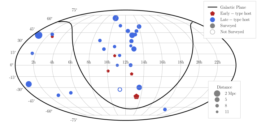
Figure 1: Position on the sky of the ELVES host sample. Hosts are colored by their morphology: late-type spirals vs. early-type ellipticals and lenticulars. Point size indicates the host distance. The unfilled point labelled ‘Not Surveyed’ indicates a host where we have no survey coverage (NGC 3621). All other hosts have candidate satellite lists.

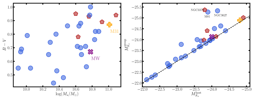
Figure 2: Properties of the full ELVES host sample. Left: The host color vs. stellar mass. Points are the same as in Figure 1. Right: Host $K_{s}$ luminosity vs. group $K_{s}$ luminosity. The three hosts with the largest difference between the two luminosities are labelled. NGC 3379 and NGC 3627 are the primaries of the Leo I and Leo Triplet groups, respectively.

The on-sky locations of these hosts are shown in Figure 1. In Figure 2, we show various properties of the host sample. The hosts are fairly evenly distributed between $10^{10}$ and $10^{11}$M${}_{\odot}$  in stellar mass. The right panel shows the group $K_{s}$ luminosity (the sum of the luminosity for all group members) reported in the group catalog of kourkchi2017 versus the luminosity of just the primary host. In most cases, these values are quite close, indicating the host completely dominates the luminosity of the group. For a few cases, the group luminosity is significantly larger than that of the primary host. These include the M81/M82 group, the Leo I group, and the Leo Triplet (labelled in the Figure), each of which has several massive galaxies. In previous papers on this survey, we have referred to these hosts as ‘small-groups’ to distinguish that they are notably higher mass than bona fide MW-analogs.

3 Observational Data

The full ELVES survey is an extension of our earlier survey presented in carlsten2020a; carlsten2020b. That work presented a set of LV hosts surveyed with archival CFHT/MegaCam data. The ELVES sample is considerably expanded by using the extremely wide-field DECaLS imaging data sets (decals; bass1; bass2).

As stated above, the process of cataloging nearby satellite systems is two-fold. First, candidate satellites need to be detected either visually or with an automated algorithm. Second, the candidate satellites need to have their distances measured to confirm that they are actually physically associated with a purported host. In carlsten2020a; carlsten2020b, the CFHT/MegaCam data was of high-enough quality to do both steps, with the second step being accomplished via measurements of surface brightness fluctuations (SBF). However, the DECaLS data is almost always too shallow and with too poor of seeing to do the distance measurements, and thus we generally only use it for the object detection. The distance measurements come from SBF using various follow-up data, including archival Hyper Suprime-Cam (HSC) and new Gemini and Magellan imaging.

Table 1 lists the data sources used for each host, including for candidate detection and distance confirmation. The table also lists data sources for the satellite photometry used throughout the paper, which is almost always the same as the candidate detection data, except for where we use a literature reference for the satellite detection. Overall, we use literature sources for the satellite lists for 5 hosts (MW, M31, CenA, NGC 5236, and M81) and do our own object detection for 25 hosts. 17 of these use DECaLS imaging, 6 (NGC 1023, NGC 4258, NGC 4565, NGC 4631, NGC 5194, and M104) use the CFHT/MegaCam search of carlsten2020a, one (NGC 891) uses separate CFHT/MegaCam data, and one (NGC 6744) uses (non-DECaLS) DECam data.

Regardless of the source for the imaging data, we always use two bands for candidate detection: either $g/r$ or $g/i$. The one exception is NGC 891, where for about half of the surveyed area, only $r$-band data are available. Deeper follow-up data for distance confirmation are often only a single band (either $r$ or $i$) since those are the ideal SBF bands, and a color measurement already exists from the candidate detection data.

The reduced DECaLS imaging data are taken directly from the web server where $g$ and $r$ band data are available for download. We use DECaLS DR8 for the candidate detection but have redone the satellite photometry using DR9 as the DR9 reduction includes a more optimized sky-subtraction for LSB galaxies. Overall, we find minimal difference between DR8 and DR9.

CFHT/MegaCam data are downloaded raw from the CFHT archive server and are reduced in the fashion described in sbf_calib and carlsten2020a. DECam data that are not part of DECaLS (NGC 6744 is the only host that uses this) are downloaded raw from the NOIRLab archive and reduced in a very similar way to the CFHT data. Generally, SDSS (sdss_df14) or Pan-STARRS (panstarrs; panstarrs2) are used for the photometric calibration. For the few southern hemisphere hosts outside those footprints, we use Gaia (gaia_dr2) or APASS (apass) for the photometric calibration.

Gemini/GMOS data are reduced using the DRAGONS software package. Gemini/GMOS data from programs FT-2020A-060, US-2020B-037, and US-2021B-0018 (PI: S. Carlsten) are used. Magellan/IMACS data are reduced using a custom pipeline that does all the main steps in a similar way to the MegaCam and DECam pipelines. Finally, the HSC data are downloaded from the Subaru archive and reduced using the pipeline written by the HSC team (bosch2018). All HSC data are archival and include (but are not limited to) data from the HSC-SSP survey (aihara2018; aihara2019).

All of these telescopes and camera systems use Sloan-like filters. However, there will be some slight differences between the different filter sets. Following carlsten2021a, we do not make any attempt to bring them all onto the same filter system. That work (Figure 16 in that paper) showed that the differences between the filters is expected to be $\lesssim 0.1$ mag based on synthetic photometry from stellar evolution models (mist_models). One instance where systematic offsets of this magnitude might matter is integrated color. However, the effect of this systematic uncertainty in inferring stellar mass (the primary use of color) is generally less than the statistical uncertainty coming from photon noise and/or sky subtraction issues and thus we do not account for it.

The actual areal coverage of each host is shown in Appendix LABEL:app:host_areas. For the DECaLS hosts, we almost always are able to extend fully to 300 kpc, an approximate value for the virial radius of halos of the typical mass expected for most ELVES hosts ($M_{\mathrm{halo}}\sim 10^{12}$M${}_{\odot}$). We note that the halo masses of the most massive hosts in the ELVES sample (e.g. M104, NGC 3627, and NGC 3379) are likely closer to $\sim 10^{13}$ (karachentsev2014_masses; kourkchi2017) and will have much larger virial radii. On the other hand, the least massive ELVES hosts (e.g. NGC 3344 and NGC 4517) will have smaller virial radii. The hosts from the non-DECaLS data sources (CFHT/MegaCam or DECam) all have less coverage. For a couple of these (NGC 4631 and NGC 4258), we extend the CFHT/MegaCam data with some DECaLS data and additional SBF follow-up, with the specific footprints shown in Appendix LABEL:app:host_areas. The approximate radial extent of the search footprints for each host are listed as $r_{\mathrm{cover}}$ in Table 1.

4 Candidate Satellite Detection

For the 25 hosts where we conduct our own candidate satellite detection, we apply the semi-automated detection algorithm optimized for LSB dwarf galaxies detailed in carlsten2020a. This algorithm draws heavily on the LSB galaxy detection pipelines of bennet2017 and greco2018.

We use a custom search algorithm as opposed to simply using common object detection algorithms (e.g. SExtractor, sextractor), because those algorithms are not optimized for large, diffuse, LSB dwarf galaxies. Such sources are likely to get “shredded” (i.e. over-deblended). More advanced algorithms (e.g. noise_chisel; lang2016; profound; melchior2018; haigh2021) are being developed that demonstrate promise for LSB dwarf surveys (venhola2021). While our search algorithm is more complicated than simply using SExtractor, it still does make use of SExtractor in multiple ‘hot-and-cold’ runs (i.e. runs with high and low thresholds, see below) intermixed with aggressive masking.

Like many other object detection algorithms, the one used here explicitly separates source detection from source extraction. In this section, we detail the first step which is simply to find the dwarf galaxies. A later section (§6) describes how we measure the photometric properties of the candidate satellites.

4.1 Overview of Detection Algorithm

The search algorithm is detailed in carlsten2020a and is applied essentially unchanged to the DECaLS data, but we provide a brief overview of the important steps in this section. The main steps of the process are:

1. Create bright star masks from Gaia star catalogs for stars brighter than $20^{th}$ magnitude. Custom shaped masks that cover the scattered light halos and saturation spikes of bright stars are applied to all of the survey fields.

2. Initial detection step with a large size and moderate significance threshold to find large, relatively high surface brightness candidate satellites. In particular, SExtractor is run with a $5\sigma$ threshold and $\sim 2000$ pixel minimum area (corresponding to a radius of $\sim 7$${}^{\prime\prime}$  for a circular source). To remove some massive background galaxies, an effective surface brightness cut of $\langle\mu\rangle_{r_{e}}\gtrsim 22$ mag arcsec${}^{-2}$ (calculated from SExtractor fluxes and sizes) is applied to the detections. Note that this is not the only stage where relatively massive satellites can be detected as their diffuse/LSB outskirts will also be detected in the LSB detection step below (and dwarfs universally have diffuse outskirts, see kadofong2020).

3. Mask bright sources and their associated diffuse emission as in greco2018. Sources are detected with both a high, $15\sigma$, and low, $\sim 1\sigma$, detection threshold. The LSB detections are associated with a high surface brightness (HSB) detection if they overlap more than a certain fraction ($5\%$) of their pixels with the HSB detection. The detected LSB pixels that do get associated with an HSB detection get masked. These represent, for example, the extended envelopes of background galaxies, intracluster light from galaxy clusters, and/or scattered light around stars not bright enough to be covered by the Gaia star mask. After this step, there is a another simple masking of all sources over $\sim 4\sigma$ above the background.

4. Filter the image to emphasize diffuse, LSB emission. The masked image is convolved with a Gaussian with FWHM $\sim 2\times$ the field’s PSF size.

5. Second detection step with a low threshold to find faint candidate satellites. Sources in the masked and filtered image are detected with a significance threshold of $\sim 2\sigma$ and size greater than $\sim 800$ pixels (corresponding to a radius of $\sim 4$${}^{\prime\prime}$  for a circular source).

6. Visual inspection to remove artifacts and other false positives. The vast majority ($>95\%$) of the things removed in this step are clear artifacts such as saturation spikes or emission from bright stars or the outskirts of massive elliptical galaxies that leaked through the masks. Additionally, detected galaxies that are clear background contaminants are removed. For instance, small ($r_{e}\lesssim 5$${}^{\prime\prime}$) galaxies that have well-defined spiral arms or a bulge$+$disk morphology are clearly not in the Local Volume. Low-mass dwarfs will necessarily be fairly featureless and diffuse. carlsten2020a gives more details on this step and examples of visually rejected galaxies. Often during this step, particularly ambiguous detections are queried in Simbad and any galaxies with known redshifts more than $275$ km/s greater than the host are background objects and not further considered.

The first five steps are done independently in the $g$ and $r$ (or $i$) bands and then the two detection catalogs are merged before the visual inspection step. Objects need to be detected in both bands to pass to the visual inspection step.

Many of the algorithm’s parameters needed to be slightly tweaked for each field to account for the differing depths of the different datasets and host distances. Each parameter preceded by a $\sim$ in the description above was often tuned for each host. Hosts with shallower imaging, for instance, needed a larger smoothing kernel (i.e. more blurring), and more nearby hosts had larger size thresholds for detected objects. The parameters were tuned in an initial step where a subset of the survey coverage for each host was visually searched for candidate satellites against which the algorithm was tested. The specific parameters used for each host are not particularly important to the results as the search algorithm’s completeness for each host is quantified using those same parameters. Thus, all affects they have on the search completeness are accounted for.

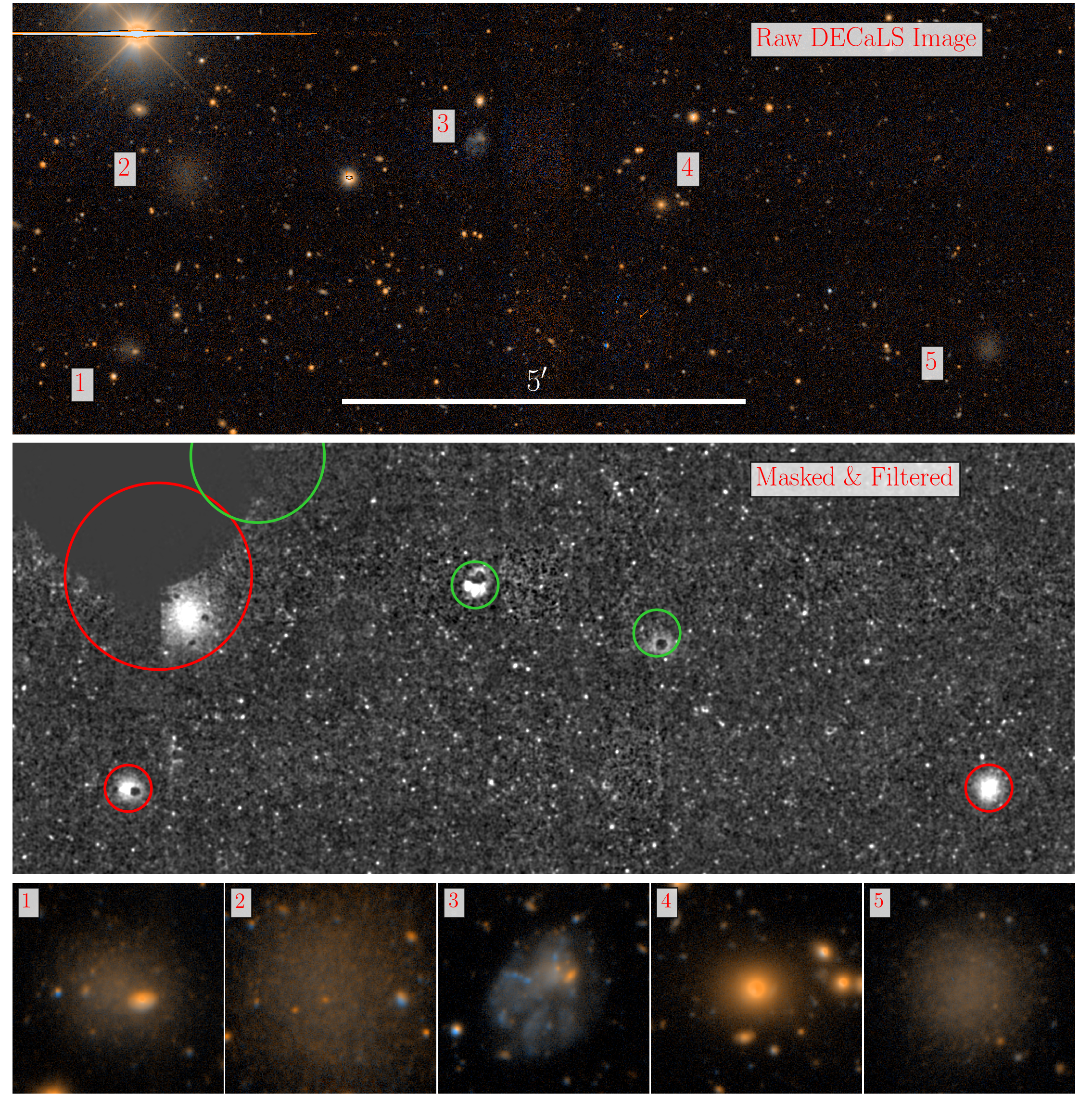
Figure 3: Demonstration of the detection algorithm on a surveyed area near NGC 3379. Top panel shows the raw DECaLS detection images ($g+r$ color composite). The middle panel shows the detection image after it has been masked for bright stars and galaxies and has been filtered to bring out LSB emission. Detections from the pipeline are shown as circles. The detections that pass visual inspection are in red while those that do not are shown in green. The rejected detection in the top left is from scattered light from the bright star leaking through the mask while the other two detections are clear background galaxies (see text for more details). The five labeled detections are shown in the bottom row in deep HSC images. These images are not used in the detection process but are used to confirm the candidate satellites via SBF distance measurements. The images on the bottom row are 40${}^{\prime\prime}$  (2 kpc at the distance of NGC 3379) to a side.

Figure 3 demonstrates the main steps through an example part of the field around NGC 3379, the main host of the rich Leo I group. The top panel shows the raw DECaLS image ($g+r$ color composite). The middle panel shows the image with bright stars and background galaxies masked and filtering applied. The masking in Step 3 above is clearly quite aggressive, but we show in the next section on completeness that it is not overly aggressive because it does not completely mask candidates. The detections from Step 5 are shown as the superimposed circles. Those that pass visual inspection are in red while those that are rejected are in green. The five detections that are labeled in the top image are shown in close-up in the bottom row using extremely deep ($>2$ hour integration) HSC images. The sixth rejected detection is simply emission that leaked around the star mask and is not shown in close-up. Detections 1, 2, and 5 are high-quality candidate satellites. In fact, these candidates are all confirmed satellites via SBF distance measurements. The two rejected detections (3 and 4) are background galaxies. Object 3 has a complicated morphology and small size ($r_{e}\sim 5$${}^{\prime\prime}$), indicating it is not in the Local Volume. In this case, its HI redshift from ALFALFA (haynes2018) of several thousand km/s greater than that of NGC 3379 confirms this, although not all visually rejected galaxies have redshifts. Object 4 is a massive background elliptical whose outskirts leaked through the masking. While this visual inspection step might appear to introduce ambiguity, visual selection of dwarfs in the Local Volume is a powerful tool due to their proximity (e.g. karachentseva1968; karachentsev2007) and many contemporary searches are primarily visual (e.g. byun2020; habas2020).

The median false positive rate as determined by the visual inspection step is $\sim 30$ rejected detections (e.g. artifacts, halos around bright stars, or background galaxies) for each candidate satellite. As stated above, this is mostly a result of insufficient masking of bright stars or bright background galaxies that allows too much emission to pass through. This step did require a fairly significant amount of human involvement, meaning that this algorithm is not scalable for the extremely wide-field surveys of the Roman Space Telescope or Vera Rubin Observatory. For the relatively small areas surveyed in ELVES ($\sim 400$ square degrees total), removing these contaminants by visual inspection was tractable.

4.2 Completeness of Surveys

In order to facilitate comparison to other satellite dwarf searches and theoretical models, it is critical to quantify the completeness of the survey. We do this by injecting artificial galaxies into the survey images and quantifying the fraction of injected galaxies recovered as a function of input luminosity and size. The fact that our search process is semi-automated (as opposed to purely visual) greatly facilitates this process. We do not apply any visual inspection step to the artificial galaxies and assume that any injected galaxy detected by the search algorithm would pass the visual inspection. In this section, we describe the artificial galaxy injection and show the overall average completeness of the survey.

The process for injecting artificial galaxies is detailed in carlsten2020a. The DECaLS and non-DECaLS hosts are treated a little differently, primarily in that the non-DECaLS hosts have their artificial galaxies injected at the chip level before sky subtraction and coaddition. On the other hand, the DECaLS hosts have their artificial galaxies injected directly in the coadds due to the significantly larger volume of imaging data, both in number of hosts and area covered per host. In either case, exponential profiles (i.e. $n=1$ Sérsic profiles) are injected at various $r$ or $i$ luminosities and central surface brightness levels, with colors in the range $g-r\in[0.3,0.6]$ or $g-i\in[0.4,0.8]$ depending on which filters are used. The data are then run through the detection pipeline, and the fraction of galaxies in each luminosity and surface brightness bin that are recovered is recorded. Simulated dwarfs that fall on top of areas lost to the star-masking are not treated differently, thus, we do not expect the recovery fraction to ever be $100\%$. The area lost to star-masking is generally around $\sim 5\%$.

As shown in carlsten2021a, the input galaxy parameters roughly resemble the Sérsic indices and colors of the real satellites, both quenched and star-forming. However, true dwarf galaxies generally have slightly lower average Sérsic index of $n\sim 0.7$, a result also seen in other surveys (e.g. eigenthaler2018; ferrarese2020). At fixed luminosity and central surface brightness, a higher Sérsic index dwarf will be more difficult to find since more of the emission will be be at a very low surface brightness level in its outskirts, and more likely to be buried in the sky noise. Thus, we expect these completeness estimates to be slightly conservative.

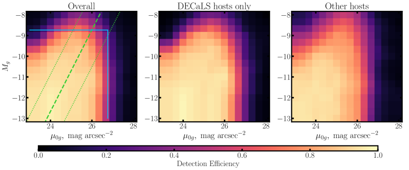
Figure 4: Average completeness of the dwarf searches as quantified by image simulations with injected artificial galaxies. Left panel shows the average of all hosts, while center and right panels split the hosts by the source of the imaging data. The blue region in the left panel demarcates the completeness quoted in prior ELVES papers ($M_{V}<-9$ mag and $\mu_{0,V}<26.5$ mag arcsec${}^{-2}$). The green dashed line shows the mass-size relation of carlsten2021a converted into this plane, and the green dotted lines show the $1\sigma$ intrinsic scatter measured in the mass-size relation.

Figure 4 shows the results of the injection simulations. The left panel shows the average recovery fraction across all 25 hosts. In doing the average, the hosts are weighted by the number of confirmed and possible satellites (see §5 below). The center and right panels show the average recovery fraction of the DECaLS hosts separately from the other hosts (primarily CFHT/MegaCam hosts).

Results for individual hosts are shown in Appendix LABEL:app:host_completeness. The recovery fractions are generally similar across the different hosts and data sources. We note that the BASS part of DECaLS (which 4 DECaLS hosts use) and the CFHT/Megacam data used for NGC 891 are significantly shallower than the rest of the hosts with the surface brightness completeness being $\sim 0.5$ mag lower. However, this is a relatively small number of hosts, and we do not further distinguish these from the others.

The blue region in the left panel of Figure 4 shows the completeness limits quoted in previous ELVES papers: $M_{V}<-9$ mag and $\mu_{0,V}<26.5$ mag arcsec${}^{-2}$, assuming $g-V\approx 0.25$ mag. The green dashed line shows the mass-size relation of carlsten2021a converted into this plane assuming $M_{\star}/L_{g}=1.24$ which comes from the color-$M/L$ relation of into2013 and the average color of $g-i=0.74$. An $n=1$ Sérsic profile is assumed in determining the central surface brightness from luminosity and effective radius.

Overall, the recovery fraction is $\sim 90-95\%$ at bright magnitudes and surface brightness, reflecting the area lost from the search to star masks. There is a clear drop-off in completeness between $\mu_{0,g}\sim 26-27$ mag arcsec${}^{-2}$. The $\mu_{0,V}<26.5$ mag arcsec${}^{-2}$ we have quoted in the past is roughly the 50% completeness limit.

In addition to the artificial galaxy injection tests, our completeness is proven through comparison with previous satellite searches in the literature for several of the ELVES hosts. In Appendix LABEL:app:prev_work, we go through the hosts in more detail, and provide detailed comparison with previous searches from the literature for hosts that have them. The comparisons are quite favorable for ELVES with no candidate satellites missed above the asserted completeness level across the 8 ELVES hosts that have been significantly surveyed in the past.

For the five hosts that we do not perform our own object detection (MW, M31, CenA, M81, M83), we assume they are complete down to the fiducial level of $M_{V}<-9$ mag and $\mu_{0,V}<26.5$ mag arcsec${}^{-2}$. The actual completeness limits of these literature surveys are generally quite a bit deeper due to the closer proximity of these hosts relative to most ELVES hosts. Details can be found in the sources for those satellite lists (see Table 1).

While we do detect numerous candidate satellites fainter than $M_{V}=-9$ mag, all ELVES satellite lists and figures in this paper have a $M_{V}<-9$ mag cut applied to them.

5 Candidate Satellite Confirmation

In this section, we describe the process of confirming candidate satellites as actual physical satellites of a LV host. Many of the candidate satellites have prior distance information, either HST-based TRGB distances or redshift, but the majority do not. Thus, we rely heavily on efficient surface brightness fluctuation (SBF) measurements to provide a large number of distance constraints with modest ground-based data. We try to constrain the distance to as many candidate satellites as possible, but several remain with no distance constraints. We keep careful track of these ‘unconfirmed/candidate’ satellites throughout this paper as they require special treatment in any analysis using ELVES satellite lists.

5.1 SBF Measurement

Details of the SBF measurement are given elsewhere (sbf_calib; carlsten2020b), so we only provide a brief summary here. SBF entails measuring how ‘patchy’ a galaxy is in the semi-resolved regime. Distance smooths out Poisson fluctuations in the number of bright stars per resolution element such that a galaxy will look smoother further away. In measuring a galaxy’s SBF, this ‘patchiness’ is quantified as the ‘SBF magnitude’, $\bar{M}$.

To quantify this, we start with a smooth model of the galaxy’s surface brightness profile. The reddest band we have ($r$ or $i$) is modeled, as SBF is brighter and seeing is generally better for redder pass-bands (e.g jensen2003; scott_psf). Due to the small sizes and low luminosities of most of the dwarfs, we always use a parametric Sérsic profile as a model for the smooth profile (see §6 for more information on the Sérsic profile photometry). This model is subtracted out from the raw image and the result is normalized by dividing it by the square root of this model. We then calculate the azimuthally averaged power spectrum of this result via a fast Fourier transform. The fluctuation power due to SBF is the component of the power spectrum on the scale of the PSF. For details on how we mask contaminants, we refer the reader to (sbf_calib; carlsten2020b).

5.2 SBF Calibration

Due to the fact that the average brightness of stars in a galaxy will depend on the stellar population, the level of SBF also will depend on the stellar population present in a galaxy. Thus a calibration is used to relate the absolute SBF magnitude to galaxy color. For $i$-band measurements, we use the calibration provided in sbf_calib, while for $r$-band measurements, we use the calibration in carlsten2020b.

These calibrations are specifically for CFHT/MegaCam. In this work we use five different telescope and instrument combinations (CFHT/MegaCam, Subaru/HSC, Blanco/DECam, Gemini/GMOS, and Magellan/IMACS) that all have Sloan-like $r/i$ filters and that all will be slightly different. However, from experiments calculating theoretical SBF magnitudes using the MIST isochrones and synthetic photometry (mist_models) for MegaCam, HSC, and DECam, we find that the SBF magnitudes are always the same within $\sim 0.1$ mag, which is small compared to the statistical error of the SBF measurement. With that said, we do incorporate a small $-0.1$ mag adjustment to the CFHT-based calibration when using DECam filters. We do not perform any adjustments when using HSC, GMOS, or IMACS data, however. kim2021 show that their empirical SBF calibration in the HSC filter system is quite close to that of sbf_calib with any difference more likely attributable to different masking strategies than filter differences.

5.3 SBF Distances

With the SBF measurements and calibration in hand, we can constrain the distance to each dwarf. Following carlsten2020b, there are three outcomes to this measurement. First, if the SBF measurement is of high S/N ($>5$) with a distance that is consistent with that of the host within $2\sigma$, we consider the candidate satellite to be a ‘confirmed’ satellite. Second, if the $2\sigma$ lower bound of the SBF distance constraint is beyond the distance of the host, we consider the candidate to be rejected as a background contaminant. The actual distances of these objects are generally not known as the SBF measurement only sets a distance lower bound from the absence of measurable SBF. Third, if the SBF measurement is of too low S/N and the distance lower bound is within the distance of the host, the candidate is kept in the ‘unconfirmed/candidate’ satellite category. These objects may or may not be satellites and need deeper data or HST observations for their satellite status to be decided.

We use this cutoff of S/N $>5$ in the SBF measurement as a safeguard against false positive satellite confirmation. In our experience, this S/N level is roughly where SBF becomes clearly distinguishable from other sources of fluctuation power, such as scattered star-forming clumps in the galaxy or background galaxies. sbf_m101 used SBF to confirm two satellites around NGC 5457 (M101). These satellites had SBF S/N $\gtrsim 7$, above the threshold used here. Both of these have since been confirmed by HST TRGB distances in bennet2019. sbf_m101 also discussed 2 other candidates as promising follow-up targets that had moderate signal with S/N$\sim 2-3$. The HST imaging of bennet2019 showed that the galaxies were background contaminants. The small fluctuation signal appeared to be coming from unmasked background galaxies, not SBF. Using the threshold adopted here, these two candidates would be conservatively included in the ‘unconfirmed/candidate’ satellite category.

In sbf_calib, we showed that the ground-based SBF distances agreed with HST TRGB distances with an RMS of $15\%$. While this is lower precision than the $\sim 5-10\%$ precision that HST TRGB distances can attain (beaton2018), it is still quite useful in confirming or rejecting candidate satellites as actual, physical satellites of a certain host. Thus, by including satellites with SBF distances within $2\sigma$ of the host, we do expect that some near-field dwarfs (e.g. dwarfs analogous to the Local Group field dwarfs nearby to the MW) will be included as ‘satellites’. Experimenting with halos from the IllustrisTNG simulations (tng1; tng2), in carlsten2020b, we found that this distance constraint led to a contamination of field interlopers of around $15-20\%$. Until more precise distances are possible, nothing can be done regarding this contamination, and it must be kept in mind when analyzing ELVES satellite lists. We note that this is a similar contamination fraction to what occurs when selecting satellites with a recessional velocity cut, as in the SAGA Survey (mao2020).

5.4 Other Distance Information

In addition to SBF measurements, we make use of TRGB distances and redshift information, when available. We search the Updated Nearby Galaxy Catalog of karachentsev2004; karachentsev2013 for TRGB distances for all of the candidate satellites. Similarly, we query SIMBAD for any redshift information. Dwarfs with TRGB distances within $1\sigma$ (or 1 Mpc, if no distance uncertainty is available) of the distance to their host are considered ‘confirmed’ with those outside of this range rejected as contaminants. For dwarfs with redshifts, those with velocities within 275 km/s of their host are confirmed satellites (e.g. mao2020) while those outside this range are rejected. We note that the search for redshift information often occurs very early on in the candidate detection pipeline (in particular, in the visual inspection step) with background contaminants being removed at this point, even before the candidate satellite stage. Thus, many otherwise passable candidate satellites are not in the final candidate satellite lists since they had redshift information indicating they are background.

Table 2: Overview of Distance Constraints.

Name	$M_{K_{s}}^{\mathrm{group}}$	# candidates	# SBF conf.	# other conf.	# SBF rejected	# other rejected	# unconfirmed
	(mag)
NGC253	-23.96	8	0	5	0	2	1
NGC628	-22.81	17	7	6	3	0	1
NGC891	-23.83	8	1	2	1	0	4
NGC1023	-23.98	22	9	5	5	0	3
NGC1291	-23.97	21	12	2	1	2	4
NGC1808	-23.78	18	7	3	4	0	4
NGC2683	-23.50	12	3	3	2	0	4
NGC2903	-23.69	16	4	3	9	0	0
NGC3115	-24.14	27	13	4	8	0	2
NGC3344	-22.27	9	3	0	2	0	4
NGC3379	-25.37	85	16	28	17	2	22
NGC3521	-24.41	18	9	2	6	0	1
NGC3556	-22.76	17	0	1	2	1	13
NGC3627	-25.33	33	6	14	1	0	12
NGC4258	-23.94	21	3	4	12	1	1
NGC4517	-22.16	56	7	2	39	8	0
NGC4565	-24.27	11	2	2	2	0	5
M104	-25.01	18	11	0	3	0	4
NGC4631	-22.90	23	7	5	8	2	1
NGC4736	-23.10	17	0	7	0	3	7
NGC4826	-23.24	12	3	4	2	1	2
NGC5055	-24.04	13	5	4	0	0	4
NGC5194	-24.51	13	2	1	8	2	0
NGC5457	-23.16	42	2	7	33	0	0
NGC6744	-24.00	15	4	1	4	0	6
M31	-24.89	–	–	20	–	–	–
M81	-25.27	–	–	24	–	–	–
CENA	-24.41	–	–	22	–	–	–
NGC5236	-23.67	–	–	11	–	–	–
MW	-24.13	–	–	10	–	–	–
Total	–	552	136	202	172	24	105

Note. — Overview of the distance confirmation results. For each host the total number of candidates, number of confirmed satellites, number of rejected background contaminants, and number of remaining unconfirmed/possible satellites are given. The numbers of confirmed and rejected dwarfs are split by whether the constraint is from SBF or otherwise (TRGB and/or velocity). Many of the satellites confirmed via redshift or TRGB also have an SBF distance with overall close agreement between the methods. The five previously surveyed hosts are given at the bottom with the bottom-most row listing the totals in each category.

5.5 Distance Results

The distance results for all the satellites for which we found or measured a distance are provided in Appendix LABEL:app:distances. There are three tables: one for dwarfs which get confirmed as satellites, one for dwarfs that get rejected as contaminants, and one for dwarfs that remain as possible/candidate satellites. We do not provide any distance constraints for these latter dwarfs since any distance constraints for them are, by definition, not informative. However, we do list what data source was used, if any, in attempting an SBF distance.

Table 2 gives an overview of the distance results, including number of confirmed and rejected objects and number of lingering unconfirmed/possible candidates that did not have conclusive distance results. All together, including the five previously surveyed satellite systems (MW, M31, M81, CenA, NGC 5236), there are 338 confirmed satellites and 105 remaining candidates. 136 of these confirmed satellites are confirmed via SBF measurements. Only 31 ($23\%$) of these SBF-based confirmations came from our previous work in carlsten2020b. In total, there are 182 confirmed satellites with SBF distances, with 53 also having other distance confirmation (either TRGB or redshift). In all but four cases ($7.5\%$), the SBF result agrees with the TRGB or redshift result. In these few exceptions, there is some issue (e.g. nearby bright star halo or irregular morphology) that clearly biases the SBF measurement, causing it to be inaccurate. These are discussed more in Appendix LABEL:app:distances.

5.6 Candidate Satellite Contamination Estimate

In this section, we provide a simple estimate for the probability that each of the remaining unconfirmed/possible candidates is a real satellite of its host. To do this, we consider the fraction of similar candidate satellites that did have conclusive distance results (either from SBF or otherwise) that ended up being confirmed as a satellite.

We do this as a function of luminosity and surface brightness as the likelihood a candidate is an actual satellite will depend on these. This is similar in principle to the $\mathcal{R}_{\mathrm{sat}}$ estimate in the SAGA Survey (see §5.3 of mao2020) that accounts for photometric candidates in that work that did not have robust spectroscopic measurements.

Figure 5 shows the surface brightness versus luminosity relation for candidates that had conclusive distance constraints (either confirmed as a satellite or rejected). The luminosity of a background contaminant is calculated as if it was at the distance of the host. In most cases, the actual distance of these contaminants are not known; the SBF results only show that they must be beyond the distance of the host. The confirmed satellites show a clear relation between surface brightness and luminosity (this is explored in more detail in carlsten2021a) whereas the rejected contaminants are generally higher surface brightness with smaller sizes. This is suggestive that most of the background contaminants are dwarf galaxies that are $\sim 2-3\times$ further in distance than the LV hosts. The confirmed and rejected dwarfs are clearly segregated in the $M_{V}-\mu_{0,V}$ plane such that the location of an unconfirmed/possible candidate in this plane contains information on how likely it is to be a real satellite.

To quantify the likelihood of each unconfirmed/possible candidate being real, we simply consider the 20 nearest candidates that had conclusive distance results in the $M_{V}-\mu_{0,V}$ plane and calculate the fraction of those that were real satellites. We find very similar results if we had instead used anywhere between the 10 to 50 nearest candidates. The right panel of Figure 5 shows the value of the confirmed fraction at different locations in the $M_{V}-\mu_{0,V}$ plane.

There are several simplifying assumptions being made in constructing this likelihood estimate. The first is that this estimate will certainly not take into account the host-to-host scatter in the contamination fraction due to prominent background groups along the line of sight. For instance, NGC 5457 and NGC 4517 have significant contamination due to rich background groups at $D\sim 15-30$ Mpc.

Second, it implicitly assumes that the threshold in data quality required to confirm a satellite via SBF at a given luminosity and surface brightness is the same as that required to reject a background contaminant at that luminosity and surface brightness. It is easy to understand why this assumption is important if we consider an alternate scenario where, for instance, rejecting a background contaminant is possible with much worse data than that required to confirm a satellite (for instance if we required a S/N $>100$ measurement of the SBF to ‘confirm’ a dwarf). In this case, the rejected contaminants would be over-represented in the set of candidates with conclusive distance results, and Figure 5 would underestimate the likelihood that an unconfirmed candidate is a real satellite. We test this assumption in Appendix LABEL:app:sbf_sims where we show the results of applying the SBF confirmation and rejection criteria (see §5.3) to simulated dwarf galaxies across a range in luminosity and surface brightness. Taking two different hosts (NGC 4258 and NGC 3379) with high-resolution, deep data as examples, we simulate both dwarfs with SBF at the level appropriate for the distance of the host and dwarfs without SBF, representing background contaminants. Given a level of data quality, it is possible to reject candidates that are fainter by about a magnitude (in luminosity or surface brightness) than the faintest candidates that can be confirmed with that data. This discrepancy would be decreased if we did not require a S/N $>5$ measurement of the SBF to consider a dwarf ‘confirmed’, but we explained the rationale behind that criterion in §5.3. This $\sim 1$ mag difference is smaller than the dynamic range of the remaining candidates, and we expect this estimate of the confirmed fraction is fairly accurate. With that said, we recommend any analysis that uses ELVES satellite lists to test their results considering the cases where all or none of the remaining candidates are real satellites.

In total, summing these satellite probability estimates for all 105 remaining unconfirmed objects yields 49.8 real satellites, meaning that, most likely, there are an additional $\sim 50$ actual satellites amongst the unconfirmed candidates. The SAGA Survey (§5.3 of mao2020) estimates a total of 24 actual satellites amongst the candidates that did not have successful spectroscopic follow-up. As a fraction of the total number of confirmed satellites in each survey, this is a similar rate of failure in distance follow-up between the two surveys.

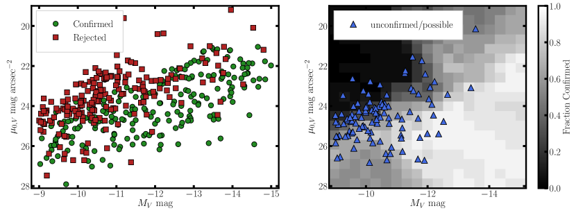
Figure 5: A simple estimate for the probability that the remaining unconfirmed/possible candidates are actual physical satellites. The left panel shows the luminosity and surface brightness of both the confirmed satellites and the rejected contaminants (if the latter were to be at the distance of their purported host) that had conclusive distance constraints. The confirmed satellites show a pronounced luminosity-surface brightness relation while background contaminants tend to be smaller with higher surface brightness. The right panel shows an estimate for the likelihood that a candidate will turn out to be a real satellite as a function of luminosity and surface brightness. This likelihood is estimated from the fraction of confirmed satellites out of the closest 20 confirmed or rejected candidates for each point on the $M_{V}$-$\mu_{0,V}$ plane. The locations of the actual remaining candidates are over-plotted.

6 Properties of the Satellites

In this section, we turn to how we measure various properties of the satellites, including optical and UV photometry.

All satellite photometry is in the AB system and corrected for MW dust extinction using the $E(B-V)$ maps of sfd recalibrated by sfd2. We take the solar $g$-band magnitude to be $M^{\odot}_{g}=5.03$ mag (willmer2018).

6.1 Optical Sérsic Photometry

The primary photometric results come from fitting the optical images with Sérsic profiles. We refer the reader to carlsten2021a for an in depth description of how the Sérsic profiles are fit to the galaxies. In brief, the $g$-band images are fit first since they are generally deeper, and then the $r$- or $i$-band image is fit using the shape parameters fixed, varying only the intensity. The masking threshold and image cutout size are adjusted in an iterative fashion to minimize the dependence that the final photometry results have on those choices.

As detailed in Table 1, the photometry always uses DECaLS/DECam or CFHT data. Even though we have deeper Gemini, Magellan, and Subaru data for many dwarfs for SBF, we do not present the photometry from that data in an attempt to limit the number of filter systems used. For three of the five previously surveyed systems (M81, CenA, and NGC 5236), we are able to provide photometry using our consistent methodology for almost all of the satellites. There were a few M81 satellites out of the DECaLS footprint and a few CenA satellites not covered in DECam archival data.

Following carlsten2021a, we estimate uncertainties in the photometric parameters from image simulations where we inject Sérsic profile galaxies into CFHT or DECaLS data and quantify how well the input values are recovered. carlsten2021a also gives the equations we use to convert between $g-r$ and $g-i$ and convert $g$-band photometry into $V$-band.

For each dwarf, we use the color and $g$-band luminosity to estimate its stellar mass using the color-mass-to-light ratio relations in into2013. For several of the brightest ($M_{V}\lesssim-18$ mag) satellites, we did not attempt Sérsic photometry due to the clear inadequacy of a single profile in fitting these large, complicated galaxies. Instead, for these we simply provide stellar mass estimates calculated from 2MASS (2mass) $M_{K_{s}}$ values from kourkchi2017. For the MW and M31 satellites, we do not have colors but use average color-luminosity trends from the dwarfs that do to separately define luminosity-mass to light ratio relations for early- and late-type dwarfs (see Equation 4 of carlsten2021a).

Appendix LABEL:app:sat_lists presents the main table for the photometry of the satellites. The confirmed and possible satellites are all given in one table, along with a flag to indicate which satellites have robust distance confirmation.

6.2 Galaxy Morphology

In addition to the optical photometric measurements, we visually classify each dwarf to have either late- or early-type morphology. We use all available optical imaging, including the deep data often available for SBF measurements, to make this distinction. Dwarfs with smooth, regular, and generally low surface brightness morphology are classed as early-types. On the other hand, dwarfs with clear star-forming regions, blue clumps, dust-lanes, or any other complications in their surface brightness profile are classed as late-type. Given the data available, we believe this is the most robust way to split the dwarfs. More details of this separation and color images of example dwarfs classified as early- and late-type can be found in carlsten2021a.

6.3 GALEX Data

To complement the optical photometry, particularly to provide more information on recent star formation, we use archival GALEX (galex) data to measure the UV photometry of the dwarfs, where available. We largely follow the methods of greco2018_two and karunakaran2021. For each confirmed dwarf, we search the MAST archive for GALEX coverage. We find at least some coverage in NUV and FUV for a majority of the confirmed dwarfs, 271 in total. About a third of these are only covered by the shallow GALEX All-sky Imaging Survey with the remainder having deeper data, often from the Nearby Galaxy Survey (galex2007) or the 11 Mpc H$\alpha$ and Ultraviolet Galaxy Survey (11HUGS; kennicutt2008; lee2011) both of which targeted many LV galaxies.

From the MAST archive, we download two files for each GALEX frame and filter: the intensity maps (-int.fits files; $I$) and the high resolution relative response maps (-rrhr.fits files; $R$). We use these frames to construct the variance image as: $V=I/R$.

Due to the fact that many of the dwarfs are not actually detected in the UV, we do not do Sérsic photometry like with the optical data. Instead, we perform aperture photometry using elliptical apertures with radii of twice the effective radii found from the optical Sérsic fits. Contaminating point sources are masked before performing the photometry with an initial sextractor (sextractor) run. The sky contribution to the flux is estimated from the median of 50 apertures placed in the vicinity of the galaxy.

The measured flux and uncertainty for the apertures are:

$$F =\sum_{i}I_{i},$$ (2)

$$\sigma^{2}_{F} =\sum_{i}V_{i}+\sigma_{\rm sky}^{2}/N,$$

with $i$ ranging over the pixels covered by the aperture and $\sigma_{\rm sky}$ being the standard deviation of sky values measured in the $N$ sky apertures. We use the zeropoints given in morrissey2007 to convert the measured fluxes to AB magnitudes and correct for galactic extinction using $R_{\rm NUV}=8.2$ and $R_{\rm FUV}=8.24$ (wyder2007).

We do not attempt to correct for emission outside of the $2r_{e}$ aperture. Even without this, we find good agreement when applying this methodology to the SAGA satellites (mao2020) compared to the GALEX measurements of karunakaran2021 who performed a curve-of-growth analysis. The aperture NUV magnitudes are biased high by $\lesssim 0.1$ mag. We also find good agreement with the FUV fluxes in the UNGC (karachentsev2013) for ELVES satellites that are in that catalog.

Appendix LABEL:app:sat_lists presents a table with the UV photometry for the confirmed satellites that have it. For dwarfs that had a S/N$<2$ result, we report $2\sigma$ upper limits to the UV flux.

7 Properties of the Satellite Systems

In this section, we briefly explore features and trends amongst the satellite systems, including the luminosity functions and abundance, spatial distribution, and star formation properties. In-depth comparisons with galaxy formation models are out of the scope of this survey overview paper but will be pursued in future papers.

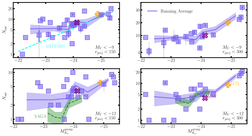
Figure 6: The satellite abundance versus the $K$-band luminosity of the host. Top row shows all satellites $M_{V}<-9$ mag, while the bottom row is restricted to the bright, $M_{V}<-12$ mag, satellites. The left panels show all hosts, but are restricted to satellites within $r_{\mathrm{proj}}<150$ kpc. Right panels show the subsample of hosts that are complete out to 300 kpc. Solid errorbars show the uncertainty in satellite abundance due to the unconfirmed satellites, using the satellite probabilities from §5.6. Dotted errorbars show the upper and lower limits of abundance if all, or none, of the unconfirmed candidates are actual satellites. The MW and M31 are plotted individually in the crosses. The solid lines show running averages. The abundance-$M_{K}$ relation from the ARTEMIS simulations (font2021) is shown in the upper left. The average trends from the SAGA Survey (mao2020) are shown in the bottom panels.

7.1 Satellite Abundance

The question of satellite abundance around MW-like galaxies has been a central component of the debate around ‘small-scale problems in $\Lambda$CDM’ for decades (e.g. moore1999; klypin1999; bullock2017). The abundance and luminosity function of satellites are sensitive probes to the underlying stellar-to-halo-mass relation (SHMR; e.g. gk_2017; nadler2020). Satellite abundance is also an important probe of recent accretion events experienced by a host (smercina2021). Using early results from ELVES, in carlsten2020b, we showed that the MW’s abundance of satellites was quite typical compared to LV systems of similar mass. We also showed that this abundance and the host-to-host scatter in satellite abundance were well-reproduced by recent galaxy formation models. In this section, we briefly highlight some abundance-related results and provide a comparison with recent SAGA Survey results (mao2020).

Figure 6 shows the relation between satellite abundance and host mass, as proxied by the group $K$-band luminosity. The group $K$-band luminosity is used instead of just the host’s in order to account for the groups with multiple massive primaries, like M81, NGC3627, and NGC3379. The top panels show all satellites down to the ELVES limit of $M_{V}<-9$ mag while the bottom panels show just the bright satellites, $M_{V}<-12$ mag. The left panels show the inner satellite systems, $r_{\mathrm{proj}}<150$ kpc, while the right panels show abundances out to $300$ kpc for the systems that are surveyed out that far. Running averages are shown in the blue bands. The unconfirmed satellites are included in the satellite counts using their satellite probability from §5.6 (Figure 5). The solid errorbars show the $1\sigma$ spread in abundance when stochastically including, or not, the unconfirmed candidates over many trials. The dotted errorbars show the upper and lower limits of abundance in the cases where all, or none, of the unconfirmed candidates turn out to be physical satellites. The lower panels show few errorbars because there are few unconfirmed candidates more luminous than $M_{V}=-12$ mag.

In all panels, a strong trend is seen between satellite abundance and host mass, as expected. Both the MW and M31 seem quite typical in terms of satellite abundance amongst similar mass systems. We found this result in carlsten2020b and show it here with a much larger statistical sample of hosts and satellites. This result is one of the primary results, if not the main result, from the ELVES survey.

In the top left panel, we show the scaling relation fit from the ARTEMIS simulation suite in font2021. This particular fit was using the ‘LV-selection’ which was chosen to mimic roughly the ELVES luminosity and surface brightness sensitivity (and restricted to the inner $r_{\mathrm{proj}}<150$ kpc regions). The fit reproduces the average abundance well, particularly at high host mass, but seems to underpredict the satellite abundance somewhat at the lowest masses. In fact, in all panels, the observed satellite abundance seems to flatten out at the lowest masses. Note that several of these low-mass hosts have complete, or nearly complete, distance confirmation for all candidates so this is not simply a floor caused by background contaminants. Including satellite abundances for even lower-mass, LMC-like, hosts will be an important extension of this work (see madcash; carlin2021; muller2020_low_mass, for initial work in this direction).

In the bottom panels we show a comparison to the average trends from the SAGA Survey (mao2020). The $M_{V}<-12$ mag cut used closely matches the luminosity limit of SAGA. The redshift follow-up incompleteness in SAGA is accounted for using the satellite probability model calculated in §5.3 of mao2020. This is treated in an analogous way to the unconfirmed/candidate satellite correction used in ELVES. SAGA also shows a relation with higher $K$-luminosity hosts having higher satellite abundance. ELVES satellite abundance is slightly higher than SAGA, with the difference being quite noticeable for the inner, $r_{\mathrm{proj}}<150$ kpc, satellites.

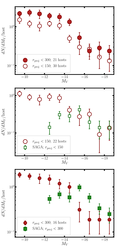
Figure 7: The average satellite abundance per host in 1 mag wide luminosity bins within both $r_{\mathrm{proj}}<150$ and 300 kpc. The legends indicate the number of hosts contributing to each stacked LF. The middle and bottom panels show a comparison to the SAGA Survey (mao2020). Only ELVES hosts that would satisfy the SAGA selection criteria are included. The SAGA Survey LF shows a noticeable drop below $M_{V}>-15$ mag compared to ELVES, even when including a correction for incompleteness in redshift follow-up in that survey.

Figure 7 shows a more detailed look at the ELVES satellite luminosity function (LF). The average differential luminosity function is shown for both $r_{\mathrm{proj}}<150$ and $r_{\mathrm{proj}}<300$ kpc. The unconfirmed candidate satellites are included using their satellite probability values from §5.6. The errorbars show the error in the mean number of satellites per host within each 1 magnitude wide bin. This is calculated as the standard deviation of satellite abundance across the hosts divided by $\sqrt{N_{\mathrm{host}}}$. Thus, these errorbars account for uncertainty coming from the intrinsic host-to-host scatter in satellite abundance. The errorbars are essentially the same as would be calculated from bootstrapping the host sample. Within the errorbars, the average LFs appear to be simple power laws. The $r_{\mathrm{proj}}<300$ kpc LF flattens somewhat at the lowest luminosities, likely due to ELVES starting to lose the lowest surface brightness satellites (cf. Figure 4). The satellite abundance within 150 kpc is generally $\sim 2\times$ lower than that out to 300 kpc.

The middle and bottom panels of Figure 7 show a comparison with the SAGA results. In this comparison, we remove the massive ELVES hosts that would not satisfy the SAGA host $M_{K_{s}}$, isolation, and/or halo mass criteria. The SAGA host $M_{K_{s}}$ requirement ($M_{K_{s}}>-24.6$ mag) removes M104 and M31, the isolation criteria (no satellite with $M_{K_{s}}$ within $1.6$ mag of the host) removes NGC 1808, NGC 5194, NGC 3379, and M81, and the halo mass cut ($M_{h}<10^{13}$ M${}_{\odot}$) removes CenA and NGC 3627. In applying the halo mass cut, we remove any host that has either of the two halo mass estimates provided in the group catalog of kourkchi2017 above $10^{13}$ M${}_{\odot}$. One halo mass estimate comes from group kinematics while the second comes from total $K$-band luminosity. If the two estimates differ by more than $0.5$ dex, we consider the luminosity-based estimate as the more robust. Note that we still include the six ELVES hosts that are actually below SAGA’s host $M_{K_{s}}$ range (NGC 628, NGC 3344, NGC 3556, NGC 4517, NGC 4631, and NGC 4736). There is no change to the conclusions if these are cut as well, albeit the ELVES statistics become poorer. In comparing with SAGA, we additionally only include satellites more than 15 kpc projected from their hosts as this is the estimated inner radial limit of the SAGA satellite lists (Y.-Y. Mao, private communication). The SAGA results make use of our own Sérsic photometry for the SAGA satellites, which we describe below (§LABEL:sec:sat_sf).

In order to account for possible differences in the host $M_{K_{s}}$ distribution even with the SAGA selection criteria applied, we have tried scaling the host abundances to a standard value of $M_{K_{s}}=-23.5$ mag. We use the abundance-$M_{K_{s}}$ relation of font2021 to reduce the weight of more massive hosts and increase the weight of less massive hosts in the average LF stack. We find that this re-scaling has only a minor effect on the average LFs and is thus not shown.

Table 3: Bright vs. faint satellite abundances per host

Radial coverage	Survey	$N_{\mathrm{hosts}}$	$\langle N_{\mathrm{sat}}\rangle$ with $-15<M_{V}<-12$ mag	$\langle N_{\mathrm{sat}}\rangle$ with $-19<M_{V}<-15$ mag
$r_{\mathrm{proj}}<150$ kpc	SAGA	36	0.73$\pm$0.12	0.89$\pm$0.16
	ELVES	22	2.2$\pm$0.31	0.82$\pm$0.2
		(16)	(1.94$\pm$0.37)	(0.56$\pm$0.22)
$r_{\mathrm{proj}}<300$ kpc	SAGA	36	1.82$\pm$0.2	2.15$\pm$0.25
	ELVES	16	3.68$\pm$0.61	0.88$\pm$0.23

Note. — Average number of satellites per host for different radial and luminosity ranges. Note that the ELVES host sample is slightly different between the $r_{\mathrm{proj}}<150$ and $<300$ kpc cases. The values in parentheses give the $r_{\mathrm{proj}}<150$ kpc abundances for the same host sample as in the $r_{\mathrm{proj}}<300$ kpc case. Many of the hosts complete to only 150 kpc are among the richest ELVES hosts.