Quantum Capacities of Transducers

Abstract

High-performance quantum transducers, which can faithfully convert quantum information between disparate physical carriers, are essential elements in quantum science and technology. To assess their ability to coherently transfer quantum information, quantum transducers are typically characterized by different figures of merit including conversion efficiency, bandwidth, and added noise. Here we utilize the concept of quantum capacity, the highest achievable qubit communication rate through a channel, to quantify the performance of a transducer. By evaluating the continuous-time quantum capacity across the conversion band, quantum capacity can serve as a single metric that unifies various desirable criteria of a transducer — high efficiency, large bandwidth, and low noise. Moreover, using the quantum capacities of bosonic pure-loss channels as benchmarks, we investigate the optimal designs of generic quantum transduction schemes implemented by transmitting external signals through a coupled bosonic chain. Under the physical constraint of a bounded maximal coupling rate $g_{\rm max}$, the highest continuous-time quantum capacity $Q^{\rm max}\approx 31.4g_{\rm max}$ is achieved by transducers with a maximally flat conversion frequency response, analogous to Butterworth electric filters. We further extend our method to include thermal noise by considering upper and lower bounds on the quantum capacities of transducers and characterize the performance of maximally flat transducers under the effect of thermal loss.

Introduction

Classically, transducers are devices, such as antenna and microphones, that can convert signal from one physical platform to another. In quantum technology, transducers are essential elements that can faithfully convert quantum information between physical systems with disparate information carriers [Lauk2020, Lambert2020, Han2021]. High-performance quantum transducers are the key to realize quantum networks [Elliott2002, Kimble2008, Komar2014, Simon2017] by interconnecting local quantum processors, such as microwave superconducting systems [Blais2021, Joshi2021], with long-range quantum communication carriers, such as optical fibers [Takesue2015]. Tremendous progress has been made in a variety of coherent platforms for microwave-to-optical [Fan2018, Xu2021, Safavi-Naeini2011, Andrews2014, Higginbotham2018, Hisatomi2016, Zhu2020, Han2020b, Mirhosseini2020, Han2018, Everts2019, Bartholomew2020, Tsuchimoto2021], microwave-to-microwave [Abdo2013, Lecocq2016], and optical-to-optical [Hill2012, DeGreve2012, Lodahl2015] frequency conversion.

Coherent conversion of quantum information between distinct devices is a challenging task. A functional quantum transducer has to satisfy demanding criteria simultaneously — high conversion efficiency, broad bandwidth, and low added noise — and its performance has been characterized by these three figures of merit [Zeuthen2020]. On the other hand, a unified metric to assess the quantum communication capability of transducers is lacking. For example, one transducer may have a high conversion efficiency but operates within a narrow bandwidth, another may allow broadband conversion at a lower efficiency. It is hard to compare their transmission capability given separate criteria.

In this article, we use quantum capacity as a natural metric to characterize the performance of quantum transducers. Quantum capacity is the highest achievable quantum communication rate through a channel [Schumacher1996, Lloyd1997, Devetak2005, Wolf2007]. Here we model direct quantum tranducers as bosonic thermal-loss channels and consider generic conversion process by propagating external signals through a coupled bosonic chain. Using the continuous-time pure-loss quantum capacities of transducers as benchmarks to assess the intrinsic quantum communication capability of transducers, we discover that the optimal designs of transducers are those with maximally flat frequency response around the unity-efficiency conversion peak. Under the physical constraint of a bounded maximal coupling rate $g_{\rm max}$ between the bosonic modes, the maximal continuous-time quantum capacity $Q^{\rm max}\approx 31.4g_{\rm max}$ is achieved by maximally flat transducers implemented by a long bosonic chain. We further include the effect of thermal noise from the environment by considering additive lower and upper bounds on quantum capacities of thermal-loss channels. Our methods provide a unified quantity to assess the performance of transducers across various physical platforms, and suggest a fundamental limit on the quantum communication rate set by the physical coupling strength.

Results

Capacity as a metric for quantum transducers

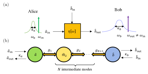
Figure 1: (a) A quantum transducer that can faithfully convert quantum states between different input and output frequencies $\omega_{\rm in}$ and $\omega_{\rm out}$ (in the lab frame), which is modeled as a thermal-loss channel with transmittance $\eta[\omega]$. (b) Schematic of a $N$-stage quantum transducer through a coupled bosonic chain connected to external input and output signals.

We use the concept of quantum capacities of bosonic channels to assess the performance of direct quantum transducers. The quantum capacity quantifies the maximal achievable qubit communication rate through a quantum channel. Here we focus on direct quantum transduction achieved by directly converting quantum signals between bosonic modes via a coherent interface. At a given frequency $\omega$ in the appropriate rotating frame, assuming no intrinsic losses and no amplification gain, a direct quantum transducer with conversion efficiency $\eta[\omega]$ can be modeled as a Gaussian thermal-loss channel [Weedbrook2012] described by the relation between the input and output modes, up to phase shifts,

$$\hat{b}_{\rm out}[\omega] =\sqrt{\eta[\omega]}\hat{a}_{\rm in}[\omega]-\sqrt{1-\eta[\omega]}\hat{b}_{\rm in}[\omega],$$ (1)

where $\hat{a}_{\rm in}[\omega]$ is the input signal mode sent out by Alice, $\hat{b}_{\rm out}[\omega]$ is the output signal mode received by Bob, and $\hat{b}_{\rm in}[\omega]$ is the noisy input state from the environment with a mean thermal photon number $\bar{n}[\omega]=\left\langle\hat{b}_{\rm in}^{\dagger}[\omega]\hat{b}_{\rm in}[\omega]\right\rangle$ (see Fig. 1(a)). Note that we have no access to the reflective signal at Alice’s side.

When the thermal photon number from the environment is negligible, $\bar{n}\approx 0$ for optical systems or via cooling [Lecocq2016, Xu2020], this special case of thermal-loss channels is called the pure-loss channel. For pure-loss channels, their capacities are additive and can be analytically determined. Specifically, for one-way quantum communication (for example, from Alice to Bob only), for discrete-time signals at a given frequency $\omega$ with a fixed conversion efficiency $\eta[\omega]$, the one-way pure-loss capacity is given by [Holevo2001]

$$q_{1}[\omega]=\max\left\{\log_{2}\left(\frac{\eta[\omega]}{1-\eta[\omega]}\right),0\right\},$$ (2)

which is the maximal amount of quantum information that can be reliably transmitted per channel use. This channel has infinite quantum capacity for ideal conversions, $\eta\rightarrow 1$, $q_{1}\rightarrow\infty$, and has vanishing capacity when more than half of the signal is lost, $\eta\in[0,1/2)$, $q_{1}=0$.

In reality, a quantum transducer has a finite conversion band and the conversion efficiency should be frequency-dependent. Treating different frequency modes within the conversion band as parallel quantum channels and taking the continuous limit in $\omega$, here we define a continuous-time one-way pure-loss capacity of a quantum transducer,

$$Q_{1}\equiv\int q_{1}[\omega]d\omega.$$ (3)

In contrast to the discrete-time one-way pure-loss capacity expression Eq. (2) that quantifies the maximal achievable quantum communication rate per channel use, the continuous-time quantum capacity defined in Eq. (3) is the maximal amount of quantum information that can be reliably transmitted through the transducer per unit time. This form of capacity is a direct analog to the Shannon capacity of classical continuous-time communication channels subject to frequency-dependent uncorrelated noises [Gallager1968].

If the pure-loss channel is further assisted by two-way classical communication (between Alice and Bob) and local operations, the corresponding discrete-time two-way pure-loss capacity [Pirandola2017] is given by

$$q_{2}[\omega]=-\log_{2}\left(1-\eta[\omega]\right).$$ (4)

This channel again has infinite quantum capacity for ideal conversions, $\eta\rightarrow 1$, $q_{2}\rightarrow\infty$, but has vanishing capacity only when the efficiency goes to zero, $\eta\rightarrow 0$, $q_{2}=0$. The corresponding continuous-time two-way pure-loss capacity is defined as

$$Q_{2}\equiv\int q_{2}[\omega]d\omega.$$ (5)

The continuous-time pure-loss quantum capacities $Q_{1}$ and $Q_{2}$ defined above incorporate both concepts of efficiency and bandwidth and set the fundamental limit on the quantum communication rate based upon intrinsic transducer properties. We emphasize that $Q_{1}$ and $Q_{2}$ have the unit of qubits per second, and we will show in later text that these highest achievable communication rates are linked to the maximal coupling rates in the underling physical transducer system.

Physical Limit on the Quantum Capacities of Transducers

The conversion efficiency of a transducer, $\eta[\omega]$, is determined by the parameters of its underlying physical implementation. We are interested in how the quantum capacities of transducers $Q_{1}$ and $Q_{2}$ are limited by the physical parameters of the transduction platform. Consider the generic model of direct quantum transducer [Fan2018, Xu2021, Safavi-Naeini2011, Andrews2014, Higginbotham2018, Hisatomi2016, Zhu2020, Han2020b, Mirhosseini2020, Han2018, Everts2019, Bartholomew2020, Tsuchimoto2021, Abdo2013, Lecocq2016, Hill2012] implemented by a coupled bosonic chain with $N$+2 bosonic modes $\hat{m}_{j}$, where the two end modes, $\hat{m}_{1}=\hat{a}$ and $\hat{m}_{N+2}=\hat{b}$, are coupled to external signal input and output ports at rates $\kappa_{1}=\kappa_{a}$ and $\kappa_{N+2}=\kappa_{b}$ respectively (see fig. 1(b)). Coherent quantum conversion can be realized by propagating bosonic signals from mode $\hat{a}$ (at frequency $\omega_{a}$) to mode $\hat{b}$ (at frequency $\omega_{b}$) through $N$ intermediate stages, and we call this interface a $N$-stage quantum transducer. The conversion efficiency of a $N$-stage transducer is a frequency-dependent function determined by system parameters [Xu2021, Wang2022],

$$\eta_{N}=\eta_{N}[\omega](\kappa_{a},\kappa_{b},\left\{\Delta_{j}\right\},\left\{g_{j}\right\}),$$ (6)

where $\Delta_{j}$ is the detuning of mode $\hat{m}_{j}$ in the rotating frame of the laser drive(s) that bridges the up- and down-conversions between the input and output signals, and $g_{j}$ is the coupling strength of the beam-splitter type interaction between the neighboring bosonic pair $\hat{m}_{j}$ and $\hat{m}_{j+1}$. Here we have assumed the system has no intrinsic losses and we will take $g_{j}$’s to be real and positive without loss of generality.

For realistic physical implementations, the coherent coupling between neighboring modes is typically the most demanding resource. Therefore, under the physical constraint $\forall j,g_{j}\leq g_{\rm max}$, we look for the optimized choice of parameters $\kappa_{a}$, $\kappa_{b}$, $\Delta_{j}$’s, and $g_{j}$’s to achieve the maximal possible $Q_{1}$ and $Q_{2}$ for $N$-stage quantum transducers. To attain the highest possible capacity, the physical parameters of the transducer have to satisfy the generalized matching condition [Wang2022] such that $\eta_{N}[\omega_{c}]=1$ at some frequency $\omega_{c}$. Note that the physics of the system is invariant under an overall shift in energy by choosing a different rotating frame, which corresponds to the relocation of $\omega_{c}$.

Using the continuous-time pure-loss capacities as the benchmarks, we find that maximal values of $Q_{1}$ and $Q_{2}$ are achieved when the $N$-stage quantum transducer has a maximally flat (MF) efficiency,

$$\left.\frac{\partial\eta^{\rm MF}_{N}[\omega]}{\partial\omega}\right|_{\omega=\omega_{c}}=\cdots=\left.\frac{\partial^{2N+3}\eta^{\rm MF}_{N}[\omega]}{\partial\omega^{2N+3}}\right|_{\omega=\omega_{c}}=0.$$ (7)

Intuitively, with a flat plateau around $\eta_{N}[\omega_{c}]=1$, this maximally flat transducer design guarantees a local maximum for $Q_{1}$ and $Q_{2}$, and we have seen strong numerical evidence that this solution is likely a global maximum as well under the physical constraint $\forall j,g_{j}\leq g_{\rm max}$ (see Methods). In the later discussion, we will use this as an optimized design for $N$-stage transducers. For $N$-stage transducers under the above physical constraint, we find that the optimal parameters satisfying Eq. (7), denoted by ${}^{\star}$, are

$$\kappa^{\star}_{a}=\kappa^{\star}_{b}=2\sqrt{\frac{\sin\left[\tfrac{3\pi}{2(N+2)}\right]}{\sin\left[\tfrac{\pi}{2(N+2)}\right]}}g_{\rm max},$$ (8)

$$g^{\star}_{j}=\sqrt{\frac{\sin\left[\tfrac{\pi}{2(N+2)}\right]\sin\left[\tfrac{3\pi}{2(N+2)}\right]}{\sin\left[\tfrac{(2j-1)\pi}{2(N+2)}\right]\sin\left[\tfrac{(2j+1)\pi}{2(N+2)}\right]}}g_{\rm max},$$ (9)

and $\forall j,\Delta^{\star}_{j}=-\omega_{c}$ (see Methods). Note that the optimized parameters are symmetric, $g^{\star}_{j}=g^{\star}_{N+2-j}$, $\kappa^{\star}_{a}=\kappa^{\star}_{b}$, and $g^{\star}_{1}=g^{\star}_{N+1}=g_{\rm max}$.

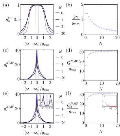
Figure 2: Diagrams for $N$-stage quantum transducers with maximally flat conversion efficiency. (a) Maximally flat efficiency function $\eta^{\rm MF}_{N}[\omega]$ for different $N$. (b) The mean coupling $\bar{g}_{N}$ as a function of $N$. (c) The discrete-time one-way pure-loss capacity, $q^{N,\rm MF}_{1}[\omega]$, for different $N$. (d) The continuous-time one-way pure-loss capacity, $Q^{N,\rm MF}_{1}$, as a function of $N$. (e) The discrete-time two-way pure-loss capacity, $q^{N,\rm MF}_{2}[\omega]$, for different $N$. Inset shows the gain in capacity assisted by the two-way protocol, $q^{N,\rm MF}_{2}[\omega]-q^{N,\rm MF}_{1}[\omega]$. (f) The continuous-time two-way pure-loss capacity, $Q^{N,\rm MF}_{2}$, as a function of $N$. Inset shows the gain in capacity assisted by the two-way protocol, $(Q^{N,\rm MF}_{2}-Q^{N,\rm MF}_{1})/g_{\rm max}$.

A $N$-stage maximally flat transducer is a direct analog to a ($N+2$)-th order Butterworth low-pass electric filter (see Methods). The maximally flat efficiency $\eta_{N}^{\rm MF}[\omega]$ has a general form

$$\eta^{\rm MF}_{N}[\omega]=\frac{1}{((\omega-\omega_{c})/\bar{g}_{N})^{2(N+2)}+1},$$ (10)

where

$$\bar{g}_{N}\equiv 2\sqrt{\sin\left[\tfrac{\pi}{2(N+2)}\right]\sin\left[\tfrac{3\pi}{2(N+2)}\right]}g_{\rm max}.$$ (11)

Here $\bar{g}_{N}$ is the mean coupling given by $\bar{g}_{N}=\sqrt[N+2]{\sqrt{\kappa^{\star}_{a}\kappa^{\star}_{b}}\prod_{j=1}^{N+1}g^{\star}_{j}}$, and it also has the physical meaning of the transducer bandwidth — the full width at half maximum of $\eta^{\rm MF}_{N}[\omega]$ is 2$\bar{g}_{N}$. The value of $\bar{g}_{N}/g_{\rm max}$ monotonically decreases with $N$ as shown in Fig. 2(b) .

Given this general form, we can find their discrete-time pure-loss capacities at a given frequency, $q^{N,\rm MF}_{1}[\omega]$ and $q^{N,\rm MF}_{2}[\omega]$, and then evaluate the continuous-time pure-loss capacities of the maximally flat transducers (see Fig. 2(c)-(f)). Specifically,

$$Q_{1}^{N,\rm MF}=\frac{4(N+2)}{\log(2)}\bar{g}_{N},$$ (12)

$$Q_{2}^{N,\rm MF}=\frac{2\pi}{\log(2)\sin\left[\tfrac{\pi}{2(N+2)}\right]}\bar{g}_{N},$$ (13)

for one-way and two-way protocols respectively. At large $N$, the continuous-time pure-loss quantum capacities saturate to the same value

$$\lim_{N\rightarrow\infty}Q_{1}^{N,\rm MF}=\lim_{N\rightarrow\infty}Q_{2}^{N,\rm MF}\equiv Q^{\rm max}=\frac{4\sqrt{3}\pi}{\log(2)}g_{\rm max}.$$ (14)

The above expression represents a physical limit on the maximal achievable quantum communication rate through a transducer, $Q^{\rm max}\approx 31.4g_{\rm max}$ (qubit/sec). The quantum communication rate through a transducer is limited by the maximal available coupling strength within the bosonic chain.

We now compare the performance of the maximally flat transducer to uniformly coupled transducers with $\forall j,\tilde{g}_{j}=g_{\rm max}$, $\tilde{\Delta}_{j}=-\omega_{c}$, and $\tilde{\kappa}_{a}=\tilde{\kappa}_{b}=2g_{\rm max}$ for even $N$, and $\tilde{\kappa}_{a}=\tilde{\kappa}_{b}=2\sqrt{\frac{N+3}{N+1}}g_{\rm max}$ for odd $N$ (see Methods).

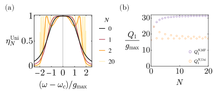
Figure 3: (a) Optimal efficiency function $\eta^{\rm Uni}_{N}[\omega]$ for $N$-stage transducers with uniform couplings. (b) Continuous-time one-way pure-loss quantum capacities of $N$-stage maximally flat transducers (purple) and uniform transducers (orange).

The optimal efficiency functions for $N$-stage uniform transducers are shown in Fig. 3(a) and their continuous-time one-way pure-loss capacities, $Q^{N,\rm Uni}_{1}$, as a function of $N$ are shown in orange in Fig. 3(b). One can see that a $N$-stage maximally flat transducer may transmit about twice amount of quantum information per unit time compared to a $N$-stage uniform transducer with a uniform coupling rate $g_{\rm max}$. The achievable quantum communication rate is even lower for arbitrary transducer parameters without flatness features around $\eta[\omega_{c}]=1$.

Transducers under thermal noise

For realistic transduction schemes within a noisy environment, the quantum capacity will decrease due to the effect of thermal noise. The quantum capacities of Gaussian thermal-loss channels have yet to be analytically determined, but we can approach their values using additive upper and lower bound expressions. We now extend the continuous-time quantum capacity for thermal-loss channels with non-zero $\bar{n}$ . For one(two)-way scenario, we can define the continuous-time one(two)-way thermal-loss capacity lower(upper) bound for transducers as

$$Q_{1(2),\bar{n},L(U)}\equiv\int q_{1(2),\bar{n},L(U)}[\omega]d\omega,$$ (15)

where $q_{1(2),\bar{n},L(U)}$ is the discrete-time one(two)-way thermal-loss capacity lower(upper) bound (see Methods).

The continuous-time quantum capacities of maximally flat transducers with different mean thermal photon numbers are shown in Fig. 4. One can see that the quantum capacities of maximally flat transducers are less susceptible to thermal loss at large $N$, and the difference between the upper and lower bounds also vanishes at large $N$ (see Methods for analytical expansions).

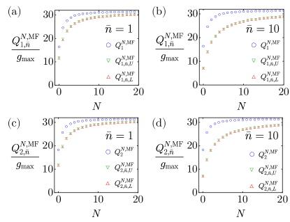
Figure 4: Quantum capacities of maximally flat transducers under thermal loss. (a) Continuous-time one-way thermal-loss capacity upper and lower bounds with mean thermal photon number $\bar{n}=1$. (b) Continuous-time one-way thermal-loss capacity upper and lower bounds with mean thermal photon number $\bar{n}=10$. (c) Continuous-time two-way thermal-loss capacity upper and lower bounds with mean thermal photon number $\bar{n}=1$. (d) Continuous-time two-way thermal-loss capacity upper and lower bounds with mean thermal photon number $\bar{n}=10$. We also show the pure-loss capacities $Q_{1}^{N,\rm MF}$ and $Q_{2}^{N,\rm MF}$ corresponding to $\bar{n}=0$ for comparison.

Discussion

We have used the continuous-time quantum capacities to characterize the performance of direct quantum transducers. By considering the generic physical model of an externally connected bosonic chain with a bounded coupling rate $g_{\rm max}$, we showed that the maximal qubit communication rate of a transducer is given by $Q^{\rm max}\approx 31.4g_{\rm max}$. Such maximal capacity is achieved by maximally flat $N$-stage quantum transducers with $N\rightarrow\infty$. Note that our result has no contradiction to the Lieb-Robinson bound [Lieb1972] — after signals arrive at a delayed time, increasing with $N$ as predicted by Lieb and Robinson, the qubit communication rate is upper-bounded by the quantum capacity of the transducer that saturates to a finite value $Q^{\rm max}$ at large $N$ in the optimal scenario.

This work provides a fundamental limit of transducer capacities in terms of coupling strength, and offers a quantitative comparison for direct transducers across platforms that consolidates distinct metrics of efficiency, bandwidth, and added thermal noise. Our method can be directly extended to transducers with intrinsic losses by considering the dependence of the conversion efficiency $\eta_{N}$ on the intrinsic dissipation rates [Xu2021, Wang2022]. Intriguing future works include exploring bosonic encodings, such as GKP codes [Gottesman2001], to approach the quantum capacity bound and investigating superadditivity of general quantum capacities. Here we have focused on direct transducers that can be well-modeled as a Gaussian thermal-loss channel with neither amplification gain nor access to the reflective signal. A more general framework incorporating disparate transduction schemes, like direct transduction with amplification due to extra two-mode squeezing couplings, or entanglement-based [Zhong2020a, Wu2021, Zhong2022], adaptive-based [Zhang2018], and interference-based [Lau2019, Zhang2020] transductions that involve the reflective signal, is left as an open frontier to be explored.

Methods

Conversion Efficiency of $N$-stage Quantum Transducers

The conversion efficiency of a $N$-stage transducer without intrinsic loss is given by [Wang2022]

$$\eta_{N}[\omega]=\absolutevalue{\frac{\sqrt{\kappa_{a}\kappa_{b}}\prod_{j=1}^{N+1}g_{j}}{D_{N}[\omega]}}^{2},$$ (16)

where $D_{N}[\omega]$ is the determinant of a ($N$-2) $\times$ ($N$-2) tridiagonal matrix

$$D_{N}[\omega]\equiv\begin{vmatrix}\chi_{a}^{-1}&ig_{1}&0&\cdots&\cdots&0\\ ig_{1}&\chi_{2}^{-1}&ig_{2}&\ddots&&\vdots\\ 0&ig_{2}&\ddots&\ddots&\ddots&\vdots\\ \vdots&\ddots&\ddots&\ddots&\ddots&0\\ \vdots&&\ddots&\ddots&\ddots&ig_{N+1}\\ 0&\cdots&\cdots&0&ig_{N+1}&\chi_{b}^{-1}\end{vmatrix}.$$ (17)

Here $\chi_{j}=(i(\omega+\Delta_{j})+\kappa_{j}/2)^{-1}$ is the susceptibility of mode $\hat{m}_{j}$, with $\kappa_{1}=\kappa_{a}$, $\kappa_{N+2}=\kappa_{b}$, and $\kappa_{j}=0$ otherwise.

Physical Parameters of Maximally Flat Transducers

In this section we will prove that the optimal parameters given in Eq. (8&9) give rise to maximally flat efficiency for transducers. Consider a ($N$-2) $\times$ ($N$-2) tridiagonal matrix $F_{N+2}$ defined as

(18)

(19)

(20)

(21)

(22)

Thegenerali