Path-integral Monte Carlo worm algorithm for Bose systems
with periodic boundary conditions

Abstract

We provide a detailed description of the path-integral Monte Carlo worm algorithm used to exactly calculate the thermodynamics of Bose systems in the canonical ensemble. The algorithm is fully consistent with periodic boundary conditions, that are applied to simulate homogeneous phases of bulk systems, and it does not require any limitation in the length of the Monte Carlo moves realizing the sampling of the probability distribution function in the space of path configurations. The result is achieved adopting a representation of the path coordinates where only the initial point of each path is inside the simulation box, the remaining ones being free to span the entire space. Detailed balance can thereby be ensured for any update of the path configurations without the ambiguity of the selection of the periodic image of the particles involved. We benchmark the algorithm using the non-interacting Bose gas model for which exact results for the partition function at finite number of particles can be derived. Convergence issues and the approach to the thermodynamic limit are also addressed for interacting systems of hard spheres in the regime of high density.

I Introduction

The path-integral Monte Carlo (PIMC) method is a computational approach that allows one to exactly calculate the equilibrium properties of Bose systems at finite temperature starting from the microscopic Hamiltonian. The first applications of the method addressed the study of bulk liquid and solid ⁴He approaching the quantum degenerate regime [1, 2]. Similarly to these first simulations, many later implementations of the PIMC algorithm addressed homogeneous systems featuring infinite spatial extension in the physically relevant dimensions. To mimic such configurations, the use of periodic boundary conditions in the computer simulations is crucial [3]. The size of the simulation cell enters as an important parameter of the numerical procedure, calling for a careful extrapolation of all the results to a properly defined thermodynamic limit. Another crucial aspect of PIMC simulations is the efficient sampling of Bose-particle permutations. This gets increasingly important with the level of quantum degeneracy and is essential to obtain reliable estimates of observables such as the superfluid density and the condensate fraction [4, 5]. In this context, an important technical advancement emerged with the introduction of the worm algorithm, first devised for lattice models [6, 7] and later extended to continuous-space simulations [8, 9]. The PIMC method implementing the worm algorithm has proven to be one of the most powerful computational quantum many-body techniques. It allowed performing accurate simulations of intriguing phenomena in different condensed matter systems, such as dipolar systems [10, 11, 12], ultracold gases [13, 14, 15, 16, 17] and quantum fluids and solids [18, 19, 20, 21, 22, 23, 24]. However, the original implementation of the worm algorithm is not fully compatible with periodic boundary conditions. This can lead to biased results when the de Broglie thermal wavelength starts to be comparable to the size of the fundamental periodic cell. The basic idea behind the worm algorithm is the use of both diagonal and off-diagonal configurations of the paths describing particles in the many-body system. Various moves of portions of the paths are devised to ensure the ergodic sampling of both types of configurations as well as to switch from the diagonal to the off-diagonal sector and vice-versa. Such moves, satisfying detailed balance, have a straightforward implementation in the case of a system with infinite extension or of a confined finite geometry. In periodic systems, instead, the ambiguity in the choice of periodic images might lead to biased results, unless stringent constraints are imposed on the portions of the paths involved in certain Monte Carlo moves. Such bias can be avoided by adopting periodic cells much larger than the thermal wavelength, but this becomes impractical in the zero temperature limit. Furthermore, the limitations in the updates can affect the efficiency of the Monte Carlo sampling. We present here a formalism and a detailed recipe for a PIMC algorithm for bosons in the canonical ensemble which is rigorously compatible with periodic boundary conditions. With this algorithm, no constraint has to be imposed on the Monte Carlo updates, even for small periodic cells. We use as a benchmark the canonical non-interacting Bose gas in a periodic box for which exact results for the energy can be obtained for any number of particles in the box. Direct comparison with these results permits us to check one by one the various elementary moves of our novel implementation of the worm algorithm, verifying that they provide an unbiased ergodic sampling. Interacting systems are considered only with the hard-sphere model interaction and the pair-product approximation. In this case, no exact result is available for finite box-like geometries even for just a pair of particles. Nonetheless, we can investigate the convergence of the results for a given number of particles in terms of the length of the path steps in imaginary time as well as the approach to the thermodynamic limit when the number of particles in the simulation is increased.

The structure of the paper is as follows. In section II we introduce the representation of the particle coordinates consistent with the use of periodic boundary conditions. Trying to be pedagogical we first consider the case of a single particle in a one-dimensional periodic box and then move to the case of $N$ identical particles. In the same section we describe the general scheme of the worm algorithm and we introduce in details the various Monte Carlo updates. In section III we benchmark the algorithm against exact results of the non-interacting Bose gas for one, two and many particles at different temperatures. Section IV is devoted to interacting systems for which we use the hard-sphere model in the regime of high density. We address the convergence of the algorithm for a given number of particles $N$ and for different temperatures as well as the approach to the thermodynamic limit. Finally in the last section we draw our conclusions. In the appendix we outline the useful formulas used for the calculation of the internal energy, both the thermodynamic and virial estimator, and of the pressure.

II Path Integral Monte Carlo

In a PIMC simulation one aims at calculating the partition function $Z_{N}$ of a Bose system of $N$ identical particles described by the Hamiltonian $H$ and with inverse temperature $\beta=1/(k_{B}T)$, where $k_{B}$ is Boltzmann’s constant. In the coordinate representation, the partition function is defined as the trace over all states $|\bm{\mathrm{R}}\rangle$ of the density matrix $\rho(\bm{\mathrm{R}},\bm{\mathrm{R}}^{\prime},\beta)=\langle\bm{\mathrm{R}}|e^{-\beta H}|\bm{\mathrm{R}}^{\prime}\rangle$ properly symmetrized,

$$Z_{N}=\frac{1}{N!}\sum_{P}\int d\bm{\mathrm{R}}\,\rho(\bm{\mathrm{R}},P\bm{\mathrm{R}},\beta)\;.$$ (1)

Here, $\bm{\mathrm{R}}=(\bm{\mathrm{r}}_{1},\bm{\mathrm{r}}_{2},...,\bm{\mathrm{r}}_{N})$ collectively denotes the position vectors of the particles and $P\bm{\mathrm{R}}=(\bm{\mathrm{r}}_{p(1)},\bm{\mathrm{r}}_{p(2)},...,\bm{\mathrm{r}}_{p(N)})$ corresponds to the position vectors with permuted labels. Furthermore, the sum in the above equation extends over the $N!$ permutations of the particle labels. The partition function can be conveniently rewritten in terms of the convolution integral

$$Z_{N}=\frac{1}{N!}\sum_{P}\int d\bm{\mathrm{R}}\int d\bm{\mathrm{R}}_{1}\dots\int d\bm{\mathrm{R}}_{M-1}\,\rho(\bm{\mathrm{R}},\bm{\mathrm{R}}_{1},\delta_{\tau})\dots\rho(\bm{\mathrm{R}}_{M-1},P\bm{\mathrm{R}},\delta_{\tau})\;,$$ (2)

where $\delta_{\tau}=\beta/M$. Starting from the above decomposition, the calculation is mapped to a classical-like simulation of polymeric chains with a number of beads $M$ equal to the number of terms of the convolution integral. More specifically, one makes use of suitable approximations for the density matrix $\rho(\bm{\mathrm{R}},\bm{\mathrm{R}}^{\prime},\delta_{\tau})$ at the higher temperature $1/\delta_{\tau}$ and performs the multidimensional integration over $\bm{\mathrm{R}},\bm{\mathrm{R}}_{1},\dots,\bm{\mathrm{R}}_{M-1}$ as well as the sum over permutations $P$ by Monte Carlo sampling [1, 2]. The whole procedure can be unambiguously followed if the particle coordinates $\bm{\mathrm{r}}_{1},\dots,\bm{\mathrm{r}}_{N}$ can span the entire space, for example when the Hamiltonian includes a confining external potential. In the case of interest of a bulk system, where the simulation cell corresponds to a box periodically replicated in space, the coordinates $\bm{\mathrm{r}}_{i}$ can either denote the position of the $i$-th particle in the box or of one of its periodic images in the neighboring boxes. This ambiguity has troublesome consequences in the proper sampling of configurations $\bm{\mathrm{R}}$ with the correct probability distribution. In particular, a naïve implementation of the Monte Carlo updates might lead to the violation of the detailed balance condition. In the following subsection we motivate the use of a specific representation for the particle coordinates that allows one to unambiguously construct a PIMC algorithm that is consistent with periodic boundary conditions. The upshot is that one should consider coordinates as belonging to the infinite space throughout the whole simulation, and invoke periodic boundary conditions only when considering the periodicity of the trajectories in imaginary time or the interaction among different particles. First, we consider the simplest possible example, namely a single particle in one dimension, to show how this coordinate representation naturally emerges in the context of the path-integral representation of the partition function. Once the single particle case has been clarified, we extend the formalism to the $N$-body system with periodic boundary conditions.

II.1 Path Integral for one particle with periodic boundary conditions

We consider a particle moving on a circle $\mathcal{S}^{1}\sim\mathbb{R}~{}/~{}\mathbb{Z}$ of length $L$ whose momentum is quantized in units of $2\pi\hbar/L$. A position eigenstate on the circle can be represented as the Fourier series

$$\ket{x}_{\mathcal{S}^{1}}=\frac{1}{\sqrt{L}}\sum_{n=-\infty}^{\infty}e^{-\dfrac{ip_{n}x}{\hbar}}\ket{p_{n}}\,,\qquad p_{n}=\frac{2\pi\hbar}{L}n\,,$$ (3)

but it can also be expressed as the superposition of eigenstates in the space $\mathbb{R}$ as

$$\ket{x}_{\mathcal{S}^{1}}=\sqrt{\frac{L}{2\pi\hbar}}\sum_{n=-\infty}^{\infty}\ket{x+nL}\,.$$ (4)

In the above equations the coordinate $x$ is limited to the fundamental cell $[0,L)$ and we used the notation $\ket{}_{\mathcal{S}^{1}}$ to represent a state on ${\mathcal{S}^{1}}$ while with the standard ket $\ket{}$, without subscripts, we represented a state on the real line $\mathbb{R}$. For later convenience we introduce the following alternative labeling of the states on $\mathbb{R}$:

$$\ket{x+nL}\equiv\ket{x,n}\,,$$ (5)

which explicitly separates the coordinate in the fundamental cell from the integer identifying one of the periodic images. The momentum eigenstate $\ket{p_{n}}$ does not have this distinction since the plane-wave decomposition can equivalently be expressed in the two spaces as

$$\ket{p_{n}}=\frac{1}{\sqrt{L}}\int_{0}^{L}dx\,e^{\dfrac{ip_{n}x}{\hbar}}\ket{x}_{\mathcal{S}^{1}}=\frac{1}{\sqrt{2\pi\hbar}}\int_{-\infty}^{\infty}dx\,e^{\dfrac{ip_{n}x}{\hbar}}\ket{x}\,.$$ (6)

We can then write the partition function of a free particle of mass $m$ in one dimension with periodic boundary conditions using the set of coordinates on the real line $\mathbb{R}$:

$$Z_{1}=\int_{0}^{L}dx\,\sum_{n=-\infty}^{\infty}\bra{x,0}e^{-\dfrac{\beta p^{2}}{2m}}\ket{x,n}\,,$$ (7)

where $p$ is the momentum operator. Notice that the above equation computes the trace over the Boltzmann factors by fixing a reference in the fundamental cell and then summing over all periodic images. The reader can easily verify that the above expression evaluates to the same result as the more familiar formula $Z_{1}=\sum_{n}\exp[-\beta p_{n}^{2}/(2m)]$. It is also important to notice that if one limits to $n=0$ the summation over images in eq. (7), i.e. only the particle in the simulation box is considered, the result for $Z_{1}$ would be correct only in the limit $\lambda_{T}\ll L$, where $\lambda_{T}=\sqrt{2\pi\hbar^{2}\beta/m}$ is the thermal wavelength. For the particular example of a single particle in a box, this issue explains the difficulty of a path-integral algorithm with periodic boundary conditions [3]. We can then define $\delta_{\tau}=\beta/M$, with $M$ being a positive integer, and introduce $M-1$ completeness relations on the real line $\mathbb{R}$,

$$1=\int_{-\infty}^{\infty}dx\,\ket{x}\bra{x}\,,$$ (8)

to obtain a representation of $Z_{1}$ suitable for a PIMC simulation:

$$Z_{1}=\int_{0}^{L}dx\,\sum_{n=-\infty}^{\infty}\int_{-\infty}^{\infty}dx_{1}\dots dx_{M-1}\,\bra{x,0}e^{-\frac{\delta_{\tau}p^{2}}{2m}}\ket{x_{1}}\bra{x_{1}}\dots\ket{x_{M-1}}\bra{x_{M-1}}e^{-\frac{\delta_{\tau}p^{2}}{2m}}\ket{x,n}\,.$$ (9)

Notice that the expression above involves a product of matrix elements obtained from states defined on the real line $\mathbb{R}$. The periodicity of the space just constrains the leftmost bra to span the fundamental cell, and the rightmost ket to coincide with one of the images labeled by $n$. Before moving to the more general case of a system of $N$ particles in $D$-dimensions, let us introduce the analog of the partition function in eq. (7) for non-diagonal (or two-point) configurations,

$$G_{1}=\frac{1}{L}\int_{0}^{L}dx^{\prime}\int_{0}^{L}dx\,\sum_{n=-\infty}^{\infty}\bra{x,0}e^{-\dfrac{\beta p^{2}}{2m}}\ket{x^{\prime},n}\,,$$ (10)

where the matrix element is between a state in the fundamental cell and a generic other state. This quantity will characterize the simulation in the off-diagonal sector and it can be rewritten as

$$G_{1}=\frac{1}{L}\int_{-\infty}^{\infty}dx^{\prime}\int_{0}^{L}dx\,\bra{x,0}e^{-\dfrac{\beta p^{2}}{2m}}\ket{x^{\prime}}\,.$$ (11)

The generalizations of eqs. (7) and (11) to the $D$-dimensional $N$-particle system, in which the paths of the particles in imaginary time are represented on the infinite space, with only one reference coordinate in the fundamental cell, provides an unambiguous parametrization of the PIMC method and will be employed below to construct a worm algorithm that is consistent with periodic boundary conditions.

II.2 Path Integral for $N$ bosons with periodic boundary conditions

We consider now a system composed of $N$ identical bosons of mass $m$ contained in a $D$-dimensional hypercube of volume $V=L^{D}$. The use of periodic boundary conditions makes the space of coordinates the $D$-dimensional torus $(\mathbb{R}~{}/~{}\mathbb{Z})^{D}$. Generalizing the notation of the previous subsection, we introduce the coordinates inside the box $\bm{\mathrm{X}}=(\bm{\mathrm{x}}_{1},\bm{\mathrm{x}}_{2},\dots,\bm{\mathrm{x}}_{N})$, with $\bm{\mathrm{x}}_{i}\in[0,L)^{D}$, and a collection of integers ${\bm{\mathrm{W}}}=({\bm{\mathrm{w}}}_{1},{\bm{\mathrm{w}}}_{2},\dots,{\bm{\mathrm{w}}}_{N})$, with ${\bm{\mathrm{w}}}_{i}\in\mathbb{Z}^{D}$ labeling the image of the $i$-th particle. An $N$-particle state can then be defined as

$$\ket{\bm{\mathrm{R}}=\bm{\mathrm{X}}+{\bm{\mathrm{W}}}L}\equiv\ket{\bm{\mathrm{X}},{\bm{\mathrm{W}}}}\,.$$ (12)

The partition function can then be written as

$$Z_{N}=\frac{1}{N!}\sum_{P}\sum_{\bm{\mathrm{W}}}\int_{V}\;d\bm{\mathrm{X}}\,\bra{\bm{\mathrm{X}},\bm{\mathrm{0}}}e^{-\beta H}\ket{P\bm{\mathrm{X}},{\bm{\mathrm{W}}}}\,,$$ (13)

where $P\bm{\mathrm{X}}=(\bm{\mathrm{x}}_{p(1)},\bm{\mathrm{x}}_{p(2)},\dots,\bm{\mathrm{x}}_{p(N)})$ indicates the position vector in the box $V$ with permuted indices. By using the convolution rule and introducing $M-1$ intermediate beads each at the inverse temperature $\delta_{\tau}=\beta/M$, the partition function can be written as

$$Z_{N}=\frac{1}{N!}\sum_{P}\int\prod_{j=0}^{M-1}d\bm{\mathrm{R}}_{j}\,\rho(\bm{\mathrm{R}}_{j},\bm{\mathrm{R}}_{j+1},\delta_{\tau})\,,\qquad\bm{\mathrm{R}}_{M}\equiv P\bm{\mathrm{X}}_{0}+{\bm{\mathrm{W}}}L\,.$$ (14)

In the above equation we have combined the integration over $\bm{\mathrm{X}}_{0}$ and the sum over the integers ${\bm{\mathrm{W}}}$ into an integration over $\bm{\mathrm{R}}_{0}$, and implicitly required that the vector $\bm{\mathrm{R}}_{0}$ appearing as the argument of the density matrix has to be considered as the image in the fundamental cell, i.e. the vector $\bm{\mathrm{X}}_{0}$. Similarly to the one-dimensional case in the previous subsection, the remaining vectors $\bm{\mathrm{R}}_{1},\dots,\bm{\mathrm{R}}_{M}$, span the entire space. As previously stated, in a PIMC calculation one performs a classical-like simulation of polymers formed by $M$ links, connecting $M+1$ beads. Each polymer corresponds to one boson, that can close on itself (if $p(i)=i$) or on another particle specified by the permutation index $p(i)$. Notice that each polymer $i$ starts at the bead $0$ inside the fundamental cell, and ends at bead $M$, closing on an image of the first bead of the polymer $p(i)$, identified up to the periodicity of the $D$-dimensional torus. Denoting with $X$ a configuration of the $N$ particles (that will be defined more in detail later), one can see that eq. (14) naturally provides a probability density function (PDF), given by

$$\pi(X)=\frac{1}{Z_{N}}\frac{1}{N!}\prod_{j=0}^{M-1}\rho(\bm{\mathrm{R}}_{j},\bm{\mathrm{R}}_{j+1},\delta_{\tau})\,,$$ (15)

that can be sampled using the Metropolis–Hastings algorithm [25, 26]. Diagonal thermodynamic observables can then be directly computed using the above PDF from the configurations visited by the simulation. With obvious notation, the equilibrium statistical average of a given operator $O$ is given by

$$\braket{O}=\int\mathcal{D}X\,\pi(X)O(X)\,.$$ (16)

For the systems that are considered here, the Hamiltonian can be expressed as the sum $H=\mathcal{T}+\mathcal{V}$ of a quadratic kinetic part $\mathcal{T}=\sum_{i}p_{i}^{2}/(2m)$, with $p_{i}$ being the momentum operator associated to particle $i$, and a potential part $\mathcal{V}$, usually diagonal in the coordinate representation. In such a case, for sufficiently large $M$ an accurate approximation of the high-temperature density matrices is ensured by the Trotter product formula [27]

$$e^{-\beta(\mathcal{T}+\mathcal{V})}=\lim_{M\to\infty}\left[e^{-\delta_{\tau}\mathcal{T}}e^{-\delta_{\tau}\mathcal{V}}\right]^{M}\,,$$ (17)

allowing us to rewrite the density matrices appearing in eq. (15) as

$$\rho(\bm{\mathrm{R}}_{j},\bm{\mathrm{R}}_{j+1},\delta_{\tau})=\rho_{\mathrm{free}}(\bm{\mathrm{R}}_{j},\bm{\mathrm{R}}_{j+1},\delta_{\tau})\exp{\left[-U(\bm{\mathrm{R}}_{j},\bm{\mathrm{R}}_{j+1})\right]}\,,$$ (18)

where $U$ is the potential energy term, while $\rho_{\mathrm{free}}$ is the free particle density matrix obtained from the kinetic operator

$$\rho_{\mathrm{free}}(\bm{\mathrm{R}}_{j},\bm{\mathrm{R}}_{j+1},\delta_{\tau})\equiv\prod_{i=1}^{N}\rho_{\mathrm{free}}^{\mathrm{sp}}(\bm{\mathrm{r}}_{i,j},\bm{\mathrm{r}}_{i,j+1},\delta_{\tau})=\prod_{i=1}^{N}(4\pi\lambda\delta_{\tau})^{-D/2}\exp\left[-\frac{(\bm{\mathrm{r}}_{i,j}-\bm{\mathrm{r}}_{i,j+1})^{2}}{4\lambda\delta_{\tau}}\right]\,,$$ (19)

with $\lambda=\hbar^{2}/(2m)$. In the so-called symmetrized primitive approximation the potential energy term is given by $U(\bm{\mathrm{R}}_{j},\bm{\mathrm{R}}_{j+1})=\delta_{\tau}\left(\mathcal{V}(\bm{\mathrm{R}}_{j})+\mathcal{V}(\bm{\mathrm{R}}_{j+1})\right)/2$. Depending on the problem at hand, one might significantly reduce the number $M$ of slices needed for convergence using different approximation schemes. An effective scheme in the case of dilute systems with hard-sphere interaction is the pair-product ansatz [3]. This is discussed in more detail in section IV. Let us anticipate that the factorization of eq. (18) highlights the possibility of using efficient strategies to exactly sample the free Gaussian part $\rho_{\mathrm{free}}$, leaving the acceptance/rejection stage of the Metropolis–Hastings algorithm to be determined only by the potential interaction term. Among the possible schemes we adopt the staging algorithm [28, 29], a smart collective displacement of an arbitrary number of beads.

II.3 Worm algorithm

The configuration space detailed above, which will be called $Z$-sector in what follows, consists of polymers organized by the permutation vector $P$ into a number of cycles, i.e. subsets with cyclic permutations, meaning that each polymer has links connecting it to a preceding and a following polymer. Instead of directly summing the $N!$ integrals corresponding to just as many permutations, we use a Monte Carlo integration strategy based on the worm algorithm [30, 6, 7, 8, 9], which is based on an extended configuration space where the $Z$-sector is augmented by a $G$-sector, obtained by cutting one of the cycles and leaving one sequence open-ended. This open sequence of polymers constitutes the worm, with the first polymer called the tail and the last one called the head. During the simulation, the system randomly fluctuates between the two sectors by opening or closing the worm and, when in the $G$-sector, the head of the worm might be swapped with another polymer, thus sampling the permutations and allowing the creation of long permutation cycles. Configurations in the $G$-sector are obtained from a configuration in the $Z$-sector complemented by a particle index $i_{H}$, indicating the head of the worm, and an extra position vector, $\bm{\mathrm{r}}_{i_{H},M}=\bm{\mathrm{x}}_{H}+{\bm{\mathrm{w}}}_{i_{H}}L$, representing an additional bead at the head of the worm dangling at the time slice $j=M$. We need this additional position vector because we want the PDF in the $G$-sector to be the analogue of the one in the $Z$-sector, thus requiring the same total number of links. We can now define the analogue of the partition function in the $G$-sector as

$$G_{N}=\frac{1}{VN!}\sum_{P}\sum_{i_{H}=1}^{N}\int_{V}\;d\bm{\mathrm{x}}_{H}\int\prod_{j=0}^{M-1}d\bm{\mathrm{R}}_{j}\,\rho(\bm{\mathrm{R}}_{j},\bm{\mathrm{R}}_{j+1},\delta_{\tau})\,,\quad\text{with~{}~{}}\bm{\mathrm{r}}_{i,M}=\begin{cases}\bm{\mathrm{x}}_{p(i),0}+{\bm{\mathrm{w}}}_{i}L&\text{~{}~{}for~{}~{}}i\neq i_{H}\,,\\ \bm{\mathrm{x}}_{H}+{\bm{\mathrm{w}}}_{i_{H}}L&\text{~{}~{}for~{}~{}}i=i_{H}\,,\\ \end{cases}$$ (20)

where the $1/V$ factor has been introduced for dimensional reasons and, as before, we have hidden the summation over the integers ${\bm{\mathrm{W}}}$ inside the integration over $\bm{\mathrm{R}}_{0}$. Notice that, with respect to the partition function in eq. (14), the above equation contains the additional integration over the vector $\bm{\mathrm{x}}_{H}$ and the sum over the head index $i_{H}$, representing the $N$ possible choices for cutting the permutation cycles. We can then combine $Z_{N}$ and $G_{N}$ into a generalized partition function

$$Z^{\mathrm{worm}}_{N}=Z_{N}+CG_{N}\,,$$ (21)

where $C$ is an arbitrary constant that controls the relative simulation time spent in the two sectors. Denoting with $N_{G}$ and $N_{Z}$ the number of times the simulation is found in the $G$ and $Z$-sector respectively, the proportionality

$$\frac{N_{G}}{N_{Z}}=C\frac{G_{N}}{Z_{N}}\,,$$ (22)

must be satisfied, implying that the parameter $C$ can be tuned to optimize the simulation. Indeed, the statistical autocorrelation of observables is minimized if $N_{G}\sim N_{Z}$. Using eqs. (14) and (20) we can rewrite eq. (21) as

$$\begin{split}Z^{\mathrm{worm}}_{N}=\sum_{S=Z,G}\sum_{P}\sum_{i_{H}=1}^{N}&\int d\bm{\mathrm{x}}_{H}\prod_{j=0}^{M-1}d\bm{\mathrm{R}}_{j}\times\\ \times\frac{1}{VN!}&\left(\prod_{j=0}^{M-2}\rho(\bm{\mathrm{R}}_{j},\bm{\mathrm{R}}_{j+1},\delta_{\tau})\right)\left\{\frac{\delta_{S,Z}}{N}\,\rho(\bm{\mathrm{R}}_{M-1},\bm{\mathrm{R}}_{M},\delta_{\tau})+C\delta_{S,G}\,\rho(\bm{\mathrm{R}}_{M-1},\bm{\mathrm{R}}_{M}^{H},\delta_{\tau})\right\}\,,\end{split}$$ (23)

where we have introduced an explicit summation over the two sectors as well as the Kronecker delta functions to select the proper integrand for each sector. With the notation $\bm{\mathrm{R}}_{M}^{H}$ we represent the vector with components $\bm{\mathrm{r}}_{i,M}=\bm{\mathrm{x}}_{p(i),0}+{\bm{\mathrm{w}}}_{i}L$ for $i\neq i_{H}$ and with component $\bm{\mathrm{r}}_{i_{H},M}=\bm{\mathrm{x}}_{H}+{\bm{\mathrm{w}}}_{i_{H}}L$ for $i=i_{H}$. A generic configuration $X$ for the worm algorithm is specified as $X=(S,P,i_{H},\bm{\mathrm{x}}_{H},\{\bm{\mathrm{R}}_{j}\})$ with $S$ the sector, $P$ the permutation vector, $i_{H}$ the head index, $\bm{\mathrm{x}}_{H}$ the extra head vector and $\{\bm{\mathrm{R}}_{j}\}$ the set of $NM$ position vectors of the polymers. The PDF for the worm algorithm is readily obtained from eq. (23) and reads

$$\pi_{W}(X)=\frac{1}{Z^{\mathrm{worm}}_{N}}\frac{1}{VN!}\left(\prod_{j=0}^{M-2}\rho(\bm{\mathrm{R}}_{j},\bm{\mathrm{R}}_{j+1},\delta_{\tau})\right)\left\{\frac{\delta_{S,Z}}{N}\,\rho(\bm{\mathrm{R}}_{M-1},\bm{\mathrm{R}}_{M},\delta_{\tau})+C\delta_{S,G}\,\rho(\bm{\mathrm{R}}_{M-1},\bm{\mathrm{R}}_{M}^{H},\delta_{\tau})\right\}\,.$$ (24)

For sufficiently large number of beads $M$ the density matrices are then further factorized into a free particle term and an interaction term as in eq. (18). Before turning to the implementation of the Monte Carlo algorithm we point out that the worm algorithm offers one additional advantage besides the efficient sampling of permutations: it allows accessing the $G$-sector configurations (also called off-diagonal configurations) from which one can extract other useful observables such as a properly normalized one-body density matrix [9].

II.4 Monte Carlo updates

The Monte Carlo procedure is based on a random walk and is obtained by means of semi-local updates $X\to X^{\prime}$ in the configuration space. The transition matrix $P(X,X^{\prime})$, i.e. the probability to go from the state $X$ to $X^{\prime}$, is chosen such that it satisfies the detailed balance condition $\pi_{W}(X)P(X,X^{\prime})=\pi_{W}(X^{\prime})P(X^{\prime},X)$. Together with the ergodicity condition, this ensures that, after equilibration, the random walk samples points with the probability $\pi_{W}(X)$. According to the Metropolis–Hastings criterion, the transition probability for $X\neq X^{\prime}$ can be factorized into an a priori sampling distribution $T(X,X^{\prime})$ and an acceptance probability $A(X,X^{\prime})$ as $P(X,X^{\prime})=T(X,X^{\prime})A(X,X^{\prime})$. The trial moves are then accepted (or rejected) according to the probability:

$$A(X,X^{\prime})=\min\left[1,\frac{T(X^{\prime},X)\pi_{W}(X^{\prime})}{T(X,X^{\prime})\pi_{W}(X)}\right]\,.$$ (25)

We provide below the details for an efficient set of moves (translate, redraw, open/close, move head, move tail) that allow the sampling of the probability distribution $\pi_{W}$. Before we start, let us stress once again that in order to develop a code compatible with the periodic boundary conditions one must consistently use the coordinates as defined on $\mathbb{R}^{D}$ throughout the simulation. The only instance in which one needs to use the representation of the periodic images is to “recenter” a polymer when the initial bead is moved outside of the fundamental cell: in that case one rigidly translates the whole polymer by the factor $\Delta{\bm{\mathrm{w}}}L$, with $\Delta{\bm{\mathrm{w}}}$ chosen to make the polymer start in the fundamental cell. We note that in the simulation one can either choose to use the integers ${\bm{\mathrm{W}}}$ or to use the additional vector $\bm{\mathrm{R}}_{M}$, making sure that $\bm{\mathrm{R}}_{M}=P\bm{\mathrm{X}}_{0}+{\bm{\mathrm{W}}}L$ in the $Z$-sector and $\bm{\mathrm{R}}_{M}=\bm{\mathrm{R}}_{M}^{H}$ in the $G$-sector. We find the second choice more convenient because it provides a uniform representation of the polymers, which better suits a computer program. A separate discussion is needed in the case of the computation for the interaction term. For systems with pairwise interactions, one needs to compute the distance, in the compactified space, between beads belonging to different polymers. Different approaches might be used in this case, but for interactions that decay sufficiently fast with the distance, one can effectively use the nearest image convention, in which the distance along each direction is computed modulo $L$. In the computation of the energy terms for a given link, say, from time slice $j$ to $j+1$, we identify the closest periodic image of a bead at $j$, and then find the corresponding image of the subsequent bead at $j+1$.

Before describing the various Monte Carlo updates, we should emphasize that standard implementations of the worm algorithm had to put constraints on the length of the path segments, namely the number of beads, involved in the open/close and swap moves, which had to be much smaller than the size $L$ of the box to avoid biased sampling. Apart from adding an inconvenient issue related to the fine tuning of the parameters of the simulation, such constraints reduce in general the efficiency of the Monte Carlo sampling.

II.4.1 Translate

This update translates all polymers belonging to a permutation cycle as a rigid body. We select a particle index from a uniform random distribution and construct a list of all the particles in the same permutation cycle. We then select a displacement vector $\Delta\bm{\mathrm{r}}$ by sampling $D$ random variables uniformly between $0$ and a maximum displacement $r_{\mathrm{max}}$ and we perform the shift $\bm{\mathrm{r}}^{\prime}_{i,j}=\bm{\mathrm{r}}_{i,j}+\Delta\bm{\mathrm{r}}$ for all the beads $j=0,\dots,M$ and all the particles $i$ belonging to the permutation cycle. This shift keeps the internal links of all polymers fixed, hence the probability to accept this update is given by

$$A_{T}=\min\left\{1,\exp\left[\sum_{j=0}^{M-1}\left(U(\bm{\mathrm{R}}_{j},\bm{\mathrm{R}}_{j+1})-U(\bm{\mathrm{R}}_{j}^{\prime},\bm{\mathrm{R}}_{j+1}^{\prime})\right)\right]\right\}\,,$$ (26)

where $\bm{\mathrm{R}}_{j}^{\prime}$ collectively denotes the new coordinates at the time slice $j$. We note that the newly proposed coordinates have the same permutation vector $P$ of the old ones. The parameter $r_{\mathrm{max}}\leq L/2$ can be tuned to optimize the sampling efficiency. If the initial bead of one of the polymers is translated outside of the fundamental cell, we recenter it as discussed above.

II.4.2 Redraw

With this update we redraw the part of a polymer between two fixed beads. As we have already mentioned, various algorithms with similar efficiencies can be used for this task, but we find the staging algorithm to be convenient because it allows us to redraw a segment with an arbitrary number of beads, as opposed, for example, to the bisection method [1, 3] that fixes this number to powers of $2$. We select a particle index $i_{0}$, an initial bead $j_{0}$, and the number of beads $\Delta j\in[2,j_{\mathrm{max}}]$ involved in the update, sampling them from uniform random distributions. The final bead is determined by the bead index $j_{1}=j_{0}+\Delta j$. To avoid clutter in the presentation we restrict ourselves to present the details for the case $j_{1}\leq M$, noting that the generalization to $j_{1}>M$ is quite straightforward: one needs to follow the path to the next particle index $p(i_{0})$ and use $(j_{1}\mod M)$ as the final bead. Moreover in this case one should follow the path to the next polymer preserving the length of the links, i.e momentarily translating the next polymer to the same cell of the bead $\bm{\mathrm{r}}_{i_{0},M}$, and translating it back at the end of the staging procedure. In what follows we also omit the particle index in the position vectors. The next step is to propose new coordinates for the $\Delta j-1$ beads between $j_{0}$ and $j_{1}$ using the so-called Lévy construction [31]. This allows us to directly sample the product of the free particle propagators by rewriting them as

$$\prod_{j=j_{0}}^{j_{1}-1}\rho_{\mathrm{free}}^{\mathrm{sp}}(\bm{\mathrm{r}}_{j},\bm{\mathrm{r}}_{j+1},\delta_{\tau})=\frac{1}{(4\pi\lambda\Delta j\,\delta_{\tau})^{D/2}}\exp\left[-\frac{(\bm{\mathrm{r}}_{j_{0}}-\bm{\mathrm{r}}_{j_{1}})^{2}}{4\lambda\Delta j\,\delta_{\tau}}\right]\prod_{j=j_{0}+1}^{j_{1}-1}\frac{1}{(4\pi\lambda a_{j}\delta_{\tau})^{D/2}}\exp\left[-\frac{(\bm{\mathrm{r}}_{j}-\bm{\mathrm{r}}_{j}^{*})^{2}}{4\pi\lambda a_{j}\delta_{\tau}}\right]\,,$$ (27)

where we have defined

$$\bm{\mathrm{r}}_{j}^{*}=\frac{\bm{\mathrm{r}}_{j_{1}}+(j_{1}-j)\bm{\mathrm{r}}_{j-1}}{j_{1}-j+1}\,,\quad a_{j}=\frac{j_{1}-j}{j_{1}-j+1}\,.$$ (28)

The above equation shows that we can use the product of gaussians in eq. (27) as the a priori sampling distribution for the redraw move and sequentially sample the beads from $j_{0}+1$ to $j_{1}-1$ according to the conditional (free) probability for picking the point $j$ based on the previous bead $j-1$ and the final bead $j_{1}$. The acceptance probability is computed as

$$A_{R}=\min\left\{1,\exp\left[\sum_{j=j_{0}}^{j_{1}-1}\left(U(\bm{\mathrm{R}}_{j},\bm{\mathrm{R}}_{j+1})-U(\bm{\mathrm{R}}_{j}^{\prime},\bm{\mathrm{R}}_{j+1}^{\prime})\right)\right]\right\}\,,$$ (29)

The permutation vector $P$ is left unchanged by this update and the simulation parameter $j_{\mathrm{max}}$ can be tuned to maximize the sampling efficiency. It is worth pointing out that, if $j_{1}>M$, the first bead is involved in the displacement and, if moved outside of the fundamental cell, we shall recenter it, as discussed above.

II.4.3 Open/Close

The open and close moves are sector-changing updates and are particularly delicate. With the open move we cut a link, creating two loose extremities and taking the system from the $Z$-sector of closed paths to the $G$-sector with one worm. With the close move we bind together the two extremities of the worm, returning to the $Z$-sector. Since one move is the opposite of the other, we need to carefully weight the transition probability in order to achieve the detailed balance. In our implementation we propose to open or close the worm at the same rate, independently of the sector the simulation is in, and, only afterwards, we abort the move if either the open move is called within the $G$-sector or the close move is called within the $Z$-sector. The updates that we present below differ from the ones originally introduced in Refs. [30, 6, 7, 8, 9] and are constructed to be compatible with the periodic boundary conditions, yielding exact results even for systems where the thermal wavelength is of the order of the system size, regardless of how many beads are involved in the updates. In the rest of this subsection we consistently use the notation $X=(Z,P,i_{H},\bm{\mathrm{x}}_{H},\{\bm{\mathrm{R}}_{j}\})$ to refer to the configuration in the $Z$-sector and the notation $\widehat{X}=(G,P,\widehat{i}_{H},\widehat{\bm{\mathrm{x}}}_{H},\{\widehat{\bm{\mathrm{R}}}_{j}\})$ to refer to the configuration in the $G$-sector. Notice that $X$ and $\widehat{X}$ share the same permutation vector $P$ and that, while the probability distribution in the $Z$-sector doesn’t depend on the head index $i_{H}$ and the extra bead $\bm{\mathrm{x}}_{H}$, they differ from the ones of the state $\widehat{X}$. In the updates presented below, we embed the coordinate of the extra bead $\widehat{\bm{\mathrm{x}}}_{H}$ into its representation on $\mathbb{R}^{D}$ as $\widehat{\bm{\mathrm{r}}}_{\widehat{i}_{H},M}=\widehat{\bm{\mathrm{x}}}_{H}+\widehat{{\bm{\mathrm{w}}}}_{\widehat{i}_{H}}L$ and sample the new configuration based on $\widehat{\bm{\mathrm{r}}}_{\widehat{i}_{H},M}$.

The open move consists of the following steps:

• Select the particle index $\widehat{i}_{H}$ from a uniform random distribution.

• Select a time slice $j_{0}\leq j_{\mathrm{max}}^{\mathrm{open}}$ from a uniform random distribution, with the positive integer $j_{\mathrm{max}}^{\mathrm{open}}<M$ a tunable parameter.

• Propose a new value for the position of the new head $\widehat{\bm{\mathrm{r}}}_{i_{H},M}$ by displacing the point $\bm{\mathrm{r}}_{\widehat{i}_{H},M}\equiv\bm{\mathrm{x}}_{p(\widehat{i}_{H}),0}+{\bm{\mathrm{w}}}_{\widehat{i}_{H}}L$ by a quantity $\Delta\bm{\mathrm{r}}$ uniformly sampled in the space $[-\Delta,\Delta]^{D}$, with $\Delta<L/2$ an adjustable parameter.

• Redraw the portion of the polymer $\widehat{i}_{H}$ going from the bead $j_{0}+1$ to the bead $M-1$ by constructing a free particle path starting at $\bm{\mathrm{r}}_{\widehat{i}_{H},j_{0}}$ and ending after $\Delta j=M-j_{0}$ steps at $\widehat{\bm{\mathrm{x}}}_{H}$ with the staging algorithm described above.

• Accept the update with probability

  $$A_{O}=\min\left\{1,\frac{CN(2\Delta)^{D}}{V}\exp\left[\sum_{j=j_{0}}^{M-1}\left(U(\bm{\mathrm{R}}_{j},\bm{\mathrm{R}}_{j+1})-U(\widehat{\bm{\mathrm{R}}}_{j},\widehat{\bm{\mathrm{R}}}_{j+1})\right)\right]\frac{\rho_{\mathrm{free}}^{\mathrm{sp}}(\widehat{\bm{\mathrm{r}}}_{\widehat{i}_{H},j_{0}},\widehat{\bm{\mathrm{r}}}_{\widehat{i}_{H},M},\Delta j\,\delta_{\tau})}{\rho_{\mathrm{free}}^{\mathrm{sp}}(\bm{\mathrm{r}}_{\widehat{i}_{H},j_{0}},\bm{\mathrm{r}}_{\widehat{i}_{H},M},\Delta j\,\delta_{\tau})}\right\}\,.$$ (30)

The close move provides the detailed balanced complement to the open move. In explaining the steps for the close move we remind the reader that as per the open move detailed above, the position vectors $\{\bm{\mathrm{R}}_{j}\}$ and $\{\widehat{\bm{\mathrm{R}}}_{j}\}$ only differ at particle $\widehat{i}_{H}$ for the bead indices going from $j_{0}+1$ to $M$. The close move consists of the following steps:

• Identify the particle indices $\widehat{i}_{H}$ and $\widehat{i}_{T}=p(\widehat{i}_{H})$ corresponding to the head and the tail of the worm, respectively.

• Select a time slice $j_{0}\leq j_{\mathrm{max}}^{\mathrm{open}}$ from a uniform random distribution.

• Find the periodic image $\widehat{\bm{\mathrm{r}}}_{T}=\widehat{\bm{\mathrm{x}}}_{\widehat{i}_{T},0}+{\bm{\mathrm{w}}}_{\widehat{i}_{H}}L$ of the first bead of the tail $\widehat{\bm{\mathrm{x}}}_{\widehat{i}_{T},0}$ that is the nearest to the head bead $\widehat{\bm{\mathrm{r}}}_{\widehat{i}_{H},M}$ and check whether their difference $\widehat{\bm{\mathrm{r}}}_{\widehat{i}_{H},M}-\widehat{\bm{\mathrm{r}}}_{T}$ is within $[-\Delta,\Delta]$ in every direction. If that is the case set $\bm{\mathrm{r}}_{\widehat{i}_{H},M}=\widehat{\bm{\mathrm{r}}}_{T}$, otherwise abort the update.

• Redraw the portion of the polymer $\widehat{i}_{H}$ going from the bead $j_{0}+1$ to the bead $M-1$ by constructing a free particle path starting at $\bm{\mathrm{r}}_{\widehat{i}_{H},j_{0}}$ and ending after $\Delta j=M-j_{0}$ steps at $\bm{\mathrm{r}}_{\widehat{i}_{H},M}$ with the staging algorithm.

• Accept the update with probability

  $$A_{C}=\min\left\{1,\frac{V}{CN(2\Delta)^{D}}\exp\left[\sum_{j=j_{0}}^{M-1}\left(U(\widehat{\bm{\mathrm{R}}}_{j},\widehat{\bm{\mathrm{R}}}_{j+1})-U(\bm{\mathrm{R}}_{j},\bm{\mathrm{R}}_{j+1})\right)\right]\frac{\rho_{\mathrm{free}}^{\mathrm{sp}}(\bm{\mathrm{r}}_{\widehat{i}_{H},j_{0}},\bm{\mathrm{r}}_{\widehat{i}_{H},M},\Delta j\,\delta_{\tau})}{\rho_{\mathrm{free}}^{\mathrm{sp}}(\widehat{\bm{\mathrm{r}}}_{\widehat{i}_{H},j_{0}},\widehat{\bm{\mathrm{r}}}_{\widehat{i}_{H},M},\Delta j\,\delta_{\tau})}\right\}\,.$$ (31)

As a last step, one should randomly select the particle index $i_{H}$ and the value of $\bm{\mathrm{x}}_{H}$ inside the fundamental cell, but, since the PDF in the $Z$-sector does not depend on them, one can actually forget to update their value in the simulation.

Given the delicate nature of the present moves it is instructive to explicitly derive the acceptance probability in eqs. (30) and (31) to highlight the different elements that make the sector-changing moves possible. We first write the ratio of the PDFs,

$$\frac{\pi_{W}(\widehat{X})}{\pi_{W}(X)}=CN\frac{\prod_{j=j_{0}}^{M-1}\rho_{\mathrm{free}}^{\mathrm{sp}}(\widehat{\bm{\mathrm{r}}}_{\widehat{i}_{H},j},\widehat{\bm{\mathrm{r}}}_{\widehat{i}_{H},j+1},\delta_{\tau})}{\prod_{j=j_{0}}^{M-1}\rho_{\mathrm{free}}^{\mathrm{sp}}(\bm{\mathrm{r}}_{\widehat{i}_{H},j},\bm{\mathrm{r}}_{\widehat{i}_{H},j+1},\delta_{\tau})}\exp\left[\sum_{j=j_{0}}^{M-1}\left(U(\bm{\mathrm{R}}_{j},\bm{\mathrm{R}}_{j+1})-U(\widehat{\bm{\mathrm{R}}}_{j},\widehat{\bm{\mathrm{R}}}_{j+1})\right)\right]\,,$$ (32)

and then we evaluate the transition probabilities. Since the choice of the particle indices $i_{H}$ and $\widehat{i}_{H}$ and the choice of the time slice $j_{0}$ are based on uniform distributions and proceed identically for the open and close moves, we don’t report the corresponding factors below since they simplify in the ratio and are not relevant for the discussion. For the open move the procedure explained above gives

$$T(X,\widehat{X})=\frac{1}{(2\Delta)^{D}}\prod_{j=j_{0}+1}^{M-1}\frac{1}{(4\pi\lambda a_{j}\delta_{\tau})^{D/2}}\exp\left[-\frac{(\widehat{\bm{\mathrm{r}}}_{\widehat{i}_{H},j}-\widehat{\bm{\mathrm{r}}}_{\widehat{i}_{H},j}^{*})^{2}}{4\pi\lambda a_{j}\delta_{\tau}}\right]\,,$$ (33)

with $\widehat{\bm{\mathrm{r}}}_{\widehat{i}_{H},j}^{*}$ and $a_{j}$ obtained with the Levy construction as in eq. (27). For the close move we have instead

$$T(\widehat{X},X)=\frac{1}{V}\prod_{j=j_{0}+1}^{M-1}\frac{1}{(4\pi\lambda a_{j}\delta_{\tau})^{D/2}}\exp\left[-\frac{(\bm{\mathrm{r}}_{\widehat{i}_{H},j}-\bm{\mathrm{r}}_{\widehat{i}_{H},j}^{*})^{2}}{4\pi\lambda a_{j}\delta_{\tau}}\right]\,,$$ (34)

with $\bm{\mathrm{r}}_{\widehat{i}_{H},j}^{*}$ obtained with the Levy construction and with the factor $1/V$ coming from uniformly sampling the vector $\bm{\mathrm{x}}_{H}$. Putting these equations together and using the identity (27) one gets the acceptance probabilities in eqs. (30) and (31). As stated at the beginning of the subsection, the open/close updates introduced here are compatible with the periodic boundary conditions and the parameter $j_{\mathrm{max}}^{\mathrm{open}}$ can be freely chosen to maximize the sampling efficiency. In contrast to the original algorithm, where one faces the ambiguity in the choice of the image of the tail $\bm{\mathrm{r}}_{T}$ when closing the polymer—resulting in a violation of the detailed balance condition when the thermal wavelength is of the order of the size of the system—the updates presented here are always perfectly balanced. This is achieved by a different sampling choice for $\widehat{\bm{\mathrm{r}}}_{\widehat{i}_{H},M}$, with the cutoff $\Delta<L/2$ removing said ambiguity. A convenient choice for the parameter $\Delta$ is to make it dependent on the choice of $j_{0}$ as

$$\Delta=\min(\sqrt{2\lambda(M-j_{0})\,\delta_{\tau}},L/2)\,.$$ (35)

II.4.4 Swap

The swap update allows one to sample the permutations in a very efficient way by connecting the worm head to a near polymer. It requires the worm to be present, hence it is performed only in the $G$-sector, meaning that it must be aborted if proposed in the $Z$-sector. We denote with $i_{H}$ the particle index associated with the worm’s head. We first select from a uniform random distribution a time slice $j_{P}\leq j_{\mathrm{max}}^{\mathrm{swap}}$ with $j_{\mathrm{max}}^{\mathrm{swap}}<M$, which will act as pivot. We first compute the free propagators

$$\Pi_{P}(i)=\rho_{\mathrm{free}}^{\mathrm{sp}}(\bm{\mathrm{x}}_{H},\bm{\mathrm{r}}_{i,j_{P}},j_{P}\delta_{\tau})\,,$$ (36)

for every particle $i$, and we then use tower sampling to select a particle index $i_{0}$ with probability $\Pi_{P}(i)/\Sigma_{P}$, where the normalization factor is given by

$$\Sigma_{P}=\sum_{i=1}^{N}\Pi_{P}(i)\,.$$ (37)

Before proceeding further we need to test the particle $i_{0}$. If it corresponds to the tail of the worm $i_{T}$ we abort the move and reject the update. This is necessary to prevent the worm from closing on itself, and hence disappearing. If that is not the case we proceed by computing the normalization factor for the inverse process

$$\Sigma_{0}=\sum_{i=1}^{N}\rho_{\mathrm{free}}^{\mathrm{sp}}(\bm{\mathrm{x}}_{i_{0},0},\bm{\mathrm{r}}_{i,j_{P}},j_{P}\delta_{\tau})\,,$$ (38)

which is necessary to ensure the detailed balance. Notice that the free propagators in eqs. (36) and (38) are computed using the simulation coordinates, without invoking periodic boundary conditions. We then cut the polymer $i_{0}$ and we bind its first bead to the head of the worm by setting $\bm{\mathrm{x}}_{i_{0},0}^{\prime}=\bm{\mathrm{x}}_{H}$. We finally construct a free particle path $\bm{\mathrm{r}}_{i_{0},1}^{\prime},\dots,\bm{\mathrm{r}}_{i_{0},j_{P}-1}^{\prime}$ with the staging algorithm. The acceptance probability is computed as

$$A_{SW}=\min\left\{1,\frac{\Sigma_{P}}{\Sigma_{0}}\exp\left[\sum_{j=0}^{j_{P}-1}\left(U(\bm{\mathrm{R}}_{j},\bm{\mathrm{R}}_{j+1})-U(\bm{\mathrm{R}}_{j}^{\prime},\bm{\mathrm{R}}_{j+1}^{\prime})\right)\right]\right\}\,,$$ (39)

Notice that this update changes the permutation $P$ to $P^{\prime}$ such that $p^{\prime}(i_{H})=i_{0}$, and the new worm’s head $i_{H}^{\prime}$ is instead identified as the particle that was in permutation with $i_{0}$ before the update, i.e. we set $i_{H}^{\prime}=i^{*}$ where $i^{*}$ is such that $P(i^{*})=i_{0}$. The tail index remains unchanged.

II.4.5 Move head

This and the next move are performed only in the $G$-sector, when a worm is present. They must be aborted if proposed in the $Z$-sector. With move head we redraw the last beads of the worm. We first select a starting time slice $j_{0}$ and then sample the new worm’s head bead $\bm{\mathrm{r}}_{i_{H},M}^{\prime}$, from the free particle propagator

$$\rho_{\mathrm{free}}^{\mathrm{sp}}(\bm{\mathrm{r}}_{i_{H},j_{0}},\bm{\mathrm{r}}_{i_{H},M}^{\prime},\Delta j\,\delta_{\tau})=(4\pi\lambda\Delta j\,\delta_{\tau})^{-D/2}\exp\left[-\frac{(\bm{\mathrm{r}}_{i_{H},j_{0}}-\bm{\mathrm{r}}_{i_{H},M}^{\prime})^{2}}{4\lambda\Delta j\,\delta_{\tau}}\right]\,,$$ (40)

where $i_{H}$ is the particle index of the worm’s head and $\Delta j=M-j_{0}$. We then construct a free path $\bm{\mathrm{r}}_{i_{H},j_{0}+1}^{\prime},\dots,\bm{\mathrm{r}}_{i_{H},M-1}^{\prime}$ with the staging algorithm. We accept the update with probability

$$A_{H}=\min\left\{1,\exp\left[\sum_{j=j_{0}}^{M-1}\left(U(\bm{\mathrm{R}}_{j},\bm{\mathrm{R}}_{j+1})-U(\bm{\mathrm{R}}_{j}^{\prime},\bm{\mathrm{R}}_{j+1}^{\prime})\right)\right]\right\}\,.$$ (41)

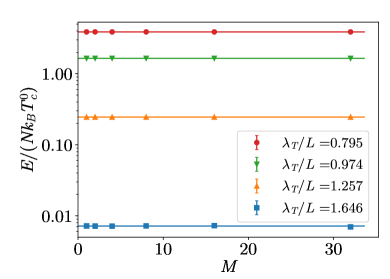
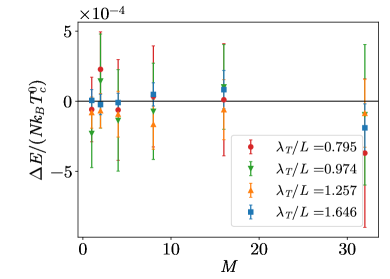
Figure 1: Results for the $N=1$ system at different values of $\lambda_{T}/L$. Left: Internal energy $E$, in units of $Nk_{B}T_{c}^{0}$, with $T_{c}^{0}$ being the critical temperature defined in eq. (49). The values obtained at different number of beads $M$ are compared with the exact results (horizontal lines). Right: Differences with the exact values.

II.4.6 Move tail

Similarly, with move tail we redraw the first beads of the worm by selecting a time slice $j_{0}$ and generating a proposal $\bm{\mathrm{r}}_{T}^{\prime}$ for the new tail bead of the worm $\bm{\mathrm{x}}_{i_{T},0}$ according to the distribution

$$\rho_{\mathrm{free}}^{\mathrm{sp}}(\bm{\mathrm{r}}_{T}^{\prime},\bm{\mathrm{r}}_{i_{T},j_{0}},\Delta j\,\delta_{\tau})=(4\pi\lambda\Delta j\,\delta_{\tau})^{-D/2}\exp\left[-\frac{(\bm{\mathrm{r}}_{T}^{\prime}-\bm{\mathrm{r}}_{i_{T},j_{0}})^{2}}{4\lambda\Delta j\,\delta_{\tau}}\right]\,,$$ (42)

where $i_{T}$ is the particle index of the worm’s tail and $\Delta j=M-j_{0}$. We set $\bm{\mathrm{x}}_{i_{T},0}=\bm{\mathrm{r}}_{T}^{\prime}$ and then construct a free path $\bm{\mathrm{r}}_{i_{T},1}^{\prime},\dots,\bm{\mathrm{r}}_{i_{T},j_{0}-1}^{\prime}$ with the staging algorithm. We accept the update with probability

$$A_{T}=\min\left\{1,\exp\left[\sum_{j=j_{0}}^{M-1}\left(U(\bm{\mathrm{R}}_{j},\bm{\mathrm{R}}_{j+1})-U(\bm{\mathrm{R}}_{j}^{\prime},\bm{\mathrm{R}}_{j+1}^{\prime})\right)\right]\right\}\,.$$ (43)

If the coordinate $\bm{\mathrm{r}}_{T}^{\prime}$ falls outside of the fundamental cell, we recenter the tail polymer as discussed above.

III Non-interacting Bose gas

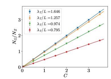
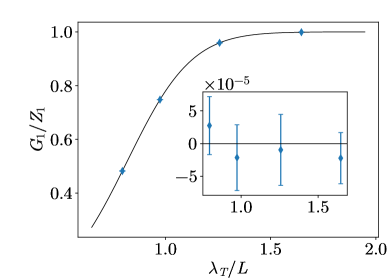
Figure 2: Results for the $N=1$ system at different values of $\lambda_{T}/L$. Left: check of the proportionality in eq. (22), the lines are one-parameter fits. Right: the proportionality coefficients extracted from the fits (diamonds) are compared with the exact value (solid line). Inset: difference between the coefficients and the exact value.

When developing a code, one should have precise benchmarks aimed at validating the various aspects of the algorithm. In this section we start with tests for non-interacting systems, where exact results are known, and we will consider interacting systems in the next section. From now on we specialize to the $D=3$ case. Textbook treatments of the non-interacting Bose gas model usually consider the system in the grand-canonical ensemble and in the thermodynamic limit. However, exact solutions are available also for a fixed number of particles in a box with periodic boundary conditions. In particular, we are interested in the calculation of the internal energy

$$E=-\frac{1}{Z_{N}}\frac{\partial Z_{N}}{\partial\beta}\;.$$ (44)

The partition function $Z_{N}(\beta)$ for $N$ particles at inverse temperature $\beta$ can be calculated using the recursion formula [32, 33]

$$Z_{N}(\beta)=\frac{1}{N}\sum_{k=1}^{N}z(k\beta)Z_{N-k}(\beta)\;,$$ (45)

involving the partition functions of $N-k$ particles at the same inverse temperature $\beta$ with the starting value $Z_{0}(\beta)=1$ and the partition function of a single particle $z(k\beta)$ at the multiple inverse temperature $k\beta$. The latter partition function for our system with periodic boundary conditions is defined as

$$z(\beta)=\sum_{n_{x},n_{y},n_{z}}e^{-\beta\varepsilon(n_{x},n_{y},n_{z})}\;,$$ (46)

where $\varepsilon(n_{x},n_{y},n_{z})$ are the single-particle energies labeled by the integers $n_{x,y,z}=0,\pm 1,\pm 2,\dots$

$$\varepsilon(n_{x},n_{y},n_{z})=\lambda\left(\frac{2\pi}{L}\right)^{2}(n_{x}^{2}+n_{y}^{2}+n_{z}^{2})\;.$$ (47)

The calculation of the internal energy $E$ in Eq. (44) can be carried out recursively from the derivatives with respect to $\beta$ using result (45).

In the following we perform PIMC calculations of the internal energy of $N$ non-interacting bosons at different temperatures and we directly compare the results with the exact value obtained from Eq. (44). First we compare for the case $N=1$, where no swap moves are involved in the PIMC simulation but it provides a stringent benchmark for all the other moves. Then we move to $N=2$ in order to test the correct implementation also of the swap moves. Finally we consider the case $N\gg 1$ and the approach to the thermodynamic limit.

III.1 Benchmarks

We carry out a first non-trivial check on the worm algorithm by considering a single particle in a regime where the thermal wavelength $\lambda_{T}$ is of the order of the side of the box $L$, thus testing the compatibility of the updates (except swap) with the periodic boundary conditions. In fig. 1 we present the results for the internal energy $E$ for different values of the ratio $\lambda_{T}/L$ and compare them with the exact results. We performed the test varying the total number of beads $M$ while keeping unconstrained the simulation parameters controlling the portion of the polymers involved in the moves, namely setting $j_{\mathrm{max}}$ and $j_{\mathrm{max}}^{\mathrm{open}}$ to the maximum value $M$. Since, in the absence of the interaction, the algorithm is exact for any number of beads, we recover the exact result even for $M=1$.

We then turn a closer look to the open/close update, verifying the proportionality between the ratio $N_{G}/N_{Z}$ and the parameter $C$, as expressed in eq. (22). In the left panel of fig. 2 we report the ratios obtained at different values of $C$ together with one-parameter fits. In the right panel, the fitted coefficient is in turn compared with the exact value of $G_{1}/Z_{1}$ given by

$$\frac{G_{1}}{Z_{1}}=\left[\vartheta_{3}\left(0,e^{-\pi\frac{\lambda_{T}^{2}}{L^{2}}}\right)\right]^{-3}\,,$$ (48)

where $\vartheta_{3}(z,q)$ is the theta function with rational characteristic $3$ (see e.g. chapter 16 of ref. [34]). As one can see from the figure, there is perfect agreement between the PIMC points and the expected results, with the inset showing the difference between them.

We now move to the $N=2$ system where the swap update makes its first appearance and we check the results for different values of $\lambda_{T}/L$ and various values of $M$. As before, we used unconstrained parameters $j_{\mathrm{max}}=j_{\mathrm{max}}^{\mathrm{open}}=j_{\mathrm{max}}^{\mathrm{swap}}=M$, allowing updates involving a whole polymer. We report the results in fig. 3, where we show that we recover the exact result for any number of beads used, meaning that the implementation of the swap is fully compatible with periodic boundary conditions.

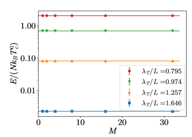
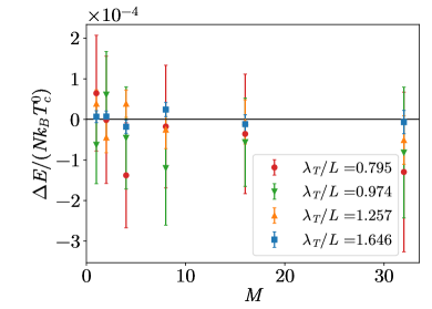
Figure 3: Results for the $N=2$ system at different values of $\lambda_{T}/L$. Left: Internal energy $E$ computed with different number of beads $M$ and compared with the exact results (horizontal lines). As in fig. 1 the energy scale is defined in eq. (49). Right: Differences with the exact values.

The one and two-particle systems provide clean—and to some extent independent—tests for the whole set of updates in the regime where the effect of periodic boundary conditions is the largest. We now show that the exactness of the algorithm is preserved when taking larger and larger numbers of particles. For this purpose we vary $N$ while keeping the temperature $T$ fixed. In fig. 4 we show the results for the internal energy for three values of the temperature, expressed in units of the critical temperature $T_{c}^{0}$ defined as

$$k_{B}T_{c}^{0}=4\pi\lambda\left(\frac{n}{\zeta(3/2)}\right)^{2/3}\;,$$ (49)

where $n=N/V$ is the number density. For every value of $N$ the worm algorithm gives results which are in agreement with the exact values computed from eq. (45) and shown in the left panel of fig. 4 with the dot-dashed lines. Notice that the error bars are of the order of $10^{-4}$ and are completely hidden by the symbols. The horizontal dotted lines represent the value of the internal energy in the thermodynamic limit. In the right panel of fig. 4 we show a linear fit in $1/N$ that extrapolates to the thermodynamic limit the three largest system sizes at $T=0.5T_{c}^{0}$. The gray band covers the $1$-sigma region of the linear fit and perfectly recovers the $N\to\infty$ result shown by the horizontal dotted line.

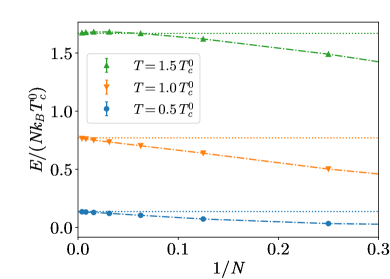
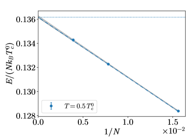
Figure 4: Internal energy $E$ for $N$-particle systems at fixed temperature. Left: Worm algorithm results compared with the exact values at fixed number of particles (dot-dashed lines) and with the exact thermodynamic limit (horizontal dotted lines). Error bars, being of the order of $10^{-4}$, are not visible on this scale and are perfectly compatible with the exact results. Right: Zoom on the $T=0.5T_{c}^{0}$ data, with a linear fit extrapolation to the thermodynamic limit. The gray band covers the one-sigma region of the fit.

IV Hard-spheres Bose gas

In this section we consider interacting systems described by the following microscopic Hamiltonian with two-body interactions

$$H=-\lambda\sum_{i=1}^{N}\nabla_{i}^{2}+\sum_{i<k}v(|\bm{\mathrm{r}}_{i}-\bm{\mathrm{r}}_{k}|)\,,$$ (50)

where $m$ is the mass of the $N$ identical bosons and $\bm{\mathrm{r}}_{i}$ indicates the particle position vector. For pedagogical reasons we use a simple interatomic potential corresponding to a purely repulsive hard core, without any attractive tail to avoid the occurrence of possible cluster bound states. More precisely, we use the hard-sphere (HS) model defined as

$$v(r)=\begin{cases}+\infty&(r<a)\,,\\ 0&(r>a)\,,\end{cases}$$ (51)

in terms of the HS diameter $a$. Besides the degeneracy parameter $n\lambda_{T}^{3}$, only one extra parameter, the gas parameter $na^{3}$, is needed to fully characterize the many-body physics of the model. Equilibrium states of the system correspond either to a gas or to a solid, the latter requiring that the gas parameter be large enough and the temperature small enough [35, 36]. Furthermore, in the limit of a small gas parameter, the HS model fully captures the universal behavior of dilute gases in terms of the $s$-wave scattering length, which coincides with the HS diameter $a$. A careful study of the thermodynamics of the HS model in the dilute regime has been carried out in Ref. [37]. Here, for illustrative reasons, we consider the HS gas at a much higher density $na^{3}=0.1$, which is not so far from the corresponding density of liquid ⁴He and where the issues of convergence with the number of beads are more relevant.

A convenient approximation scheme for the high temperature density matrix entering the PIMC algorithm is the pair-product ansatz [3]

$$\rho(\bm{\mathrm{R}},\bm{\mathrm{R}}^{\prime},\delta_{\tau})=\prod_{i=1}^{N}\rho_{\mathrm{free}}^{\mathrm{sp}}(\bm{\mathrm{r}}_{i},\bm{\mathrm{r}}_{i}^{\prime},\delta_{\tau})\prod_{i<k}\frac{\rho_{rel}(\bm{\mathrm{r}}_{ik},\bm{\mathrm{r}}_{ik}^{\prime},\delta_{\tau})}{\rho_{rel}^{0}(\bm{\mathrm{r}}_{ik},\bm{\mathrm{r}}_{ik}^{\prime},\delta_{\tau})}\;.$$ (52)

In the above equation $\rho_{\mathrm{free}}^{\mathrm{sp}}$ is the single-particle ideal-gas density matrix defined in eq. (19) and $\rho_{rel}$ is the two-body density matrix of the interacting system, which depends on the relative coordinates $\bm{\mathrm{r}}_{ik}=\bm{\mathrm{r}}_{i}-\bm{\mathrm{r}}_{k}$ and $\bm{\mathrm{r}}_{ik}^{\prime}=\bm{\mathrm{r}}_{i}^{\prime}-\bm{\mathrm{r}}_{k}^{\prime}$, divided by the corresponding ideal-gas term

$$\rho_{rel}^{0}(\bm{\mathrm{r}}_{ik},\bm{\mathrm{r}}_{ik}^{\prime},\delta_{\tau})=\left(8\pi\lambda\delta_{\tau}\right)^{-3/2}\exp\left[-\frac{(\bm{\mathrm{r}}_{ik}-\bm{\mathrm{r}}_{ik}^{\prime})^{2}}{8\lambda\delta_{\tau}}\right]\;.$$ (53)

The advantage of the decomposition in eq. (52) is that the two-body density matrix at the inverse temperature $\delta_{\tau}$, $\rho_{rel}(\bm{\mathrm{r}},\bm{\mathrm{r}}^{\prime},\delta_{\tau})$, can be calculated exactly for a given potential $V(r)$, thereby solving by construction the two-body problem. This is the most effective strategy when the system is dilute, but can also be pursued at higher density. For the HS potential a simple and remarkably accurate analytical approximation of the high-energy two-body density matrix is due to Cao and Berne [38]. For $r>a$ and $r^{\prime}>a$, the result is given by

$$\frac{\rho_{rel}(\bm{\mathrm{r}},\bm{\mathrm{r}}^{\prime},\delta_{\tau})}{\rho_{rel}^{0}(\bm{\mathrm{r}},\bm{\mathrm{r}}^{\prime},\delta_{\tau})}=1-\frac{a(r+r^{\prime})-a^{2}}{rr^{\prime}}e^{-[rr^{\prime}+a^{2}-a(r+r^{\prime})](1+\cos\theta)/(4\lambda\delta_{\tau})}\;,$$ (54)

where $\theta$ is the angle between the directions of $\bf{r}$ and $\bf{r}^{\prime}$, while it vanishes when either $r$ or $r^{\prime}$ are smaller than $a$. An important remark concerning the Cao–Berne approximation is that it correctly describes the scattering of hard spheres at high energy (small $\delta_{\tau}$), and it exactly accounts for the $s$-wave term in the partial wave expansion, which is the dominant contribution at low energy. Within the Cao–Berne approximation, the interaction energy of hard spheres evaluated at two subsequent beads $j$ and $j+1$ can finally be written as (setting $\bm{\mathrm{R}}=\bm{\mathrm{R}}_{j}$ and $\bm{\mathrm{R}}^{\prime}=\bm{\mathrm{R}}_{j+1}$)

$$U(\bm{\mathrm{R}},\bm{\mathrm{R}}^{\prime})=-\sum_{i<k}\log\bigg{(}\dfrac{\rho_{rel}(\bm{\mathrm{r}}_{ik},\bm{\mathrm{r}}_{ik}^{\prime},\delta_{\tau})}{\rho_{rel}^{0}(\bm{\mathrm{r}}_{ik},\bm{\mathrm{r}}_{ik}^{\prime},\delta_{\tau})}\bigg{)}\,.$$ (55)

In the following subsections we investigate the convergence with the number of beads for different number of particles and different temperatures at the density $na^{3}=0.1$. Finally we investigate the approach to the thermodynamic limit for increasing values of $N$ at a specific temperature.

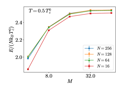
Figure 5: Internal energy $E$ for a system of hard-spheres bosons at the density $na^{3}=0.1$, shown as a function of the number of beads used in the simulation. The energy is computed using the virial estimator reported in appendix.

IV.1 Benchmarks

The presence of the hard-sphere potential, approximated by the product of Cao–Berne density matrices brings a dependence on the number of beads that is detectable when the gas parameter is large enough. In fig. 5 we show such dependence in a system at density $na^{3}=0.1$ for two values of the temperature, $T=T_{c}^{0}$ and $T=0.5T_{c}^{0}$. As one can see, the value of the energy saturates at large number of beads, regardless of the system size controlled by the total number of particles $N$. This can be interpreted recalling that the Cao–Berne density matrix computes exactly the scattering at high energy, requiring the thermal wavelength associated with the imaginary time step $\delta_{\tau}$ to be small compared to the interaction range $a$, i.e.

$$\sqrt{\frac{4\pi\lambda\beta}{M}}\ll a\,.$$ (56)

On the contrary, in the limit of dilute systems the Cao–Berne approximation becomes exact and even a small number of beads (even $8$ or $16$) is sufficient to get precise results [37]. Finally, in fig. 6 we show how the points at $M=64$ from fig. 5 extrapolate to the thermodynamic limit for the two temperatures. In the left and right panels of fig. 6 the dotted lines represent the linear fit to the data, with the gray bands covering the one-sigma region. As expected, the system at the critical temperature $T_{c}^{0}$ suffers from much larger finite size effects, compared with the system at temperature $T=0.5T_{c}^{0}$.

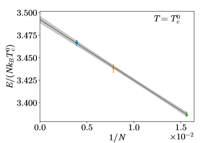
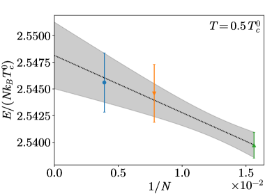
Figure 6: Extrapolation of the internal energy $E$ to the thermodynamic limit using the points at $M=64$ from fig. 5. We have omitted the system size $N=16$ because it is too small to be used in a linear extrapolation in $1/N$. Symbols follow the legend in fig. 5.

V Conclusions

We described an algorithm to perform unbiased PIMC simulations for Bose systems in the canonical ensemble with periodic boundary conditions. The formalism for path-integrals suitable for periodic systems has been developed, and the technical details required for a correct implementation of the PIMC algorithm have been discussed in a pedagogical manner. The formalism can be similarly applied to the simulation of systems in the grand-canonical ensemble. Benchmark results have been presented for non-interacting Bose gases, for which the energy can be exactly computed for any particle number. Many-body systems with hard-sphere interactions have been addressed as well, and the convergence to the continuous imaginary-time limit and to the infinite system-size limit have been analyzed. The PIMC algorithm we presented provides unbiased results for non-interacting Bose gases with periodic boundary conditions for any number of imaginary-time slices, meaning that, e.g., non-interacting particles can be exactly simulated even setting $M=1$. Furthermore, all Monte Carlo updates can be performed without limitations on the length of the paths that are involved in the update, even in regimes where the thermal wavelength is comparable to the size of the fundamental cell. This is in contrast to previous implementations of the worm algorithm [8], for which, even for non-interacting systems, unbiased results are obtained only for a sufficiently large number of imaginary-time slices. Furthermore, those implementations become ambiguous when the thermal wavelength starts to be comparable to the size of the fundamental cell, possibly leading to biased results unless the length of the paths that are involved in some updates is constrained. For interacting systems, also the PIMC algorithm presented here requires a sufficient number of imaginary-time slices, so that the high-temperature approximation for the density matrix (in our case, the pair product approximation) becomes essentially exact. However, there is no constraint on the length of the paths involved in any updates. It is worth emphasizing that the original implementation of the worm algorithm provides unbiased results, even without constraints in the Monte Carlo updates, if the size of the fundamental periodic cell is much larger than the thermal wavelength. While such a system size is feasible for high and for moderately low temperatures, it becomes impractical close to the zero temperature limit. When the thermal wavelength starts to be comparable to the size of the fundamental periodic cell, stringent constraints in some Monte Carlo updates have to be imposed in order to avoid ambiguities due to the choice of periodic images. These constraints strongly reduce the acceptance rates, leading to excessively long autocorrelation times and, therefore, to inefficient simulations. For these reasons, we expect the algorithm presented here to allow extending the scope of the PIMC simulations, providing a better access to the intriguing quantum phenomena occurring in the low temperature limit. Furthermore, the possibility to perform exact benchmarks for small system sizes will help novel practitioners in correctly implementing unbiased PIMC codes.

APPENDIX

In this appendix we report the expressions needed to compute the internal energy $E$ and pressure $P$ in a PIMC simulation, presenting two Monte Carlo estimators for each of them.

.1 Energy

The internal energy $E$ can be computed in the diagonal sector as

$$E=-\frac{1}{Z_{N}}\frac{dZ_{N}}{d\beta}\,.$$ (57)

Using the PIMC representation of $Z_{N}$ in eq. (14) and working out the derivative, we obtain the thermodynamic estimator

$$\frac{E_{\mathrm{th}}}{N}=\left<\frac{D}{2\delta_{\tau}}-\frac{1}{4\lambda\delta_{\tau}^{2}NM}\sum_{j=0}^{M-1}\left(\bm{\mathrm{R}}_{j}-\bm{\mathrm{R}}_{j+1}\right)^{2}+\frac{1}{NM}\sum_{j=0}^{M-1}\frac{\partial U\left(\bm{\mathrm{R}}_{j},\bm{\mathrm{R}}_{j+1}\right)}{\partial\delta_{\tau}}\right>,$$ (58)

where the average is taken on the configurations sampled in the $Z$-sectors. In addition, the above quantity can be calculated in PIMC simulations using the so called virial estimator [3], which usually suffers from smaller statistical fluctuations. Different expressions can be derived, we report here the version we have implemented in our code

$$\frac{E_{\mathrm{vir}}}{N}=\Bigg{<}\frac{D}{2\beta}+\frac{\left(\bm{\mathrm{R}}_{M-1}-\bm{\mathrm{R}}_{M}\right)\cdot\left(\bm{\mathrm{R}}_{M}-\bm{\mathrm{R}}_{0}\right)}{4\lambda\delta_{\tau}^{2}NM}+\frac{1}{2\beta N}\sum_{j=1}^{M-1}\left(\bm{\mathrm{R}}_{j}-\bm{\mathrm{R}}_{0}\right)\cdot\frac{\partial}{\partial\bm{\mathrm{R}}_{j}}\left[U\left(\bm{\mathrm{R}}_{j-1},\bm{\mathrm{R}}_{j}\right)+U\left(\bm{\mathrm{R}}_{j},\bm{\mathrm{R}}_{j+1}\right)\right]\\ +\frac{1}{NM}\sum_{j=0}^{M-1}\frac{\partial U\left(\bm{\mathrm{R}}_{j},\bm{\mathrm{R}}_{j+1}\right)}{\partial\tau}\Bigg{>}.$$ (59)

.2 Pressure

Although we have not presented any results for the pressure, we report for completeness the expression for its two estimators. The pressure is defined as

$$P=\frac{1}{\beta Z_{N}}\frac{dZ_{N}}{dV}\;.$$ (60)

To calculate the derivative of the partition function with respect to the volume $V$, we use the identity $Vd\bm{\mathrm{R}}_{j}/dV=\bm{\mathrm{R}}_{j}/D$ and apply the chain rule for every $j$. The thermodynamic estimator reads

$$\frac{P_{\mathrm{th}}}{n}=\Bigg{<}\frac{1}{\delta_{\tau}}-\frac{1}{2\lambda\delta_{\tau}^{2}NMD}\sum_{j=0}^{M-1}\left(\bm{\mathrm{R}}_{j}-\bm{\mathrm{R}}_{j+1}\right)^{2}-\frac{V}{\beta N}\sum_{j=0}^{M-1}\frac{\partial U(\bm{\mathrm{R}}_{j},\bm{\mathrm{R}}_{j+1})}{\partial V}\Bigg{>}\,.$$ (61)

Notice that we have not used the chain rule on the last term because, depending on the interatomic potential and on the adopted approximation for the density matrix, it is sometimes easier to directly compute the derivative of the interaction term (e.g. the expression in eq. (55)) with respect to the volume, obtaining an expression without ambiguities due to periodic boundary conditions. The virial estimator can instead be computed as

$$\frac{P_{\mathrm{vir}}}{n}=\Bigg{<}\frac{1}{\beta}+\frac{\left(\bm{\mathrm{R}}_{M-1}-\bm{\mathrm{R}}_{M}\right)\cdot\left(\bm{\mathrm{R}}_{M}-\bm{\mathrm{R}}_{0}\right)}{2\lambda\delta_{\tau}^{2}NMD}+\frac{1}{\beta ND}\sum_{j=1}^{M-1}\left(\bm{\mathrm{R}}_{j}-\bm{\mathrm{R}}_{0}\right)\cdot\frac{\partial}{\partial\bm{\mathrm{R}}_{j}}\left[U\left(\bm{\mathrm{R}}_{j-1},\bm{\mathrm{R}}_{j}\right)+U\left(\bm{\mathrm{R}}_{j},\bm{\mathrm{R}}_{j+1}\right)\right]\\ -\frac{V}{\beta N}\sum_{j=0}^{M-1}\frac{\partial U(\bm{\mathrm{R}}_{j},\bm{\mathrm{R}}_{j+1})}{\partial V}\Bigg{>}.$$ (62)

References

- Pollock and Ceperley [1984] E. L. Pollock and D. M. Ceperley, Simulation of quantum many-body systems by path-integral methods, Physical Review B 30, 2555 (1984).
- Ceperley and Pollock [1986] D. M. Ceperley and E. L. Pollock, Path-integral computation of the low-temperature properties of liquid , Phys. Rev. Lett. 56, 351 (1986).
- Ceperley [1995] D. M. Ceperley, Path integrals in the theory of condensed helium, Rev. Mod. Phys. 67, 279 (1995).
- Pollock and Ceperley [1987] E. L. Pollock and D. M. Ceperley, Path-integral computation of superfluid densities, Physical Review B 36, 8343 (1987).
- Boninsegni [2005] M. Boninsegni, Permutation Sampling in Path Integral Monte Carlo, Journal of Low Temperature Physics 141, 27–46 (2005).
- Prokof’ev et al. [1998] N. Prokof’ev, B. Svistunov, and I. S. Tupitsyn, “Worm” algorithm in quantum Monte Carlo simulations, Physics Letters A 238, 253 (1998).
- Prokof’ev and Svistunov [2001] N. Prokof’ev and B. Svistunov, Worm algorithms for classical statistical models, Physical Review Letters 87, 160601 (2001).
- Boninsegni et al. [2006a] M. Boninsegni, N. Prokof’ev, and B. Svistunov, Worm algorithm and diagrammatic Monte Carlo: A new approach to continuous-space path integral Monte Carlo simulations, Physical Review E 74, 036701 (2006a).
- Boninsegni et al. [2006b] M. Boninsegni, N. Prokof’ev, and B. Svistunov, Worm algorithm for continuous-space path integral Monte Carlo simulations, Physical Review Letters 96, 070601 (2006b).
- Cinti et al. [2017] F. Cinti, A. Cappellaro, L. Salasnich, and T. Macrì, Superfluid Filaments of Dipolar Bosons in Free Space, Phys. Rev. Lett. 119, 215302 (2017).
- Cinti, F. and Wang, D.-W. and Boninsegni, M. [2017] Cinti, F. and Wang, D.-W. and Boninsegni, M., Phases of dipolar bosons in a bilayer geometry, Physical Review A 95, 10.1103/PhysRevA.95.023622 (2017).
- Bombín et al. [2019] R. Bombín, F. Mazzanti, and J. Boronat, Berezinskii-Kosterlitz-Thouless transition in two-dimensional dipolar stripes, Phys. Rev. A 100, 063614 (2019).
- Cinti et al. [2010] F. Cinti, P. Jain, M. Boninsegni, A. Micheli, P. Zoller, and G. Pupillo, Supersolid Droplet Crystal in a Dipole-Blockaded Gas, Phys. Rev. Lett. 105, 135301 (2010).
- Saccani et al. [2011] S. Saccani, S. Moroni, and M. Boninsegni, Phase diagram of soft-core bosons in two dimensions, Phys. Rev. B 83, 092506 (2011).
- Carleo et al. [2013] G. Carleo, G. Boéris, M. Holzmann, and L. Sanchez-Palencia, Universal Superfluid Transition and Transport Properties of Two-Dimensional Dirty Bosons, Phys. Rev. Lett. 111, 050406 (2013).
- Cinti et al. [2014] F. Cinti, T. Macrì, W. Lechner, G. Pupillo, and T. Pohl, Defect-induced supersolidity with soft-core bosons, Nature Communications 5, 3235 (2014).
- Pascual and Boronat [2021] G. Pascual and J. Boronat, Quasiparticle Nature of the Bose Polaron at Finite Temperature, Phys. Rev. Lett. 127, 205301 (2021).
- Boninsegni et al. [2006c] M. Boninsegni, N. Prokof’ev, and B. Svistunov, Superglass Phase of , Phys. Rev. Lett. 96, 105301 (2006c).
- Boninsegni et al. [2006d] M. Boninsegni, A. B. Kuklov, L. Pollet, N. V. Prokof’ev, B. V. Svistunov, and M. Troyer, Fate of Vacancy-Induced Supersolidity in , Phys. Rev. Lett. 97, 080401 (2006d).
- Corboz et al. [2008] P. Corboz, M. Boninsegni, L. Pollet, and M. Troyer, Phase diagram of adsorbed on graphite, Phys. Rev. B 78, 245414 (2008).
- Boninsegni [2009] M. Boninsegni, Quantum statistics and the momentum distribution of liquid parahydrogen, Phys. Rev. B 79, 174203 (2009).
- Rota and Boronat [2011] R. Rota and J. Boronat, Path Integral Monte Carlo Calculation of Momentum Distribution in Solid 4He, Journal of Low Temperature Physics 162, 146 (2011).
- Osychenko et al. [2012] O. N. Osychenko, R. Rota, and J. Boronat, Superfluidity of metastable glassy bulk para-hydrogen at low temperature, Phys. Rev. B 85, 224513 (2012).
- Ferré and Boronat [2016] G. Ferré and J. Boronat, Dynamic structure factor of liquid across the normal-superfluid transition, Phys. Rev. B 93, 104510 (2016).
- Metropolis et al. [1953] N. Metropolis, A. W. Rosenbluth, M. N. Rosenbluth, A. H. Teller, and E. Teller, Equation of state calculations by fast computing machines, The journal of chemical physics 21, 1087 (1953).
- Hastings [1970] W. K. Hastings, Monte Carlo sampling methods using Markov chains and their applications, Biometrika 57, 97 (1970).
- Trotter [1959] H. F. Trotter, On the product of semi-groups of operators, Proceedings of the American Mathematical Society 10, 545 (1959).
- Sprik et al. [1985] M. Sprik, M. L. Klein, and D. Chandler, Staging: A sampling technique for the Monte Carlo evaluation of path integrals, Physical Review B 31, 4234 (1985).
- Sakkos et al. [2009] K. Sakkos, J. Casulleras, and J. Boronat, High order Chin actions in path integral Monte Carlo, The Journal of Chemical Physics 130, 204109 (2009).
- Prokof’ev et al. [1998] N. V. Prokof’ev, B. V. Svistunov, and I. S. Tupitsyn, Exact, complete, and universal continuous-time worldline Monte Carlo approach to the statistics of discrete quantum systems, Journal of Experimental and Theoretical Physics 87, 310 (1998).
- Lévy [1940] P. Lévy, Sur certains processus stochastiques homogènes, Compositio mathematica 7, 283 (1940).
- Borrmann, Peter and Franke, Gert [1993] Borrmann, Peter and Franke, Gert, Recursion formulas for quantum statistical partition functions, The Journal of Chemical Physics 98, 2484 (1993).
- Krauth, Werner [2006] Krauth, Werner, Statistical Mechanics Algorithms and Computations (Oxford University Press, Oxford, 2006).
- Abramowitz and Stegun [1965] M. Abramowitz and I. A. Stegun, eds., Handbook of mathematical functions, Dover Books on Mathematics (Dover Publications, Mineola, NY, 1965).
- Hansen et al. [1971] J.-P. Hansen, D. Levesque, and D. Schiff, Fluid-Solid Phase Transition of a Hard-Sphere Bose System, Phys. Rev. A 3, 776 (1971).
- Kalos et al. [1974] M. H. Kalos, D. Levesque, and L. Verlet, Helium at zero temperature with hard-sphere and other forces, Phys. Rev. A 9, 2178 (1974).
- Spada et al. [2022] G. Spada, S. Pilati, and S. Giorgini, Thermodynamics of a dilute Bose gas: A path-integral Monte Carlo study, Phys. Rev. A 105, 013325 (2022).
- Cao and Berne [1992] J. Cao and B. J. Berne, A new quantum propagator for hard sphere and cavity systems, J. Chem. Phys. 97, 2382 (1992).