Abstract. We develop a mixtures-of-experts (ME) approach to the multiclass classification where the predictors are univariate functions. It consists of a ME model in which both the gating network and the experts network are constructed upon multinomial logistic activation functions with functional inputs. We perform a regularized maximum likelihood estimation in which the coefficient functions enjoy interpretable sparsity constraints on targeted derivatives. We develop an EM-Lasso like algorithm to compute the regularized MLE and evaluate the proposed approach on simulated and real data.

Keywords. Mixtures of experts, Functional predictors, EM algorithm, Sparsity

1 Introduction

Introduced in Jacobs et al., (1991), a mixtures of experts (ME) model can be defined as

$$\textstyle f(y|x)=\sum_{k=1}^{K}\text{Gate}_{k}(x)\,\text{Expert}_{k}(y|x),$$ (1)

in which $f(y|x)$, the distribution of the response $y$ given the covariate $x$, is modeled as a mixture distribution with covariate-dependent mixing proportions $\text{Gate}_{k}(x)$, referred to as gating functions, and conditional mixture components $\text{Expert}_{k}(y|x)$, referred to as experts functions, $K$ being the number of experts. Some ME studies that may be mentioned here include ME for time series prediction (Zeevi et al.,, 1996; Yümlü et al.,, 2003), segmentation (Chamroukhi et al.,, 2013, 2009), ME for classification of gender and pose of human faces (Gutta et al.,, 2000), for social network data (Gormley and Murphy,, 2010), among others. For an overview of practical and theoretical aspects of ME modeling, the reader is referred to Nguyen and Chamroukhi, (2018). The study of ME for functional data analysis (FDA) (Ramsay and Silverman,, 2005), is still however less investigated. In a recent study, we introduced in Chamroukhi et al., (2022) a functional ME (FME) framework for regression and clustering of observed pairs of scalar responses and univariate functional inputs.

2 Functional Mixture-of-Experts for classification

In this paper, we extend the FME framework for multiclass classification, derive adapted EM-like algorithms to obtain sparse and interpretable fit of the gating and experts network coefficients functions. Let $\{X_{i}(t),t\in\mathcal{T};Y_{i}\}_{i=1}^{n}$, be a sample of $n$ i.i.d. data pairs where $Y_{i}\in\{1,\ldots,G\}$ is the class label of a functional predictor $X_{i}(\cdot)$, $G$ being the number of classes. In this case of functional inputs, a natural choice to model the conditional distribution $\text{Expert}_{k}(y|x)=\mathbb{P}(Y=y|X_{i}(\cdot))$ in (1) is to use the functional multinomial logistic regression modeling, see e.g., Müller et al., (2005); James, (2002), that is

$$P(y_{i}|X_{i}(\cdot);\bm{\beta}_{k})=\prod_{g=1}^{G}\left[\frac{\exp\left\{\beta_{kg,0}+\int_{\mathcal{T}}X_{i}(t)\beta_{kg}(t)dt\right\}}{1+\sum_{g^{\prime}=1}^{G-1}\exp\left\{\beta_{kg^{\prime},0}+\int_{\mathcal{T}}X_{i}(t)\beta_{kg^{\prime}}(t)dt\right\}}\right]^{y_{ig}},$$ (2)

whre $\bm{\beta}_{k}$ represents the set of coefficient functions $\{\beta_{kg}(t),t\in\mathcal{T}\}$ and intercepts $\{\beta_{k,0}\}$ for $k\in[K]=\{1,\ldots,K\}$ and $g\in[G]$, and $y_{ig}=\mathbb{I}_{\{y_{i}=g\}}$. Similarly, a typical choice for the functional gating network $\text{Gate}_{k}(x)=\mathbb{P}(Z=k,X(\cdot))$ in (1), where $Z\in[K]$ is a hidden within-class clustering label, acting as weights for potential clusters $\{k\}$ in the heterogeneous functional inputs $X(\cdot)$ and which we denote as $\pi_{k}(X(\cdot))$, is to use a functional softmax function defined by

$$\pi_{k}(X_{i}(\cdot);\bm{\alpha})=\frac{\exp\{\alpha_{k,0}+\int_{\mathcal{T}}X_{i}(t)\alpha_{k}(t)dt\}}{1+\sum_{k^{\prime}=1}^{K-1}\exp\{\alpha_{k^{\prime},0}+\int_{\mathcal{T}}X_{i}(t)\alpha_{k^{\prime}}(t)dt\}},$$ (3)

with $\bm{\alpha}$ is composed of the set of coefficient functions $\{\alpha_{k}(t),t\in\mathcal{T}\}$ and intercepts $\{\alpha_{k,0}\}$ for $k\in[K]$. Then, from (2) and (3) given $X_{i}(\cdot)$, the probability that $Y_{i}=y_{i}$, can be modeled by the following $K$-component FME model for classification

$$P(y_{i}|X_{i}(\cdot);\bm{\psi})=\sum_{k=1}^{K}\pi_{k}(X_{i}(\cdot);\bm{\alpha})P(y_{i}|X_{i}(\cdot);\bm{\beta}_{k}),\quad\bm{\psi}=(\bm{\alpha},\bm{\beta}_{1},\ldots,\bm{\beta}_{K}).$$ (4)

2.1 Smooth functional representation

In practice, $X_{i}(\cdot)$ is observed at a finite but large number of points on $\mathcal{T}\subset\mathbb{R}$. In the perspective of parameter estimation, this results in estimating a very large number of coefficients $\beta$ and $\alpha$. In order to handle this high-dimensional problem, we consider a usual approach that projects the predictors and coefficient functions onto a family of reduced number of basis functions. Let $\bm{b}_{r}(t)=\left[b_{1}(t),\ldots,b_{r}(t)\right]^{\top}$ be a $r$-dimensional basis (B-spline, Wavelet, …). Then, with $r,p,q\in\mathbb{N}$ sufficiently large, one can approximate $X_{i}(\cdot)$, $\alpha_{k}(\cdot)$ and $\beta_{kg}(\cdot)$ respectively by

$$X_{i}(t)=\bm{x}_{i}^{\top}\bm{b}_{r}(t),\quad\alpha_{k}(t)=\bm{\zeta}_{k}^{\top}\bm{b}_{p}(t),\quad\beta_{kg}(t)=\bm{\eta}_{kg}^{\top}\bm{b}_{q}(t).$$ (5)

Here, $\bm{x}_{i}=(x_{i1},\ldots,x_{ir})^{\top}$, with $x_{ij}=\int_{\mathcal{T}}X_{i}(t)b_{j}(t)dt$ for $j\in[r]$, is the vector of coefficients of $X_{i}(\cdot)$ in the basis $\bm{b}_{r}(t)$, $\bm{\zeta}_{k}=(\zeta_{k,1},\ldots,\zeta_{k,p})^{\top}$, and $\bm{\eta}_{kg}=(\eta_{kg,1},\ldots,\eta_{kg,q})^{\top}$ are the unknown coefficient vectors associated with the gating coefficient function $\alpha_{k}(\cdot)$ and the expert coefficient function $\beta_{kg}(\cdot)$ in the corresponding basis. In our case, we used B-spline bases. Using the approximation of $X_{i}(\cdot)$ and $\alpha_{k}(\cdot)$ in (5), the functional softmax gating network (3) can be represented by

$$\pi_{k}(\mathbf{r}_{i};\bm{\xi})=\frac{\exp\{\alpha_{k,0}+\mathbf{r}_{i}^{\top}\bm{\zeta}_{k}\}}{1+\sum_{k^{\prime}=1}^{K-1}\exp\{\alpha_{k^{\prime},0}+\mathbf{r}_{i}^{\top}\bm{\zeta}_{k^{\prime}}\}},$$ (6)

where $\mathbf{r}_{i}=\left[\int_{\mathcal{T}}\bm{b}_{r}(t)\bm{b}_{p}(t)^{\top}dt\right]^{\top}\bm{x}_{i}$ is the design vector associated with the gating network and $\bm{\xi}=((\alpha_{1,0},\bm{\zeta}_{1}^{\top}),\ldots,(\alpha_{K-1,0},\bm{\zeta}_{K-1}^{\top}))\allowbreak\in\mathbb{R}^{(p+1)(K-1)}$ is the unknown parameter vector of the gating network, to be estimated. In the same manner, using the approximations of $X_{i}(\cdot)$ and $\beta_{kg}(\cdot)$ in (5), the expert conditional distribution (2) can be represented by

$$\textstyle P(y_{i}|\mathbf{x}_{i};\bm{\theta}_{k})=\prod_{g=1}^{G}\left[\frac{\exp\left\{\beta_{kg,0}+\mathbf{x}_{i}^{\top}\bm{\eta}_{kg}\right\}}{1+\sum_{g^{\prime}=1}^{G-1}\exp\left\{\beta_{kg^{\prime},0}+\mathbf{x}_{i}^{\top}\bm{\eta}_{kg^{\prime}}\right\}}\right]^{y_{ig}},$$ (7)

where $\mathbf{x}_{i}=\left[\int_{\mathcal{T}}\bm{b}_{r}(t)\bm{b}_{q}(t)^{\top}dt\right]^{\top}\bm{x}_{i}$ is the design vector associated with the expert network, and $\bm{\theta}_{k}=(\bm{\theta}_{k1}^{\top},\ldots,\bm{\theta}_{k,G-1}^{\top})^{\top}$, with $\bm{\theta}_{kg}=(\beta_{kg,0},\bm{\eta}_{kg}^{\top})^{\top}\in\mathbb{R}^{q+1}$ for $g\in[G-1]$, is the unknown parameter vector to be estimated of the expert distribution $k$. Finally, combining (6) and (7), the conditional distribution $P(y_{i}|X_{i}(\cdot);\bm{\psi})$ in (4) can be rewritten as

$$P(y_{i}|X_{i}(\cdot);\bm{\varPsi})=\sum_{k=1}^{K}\pi_{k}(\mathbf{r}_{i};\bm{\xi})P(y_{i}|\mathbf{x}_{i};\bm{\theta}_{k}),$$

where $\bm{\varPsi}=(\bm{\xi}^{\top},\bm{\theta}_{1}^{\top},\ldots,\bm{\theta}_{K}^{\top})^{\top}$ is the unknown parameter vector of the model.

Parameter estimation: A maximum likelihood estimate (MLE) $\widehat{\bm{\varPsi}}$ of $\bm{\varPsi}$ can be obtained by using the EM algorithm for ME model for classification with vector data as in Chen et al., (1999). We will refer to this approach as FME-EM. To encourage sparsity in the model parameters $\bm{\varPsi}$, one can perform penalized MLE by using the EM-Lasso algorithm as in Huynh and Chamroukhi, (2019). We refer to this approach as FME-EM-Lasso.

2.2 An interpretable sparse estimation of FME for classification

Although fitting the FME model via EM-Lasso can accommodate sparsity in the parameters, it unfortunately does not ensure the reconstructed coefficient functions $\widehat{\alpha}_{k}(\cdot)$ and $\widehat{\beta}_{kg}(\cdot)$ are sparse and enjoy easy interpretable sparsity. To obtain interpretable and sparse fits for the coefficient functions, we simultaneously estimate the model parameters while constraining some targeted derivatives of the coefficient functions to be zero (Chamroukhi et al.,, 2022). The construction of the interpretable FME model which we will fit with an adapted EM algorithm, is as follows. First, in order to calculate the derivative of the gating coefficient functions $\alpha_{k}(\cdot)$, let $\mathbf{A}_{p}$ be the matrix of approximate $d_{1}$th and $d_{2}$th derivative of $\bm{b}_{p}(t)$, defined as in James et al., (2009); Chamroukhi et al., (2022) by

$$\mathbf{A}_{p} = [\mathbf{A}_{p}^{[d_{1}]}\mathbf{A}_{p}^{[d_{2}]}]^{\top}=\left[D^{d_{1}}\bm{b}_{p}(t_{1}),\ldots,D^{d_{1}}\bm{b}_{p}(t_{p}),D^{d_{2}}\bm{b}_{p}(t_{1}),\ldots,D^{d_{2}}\bm{b}_{p}(t_{p})\right]^{\top},$$

where $D^{d}$ is the $d$th finite difference operator. Here $\mathbf{A}_{p}^{[d_{j}]}$ is a square invertible matrix and $\mathbf{A}_{p}\in\mathbb{R}^{2p\times p}$. Similarly, to calculate the derivatives of the expert coefficient functions $\beta_{kg}(\cdot)$, let $\mathbf{A}_{q}=[\mathbf{A}_{q}^{[d_{1}]}\mathbf{A}_{q}^{[d_{2}]}]^{\top}\in\mathbb{R}^{2q\times q}$ be the corresponding matrix defined for the $\bm{b}_{q}(t)$’s. Now, if we define $\bm{\omega}_{k}=\mathbf{A}_{p}\bm{\zeta}_{k}$ and denote $\bm{\omega}_{k}=({\bm{\omega}^{[d_{1}]}_{k}}^{\top},{\bm{\omega}^{[d_{2}]}_{k}}^{\top})^{\top}$, then $\bm{\omega}^{[d_{1}]}_{k}$ and $\bm{\omega}^{[d_{2}]}_{k}$ provide approximations to the $d_{1}$ and the $d_{2}$ derivatives of the coefficient function $\alpha_{k}(\cdot)$, respectively, which we denote as $\alpha_{k}^{(d_{1})}(\cdot)$ and $\alpha_{k}^{(d_{2})}(\cdot)$. Therefore, enforcing sparsity in $\bm{\omega}_{k}$ will constrain $\alpha_{k}^{(d_{1})}(\cdot)$ and $\alpha_{k}^{(d_{2})}(\cdot)$ to be zero at most of time points. Similarly, if we define $\bm{\gamma}_{kg}=\mathbf{A}_{q}\bm{\zeta}_{k}$ and denote by $\bm{\gamma}_{kg}=({\bm{\gamma}^{[d_{1}]}_{kg}}^{\top},{\bm{\gamma}^{[d_{2}]}_{kg}}^{\top})^{\top}$, then we can derive the same regularization for the coefficient functions $\beta_{kg}(\cdot)$. From the definitions of $\bm{\omega}_{k}$ and $\bm{\gamma}_{kg}$ we can easily get the following relations:

$$\bm{\zeta}_{k} ={\mathbf{A}_{p}^{[d_{1}]}}^{-1}\bm{\omega}_{k}^{[d_{1}]}\text{ and }\bm{\omega}_{k}^{[d_{2}]}=\mathbf{A}_{p}^{[d_{2}]}{\mathbf{A}_{p}^{[d_{1}]}}^{-1}\bm{\omega}_{k}^{[d_{1}]}$$ (8a)

$$\bm{\eta}_{kg} ={\mathbf{A}_{q}^{[d_{1}]}}^{-1}\bm{\gamma}_{kg}^{[d_{1}]}\text{ and }\bm{\gamma}_{kg}^{[d_{2}]}=\mathbf{A}_{q}^{[d_{2}]}{\mathbf{A}_{q}^{[d_{1}]}}^{-1}\bm{\gamma}_{kg}^{[d_{1}]}.$$ (8b)

Plugging the relation (8a) into (6) one gets the following new representation for $\pi_{k}(\mathbf{r}_{i};\bm{\xi})$

$$\textstyle\pi_{k}(\mathbf{s}_{i};\mathbf{w})=\frac{\exp{\{\alpha_{k,0}+{\mathbf{s}_{i}^{\top}\bm{\omega}_{k}^{[d_{1}]}}\}}}{1+\sum_{k^{\prime}=1}^{K-1}\exp{\{\alpha_{k^{\prime},0}+{\mathbf{s}_{i}^{\top}\bm{\omega}^{[d_{1}]}_{k^{\prime}}}\}}},$$ (9)

where $\mathbf{s}_{i}=({\mathbf{A}^{[d_{1}]}_{p}}^{-1})^{\top}\mathbf{r}_{i}$ is now the new design vector and $\mathbf{w}=(\alpha_{1,0},{\bm{\omega}^{[d_{1}]}_{1}}^{\top},\ldots,\alpha_{K-1,0},{\bm{\omega}^{[d_{1}]}_{K-1}}^{\top})^{\top}$, with $(\alpha_{K,0},{\bm{\omega}^{[d_{1}]}_{K}}^{\top})^{\top}$ a null vector, is the unknown parameter vector of the gating network. Similarly, plugging (8b) into (7) one obtains the new representation for $P(y_{i}|\mathbf{x}_{i};\bm{\theta}_{k})$:

$$\textstyle P(y_{i}|\mathbf{v}_{i};\bm{\Gamma}_{k})=\prod_{g=1}^{G}\left[\frac{\exp\left\{\beta_{kg,0}+{\mathbf{v}_{i}^{\top}\bm{\gamma}_{kg}^{[d_{1}]}}\right\}}{1+\sum_{g^{\prime}=1}^{G-1}\exp\left\{\beta_{kg^{\prime},0}+{\mathbf{v}_{i}^{\top}\bm{\gamma}_{k^{\prime}g}^{[d_{1}]}}\right\}}\right]^{y_{ig}},$$ (10)

in which, $\mathbf{v}_{i}=({\mathbf{A}^{[d_{1}]}_{q}}^{-1})^{\top}\mathbf{x}_{i}$ is now the new design vector and $\bm{\Gamma}_{k}=(\beta_{kg,0},{\bm{\gamma}_{k^{\prime}g}^{[d_{1}]}}^{\top})^{\top}$ is the unknown parameter vector of the expert network. Finally, gathering the gating network (9) and the expert network (10), the iFME model for classification is given by $P(y_{i}|X_{i}(\cdot);\bm{\Upsilon})=\sum_{k=1}^{K}\pi_{k}(\mathbf{s}_{i};\mathbf{w})P(y_{i}|\mathbf{v}_{i};\bm{\Gamma}_{k}),$ where $\bm{\Upsilon}=(\mathbf{w}^{\top},\bm{\Gamma}_{1}^{\top},\ldots,\bm{\Gamma}_{K}^{\top})^{\top}$ is the unknown parameter vector to be estimated. We perform penalized MLE by penalizing the ML via a Lasso penalization on the derivative coefficients $\bm{\omega}_{k}$’s and $\bm{\gamma}_{kg}$’s of the form Pen${}_{\chi,\lambda}(\bm{\Upsilon})=\chi\sum_{k=1}^{K-1}\|\bm{\omega}_{k}\|_{1}+\lambda\sum_{k=1}^{K}\sum_{g=1}^{G-1}\|\bm{\gamma}_{kg}\|_{1}$, with $\chi$ and $\lambda$ regularization constants. The estimation is performed by using an adaptation to this classification context of the EM algorithm developed in Chamroukhi et al., (2022). The only difference resides in the maximization w.r.t. the expert network parameters $\bm{\Gamma}_{k}$.

3 Numerical results

We conducted experiments by considering a $G=3$-class classification problem with a $K=2$-component FME model. The simulation protocol will be detailed during the presentation due to lack of space here. The classification results obtained with the described algorithms FME-EM, FME-EM-Lasso and iFME-EM, as well as with functional multinomial logistic regression (FMLR), are given in Table 1 and show higher classification performance of the iFME-EM approach.

Model	Correct Classification Rate
	Noise level: $\sigma^{2}_{\delta}=1$	Noise level: $\sigma^{2}_{\delta}=5$
FME-EM	$.8560_{(.0199)}$	$.8474_{(.0196)}$
FME-EM-Lasso	$.9332_{(.0104)}$	$.9178_{(.0142)}$
iFME-EM	$\bm{.9346_{(.0108)}}$	$\bm{.9219_{(.0127)}}$
FMLR	$.7951_{(.0249)}$	$.7922_{(.0270)}$

Table 1: Correct classification rates obtained on testing data. The reported values are averages on 100 samples with standard errors in parentheses.

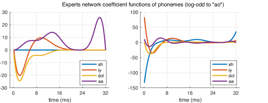
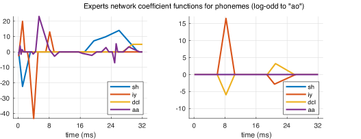
Figure 1: Results of (top) FME-EM-Lasso and (bottom) iFME-EM on phoneme data.

We then applied the two algorithms allowing for sparsity (FME-EM-Lasso and iFME-EM) to the well-known phoneme data (Hastie et al.,, 1995). The data consists of $n=1000$ log-periodogram recordings of length $256$ each, used here as the univariate functional predictors, of five phonemes (the corresponding class labels). The obtained averaged correct classification rate for the two approaches are more than 0.94 in mean. Figure 1 shows the estimated coefficient functions for the expert network $\widehat{\beta}_{kg}(t)$ as functions of sampling time $t$, obtained by FME-EM-Lasso (top) and the iFME-EM (bottom); Here the iFME-EM is fitted with constraints on the zero and the second derivatives of the coefficients functions. The results show clearly sparse and piece-wise-linear gating and experts functions when using the iFME-EM approach.

Acknowledgement:

This research is supported by ANR SMILES ANR-18-CE40-0014.

References

• Chamroukhi et al., (2022) Chamroukhi, F., Pham, T. N., Hoang, V. H., and McLachlan, G. J. (2022). Functional mixtures-of-experts. ArXiv preprint arXiv:2202.02249.
• Chamroukhi et al., (2009) Chamroukhi, F., Samé, A., Govaert, G., and Aknin, P. (2009). Time series modeling by a regression approach based on a latent process. Neural Networks, 22(5-6):593–602.
• Chamroukhi et al., (2013) Chamroukhi, F., Trabelsi, D., Mohammed, S., Oukhellou, L., and Amirat, Y. (2013). Joint segmentation of multivariate time series with hidden process regression for human activity recognition. Neurocomputing, 120:633–644.
• Chen et al., (1999) Chen, K., Xu, L., and Chi, H. (1999). Improved learning algorithms for mixture of experts in multiclass classification. Neural Networks, 12(9):1229–1252.
• Gormley and Murphy, (2010) Gormley, I. C. and Murphy, T. B. (2010). A mixture of experts latent position cluster model for social network data. Statistical Methodology, 7:385–405.
• Gutta et al., (2000) Gutta, S., Huang, J. R., Phillips, P. J., and Wechsler, H. (2000). Mixture of experts for classification of gender, ethnic origin, and pose of human faces. IEEE transactions on neural networks, 11 4:948–60.
• Hastie et al., (1995) Hastie, T., Buja, A., and Tibshirani, R. (1995). Penalized Discriminant Analysis. Annals of Statistics, 23:73–102.
• Huynh and Chamroukhi, (2019) Huynh, T. and Chamroukhi, F. (2019). Estimation and feature selection in mixtures of generalized linear experts models.
• Jacobs et al., (1991) Jacobs, R. A., Jordan, M. I., Nowlan, S. J., and Hinton, G. E. (1991). Adaptive mixtures of local experts. Neural Computation, 3(1):79–87.
• James, (2002) James, G. M. (2002). Generalized linear models with functional predictor variables. Journal of the Royal Statistical Society Series B, 64:411–432.
• James et al., (2009) James, G. M., Wang, J., and Zhu, J. (2009). Functional linear regression that’s interpretable. Annals of Statistics, 37(5A):2083–2108.
• Müller et al., (2005) Müller, H.-G., Stadtmüller, U., et al. (2005). Generalized functional linear models. Annals of Statistics, 33(2):774–805.
• Nguyen and Chamroukhi, (2018) Nguyen, H. D. and Chamroukhi, F. (2018). Practical and theoretical aspects of mixture-of-experts modeling: An overview. Wiley Interdisciplinary Reviews: Data Mining and Knowledge Discovery, pages e1246–n/a.
• Ramsay and Silverman, (2005) Ramsay, J. O. and Silverman, B. W. (2005). Functional Data Analysis. Springer Series in Statistics. Springer.
• Yümlü et al., (2003) Yümlü, M. S., Gürgen, F. S., and Okay, N. (2003). Financial time series prediction using mixture of experts. In ISCIS.
• Zeevi et al., (1996) Zeevi, A. J., Meir, R., and Adler, R. J. (1996). Time series prediction using mixtures of experts. In Proceedings of NIPS’96, page 309–315. MIT Press.