Leveraging Channel Noise for Sampling and Privacy via Quantized Federated Langevin Monte Carlo

Abstract

For engineering applications of artificial intelligence, Bayesian learning holds significant advantages over standard frequentist learning, including the capacity to quantify uncertainty. Langevin Monte Carlo (LMC) is an efficient gradient-based approximate Bayesian learning strategy that aims at producing samples drawn from the posterior distribution of the model parameters. Prior work focused on a distributed implementation of LMC over a multi-access wireless channel via analog modulation. In contrast, this paper proposes quantized federated LMC (FLMC), which integrates one-bit stochastic quantization of the local gradients with channel-driven sampling. Channel-driven sampling leverages channel noise for the purpose of contributing to Monte Carlo sampling, while also serving the role of privacy mechanism. Analog and digital implementations of wireless LMC are compared as a function of differential privacy (DP) requirements, revealing the advantages of the latter at sufficiently high signal-to-noise ratio.

I Introduction

Federated learning (FL) is a distributed learning paradigm whereby multiple devices coordinate to train a target global model, while avoiding the direct sharing of local data with the cloud [1, 2, 3]. Prior work on wireless FL mainly focuses on conventional frequentist learning, which produces point estimates of model parameter vectors by minimizing empirical loss metrics [4, 5, 6, 7, 8, 9]. In many engineering applications characterized by the availability of limited data and by the need to quantify uncertainty, Bayesian learning provides a more effective and principled framework to define the learning problem (see, e.g., [10]). Bayesian learning assigns a probability distribution to the model parameters, rather than collapsing any residual uncertainty in the model parameter space to a single point estimate. In this paper, we focus on the distributed implementation of Bayesian learning in wireless systems within a federated learning setting, with the main goal of leveraging the wireless channel as part of the “compute continuum” between devices and server [11] (see Fig 1).

Scalable Bayesian learning solutions are either based on variational inference, whereby the distribution over the model parameters is optimized by minimizing a free energy metric [12]; or on Monte Carlo (MC) sampling, whereby the distribution over the model parameters is represented by random samples [13]. It was recently pointed out in [14] that MC solutions enable a novel interpretation of the wireless channel as part of the MC sampling process. In particular, reference [14] proposed a Bayesian federated learning protocol based on Langevin MC (LMC), a noise-perturbed gradient-based MC strategy [13], and analog transmission. The paper demonstrated the role of the channel noise as a contributor to the LMC update, as well as a privacy mechanism (see also [15, 16]). In this paper, we devise an alternative strategy that implements LMC in a federated setting via digital modulation under privacy constraints.

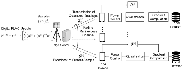
Figure 1: Differentially private quantized federated Bayesian learning system based on LMC.

Federated learning has been widely studied for implementation on wireless channels (see, e.g., [17]). Techniques that leverage the wireless channel for computation include over-the-air computation (AirComp), whereby superposition in non-orthogonal multiple access (NOMA) is used as a means to aggregate information from different sources [18, 8, 19]; channel noise for privacy, which enforces differential privacy (DP) guarantees via power control [20, 16]; and channel noise for sampling, which was introduced above [14]. Also related to this work are DP mechanisms based on stochastic quantization [21].

In this paper, inspired by [7], we study Bayesian federated learning protocols based on the digital transmission of gradients from edge devices to the edge server (see Fig. 1). Like [14], which considered analog transmission, we aim at leveraging channel noise for both channel-driven MC sampling and DP. The main contributions of this paper are as follows.

• Quantized federated LMC (FLMC): We introduce a quantized federated implementation of LMC based on stochastic quantization, binary transmission, and channel-driven sampling;

• Power allocation policy with DP guarantees: We analyze the DP guarantees of LMC, and we design an approach to determine power control parameter to meet the requirements of both MC sampling and DP;

• Experiments: We demonstrate an experimental comparison of digital and analog wireless FLMC implementations under DP constraints.

The remainder of this paper is organized as follows. Section II formulates the system models and definitions. The privacy anaysis and power control design are presented in Section III. Section IV describes numerical results.

II System Model

As shown in Fig. 1, we consider a wireless federated edge learning system comprising an edge server and $K$ edge devices. The devices are connected to the server via a shared wireless channel. Each device $k$ has its own local dataset $\mathcal{D}_{k}$, which includes $N_{k}$ data samples $\mathcal{D}_{k}=\{{\mathbf{d}}_{k,n}\}_{n=1}^{N_{k}}$. The global data set is denoted as $\mathcal{D}=\{\mathcal{D}_{k}\}_{k=1}^{K}$. The devices communicate to the server via a NOMA digital channel with BPSK modulation as in [9]. Unlike [9], which focuses on conventional frequentist learning, here the goal is to carry out Bayesian learning by approximating the global posterior distribution $p({\bm{\theta}}|\mathcal{D})$ at the server. Furthermore, as in [7], which considers analog transmission, we impose privacy constraints via DP.

II-A Federated Langevin Monte Carlo

The machine learning model adopted by the system is defined by a likelihood function $p({\mathbf{d}}|{\bm{\theta}})$, as well as by a prior distribution $p(\bm{\theta})$. Accordingly, the likelihood of the data at device $k$ is obtained by assuming identical and independent (i.i.d.) observations as

$$p(\mathcal{D}_{k}|{\bm{\theta}})=\prod_{n=1}^{N_{k}}p({\mathbf{d}}_{n,k}|{\bm{\theta}}).$$ (1)

The target global posterior is

$$p({\bm{\theta}}|\mathcal{D})\propto p({\bm{\theta}})\prod_{k=1}^{K}p(\mathcal{D}_{k}|{\bm{\theta}}),$$ (2)

which can be expressed in terms of the product $p({\bm{\theta}}|\mathcal{D})\propto\prod_{k=1}^{K}\tilde{p}({\bm{\theta}}|\mathcal{D}_{k})$ of the local sub-posteriors at each device $k$

$$\tilde{p}({\bm{\theta}}|\mathcal{D}_{k})\propto p({\bm{\theta}})^{1/K}p(\mathcal{D}_{k}|{\bm{\theta}}).$$ (3)

We introduce the local cost function

$$f_{k}(\bm{\theta})=-\log p(\mathcal{D}_{k}|{\bm{\theta}})-\frac{1}{K}\log p(\bm{\theta}),$$ (4)

which accounts for prior and likelihood at device $k$, as well as the global cost function

$$f(\bm{\theta})=\sum_{k=1}^{K}f_{k}(\bm{\theta}).$$ (5)

LMC is a gradient-based MCMC sampling scheme. As such, it aims at producing samples from the global posterior $p({\bm{\theta}}|\mathcal{D})$ in (2) by leveraging information about the gradient of the local cost functions (4). At each $s$-th iteration, LMC produces the next sample $\theta^{[s+1]}$ as

$$\text{(LMC)}\quad{\bm{\theta}}^{[s+1]}={\bm{\theta}}^{[s]}-\eta\sum_{k=1}^{K}\nabla f_{k}({\bm{\theta}}^{[s]})+\sqrt{2\eta}{\bm{\xi}}^{[s+1]},$$ (6)

where $\eta$ is the step size, and $\{{\bm{\xi}}^{[s]}\}$ is a sequence of i.i.d. random vectors following the Gaussian distribution $\mathcal{N}(0,{\mathbf{I}}_{m})$, which are independent of the initialization ${\bm{\theta}}^{[0]}\in\mathbb{R}^{m}$.

To implement LMC in the described federated setting, at each $s$-th communication round, the edge server broadcasts the current sample ${\bm{\theta}}^{[s]}$ to all edge devices via the downlink channel. We assume ideal downlink communication. By using the received vector ${\bm{\theta}}^{[s]}$ and the local dataset $\mathcal{D}_{k}$, each device computes the gradient of the local cost function (4) as

$${\mathbf{g}}_{k}^{[s]}=-\sum_{n=1}^{N_{k}}\nabla\log p({\mathbf{d}}_{n}|{\bm{\theta}}^{[s]})-\frac{1}{K}\nabla\log p(\bm{\theta}^{[s]}).$$ (7)

While [7] explored the use of analog communication to transmit the local gradients in (7), in this work we assume that the devices apply entrywise binary quantization in order to enable BPSK-based transmission. The edge server aggregates the received signals to obtain an approximation of the update term $-\eta\nabla f({\bm{\theta}}^{[s]})+\sqrt{2\eta}{\bm{\xi}}^{[s+1]}$ in (6). As we will see, and as first proposed in [7], channel noise can be leveraged to contribute to the additive random term ${\bm{\xi}}^{[s+1]}$ in the LMC update (6), as well as a DP mechanism. After $S$ communication rounds, the server obtains a sequence of samples of model parameter vectors $\{{\bm{\theta}}^{[s]}\}_{s=1}^{S}$.

II-B Communication Model

The devices communicate via NOMA on the uplink to the edge server. At any $s$-th communication round, each entry ${\mathrm{g}}_{k,i}^{[s]}$ of the gradient vector ${{\mathbf{g}}}_{k}^{[s]}=[{\mathrm{g}}_{k,1}^{[s]},\cdots,{\mathrm{g}}_{k,m}^{[s]}]^{\sf T}$ is quantized via one-bit stochastic quantization [22]

$$\tilde{\mathrm{g}}_{k,i}^{[s]}=\begin{cases}1&\text{with probability $\Phi(\mathrm{g}_{k,i}^{[s]})$},\\ -1&\text{with probability $1-\Phi(\mathrm{g}_{k,i}^{[s]})$},\end{cases}$$ (8)

where function $\Phi(\cdot)$ returns a probability that increases with the input argument. An example is given by the sigmoid function $\Phi(x)=\sigma(x)=\big{(}1+\exp(-ax)\big{)}^{-1}$ for some fixed parameter $a>0$. Each of the quantized gradient parameters $\tilde{\mathrm{g}}_{k,i}^{[s]}$ is modulated into one BPSK symbol. As a result, a block of $m$ BPSK symbols is produced to communicate the quantized local gradient vector $\tilde{{\mathbf{g}}}_{k}^{[s]}$ in a communication round.

Accordingly, at the $s$-th communication round, the received signal at the server is given by the superposition

$${\mathbf{y}}^{[s]}=\sum_{k=1}^{K}{\mathbf{H}}_{k}^{[s]}{\bf P}_{k}^{[s]}\tilde{{\mathbf{g}}}_{k}^{[s]}+{\mathbf{z}}^{[s]},$$ (9)

where ${\mathbf{H}}_{k}^{[s]}=\mathrm{diag}[h_{k,1}^{[s]},\cdots,h_{k,m}^{[s]}]$ and ${\bf P}_{k}^{[s]}=\mathrm{diag}[P_{k,1}^{[s]},\cdots,P_{k,m}^{[s]}]$ are diagonal matrices collecting respectively the channel gains and power control parameters for $m$ consecutive symbols in a block; while ${\mathbf{z}}^{[s]}$ is the channel noise, which is i.i.d. according to distribution $\mathcal{N}(0,{N_{0}}{\mathbf{I}})$. We assume perfect channel state information (CSI) at all nodes, so that, as we will see, each device can compensate for the phase and amplitude of its own channel.

In the following sections, we will design the power allocation parameters $\{\{P_{k,i}^{[s]}\}_{i=1}^{m}\}_{k=1}^{K}$ for each communication round. The transmission of each device is subject to the average per block transmission power constraint:

$${(\text{Power constraint})}\quad\frac{1}{m}\sum_{i=1}^{m}\big{|}P_{k,i}^{[s]}\tilde{\mathrm{g}}_{k,i}^{[s]}\big{|}^{2}\leq P_{0},\forall k,s.$$ (10)

We define the maximum signal to noise ratio (SNR) as $\mathsf{SNR}_{\sf max}={P_{0}}/{N_{0}}$, which is obtained when a device transmits at full power.

II-C Differential Privacy

We assume an “honest-but-curious” edge server that may attempt to infer information about local data sets from the received signals ${\mathbf{y}}^{[s]}$. The privacy constraint is described by the standard $(\epsilon,\delta)$-DP constraint, with some $\epsilon>0$ and $\delta\!\in\![0,1)$. DP hinges on the divergence between the two distributions $P({\mathbf{y}}^{[s]}|\mathcal{D}^{\prime})$ and $P({\mathbf{y}}^{[s]}|\mathcal{D}^{\prime\prime})$ of the signal received when the data sets $\mathcal{D}^{\prime}$ and $\mathcal{D}^{\prime\prime}$ differ a single data point, i.e., $\|\mathcal{D}^{\prime}-\mathcal{D}^{\prime\prime}\|_{1}=1$. Formally, we have $(\epsilon,\delta)$-DP if the inequality

$$\max\limits_{\mathcal{D}^{\prime},\mathcal{D}^{\prime\prime}:\|\mathcal{D}^{\prime}-\mathcal{D}^{\prime\prime}\|_{1}=1}\big{\{}\Pr(|\mathcal{L}_{\mathcal{D}^{\prime},\mathcal{D}^{\prime\prime}}({\mathbf{y}}^{[s]})|\leq\epsilon)\big{\}}\geq 1-\delta$$ (11)

is satisfied, where the DP loss $\mathcal{L}_{\mathcal{D}^{\prime},\mathcal{D}^{\prime\prime}}({\mathbf{y}}^{[s]})$ is

$$\mathcal{L}_{\mathcal{D}^{\prime},\mathcal{D}^{\prime\prime}}({\mathbf{y}}^{[s]})=\ln\frac{P({\mathbf{y}}^{[s]}|\mathcal{D}^{\prime})}{P({\mathbf{y}}^{[s]}|\mathcal{D}^{\prime\prime})}.$$ (12)

The probability in (11) is taken with respect to the distribution $P({\mathbf{y}}^{[s]}|\mathcal{D}^{\prime})$. We note that the DP constraint (11) is applied at each communication round, and that the overall privacy guarantees across iterations can be obtained by using standard composition theorems [23, Sec. 3.5]. To ensure DP requirement as [24, 25], we make the following assumption on the gradients.

Assumption 1 (Bounded Gradients).

Each element of the local gradients is bounded by some constant $\ell>0$ as

$$\big{|}\mathrm{g}_{k,i}^{[s]}\big{|}\leq\ell,\quad\text{for all }k,s,i.$$ (13)

In practice, the condition (13) can be met by clipping each entry of the gradient as $\min\{1,{\ell}/{|\mathrm{g}_{k,i}^{[s]}|}\}\mathrm{g}_{k,i}^{[s]}$ before quantization [24].

III Power Control for Quantized Federated Langevin Monte Carlo

In this section, we first present the transmitter and receiver designs for the proposed quantized federated Langevin Monte Carlo (FLMC), and then analyze its DP properties. Finally, we address the design of power control parameters in (9).

III-A Signal Design

As described in Sec. II-B, each device applies stochastic quantization as in (8). Followed by BPSK transmission under the assumption of perfect CSI, we consider channel inversion, whereby the power control matrix in (9) is selected as ${\mathbf{P}}_{k}^{[s]}={\mathbf{A}}^{[s]}({\mathbf{H}}_{k}^{[s]})^{-1}$. The diagonal matrix ${\mathbf{A}}^{[s]}=\mathrm{diag}[A_{1}^{[s]},\cdots,A_{m}^{[s]}]$ is to be designed with the goal of ensuring that the server can approximate the LMC update (6), while also guaranteeing the power constraint (10) and the DP constraint (11).

The server normalizes the received signal as $({\mathbf{A}}^{[s]})^{-1}{\mathbf{y}}^{[s]}$ to obtain an estimate of the global gradient. Accordingly, the server approximates the LMC update (6) as

$${\bm{\theta}}^{[s+1]}={\bm{\theta}}^{[s]}-\eta\left[\sum_{k=1}^{K}\tilde{{\mathbf{g}}}_{k}^{[s]}+\big{(}{\mathbf{A}}^{[s]}\big{)}^{-1}{\mathbf{z}}^{[s]}\right].$$ (14)

III-B Privacy Analysis

We now consider the DP constraint (11) for any device $k$. To this end, we fix the quantized gradients $\{\tilde{{\mathbf{g}}}_{j}\}_{j\neq k}$ of the other devices, and consider neighboring data sets $\mathcal{D}_{k}^{\prime}$ and $\mathcal{D}_{k}^{\prime\prime}$ for device $k$ that differ only by one sample, i.e., $\|\mathcal{D}_{k}^{\prime}-\mathcal{D}_{k}^{\prime\prime}\|_{1}=1$. As the DP constraint (11) is applied to every iteration, we omit the index of the communication round $s$ for ease of notation. Then, the privacy loss (12) for device $k$ can be written as

$$\mathcal{L}_{\mathcal{D}^{\prime},\mathcal{D}^{\prime\prime}}({\mathbf{y}})=\ln\frac{\prod_{i=1}^{m}P(A_{i}\tilde{\mathrm{g}}^{\prime}_{k,i}+A_{i}\sum_{q\neq k}\tilde{\mathrm{g}}_{q,i}+z_{i}\big{|}\{\tilde{\mathrm{g}}_{q,i}\}_{q\neq k},\mathcal{D}_{k}^{\prime})}{\prod_{i=1}^{m}P(A_{i}\tilde{\mathrm{g}}^{\prime\prime}_{k,i}+A_{i}\sum_{q\neq k}\tilde{\mathrm{g}}_{q,i}+z_{i}\big{|}\{\tilde{\mathrm{g}}_{q,i}\}_{q\neq k},\mathcal{D}_{k}^{\prime\prime})}$$

$$=\sum_{i=1}^{m}\ln\frac{\left[\Phi(\mathrm{g}_{k,i}^{\prime})\exp\left(\frac{2(z_{i}-A_{i}\sum_{q\neq k}\tilde{\mathrm{g}}_{q,i})}{N_{0}/A_{i}}\right)+\left(1-\Phi(\mathrm{g}_{k,i}^{\prime})\right)\right]}{\left[\Phi(\mathrm{g}_{k,i}^{\prime\prime})\exp\left(\frac{2(z_{i}-A_{i}\sum_{q\neq k}\tilde{\mathrm{g}}_{q,i})}{N_{0}/A_{i}}\right)+\left(1-\Phi(\mathrm{g}_{k,i}^{\prime\prime})\right)\right]},$$ (15)

where, with some abuse of notation, $P(X|Y)$ represents the distribution of random variable $X$ evaluated at $X$ when conditioned on the value $Y$ of random variable $Y$; the last step uses the fact that the distributions in (15) are mixture of Gaussians; and we have $z_{i}\sim\mathcal{N}(0,N_{0})$. To attain the maximum DP loss in (15), we consider the worst-case choice of data sets $\mathcal{D}^{\prime}$ and $\mathcal{D}^{\prime\prime}$. To this end, without loss of generality, we set $\Phi(\mathrm{g}_{k,i}^{\prime})=\Phi(\ell)$ and $\Phi(\mathrm{g}_{k,i}^{\prime\prime})=\Phi(-\ell)$ by Assumption 1. Furthermore, the value of the sum $\sum_{j\neq k}\tilde{\mathrm{g}}_{q,i}$ is within the range of $[-(K-1),(K-1)]$, and hence have the following inequality

$$|\mathcal{L}_{\mathcal{D}^{\prime},\mathcal{D}^{\prime\prime}}({\mathbf{y}})|$$

$$\leq \max\Bigg{\{}\Bigg{|}\sum_{i=1}^{m}\ln\frac{\left[\Phi(\ell)\exp\left(\frac{2(z_{i}+A_{i}(K-1))}{N_{0}/A_{i}}\right)+\left(1-\Phi(\ell)\right)\right]}{\left[\Phi(-\ell)\exp\left(\frac{2(z_{i}+A_{i}(K-1))}{N_{0}/A_{i}}\right)+\left(1-\Phi(-\ell)\right)\right]}\Bigg{|},$$

$$\Bigg{|}\sum_{i=1}^{m}\ln\frac{\left[\Phi(\ell)\exp\left(\frac{2(z_{i}-A_{i}(K-1))}{N_{0}/A_{i}}\right)+\left(1-\Phi(\ell)\right)\right]}{\left[\Phi(-\ell)\exp\left(\frac{2(z_{i}-A_{i}(K-1))}{N_{0}/A_{i}}\right)+\left(1-\Phi(-\ell)\right)\right]}\Bigg{|}\Bigg{\}}$$

$$\triangleq\mathcal{L}^{*}({\mathbf{z}}),$$ (16)

where ${\mathbf{z}}\sim\mathcal{N}(0,{\mathbf{I}}_{m})$. We can now use (16) to evaluate numerically a bound on left-hand side of (11) as $\Pr(|\mathcal{L}^{*}({\mathbf{z}})|\leq\epsilon)\geq 1-\delta$ with ${\mathbf{z}}\sim\mathcal{N}(0,{\mathbf{I}}_{m})$.

To compare with analog FLMC in [7], we reproduce the privacy loss in [7] as

$$\mathcal{L}_{\mathcal{D}^{\prime},\mathcal{D}^{\prime\prime}}({\mathbf{y}})=\sum_{i=1}^{m}\frac{2z_{i}A_{i}\Delta_{k,i}+(A_{i}\Delta_{k,i})^{2}}{2N_{0}},$$ (17)

where $z_{i}\sim\mathcal{N}(0,N_{0})$, and $\Delta_{k,i}=|\mathrm{g}^{\prime}_{k,i}-\mathrm{g}^{\prime}_{k,i}|$, and we have $\Delta_{k,i}\leq 2\ell$. To gain some insight about the comparison between (16) and (17), consider the high-SNR regime in which the power of channel noise $N_{0}$ approaches $0$. In this case, the privacy loss (17) in the analog scheme goes to infinity, and hence no $(\epsilon,\delta)$-DP level with $\delta<1$ is possible. This is in sharp contrast with the digital scheme, for which the privacy loss (16) is upper bounded by $m\ln\Phi(\ell)-m\ln\Phi(-\ell)$. This discussion illustrates the potential advantages of the digital scheme in the presence of privacy constraints in the high-SNR regime.

III-C Power Control

The design of power control parameters in the power gain matrix ${\mathbf{A}}^{[s]}$ must comply with the power constraints, the LMC noise requirements, and the DP constraints.

For the power constraint (10), plugging in the choice ${\mathbf{P}}_{k}^{[s]}={\mathbf{A}}^{[s]}({\mathbf{H}}_{k}^{[s]})^{-1}$ yields the inequalities

$$\frac{1}{m}\sum_{i=1}^{m}\left(\frac{A_{i}^{[s]}}{h_{k,i}^{[s]}}\right)^{2}\leq{P_{0}},\ \forall k,s.$$ (18)

Furthermore, in order to guarantee that the noise powers $N_{0}\eta^{2}(A_{i}^{[s]})^{-2}$ in the update (14) are no smaller than the power $2\eta$ required by the LMC update (6) we impose the LMC noise requirement (see also [14])

$$A_{i}^{[s]}\leq\sqrt{\frac{\eta N_{0}}{2}},\ \forall i,s.$$ (19)

Finally, to impose the DP constraint, given the desired level of privacy loss $\epsilon$, we numerically estimate the probability $\delta$ in (11) as a function of power gain parameters $A_{i}^{[s]}$ by drawing samples from the noise ${\mathbf{z}}^{[s]}\sim\mathcal{N}(0,N_{0}{\mathbf{I}})$.

IV Numerical Results

In this section, we evaluate the performance of the proposed quantized FLMC, and compare it with the analog transmission scheme introduced in [14]. Throughout this section, we assume the channel coefficients to be constant within a communication block, and homogeneous across the devices, i.e., $h_{k,i}^{[s]}=h^{[s]}$ for all devices $k=1,\cdots,K$ and all elements $i=1,\cdots,m$. Under this assumption, the power gains for quantized FLMC are obtained via a numerical search to maximize the value of $A_{i}^{[s]}$ under the three constraints reviewed in the previous sections. In a similar manner, for analog FLMC, we have [7]

$$A_{i}^{[s]}=\min\left\{\frac{|h^{[s]}|\sqrt{P_{0}}}{\ell},\sqrt{\frac{\eta N_{0}}{2}},\sqrt{\frac{N_{0}\mathcal{T}^{-1}(1-\delta)}{2m\ell^{2}}}\right\},\ \forall k,\ s,$$ (20)

where the last term is the inverse function of $\mathcal{T}(x)$ defined by the error function ${\displaystyle\operatorname{erf}(x)={\frac{2}{\sqrt{\pi}}}\int_{0}^{x}e^{-t^{2}}\,dt}$ as

$$\mathcal{T}(x)={\rm erf}\left(\frac{\epsilon-x}{2\sqrt{x}}\right)-{\rm erf}\left(\frac{-\epsilon-x}{2\sqrt{x}}\right),$$ (21)

which is obtained by plugging (17) into (11), and leveraging the tail probability of Gaussian distribution. We also consider benchmark schemes without DP constraint.

As for the learning model, as in [14], we consider a Gaussian linear regression with likelihood

$$p(v_{n}|{\bm{\theta}},{\mathbf{u}}_{n})=\frac{1}{\sqrt{2\pi}}e^{-\frac{1}{2}(v_{n}-{\bm{\theta}}^{\sf T}{\mathbf{u}}_{n})^{2}},$$ (22)

and the prior $p({\bm{\theta}})$ is assumed to follow Gaussian distribution $\mathcal{N}(0,{\mathbf{I}}_{m})$. Therefore, the posterior $p({\bm{\theta}}|\mathcal{D})$ is the Gaussian $\mathcal{N}\big{(}({\mathbf{U}}{\mathbf{U}}^{\sf T}+{\mathbf{I}})^{-1}{\mathbf{U}}{\mathbf{v}},({\mathbf{U}}{\mathbf{U}}^{\sf T}+{\mathbf{I}})^{-1}\big{)}$, where ${\mathbf{U}}=[{\mathbf{u}}_{1},\cdots,{\mathbf{u}}_{N}]$ is the data matrix and ${\mathbf{v}}=[v_{1},\cdots,v_{N}]^{\sf T}$ is the label vector. We use synthetic dataset $\{{\mathbf{d}}_{n}=(\mathbf{u}_{n},v_{n})\}_{n=1}^{N}$ with $N=1200$ following the learning model in (22), with input $\mathbf{u}_{n}$ drawn i.i.d from $\mathcal{N}(0,\mathbf{I}_{m})$ where $m=5$. The ground-truth model parameter is $\bm{\theta}^{*}=[0.418,-0.289,0.3982,0.8231,0.5251]^{\sf T}$. Unless stated otherwise, the data set is evenly distributed to $K=20$ devices; the constant channel $h^{[s]}$ is set to $0.04$ for all communication rounds; the power of channel noise is set to $N_{0}=1$; the bound of gradient element is set to $\ell=30$; learning rate is set to $\eta=1.28\times 10^{-4}$ for analog FLMC and $\eta=8.28\times 10^{-3}$ for digital FLMC, which are tuned by using the smoothness and strongly convexity parameters (see [14]). We consider a sigmoid function for quantization probability in (8) as $\Phi(x)=[1+\exp(-ax)]^{-1}$, and set $a=0.05$ by default.

The total number of communication rounds is chosen as $S=300$, which are comprised of $S_{b}=200$ samples for the burn-in period, and the following $S_{u}=S-S_{b}=100$ samples for evaluation. The quality of the samples is measured by mean squared error (MSE)

$$\text{MSE}=\frac{1}{S_{u}}\sum_{s=S_{b}+1}^{S_{b}+S_{u}}\|\bm{\theta}^{[s]}-\bm{\mu}\|^{2},$$ (23)

where $\bm{\mu}$ is the mean of the ground-truth posterior distribution. All the results are averaged over 1000 experiments.

We first investigate the impact of SNR in Fig. 2 on the performance of digital and analog FLMC schemes. In this experiment, we set the DP level as $\epsilon=5$ and $\delta=0.01$. Confirming the discussion in the previous section, in the high-SNR regime, digital FLMC is seen to outperform analog FLMC, since the latter one must back off the transmitted power in order to meet the DP constraint. In contrast, SNR lower than $17.5$ dB, analog FLMC is preferable.

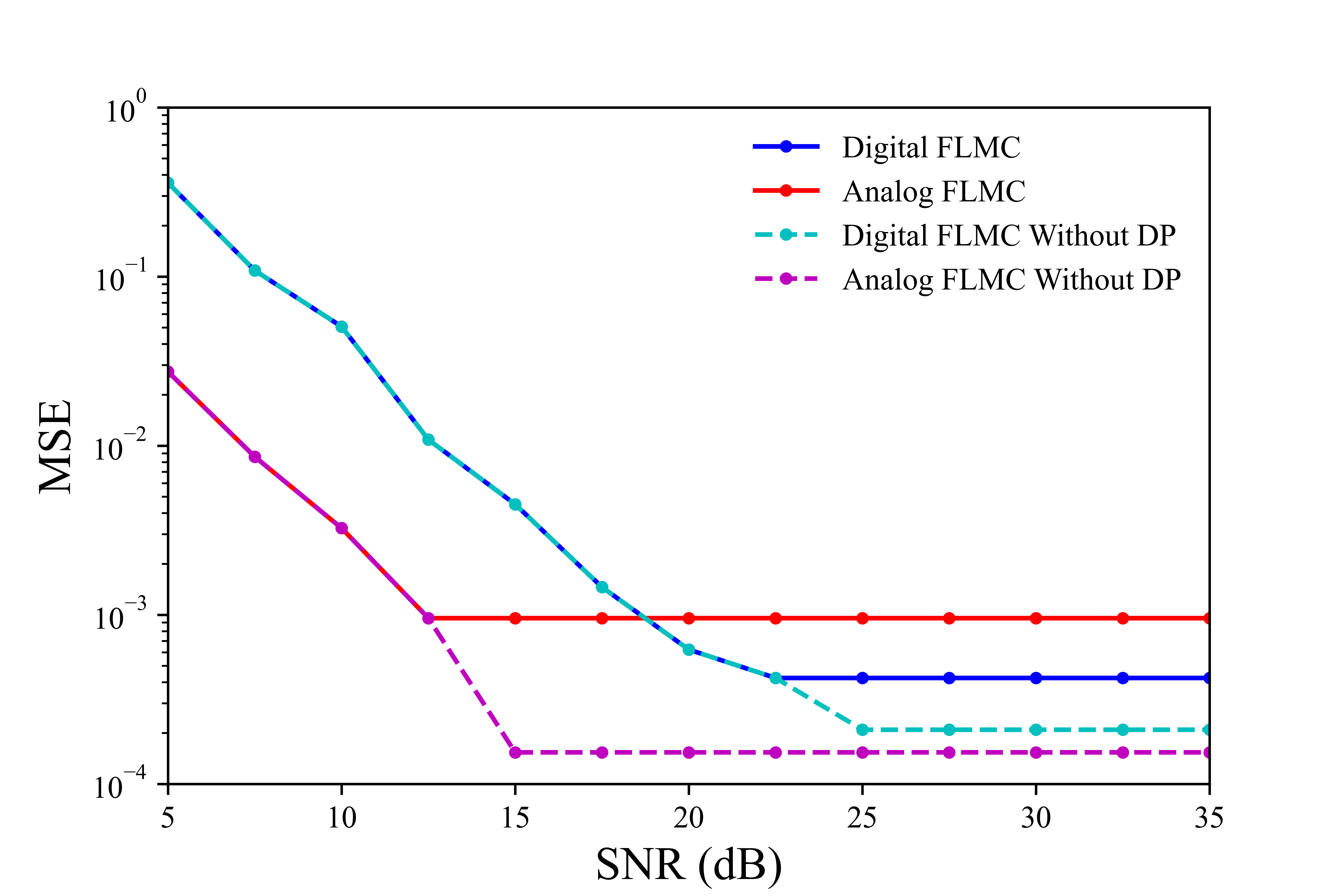
Figure 2: MSE as a function of SNR ($\epsilon=5,\delta=0.01$).

We now further investigate the impact of the privacy level on the digital and analog FLMC schemes in Fig. 3. In this experiment, we set $\mathsf{SNR}_{\sf max}=25$ dB. The error of all schemes is seen to decrease by relaxing the DP constraint, until $\epsilon=7.5$ for the digital scheme and $\epsilon=15$ for the analog scheme. Relaxing the DP constraint cannot reduce the error, as the performance becomes limited by the transmitted power constraint or by LMC noise requirement. The digital FLMC scheme outperforms analog FLMC under a stricter DP requirement, i.e., when $\epsilon\leq 7.5$. This provides further validation of the advantage of the digital scheme when the SNR is large enough.

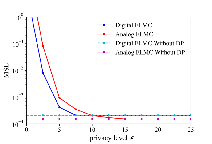
Figure 3: MSE as a function of privacy level $\epsilon$ ($\mathsf{SNR}_{\sf max}=25$ dB, $\delta=0.01$).

Finally, in Fig. 4, we study the impact of varying the parameter $a$ of the quantization probability function $\Phi(x)=[1+\exp(-ax)]^{-1}$. Note that a small $a$ implies a more noisy quantizer. In this experiment, we also set $\mathsf{SNR}_{\sf max}=25$ dB. Under strict DP requirement $\epsilon<2$, the quantizer with the small value $a=0.01$ outperforms other choices, since the higher level of randomness is applied to meet the DP constraint. Conversely, by relaxing the DP requirement, quantizer with larger value of $a$ become advantageous.

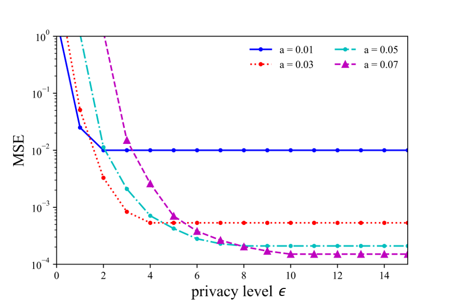
Figure 4: MSE as a function of privacy level $\epsilon$ for different parameter of the stochastic binary quantization $a$ ($\mathsf{SNR}_{\sf max}=25$ dB, $\delta=0.01$).

References

- [1] J. Park, S. Samarakoon, M. Bennis, and M. Debbah, “Wireless network intelligence at the edge,” Proc. IEEE, vol. 107, no. 11, pp. 2204–2239, 2019.
- [2] Z. Zhou, X. Chen, E. Li, L. Zeng, K. Luo, and J. Zhang, “Edge intelligence: Paving the last mile of artificial intelligence with edge computing,” Proc. IEEE, vol. 107, no. 8, pp. 1738–1762, 2019.
- [3] G. Zhu, D. Liu, Y. Du, C. You, J. Zhang, and K. Huang, “Toward an intelligent edge: wireless communication meets machine learning,” IEEE Commun. Mag., vol. 58, no. 1, pp. 19–25, 2020.
- [4] T. Sery, N. Shlezinger, K. Cohen, and Y. C. Eldar, “Over-the-air federated learning from heterogeneous data,” IEEE Trans. Signal Process., vol. 69, pp. 3796–3811, June 2021.
- [5] H. H. Yang, Z. Chen, T. Q. Quek, and H. V. Poor, “Revisiting analog over-the-air machine learning: The blessing and curse of interference,” [Online]. Available: https://arxiv.org/pdf/2107.11733.pdf, 2021.
- [6] M. M. Amiri and D. Gündüz, “Machine learning at the wireless edge: Distributed stochastic gradient descent over-the-air,” IEEE Trans. Signal Process., vol. 68, pp. 2155–2169, 2020.
- [7] D. Liu and O. Simeone, “Privacy for free: Wireless federated learning via uncoded transmission with adaptive power control,” IEEE J. Sel. Areas Commun., vol. 39, pp. 170–185, Nov. 2020.
- [8] X. Cao, G. Zhu, J. Xu, and S. Cui, “Optimized power control design for over-the-air federated edge learning,” [Online]. Available: https://arxiv.org/pdf/2106.09316.pdf, 2021.
- [9] G. Zhu, Y. Du, D. Gunduz, and K. Huang, “One-bit over-the-air aggregation for communication-efficient federated edge learning: Design and convergence analysis,” [Online]. Available: https://arxiv.org/pdf/2001.05713.pdf, 2020.
- [10] M. E. Khan and H. Rue, “The bayesian learning rule,” arXiv preprint arXiv:2107.04562, 2021.
- [11] K. Alwasel, D. N. Jha, F. Habeeb, U. Demirbaga, O. Rana, T. Baker, S. Dustdar, M. Villari, P. James, E. Solaiman, et al., “Iotsim-osmosis: A framework for modeling and simulating iot applications over an edge-cloud continuum,” Journal of Systems Architecture, vol. 116, p. 101956, 2021.
- [12] S. T. Jose and O. Simeone, “Free energy minimization: A unified framework for modeling, inference, learning, and optimization [lecture notes],” IEEE Signal Processing Magazine, vol. 38, no. 2, pp. 120–125, 2021.
- [13] E. Angelino, M. J. Johnson, and R. P. Adams, “Patterns of scalable bayesian inference,” [Online]. Available: https://arxiv.org/pdf/1602.05221.pdf, 2016.
- [14] D. Liu and O. Simeone, “Wireless federated Langevin monte carlo: Repurposing channel noise for bayesian sampling and privacy,” [Online]. Available: https://arxiv.org/pdf/2108.07644.pdf, 2021.
- [15] Y. Koda, K. Yamamoto, T. Nishio, and M. Morikura, “Differentially private aircomp federated learning with power adaptation harnessing receiver noise,” [Online]. Available: https://arxiv.org/pdf/2004.06337.pdf, 2020.
- [16] D. Liu and O. Simeone, “Privacy for free: Wireless federated learning via uncoded transmission with adaptive power control,” IEEE Journal on Selected Areas in Communications, vol. 39, no. 1, pp. 170–185, 2021.
- [17] D. Gündüz, P. de Kerret, N. D. Sidiropoulos, D. Gesbert, C. R. Murthy, and M. van der Schaar, “Machine learning in the air,” IEEE Journal on Selected Areas in Communications, vol. 37, no. 10, pp. 2184–2199, 2019.
- [18] B. Nazer and M. Gastpar, “Computation over multiple-access channels,” IEEE Trans. Inf. Theory, vol. 53, no. 10, pp. 3498–3516, 2007.
- [19] W. Liu, X. Zang, Y. Li, and B. Vucetic, “Over-the-air computation systems: Optimization, analysis and scaling laws,” IEEE Trans. Wireless Commun., vol. 19, no. 8, pp. 5488–5502, 2020.
- [20] M. Seif, R. Tandon, and M. Li, “Wireless federated learning with local differential privacy,” [Online]. Available: https://arxiv.org/pdf/2002.05151.pdf, 2020.
- [21] V. Gandikota, R. K. Maity, and A. Mazumdar, “vqSGD: Vector quantized stochastic gradient descent,” [Online]. Available: https://arxiv.org/pdf/1911.07971.pdf, 2019.
- [22] R. Jin, Y. Huang, X. He, H. Dai, and T. Wu, “Stochastic-sign sgd for federated learning with theoretical guarantees,” [Online]. Available: https://arxiv.org/pdf/2002.10940.pdf, 2020.
- [23] C. Dwork, A. Roth, et al., “The algorithmic foundations of differential privacy,” Foundations and Trends® in Theoretical Computer Science, vol. 9, no. 3–4, pp. 211–407, 2014.
- [24] X. Chen, Z. S. Wu, and M. Hong, “Understanding gradient clipping in private SGD: A geometric perspective,” [Online]. Available: https://arxiv.org/pdf/2006.15429.pdf, 2020.
- [25] Y.-X. Wang, S. Fienberg, and A. Smola, “Privacy for free: Posterior sampling and stochastic gradient Monte Carlo,” in Proc. Conf. Mach. Learning (ICML), (Lille, France), July 2015.