A New Method for the Reconstruction of Strongly Lensed Galaxies with Resolved Kinematics

Abstract

Integral field spectroscopy of high-redshift galaxies has become a powerful tool for understanding their dynamics and evolutionary states. However, in the case of gravitationally lensed systems, it has proved difficult to model both lensing and intrinsic kinematics in a way that takes full advantage of the information available in the spectral domain. In this paper, we introduce a new method for pixel-based source reconstruction that alters standard regularization schemes for two-dimensional data in a way that leverages kinematic information in a physically motivated but flexible fashion, and that is better suited to the three-dimensional nature of integral field data. To evaluate the performance of this method, we compare its results to those of a more traditional two-dimensional non-parametric approach using mock ALMA observations of a typical high-redshift dusty star-forming galaxy. We find that 3D regularization applied to an entire data cube reconstructs a source’s intensity and velocity structure more accurately than 2D regularization applied to separate velocity channels. Cubes reconstructed with 3D regularization also have more uniform noise and resolution properties and are less sensitive to the signal-to-noise ratio of individual velocity channels than the results of 2D regularization. Our new approach to modeling integral field observations of lensed systems can be implemented without making restrictive a priori assumptions about intrinsic kinematics, and opens the door to new observing strategies that prioritize spectral resolution over spatial resolution (e.g., for multi-configuration arrays like ALMA).

April 8, 2022

1 Introduction

Strong gravitational lensing stretches and amplifies the images of distant sources, making them easier to detect and resolve, and allows us to probe the mass distributions of the foreground structures that lens them. Fully exploiting the scientific potential of strong lensing requires the simultaneous reconstruction of both the intrinsic source-plane structure and the lensing potential for a given system — a complex inference problem whose solution is the main goal of gravitational lens modeling. For a multiply imaged system, different features observed on the sky originate from the same part of the source; a good lens model will recover this consistency, while a bad one will not. As a result, the most robust lens models tend to be derived from data that maximize the number of distinct “features” that can be identified, i.e., the number of resolution elements spanning the observed source. In the context of imaging, this criterion translates to high angular resolution, explaining why the Hubble Space Telescope, ground-based telescopes equipped with adaptive optics, and very long baseline interferometric arrays have made important contributions to strong lensing studies. However, it is also possible to satisfy this criterion using data with high spectral resolution, which is essentially equivalent to high angular resolution for sources with large velocity gradients. As noted in previous studies of unlensed sources (e.g., Scoville et al., 1997), in fact, the angular shifts of emission centroids between adjacent velocity channels scale as $\Delta\theta\propto\Delta v\,(dv/dr)^{-1}$ — so datasets with high spectral resolution (small $\Delta v$) can provide information on scales smaller than the nominal angular resolution element. Leveraging such information may be especially effective at radio wavelengths, where heterodyne detection delivers high spectral resolution as a matter of course.

The potential value of high spectral resolution for lens modeling only adds to the scientific appeal of integral field (i.e., three-dimensional, 3D) observations of high-redshift galaxies. Spatially resolved studies of ionized and molecular gas kinematics have been used to extract rotation curves for galaxies at $z\geq 2$, which can be used to constrain their dark matter density profiles and their formation histories (e.g., Genzel et al., 2017, 2020; Rizzo et al., 2021). Spatially resolved spectral line mapping in $z\geq 2$ systems can reveal the morphology of star formation (e.g., Jones et al., 2010), the impact of gas inflow on chemical enrichment (e.g., Cresci et al., 2010), and the influence of active galactic nuclei on their surroundings (e.g., Sharon et al., 2019). When such analyses of “data cubes” (with one spectral and two spatial dimensions) are undertaken for lensed systems, they immediately benefit from the higher signal-to-noise ratios (S/Ns) and higher effective linear resolutions that lensing affords. However, if the rich information contained in the cubes can also be harnessed to improve the quality of the lens models themselves, the payoff will be even bigger.

This paper is motivated by the need for a new method of source-plane reconstruction of intrinsically 3D datasets that more fully captures the information available in those datasets in a way that previous methods do not. The work builds on a long history of methods for simultaneously reconstructing the source-plane structure and lens potential. Kochanek & Narayan (1992) combined lens modeling with the Clean algorithm for source reconstruction. Wallington et al. (1996) introduced the idea of using regularization (a prior in the Bayesian interpretation) that effectively tunes the number of source parameters and penalizes source models that are too complex, specifically employing the maximum entropy method. Warren & Dye (2003) pointed out that making the penalty function quadratic in the source surface brightness led to a fast “semi-linear” method. Several choices of quadratic regularization schemes exist, with the most common penalizing the sum of either the squared pixel values, their squared gradient, or their squared Laplacian. There is no objective standard for the choice of regularization scheme in general. Suyu et al. (2006) compared Bayesian evidences and showed that the optimal choice of prior depends on both the data and the nature of the unlensed source. Non-parametric source reconstruction methods have been further developed under a unified Bayesian framework (Brewer & Lewis, 2006) to include adaptive and irregular source plane grids (Dye & Warren, 2005; Vegetti & Koopmans, 2009) or to reconstruct a source in a shapelet basis (Birrer et al., 2015; Tagore & Jackson, 2016).

To date, the majority of strong lensing studies have focused on 2D surface brightness data. For 3D data cubes, one approach is to simply reconstruct a data cube’s channels as a series of independent sources using the 2D techniques described above (e.g., Stark et al., 2008), with no prior on how the reconstructed channels should relate to each other. This approach neglects the fact that the channels are, in fact, not unrelated to each other for any plausible kinematic state. As we discuss below, this choice often amounts to a sub-optimal regularization scheme, depending on the quality of the data. For sources that are rotating disks, the derived source plane channel images can, if desired, be fit with an analytic rotating disk model (e.g., Geach et al., 2018). However, this and other analyses of independent channel reconstructions are complicated by the non-uniform resolution and noise properties in the source plane.

In recent years, several authors have developed approaches to the reconstruction of lensed sources from integral field data. Patrício et al. (2018) fit observations to kinematic models that have been lensed into the image plane, but only fit to the velocity maps, not the full data cube. Rizzo et al. (2018) present a method for the non-parametric reconstruction of a full 3D data cube in which regularization makes use of a parameterized rotating disk model. Chirivì et al. (2020) also fit a dynamical model in the source plane, but use axisymmetric Jeans modeling to fit the kinematic moments of mock integral field observations of stellar absorption. These approaches all address the issue of non-uniform source-plane resolution and allow for (i) simultaneous optimization of lens and source parameters, and (ii) exploration of degeneracies between model parameters. However, while parameterized kinematic models can be useful in many cases, sources with disturbed kinematics, complicated morphologies, and/or multiple components can deviate significantly from such simple descriptions, and require less strict assumptions (e.g., merely the existence of velocity coherence) for the sources’ true properties to be recovered.

Convolutional neural networks and related deep learning techniques have recently begun to show promise for solving these and other related problems in lens modeling. Although generally only trained on data using singular isothermal ellipsoid (SIE) mass distributions, models have been developed to predict lens parameters and their errors from an image (Hezaveh et al., 2017; Perreault Levasseur et al., 2017). Other models have also been effective at reconstructing source-plane structure from lensed data, showing some degree of generalizability, and even achieving better results than maximum likelihood methods (Morningstar et al., 2019). Because the choice of training data for these networks imposes a prior on the reconstructed sources, we may require new models specifically designed for 3D data cubes, in which the S/N of each channel is typically much lower than for integrated moment maps and valuable information can be extracted from the spectral dimension. The large set of realistic mock data cubes needed for training in this case will be more difficult to produce than training data needed to support the reconstruction of 2D images.

In this paper we introduce a new nonparametric method for reconstructing integral field spectroscopy of lensed galaxies that addresses the above issues. This method is flexible in that it only assumes that the source kinematics are ordered, but does not require that the emitting gas follow any particular spatial or velocity distribution. The approach is a direct extension of the existing 2D nonparametric Bayesian formalism, adapted to fitting all the channels of a data cube simultaneously. In order to appropriately model a source, we introduce a new regularization scheme that is better suited to the form of the data and the properties of the source.

This paper is organized as follows. In Section, 2 we present the modified source reconstruction formalism. We describe the mock observations in Section 3. In Section 4, we compare reconstructions produced with our new method to the existing 2D nonparametric approach. Section 5 provides a summary and discusses future work.

2 Bayesian Framework

The Bayesian framework for reconstructing lensed sources allows priors to be placed on the source parameters using a regularization term that disfavors unphysical models that overfit the data, while still maintaining a flexible, non-parametric description of the source. Our new method for reconstructing sources with resolved kinematics modifies the existing Bayesian framework by treating the set of channel images as a single source in the three dimensions of the data cube, rather than modeling the channel images as a set of independent observations. This approach is implemented by reformulating the prior on the source parameters (i.e., the regularization term) to relate the channel images in a physically realistic way. Currently used priors generally restrict the smoothness of the reconstructed source in each channel image independently. The method detailed below instead enforces a restriction on the smoothness of the entire 3D surface brightness distribution in the data cube. We refer to approaches that treat the channel images as independent as 2D regularization methods, and approaches that model all of the channels of the cube together, such as the one introduced here, as 3D regularization methods.

In this section, we summarize the existing 2D regularization approach for single images, its generalization to multiple images, and finally our changes to the formalism to incorporate all of the spectral information available in the data. The general Bayesian formalism is detailed in Warren & Dye (2003), Suyu et al. (2006), and Vegetti & Koopmans (2009), while the details of our particular (2D) implementation are discussed in Tagore & Keeton (2014) and Tagore & Jackson (2016).

2.1 Existing 2D Bayesian Framework

First, we briefly review how the Bayesian formalism operates when a single lensed image is reconstructed. Let the data be represented as a 1D vector $\bm{d}$ with components $d_{k}$, where $k=1,...,N_{d}$ and $N_{d}$ is the number of data points. The data vector can be constructed by concatenating rows of pixels from the image into a 1D vector. The data vector is related to the vector of source parameters $\bm{s}$ by

$$\bm{d}=\bm{L}\bm{s}+\bm{n},$$ (1)

where $\bm{L}$ is the lensing operator and $\bm{n}$ is the noise in the observed data. The lensing operator maps source parameters to image-plane (data) pixel values and is defined to include the effects of both lensing and blurring due to an observational point-spread function (PSF). The source vector may be represented in multiple ways. The most straightforward is as a series of surface brightness values on a grid (regular or irregular); however, the surface brightness can also be defined via a set of basis functions (such as shapelets; see Refregier, 2003; Birrer et al., 2015; Tagore & Jackson, 2016), in which case the source parameters become a set of coefficients. We have restricted the scope of this work to grid-based reconstructions, although in principle an approach similar to the one described below can be applied to a shapelet-based source. We note that this formalism can also be applied to visibility-based data, which can be modeled using the same source representations.

2.1.1 Most Likely Source

The most likely source can be obtained by finding the set of source parameters that maximizes the likelihood given by

$$P(\bm{d}|\bm{L},\bm{s})\propto\exp\left(-E_{d}(\bm{d}|\bm{L},\bm{s})\right),$$ (2)

where

$$E_{d}(\bm{d}|\bm{L},\bm{s})=\frac{1}{2}\chi^{2}(\bm{s})=\frac{1}{2}\left(\bm{L}\bm{s}-\bm{d}\right)^{\top}\bm{C}_{\textrm{d}}^{-1}\left(\bm{L}\bm{s}-\bm{d}\right),$$ (3)

and $\bm{C}_{\textrm{d}}$ is the covariance matrix. Suyu et al. (2006) give the solution for the most likely source vector as

$$\bm{s}_{\text{ML}}=\bm{F}^{-1}\bm{D},$$ (4)

where $\bm{F}\equiv\bm{L}^{\top}\bm{C}_{\textrm{d}}^{-1}\bm{L}$ and $\bm{D}\equiv\bm{L}^{\top}\bm{C}_{\textrm{d}}^{-1}\bm{d}$.

2.1.2 Most Probable Source

In the presence of noise, the most likely solution tends to overfit the data, yielding an unphysical source surface brightness distribution. Writing out the full Bayesian posterior probability distribution allows us to place priors on the reconstructed source that effectively smooth the derived source and prevent overfitting. The posterior is given by

$$P(\bm{s}|\bm{d},\bm{L},\lambda,\bm{R})\propto\exp\left(-M(\bm{s}))\right),$$ (5)

where

$$M(\bm{s})\equiv E_{d}(\bm{s})+\lambda E_{s}(\bm{s}),$$ (6)

and

$$E_{s}(\bm{s})=\frac{1}{2}\bm{s}^{\top}\bm{R}\bm{s}$$ (7)

is a penalty function that enforces the priors that regularize the source parameters, and $\lambda$ is the “regularization strength,” which controls the relative contributions of the two terms in Equation 6. When $\lambda$ is large, $E_{s}(\bm{s})$ prevents the source from overfitting to the data by forcing it to be smooth; when $\lambda$ is small, the source becomes more complex in order to better fit the data. For computational efficiency, the penalty function must be expressible as a quadratic form as in Equation 7, and the regularization matrix $\bm{R}$ must be both symmetric and invertible. (This approach to fitting is known generally as Tikhonov regularization (Tikhonov et al., 1995) or ridge regression, although applications in most other contexts often use $\bm{R}\equiv\bm{I}$.) These conditions restrict our choice of a new regularization matrix in Section 2.2.

The matrix $\bm{R}$ is defined according to the specific regularization scheme. Common choices compute the square of the surface brightness gradient or Laplacian summed over all of the pixels, roughly corresponding to the expectation that a realistic surface brightness distribution should be relatively smooth. We emphasize here that the regularization schemes are somewhat arbitrary; most reasonable choices do similarly well at mitigating the overfitting problem but produce differences in the reconstructed sources. For example, zeroth-order ($\bm{R}=\bm{I}$) regularization biases a source toward a “zero” (featureless) source; first-order (gradient-based) regularization biases toward a constant-value source; and second-order (Laplacian-based) regularization biases toward a planar source.

The most probable source vector $\bm{s}_{\text{MP}}$ maximizes Equation 5. For a given value of $\lambda$, the most probable source is given by Suyu et al. (2006) as

$$\bm{s}_{\text{MP}}=\bm{A}^{-1}\bm{F}\bm{s}_{\text{ML}},$$ (8)

where $\bm{A}=\bm{F}+\lambda\bm{R}$. However, to find the best estimate of the source vector, we must find the optimal value of $\lambda$. This step can be done (see Suyu et al. 2006) by maximizing the posterior for $\lambda$:

$$P(\lambda|\bm{d},\bm{L},\bm{R})\propto P(\bm{d}|\lambda,\bm{L},\bm{R})P(\lambda).$$ (9)

The prior is typically assumed to be uniform in $\log\lambda$ because the scale of $\lambda$ is not known a priori.

Formally, the most probable source is found by marginalizing over $\lambda$; however, Equation 9 is sharply peaked and can be well approximated by a delta function. As a result, simply using the value of $\lambda$ that maximizes the posterior works well in practice. Suyu et al. (2006) discuss this issue in more detail and give the equation to maximize to find $\lambda$ (see their Equation 19).

2.1.3 Generalization to Multiple Observations

For a set of data vectors $\{\bm{d}_{i}\}$ comprising $N_{c}$ images, e.g., as obtained in multiple filters or multiple velocity channels, the most general form of Bayes’s theorem is

$$P(\{\bm{s}_{i}\}|\{\bm{d}_{i}\},\bm{L},\{\lambda_{i}\},\bm{R})\propto P(\{\bm{d}_{i}\}|\{\bm{s}_{i}\},\bm{L})$$ (10)

$$\times P\left(\{\bm{s}_{i}\}|\{\lambda_{i}\},\bm{R}\right).$$

On the right-hand side, the first term is the likelihood for all of the data, while the second term is a prior over all of the source parameters.

For simplicity, we assume throughout this paper that the data points in each observation correspond to the same sets of pixels (i.e., the pixelization is the same and the same mask is applied to all images) so that each observation uses the same lensing operator $\bm{L}$. It follows straightforwardly from Equation 3 that the full likelihood can be factored into a product of likelihoods for individual images or channels:

$$P(\{\bm{d}_{i}\}|\{\bm{s}_{i}\},\bm{L})=\prod_{i=1}^{N_{c}}P(\bm{d}_{i}|\bm{s}_{i},\bm{L}).$$ (11)

The prior can be written in several different ways. The simplest is as a product of factors for the individual images/channels:

$$P\left(\{\bm{s}_{i}\}|\{\lambda_{i}\},\bm{R}\right)=\prod_{i}P\left(\bm{s}_{i}|\lambda_{i},\bm{R}\right).$$ (12)

This approach is equivalent to treating each of the observations as independent. The most probable set of source channel images $\{\bm{s}_{i}\}$ is then found by maximizing the posterior for each $\lambda_{i}$ independently. For a set of observations in several photometric filters, this approach is likely the best one in the absence of a model relating the emission across the filters. If the data are closely spaced channels in a data cube from an integral field spectrograph or a radio telescope, however, the emission in consecutive channels is related by the source kinematics, making it non-optimal to treat the channels independently. The next section lays out a more informed way of writing the prior for sources with resolved kinematics.

2.2 Updated 3D Bayesian Framework

We assume here that (i) our data are a set of channel images from a data cube with uniform angular resolution, and (ii) the channels have the same masks applied, such that each pixel that exists in any channel image exists in every channel image. The latter assumption ensures that we can reconstruct using source plane grids that are identical for all channels. We can then define the vector $\bm{d}$ for all of the data points $\{\bm{d}_{i}\}$ as the concatenation of all of the data vectors for each of the channel images. We choose to continue to describe the source as a set of channel images, so that the source vector $\bm{s}$ can be defined similarly. (In principle, the source vector can be defined in an alternative way, e.g., using a set of 3D basis functions, but such a scenario is beyond the scope of the present paper.)

Throughout this section, we represent matrices that act on the vector of combined data cube images with a hat, e.g., $\bm{\hat{L}}$. Unless otherwise defined, these are block-diagonal matrices formed by $N_{c}$ blocks of the original matrix. For example, $\bm{\hat{L}}\equiv\bm{I}_{N_{c}}\otimes\bm{L}$, where $\bm{I}_{N_{c}}$ is the $N_{c}\times N_{c}$ identity matrix and $\otimes$ denotes the Kronecker product. Following this notation, the likelihood, which can be factored as in Equation 11, can instead be written as in Equation 2 after replacing un-hatted matrices with their hatted counterparts:

$$E_{d}(\bm{d}|\bm{s},\bm{\hat{L}})=\frac{1}{2}\left(\bm{\hat{L}}\bm{s}-\bm{d}\right)^{\top}\bm{\hat{C}}_{\textrm{d}}^{-1}\left(\bm{\hat{L}}\bm{s}-\bm{d}\right).$$ (13)

The block-diagonal form of $\bm{\hat{L}}$ persists as long as adjacent channels are independent, since $\bm{L}$ only includes blurring by the 2D PSF. This assumption holds for radio data, which we consider in this work, but not for some shorter-wavelength data where a line-spread function (LSF) means adjacent channels are not independent. Appendix A discusses how the $\bm{\hat{L}}$ matrix can be changed to account for an LSF in such cases.

2.2.1 3D Regularization

As discussed above, the 2D regularization schemes allow us to reconstruct a relatively smooth source in 2D without prescribing a particular emission profile. Nevertheless, the specific choice of regularization matrix influences the properties of the source. A rigorous Bayesian analysis incorporates variation of priors in order to understand the effect of prior choice on the results. This fact motivates us to reformulate our prior (the regularization matrix) in order to better reflect the expected properties of the source in 3D. This matrix should impose a similar spatial smoothness constraint on the reconstruction while also requiring that emission change smoothly from one channel to the next. We do this by defining a new regularization matrix that penalizes the squared 3D gradient (or Laplacian) of the source summed over all pixels in the source data cube.

In contrast to Equation 12, we write the prior for the 3D regularization in the form

$$P(\{\bm{s}_{i}\}|\{\lambda_{i}\},\bm{R}) =P(\bm{s}|\bm{\hat{R}_{\text{3D}}}(\lambda,\eta))$$

$$\propto\exp\left(-\frac{1}{2}\bm{s}^{\top}\bm{\hat{R}_{\text{3D}}}\bm{s}\right),$$ (14)

where $\bm{\hat{R}_{\text{3D}}}(\lambda,\eta)$ is the new 3D regularization matrix and we use only two regularization strengths, $\lambda$ and $\eta$. Note that we have absorbed $\lambda$ and $\eta$ into the regularization matrix, which we define below.

The 2D regularization matrix for a single channel image is given by $\bm{R_{\text{2D}}}=\bm{H_{\text{2D}}}^{\top}\bm{H_{\text{2D}}}$, where $\bm{H_{\text{2D}}}$ is the matrix that computes the components of the gradient (or Laplacian) for all of the pixels in the source. Similarly, the 2D regularization matrix for a set of channel images is given by $\bm{\hat{R}_{\text{2D}}}\equiv\bm{\hat{H}_{\text{2D}}}^{\top}\bm{\hat{H}_{\text{2D}}}$, where $\bm{\hat{H}_{\text{2D}}}=\bm{I}_{N_{c}}\otimes\bm{H_{\text{2D}}}$. We can similarly define the matrix $\bm{\hat{H}_{\text{3D}}}$ that computes the components of the gradient (or Laplacian) in 3D as

$$\bm{\hat{H}_{\text{3D}}}\equiv\lambda^{1/2}\bm{\hat{H}_{\text{2D}}}+\eta^{1/2}\bm{\hat{Q}},$$ (15)

where $\bm{\hat{Q}}$ contains the extra terms that specify the components of the gradient or Laplacian in the third dimension. Appendix B provides a derivation of $\bm{\hat{Q}}$ for both of these cases. The 3D regularization matrix is then

$$\bm{\hat{R}_{\text{3D}}} \equiv\bm{\hat{H}_{\text{3D}}}^{\top}\bm{\hat{H}_{\text{3D}}}$$

$$=\lambda\bm{\hat{R}_{\text{2D}}}+\eta\bm{\hat{Q}}^{\top}\bm{\hat{Q}}$$

$$\quad+\lambda^{1/2}\eta^{1/2}\left(\bm{\hat{H}_{\text{2D}}}^{\top}\bm{\hat{Q}}+\bm{\hat{Q}}^{\top}\bm{\hat{H}_{\text{2D}}}\right).$$ (16)

When $\eta=0$, this regularization scheme reduces to the 2D case with $\lambda$ identical for all channels.

We have introduced a second regularization strength, $\eta$, to control the smoothness of the reconstruction in the spectral direction, analogous to how $\lambda$ controls its spatial smoothness. We refer to $\lambda$ and $\eta$ as the spatial and spectral regularization strengths, respectively. It is necessary to have two such strengths because the spatial and spectral dimensions of the cube have different units and independent smoothness requirements.

In the 2D context, it is well understood that regularization affects the properties of the reconstructed source. The addition of the regularization term results in a biased estimator of the real source, in the sense that the reconstruction mitigates the effect of the noise in the data by introducing correlations between neighboring source-plane pixels. The scale over which this spatial correlation is present is determined by the regularization strength, such that larger values of $\lambda$ cause correlations over larger scales. Likewise, the 3D regularized source is also a biased estimator, but with correlations now present in both the spatial and spectral directions, on scales determined by the two regularization strengths. We will see in Section 4.2 how this bias affects the reconstructed sources.

2.2.2 Most Probable Source

For given values of $\lambda$ and $\eta$, the most likely source, $\bm{s}_{\text{ML}}$, is given by Equation 4 with the matrices replaced by their hatted versions. Likewise, the most probable source is given, analogous to Equation 8, by

$$\bm{s}_{\text{MP}}=\bm{\hat{A}}^{-1}\bm{\hat{F}}\bm{s}_{\text{ML}},$$ (17)

where we now have $\bm{\hat{A}}=\bm{\hat{F}}+\bm{\hat{R}_{\text{3D}}}(\lambda,\eta)$

2.2.3 Finding $\lambda$ and $\eta$

As in the 2D regularization case, the joint posterior for $\lambda$ and $\eta$ is given by

$$P(\lambda,\eta|\bm{d},\bm{\hat{L}},\bm{\hat{R}_{\text{3D}}})\propto P(\bm{d}|\lambda,\eta,\bm{\hat{L}},\bm{\hat{R}_{\text{3D}}})P(\lambda,\eta).$$ (18)

In order to compute the posterior, we must place a prior on the regularization strengths, $P(\lambda,\eta)$. As in the 2D case, we do not know the scale for either regularization strength a priori, and it is natural to assume that both $\lambda$ and $\eta$ have log-uniform priors. Consequently, maximizing Equation 18 is equivalent to maximizing $\ln P(\bm{d}|\lambda,\eta,\bm{\hat{L}},\bm{\hat{R}_{\text{3D}}})$.

Following the same steps as Suyu et al. (2006), we can derive the joint posterior for the regularization strengths as

$$\ln P(\lambda,\eta|\bm{d}) =\frac{1}{2}\ln\lvert\bm{\hat{R}_{\text{3D}}}\rvert-\frac{1}{2}\ln\lvert\bm{\hat{A}}\rvert$$

$$\quad+\frac{1}{2}\bm{s}_{\text{MP}}\bm{\hat{A}}\bm{s}_{\text{MP}}-\frac{1}{2}\ln\lvert\bm{\hat{C}}_{\textrm{d}}\rvert$$

$$\quad-\frac{N_{d}N_{c}}{2}\ln 2\pi.$$ (19)

This equation is analogous to Equation 19 in Suyu et al. (2006), but with the vectors and matrices replaced with their larger, hatted versions.

As with the 2D approach, we can maximize Equation 2.2.3 to find the optimal pair of regularization strengths. Again, we want to marginalize over the regularization strengths; however, we still expect the posteriors to be sharply peaked enough that we can use the modes in place of the marginalized distributions. We explore this assumption in Section 4.2.1.

3 Mock Observations

To compare the performance of our new approach to that of existing methods, we create a series of mock observations of carbon monoxide (CO) line emission from galaxy disks at redshift $z\sim 2$–$3$, as would be observed by the Atacama Large Millimeter/submillimeter Array (ALMA). Since our source representation is flexible, we expect that the results of the tests discussed below are not strongly dependent on the chosen parameters of the disk models used to generate the mock observations.

Briefly, the mock data cubes are created as follows. The unlensed source cubes are produced using the Python package GalPaK${}^{\text{3D}}$ (Bouché et al., 2015), which generates data cubes from parameterized models of rotating disks. We then use the lens modeling software lensmodel (Keeton, 2011) to lens the source channel images. Finally, we convolve the channel images with a synthesized beam and add noise to simulate mock observations. The following subsections describe these steps in more detail; as discussed in Section 4, we have especially focused on exploring the effects of the spectral and spatial resolutions and the S/N ratio of the observations.

3.1 Input Source Models

GalPaK${}^{\text{3D}}$ allows the functional forms of several components of a disk model to be changed: the galaxy flux profile, disk thickness profile, rotation curve shape, and dispersion profile. Because our lens modeling approach is non-parametric, we expect choices among these options to have little effect on the quality of our reconstructions. Therefore, we leave them fixed at their defaults: an exponential flux profile, Gaussian thickness profile, $\arctan$ rotation curve, and “thick” dispersion profile.

Each source cube used as input to lensmodel is defined by its dimensions, its spatial and spectral resolutions, and the 10 parameters of a disk model (positional center, $x_{0}$, $y_{0}$; reference velocity, $v_{z_{0}}$; half-light radius, $R_{1/2}$; inclination angle, $\theta_{\text{inc}}$; position angle, PA; turnover radius, $r_{t}$; maximum velocity, $V_{\text{max}}$; velocity dispersion, $\sigma_{0}$; and overall normalization). The pixel scale of the input source is chosen to be small enough that it does not affect the pixel values in the final lensed image. The final spectral resolution is set when the mock cube is created, while the final spatial resolution is set after the mock images are lensed.

3.2 Simulated Observations

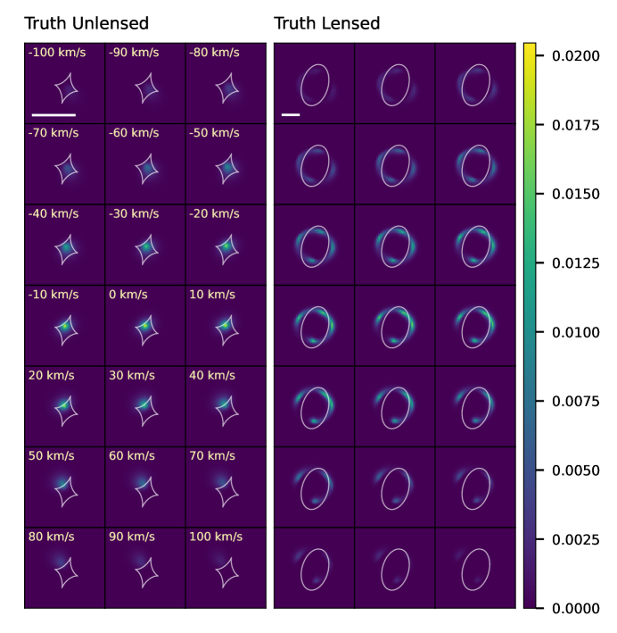
Figure 1: Example of the channel images for the “true” unlensed (left) and lensed (right) source used to make the mock observations. The channel width for this example is $10\,\text{km}\,\text{s}^{-1}$. The lensed images are shown with no noise and no convolution with a synthesized beam. The scale bars show $1^{\prime\prime}$. The critical curve and caustic are shown in white. The velocity of each channel is shown in the upper left. The color scale shows arbitrary surface brightness units.

After creating a data cube of the unlensed source, we use lensmodel to lens each of the channel images, choosing lens model parameters that are typical of observed lensed systems. For most examples in this paper, we use as a fiducial lens model a singular isothermal ellipsoid with an Einstein radius $b=1^{\prime\prime}$, ellipticity $e=0.38$, position angle $-16^{\circ}$, and no external shear. The image plane channel maps (before convolution) are created by interpolating surface brightness values between source-plane pixels. The pixel scale of the lensed channel images is chosen to achieve the desired resolution when convolved with a circular Gaussian beam with a FWHM of 5 pixels. After convolving with the beam, we add uniform Gaussian noise across all channels to achieve a desired S/N for the mock observations.

It should be noted that the position of the source and the orientation of its velocity gradient with respect to the caustic can be expected to have some effect on the comparison between regularization approaches. For a source–lens configuration in which the velocity gradient crosses or closely approaches the caustic, the source channel images will effectively cover a larger number of very different source–lens configurations, providing many constraints on the lens potential. This effect is illustrated in Figure 1, which shows how the unlensed channel images are lensed into a series of different configurations because of the large source velocity gradient.

The fiducial data set used throughout this paper is created using the lens model given above and a source model with parameters chosen to be typical for high-redshift galaxies: $R_{1/2}=1.6\,\text{kpc}\,(0.2^{\prime\prime})$, $\theta_{\text{inc}}=45^{\circ}$, $r_{t}=1.6\,\text{kpc}\,(0.2^{\prime\prime})$, $V_{\text{max}}=150\,\text{km}\,\text{s}^{-1}$, and $\sigma_{0}=30\,\text{km}\,\text{s}^{-1}$. This model corresponds to a dynamical mass of $M_{\text{dyn}}=V_{\text{max}}^{2}R_{1/2}/G=8.4\times 10^{9}\,M_{\odot}$. The final data cube has $10\,\text{km}\,\text{s}^{-1}$ channels, a $0.5^{\prime\prime}$ FWHM beam, and a peak S/N of 30. These channel images are shown in Figure 1 before convolution with the beam and inclusion of noise.

4 Comparison between Approaches

4.1 Implementation

We modify the source reconstruction package pixsrc (Tagore & Keeton, 2014; Tagore & Jackson, 2016), which is an extension to the lensmodel code (Keeton, 2011), to perform the lens modeling and source reconstruction described in Section 2 above. We compare the performance of the 2D and 3D regularization approaches below but first discuss some aspects of the computations here.

In the tests throughout this paper we use a grid that is constructed by ray-tracing every third data pixel back to the source plane. For our $51\times 51$ pixel data images, these settings with the fiducial lens model result in a total of $873$ pixels to describe one image of the source. Our fiducial $21$ channel dataset thus requires a total of $18,333$ free parameters to describe the entire source-plane cube. Source-plane images throughout this paper are produced by interpolating the irregular source-plane pixel values onto a grid of smaller square “visualization pixels.” The size of the visualization pixels is the pixsrc default of $1/4$ the data pixel size.

For ease of comparison with the bulk of the lensing literature, we use Laplacian-based regularization. The $\bm{\hat{R}_{\text{3D}}}$ matrix described above is very sparse for data with even a few channels. The $\bm{\hat{H}_{\text{2D}}}$ matrix is block-diagonal and built up from copies of $\bm{H_{\text{2D}}}$, which itself is sparse, and $\bm{\hat{Q}}$ has only three non-zero diagonals (see Appendix B). As a result, we can efficiently solve matrix equations and compute determinants using existing sparse matrix libraries that can take advantage of multi-threaded processors. We use scikit-sparse, which provides a python interface to the CHOLMOD library (Chen et al., 2008), for sparse matrix calculations. Nevertheless, the matrices are still quite large ($\bm{\hat{A}}$ is $N_{s}N_{c}\times N_{s}N_{c}$), and computation times may be a potential concern for datasets with a very large number of channels.

Finding the optimal regularization strength consumes a significant fraction of the computation time even when using 2D regularization. Because of the large matrices and the fact that we are now searching for two optimal regularization strengths, identifying a local minimum becomes more of a problem for 3D regularization. We have not yet explored methods for speeding up this parameter search.

In the tests below, we fix the lens model to the true one used in generating the mock observations. The likely approach for modeling real data would be to derive an initial lens model from the zeroth-moment map and use this as a starting point for further modeling of the full data cube. This two-step approach should cut down significantly on computation time compared to a full lens model optimization with 3D regularization. We defer to a future paper an investigation of the effects of our approach on the final derived lens model parameters and corresponding source intensity distribution.

4.2 Behavior and Performance

We perform most of our comparisons using the fiducial source and lens models described in Section 3.2 for a mock dataset with $0.5^{\prime\prime}$ spatial resolution, $10\,\textrm{km}\,\textrm{s}^{-1}$ spectral resolution, and a peak S/N radio of 30. We vary these observational parameters in Sections 4.2.4 and 4.2.5 to assess their effects on the reconstruction properties.

4.2.1 Optimization of regularization strengths

Figure 2: Views of the regularization strength posterior probability distribution. Lower left: full posterior distribution $P(\lambda,\eta)$ with the peak from the numerical optimization, $(\lambda_{\rm best},\eta_{\rm best})$, marked with a black X. The contour levels are 20%, 40%, 60%, and 80% of the peak. The two conditional posteriors are shown, (above) $P(\lambda,\eta_{\rm best})$ and (right) $P(\lambda_{\rm best},\eta)$. Note the small ranges of regularization strengths.

The optimal regularization strengths can be found by optimizing the posterior given in Equation 2.2.3. In order to account for correlations between pixels in the images, we use the noise scaling procedure described in Riechers et al. (2008). Without noise scaling, the reconstructed sources produce residuals with an RMS significantly lower than the data noise level. To produce an appropriately smooth source, we scale the input noise level by a factor that results in residuals with the expected RMS value. Because this noise scale factor should be dependent on properties of the data, we determine its value using 3D regularization and fix it for all other regularization schemes with the same data.

As discussed above, we expect that the 3D regularization strength posterior should be narrow as in the 2D case (Suyu et al., 2006), allowing a simple optimization of the regularization strengths to determine the best source. We test this expectation by plotting the posterior for the two 3D regularization strengths in Figure 2. The lower left panel shows the joint posterior $P(\lambda,\eta)$ for the fiducial dataset, while the upper left and lower right panels show the conditional posteriors $P(\lambda,\eta_{\rm best})$ and $P(\lambda_{\rm best},\eta)$, respectively. The optimal values of the regularization strengths were found to be $(\log\lambda_{\rm best},\log\eta_{\rm best})=(3.94,6.56)$, and the standard deviations of the conditional posteriors were $(\sigma_{\log\lambda},\sigma_{\log\eta})=(0.06,0.03)$. We then reconstruct sources two standard deviations (in log-space) from the peak on either side of each conditional posterior distribution with the other regularization strength fixed to the best value. We find that these sources deviate by no more than $\sim 3\%$ of the peak of the best source. This indicates that the posterior is narrow compared with the scale over which the reconstructed source changes appreciably, such that we can approximate sources near the peak by the best source.

4.2.2 General Reconstruction Properties

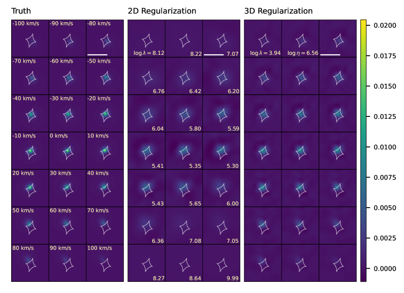
Figure 3: Comparison of the different source reconstruction techniques for the fiducial mock data cube with channel width $10\,\text{km}\,\text{s}^{-1}$. From left to right: the “true” (input) source, the reconstruction using 2D regularization, and the reconstruction using 3D regularization. The scale bars show $1^{\prime\prime}$. The caustic is shown in white. The velocity of each channel is shown at the upper left. The 2D regularization strength is shown in the lower right of each relevant panel, and the 3D regularization strengths are shown in the first two panels for the 3D regularized source. The 3D reconstructed sources are significantly more compact than their 2D counterparts and are detected better in the outer channels where the 2D reconstructed sources are not.

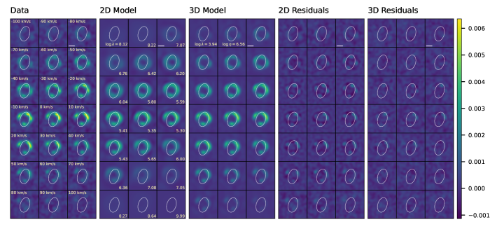
Figure 4: Comparison of the source models in the image plane. From left to right: the simulated data, the lensed 2D regularization model, the lensed 3D regularization model, the 2D regularization residuals, and the 3D regularization residuals. The residuals show that the 3D regularization gives a better fit to the observed data with residuals much closer to the noise level. The critical curve is shown in white; regularization strengths are indicated as in Figure 3.

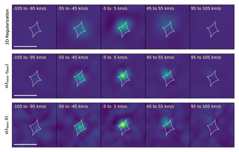
Figure 5: Comparison between sources reconstructed with different regularization schemes. Rows (top to bottom): the 2D-regularized reconstruction with regularization strengths given in Figure 3, the 3D-regularized reconstruction with optimal regularization strengths $(\lambda_{\text{best}},\eta_{\text{best}})=(10^{3.94},10^{6.56})$, and the 3D-regularized reconstruction with regularization strengths $(\lambda_{\text{best}},0)$. Each row shows five channel images selected from the reconstructed cube. The higher noise in the bottom row compared to the middle row shows how the spectral portion of the 3D regularization (i.e., the terms in $\bm{\hat{Q}}$) suppresses noise in the spectral direction.

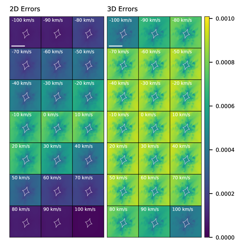
Figure 6: Source plane errors for 2D and 3D regularization. For 2D regularization, the magnitude and spatial structure of the errors depend on the value of the spatial regularization strength, $\lambda$, for each channel. For the 3D regularization, the magnitude and spatial structure of the errors is more uniform across channels (except for edge channel effects) due to the structure of the 3D regularization matrix.

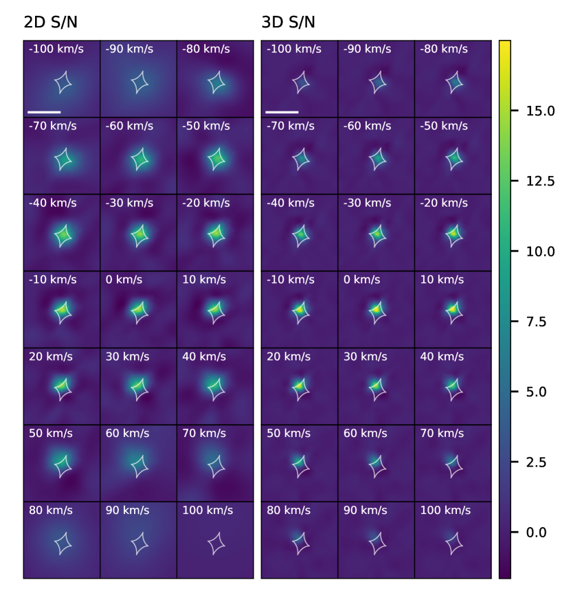
Figure 7: Maps of the source plane S/N ratio for 2D and 3D regularization. Despite the generally higher noise level of the 3D regularization shown in Figure 6, the peak S/N ratio is higher because of the higher effective resolution.

Reconstructions of the fiducial dataset using both regularization schemes are compared to the true input source in Figure 3. Figure 4 shows the mock data that are used for the reconstructions as well as the lensed and PSF blurred model images and their respective residuals. We find that the 3D regularization consistently produces source-plane channel maps that are an overall better match to the data and the true source. The source reconstructed with the new method is more compact than its 2D counterpart, with a higher peak surface brightness and an overall profile that more closely resembles that of the truth. Importantly, the 3D reconstruction also better reproduces the emission in the low-S/N outer channels where the 2D reconstruction fails. The RMS of the difference between the truth and the reconstructions is 50% higher for the 2D regularization, at 0.00031 vs. 0.00020 for the 3D regularization in arbitrary surface brightness units. (These numbers are also consistent with the error images shown in Figure 6 below.)

The more compact 3D reconstruction is the result of a smaller effective source plane beam (mostly the consequence of a smaller spatial regularization strength $\lambda$), although the effect of the new regularization scheme on the resolution and noise properties of the reconstructions is more complex. Both schemes smooth over noise and “ringing” in the maximum likelihood reconstructions by creating correlations, at the cost of a lower effective resolution. For the 3D regularization, the smoothing in the spectral direction comes from the $\eta$-terms in $\bm{\hat{R}_{\text{3D}}}$. This effect can be seen in Figure 5, which shows selected channels of the best 2D reconstruction, the best 3D reconstruction with $(\lambda,\eta)=(\lambda_{\text{best}},\eta_{\text{best}})$, and the 3D reconstruction with $(\lambda,\eta)=(\lambda_{\text{best}},0)$. The last of these shows how significantly the noise is smoothed across channel images.

Another way to view the better performance of the 3D regularization is to note the number of free parameters in each of the regularization schemes. The 2D regularization has $N_{c}=21$ regularization strengths, while the 3D regularization has only two. Despite this, the 3D regularization achieves a better fit because the regularization matrix is better suited to the data.

Because of the structure of the regularization matrices, 2D regularization produces correlations in only the spatial directions, while 3D regularization also does so in the spectral direction. As a result of this behavior, we must now discuss the resolution in terms of a 3D resolution element. For both schemes, the resolution element associated with each pixel changes as a function of position due to the variation of the magnification factor across the source plane.

We do not provide a full quantification of the source-plane resolutions in this work, but we discuss some of the issues with the resolution analysis and provide a visualization of the differences between the source-plane resolutions for both reconstruction methods in Appendix C. In short, the 2D resolution element is effectively the width of a single channel in the spectral direction, but has varying effective beam sizes depending on the S/N of the channel data. The most compact of these beams (near systemic velocity, where S/N is highest) have sizes similar to those delivered by the 3D regularization but show more prominent spatial ringing features, while the outer channels have beams so large that the emission cannot be located reliably. In contrast, the 3D regularization beam is more compact spatially and identical across all channels, with reduced spatial ringing. The 3D regularization beam also spreads emission spectrally across a $\sim\pm 20\,\text{km}\,\text{s}^{-1}$ range. This effect occurs because of the structure of $\bm{\hat{R}_{\text{3D}}}$, which correlates emission between neighboring channels via the $\eta$-terms but enforces the same spatial component of the beam by only using one spatial regularization strength $\lambda$.

We can also look at the source plane noise properties of the reconstructed cubes, which can be obtained from the diagonal of the source covariance matrix $\bm{C}_{s}=\bm{\hat{A}}^{-1}$ (Suyu et al., 2006). Figure 6 shows the channel-by-channel noise maps across the source plane for both reconstruction methods. Similar to the beam properties, the 3D regularization yields more uniform noise properties, with the overall amplitude of the noise maps remaining constant across nearly all channels (except for the first and last few channels, which have lower overall normalizations due to edge effects). The 2D regularization noise level varies dramatically depending on each channel’s $\lambda_{i}$, with the very low outer-channel noise amplitudes a direct result of the coarse spatial resolution needed to reconstruct those channels. The overall noise level appears higher for the 3D relative to the 2D regularization, although most of this increase occurs away from the caustic. In the central high-S/N channels, the 3D regularization shows only a modest increase in noise relative to the 2D maps. In the outer channels, the increased resolution delivered by the 3D regularization is the main reason for the large difference between the two methods.

We note as a caveat that Figure 6 does not display the covariances between pixels. These covariances may be important for understanding how the noise is correlated between nearby channels in the reconstructed 3D cube. While this issue may require further exploration, the comparison between $0^{\textrm{th}}$ moment maps in Section 4.2.3 below suggests that these correlations are not significant.

Because the 3D regularization achieves a smaller effective beam size, we expect that the amplitudes of both the emission and noise will be increased. To visualize this effect, we plot in Figure 7 the S/N of the reconstructions for each channel. The peak S/N of the cubes is $15.5$ and $17.5$ for the 2D and 3D reconstructions, respectively.

4.2.3 Source Moment Maps

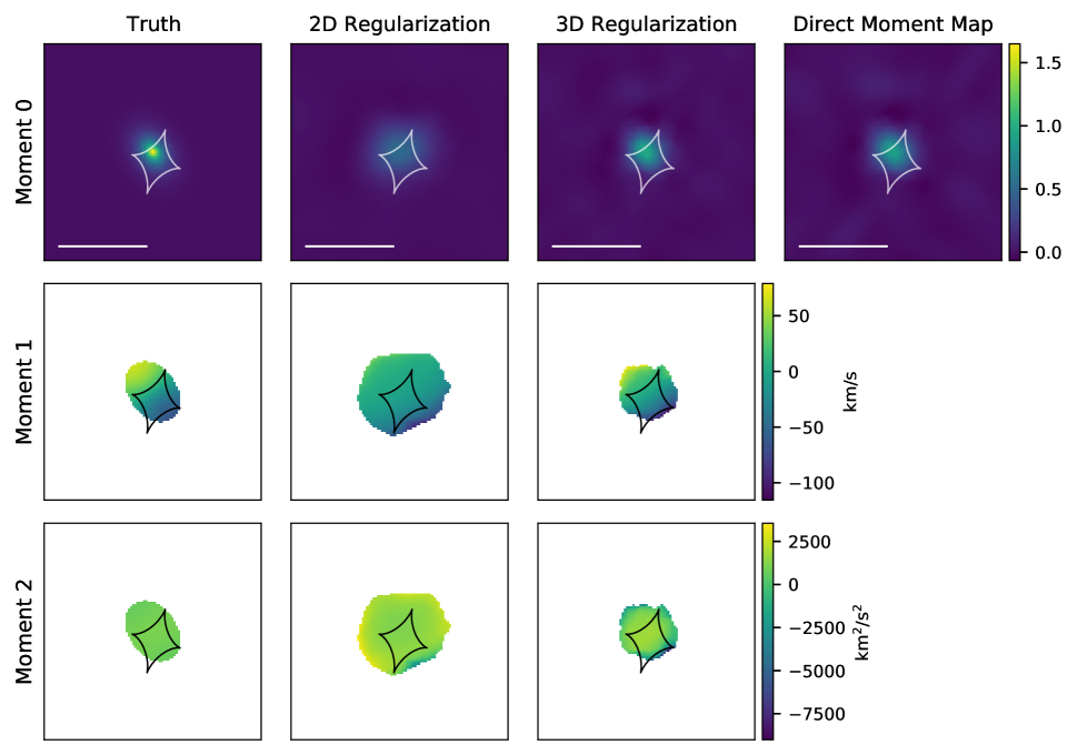
Figure 8: A comparison of the zeroth-, first-, and second-moment maps for the various reconstruction techniques. Columns, left to right: the “true” (input) source, the 2D-regularized reconstruction, the 3D-regularized reconstruction, and the reconstruction derived directly from the observed (lensed) moment map (see the text). Rows, top to bottom: the zeroth-, first-, and second-moment maps of the reconstructions. The first- and second-moment maps are shown with masks corresponding to $\textrm{S}/\textrm{N}\geq 3$ in the 2D and 3D zeroth-moment maps, while the truth mask shows pixels that are $\geq 1/2$ the peak surface brightness. The “direct” moment map does not have corresponding higher-order moments because it does not reconstruct the full source cube. The 3D zeroth-moment map reconstruction is similar in quality and effective resolution to the “direct” moment map reconstruction, while simultaneously recovering the full velocity structure of the cube. The greater compactness of the channel-by-channel 3D reconstruction allows it to better reproduce the velocity gradient of the true source compared to the 2D reconstruction.

We can also compare the various moment maps of the reconstructions to understand better how the full source intensity and velocity fields are reconstructed. Figure 8 shows the true source alongside the zeroth-moment maps derived from the 2D- and 3D-regularized reconstructions shown in Figure 3, as well as the reconstruction obtained from modeling the zeroth-moment map of the data directly. (We will refer to the latter as the “direct” zeroth-moment map reconstruction. Note that this reconstruction lacks all spectral information that was present in the data cube.) The 2D-regularized and “direct” moment maps differ because individual channels of the data cube have lower S/N than the zeroth-moment map. The lower S/N in the channels results in higher (per-channel) values of $\lambda$, and thus a lower effective resolution, compared to the single value of $\lambda$ used for the “direct” moment map reconstruction. Because of the different form of the regularization, the 3D source achieves an effective spatial resolution similar to that of the “direct” moment map reconstruction by fitting to the full cube simultaneously, while also reconstructing the entire velocity field of the source.

Comparing the higher-order moment maps in rows 2 and 3 of Figure 8, we can see that the 3D regularization reconstructs the first-moment map much better. This improvement occurs because the 2D regularization reproduces all of the channels less accurately (if at all). Most importantly, the first-moment calculation is sensitive to the emission in the outer channels where the 2D regularization performs the worst. We do not draw any conclusions from the comparison of the second-moment maps, due to the general difficulty of interpreting such higher moments in the presence of strong velocity gradients.

4.2.4 Spectral Resolution

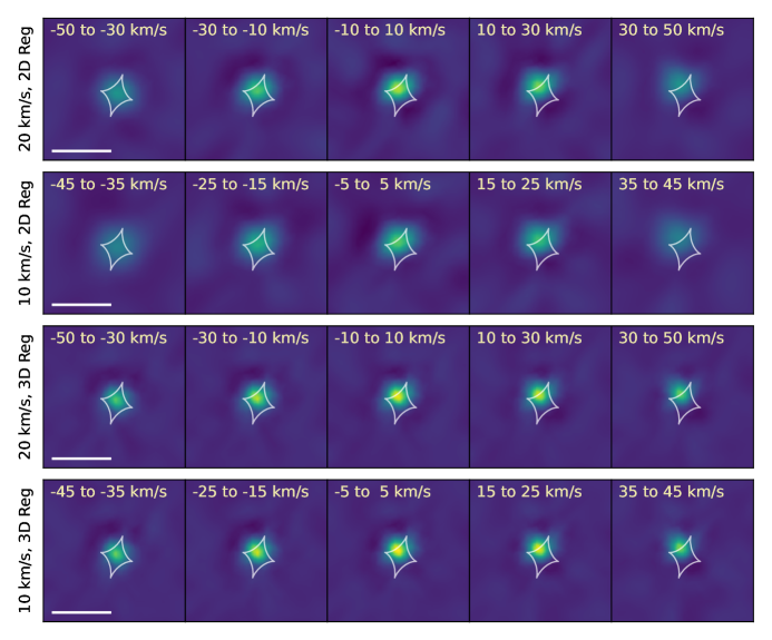
Figure 9: Select channel images using both reconstruction methods at two different spectral resolutions. The top two rows show $20$ and $10\,\text{km}\,\text{s}^{-1}$ resolutions, respectively, using 2D regularization, while the bottom two rows show the same for 3D regularization. Each panel gives the velocity range of the channel shown. Note that the two spectral resolutions have slightly different velocity ranges because of the alignment of the edges of the channels, but the channels are chosen and re-scaled to roughly match. Only a few channels near the line center are shown for clarity. Pixel values are in arbitrary integrated flux units. The top two rows show how the compactness of the 2D reconstructions is dependent on the channel width, while the bottom two rows show that the compactness of the 3D reconstructions is nearly independent of channel width.

To explore how the performance of the 3D regularization varies with spectral resolution, we simulate two versions of the fiducial set of observations with the same sensitivity but two different spectral resolutions of $10$ and $20\,\text{km}\,\text{s}^{-1}$. Figure 9 shows representative channel images of the difference between the truth and the reconstructions for the two mock cubes and for both regularization methods. The 2D reconstructions are sensitive to the choice of spectral resolution because narrower velocity channels result in channel images with lower S/Ns. Because the 3D regularization fits all channels together, it maintains a consistent source size and brightness profile regardless of the chosen channel width. This behavior is in line with the results of Chirivì et al. (2020), who find that their source parameter estimates are not negatively impacted (indeed, actually improve) as the number of channels increases, even as the per-channel S/N decreases.

4.2.5 Spatial Resolution

Figure 10: 2D- and 3D-regularized reconstructions for three different spatial resolutions. Rows, top to bottom: the zeroth-moment map of the mock data, the 2D-regularized reconstruction, and the 3D-regularized reconstruction. Columns, left to right: mock data with $0.25^{\prime\prime}$, $0.5^{\prime\prime}$, and $1^{\prime\prime}$ beams, respectively. The 3D reconstruction is consistently more compact at all spatial resolutions. The white bar shows $1^{\prime\prime}$.

We illustrate the trade-off between spatial and spectral resolutions in Figure 10, where we show the moment maps of reconstructions derived from three different sets of mock observations of the same source with $10\,\text{km}\,\text{s}^{-1}$ velocity bins and $0.25$, $0.5$, and $1^{\prime\prime}$ beams. Each of the data cubes has a peak S/N of 30. Both methods improve at higher spatial resolutions, but the 3D reconstruction is consistently more compact with a higher peak surface brightness, even achieving a size for a $0.5^{\prime\prime}$ beam comparable to that of the 2D source for a $0.25^{\prime\prime}$ beam. However, comparisons between spatial resolutions are complicated by the fact that the same S/N does not correspond to the same real-world exposure time at different resolutions.

The above comparison suggests that it may be more valuable in many cases to prioritize spectral resolution over spatial resolution to make the most effective use of available telescope time. Prospective users of multi-configuration interferometers like ALMA, for example, must often make difficult decisions about how to achieve compact synthesized beams $\sim\lambda/B_{\rm max}$: typical weather conditions limit the effective time available for observations at short wavelengths (i.e., small $\lambda$), especially when the array is in an extended configuration (i.e., the maximum projected baseline $B_{\rm max}$ is large). For a lensed source with a large velocity gradient, it may be easier to observe a longer-wavelength line in a more compact array configuration, as long as the S/N per channel does not become prohibitively low.

5 Conclusions

We have introduced modifications to a widely used Bayesian framework for reconstructing gravitationally lensed sources, to facilitate the modeling of sources observed with integral field spectroscopy. Because of the nature of integral field data, traditional (2D) regularization, which penalizes the squared gradient or Laplacian of each channel image independently, results in reconstructions that have lower effective resolutions and are unable to reproduce the full source velocity field accurately. Our newly introduced (3D) regularization scheme models the entire data cube simultaneously, instead penalizing the squared gradient or Laplacian of the entire 3D surface brightness distribution in order to account for the source velocity structure more effectively.

We have investigated the performance of the new method and the properties of the derived sources using simulated integral field observations of lensed rotating disks created using GalPaK${}^{\text{3D}}$ and lensmodel. We find that the 3D regularization leads to sources with higher effective resolutions and significantly better reconstructions in the faint, high-velocity outer channels as compared to the 2D approach. The resulting reconstructed 3D source cubes better reproduce both the zeroth- and first-moment maps of the data, in addition to the individual channel images.

The new form of the 3D regularization also changes the resolution and noise behavior in the source plane. Both the (spatially varying) noise and resolution structures of the resulting source are nearly constant across channel images in the 3D reconstruction compared to the spatial resolution and noise structure of the 2D reconstructions, which vary strongly across channels.

We find that — unlike the 2D reconstruction — the 3D reconstruction is robust to changes in the spectral resolution of the data. Along with the better accuracy of the reconstructed sources, this fact incentivizes obtaining higher spectral resolution observations of lensed sources even at the same cost to the per-channel S/N ratio of the data. Applying this new method to existing and future datasets will enable the extraction of more information about the kinematic properties of lensed sources and a better understanding of the underlying physics driving galaxies at high redshift.

Appendix A Including a Line-spread Function

For a single 2D image, the full lensing operator $\bm{L}$ is related to the blurring operator (the 2D PSF) $\bm{B}_{\rm P}$ and the lensing-only operator $\bm{L}^{\prime}$ via

$$\bm{L}=\bm{B}_{\rm P}\bm{L}^{\prime}.$$ (A1)

For data with no LSF, the 3D lensing matrix is given by

$$\bm{\hat{L}}\equiv\bm{I}_{N_{c}}\otimes\bm{L}.$$ (A2)

When the data have an LSF that spreads emission in the spectral direction, we can no longer write $\bm{\hat{L}}$ in block-diagonal form. Instead, we must rewrite $\bm{\hat{L}}$ in the more general form

$$\bm{\hat{L}}_{\rm LSF}=\bm{\hat{B}}_{\rm P,L}\bm{\hat{L}}^{\prime},$$ (A3)

where $\bm{\hat{L}}^{\prime}=\bm{I}_{\rm N_{\rm c}}\otimes\bm{L}^{\prime}$ is the lensing-only matrix for the 3D cube, and $\bm{\hat{B}}_{\rm P,L}$ computes the combined blurring of the entire cube by both the PSF and LSF.

$\bm{\hat{B}}_{\rm P,L}$ is a $N_{s}N_{c}\times N_{s}N_{c}$ block diagonal matrix. The blocks along the diagonal contain the 2D PSF. The off-diagonal blocks then show how a signal is spread into other channels; in general, blocks further from the diagonal will have lower amplitudes determined by the magnitude of the LSF for the given channel spacing.

Appendix B Derivation of the $\bm{\hat{Q}}$ Matrix

For a data cube with surface brightness distribution $\mathbf{S}(x,y,v_{z})$, the gradient and Laplacian can be written as

$$\nabla\mathbf{S}(x,y,v_{z})=\nabla_{x,y}\mathbf{S}(x,y,v_{z})+\nabla_{v_{z}}\mathbf{S}(x,y,v_{z}),$$ (B1)

and

$$\nabla^{2}\mathbf{S}(x,y,v_{z})=\nabla^{2}_{x,y}\mathbf{S}(x,y,v_{z})+\nabla^{2}_{v_{z}}\mathbf{S}(x,y,v_{z}),$$ (B2)

respectively. The $\nabla_{x,y}\mathbf{S}$ and $\nabla^{2}_{x,y}\mathbf{S}$ terms are computed by the (spatial) $\bm{H_{\text{2D}}}$ matrix, while the extra $\nabla_{v_{z}}\mathbf{S}$ and $\nabla^{2}_{v_{z}}\mathbf{S}$ terms are computed by the $\bm{\hat{Q}}$ matrix introduced in Section 2.2.1. Suyu et al. (2006) and Tagore & Keeton (2014) give the terms in $\bm{H_{\text{2D}}}$ for a regular and irregular grid, respectively.

Because the channel images (by assumption) have the same masks applied, the pixel grids for each channel are identical. Therefore, the $\nabla_{v_{z}}\mathbf{S}$ and $\nabla^{2}_{v_{z}}\mathbf{S}$ terms for a given pixel only depend on the corresponding pixels in adjacent channels. For a pixel $(i,j,k)$, where $i$ and $j$ denote the indices in the spatial directions and $k$ denotes the index for the spectral direction, we can compute the gradient and Laplacian using a central difference scheme. The gradient of the surface brightness is given by

$$\nabla_{v_{z}}\mathbf{S}(i,j,k)\propto\left[\mathbf{S}(i,j,k+1)-\mathbf{S}(i,j,k-1)\right]\hat{r}_{k-1,k},$$ (B3)

where $\hat{r}_{k-1,k}$ is the vector pointing from channel $k-1$ to channel $k$. The Laplacian is given by

$$\nabla^{2}_{v_{z}}\mathbf{S}(i,j,k)\propto\left[\mathbf{S}(i,j,k+1)+\mathbf{S}(i,j,k-1)-2\mathbf{S}(i,j,k)\right].$$ (B4)

Note that the proportionality constant in each relation is absorbed into the second regularization strength, $\eta$ (see Section 2.2.1).

We can adjust these terms for the edge channels by using a forward or backward difference instead of a central difference. The forward difference for the first derivative is given by

$$\nabla_{v_{z}}\mathbf{S}(i,j,k)\propto\left[\mathbf{S}(i,j,k+1)-\mathbf{S}(i,j,k)\right],$$ (B5)

and the backward difference is given by

$$\nabla_{v_{z}}\mathbf{S}(i,j,k)\propto\left[\mathbf{S}(i,j,k)-\mathbf{S}(i,j,k-1)\right].$$ (B6)

The forward difference for the second derivative is given by

$$\nabla^{2}_{v_{z}}\mathbf{S}(i,j,k)\propto\left[\mathbf{S}(i,j,k+2)-2\mathbf{S}(i,j,k+1)+\mathbf{S}(i,j,k)\right],$$ (B7)

and the backward difference is given by

$$\nabla^{2}_{v_{z}}\mathbf{S}(i,j,k)\propto\left[\mathbf{S}(i,j,k)-2\mathbf{S}(i,j,k-1)+\mathbf{S}(i,j,k-2)\right].$$ (B8)

Appendix C Resolution Analysis

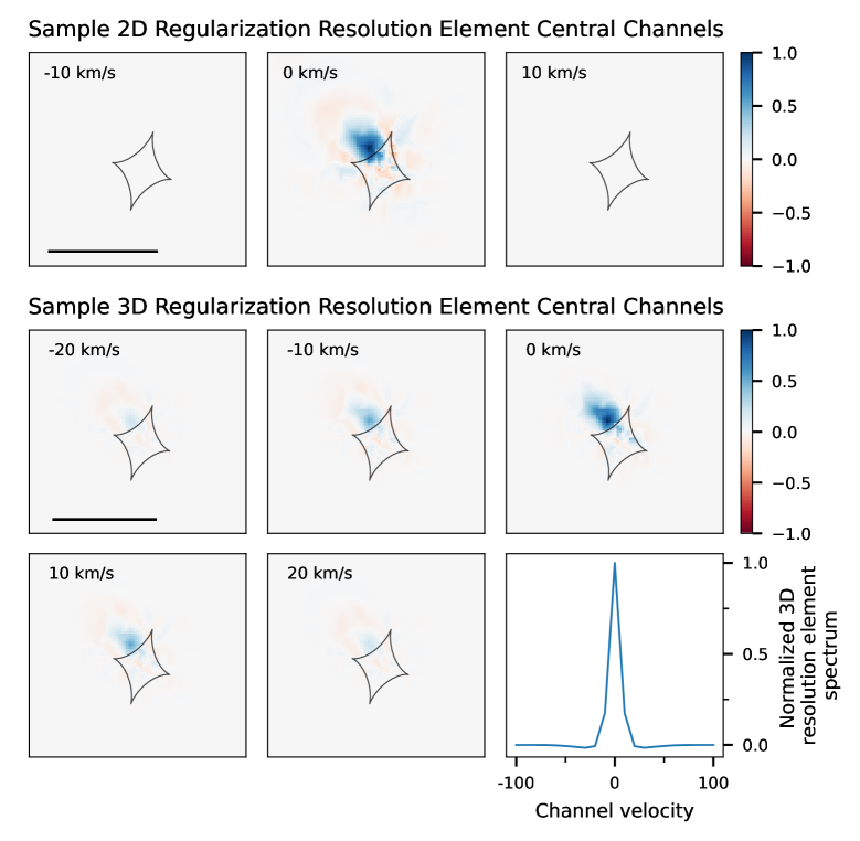
Figure 11: Example 3D effective resolution element in the source plane for each reconstruction method. Each beam corresponds to one column of the matrix $\bm{A}^{-1}\bm{F}$ in Equation C2. The top row shows the central three channels of the 2D effective resolution element. The resolution element only appears in the central channel because the reconstructed emission is not correlated between channels. The first five panels in the bottom two rows show the five central channels of the 3D effective resolution element, which contain most of the structure. The bottom right panel shows the spectrum of the 3D effective resolution element; here each channel is summed over the spatial pixels. Both resolution element cubes and the 3D beam spectrum are normalized to a peak of 1. Compared to the 2D case, the 3D resolution element shows less spatial “ringing,” particularly in the central channel. However, the 3D regularization creates correlations in the spectral direction that give the reconstruction of a point source an effective line width.

A number of considerations make quantifying the source-plane resolution difficult in general and even more difficult in the context of 3D regularization. First, regardless of the type of data, the variation of the magnification factor across the source plane gives rise to a resolution element that changes with position. Second, the reconstruction operation can also create ringing features (although regularization is designed to mitigate this) that result in highly non-Gaussian beams. Finally, the resolution element for the 3D regularization is three-dimensional because of the structure of the regularization matrix $\bm{\hat{R}_{\text{3D}}}$. Here we discuss some approaches to quantifying the resolution in the source plane and provide an example that illustrates the general behavior of the different resolution elements.

One approach to modeling beams in the source plane is to create mock observations with point sources, reconstruct those sources, and fit Gaussians to measure beam properties (e.g., Spilker et al., 2018). As an alternative that does not require extensive reconstructions with mock data, we can identify a matrix that describes the source-plane resolution elements. Consider starting with some source $\bm{s}_{0}$, creating a mock observation with noise, and then performing a reconstruction. The mock data can be written as $\bm{d}=\bm{L}\bm{s}_{0}+\bm{n}$ where $\bm{n}$ is a vector of noise in the data. Using Equations 4 and 8, we can write the reconstructed (most probable) source as

$$\bm{s}_{\text{MP}} =\bm{A}^{-1}\bm{L}^{\top}\bm{C}_{\textrm{d}}^{-1}\bm{d}$$

$$=\bm{A}^{-1}\bm{L}^{\top}\bm{C}_{\textrm{d}}^{-1}\bm{L}\bm{s}_{0}+\bm{A}^{-1}\bm{L}^{\top}\bm{C}_{\textrm{d}}^{-1}\bm{n}$$

$$=\bm{A}^{-1}\bm{F}\bm{s}_{0}+\bm{A}^{-1}\bm{L}^{\top}\bm{C}_{\textrm{d}}^{-1}\bm{n}.$$ (C1)

The reconstructed source is affected by the noise in the data. Averaging over many realizations of the noise,

$$\langle\bm{s}_{\text{MP}}\rangle =\langle\bm{A}^{-1}\bm{F}\bm{s}_{0}\rangle+\langle\bm{A}^{-1}\bm{L}^{\top}\bm{C}_{\textrm{d}}^{-1}\bm{n}\rangle$$

$$=\bm{A}^{-1}\bm{F}\bm{s}_{0}.$$ (C2)

The first term is independent of noise, and the last term vanishes because $\langle\bm{M}\bm{n}\rangle=0$ for any linear operator $\bm{M}$. The matrix $\bm{A}^{-1}\bm{F}$ thus represents the combined actions of lensing and computing the noise-averaged reconstruction $\langle\bm{s}_{\text{MP}}\rangle$ for a given source $\bm{s}_{0}$. If we let $\bm{s}_{0}$ represent individual source pixels, we can see that the columns of $\bm{A}^{-1}\bm{F}$ give the noise-averaged reconstructions of a set of point sources located at the vertices of the source-plane grid. These column vectors are the effective resolution elements in the source plane. This argument holds for the 3D case as well if the matrices are replaced by their hatted counterparts.

For 2D regularization $\bm{\hat{A}}^{-1}\bm{\hat{F}}$ is block-diagonal, so each resolution element is confined to only one channel. However, 3D regularization produces entries in the off-diagonal blocks of $\bm{\hat{A}}^{-1}\bm{\hat{F}}$ that manifest as components of the resolution element in neighboring channels. The differences between the 2D and 3D resolution elements can be seen in Figure 11, which shows examples appropriate for a position near the caustic that is centered on the central channel of the cube.

The 2D regularization resolution element shown in Figure 11 is for the central (highest S/N) channel of the source plane cube. The comparison of this channel resolution element to the 3D regularization resolution element is the most favorable for the 2D regularization, since the 2D resolution elements become significantly larger at velocities farther from systemic, due to their lower S/N. The higher spatial resolution of the 3D regularization across all of the channels appears to be the driver of the better source reconstruction shown in Figure 3. The 3D regularization resolution element shows reduced spatial ringing in the central channel, but also shows emission spread into neighboring channels. In this case, most of the emission is confined to the central five channels ($50\,\text{km}\,\text{s}^{-1}$). The spectral width of the 3D regularization resolution element depends on the spectral regularization strength $\eta$.

References

- Astropy Collaboration et al. (2013) Astropy Collaboration, Robitaille, T. P., Tollerud, E. J., et al. 2013, A&A, 558, A33
- Astropy Collaboration et al. (2018) Astropy Collaboration, Price-Whelan, A. M., Sipőcz, B. M., et al. 2018, AJ, 156, 123
- Birrer et al. (2015) Birrer, S., Amara, A., & Refregier, A. 2015, The Astrophysical Journal, 813, 102
- Bouché et al. (2015) Bouché, N., Carfantan, H., Schroetter, I., Michel-Dansac, L., & Contini, T. 2015, The Astronomical Journal, 150, 92
- Brewer & Lewis (2006) Brewer, B. J., & Lewis, G. F. 2006, The Astrophysical Journal, 637, 608
- Chen et al. (2008) Chen, Y., Davis, T. A., Hager, W. W., & Rajamanickam, S. 2008, ACM Trans. Math. Softw., 35, doi:10.1145/1391989.1391995
- Chirivì et al. (2020) Chirivì, G., Yıldırım, A., Suyu, S. H., & Halkola, A. 2020, A&A, 643, A135
- Cresci et al. (2010) Cresci, G., Mannucci, F., Maiolino, R., et al. 2010, Nature, 467, 811
- Dye & Warren (2005) Dye, S., & Warren, S. J. 2005, The Astrophysical Journal, 623, 31
- Geach et al. (2018) Geach, J. E., Ivison, R. J., Dye, S., & Oteo, I. 2018, The Astrophysical Journal Letters, 866, L12
- Genzel et al. (2017) Genzel, R., Förster Schreiber, N. M., Übler, H., et al. 2017, Nature, 543, 397
- Genzel et al. (2020) Genzel, R., Price, S. H., Übler, H., et al. 2020, ApJ, 902, 98
- Harris et al. (2020) Harris, C. R., Millman, K. J., van der Walt, S. J., et al. 2020, Nature, 585, 357
- Hezaveh et al. (2017) Hezaveh, Y. D., Perreault Levasseur, L., & Marshall, P. J. 2017, Nature, 548, 555
- Hunter (2007) Hunter, J. D. 2007, Computing in Science & Engineering, 9, 90
- Jones et al. (2010) Jones, T. A., Swinbank, A. M., Ellis, R. S., Richard, J., & Stark, D. P. 2010, MNRAS, 404, 1247
- Keeton (2011) Keeton, C. R. 2011, GRAVLENS: Computational Methods for Gravitational Lensing, ascl:1102.003
- Kochanek & Narayan (1992) Kochanek, C., & Narayan, R. 1992, The Astrophysical Journal, 401, 461
- Morningstar et al. (2019) Morningstar, W. R., Perreault Levasseur, L., Hezaveh, Y. D., et al. 2019, ApJ, 883, 14
- Patrício et al. (2018) Patrício, V., Richard, J., Carton, D., et al. 2018, Monthly Notices of the Royal Astronomical Society, 477, 18
- Perreault Levasseur et al. (2017) Perreault Levasseur, L., Hezaveh, Y. D., & Wechsler, R. H. 2017, ApJ, 850, L7
- Refregier (2003) Refregier, A. 2003, MNRAS, 338, 35
- Riechers et al. (2008) Riechers, D. A., Walter, F., Brewer, B. J., et al. 2008, ApJ, 686, 851
- Rizzo et al. (2018) Rizzo, F., Vegetti, S., Fraternali, F., & Di Teodoro, E. 2018, Monthly Notices of the Royal Astronomical Society, 481, 5606
- Rizzo et al. (2021) Rizzo, F., Vegetti, S., Fraternali, F., Stacey, H. R., & Powell, D. 2021, MNRAS, 507, 3952
- Scoville et al. (1997) Scoville, N. Z., Yun, M. S., & Bryant, P. M. 1997, ApJ, 484, 702
- Sharon et al. (2019) Sharon, C. E., Tagore, A. S., Baker, A. J., et al. 2019, The Astrophysical Journal, 879, 52
- Spilker et al. (2018) Spilker, J. S., Aravena, M., Béthermin, M., et al. 2018, Science, 361, 1016
- Stark et al. (2008) Stark, D. P., Swinbank, A. M., Ellis, R. S., et al. 2008, Nature, 455, 775
- Suyu et al. (2006) Suyu, S. H., Marshall, P. J., Hobson, M. P., & Blandford, R. D. 2006, Monthly Notices of the Royal Astronomical Society, 371, 983
- Tagore & Jackson (2016) Tagore, A. S., & Jackson, N. 2016, Monthly Notices of the Royal Astronomical Society, 457, 3066
- Tagore & Keeton (2014) Tagore, A. S., & Keeton, C. R. 2014, Monthly Notices of the Royal Astronomical Society, 445, 694
- Tikhonov et al. (1995) Tikhonov, A. N., Goncharsky, A., Stepanov, V. V., & Yagola, A. G. 1995, Numerical Methods for the Solution of Ill-Posed Problems (Springer, Dordrecht)
- Vegetti & Koopmans (2009) Vegetti, S., & Koopmans, L. V. E. 2009, MNRAS, 392, 945
- Virtanen et al. (2020) Virtanen, P., Gommers, R., Oliphant, T. E., et al. 2020, Nature Methods, 17, 261
- Wallington et al. (1996) Wallington, S., Kochanek, C. S., & Narayan, R. 1996, ApJ, 465, 64
- Warren & Dye (2003) Warren, S. J., & Dye, S. 2003, The Astrophysical Journal, 590, 673