Machine Learning Wavefunction

Abstract

This chapter introduces the main ideas and the most important methods for representing the electronic wavefunction through machine learning models. The wavefunction of a $N$-electron system is an incredibly complicated mathematical object, and models thereof require enough flexibility to properly describe the complex interactions between the particles, but at the same time a sufficiently compact representation to be useful in practice. Machine learning techniques offer an ideal mathematical framework to satisfy these requirements, and provide algorithms for their optimization in both supervised and unsupervised fashions. In this chapter, various examples of machine learning wavefunctions are presented and their strengths and weaknesses with respect to traditional quantum chemical approaches are discussed; first in theory, and then in practice with two case studies.

1 Introduction

We shall start this chapter by introducing the mathematical infrastructure in which wavefunction methods are defined, and then provide a brief overview of the machine learning (ML) approaches that have been developed within this framework. This will set the stage for the remainder of this chapter, where we will discuss in more detail a number of methods that successfully leverage ML techniques to represent the electronic wavefunction.

At the heart of wavefunction theory and the electronic structure problem lies the time-independent Schrödinger equation (TISE)

$$\hat{H}\Psi=E\Psi$$ (1)

where $\Psi$ is the wavefunction describing the quantum state, $E$ is its associated energy, and $\hat{H}$ is the ab initio electronic Hamiltonian. The latter is given (in atomic units) by

$$\hat{H}=-\sum_{i=1}^{N}\frac{1}{2}\nabla_{i}-\sum_{i=1}^{N}\sum_{I=1}^{N_{atoms}}\frac{Z_{I}}{|\mathbf{r}_{i}-\mathbf{R}_{I}|}+\sum_{i=1}^{N}\sum_{j>i}^{N}\frac{1}{|\mathbf{r}_{i}-\mathbf{r}_{j}|}+\sum_{I=1}^{N_{atoms}}\sum_{J>I}^{N_{atoms}}\frac{Z_{I}Z_{J}}{|\mathbf{R}_{I}-\mathbf{R}_{J}|}$$ (2)

with the first term describing the kinetic energy of the electrons, the second term the attraction between electrons and nuclei, and the third and fourth terms the electron-electron and nuclear-nuclear repulsion, respectively. Within the Born–Oppenheimer approximation, the wavefunction $\Psi$ only depends on the position $\mathbf{r}=(\mathbf{r}_{1},\ldots,\mathbf{r}_{N})$ of the $N$ electrons

$$\Psi\equiv\Psi(\mathbf{r}_{1},\ldots,\mathbf{r}_{N})=\Psi(\mathbf{r})$$ (3)

and encodes all the information of the $N$-particle system. This mathematical object is incredibly complex and constitutes the quantity subject to approximations in wavefunction theory. Typically, the first step in the practical resolution of Equation 1 is the introduction of a finite many-particle basis, $\{\Phi_{I}\}_{I=0}^{M}$, and the expansion of the wavefunction $\Psi$ in this basis. We thus have the following ansatz

$$\Psi(\mathbf{r}_{1},\ldots,\mathbf{r}_{N})=\sum_{I=0}^{M}C_{I}\Phi_{I}(\mathbf{r}_{1},\ldots,\mathbf{r}_{N})$$ (4)

where the coefficients $C_{I}$ are a priori unknown parameters (forming a vector $\mathbf{C}$), that can be determined by minimizing the energy expectation value according to the variational principle

$$\mathbf{C}^{*}=\operatorname*{argmin}_{\mathbf{C}}\frac{\braket{\Psi}{\hat{H}}{\Psi}}{\braket{\Psi}{\Psi}}$$ (5)

Not any type of many-particle function $\Phi_{I}$ can be used in Equation 4, because a fermionic wavefunction has to be antisymmetric with respect to the permutations of two identical particles, i.e.

$$\Psi(\mathbf{r}_{1},\ldots,\mathbf{r}_{i},\mathbf{r}_{j},\ldots,\mathbf{r}_{N})=-\Psi(\mathbf{r}_{1},\ldots,\mathbf{r}_{j},\mathbf{r}_{i},\ldots,\mathbf{r}_{N})$$ (6)

The most common and practical choice to explicitly enforce this property is to choose Slater determinants (SDs) as the many-particle functions $\Phi_{I}$, which are constructed from a finite one-electron basis $\{\phi_{i}\}_{i=1}^{m}$. Importantly, the introduction of this orbital basis allows us to express Equation 4 as a linear combination of occupation number vectors in Fock space

$$\ket{\Psi}=\sum_{\sigma_{1},\sigma_{2},\ldots,\sigma_{m}}\psi_{\sigma_{1},\sigma_{2},\ldots,\sigma_{m}}\ket{\sigma_{1},\sigma_{2},\ldots,\sigma_{m}}=\sum_{\bm{\sigma}}\psi_{\bm{\sigma}}\ket{\bm{\sigma}}$$ (7)

where $\sigma_{i}=0$ if the spin-orbital $\phi_{i}$ is empty and $\sigma_{i}=1$ if it is occupied (note that it is also common to use molecular orbitals, in which case we would have 4 possible states: $\sigma_{i}\in\{\cdot,\uparrow,\downarrow,\mathbin{\uparrow}\downarrow\}$). In this representation, a Slater determinant $\Phi_{I}$ is encoded by the occupation pattern of the orbitals, and the amplitudes $\psi_{\bm{\sigma}}$ parametrizing the wavefunction, are labeled by the corresponding many-body configuration $\bm{\sigma}=(\sigma_{1},\sigma_{2},\ldots,\sigma_{m})$. Note that the amplitudes $\psi_{\bm{\sigma}}$ in Equation 7 are nothing but a relabeling of the coefficients $C_{I}$ of Equation 4. One advantage of Equation 7 is that it also naturally represents quantum states of model Hamiltonians that are defined on discrete lattices, see Figure 1 for the comparison of a Slater determinant and a lattice. These are the systems targeted by the first machine learning approaches that we will see in the next section, thus it is important to draw the connection between them and the language of quantum chemists.

Figure 1: Graphical representation of a Slater determinant (left) and of a 1D lattice (right). The occupation numbers $\sigma_{i}$ refer to molecular orbitals for the SD, and to individual spins on lattice sites for the 1D lattice.

When the many-body configurations in Equation 7 represent Slater determinants, the ansatz is called full configuration interaction (FCI). Within a given one-particle basis, the FCI method yields the exact solution of Equation 1, however it is only applicable to few-particle systems due to its unfavorable computational scaling. In fact, the FCI ansatz highlights one major challenge intrinsic to the quantum many-body problem, that is, the size of the space of many-body configurations in which the solution $\Psi$ of Equation 1 lives in, grows exponentially with the number of particles $N$ (or, equivalently, the number of one-particle basis functions $m$). This is manifestly visible in Equation 7, where the sum runs over all possible $2^{m}$ many-body configurations. A major goal of electronic structure theory is to find approximations to Equation 7 that only contain a polynomial number of parameters, yet capturing the most important correlation features by retaining only the dominant configurations. To this end, many approximate wave function ansätze have been proposed throughout the years. Historically, the predominant recipe to approximate wavefunctions has been to truncate the sum in Equation 7 according to the number of excitations from a reference SD (or several reference SDs), resulting in a series of systematically improvable ansätze. These are for example the configuration interaction, coupled cluster and perturbation theory approaches discussed briefly in chapter 1. More recently, alternative parametrizations stemming from the condensed matter physics community have emerged, such as matrix product states, where the idea is to fix a maximum number of many-particle functions, but allow them to change iteratively in an algorithm known as the density matrix renormalization group [1]. If only a single many-particle basis function is retained in the ansatz of Equation 4, we recover the Hartree-Fock approximation, a cornerstone of electronic structure theory since its inception. From this discussion, it is clear that the FCI ansatz offers the greatest flexibility, however it is computationally untractable due to its exponential scaling. On the other end of the spectrum, the HF approximation is the most compact, but its accuracy is not sufficient for most applications. We need to find the right compromise between these two extremes; this is the entry point for machine learning approaches.

The astonishing success that machine learning is having in representing high-dimensional data with complex dependencies offers new avenues for the electronic structure problem. In fact, machine learning techniques to solve the Schrödinger equation were already explored more than a decade ago [2, 3, 4, 5], despite passing relatively unnoticed. It is only thanks to the current success that ML is having in other fields of computational chemistry and physics, that the interest to apply it to wavefunction theory has resurged as well. There are several ways to harness the power and flexibility of machine learning in the context of wavefunction theory. One possibility is to use them to improve or accelerate existing methods, such as in the machine learning configuration interaction approach by [6] or the accelerated coupled cluster by [7]. These ideas and their implementation details were the subject of chapter 22 and will not be discussed further here. Instead, the main topic for the remainder of this chapter are ML models that are directly used to represent the wavefunction. These try to completely bypass the standard framework of expressing an analytically integrable ansatz (typically based on Gaussian orbitals), and obtain the optimal parameters through the solution of an eigenvalue equation or many-body conditions. In this respect, the very first work in recent times that showed the true power and flexibility of ML approaches to solve the Schrödinger equation is that by [8]. Here, the authors proposed a particular type of neural network (NN) — the restricted Boltzmann machine (RBM) — that was able to encode the ground state of two paradigmatic spin Hamiltonians with state-of-the-art accuracy. The exceptional result of this neural-network quantum state (NQS) ansatz led to a large number of follow-up works within the condensed matter physics community. For instance, the relation of RBMs to the more known tensor network states was quickly made [9, 10, 11, 12, 13] and their characterization in terms of quantum entanglement [14] and representability theorems [15] was established. It was shown how to include abelian and non-abelian symmetries in the ansatz [16, 17], meanwhile many extensions of, and alternatives to, the simple RBM architecture to more general NNs were developed, resulting in new NQS ansätze [18, 19, 20, 21, 22, 23, 24, 25]. The application of restricted Boltzmann machines to solve the TISE with the full ab initio electronic Hamiltonian was also shown possible. In a few cases, the electronic structure problem was mapped from fermionic degrees of freedom to spin ones, and essentially the same technique as used in the original work by [8] was then used to obtain the ground state energy of several small molecular systems and the dissociation curves of a few diatomic molecules [19, 26]. The accuracy reached in this case was on-par or beyond that of CCSD(T), albeit only in conjunction with a minimal basis set. Neural-network quantum states have also seen application as active space solvers in the context of the CASSCF method, with promising results [27]. A significant step forward was made with the development of two similar ansätze based on deep neural networks (DNNs). The FermiNet [28] and PauliNet [29] architectures completely bypass the typical dependence on a one-electron basis set and directly represent the wavefunction in real space. While an earlier attempt based on DNNs did not consistently reach an acceptable accuracy [30], both FermiNet and PauliNet yielded results comparable or superior to the best methods currently available across the board. All the ML-based wavefunctions mentioned so far are true ab initio ansätze in the sense that do not require prior data to be trained, rather their parameters are optimized in an unsupervised fashion. On the other hand, supervised techniques are also possible. Examples of these have been already discussed in chapter 18 in the context of DFT, where for instance, the electronic density was learned from reference data and predicted by Gaussian process regression [31] or neural networks [32]. In the same spirit, but in the framework of wavefunction theory, the SchNOrb deep convolutional neural network predicts the electronic wavefunction by learning the Hamiltonian and overlap matrices expressed in the molecular orbital basis from a set of reference calculations [33, 34].
At last, while neural networks have been clearly the favorite choice so far, recent works exploring the efficacy of Gaussian processes to represent the wavefunction have shown that non-parametric approaches are equally valid alternatives [35, 36]. In fact, the so-called Gaussian process state (GPS) is able to reach and surpass the accuracy of RBMs in the solution of the Fermi-Hubbard model, with a very compact representation of the ground state wavefunction.

In the next section we shall discuss in more detail a number of different ML approaches to the solution of the Schrödinger equation and place them in the larger context of electronic structure theory. We shall analyze strengths and weaknesses of these methods and see how they compare to their traditional counterparts. Finally, you will have the chance to get first-hand experience with these new powerful tools through two case studies.

2 Methods

The discussion of this section is divided based on the (mathematical) space in which the methods are defined. First, we look at approaches expressed in the Fock space of many-body configurations, as these are conceptually closer to the usual framework used in traditional quantum chemical methods. Second, we consider ansätze in first quantization, that is, defined directly in the real space of electronic coordinates. The third subsection is devoted to a supervised method that is neither defined in Fock space, nor in real space. Instead, it infers the wavefunction of a system directly from the molecular geometry. However, before dwelling into the discussion of these methodologies, we shall go through a short introduction to variational Monte Carlo (VMC), as this technique is a common denominator for the complicated ansätze considered here.

2.1 Variational Monte Carlo in a nutshell

The underlying idea of variational Monte Carlo is to evaluate the high-dimensional integrals appearing in the quantum many-body problem by the Monte Carlo method [37]. Consider the energy expectation value $E$ associated to the quantum state $\Psi$,

$$E=\frac{\braket{\Psi}{\hat{H}}{\Psi}}{\braket{\Psi}{\Psi}}=\frac{\int\Psi^{*}(\mathbf{r})\hat{H}\Psi(\mathbf{r})\mathrm{d}\mathbf{r}}{\int\Psi^{*}(\mathbf{r})\Psi(\mathbf{r})\mathrm{d}\mathbf{r}}$$ (8)

The right-hand side contains integrals over the whole $3N$-dimensional space which are hard to evaluate numerically. However, the integrands can be manipulated into more a convenient expression which is amenable for the Monte Carlo technique. That is,

$$\frac{\int\Psi^{*}(\mathbf{r})\hat{H}\Psi(\mathbf{r})\mathrm{d}\mathbf{r}}{\int\Psi^{*}(\mathbf{r})\Psi(\mathbf{r})\mathrm{d}\mathbf{r}}=\frac{\int|\Psi(\mathbf{r})|^{2}\tfrac{\hat{H}\Psi(\mathbf{r})}{\Psi(\mathbf{r})}\mathrm{d}\mathbf{r}}{\int|\Psi(\mathbf{r})|^{2}\mathrm{d}\mathbf{r}}=\int\frac{|\Psi(\mathbf{r})|^{2}}{\int|\Psi(\mathbf{r})|^{2}\mathrm{d}\mathbf{r}}\frac{\hat{H}\Psi(\mathbf{r})}{\Psi(\mathbf{r})}\mathrm{d}\mathbf{r}=\int\rho(\mathbf{r})E_{loc}(\mathbf{r})\mathrm{d}\mathbf{r}$$ (9)

where $\rho(\mathbf{r})$ is interpreted as a probability distribution and $E_{loc}(\mathbf{r})=\tfrac{\hat{H}\Psi(\mathbf{r})}{\Psi(\mathbf{r})}$ is the so-called local energy. By drawing a finite number $N_{s}$ of sample points $\{\mathbf{r}^{(k)}\}_{k=1}^{N_{s}}$ according to $\rho(\mathbf{r})$, the energy expectation value can be approximated as an average over local energies as

$$E\approx\frac{1}{N_{s}}\sum_{k=1}^{N_{s}}E_{loc}(\mathbf{r}^{(k)})$$ (10)

A typical choice to sample the points $\{\mathbf{r}^{(k)}\}_{k=1}^{N_{s}}$ is to walk in $3N$-dimensional space and generate a Markov chain of electronic coordinates, $\mathbf{r}^{(1)}\to\mathbf{r}^{(2)}\to\ldots\to\mathbf{r}^{(N_{s})}$, through the Metropolis-Hastings algorithm [38, 39]. This is an efficient way to generate the new positions, because the usually complicated integral in the denominator of $\rho(\mathbf{r})$ does not need to be evaluated. The traditional wavefunction ansatz used in VMC (also called trial wavefunction within the quantum Monte Carlo community) is of the Slater-Jastrow type [40], and has the following general form

$$\Psi_{\bm{\Theta}}(\mathbf{r})=\mathcal{J}(\mathbf{r},\bm{\Theta})\Phi_{0}(\mathbf{r})$$ (11)

Here, $\Phi_{0}(\mathbf{r})$ is a mean-field solution (such as the Hartree-Fock determinant) or a small linear combination of SDs, while $\mathcal{J}(\mathbf{r},\bm{\Theta})$ is a Jastrow factor which depends on a set of variational parameters $\bm{\Theta}$. In $\Psi_{\bm{\Theta}}(\mathbf{r})$, the Jastrow factor captures short-range electron correlation effects, and because the integrals in Equation 8 are not evaluated directly, $\mathcal{J}(\mathbf{r},\bm{\Theta})$ admits very complicated functional forms that typically depend on the inter-electronic distances explicitly. The mean-field component on the other hand, fixes the nodal structure of the wavefunction, such that the accuracy of any VMC calculation is ultimately dictated by $\Phi_{0}(\mathbf{r})$, regardless of the choice of the Jastrow factor. A possible way to improve this situation is to use a backflow transformation [41], which modifies the coordinates of each electron in $\Phi_{0}(\mathbf{r})$ based on the position of all the others

$$\mathbf{r}_{i}\to\mathbf{x}_{i}=\mathbf{r}_{i}+\bm{\xi}_{i}(\mathbf{r})$$ (12)

thus moving the position of the nodes. For electronic problems in real space, the Slater-Jastrow-backflow form is currently the default choice. However, we shall see later on in this chapter how neural networks can improve upon it. To obtain the best possible energy $E$ with the ansatz $\Psi_{\bm{\Theta}}(\mathbf{r})$, the expectation value of Equation 8 is minimized with respect to the variational parameters $\bm{\Theta}$. This is done by starting from an initial set $\bm{\Theta}^{(0)}$, which is updated in an iterative fashion. At iteration $t$, the new parameters for $t+1$ are obtained with

$$\bm{\Theta}^{(t+1)}=\bm{\Theta}^{(t)}-\mathcal{F}(\bm{\Theta}^{(t)})$$ (13)

where the function $\mathcal{F}(\bm{\Theta})$ takes different forms depending on the particular numerical technique chosen. The simplest option, which is also widely used in the machine learning community, is gradient descent and its stochastic version. In this case, the parameters are optimized by taking steps along the direction pointed by the negative of the energy gradient

$$\bm{\Theta}^{(t+1)}=\bm{\Theta}^{(t)}-\alpha\nabla_{\bm{\Theta}}E(\bm{\Theta}^{(t)})$$ (14)

where $\alpha$ is a scalar value determining the step size. In practice, a first-order scheme such as gradient descent, while computationally cheap, might require hundreds of iterations to reach convergence. A more robust option typically used in VMC is the stochastic reconfiguration (SR) approach by [42], however its details are beyond the scope of this introduction, hence they will not be discussed here.

To summarize, a VMC calculation consists in the following steps:

1. Obtain $\Phi_{0}$ and apply the backflow transformation to the electronic coordinates

2. Initialize randomly the Jastrow factor parameters to $\bm{\Theta}^{(0)}$

3. Perform a Monte Carlo sweep and sample $N_{s}$ positions through the Metropolis-Hastings algorithm

4. Compute the energy expectation value according to Equation 10

5. Check if the energy is converged (or a predefined maximum of MC sweeps is reached)

6. Terminate the calculation if converged, otherwise continue to the next step

7. Compute the gradients, update the parameters with Equation 13 and go back to step 3.

The major advantage of VMC over other techniques is that it circumvents the analytical integration of Equation 8, allowing for the very expressive and complicated wavefunction ansätze based in machine learning models, e.g. neural networks. At last, we should note that even though we have presented VMC as a real space approach, the same technique can be used to optimize wavefunctions defined in any other space, such as that of many-body configurations.

2.2 Modeling the wavefunction in Fock space

We have seen in the beginning of this chapter that the first step for the practical resolution of Equation 1 is the introduction of a finite basis of many-body configurations, Equation 7. It is not surprising then, that the first major successful attempts to encode the wavefunction using a ML-inspired approach were obtained in this framework. In fact, working in Fock space presents several advantages, for instance in the interpretation of the correlation features and the physics underpinning the studied systems. After all, this is the basis in which most of the modern computational quantum physics and chemistry has been developed, such that we have come a long way in interpreting and analyzing results in these terms. In the following we shall discuss two unsupervised approaches to the solution of the Schrödinger equation, one based on a parametric model — the neural-network quantum state ansatz — and one based on a non-parametric one — the Gaussian process state ansatz.

2.2.1 Neural-network quantum state

The main idea behind the neural-network quantum state ansatz is to use a neural network to represent the wavefunction. There are many types of network architectures that can be used for this purpose, however, here we will focus on the most famous one introduced by [8], the restricted Boltzmann machine, and only briefly discuss possible extensions and alternatives.

Restricted Boltzmann machines.
A restricted Boltzmann machine is a generative model originally developed to represent classical probability functions, and that can be used to generate new samples according to the distribution learned from the underlying data. This is achieved by defining an energy function

$$E(\mathbf{v},\mathbf{h})=-\sum_{j=1}^{m}a_{j}v_{j}-\sum_{i=1}^{n}b_{i}h_{i}-\sum_{i=1}^{n}\sum_{j=1}^{m}h_{i}W_{ij}v_{j}$$ (15)

which depends on interconnected visible and hidden binary variables $v_{j},h_{i}\in\{-1,1\}$, respectively. Their joint probability density $p(\mathbf{v},\mathbf{h})$ is assumed to follow the Boltzmann distribution

$$p(\mathbf{v},\mathbf{h})=\frac{1}{Z}e^{-E(\mathbf{v},\mathbf{h})}$$ (16)

where $Z$ is the partition function defined in the same way as in statistical physics, ensuring that the probabilities sum up to one. The crucial breakthrough has been to interpret the marginal distribution over the visible units as wavefunction amplitudes, that is

$$p(\mathbf{v})=\sum_{\mathbf{h}}p(\mathbf{v},\mathbf{h})=\psi(\mathbf{v})$$ (17)

In this context, the vector $\mathbf{v}$ of visible units represents a many-body configuration $\bm{\sigma}$, whose correlation is mediated by the hidden variables $\{h_{i}\}_{i=1}^{m}$. This architecture, shown in Figure 2, results in the following ansatz for the wavefunction amplitudes (note the switch in notation from $\mathbf{v}$ to $\bm{\sigma}$ for the input vector)

$$\psi(\bm{\sigma})=\sum_{\mathbf{h}}e^{\sum_{j}a_{j}\sigma_{j}+\sum_{i}b_{i}h_{i}+\sum_{i,j}h_{i}W_{ij}\sigma_{j}}$$ (18)

where, without loss of generality, the normalization factor $Z^{-1}$ from Equation 16 was dropped for simplicity.

Figure 2: The RBM network architecture underpinning the NQS ansatz introduced by [8]. The weights between the hidden and outputs layers are fixed to unity, and simply act as a sum.

Thanks to the fact that there is no intralayer connection among the hidden units, the external sum in Equation 18 can be analytically traced out, yielding the expression

$$\psi(\bm{\sigma})=\prod_{j=1}^{m}e^{a_{j}\sigma_{j}}+\prod_{i=1}^{n}2\cosh\Big{(}b_{i}+\sum_{j=1}^{m}W_{ij}\sigma_{j}\Big{)}$$ (19)

which can be efficiently evaluated for each $\bm{\sigma}$. Equations 18 and 19 are manifestly non-negative. This is a necessary requirement for modeling probability distributions, however, in the context of fermionic wavefunctions, constitutes a shortcoming. Indeed, for a complete description of a quantum state, both the amplitude and the phase factor of the wavefunction are needed, such that in practice, the network weights are required to admit complex numbers. This is the approach used in the original work [8], however extensions to more complicated architectures explicitly encoding the sign of the amplitude [19, 21] or based on deep Boltzmann machines are also possible [20, 27], allowing the weights to remain real numbers.
From a physics standpoint, we can understand the neural network of Figure 2 by thinking of the particle(s) sitting on the local state $\sigma_{j}$ as interacting with the ones described by $\sigma_{k\neq j}$ through the auxiliary degrees of freedom provided by the hidden units $h_{i}$. In this framework, the weights $\mathbf{W}$ and bias vectors $\mathbf{a}$ and $\mathbf{b}$ regulate the magnitude of these interactions, effectively encoding correlation between the particles. By increasing the number $n$ of hidden units, or equivalently the hidden-unit density $\alpha=\tfrac{n}{m}$, the wavefunction becomes more expressive and can describe higher-order correlation features. Importantly, while the number of possible Fock space configurations increases exponentially with the system size $m$, the number of parameters defining the RBM only grows as $\mathcal{O}(nm+n+m)$. The ability to predict the amplitude $\psi(\bm{\sigma})$ of exponentially many configurations $\bm{\sigma}$, with a parametrization that only scales polynomially, is one of the key features underlying the RBM ansatz. Ultimately, the accuracy is dictated by the density $\alpha$, and in principle, there is no upper limit to the width of the hidden layer. In fact, RBMs are known as universal approximators [43], capable to reproduce any probability distribution to arbitrary accuracy, provided enough hidden units are included.
It is important to realize that the parametrization achieved through Equation 19 does not represent a wavefunction expressed in an actual many-particle basis. Instead, it just encodes the amplitudes $\psi_{\bm{\sigma}}=\psi_{RBM}(\bm{\sigma})$ of the expansion given in Equation 7. Explicitly expressing $\Psi$ in this way completely nullifies the advantages of the RBM parametrization because of the exponential cost incurred for evaluating all quantities of interest, e.g. expectation values. For this reason, variational Monte Carlo is used to evaluate the latter and optimize the parameters.

Energy evaluation and RBM optimization.
In typical applications, we are interested in finding the ground state of a many-body system described by the Hamiltonian $\hat{H}$. In absence of samples of the exact wavefunction $\Psi$, it is not possible to learn the optimal parameters $\bm{\Theta}=(\mathbf{W},\mathbf{a},\mathbf{b})$ in a supervised fashion, instead, we rely on a reinforcement learning algorithm based on the variational principle. Here, we essentially follow the variational Monte Carlo strategy outlined in the previous section, albeit in Fock space rather than in real space.
The parameters of the network are initialized with random values and then a Markov chain of many-body configurations,

$$\bm{\sigma}^{(1)}\to\bm{\sigma}^{(2)}\to\ldots\to\bm{\sigma}^{(N_{s})}$$ (20)

is generated according to the Metropolis-Hastings algorithm. That is, at each step $k$ of the random walk, a new configuration $\bm{\sigma}^{(k+1)}$ is generated by randomly changing the state of a random local degrees of freedom $\sigma_{i}$ of the current configuration $\bm{\sigma}^{(k)}$. For example, a spin is flipped at site $i$, going from $\sigma_{i}=\uparrow$ to $\sigma_{i}=\downarrow$. This step is then accepted with probability

$$A(\bm{\sigma}^{(k)}\to\bm{\sigma}^{(k+1)})=\min\bigg{(}1,\left|\frac{\Psi_{RBM}(\bm{\sigma}^{(k+1)})}{\Psi_{RBM}(\bm{\sigma}^{(k)})}\right|^{2}\bigg{)}$$ (21)

meaning that if the new configuration $\bm{\sigma}^{(k+1)}$ with the flipped spin has a larger amplitude than $\bm{\sigma}^{(k)}$, it is accepted with 100% probability, otherwise with a probability proportional to their ratio. This approach is known as Markov chain Monte Carlo (MCMC). After a Monte Carlo sweep ($N_{s}$ accepted steps), the energy $E$ is evaluated according to Equation 10, with many-body configurations $\bm{\sigma}^{(k)}$ instead of electronic coordinates $\mathbf{r}^{(k)}$. At the same time, in a completely analogous manner, the gradient of the energy $\nabla_{\bm{\Theta}}E$ is stochastically sampled. This allows to obtain a new set of parameters according to either gradient descent or stochastic reconfiguration. This procedure is repeated for $N_{MC}$ sweeps or until the energy and gradients do not change significantly anymore.

One of the advantages of the RBM architecture is the computational complexity associated with the evaluation of the energy and gradients. The cost to compute the wavefunction amplitude of a many-body configuration scales as $\mathcal{O}(n+m)$ if the effective angles $\theta_{i}=b_{i}+\sum_{j=1}^{m}W_{ij}\sigma_{j}$ are computed all at once at the beginning and kept in memory for the entire procedure. This means that the evaluation of Equation 21 has the same asymptotic cost of $\mathcal{O}(n+m)$. This process is repeated $N_{s}$ times for each MC sweep, whereby the effective angles are updated one by one after each accepted step, with a constant cost of $\mathcal{O}(1)$. This totals to $\mathcal{O}(N_{s}(m+n))$ for each sweep. The evaluation of the local energies and gradients carries the same computational cost as the evaluation of the amplitudes. Depending on the choice of optimization algorithm, the scaling may be linear in the number of variational degrees of freedom for first-order methods such as gradient descent, or quadratic for stochastic reconfiguration. For the latter, the most demanding step is the solution of the linear system of equations to invert the covariance matrix, which scales as $\mathcal{O}((mn+m+n)^{2}N_{s})$. However, this can be reduced to linear in $N_{var}=mn+m+n$ by exploiting the product structure of the covariance matrix. Overall, considering that the calculation entails $N_{MC}$ sweeps, the complexity of the NQS ansatz based on RBMs scales as $\mathcal{O}((mn+m+n)N_{s}N_{MC})$.

Physics applications & properties of the NQS ansatz.
The NQS ansatz based on restricted Boltzmann machines and extensions thereof has been applied to a variety of model systems with great success. State-of-the-art accuracy was reached for several spin Hamiltonians, such as the transverse field Ising chain, the antiferromagnetic Heisenberg model, as well as both the bosonic and fermionic Hubbard models [8, 18, 20, 21, 44, 17, 26]. For RBMs, systematic convergence to the exact results can be achieved by increasing the hidden-unit density $\alpha$. Impressively, in the one-dimensional Heisenberg chain, the RBM surpasses the accuracy of other state-of-the-art approaches, such as DMRG, with approximately three orders of magnitude fewer parameters [8], highlighting the high degree of compression achievable by this representation. Symmetries can be included in a straightforward manner, by summing over all symmetry operations $\mathcal{S}$ that the ansatz has to respect, that is

$$\tilde{\psi}(\bm{\sigma})=\sum_{\mathcal{S}}\psi_{RBM}(\mathcal{S}\bm{\sigma})$$ (22)

In practice, Equation 22 can be recast into a RBM with a hidden layer of $m\times S$ units, where $S$ is the total number of symmetry operations. Abelian and non-abelian symmetries have been implemented, providing access to excited states, a better overall accuracy at fixed hidden-unit density $\alpha$ compared to the non-symmetric RBM architectures, and better convergence properties thanks to the reduced size of the variational parameters space [8, 16, 17, 45].
Of particular interest is the extension of RBMs to architectures that include more than one layer. Deep Boltzmann machines (DBMs) have been shown to be more general than RBMs, thereby exactly representing certain quantum mechanical states in a compact form, which would otherwise not be possible with RBMs [15, 20]. For instance, the increased flexibility of DBMs allows to encode the phase of the wavefunction avoiding the use of complex algebra, even though completely separating phase and amplitudes is a viable option too [46]. On the other hand, the presence of more than one layer does not allow to trace out the hidden degrees of freedom as done from Equation 18 to Equation 19, thus increasing the computational cost of the forward pass to evaluate the neural network output.

Quantum chemical applications.
The structure shown in Figure 2 is reminiscent of low-rank tensor network states [47], however, an important feature that sets RBMs apart from the latter is the intrinsic non-local nature of the connections induced by the hidden units. This allows to describe systems of arbitrary dimensions and physics containing long-range interactions, e.g. molecules governed by the full ab initio Hamiltonian, central to the electronic structure problem in quantum chemistry. Starting from the second-quantized form of the many-body fermionic Hamiltonian

$$\hat{H}=\sum_{pq}t_{pq}\hat{a}_{p}^{\dagger}\hat{a}_{q}+\sum_{pqrs}V_{pqrs}\hat{a}_{p}^{\dagger}\hat{a}_{r}^{\dagger}\hat{a}_{s}\hat{a}_{q}$$ (23)

the problem can be recast into a spin basis by a Jordan-Wigner transformation [48]. In Equation 23, $t_{pq}$ and $V_{pqrs}$ are one-electron and antisymmetrized two-electron integrals, respectively, while $\hat{a}_{p}^{\dagger}$ ($\hat{a}_{q}$) is the creation (annihilation) fermionic operator for spin-orbital $\phi_{p}$ ($\phi_{q}$). The resulting transformed Hamiltonian (see [19, 26] for more details) can then be studied with the NQS ansatz without further modifications and following the same strategy outlined in the previous subsection.
In complete analogy to traditional quantum chemical methods, this approach relies on the introduction of a finite one-particle basis set, with the NQS ansatz providing a compact representation of the full CI wavefunction. The first example applications were on the dissociation of small diatomic systems, such as H_2, C_2, N_2 and LiH, or on the ground state optimization of NH_3 and H_2O at the equilibrium geometry [19, 26]. In all cases, in combination with the minimal STO-3G basis set, the accuracy was on-par or superior to CCSD and CCSD(T) at all correlation regimes, highlighting the flexibility of this approach. The ground state energies at the equilibrium geometries for all these systems are shown in Table 1.

Table 1: Ground state energy differences with respect to full CI for several molecules at the equilibrium geometry. The energies are obtained in combination with a STO-3G basis set and are given in Hartree. The hidden-unit density for the first four molecules was $\alpha=1$, while for the last two, $\alpha=2$. Data taken from [26].

Molecule	CCSD	CCSD(T)	RBM
H2	0.0	0.0	0.0
LiH	0.0000	0.0	0.0002
NH3	0.0002	0.0001	0.0005
H2O	0.0002	0.0001	0.0001
C2	0.0163	0.0032	0.0016
N2	0.0057	0.0036	0.0007

Importantly, for all systems but C_2 and N_2, an RBM with a hidden-unit density $\alpha=1$ was used, with energies differing by less than a milliHartree from the coupled cluster values. By increasing $\alpha$ to 2, the RBM outperforms the coupled cluster approaches, suggesting that the same would likely happen for the smaller systems as well.
Owing to the sharply peaked distribution underlying the wavefunction configurations, that is, the weights associated to the Slater determinants decrease very quickly in magnitude, the Markov chain Monte Carlo sampling with the Metropolis-Hastings algorithm is much less effective for larger basis sets, with extremely low numbers of accepted steps. This remains an open problem, and different sampling strategies needs to be devised for studying larger systems [26]. Recent efforts in this direction involve a new class of generative models called autoregressive neural networks [49, 50]. Restricted Boltzmann machines and deep Boltzmann machines with two and three hidden layers were also used as the active space (AS) solver in CAS-CI calculations [27]. In this case, the visible layer units are mapped directly to the occupation number of the spin orbitals, and two neural networks are optimized separately; one for the phase of the wavefunction and one for the amplitudes. In this way, the weights for the amplitudes do not have to be complex numbers to encode the phase, as discussed previously. This method was tested on the indocyanine green molecule, for active spaces of increasing size, from four electrons in four orbitals to eight electrons in eight orbitals, and on the dissociation of N_2 with an AS of six electrons in six orbitals. The energies obtained were in general within 10 microHartree from the deterministic full CI solver, and the accuracy was more consistent for the deep models rather than the shallow one-layer RBM, highlighting also in the quantum chemical context the greater representational power provided by DBMs over RBMs.

These few examples of quantum chemical applications highlight the potential of neural-network quantum states in electronic structure theory. While these are first proof-of-concept works, they already provide important information on the issues that need to be addressed for a more tight integration with traditional methods. The use of a single-particle basis set provides the advantage of an implicitly correct antisymmetric wavefunction, and an easy integration with existing quantum chemical packages. On the other hand, the same limitations apply too. While RBMs provide very compact representations, the exponential scaling of the Fock space will eventually limit the size of the systems to which the NQS ansatz can be applied to. Their use as active space solvers is likely to be their best scope of application, in the same way as the MPS wavefunction has been so far within electronic structure theory. In this comparison, it seems that RBMs have some representational advantages over the latter, thanks to their long range connections between the units. On the other hand, the use of a stochastic sampling algorithm might be a limitation, in particular for larger bases and systems mostly dominated by a few many-body configurations.

2.2.2 Gaussian process state

The success achieved in tackling the quantum many-body problem by parametric models based on neural networks, naturally makes one wonder if non-parametric ones can be equally effective. Such an example is the Gaussian process state ansatz, a wavefunction representation based on Gaussian process (GP) regression [35, 36]. GP regression falls under the umbrella of kernel methods, discussed in chapter 9, but also within the framework of Bayesian inference, presented in chapter 10. In this book, we have already encountered several examples of Gaussian processes in action, for instance in the context of machine learning potentials in chapter 13, which can be used for classical molecular dynamics, or as a surrogate model for geometry optimization and transition state search in chapter 17. Here, on the other hand, it is used to model the wavefunction in Fock space. In GP regression, the functional form of the model is constrained by the choice of the kernel, which defines the basis functions of the linear expansion, and the size of the training set, which determines the total number of parameters available for optimization. This data-driven feature has the great advantage that for an increasing amount of data, the model systematically converges to the exact generating function. In contrast, parametric methods such as neural networks are constrained from the outset by the initial choice of parameters, e.g. the hidden-unit density $\alpha$ in RBMs, and thus, even in the limit of an infinite training set, might not be able to exactly reproduce the data. The GPS ansatz was developed in the framework of lattice systems, in particular focusing on the Fermi-Hubbard Hamiltonian. Hence, in this subsection we will restrict our attention to this type of application, only briefly discussing the potential extension to treat molecular systems.

The ansatz.
A Gaussian process state models the wavefunction amplitudes of a quantum state as an exponential of a Gaussian process, that is

$$\Psi_{GPS}(\bm{\sigma})=e^{\sum_{b=1}^{N_{b}}k(\bm{\sigma},\bm{\sigma}_{b}^{\prime})w_{b}}$$ (24)

where the function $k(\bm{\sigma},\bm{\sigma}^{\prime})$ is the kernel and the elements $w_{b}$ form a weight vector $\mathbf{w}$ of variational degrees of freedom. The set $\{\bm{\sigma}_{b}\}_{b=1}^{N_{b}}$ constitutes the data underpinning the GP regression model, and can be understood as a basis set of reference configurations. The defining idea of the GPS ansatz is to encode the complicated many-body correlation effects among the particles through the kernel function. This happens via a scalar product between $\bm{\sigma}$ and $\bm{\sigma}^{\prime}$, embedded in a high-dimensional feature space dictated by the choice of $k(\bm{\sigma},\bm{\sigma}^{\prime})$. Clearly, the form of the kernel function and the set of reference configurations $\bm{\sigma}_{b}$ are crucial ingredients prescribing the accuracy of this ansatz. After all, Equation 24 reveals that $\ln(\Psi_{GPS}(\bm{\sigma}))$ is just a linear expansion in the basis spanned by the kernel functions centered at the reference configurations $\{\bm{\sigma}_{b}\}_{b=1}^{N_{b}}$. A kernel function that provides sufficient flexibility to model the correlation between the particles to any order is given by

$$k(\bm{\sigma},\bm{\sigma}^{\prime})=\exp\left(\frac{-h(\bm{\sigma},\bm{\sigma}^{\prime})}{\theta|r_{i}-r_{0}|^{\gamma}}\right)$$ (25)

where $h(\bm{\sigma},\bm{\sigma}^{\prime})$ is the Hamming distance between two many-body configurations, $r_{i}$ and $r_{0}$ denote positions on the lattice and $\theta$ and $\gamma$ are two hyperparameters. The Hamming distance is defined as

$$h(\bm{\sigma},\bm{\sigma}^{\prime})=\sum_{i=1}^{m}(1-\delta_{\sigma_{i}\sigma_{i}^{\prime}})$$ (26)

and quantifies the similarity between two many-body configurations by comparing their local occupations. For every site $i$ where the local states $\sigma_{i}$ and $\sigma_{i}^{\prime}$ differ, the distance increases by one. An example is shown in Figure 3.

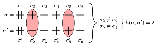
Figure 3: Hamming distance between two different many-body configurations of a 6-site 1D chain. The configurations are different at two sites, hence their Hamming distance is 2.

The absolute value in the denominator, $|r_{i}-r_{0}|^{\gamma}$, measures how far apart on the lattice is site $i$ (at position $r_{i}$) from a reference site $0$ (at position $r_{0}$) that is chosen arbitrarily. For a positive value of $\gamma$, this expression suppresses differences between sites that are distant from the reference, favoring short-range correlations. For translationally invariant systems, the choice of the reference site is irrelevant, while for systems without symmetry, an additional sum over all possible reference sites should be added in Equation 25. The second hyperparameter, $\theta$, is best understood by taking the Taylor expansion of Equation 25, that is

$$k(\bm{\sigma},\bm{\sigma}^{\prime})=1-\underbrace{\frac{\sum_{i}1-\delta_{\sigma_{i},\sigma_{i}^{\prime}}}{\theta}}_{\text{1-site correlation}}+\underbrace{\frac{\sum_{i,j}(1-\delta_{\sigma_{i},\sigma_{i}^{\prime}})(1-\delta_{\sigma_{j},\sigma_{j}^{\prime}})}{2\theta^{2}}}_{\text{2-site correlation}}+\ldots$$ (27)

where we omitted from the expansion the term $|r_{i}-r_{0}|^{\gamma}$ for clarity. Equation 27 shows how the kernel computes correlation features of increasing order (or rank) between the configurations. The first non-trivial term compares sites one by one, hence extracting 1-site correlation features. The second term compares sites in pairs, hence capturing 2-site correlation features, and so forth. This order-by-order comparison is graphically exemplified in Figure 4.

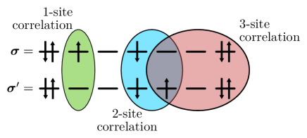
Figure 4: Correlation features identified by the kernel. Note that $n$-site correlation features with $n>1$ are not only compared between groups of $n$ neighboring sites, but with all possible combinations of $n$ sites.

With this understanding of the kernel, the denominator of Equation 27 unfolds the role of $\theta$ in suppressing higher-rank correlation features for values larger than 1. On the other hand, the opposite happens for $\theta<1$. The expansion in Equation 27 also reveals a key feature of the kernel function. Truncation of the sum to a fixed order allows the GPS to reproduce other known wavefunction ansätze. For instance, a first-order truncation corresponds to a Gutzwiller-type wavefunction [51], where only single-site occupancies are compared. Keeping only the second-order term, a generalized Jastrow representation is recovered [40], correlating all possible site pairs. Other, more general ansätze can also be expressed through the GPS by restricting site comparisons within a maximum range from the reference site. This generates, for instance, entangled plaquette states [52] and correlator product states [53]. All these traditional approaches explicitly parametrize the wavefunction in a particular feature space by constraining the rank or the range of the correlations modeled (note that this is analogous to the excitations classes of quantum chemical methods such as CCSD, where the singles would correspond to 1-site correlations, the doubles to 2-site correlations, and so forth). In strong contrast, the GPS implicitly extracts these features from the full kernel through the parameters associated to the reference configurations $\{\bm{\sigma}_{b}\}_{b=1}^{N_{b}}$. Crucially, while the number of multi-site features increases exponentially with the number of sites, the evaluation of Equation 25 only scales polynomially, highlighting the advantage of this kernel-based approach over explicit parametrizations. Furthermore, such a representation always ensures that the exact wavefunction can be obtained in the limit of the complete set of reference configurations (the complete set would correspond to a full CI).

Representational power of GPS.
Before discussing the optimization of the GPS in a variational framework, it is instructive to investigate the representational power of this ansatz by approximating an exact wavefunction in a supervised fashion. In particular, for a fixed choice of basis configurations $\{\bm{\sigma}_{b}\}_{b=1}^{N_{b}}$ and hyperparameters $\theta$ and $\gamma$, the GPS ansatz can be trained within a Bayesian inference framework with a set of training configurations and associated wavefunction amplitudes $\{\bm{\sigma}_{t},\psi(\bm{\sigma}_{t})\}_{t=1}^{N_{t}}$. In practice, the actual GP is the logarithm of Equation 24, that is

$$\varphi_{GPS}(\bm{\sigma})=\ln(\psi_{GPS}(\bm{\sigma}))=\sum_{b=1}^{N_{b}}w_{b}k(\bm{\sigma},\bm{\sigma}_{b}^{\prime})$$ (28)

and this model is trained on the log-amplitudes, $\varphi(\bm{\sigma}_{t})=\ln(\psi(\bm{\sigma}_{t}))$, rather than directly on the wavefunction amplitudes. The optimal parameters $w_{b}$ are then obtained as the mean of the posterior distribution for the weights according to Bayes theorem. This corresponds to a direct minimization of the squared error between the exact log-amplitudes and the predicted ones

$$\mathbf{w}^{*}=\operatorname*{argmin}_{\mathbf{w}}\sum_{t=1}^{N_{t}}\frac{|\varphi(\bm{\sigma}_{t})-\varphi_{GPS}(\bm{\sigma}_{t})|^{2}}{\sigma_{t}^{2}}$$ (29)

where $\sigma_{t}^{2}$ is a variance hyperparameter that regulates how tightly the GP reproduces the exact log-amplitudes at the training points (see [36] for a more detailed discussion). With such a scheme, it is possible to evaluate how accurately the GPS can represent the wavefunction of a known quantum state as a function of the number of basis configurations. For example, the plot in Figure 5 shows the mean squared error of the GPS with respect to the exact ground state of the 8-site Fermi-Hubbard model in the strong correlation regime ($U/t=8$).

Figure 5: Mean squared error between the GPS ansatz and the exact ground state of the Fermi-Hubbard model on an 8-site lattice. The hyperparameters $\gamma$, $\theta$ and $\sigma_{t}$ have been fixed a priori. Each point represents a random selection of $N_{b}$ basis configurations and the associated error. The color of the points represents the value of the log marginal likelihood for the weights, with red denoting larger values and blue smaller values. The dashed line and the black point show the accuracy reached by the RVM algorithm. The color-map is rescaled in the insets. Figure taken from [36] [36] (DOI: 10.1063/5.0024570).

As can be seen, the choice of basis configurations plays a crucial role for the accuracy of the GPS ansatz. In particular, for a basis set containing a few many-body configurations, the error can vary across several orders of magnitude, whereas for large basis sets the accuracy of the wavefunction is much more consistent. This can be understood in terms of the implicit parametrization of the wavefunction through the data $\{\bm{\sigma}_{b}\}_{b=1}^{N_{b}}$; a representative set of many-body configurations is needed for modeling the most important correlation features. It is thus clear from Figure 5 that the choice of the basis is paramount to obtain a compact and accurate representation of the wavefunction. A way to identify an optimal basis set $\{\bm{\sigma}_{b}\}_{b=1}^{N_{b}}$ is provided by relevance vector machine (RVM), a sparsification algorithm that selects the configurations based on the log marginal likelihood for the weights. Large values of the latter are associated to important configurations, whereas the opposite is true for small values. The RVM can thus be used to select the most representative $\bm{\sigma}_{b}$’s out of a set of candidate configurations, yielding an optimally compact basis set. An example of this can be seen in Figure 5, where the RVM algorithm produces a GPS that is significantly more accurate than the random selection, for a fixed number of basis configurations. Whereas the RVM algorithm is used to select the basis set, the optimization of $\theta$ and $\gamma$ can be done through a sampling of the hyperparameters space via a Bayesian scheme. In this optimization procedure, an initial assumed distribution is used to sample the hyperparameters, and gets refined after each iteration with the additional information obtained from the sampled points.

Bootstrapped Optimization.
After establishing that the GPS is able to compactly represent complicated wavefunctions, we shall turn to the case where the target quantum state is not known a priori. In this case, the parameters $w_{b}$ can be optimized by minimizing the energy expectation value according to the variational principle. In absence of data, an initial random set of basis configurations $\{\bm{\sigma}_{b}^{(0)}\}$ underpinning the GPS model is selected, and the associated weights $w_{b}$ are initialized to zero. Alternatively, a mean-field or another approximate wavefunction can be used to pre-train the weights of the GPS, providing a better starting point. Then, the values of the weights are optimized by minimizing the energy of the system. Similar to neural-network quantum states, the GPS ansatz models the wavefunction amplitudes of a quantum state, such that to evaluate the energy expectation value, the GPS needs to be projected on a particular basis or sampled according to a stochastic technique such as variational Monte Carlo. Next, the reference set of configurations $\{\bm{\sigma}_{b}^{(0)}\}$ is pruned through the RVM sparsification procedure, reducing the size of the basis while keeping the accuracy. New many-body configurations that are different from the initial ones then added to the basis, yielding a new reference set $\{\bm{\sigma}_{b}^{(1)}\}$. Here, there are various criteria that can be used to enlarge the basis set, for instance one could select configurations associated to a large uncertainty of the GPS (obtained through the Bayesian framework, see chapter 10), to a high local energy, or to a large variance contribution to the local energy. Regardless of the data augmentation criterion used, the weights of the new enlarged set are then optimized again variationally, and this process is repeated until convergence. A scheme depicting the optimization steps can be seen in Figure 6.

Figure 6: Bootstrap optimization steps of the GPS ansatz with the possible algorithmic choices on the right-hand side.

The optimization procedure just outlined was used to obtain the ground state of the half-filled Fermi-Hubbard model in one and two dimensions in the strong correlation regime with $U=8t$ [35]. For the one-dimensional chain with 32 sites, the GPS ansatz reached a relative energy error (with respect to DMRG) of $1.2\times 10^{-3}$ Hartree with 1369 reference many-body configurations. On a $6\times 6$ square lattice, the GPS systematically converges toward the exact ground state energy with increasing number $N_{b}$ of basis configurations. Both standard approaches based on the Gutzwiller wavefunction and Jastrow with pair correlations are easily surpassed in accuracy with less than 100 basis configurations, and the results obtained are on-par with the NQS ansatz (based on the RBM architecture) using a similar number of variational parameters. Instead, for the larger $8\times 8$ square lattice, the GPS initialized with a Jastrow wavefunction outperforms the RBM both in accuracy and convergence rate from the outset. In this case the GPS (with a number of parameters ranging from 1000 and 2000, depending on the RVM procedure) consistently shows a lower energy per site throughout the optimization procedure compared to the Gutzwiller (1 parameter), the Jastrow (34 parameters) and the RBM (2064 parameters, $\alpha=16$) ansätze.

Towards quantum chemical applications of GPS
The GPS ansatz has been initially used to obtain the ground state of the Fermi-Hubbard model, however, extensions to tackle the ab initio electronic Hamiltonian are in principle possible. For instance, following the approach of [27] used for NQS wavefunctions, spin orbital occupation numbers could be used to define the local Hilbert spaces of the many-body configurations. While this does not impose any particular restriction on the type of interactions captured by the RBM (thanks to the non-local nature of the inter-layer connections), extra attention is required for the GPS model. In particular, there are several ways to account for the dependence of the kernel on the distance between the sites, see the denominator of Equation 25. The spin orbitals could simply be mapped onto a one-dimensional lattice like a matrix product state wavefunction, however this would artificially bias the range of interactions captured by the kernel in an arbitrary way. On the other hand, if a basis of localized orbitals is used, the Euclidean distance between their centers in real space could be used directly in Equation 25. Another issue is the choice of reference site. Whereas all the sites in a regular lattice with periodic boundary conditions are equal, the same is not true for the single-particle basis used for molecules.

Despite these technical details, the GPS ansatz has shown to be a very promising alternative to other novel ML-based wavefunction approaches such as NQSs. Above all, the data-driven property intrinsic to non-parametric approaches is extremely appealing. Instead of constantly modifying the parametrization of the wavefunction (e.g. increasing the hidden-unit density of an RBM) and rerunning a calculation to reach a desired accuracy, the GPS ansatz can be systematically refined by the simple addition of new basis configurations and an extra iteration step, picking up increasingly complex many-body correlation features. Compared to traditional quantum chemical methods, the same discussion carried out for the NQS ansatz applies here as well. For instance, the limitations intrinsic to one-particle basis sets are present in this case, which is the price to pay for a method defined in the second quantization framework. On the other hand, the antisymmetry requirement is intrinsically satisfied by the many-body configurations basis. In order to encode the phase of the wavefunction, complex weights can be used as it was the case for RBMs. To avoid the use of complex algebra, alternative strategies to encode the phase need to be developed. At last, it can be envisioned that the GPS will probably find application as an active space solver in multireference settings, or for accurate benchmark calculations beyond what is currently feasible with full CI and similar approaches.

2.3 Modeling the wavefunction in real space

In the previous subsection we have seen how parametric and non-parametric machine learning methods have been used to represent the wavefunction in Fock space. A formalism based on second quantization has the great advantage that the Fermi-Dirac statistics is incorporated by construction in the many-particle basis, e.g. by Slater determinants for typical quantum chemical approaches. The same is not true for first-quantized methodologies. In fact, a major obstacle for modeling fermionic wavefunctions directly in real space is the proper integration of the antisymmetry property in the ansatz. In this subsection we shall see two examples of neural network architectures that have succeeded in this respect, with very promising results.

2.3.1 FermiNet

The indistinguishability of fermions manifests itself in a wavefunction that must be antisymmetric with respect to the exchange of two particles, as shown in Equation 6. Traditional quantum chemistry methods incorporate this property by introducing a basis of many-particle functions that satisfy this requirement, namely Slater determinants. These have the following general form

$$\Phi(\mathbf{r})=\mathcal{\hat{A}}\prod_{i=1}^{N}\phi_{i}(\mathbf{r}_{i})=\begin{vmatrix}\phi_{1}(\mathbf{r}_{1})&\ldots&\phi_{N}(\mathbf{r}_{1})\\ \vdots&&\vdots\\ \phi_{1}(\mathbf{r}_{N})&\ldots&\phi_{N}(\mathbf{r}_{N})\end{vmatrix}$$ (30)

where $\phi_{i}(\mathbf{r}_{j})$ are one-particle functions (spin orbitals) and $\mathcal{\hat{A}}$ is an antisymmetrizer that sums over all possible pairwise permutations of the particles, multiplied by either $+1$ or $-1$ depending on the parity of the permutation. This construct automatically satisfies Equation 6, and conveniently encodes the exchange of two particles, say $\mathbf{r}_{i}$ and $\mathbf{r}_{j}$, by swapping rows $i$ and $j$ in the determinant. It is this exactly property that stands at the heart of FermiNet.

The ansatz.
FermiNet is a wavefunction ansatz based on a deep neural network architecture [28]. The main idea underlying it comes from the realization that the basis functions $\phi_{i}(\mathbf{r}_{j})$ in Equation 30 do not necessarily have to be single-particle orbitals. The only requirement is that the wavefunction changes sign upon exchange of two rows in the determinant. With this observation, the orbitals $\phi_{i}(\mathbf{r}_{j})$ can actually be replaced by many-electron functions of the form

$$\phi_{i}(\mathbf{r}_{j};\mathbf{r}_{/j})=\phi_{i}(\mathbf{r}_{j};\mathbf{r}_{1},\ldots,\mathbf{r}_{j-1},\mathbf{r}_{j+1},\ldots,\mathbf{r}_{N})$$ (31)

with the property that swapping the positions $\mathbf{r}_{k}$ and $\mathbf{r}_{l}$ of any two particles with $k\neq l\neq j$, leaves the sign of $\phi_{i}(\mathbf{r}_{j};\mathbf{r}_{/j})$ unchanged. Slater determinants constructed with these permutation-equivariant functions, $\tilde{\Phi}(\mathbf{r})=\mathcal{\hat{A}}\prod_{i=1}^{N}\phi_{i}(\mathbf{r}_{i};/\mathbf{r}_{i})$, have a much larger expressive power than the ones constructed from single-particle orbitals. In fact, such a generalized Slater determinant (GSD) is in principle sufficient to represent any $N$-electron fermionic wavefunction [28, 54]. Nevertheless, the accuracy depends ultimately on the choice of the many-particle functions $\phi_{i}(\mathbf{r}_{j};\mathbf{r}_{/j})$, such that in practice using a small linear combination of GSDs is advantageous. The main innovation of the FermiNet ansatz is to express the wavefunction by a linear combination of these generalized Slater determinants

$$\Psi_{FermiNet}(\mathbf{r}) =\sum_{I=1}^{M}C_{I}\tilde{\Phi}_{I}(\mathbf{r})$$ (32)

$$=\sum_{I=1}^{M}C_{I}\left(\mathcal{\hat{A}}\prod_{i=1}^{N}\phi_{i}^{I}(\mathbf{r}_{i};/\mathbf{r}_{i})\right)$$

using many-particle “orbitals” $\{\phi_{i}^{I}(\mathbf{r}_{j};\mathbf{r}_{/j})\}$ represented by a deep neural network. Note that a different set of equivariant functions $\{\phi_{i}^{I}(\mathbf{r}_{j};\mathbf{r}_{/j})\}$ is used for each GSD $\tilde{\Phi}_{I}$ in the superposition, which are indexed by the superscript $I$. Importantly, although Equation 32 and Equation 4 look the same at first sight, the former contains determinants which are able to describe complicated many-body correlation effects through non-linear interactions between all electrons in each of the many-particle orbitals $\phi_{i}^{I}(\mathbf{r}_{j};\mathbf{r}_{/j})$. Hence, only a few determinants are sufficient to recover almost completely the electron correlation. The resulting architecture encoding the wavefunction is shown in Figure 7.

Figure 7: The neural network architecture underlying the FermiNet ansatz. Image adapted from [28] [28] (DOI: 10.1103/PhysRevResearch.2.033429).

To preserve the equivariance of the functions, FermiNet takes as input electron-nuclear and electron-electron relative coordinates and distances, and propagates through the network parallel streams of one-electron and two-electron feature vectors $\mathbf{h}_{i}^{l}$ and $\mathbf{h}_{ij}^{l}$, respectively. Similar equivariant architectures have been adopted in other machine learning approaches for computational chemistry, such as the SchNet neural network [55, 56] discussed in chapter 12. At each intermediate layer, these vectors are constructed by taking averages over same-spin features, $\mathbf{g}_{i}^{l\sigma}$ with $\sigma\in\{\uparrow,\downarrow\}$, which are concatenated to the distances and the output of the previous layer before passing through a non-linear activation function. It is this repeated process through the network that captures the correlation between the particles. In the last layer, the determinants $\tilde{\Phi}_{I}(\mathbf{r})$ are constructed, and their linear combination produces the final wavefunction value for a given set of input electronic and nuclear coordinates. Owing to the non-linearity and complexity of the ansatz, the optimization of the parameters relies on variational Monte Carlo, essentially following the strategy outlined at the beginning of the Methods section. However, in contrast to typical VMC wavefunction ansätze, FermiNet does not embed any prior physical information, e.g. the shape of the electron-electron cusp usually modeled by the Jastrow factor. This fact leads to a more difficult optimization procedure, such that pre-training is necessary to ensure convergence. For instance, the many-electron orbitals can be pre-trained by minimizing the least-square error to reference Hartree-Fock orbitals obtained in a finite basis set calculation.

Quantum chemical applications.
FermiNet was tested on a variety of atomic and molecular systems [28]. Ground state energies within chemical accuracy from the exact result [57] and at most a few m$E_{\text{h}}$ from CCSD(T) at the complete basis set (CBS) limit were obtained for first-row atoms, lithium through neon. Because FermiNet expresses the wavefunction directly in continuous space, there is no one-particle basis set and thus the concept of basis set limit ceases to exist in this framework. This is one of the major advantages with respect to a formalism based on second quantization. In comparison to a full CI wavefunction, the counterpart of the CBS extrapolation would be the limit of the network to an infinite number of layers. In small molecules containing two non-hydrogen atoms, FermiNet consistently recovers more than $99\%$ of the correlation energy, while in larger molecular systems — methylamine, ozone, ethanol and bicyclobutane — between $97\%$ and $98\%$. For all these systems, it outperforms CCSD(T) in finite basis sets of augmented quadruple and quintuple zeta quality, highlighting the superb accuracy that can be reached with this ansatz. The decline of the correlation energy recovered for larger systems could be hinting at a problem with the size-extensive property of FermiNet. However, all calculations were performed at a fixed network architecture, such that the variational degrees of freedom were the same regardless of the size of the systems considered. In contrast, traditional methods such as CCSD(T), implicitly increase their flexibility through the basis sets; for a fixed basis set quality, the number of basis functions depends on the size of the molecule, such that for a size-extensive approach, the fraction of correlation energy recovered should always be approximately the same. The true power of FermiNet unfolds when considering systems with significant strong correlation components. Here, the flexibility of the neural network architecture allows for an accurate description of prototypical systems such as the H_4 rectangle, the dissociation of N_2 and the H_10 hydrogen chain. In all these cases, single-reference techniques such as coupled cluster fail, and theoretical approaches considered state-of-the-art are instead auxiliary-field quantum Monte Carlo [58] and multireference configuration interaction. Once again, FermiNet delivers results which are on-par with the best methodologies available [28]. For instance, in the dissociation of N_2, the average error was about 5 milliHartree with respect to the experimental curve, comparable to the highly accurate $r_{12}$-MR-ACPF results. In the case of the hydrogen chain, stretching it from an internuclear distance of 1 atomic unit up to 3.5, resulted in errors with respect to MRCI+Q+F12 of less than 5 milliHartree, comparable to auxiliary-field quantum Monte Carlo at the complete basis set limit. The hydrogen chain was also used to investigate the effects of the network architecture on the accuracy of FermiNet. Here, it was found that the overall accuracy increases as more layers are added to the network, suggesting that a deep architecture is advantageous over a shallow, single-layer one. On the other hand, increasing the the width of the layers also provided generally improved results.

Computational complexity.
Compared to conventional quantum chemical approaches, the evaluation of the computational complexity of a neural-network-based ansatz is less straightforward. The total number of parameters in FermiNet is approximately given by $\mathcal{O}(N_{s}n_{h}+Ln_{h}^{2}+N_{s}^{2}M+N_{s}n_{h}M+M)$, where $N_{s}$ represents the size of the system (number of electrons or atoms), $n_{h}$ the number of hidden units, $L$ the number of layers and $M$ the number of determinants. There are three terms that scale with the size of the system, the largest one does so quadratically. The remaining terms are fixed for a given choice of network architecture. The evaluation of a single forward pass requires at most $\mathcal{O}(N_{s}^{3}(M+n_{h})+LN_{s}^{2}n_{h}^{2})$ operations, where the first term will dominate for larger system sizes at a fixed network architecture. Evaluation of the local energy needed in the VMC framework requires the calculation of the Laplacian, which scales with an extra factor of the system size. The optimization procedure requires a matrix inversion, with the largest component given by a term that scales as $\mathcal{O}(M^{3}N_{s}^{6})$. Overall, for a single optimization step, the scaling besides the matrix inversion is a quartic power with respect to the system size (local energy evaluation), which is to be compared to, for instance, the seventh power in CCSD(T), and exponential for full CI. While this analysis provides some theoretical ground on the computational complexity behind FermiNet, in practice it is easier to provide actual numbers for the performed calculations [28]. In particular, for all the results discussed above, the architecture included approximately $700000$ parameters, with resulting training times (i.e. wavefunction optimizations) between a few hours for the smaller systems, up to a month for bicyclobutane using 8 to 16 GPUs.

2.3.2 PauliNet

Another successful example of deep neural network ansatz defined in continuous space is PauliNet [29]. While the functional form underlying FermiNet is completely general, in the sense that it does not include any known physical feature of the wavefunction besides the antisymmetry, PauliNet follows a more traditional VMC approach, where deep neural networks are used to model certain components of the ansatz.

The ansatz.
PauliNet is a wavefunction ansatz of the Slater-Jastrow-backflow type, and is given by

$$\Psi_{PauliNet}(\mathbf{r}) =e^{\gamma(\mathbf{r})+J(\mathbf{r})}\sum_{I=1}^{M}C_{I}\tilde{\Phi}_{I}(\mathbf{r})$$ (33)

$$=e^{\gamma(\mathbf{r})+J(\mathbf{r})}\sum_{I=1}^{M}C_{I}\left(\mathcal{\hat{A}}\prod_{i=1}^{N}\phi^{I}_{i}(\mathbf{r}_{i})\xi^{I}_{i}(\mathbf{r})\right)$$

There are essentially four components that make up $\Psi_{PauliNet}(\mathbf{r})$. The first two appear in the exponential factor in front of the sum: $\gamma(\mathbf{r})$ is a function that directly models the electronic cusp of the wavefunction, while $J(\mathbf{r})$ is a Jastrow factor, which captures the short-range electron correlation effects. The third component is the fixed linear superposition of (a few) Slater determinants, which enforces the antisymmetry requirement of fermions. The one-particle orbitals $\phi_{i}(\mathbf{r}_{j})$ are standard Gaussian orbitals, that are obtained by a Hartree-Fock or small complete active space SCF calculation. The orbitals are multiplied by the fourth component, which are the backflow functions $\xi_{i}^{I}(\mathbf{r})$ (note the dependence on all electronic coordinates). As explained in the introduction to the VMC approach in the beginning of the Methods section, such a transformation is crucial to improve the nodal surface fixed by the Slater determinants. However, contrary to Equation 12, the backflow transformation in PauliNet does not substitute the individual electronic coordinates in $\phi_{i}(\mathbf{r}_{j})$ by the corresponding backflow-transformed ones, but rather, it directly multiplies the orbitals by many-electrons equivariant functions $\xi_{i}^{I}(\mathbf{r})$. This choice leads to a simpler and more efficient optimization of the backflow parameters. The main innovation in the ansatz of Equation 33 is the fact that the Jastrow factor $J(\mathbf{r})$ and the backflow transformation functions $\xi_{i}^{I}(\mathbf{r})$ are represented by deep neural networks, providing a very flexible functional form for modeling both the electron correlation and the nodal surface of the wavefunction. For Equation 33 to remain a valid wavefunction, the various components need to satisfy different constraints. To maintain the cusp conditions enforced by $e^{\gamma(\mathbf{r})}$, the neural networks parametrizing the Jastrow factor and the backflow transformation are constructed cusp-less, that is, satisfying

$$\nabla_{\mu_{i}}J(\mathbf{r})\Big{|}_{\mu_{i}=\{\mathbf{r}_{k},\mathbf{R}_{K}\}} =0$$ (34)

$$\nabla_{\mu_{i}}\xi_{i}^{I}(\mathbf{r})\Big{|}_{\mu_{i}=\{\mathbf{r}_{k},\mathbf{R}_{K}\}} =0$$ (35)

Furthermore, to preserve the antisymmetric nature of $\Psi_{PauliNet}(\mathbf{r})$ imposed by the Slater determinants, $\gamma(\mathbf{r})$ and $J(\mathbf{r})$ are invariant with respect to the exchange of pair of particles, that is

$$\gamma(\mathcal{P}_{ij}\mathbf{r}) =\gamma(\mathbf{r})$$ (36)

$$J(\mathcal{P}_{ij}\mathbf{r}) =J(\mathbf{r})$$ (37)

where $\mathcal{P}_{ij}$ is the operator exchanging particles $i$ and $j$. On the other hand, the backflow transformation functions $\xi_{i}^{I}(\mathbf{r})$ are equivariant, i.e.

$$\mathcal{P}_{ij}\xi_{i}^{I}(\mathbf{r})=\xi_{j}^{I}(\mathcal{P}_{ij}\mathbf{r})$$ (38)

The invariance and equivariance properties encoded in Equation 37 and Equation 38, respectively, and the the many-particle dependence of the electronic interactions are analogous to the requirements for learning potential energy surfaces with neural networks. Taking advantage of this similarity, another level of complexity is introduced in the PauliNet architecture by transforming the electronic coordinates through a modified version of SchNet [56], before they are fed to the Jastrow factor and backflow transformation. In practice, SchNet projects each electronic coordinate onto a features space of dimension $D_{e}\gg 3$, that encodes many-body correlations between the particles. These high-dimensional representations, $\mathbf{x}_{i}(\mathbf{r})$, are then used as input to the Jastrow and backflow functions

$$J(\mathbf{r}) =\eta\bigg{(}\sum_{i=1}^{N}\mathbf{x}_{i}(\mathbf{r})\bigg{)}$$ (39)

$$\bm{\xi}_{i}^{I}(\mathbf{r}) =\bm{\kappa}\bigg{(}\sum_{i=1}^{N}\mathbf{x}_{i}(\mathbf{r})\bigg{)}$$ (40)

The functions $\eta(\cdot)$ and $\bm{\kappa}(\cdot)$ are modeled by deep neural networks, with trainable parameters. The electronic cusps, the Slater determinants with backflow transformed coordinates and the Jastrow factor are then combined together to yield the value of the wavefunction amplitude. The overall PauliNet architecture is summarized in Figure 8, which shows a simplified version of the ansatz (see [29] for a more comprehensive figure).

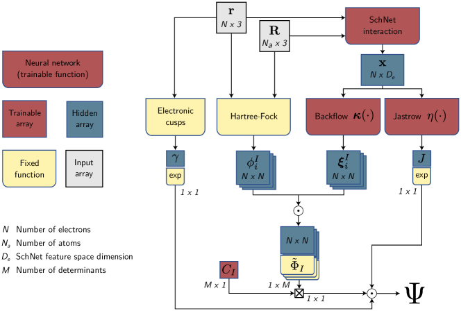
Figure 8: Simplified scheme depicting the structure of the PauliNet ansatz.

The sophisticated architecture of PauliNet reflects the many physical components directly included in the ansatz. Importantly, while these constrain its functional form, they do so without restricting its representational power for modeling the wavefunction associated to a quantum state. The various (fixed) components actually provide a blueprint, upon which the deep neural networks describing the electronic embeddings, the Jastrow factor and the backflow transformation provide sufficient flexibility. The optimization of the variational parameters underpinning PauliNet is carried out in the framework of VMC. While the method to sample the configurations and the technique to minimize the energy slightly differ from the ones introduced above, the overall strategy is the same.

Quantum chemical applications.
PauliNet is able to recover between $97\%$ and $99.9\%$ of the correlation energy of several atomic and diatomic systems, such as H_2, LiH, Be and B [29]. This is achieved by training the neural networks for at most a few hours on a single GPU. This fact highlights an important difference with respect to the more flexible FermiNet architecture. That is, the incorporation of the physical components of a wavefunction in PauliNet (mean-field orbitals, electronic cusp, and so forth) allows for a much faster optimization of the parameters. The dependence of the energy with respect to the number of determinants in Equation 33 was assessed on four diatomic molecules, Li_2, Be_2, B_2 and C_2 [29]. It was found that PauliNet systematically recovers a larger fraction of the correlation energy by increasing number of SDs, reaching the accuracy of state-of-the-art diffusion Monte Carlo calculations with a much shorter linear superposition compared to other VMC ansätze. The use of a finite basis set for the mean-field orbitals appears to introduce a basis set dependence in the calculation, which is a typical source of error in traditional quantum chemical methods. Whereas CBS extrapolations are required for the latter approaches, PauliNet is not sensitive to the choice of basis set for the orbitals $\phi_{i}^{I}(\mathbf{r}_{j})$ thanks to the deep backflow transformation, which is able to compensate for the missing flexibility in the basis [59]. Convergence to the fixed-node limit, i.e. capturing all electron correlation without modifying the position of the wavefunction nodes, can also be reached by PauliNet. In particular, it was shown that for both LiH and H_4, chemical accuracy can be quantitatively reached by increasing the number of layers and their width in the deep Jastrow factor [59]. Similarly to FermiNet, PauliNet is able to capture strong electron correlation as well. For the challenging H_10 hydrogen chain, $98.4\%$ of the correlation energy was recovered for both the equilibrium and the stretched geometries, using a total of 16 determinants. The ansatz performed extremely well also in combination with a single SD, with a slightly less amount of $97.5\%$ of correlation energy captured. While the calculations on small systems have shown that PauliNet can reach chemical accuracy and surpass traditional quantum chemical methods, it also scales to larger molecules. For instance, an investigation on the automerization of cyclobutadiene, a molecule with 28 electrons, provided results on-par with the best theoretical estimates for the barrier, albeit with a smaller uncertainty interval. Formally, the most expensive step in PauliNet is the evaluation of the kinetic energy at the sample points, which scales as $\mathcal{O}(N^{4})$, with $N$ being a measure of the system size. This is the standard computational complexity in variational Monte Carlo, and the presence of the deep neural networks does not change it.

2.4 Supervised machine learning of the wavefunction

In the last two subsections we have seen examples of how machine learning models can be used to represent the wavefunction ansatz directly, either in Fock space or real space, and how these can be efficiently optimized through variational Monte Carlo. In this subsection we shall instead discuss a very different approach to the quantum many-body problem, whereby the wavefunction is learned in a supervised fashion.

2.4.1 SchNOrb

In electronic structure theory, the simplest description of a molecular system is provided by a single SD wavefunction. This is constructed from an antisymmetrized product of single-particle functions as discussed in the previous sections (cfr. Equation 30), which are typically expanded in a linear combination of $N_{AO}$ local atomic orbitals (AOs) as

$$\phi_{i}(\mathbf{r})=\sum_{\mu=1}^{N_{AO}}c_{\mu i}\chi_{\mu}(\mathbf{r})$$ (41)

where $\mathbf{r}$ now denotes the Cartesian coordinates of a single electron. Knowledge of the coefficients vectors $\{\mathbf{c}_{i}\}$ and associated orbital energies $\{\epsilon_{i}\}$ for a given basis set $\{\chi_{\mu}(\mathbf{r})\}_{\mu=1}^{N_{AO}}$ is sufficient to represent the wavefunction and the total energy, and therefore to give access to molecular properties of the modeled system as well. Hence, it might be tempting to train a machine learning model to reproduce these coefficients and energies for a prescribed atomic orbital basis set. However, in practice, the training process is particularly difficult because these are not smooth and well-behaved function of the nuclear coordinates, displaying degenerate energies, changes of the orbital ordering and an arbitrary dependence on the phase factor. Instead, learning directly the representation of the Hamiltonian operator in the atomic orbital basis, and the associated overlap matrix, leads to a much better behaved problem that essentially contains the same information. In fact, given the Hamiltonian matrix $\mathbf{H}$ and the overlap matrix $\mathbf{S}$ between the basis functions $\chi_{\mu}(\mathbf{r})$, the molecular orbital (MO) coefficients $\mathbf{c}_{i}$ and associated energies $\epsilon_{i}$ can be obtained by a simple diagonalization of the following generalized eigenvalue problem

$$\mathbf{H}\mathbf{c}_{i}=\epsilon_{i}\mathbf{S}\mathbf{c}_{i}$$ (42)

with the elements of $\mathbf{H}$ and $\mathbf{S}$ reading

$$\mathbf{H}_{\mu\nu} =\braket{\chi_{\mu}}{\hat{H}}{\chi_{\nu}}$$ (43)

$$\mathbf{S}_{\mu\nu} =\braket{\chi_{\mu}}{\chi_{\nu}}$$ (44)

In Equation 42 and Equation 43, $\mathbf{H}$ is either the Fock matrix from Hartree-Fock theory or the Kohn-Sham matrix from density functional theory. Note that the idea to learn the Hamiltonian and overlap matrices in a given basis is essentially the same as the approach taken in semi-empirical methods, whereby Equations 43 and 44 are parametrized against experimental data or higher-level ab initio calculations. The difference with SchNOrb lies in how this parametrization is done. As we will see, using a deep neural network leads to very accurate results.

The SchNOrb neural network.
SchNOrb is a deep learning framework in which the main idea is to learn the representation of the Hamiltonian and overlap matrices from a large set of reference calculations [33, 34]. This is achieved by training a deep convolutional neural network based on the SchNet architecture [55, 56]. The input consists of the atomic coordinates $(\mathbf{R}_{1},\ldots,\mathbf{R}_{N_{a}})$ and corresponding nuclear charges $(Z_{1},\ldots,Z_{N_{a}})$. Atomic representations are then constructed in a first stage following the classical SchNet architecture, yielding a set of high-dimensional feature vectors $\mathbf{x}_{i}^{(0)}$. The latter are passed on to the next stage, where a second deep convolutional neural network, SchNOrb, generates pair-wise atomic features

$$\bm{\Omega}_{ij}^{(l)}=\prod_{\lambda=0}^{l}\bm{\omega}_{ij}^{(\lambda)}$$ (45)

as products of $l$ symmetry-adapted polynomials of increasing order. This ensures that the rotational symmetry of the local orbitals up to angular momentum $l$ can be properly accounted for. In each layer $\lambda$ of SchNOrb, the polynomials $\bm{\omega}_{ij}^{(\lambda)}$ depend on the pairwise interaction between the atomic environments $\mathbf{x}_{i}^{(\lambda)}$ and $\mathbf{x}_{j}^{(\lambda)}$, and the interatomic distance between atoms $i$ and $j$. In this context, the polynomial coefficients $\mathbf{p}_{ij}^{(\lambda)}$ making up the $\bm{\omega}_{ij}^{(\lambda)}$’s can be thought of as the SchNOrb counterparts of the linear coefficients of the orbital expansions in traditional quantum chemical methods. The pairwise features $\bm{\Omega}_{ij}^{(l)}$ constructed in this way are then used to build the Hamiltonian $\mathbf{H}$ and overlap $\mathbf{S}$ matrix representations. Through the sequential passes in the layers of SchNOrb, the atomic environments $\mathbf{x}_{i}^{(\lambda)}$ are further refined and the output features vectors $\mathbf{x}_{i}^{(2L+1)}$ are used for the prediction of the total energy of the system $E_{tot}$. A schematic representation of the SchNOrb architecture is shown in Figure 9.

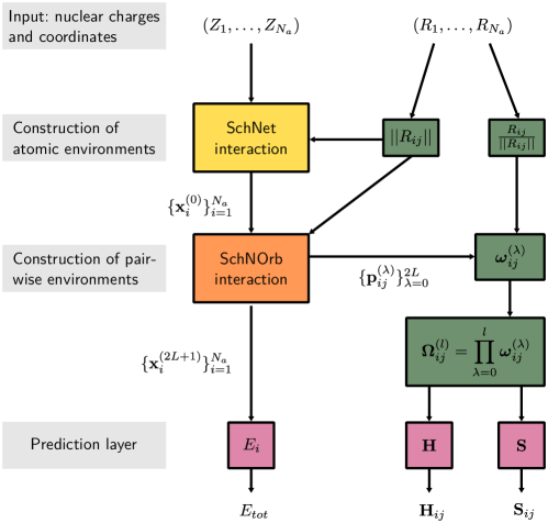
Figure 9: Simplified scheme depicting the SchNOrb deep neural network architecture. Green blocks are fixed functions, yellow and orange blocks are deep convolutional neural networks, and plum blocks are neural networks producing the final output.

Training and prediction.
The SchNOrb approach is a supervised learning algorithm. Reference data, that is, the Hamiltonian and overlap matrices computed at a given level of theory (basis set, method, functional), are generated by sampling the conformational space of the molecule and by performing actual quantum chemical calculations. The neural network is then trained with a combined regression loss given by

$$l(\tilde{\mathbf{H}},\tilde{\mathbf{S}},\tilde{E},\mathbf{H},\mathbf{S},E,\mathbf{F})=||\mathbf{H}-\tilde{\mathbf{H}}||_{F}^{2}+||\mathbf{S}-\tilde{\mathbf{S}}||_{F}^{2}+\rho||E-\tilde{E}||^{2}+\frac{1-\rho}{N_{a}}\sum_{i=1}^{N_{a}}\bigg{|}\bigg{|}\mathbf{F}_{i}-\bigg{(}-\frac{\partial\tilde{E}}{\partial\mathbf{r}_{i}}\bigg{)}\bigg{|}\bigg{|}^{2}$$ (46)

where the quantities with a tilde are the predicted values and $\rho$ determines the trade-off between energy and forces. The optimization is performed with standard procedures for training deep neural networks, such as stochastic gradient descent. For each molecule, several thousands geometries are necessary to properly sample the conformational space and learn the correct rotational symmetries. For instance, in the original work presenting SchNOrb [33], 25000 conformations were used for ethanol, malondialdehyde, and uracil. Once trained, the performance of the neural network can be evaluated by computing the mean absolute error between the prediction and reference calculations on a test set containing new conformations. An example of the accuracy that can be reached with SchNOrb is summarized in Table 2, for Hamiltonian and overlap matrices generated with either Hartree-Fock or DFT in combination with the PBE exchange and correlation functional and an atomic basis set including functions up to $d$ angular momentum.

Table 2: Mean absolute error of the SchNOrb prediction with respect to reference calculations of the Hamiltonian and overlap matrices, MO energies, occupied MO coefficients and total energies. The test set contained between 1500 and 4500 new conformations. Data taken from [33].

Molecule	Method	$\mathbf{H}$ [meV]	$\mathbf{S}$	$\epsilon$ [meV]	$\phi_{i}$	$E$ [meV]
Water	PBE	4.5	7.91e-05	7.6	1.00	1.435
Ethanol	HF	7.9	7.50e-05	10.6	1.00	0.378
Ethanol	PBE	5.1	6.78e-05	9.1	1.00	0.361
Malondialdehyde	PBE	5.2	6.73e-05	10.9	0.99	0.353
Uracil	PBE	6.2	8.24e-05	47.9	0.90	0.848

In all cases the accuracy is very good, with errors in the Hamiltonian matrix below 10 meV and in most cases below 1 meV for the total energy. Interestingly, the error observed for the orbital energies (a derived property that is not directly learned) is clearly distinct for occupied ($<20$ meV) and virtual orbitals ($\approx 100$ meV), probably due to the fact that the latter are not strictly defined in the HF or Kohn-Sham scheme. Molecular properties are also accurate, with both dipole and quadrupole moments reproduced with errors in the order of $0.055$ D and B, respectively. Note that the accuracy of SchNOrb is bounded by the level of theory with which the training data was generated. It would be desirable to have these in combination with an accurate quantum chemical methods and, in particular, large basis sets. However, larger bases imply an increased complexity and dimension of the Hamiltonian and overlap matrices. It was observed in this case, that while the prediction of the latter remained accurate, the derived properties suffered from an increased error. For instance, when the network was trained for ethanol in combination with a triple zeta basis, a mean absolute error in the MO energies of 0.4775 eV was found, highlighting the difficulty to learn the more complex representation [33]. This error can be traced back to the diagonalization of the Hamiltonian matrix, which in the larger basis accumulates the prediction error. A solution to this issue is the projection of the calculations onto a optimized minimal basis [34], which also has the advantage of shorter training times due to the reduced dimensionality of the data.

SchNOrb applications
All the ML wavefunction approaches seen in the previous subsections constitute novel ways to represent the complex functional form underlying a quantum state. While these are inspired by machine learning models, their practical application remains within a more traditional setting such as that of variational Monte Carlo. On the other hand, SchNOrb is an approach that follows the typical ML paradigm more closley, thereby learning the relation between molecular geometries and their quantum mechanical wavefunction representation from large amount of data. Because SchNOrb is bound to predict the wavefunction at an accuracy at most comparable to the method used to generate the training data, the type of applications targeted by this approach are different from the previous ones. Even more so, considering that creation of the training set and the network optimization requires a considerable amount of time. For instance, for all molecules considered in the original work [33], the training time was about 80 hours, and the creation of the training set took from 65 hours for ethanol, up to 626 hours for uracil. On the other hand, once the network is trained, the prediction is obtained in tens of milliseconds, compared to seconds or minutes for the traditional quantum chemical counterparts. In this perspective, it is clear that SchNOrb is an ideal candidate to carry out molecular dynamics simulations, at an accuracy well beyond that of classical force fields, but at a comparable computational cost after training. Other possible applications for SchNOrb could be to accelerate the convergence of traditional SCF calculations, use of SchNOrb orbitals for post-HF methods, or in inverse design, where a desired property could be optimized as a function of the nuclear positions [33].

3 Case Studies

In these cases studies we are going to use machine-learning-based methods to solve the Schrödinger equation. In the first case study, we will model the ground state wavefunction of a quantum-mechanical particle in a one-dimensional box using Gaussian process regression. This approach is similar in spirit to the Gaussian process state ansatz presented in the Methods section, however, we will model the wavefunction directly in real space rather than in Fock space. In the second case study, we are going to compute the ground state energy of the lithium hydride molecule using PauliNet, and analyze its dependence on the basis set used to generate the orbitals.

3.1 Particle in a Box

Let us start with the theoretical background for this problem. The Hamiltonian (in atomic units) to describe a quantum-mechanical particle confined in a one-dimensional box of length $L$ is given by

$$\hat{H}=-\frac{1}{2}\frac{\mathrm{d}^{2}}{\mathrm{d}x^{2}}+V(x)$$ (47)

where the potential function $V(x)$ is

$$V(x)=\begin{cases}0,&0<x<L\\ \infty,&\textrm{otherwise}\end{cases}$$ (48)

The exact ground state wavefunction for this Hamiltonian is known, and its analytical form reads

$$\Psi(x)=\begin{cases}\sqrt{\frac{2}{L}}\sin\left(\frac{\pi}{L}x\right),&0<x<L\\ 0,&\textrm{otherwise}\end{cases}$$ (49)

with the associated ground state energy

$$E=\braket{\Psi}{\hat{H}}{\Psi}=\int\Psi^{*}(x)\hat{H}\Psi(x)\mathrm{d}x=\frac{\pi^{2}}{2L^{2}}$$ (50)

The knowledge of the exact wavefunction will let us draw $N_{tr}$ random samples $\{x^{(i)},\Psi(x^{(i)})\}_{i=1}^{N_{tr}}$ and create a training set from which the underlying functional form of $\Psi(x)$ can be inferred from the data.

3.1.1 Bayesian learning of the wavefunction with a Gaussian process

In this case study, we define a wavefunction ansatz as the mean of a Gaussian process (GP)

$$\tilde{\Psi}(x)=\Phi_{GP}(x)=\begin{cases}\sum_{i=1}^{N_{s}}w_{i}k(x^{(i)},x),&0<x<L\\ 0,&\textrm{otherwise}\end{cases}$$ (51)

where we explicitly set to zero the wavefunction where the potential is infinite. We will use the squared exponential kernel

$$k(x,x^{\prime})=\exp\left(-\frac{|x-x^{\prime}|^{2}}{2l^{2}}\right)$$ (52)

as this provides simple analytical forms for the derivatives that we need for solving the electronic structure problem. The hyperparameter $l$ is called the length-scale, and controls the locality of the correlation between two points $x$ and $x^{\prime}$. For a large value of $l$, the kernel only correlates points very close to each other, and the opposite is true for a small value of $l$. While the value of this hyperparameter can in principle be optimized, we will not be concerned with that in this case study, instead we will use a fixed value. In the framework of Gaussian process regression, the vector of optimal weights can be obtained in closed form with the following expression

$$\mathbf{w}=(\mathbf{K}+\lambda\bm{1})^{-1}\bm{\Psi}$$ (53)

where $\mathbf{K}$ is the covariance matrix obtained by evaluating the kernel function between all training points, $\mathbf{K}_{ij}=k(x^{(i)},x^{(j)})$, $\bm{\Psi}$ is a vector with the amplitudes of the exact wavefunction evaluated at all training points, $\bm{\Psi}_{i}=\Psi(x^{(i)})$, and $\lambda$ is a small regularization hyperparameter that controls the variance of the model at the training points. For a value of $\lambda=0$, the Gaussian process will pass exactly through the data used to train it, while for larger values it does not necessarily has to. The wavefunction has to vanish at the edges of the box, that is $\tilde{\Psi}(0)=\tilde{\Psi}(L)=0$. Because the GP is an exact interpolator for $\lambda=0$, one way to enforce these boundary conditions (bc) is to (always) include in the training set these two points at the edges, $(x^{(1)}=0,\Psi(0)=0)$ and $(x^{(2)}=L,\Psi(L)=0)$. This will ensure that $\Phi_{GP}(x)$ will take on those values at the boundaries. We can now generate a few random training samples within the box and use these together with the bc points to fit the ground state wavefunction. To evaluate the accuracy of our model, we can compute the mean squared error between the exact wavefunction and the ansatz at the test points $\{\tilde{x}^{(i)}\}_{i=1}^{N_{pr}}$ (regularly spaced coordinates within the box)

$$\text{MSE}=\frac{1}{N_{pr}}\sum_{y=1}^{N_{pr}}\big{|}\tilde{\Psi}(\tilde{x}^{(i)})-\Psi(\tilde{x}^{(i)})\big{|}^{2}$$ (54)

As an exercise, plot the convergence of the error as a function of the number of training points $N_{tr}$, using different strategies to generate them: randomly draw them from a uniform distribution or place them equidistantly within the box. For this case study, you can use a box of length $L=5$, set the hyperparameter of the Gaussian kernel to $l=2$ and the regularization parameter $\lambda=0$. To carry out these exercises, we provide a self-contained implementation in Python based on the NumPy, SciPy and matplotlib libraries, presented as a jupyter notebook that can be downloaded from github.com/stefabat/MLWavefunction. However, as an advanced exercise, you can try to write the program from scratch yourself using your favorite programming language (hint: for Python use the NumPy function linalg.solve to invert the covariance matrix). You should obtain results similar to those shown in Figure 10.

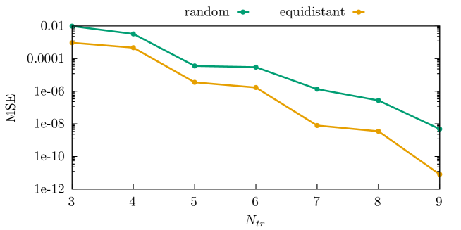
Figure 10: Convergence of the mean squared error in the wavefunction as a function of the training set size. The curve labeled “random” stands for the randomly generated training set, while the curve labeled “equidistant” stands for the training set generated on an equidistant grid of points.

One of the advantages of Gaussian processes is that they are defined with a Bayesian inference framework. This allows to construct confidence intervals about the model, that can tell us the uncertainty of the fitted function. In particular, we can calculate the confidence for a prediction of the wavefunction $\tilde{\Psi}(x)$ at a point $x$, based on the variance of the GP model using the following formula

$$\sigma^{2}(x)=k(x,x)-\mathbf{k}(x)^{T}(\mathbf{K}+\lambda\bm{1})^{-1}\mathbf{k}(x)$$ (55)

where $\mathbf{k}(x)$ is the vector function with elements $\mathbf{k}_{i}(x)=k(x^{(i)},x)$, with $x^{(i)}$ being the points of the training set. We can now use Equation 55 to plot the 95% confidence interval for each test point $\tilde{x}^{(i)}$, which approximately corresponds to twice the variance, that is, $\tilde{\Psi}(\tilde{x}^{(i)})\pm 2\sigma$. This is shown in Figure 11 for a randomly generated training set.

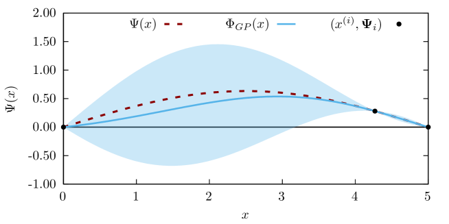
Figure 11: Gaussian process wavefunction trained on three points (black circles): a single randomly generated one within the box and two at the edges to ensure the proper boundary conditions. The shaded blue area is the 95% confidence interval of the Gaussian process. The length of the box is $L=5$, the GP hyperparameters are $l=2$ and $\lambda=0$.

As we can see from the plot, the uncertainty is zero at the training points because the GP passes right through them. On the other hand, maximum variance is attained at regions that are farthest away from the underlying data parametrizing the GP wavefunction.

3.1.2 Variational optimization of the Gaussian process wavefunction

In the second part of the first case study, we will optimize the Gaussian process wavefunction variationally, obtaining the optimal weights without the need to know the wavefunction a priori. To do so, it is first convenient to slightly change our ansatz of Equation 51, by explicitly incorporating the boundary conditions. This can be done by multiplying the GP with a function that satisfies the constraints, that is

$$f(x)=x(L-x)$$ (56)

yielding a new ansatz

$$\tilde{\Psi}(x)=\begin{cases}\Phi_{GP}(x)f(x),&0\leq x\leq L\\ 0,&\textrm{otherwise}\end{cases}$$ (57)

Note the explicit definition of $\Phi_{GP}(x)f(x)$ at the boundaries $x=0$ and $x=L$ included (in contrast to Equation 51). It is easy to test that $\tilde{\Psi}(x)=\Phi_{GP}x(L-x)$ at these points is exactly zero. The variational optimization of Equation 57 requires first an expression for the energy expectation value, i.e.

$$\tilde{E}=\frac{\Braket{\tilde{\Psi}}{\hat{H}}{\tilde{\Psi}}}{\Braket{\tilde{\Psi}}{\tilde{\Psi}}}=\frac{\Braket{\tilde{\Psi}}{-\frac{1}{2}\frac{\mathrm{d^{2}}}{\mathrm{d}x^{2}}+V(x)}{\tilde{\Psi}}}{\Braket{\tilde{\Psi}}{\tilde{\Psi}}}$$ (58)

Substitution of $\tilde{\Psi}(x)$ with Equation 57 results in the following double sum for the Hamiltonian expectation value in the numerator

$$\sum_{i=1}^{N_{s}}\sum_{j=1}^{N_{s}}w_{i}^{*}w_{j}\Braket{k(x^{(i)},x)f(x)}{\hat{H}}{k(x^{(j)},x)f(x)}=\sum_{i=1}^{N_{s}}\sum_{j=1}^{N_{s}}w_{i}^{*}w_{j}H_{ij}=\mathbf{w}^{T}\mathbf{H}\mathbf{w}$$ (59)

and similarly for the overlap in the denominator

$$\sum_{i=1}^{N_{s}}\sum_{j=1}^{N_{s}}w_{i}^{*}w_{j}\Braket{k(x^{(i)},x)f(x)}{k(x^{(j)},x)f(x)}=\sum_{i=1}^{N_{s}}\sum_{j=1}^{N_{s}}w_{i}^{*}w_{j}S_{ij}=\mathbf{w}^{T}\mathbf{S}\mathbf{w}$$ (60)

The evaluation of Equation 59 requires the second-order derivative of the $k(x^{(i)},x)f(x)$ with respect to $x$. Fortunately, the simple form of the squared exponential kernel we have selected admits an analytical expression, which is left as an exercise to derive. Furthermore, because the wavefunction ansatz is zero everywhere but within the box, we can restrict the domain of integration for the matrix elements to go from $0$ to $L$, where $V(x)=0$. In principle, the matrix elements can be obtained in closed form, however, for simplicity we will use numerical quadrature to perform the integration (hint: if you are writing the program from scratch, you can use the SciPy function integrate.quad). The last step required for the variational optimization of $\tilde{\Psi}(x)$ is to minimize the energy with respect to the weights $w_{i}$ of the GP. These act as the variational degrees of freedom of our ansatz. While the minimization of $\tilde{E}$ can be performed with common methods used in machine learning, such as (stochastic) gradient descent, for our simple example, it is more convenient to equate the derivative of the energy with respect to the weights, and explicitly solve the resulting generalized eigenvalue problem

$$\frac{\mathrm{d}\tilde{E}}{\mathrm{d}w_{i}}=0\;\text{for}\;i=1,\ldots,N_{tr}\iff\mathbf{H}\mathbf{w}=\tilde{E}\mathbf{S}\mathbf{w}$$ (61)

This is completely analogous to the way in which configuration interaction wavefunctions are optimized in quantum chemistry. Note that, as a byproduct, the diagonalization of $\mathbf{H}$ will also return the weights associated to the excited states of the particle. As an exercise, study the energy convergence of the GP wavefunction for increasing number of training points $N_{tr}$. As before, you can generate the points randomly or equidistantly within the box. Note that a training point in this context can be understood as the center of a new basis function used to represent $\tilde{\Psi}(x)$. You should get results similar to the ones shown in Figure 12.

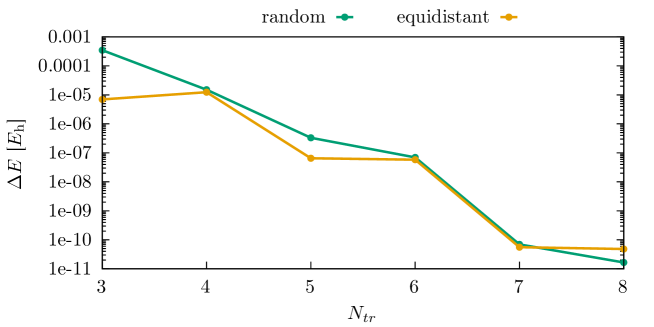
Figure 12: Ground state energy difference between the variationally optimized GP wavefunction and the exact solution for different training set sizes. The curve labeled “random” stands for the randomly generated training set, while the curve labeled “equidistant” stands for the training set generated on an equidistant grid of points.

As we can see, for such a simple system, there is not much difference in the energy convergence between the randomly generated training set and the equidistant one. In line with the GPS ansatz discussed in the Methods section, for a small training set, e.g. with $N_{tr}=3$, the training point within the box is very important for the accuracy. The randomly generated one yields a GP wavefunction with a significantly worse energy than with the training point placed at the center of the box.

3.2 Ground state energies from PauliNet

In this second case study we will compute the ground state energy of lithium hydride using PauliNet [29], investigate its dependence on the basis set used to generate the initial orbitals and compare it to highly-correlated CCSD(T) calculations. First, install the DeepQMC package following the installation guide at deepqmc.github.io. Note that the full package with all dependencies is more than 1GB of data. The installation of DeepQMC will also pull the quantum chemical library PySCF, which we will use to perform the coupled cluster calculations.

We provide a jupyter notebook written in python that walks you through this second case study, that can be downloaded from github.com/stefabat/MLWavefunction. However, you can also try to carry out the steps described below by yourself as an exercise.

3.2.1 PauliNet training

We are going to use the default PauliNet architecture and change the basis set to the correlation-consistent family [60], starting from cc-pvdz to cc-pv5z. The first step is to define a Molecule object (for example named LiH) with the geometry of LiH at an internuclear distance of $3.0141132$ Bohr, and a total zero charge and spin. Then, the PauliNet neural network can be initialized for a given basis set, say cc-pvdz, from a Hartree-Fock calculation using the function from_hf(LiH, basis=’cc-pvdz’), meaning that the ansatz contains a single Slater determinant (cfr. Equation 33) and uses the HF orbitals. After initialization, the network can be trained using the function train(net), where net is the neural network object returned from the initialization procedure. This is the most expensive part of the calculation, however, the training parameters can be slightly modified to decrease the computation time, and still obtain reasonably optimized network weights (with an uncertainty of around 1 m$E_{\text{h}}$). We suggest you to use n_steps = 500, batch_size = 500 and epoch_size = 20. The last step to obtain the ground state energy of LiH is to call the function evaluate(net). Similarly to train(net), evaluate(net) accepts optional parameters defining the number of Monte Carlo sweeps and the length of the Markov chain sampled at each step. For these two, we suggest the following values, n_steps = 400 and sample_size = 800. Save the obtained energy and the estimated error, and repeat the same process for the other basis sets. The choice of training parameters was such that the optimization does not take too long time. If you want to investigate the effects of the training procedure on the final energy and uncertainty, as an advanced exercise you can modify the values of n_steps and batch_size in the train(net) function (hint: modify one value at a time to understand their role).

3.2.2 CCSD(T) calculations

In this part we are going to perform CCSD(T) calculations in combination with the four basis sets used above. You can use PySCF for performing these calculations, and they should take significantly less time than the PauliNet ones. PySCF has a pretty extensive user guide available online at https://pyscf.org/, with many examples. We suggest you to have a look at it if you get stuck at any point. The first step is again to define the lithium hydride molecule, this time in a data-structure that PySCF understands. This can be done with the function gto.M(…), which accepts a number of arguments similar to the construction of the Molecule object for the DeepQMC package. Then, you can create a restricted HF instance with rhf = scf.RHF(mol), where mol is the molecule you just created (hint: make sure to set the correct basis set with mol.basis = ’cc-pvdz’ and build it with mol.build()). The rhf object can be used to create the coupled cluster instance with cc = cc.CCSD(rhf). The energy for each method can then be obtained by calling .kernel() on the HF and coupled cluster objects, and .ccsd_t() for the perturbative triples correction. Save all these energies and repeat the process for all basis sets. If you have a powerful computer, as an additional exercise you can try to compute the full CI energy, however, you will probably be able to get it at most with the triple zeta basis set (hint: for such a small molecule, the CCSD(T) and FCI energies are very similar).

3.2.3 Comparison of PauliNet and CCSD(T)

If you correctly performed all calculations you should obtain a plot similar to that of Figure 13.

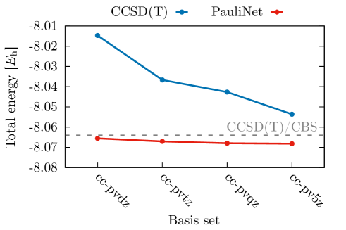
Figure 13: Ground state energy convergence of LiH as a function of the basis set for CCSD(T) and PauliNet. The dashed gray line corresponds to the CCSD(T) energy at the complete basis set limit.

As we can see, CCSD(T) has a very marked dependence on the basis set size. This is a well known shortcoming for all methods defined in Fock space, which suffer from the so-called basis set truncation error. We can estimate what is the CCSD(T) energy at the complete basis set limit by using an extrapolation scheme. Because the Hartree-Fock energy and the correlation energy behave differently as a function of the basis set, we need to extrapolate them separately, using two different extrapolation schemes. For the Hartree-Fock energy, we can use the following formula

$$E_{RHF}^{(X)}=E_{RHF}^{CBS}+A\exp\big{(}-\alpha\sqrt{X}\big{)}$$ (62)

where $A$, $\alpha$ and $E_{RHF}^{CBS}$ are fitting parameters which we can find with the calculations with triple, quadruple and quintuple zeta basis sets, and $X$ is the cardinal number associated to the basis set: 2 for double, 3 for triple, and so forth. Similarly, the correlation energy (note, only the correlation energy without including the Hartree-Fock part) can be extrapolated according to

$$E_{CC}^{CBS}=\frac{X^{B}E_{CC}^{(X)}-Y^{B}E_{CC}^{(Y)}}{X^{B}-Y^{B}}$$ (63)

where $Y=X+1$ and $B$ can be either obtained again by fitting, or set to the value of $B=3$. The plot shown in Figure 13 provides us important insight. First, PauliNet is very insensitive to the choice of basis set. This point was discussed in more detail in the subsection dedicated to ML methods in real space, and is empirically demonstrated here. Second, the correlation energy recovered by PauliNet is more than that from CCSD(T). Considering that PauliNet provides results which are intrinsically at the complete basis set limit regardless from the orbitals used, it implies that the difference between PauliNet and CCSD(T)/CBS is due to missing many-body correlation not captured by the latter. However, as you may have experienced by following this case study, this superb accuracy comes at much more expensive price. A comprehensive investigation of PauliNet with respect to both the basis set limit and the correlation energy limit is presented in [59].

4 Conclusions and Outlook

In this chapter we have seen several unsupervised machine learning approaches to solve the Schrödinger equation. The main advantage is clear, machine learning offers very flexible functional forms which are able to model highly complex many-body correlation effects governing the quantum world. In contrast, traditional quantum chemical methods rely on wavefunction ansätze expressed in a finite number of electronic configurations, which typically span only a fixed and delimited region of an otherwise exponentially large space of functions. While this provides an intuitive framework to describe a quantum state and allows for straightforward optimization schemes, a fixed parametrization significantly constrains the variational freedom of the wavefunction. The risk is to miss important correlation effects outside the range modeled and include instead redundant information of unimportant ones. Machine learning wavefunction ansätze such as Boltzmann machines, Gaussian process states and deep neural networks, start with a different premise. The modeled correlation features are not enforced a priori, instead the wavefunction has complete freedom to take on whatever functional form best describes the quantum state. This has several advantages, for instance there is no more distinction between single-reference and multi-reference, or, in the case of real space approaches, the results do not depend on a basis set anymore. The hard task is then shifted to the optimization of the variational parameters.

For the most part, the ansätze discussed in this chapter are based on highly non-linear maps between input (electronic coordinates or many-body configurations) and output (the associated wavefunction amplitude). This gives rise to two inter-related challenges. On the one hand, the evaluation of expectation values, such as the energy, requires the integration of a high-dimensional function that does not admit an analytical expression. On the other hand, the optimization of the parameters underlying these ansätze is a complicated and computationally demanding minimization problem. The general framework in which these two challenges have been addressed is variational Monte Carlo. This has worked very well to provide compelling evidence that machine learning wavefunction methods are extremely powerful approaches to tackle the quantum many-body problem, but certainly leaves room for improvement for the future. For instance, due to the sharply peaked distribution of wavefunction amplitudes, algorithms that better sample the configuration space (i.e with a higher acceptance rate) are needed; see for example [49]. For methods that can admit analytically tractable expressions, the stochastic framework could also be abandoned in favor of deterministic optimization schemes. This is the case of Gaussian process states, and perhaps highlights one of the advantages of kernel methods over neural networks.

Other interesting developments can be envisioned in the realm of real space approaches. While Fock space methods have overwhelmingly dominated the first wave of machine learning wavefunction, the superb accuracy reached by deep neural networks and their intrinsic independence from a single-particle basis are extremely appealing features. Here, one of the main issues remains the implementation of the antisymmetry property into the wavefunction. Generalized Slater determinants provide a neat solution to this problem, but other routes are possible and being explored [25]. Furthermore, kernel-based methods to model wavefunctions in real space are still missing. We have already seen a glimpse of their potential in the first case study, but it is expected that more concrete examples will appear soon. Furthermore, it is worth exploring the connections between the different representations provided by neural networks and non-parametric models expressed in real space, to those defined in Fock space. As it is often the case, different perspectives on the same method (or representation) can provide additional insight in its mathematical and physical interpretations.

Unsupervised machine learning algorithms are not the only ones that have been developed to model the wavefunction. The SchNOrb neural network has shown an alternative route to deal with the Schrödinger equation. Directly learning the wavefunction is not strictly required, and it might instead be convenient to train a neural network to predict the Hamiltonian representation in a finite basis. In this case, the extensive supervised training required is a computationally demanding task: first, reference data needs to be generated and second, the model needs to learn it comprehensively. However, SchNOrb offers an appealing complementary approach to the unsupervised wavefunction ansätze discussed in this chapter, that has very interesting potential applications, e.g. in molecular dynamics and inverse chemical design.

To conclude, the combination of machine learning and wavefunction theory holds great promise for the future, and constitutes a field that is still in its infancy. Many important developments are thus expected in the future.

References

- [1] Steven R. White “Density matrix formulation for quantum renormalization groups” In Phys. Rev. Lett. 69.19, 1992, pp. 2863–2866 DOI: 10.1103/PhysRevLett.69.2863
- [2] I.E. Lagaris, A. Likas and D.I. Fotiadis “Artificial neural network methods in quantum mechanics” In Comput. Phys. Commun. 104.1-3, 1997, pp. 1–14 DOI: 10.1016/S0010-4655(97)00054-4
- [3] M. Sugawara “Numerical solution of the Schrödinger equation by neural network and genetic algorithm” In Comput. Phys. Commun. 140.3, 2001, pp. 366–380 DOI: 10.1016/S0010-4655(01)00286-7
- [4] Sergei Manzhos and Tucker Carrington “An improved neural network method for solving the Schrödinger equation” In Can. J. Chem. 87.7, 2009, pp. 864–871 DOI: 10.1139/V09-025
- [5] C. Caetano et al. “Using neural networks to solve nonlinear differential equations in atomic and molecular physics” In Int. J. Quantum Chem. 111.12, 2011, pp. 2732–2740 DOI: 10.1002/qua.22572
- [6] Jeremy P. Coe “Machine Learning Configuration Interaction” In J. Chem. Theory Comput. 14.11, 2018, pp. 5739–5749 DOI: 10.1021/acs.jctc.8b00849
- [7] Jacob Townsend and Konstantinos D. Vogiatzis “Data-Driven Acceleration of the Coupled-Cluster Singles and Doubles Iterative Solver” In J. Phys. Chem. Lett. 10.14, 2019, pp. 4129–4135 DOI: 10.1021/acs.jpclett.9b01442
- [8] Giuseppe Carleo and Matthias Troyer “Solving the quantum many-body problem with artificial neural networks” In Science 355.6325, 2017, pp. 602–606 DOI: 10.1126/science.aag2302
- [9] Jing Chen et al. “Equivalence of restricted Boltzmann machines and tensor network states” In Phys. Rev. B 97.8 American Physical Society, 2018, pp. 085104 DOI: 10.1103/PhysRevB.97.085104
- [10] Stephen R. Clark “Unifying neural-network quantum states and correlator product states via tensor networks” In J. Phys. A Math. Theor. 51.13 IOP Publishing, 2018, pp. 135301 DOI: 10.1088/1751-8121/aaaaf2
- [11] Ivan Glasser et al. “Neural-Network Quantum States, String-Bond States, and Chiral Topological States” In Phys. Rev. X 8.1 American Physical Society, 2018, pp. 011006 DOI: 10.1103/PhysRevX.8.011006
- [12] Sujie Li, Feng Pan, Pengfei Zhou and Pan Zhang “Boltzmann machines as two-dimensional tensor networks” In Phys. Rev. B 104.7 American Physical Society, 2021, pp. 075154 DOI: 10.1103/PhysRevB.104.075154
- [13] Yichen Huang and Joel E. Moore “Neural Network Representation of Tensor Network and Chiral States” In Phys. Rev. Lett. 127.17 American Physical Society, 2021, pp. 170601 DOI: 10.1103/PhysRevLett.127.170601
- [14] Dong-Ling Deng, Xiaopeng Li and S. Das Sarma “Quantum Entanglement in Neural Network States” In Phys. Rev. X 7.2, 2017, pp. 021021 DOI: 10.1103/PhysRevX.7.021021
- [15] Xun Gao and Lu-Ming Duan “Efficient representation of quantum many-body states with deep neural networks” In Nat. Commun. 8.1 Springer US, 2017, pp. 662 DOI: 10.1038/s41467-017-00705-2
- [16] Kenny Choo, Giuseppe Carleo, Nicolas Regnault and Titus Neupert “Symmetries and Many-Body Excitations with Neural-Network Quantum States” In Phys. Rev. Lett. 121.16 American Physical Society, 2018, pp. 167204 DOI: 10.1103/PhysRevLett.121.167204
- [17] Tom Vieijra et al. “Restricted Boltzmann Machines for Quantum States with Non-Abelian or Anyonic Symmetries” In Phys. Rev. Lett. 124.9 American Physical Society, 2020, pp. 097201 DOI: 10.1103/PhysRevLett.124.097201
- [18] Yusuke Nomura, Andrew S. Darmawan, Youhei Yamaji and Masatoshi Imada “Restricted Boltzmann machine learning for solving strongly correlated quantum systems” In Phys. Rev. B 96.20, 2017, pp. 205152 DOI: 10.1103/PhysRevB.96.205152
- [19] Rongxin Xia and Sabre Kais “Quantum machine learning for electronic structure calculations” In Nat. Commun. 9.1 Springer US, 2018, pp. 4195 DOI: 10.1038/s41467-018-06598-z
- [20] Giuseppe Carleo, Yusuke Nomura and Masatoshi Imada “Constructing exact representations of quantum many-body systems with deep neural networks” In Nat. Commun. 9.1 Springer US, 2018, pp. 5322 DOI: 10.1038/s41467-018-07520-3
- [21] Zi Cai and Jinguo Liu “Approximating quantum many-body wave functions using artificial neural networks” In Phys. Rev. B 97.3 American Physical Society, 2018, pp. 035116 DOI: 10.1103/PhysRevB.97.035116
- [22] Xiao Liang et al. “Solving frustrated quantum many-particle models with convolutional neural networks” In Phys. Rev. B 98.10 American Physical Society, 2018, pp. 104426 DOI: 10.1103/PhysRevB.98.104426
- [23] Di Luo and Bryan K. Clark “Backflow Transformations via Neural Networks for Quantum Many-Body Wave Functions” In Phys. Rev. Lett. 122.22 American Physical Society, 2019, pp. 226401 DOI: 10.1103/PhysRevLett.122.226401
- [24] Mohamed Hibat-Allah et al. “Recurrent neural network wave functions” In Phys. Rev. Res. 2.2 American Physical Society, 2020, pp. 023358 DOI: 10.1103/PhysRevResearch.2.023358
- [25] Koji Inui, Yasuyuki Kato and Yukitoshi Motome “Determinant-free fermionic wave function using feed-forward neural networks” In Phys. Rev. Res. 3.4 American Physical Society, 2021, pp. 043126 DOI: 10.1103/PhysRevResearch.3.043126
- [26] Kenny Choo, Antonio Mezzacapo and Giuseppe Carleo “Fermionic neural-network states for ab-initio electronic structure” In Nat. Commun. 11.1 Springer US, 2020, pp. 2368 DOI: 10.1038/s41467-020-15724-9
- [27] Peng-Jian Yang, Mahito Sugiyama, Koji Tsuda and Takeshi Yanai “Artificial Neural Networks Applied as Molecular Wave Function Solvers” In J. Chem. Theory Comput. 16.6, 2020, pp. 3513–3529 DOI: 10.1021/acs.jctc.9b01132
- [28] David Pfau, James S. Spencer, Alexander G… Matthews and W… Foulkes “Ab initio solution of the many-electron Schrödinger equation with deep neural networks” In Phys. Rev. Res. 2.3 American Physical Society, 2020, pp. 033429 DOI: 10.1103/PhysRevResearch.2.033429
- [29] Jan Hermann, Zeno Schätzle and Frank Noé “Deep-neural-network solution of the electronic Schrödinger equation” In Nat. Chem. 12.10 Springer US, 2020, pp. 891–897 DOI: 10.1038/s41557-020-0544-y
- [30] Jiequn Han, Linfeng Zhang and Weinan E “Solving many-electron Schrödinger equation using deep neural networks” In J. Comput. Phys. 399 Elsevier Inc., 2019, pp. 108929 DOI: 10.1016/j.jcp.2019.108929
- [31] Andrea Grisafi et al. “Transferable Machine-Learning Model of the Electron Density” In ACS Cent. Sci. 5.1, 2019, pp. 57–64 DOI: 10.1021/acscentsci.8b00551
- [32] Anand Chandrasekaran et al. “Solving the electronic structure problem with machine learning” In npj Comput. Mater. 5.1, 2019, pp. 22 DOI: 10.1038/s41524-019-0162-7
- [33] K.. Schütt et al. “Unifying machine learning and quantum chemistry with a deep neural network for molecular wavefunctions” In Nat. Commun. 10.1 Springer US, 2019, pp. 5024 DOI: 10.1038/s41467-019-12875-2
- [34] M. Gastegger et al. “A deep neural network for molecular wave functions in quasi-atomic minimal basis representation” In J. Chem. Phys. 153.4 AIP Publishing, LLC, 2020, pp. 044123 DOI: 10.1063/5.0012911
- [35] Aldo Glielmo et al. “Gaussian Process States: A data-driven representation of quantum many-body physics” In Phys. Rev. X 10.4 American Physical Society, 2020, pp. 41026 DOI: 10.1103/PhysRevX.10.041026
- [36] Yannic Rath, Aldo Glielmo and George H. Booth “A Bayesian inference framework for compression and prediction of quantum states” In J. Chem. Phys. 153.12 AIP Publishing, LLC, 2020, pp. 124108 DOI: 10.1063/5.0024570
- [37] Julien Toulouse, Roland Assaraf and Cyrus J. Umrigar “Introduction to the Variational and Diffusion Monte Carlo Methods” In Adv. Quantum Chem. 73, 2016, pp. 285–314 DOI: 10.1016/bs.aiq.2015.07.003
- [38] Nicholas Metropolis et al. “Equation of State Calculations by Fast Computing Machines” In J. Chem. Phys. 21.6, 1953, pp. 1087–1092 DOI: 10.1063/1.1699114
- [39] W K Hastings “Monte Carlo sampling methods using Markov chains and their applications” In Biometrika 57.1, 1970, pp. 97–109 DOI: 10.1093/biomet/57.1.97
- [40] Robert Jastrow “Many-Body Problem with Strong Forces” In Phys. Rev. 98 American Physical Society, 1955, pp. 1479–1484 DOI: 10.1103/PhysRev.98.1479
- [41] P. López Ríos et al. “Inhomogeneous backflow transformations in quantum Monte Carlo calculations” In Phys. Rev. E 74.6, 2006, pp. 066701 DOI: 10.1103/PhysRevE.74.066701
- [42] Sandro Sorella, Michele Casula and Dario Rocca “Weak binding between two aromatic rings: Feeling the van der Waals attraction by quantum Monte Carlo methods” In J. Chem. Phys. 127.1, 2007, pp. 014105 DOI: 10.1063/1.2746035
- [43] Nicolas Le Roux and Yoshua Bengio “Representational Power of Restricted Boltzmann Machines and Deep Belief Networks” In Neural Computation 20.6, 2008, pp. 1631–1649 DOI: 10.1162/neco.2008.04-07-510
- [44] Roger G. Melko, Giuseppe Carleo, Juan Carrasquilla and J. Cirac “Restricted Boltzmann machines in quantum physics” In Nat. Phys. 15.9 Springer US, 2019, pp. 887–892 DOI: 10.1038/s41567-019-0545-1
- [45] Yusuke Nomura “Helping restricted Boltzmann machines with quantum-state representation by restoring symmetry” In J. Phys. Condens. Matter 33.17 IOP Publishing, 2021, pp. 174003 DOI: 10.1088/1361-648X/abe268
- [46] Attila Szabó and Claudio Castelnovo “Neural network wave functions and the sign problem” In Phys. Rev. Res. 2.3, 2020, pp. 033075 DOI: 10.1103/PhysRevResearch.2.033075
- [47] Román Orús “Tensor networks for complex quantum systems” In Nat. Rev. Phys. 1.9, 2019, pp. 538–550 DOI: 10.1038/s42254-019-0086-7
- [48] P. Jordan and E. Wigner “Über das Paulische Äquivalenzverbot” In Zeitschrift für Phys. 47.9-10, 1928, pp. 631–651 DOI: 10.1007/BF01331938
- [49] Dian Wu, Riccardo Rossi and Giuseppe Carleo “Unbiased Monte Carlo cluster updates with autoregressive neural networks” In Phys. Rev. Res. 3.4 American Physical Society, 2021, pp. L042024 DOI: 10.1103/PhysRevResearch.3.L042024
- [50] Thomas D. Barrett, Aleksei Malyshev and A.. Lvovsky “Autoregressive neural-network wavefunctions for ab initio quantum chemistry”, 2021, pp. 1–14 arXiv: http://arxiv.org/abs/2109.12606
- [51] Martin C. Gutzwiller “Effect of Correlation on the Ferromagnetism of Transition Metals” In Phys. Rev. Lett. 10 American Physical Society, 1963, pp. 159–162 DOI: 10.1103/PhysRevLett.10.159
- [52] F. Mezzacapo, N. Schuch, M. Boninsegni and J.. Cirac “Ground-state properties of quantum many-body systems: entangled-plaquette states and variational Monte Carlo” In New J. Phys. 11.8 IOP Publishing, 2009, pp. 083026 DOI: 10.1088/1367-2630/11/8/083026
- [53] Hitesh J. Changlani, Jesse M. Kinder, C.. Umrigar and Garnet Kin-Lic Chan “Approximating strongly correlated wave functions with correlator product states” In Phys. Rev. B 80 American Physical Society, 2009, pp. 245116 DOI: 10.1103/PhysRevB.80.245116
- [54] Marcus Hutter “On Representing (Anti)Symmetric Functions”, 2020, pp. 1–22 arXiv: http://arxiv.org/abs/2007.15298
- [55] Kristof T. Schütt et al. “Quantum-chemical insights from deep tensor neural networks” In Nat. Commun. 8.1, 2017, pp. 13890 DOI: 10.1038/ncomms13890
- [56] K.. Schütt et al. “SchNet – A deep learning architecture for molecules and materials” In J. Chem. Phys. 148.24, 2018, pp. 241722 DOI: 10.1063/1.5019779
- [57] Subhas J. Chakravorty et al. “Ground-state correlation energies for atomic ions with 3 to 18 electrons” In Phys. Rev. A 47 American Physical Society, 1993, pp. 3649–3670 DOI: 10.1103/PhysRevA.47.3649
- [58] Shiwei Zhang and Henry Krakauer “Quantum Monte Carlo Method using Phase-Free Random Walks with Slater Determinants” In Phys. Rev. Lett. 90 American Physical Society, 2003, pp. 136401 DOI: 10.1103/PhysRevLett.90.136401
- [59] Z. Schätzle, J. Hermann and F. Noé “Convergence to the fixed-node limit in deep variational Monte Carlo” In J. Chem. Phys. 154.12, 2021, pp. 124108 DOI: 10.1063/5.0032836
- [60] Thom H. Dunning Jr. “Gaussian basis sets for use in correlated molecular calculations. I. The atoms boron through neon and hydrogen” In J. Chem. Phys. 90.2, 1989, pp. 1007–1023 DOI: 10.1063/1.456153