Dynamics of inertial pair coupled via frictional interface

Abstract

Understanding the dynamics of two inertial bodies coupled via a friction interface is essential for a wide range of systems and motion control applications. Coupling terms within the dynamics of an inertial pair connected via a passive frictional contact are non-trivial and have long remained understudied in system communities. This problem is particularly challenging from a point of view of modeling the interaction forces and motion state variables. This paper deals with a generalized motion problem in systems with a free (of additional constraints) friction interface, assuming the classical Coulomb friction with discontinuity at the velocity zero crossing. We formulate the dynamics of motion as the closed-form ordinary differential equations containing the sign operator for mapping both, the Coulomb friction and the switching conditions, and discuss the validity of the model in the generalized force and motion coordinates. The system has one active degree of freedom (the driving body) and one passive degree of freedom (the driven body). We demonstrate the global convergence of trajectories for a free system with no external excitation forces. Then, an illustrative case study is presented for a harmonic oscillator with a frictionally coupled second mass that is not grounded or connected to a fixed frame. This simplified example illustrates a realization and main features of the proposed (general) modeling framework. Some future development and related challenges are discussed at the end of the paper.

I Introducing remarks

Both adhesion/stiction and continuous sliding mechanisms are essential for modeling a frictional interface between moving bodies. Dynamic transitions in friction processes, from the attachment-detachment cycles (see e.g. [1]) to the stick-slip and then continuous sliding (or slipping), see e.g. [2], have been intensively studied on a physical level in tribology and material science. Despite available sophisticated modeling of the frictional interaction of contact surfaces, from nano- to the meso-scale (see e.g. [3] and references therein), a pass over to a lumped parameter modeling of inertial pairs with frictional interfaces is not trivial. In earlier control and system related studies, e.g. [4], kinetic friction usually occurred as an evoked source of damping that acts during the forced motion. In this case, the causal relationship of the kinetic friction usually goes from the motion variables as a source to the friction force variables as a consequence. Accordingly, an externally excited (in other words actuated) relative motion is counteracted by generalized frictional forces arising on a contact interface. This paradigm is entirely independent of the complexity and level of detail of the friction modeling. On the other hand, the contact friction can occur as a joining interface between two inertial bodies that are moving and rubbing against each another. Such a causal relationship would require a generalized frictional force to be the source, and a relative displacement between two bodies of an inertial pair in contact to be the result. In this setting, at least one inertial body is to be regarded as passive and, therefore, to have an unconstrained frictional interface with another (driving) body. This interface should allow for both, conservation of momentum of the moving pair and dissipation of energy with the associated motion damping. To the best of our knowledge, such interactions have been less studied in the past. As such, they deserve attention due to their theoretical and practical relevance for the motion dynamics and control.

A typical example of an application of inertial systems with a frictional interface is a periodic motion of the target body put on a driven surface. Such controlled motion scenarios are exceedingly common in processing and manufacturing on conveyor lines and turntables, material flow of items, surface treatment, preparation of mixed and shaken substances, robot handling of free (i.e. not flanged) objects, and others. More specifically, a dynamic motion trajectory $w(t)$ should reach some region of control tolerance, $\Omega$, surrounding a steady-state periodic orbit (in the relative $(x,\dot{x})$ coordinates) and stay there as illustrated in Fig. 1.

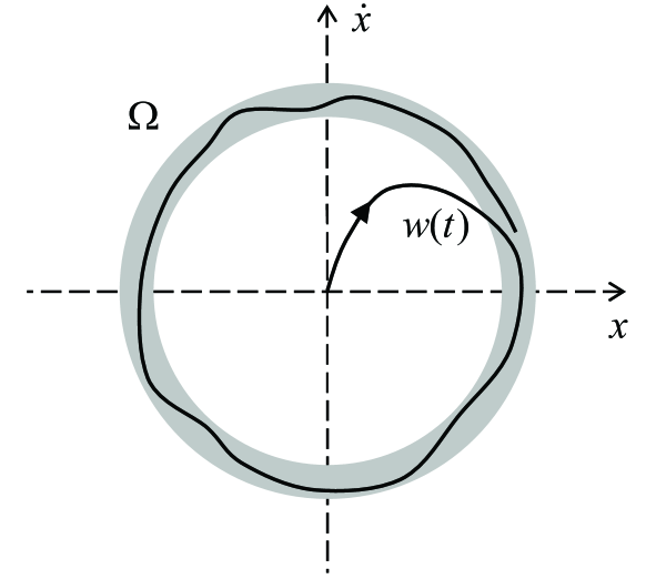
Figure 1: A trajectory $w(t)$ of relative motion of the target body driven via a frictional interface. The ring $\Omega$ indicates the region of control tolerance within the $(x,\dot{x})$ phase plane.

Such control of a periodic motion is sufficiently well understood for dynamics of rigid bodies and even multi-body systems with elasticities, despite the fact that non-trivial reference trajectories and disturbances can pose serious challenges for each particular application. At the same time, to the best of our knowledge, a controlled motion along a target trajectory, or (even simpler) towards a set-point reference, remain largely unexplored for the manipulation of objects which are solely connected via frictional interface.

In the following, we focus on the Coulomb friction (on contact surfaces) [5]. Neither sliding effects of the Prandtl-Tomlinson type (see e.g. [7] for an overview) nor Stribeck effects [8] will be taken into account in order to maintain an adequate complexity of modeling and analysis. We also like to notice that several interesting historical aspects of the development of the Coulomb dry friction law and Stribeck friction curves can be found in e.g. [9] and [10], respectively. Furthermore, smooth breakaway frictional force transitions (see e.g. [11]) at the start of motion, which are characteristic for the so-called presliding friction regime (see e.g. [4, 12]), remain as well outside of our focus. We should also emphasize that dry Coulomb friction would become secondary to our analysis if it only acted as a nonlinear damping and sticking element in an active system with feedback control (see the recent developments in [13]). It gains main attention here once it appears as a dynamic interface between two moving bodies. Finally, we focus on the Coulomb-type frictional interactions in their simplest form, i.e. with a constant speed-independent magnitude and the sign opposed to the relative displacement.

The rest of the paper is organized as follows. In Section II, a dynamical framework of an inertial pair connected via a frictional interface is introduced. Equations (2) – (4) and Fig. 2 provide the most general notation of the overall system dynamics, assuming the contact Coulomb friction with discontinuity at the velocity zero crossing. The convergence analysis of the free system, i.e. without exogenous control action, is delivered in Section III, in terms of the system energy (also Lyapunov) function for the switched and non-switched modes of the relative motion. We exemplify the problem statement and the proposed modeling framework by means of an illustrative case in Section IV. The discussion and relevant points for our future developments are summarized in Section V.

II Dynamics of a pair of bodies with frictional interface

Let us consider a pair of inertial bodies with a frictional interface as shown in Fig. 2.

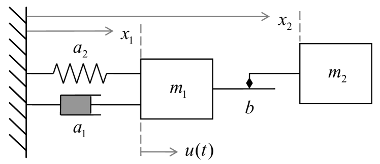
Figure 2: A pair of two inertial bodies with a frictional interface. The first driving inertial body, with the lumped mass $m_{1}$, is connected to the ground. The second driven (i.e. passive) inertial body, with the lumped mass $m_{2}$, is on a flat surface. The moving bodies are connected via frictional interface.

The inertial point-masses $m_{1}$ and $m_{2}$ move in the generalized coordinates $x_{1}$ and $x_{2}$, respectively, having parallel axes. At this point, it does not matter whether a translational or rotational degree of freedom of the relative motion is meant. The single restriction is that a relative motion with only one spatial degree of freedom (DOF) is assumed. A multidimensional case of, for example, relative motion on a flat surface, i.e. with two translational and one rotational DOFs, can be equally elaborated into the proposed modeling framework (see discussion later in Section V), yet it would go beyond the scope of this paper.

The first (actuated) body is connected to the reference ground by a virtual spring with the stiffness $a_{2}$ and a virtual damper with the viscosity coefficient $a_{1}$. Note that both virtual elements can represent (or correspondingly include) mechanical components as well as feedback control terms. For a feedback controlled inertial body, $u(t)$ will then constitute an exogenous input value that can be either a reference motion trajectory, or a generalized disturbing force, or a combination of both. The second inertial body is connected to the first body through a frictional interface which is free of additional constraints. That is, it experiences unrestricted tangential motion (i.e. no mechanical limiters as in a backlash case) and no force constraints other than the normal loading caused by the Coulomb frictional force $f(t)$. In what follows, we assume the classical Coulomb friction with the discontinuity at the velocity zero crossing, see e.g. in [14]. It is worth recalling that the nonlinear Coulomb frictional force represents a rate-independent damping that can be understood in combination with infinite stiffness within the so-called pre-slide friction regime, see [15] for details. While more detailed dynamic friction models attempting to capture the transient side-effects both during presliding and sliding have been studied extensively (see e.g. the seminal papers [4, 12] and the references contained therein), the basic Coulomb law of friction is often sufficient for modeling purposes. In this case, the discontinuous Coulomb friction force opposing the rate of the relative displacement $v$ is captured by $f=b\,\mathrm{sgn}(v)$, where $b$ is the Coulomb friction coefficient, cf. Fig. 2. Further we note that unlike a set-valued sign operator, which is usually used when dealing with the switching or sliding modes (cf. [6]), we use the classical three point valued signum function of a real number $v$, which is defined as

$$\mathrm{sgn}(v)=\left\{\begin{array}[]{ll}1,&\;v>0,\\ 0,&\;v=0,\\ -1,&\;v<0.\\ \end{array}\right.$$ (1)

This allows well-defined solutions at zero differential velocity between two moving bodies, which we will use when introducing the system dynamics.

There are two modes of motion dynamics which should be distinguished depending on whether the relative displacement between the inertial bodies occurs or not: (i) when the second body rests upon the frictional surface (i.e. $\dot{x}_{1}=\dot{x}_{2}$), there is no frictional damping, and the driving body takes on an additional inertial mass, thus, resulting in the total $m_{1}+m_{2}$; (ii) when the second body slides under the action of the frictional force, it impacts the momentum of both bodies which are then either accelerating or decelerating each other. With these assumptions, the equations of motion of the coupled pair shown in Fig. 2 can be written as follows:

$$x_{1}-x_{2} =: z,$$ (2)

$$\Bigl{(}m_{1}+m_{2}\bigl{(}1-\bigl{|}\mathrm{sgn}(\dot{z})\bigr{|}\bigr{)}\Bigr{)}\,\ddot{x}_{1}+a_{1}\dot{x}_{1}+a_{2}x_{1}+b\,\mathrm{sgn}(\dot{z}) = u(t),$$ (3)

$$m_{2}\ddot{x}_{1}\Bigl{(}1-\bigl{|}\mathrm{sgn}(\dot{z})\bigr{|}\Bigr{)}\frac{1}{2}\Bigl{(}1-\mathrm{sgn}\bigl{(}|\ddot{x}_{1}|-bm_{2}^{-1}\bigr{)}\Bigr{)}-m_{2}\ddot{x}_{2}+b\,\mathrm{sgn}(\dot{z}) = 0.$$ (4)

It can be seen that an inclusion of the sign operator (1) in (3) and (4) enables switching directly between the two above-mentioned modes of the system dynamics. In both equations, the switching condition is incorporated in the closed analytic form and, thus, requires neither if-else statements nor case differences, that are otherwise usual when dealing with variable structure hybrid systems. Inclusion of the switching conditions into the dynamic equations (3), (4) comes, therefore, in favor of the their analysis and well-defined solutions of the state trajectories. Note that decoupling of both bodies, correspondingly switching to the mode (ii), is enabled in (4): by the first left-hand-side bracket for a relative displacement between the bodies, i.e. $\dot{z}\neq 0$, and by the second left-hand-side bracket for the case when the stiction condition $|\ddot{x}_{1}|>bm_{2}^{-1}$ is violated.

III Convergence analysis of free system

Let us consider the system (2) – (4) as a switched system. In the following, we assume that there is neither viscous damping term nor control, i.e. $a_{1}=0$, $u=0$. The first assumption is justified by the fact that the viscous damping of the driving body, i.e. $a_{1}\dot{x}_{1}$, is always dissipative and does not directly affect the interaction of the inertial pair. The second assumption of zero control corresponds to free dynamics of the system (2) – (4). Various cases of $u\neq 0$ will be the subject of the future works. With those assumptions, the system (2) – (4) is equivalent to

$$\dot{x}_{1} = v_{1},$$ (5)

$$m_{1}\dot{v}_{1} = -ax_{1}-b\,\mathrm{sign}(v_{1}-v_{2}),$$ (6)

$$m_{2}\dot{v}_{2} = b\,\mathrm{sign}(v_{1}-v_{2}),$$ (7)

where $v_{1}=\dot{x}_{1}$, $v_{2}=\dot{x}_{2}$ and $a=a_{2}>0$. The state space of this system is divided by the switching surface $S=\{(x_{1},v_{1},v_{2}):v_{1}=v_{2}\}$ separating the half-spaces $\Omega_{-}=\{(x_{1},v_{1},v_{2}):v_{1}<v_{2}\}$ and $\Omega_{+}=\{(x_{1},v_{1},v_{2}):v_{1}>v_{2}\}$. The velocity field of (5) – (7) equals

$$\Phi_{-}(x_{1},v_{1},v_{2})=\left(v_{1},-\frac{a}{m_{1}}x_{1}+\frac{b}{m_{1}},-\frac{b}{m_{2}}\right)\quad\text{in}\quad\Omega_{-}$$

and

$$\Phi_{+}(x_{1},v_{1},v_{2})=\left(v_{1},-\frac{a}{m_{1}}x_{1}-\frac{b}{m_{1}},\frac{b}{m_{2}}\right)\quad\text{in}\quad\Omega_{+}$$

with a discontinuity on $S$. Introducing the energy function

$$E=\frac{ax_{1}^{2}}{2}+\frac{m_{1}v_{1}^{2}}{2}+\frac{m_{2}v_{2}^{2}}{2},$$

we observe that

$$\dot{E}=-b|v_{1}-v_{2}|\leqslant 0$$ (8)

along every trajectory of system (5) – (7). Hence, the energy is dissipated on those parts of a trajectory which belong to $\Omega_{-}\cup\Omega_{+}$ and is conserved on the parts which belong to $S$.

In order to describe the switching behavior of trajectories, we consider three parts of $S$:

$$S=S_{-}\cup S_{0}\cup S_{+},$$

where

$$S_{-}=\left\{(x_{1},v_{1},v_{2})\in S:x_{1}<-\frac{b(m_{1}+m_{2})}{am_{2}}\right\},$$

$$S_{0}=\left\{(x_{1},v_{1},v_{2})\in S:|x_{1}|\leqslant\frac{b(m_{1}+m_{2})}{am_{2}}\right\},$$

$$S_{+}=\left\{(x_{1},v_{1},v_{2})\in S:x_{1}>\frac{b(m_{1}+m_{2})}{am_{2}}\right\},$$

and the rays

$$\ell_{-}=\left\{(x_{1},v_{1},v_{2}):x_{1}=-\frac{b(m_{1}+m_{2})}{am_{2}},\ v_{1}=v_{2}<0\right\},$$

$$\ell_{+}=\left\{(x_{1},v_{1},v_{2}):x_{1}=\frac{b(m_{1}+m_{2})}{am_{2}},\ v_{1}=v_{2}>0\right\}$$

that belong to the boundary of the strip $S_{0}$. Since the vector fields $\Phi_{\pm}$ satisfy

$$\Phi_{\pm}\cdot n_{S}<0\ \ \text{on}\ \ S_{+},\quad\Phi_{\pm}\cdot n_{S}>0\ \ \text{on}\ \ S_{-},$$ (9)

$$\Phi_{-}\cdot n_{S}\geq 0,\ \ \Phi_{+}\cdot n_{S}\leqslant 0\ \ \text{on}\ \ S_{0},$$ (10)

where $n_{S}=(0,1,-1)$ is the normal vector to $S$ pointing from $\Omega_{-}$ to $\Omega_{+}$, the part $S_{0}$ of $S$ is the sliding region (or surface), see e.g. [6, 16, 17], consisting of the trajectories and parts thereof known as sliding modes . Each of these trajectories is in the intersection of $S_{0}$ with an ellipsoid $E=E_{0}$ of constant energy. In particular, for

$$E_{0}\leqslant E_{cr}=\frac{b^{2}(m_{1}+m_{2})^{2}}{2am_{2}^{2}},$$

the intersection $\{E=E_{0}\}\cap S_{0}$ is a closed elliptic trajectory, see Fig. 3 (a). On the other hand, for $E_{0}>E_{cr}$ the intersection $\{E=E_{0}\}\cap S_{0}$ consists of two disjoint elliptic arcs, each being a part of a trajectory. One of these trajectories exits $S_{0}$ through the ray $\ell_{-}$ into $\Omega_{+}$, the other through the ray $\ell_{+}$ into $\Omega_{-}$.

(a) (b)

Figure 3: Projection of trajectories of system (5) – (7) onto the switching plane $S$. Parts of the trajectory that belong to the half-spaces $\Omega_{+}$ and $\Omega_{-}$ are shown by blue and red, respectively; parts that belong to the sliding region $S_{0}$ of $S$ are shown in black. (a) A trajectory enters the sliding region $S_{0}$ (the hatched strip) of the switching surface $S$ and merges with one of the elliptic closed trajectories located in $S_{0}$. The energy of the elliptic trajectory satisfies $E<E_{cr}$. (b) A trajectory starting at a point $O_{1}\in\Omega_{+}$ crosses the switching surface $S$ at point $A_{1}\in S_{+}$ and proceeds to the domain $\Omega_{-}$; crosses $S$ again returning to $\Omega_{+}$ at a point $B_{1}\in S_{-}$; enters the sliding region $S_{0}\subset S$ at a point $A_{2}$ and proceeds inside $S_{0}$ to the exit ray $\ell_{+}$; exits $S_{0}$ at a point $C_{1}\in l_{+}$ into the domain $\Omega_{-}$; re-enters $S$ at a point $B_{2}\in S_{0}$, proceeds inside $S_{0}$ to a point $D_{1}\in\ell_{-}$, exits $S_{0}$ through $D_{1}$ to the domain $\Omega_{+}$, re-enters $S_{0}$ at a point $A_{3}$ and proceeds inside $S_{0}$ to a point $O_{2}$. When continued, this trajectory converges asymptotically to the largest elliptic trajectory, which has the energy $E_{cr}$.

Since $\dot{v}_{2}=-b/m_{2}<0$ in $\Omega_{-}$ and $\dot{v}_{2}=b/m_{2}>0$ in $\Omega_{+}$, eq. (8) implies that every trajectory has infinitely many intersections with the switching plane $S$. From (9) it follows that any trajectory from $\Omega_{-}$ either enters the sliding region $S_{0}$ of $S$ and proceeds as described above or intersects $S$ at a point $p\in S_{-}$ transversally (i.e. the intersection point is isolated) and proceeds to $\Omega_{+}$. Similarly, any trajectory from $\Omega_{+}$ either enters the sliding region $S_{0}$ or proceeds to $\Omega_{-}$ transversally through the part $S_{+}$ of $S$, see Fig. 3 (b).

Due to these considerations, eqs. (8), (9) imply that any trajectory of system (5) – (7) either merges with one of the elliptic periodic trajectories (sliding modes) $\{E=E_{0}\}\cap S_{0}$ with $E_{0}\leqslant E_{cr}$ in finite time or converges to the largest of the elliptic trajectories, $\{E=E_{cr}\}\cap S_{0}$, asymptotically. In the latter scenario, there is a sequence of times $t_{1}<\tau_{1}<t_{2}<\tau_{2}<\cdots$ such that

$$\tau_{k}-t_{k}\to\pi\sqrt{\frac{m_{1}+m_{2}}{a}},\quad t_{k+1}-\tau_{k}\to 0$$

as $k\to\infty$ and the trajectory belongs to the sliding region $S_{0}$ during each time interval $[t_{k},\tau_{k}]$, i.e. the trajectory leaves $S_{0}$ only for short intervals of time; further, all the exit points from $S_{0}$ and entry points to $S_{0}$ are located near the end points $(\pm b(m_{1}+m_{2})/(am_{2}),0,0)$ of the rays $\ell_{\pm}$. Also, equation (8) implies that $x_{1}-x_{2}\to const$ for any trajectory.

We conclude that the set of periodic trajectories $\{E=E_{0}\}\cap S_{0}$ with $E_{0}\leqslant E_{cr}$ (including the equilibrium at the origin) is globally asymptotically stable. In particular, one can show that any trajectory starting from $S_{0}$ with energy $E_{0}$, which is slightly higher than $E_{cr}$, converges to the periodic trajectory $\{E=E_{cr}\}\cap S_{0}$ without merging with it. This convergence is slow, slower than exponential. In particular, the energy of such solutions satisfies $c_{1}(E(0))/t\leq E(t)-E_{cr}\leq c_{2}(E(0))/t$ with $0<c_{1}(E(0))<c_{2}(E(0))$.

It is further worth noting, that when a relatively small viscous friction is present, the switching dynamics is similar but the trajectories inside the sliding region spiral towards the equilibrium at the origin, which is globally stable in this case. The counterpart of eq. (8) reads $\dot{E}=-b|v_{1}-v_{2}|-a_{1}v_{1}^{2}$.

IV Illustrative case study

IV-A Example system

The proposed dynamic framework (2) – (4) is further elucidated by the following simplified case study. We assume both unit masses, and the coefficients of the linear sub-dynamics from (3) are assumed to be $a_{1}=0$ and $a_{2}=200$. This renders the first moving body to be a harmonic oscillator, which has the eigenfrequency of $10$ rad/s when the second body is not sliding and rests upon the first one. We allow for different values of the Coulomb friction coefficient to be $0<b<1$. Assuming a free motion, i.e. $u(t)=0$, the dynamics (3) – (4) reduces to an autonomous system

$$\ddot{x}_{1} = -\Bigl{(}2-\bigl{|}\mathrm{sgn}(\dot{z})\bigr{|}\Bigr{)}^{-1}\Bigl{(}200\,x_{1}+b\,\mathrm{sgn}(\dot{z})\Bigr{)},$$ (11)

$$\ddot{x}_{2} = \Bigl{(}1-\bigl{|}\mathrm{sgn}(\dot{z})\bigr{|}\Bigr{)}\,\ddot{x}_{1}+b\,\mathrm{sgn}(\dot{z}).$$ (12)

Note that (12) does not include the acceleration-dependent switching since the system ensures that $|\ddot{x}_{1}|<bm_{2}^{-1}$, cf. (4). An initial condition $x_{1}\,\vee\,\dot{x}_{1}\neq 0$ ensures a finite energy storage at $t=t_{0}=0$ and, therefore, the onset of the relative motion of the free oscillator. According to (12), the second mass is either synchronized with the first inertial mass and, then, has the same acceleration when sticking, or the second mass is sliding with respect to the first mass and, thus, dissipating energy when $\mathrm{sgn}(\dot{z})\neq 0$. In order to develop the state trajectory solutions, we need to distinguish between these two modes of the relative motion:

$$\left.\begin{array}[]{ll}2\,\ddot{x}_{1}+200\,x_{1}=0\\ \ddot{x}_{2}=\ddot{x}_{1}\\ \end{array}\right\} \hbox{if }\;\mathrm{sgn}(\dot{z})=0,$$ (15)

$$\left.\begin{array}[]{ll}\ddot{x}_{1}+200\,x_{1}=\mp b\\ \ddot{x}_{2}=\pm b\\ \end{array}\right\} \hbox{if }\;\mathrm{sgn}(\dot{z})\neq 0.$$ (18)

When inspecting the switched system dynamics (15), (18), one can see that in the first mode, i.e. (15), the system behaves as a pair of synchronized undamped harmonic oscillators with $x_{1}-x_{2}=\mathrm{const}$ and $\dot{x}_{1}=\dot{x}_{2}$ (i.e. $\dot{z}=0$). On the other hand, the piecewise linear dynamics (18) leads to the damped oscillations of $(x_{1},\dot{x}_{1})$ and, thus, to a synchronization of the orbits of both inertial bodies, i.e. $x_{1}(t)-x_{2}(t)\rightarrow\mathrm{const}$ and $\dot{z}\rightarrow 0$, which is in line with the general results obtained in Section III.

IV-B Numerical results

The following numerical results were obtained for system (11), (12) with the first-order forward Euler solver.

Figure 4 shows the motion trajectories of both inertial bodies in the $(x,\dot{x})$ phase-plane when the Coulomb friction coefficient is set to $b=0.5$. Motion trajectories with an initial value $x_{1}(t_{0})=0.006$ are depicted in the plot (a); the other initial values are zero. One can see that the system (11), (12) starts in the stiction mode (15) and remains in this mode at all times featuring undamped harmonic oscillations with the synchronized orbits $(x_{1},\dot{x}_{1})$ and $(x_{2},\dot{x}_{2})$. On the other hand, when an initial value $\dot{x}_{1}(t_{0})=0.15$ is used, as shown in the plot (b), the system (11), (12) starts in the mode (18), i.e. the bodies are in a relative motion subject to the frictional damping. Further, after a period of time the motion of both bodies synchronizes as $\dot{z}$ converges to zero. This transition to synchronization is illustrated by the next example.

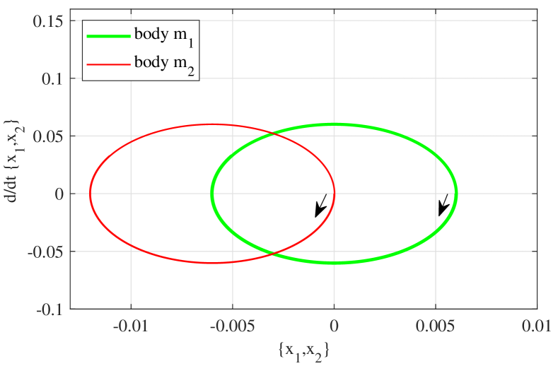
(a) (b)

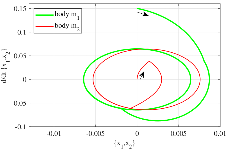
Figure 4: The motion trajectories (in the $(x,\dot{x})$ phase-plane) of the system (11), (12): with the initial $x_{1}(t_{0})=0.006$ in (a), and the initial $\dot{x}_{1}(t_{0})=0.15$ in (b). Other initial values are set equal to zero; the Coulomb friction coefficient is $b=0.5$.

Simulations of the trajectories with an initial value $\dot{x}_{1}(t_{0})=0.15$ for different values of the Coulomb friction coefficient $b=\{0.05,0.2,0.5\}$ are shown in Fig. 5 (b); the panel (a) exemplifies the corresponding time series of $\dot{x}_{1}(t)$ and $\dot{x}_{2}(t)$ for $b=0.05$. One can recognize a constant damping rate of $\dot{x}_{1}(t)$ oscillations due to the Coulomb type energy dissipation. The $\dot{x}_{2}(t)$ trajectory proceeds as a saw-shaped oscillation, owing to the constant acceleration $\ddot{x}_{2}=\pm b$ until both bodies synchronize as $\dot{z}$ approaches zero at the time $t\approx 4.7$ sec. The convergence of the $(z,\dot{z})$ state towards the invariant set $\dot{z}=0$ is clearly visible in Fig. 5 (b) for the three different values of the Coulomb friction coefficient.

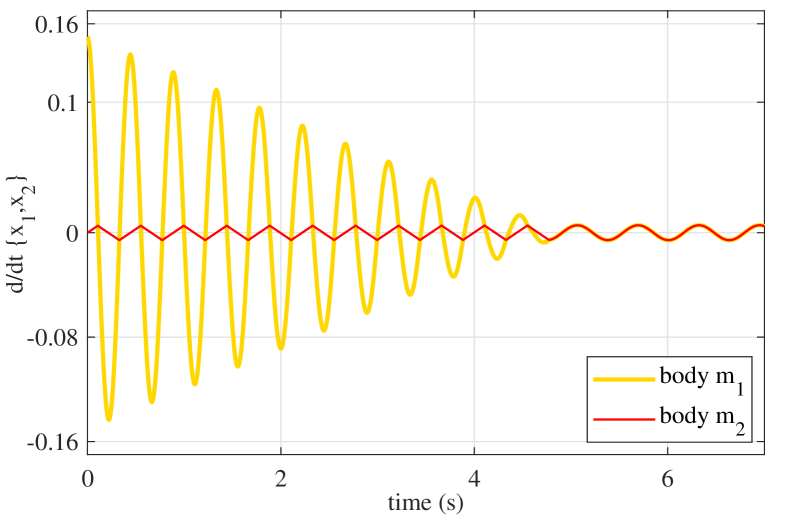
(a) (b)

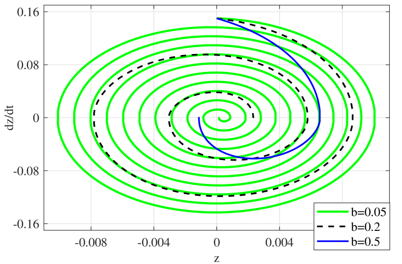
Figure 5: Motion trajectories of system (11), (12) with the initial value $\dot{x}_{1}(t_{0})=0.15$; the other initial values are zero; the time series $\dot{x}_{1}(t)$ versus $\dot{x}_{2}(t)$ for $b=0.05$ in (a), and the $(z,\dot{z})$ phase portrait for $b=\{0.05,0.2,0.5\}$ in (b).

V Discussion

The modeling framework, analysis, and examples described in this paper provide a transparent systems- and control-oriented view of how the friction interface of an inertial pair realizes the coupling of interacting forces and motion variables. One simple insight is that the dry Coulomb friction law can be directly used for defining the switched system dynamics with the two modes of relative motion: (i) the bodies stick to each other; (ii) the bodies slide against each other, cf. (2) – (4) and (15), (18). Moreover, the fact that the moved passive body (cf. Fig. 2) has an unbounded motion space gives an additional insight into how such an underactuated motion system could be controlled when the active body appears as a single (external) energy source, while the motion variables of interest are $(x_{2},\dot{x}_{2})$. A few more discussion points are in order.

• The free system (2) – (4) with $u=0$ is subject to synchronization in the relative $(x_{1},\dot{x}_{1})$ and $(x_{2},\dot{x}_{2})$ coordinates. In particular, for any initial conditions, the global asymptotic convergence $\dot{z}(t)\rightarrow 0$ for $t\rightarrow\infty$ is warranted for all the admissible (i.e. physical) system parameters $m_{1},m_{2},a_{2},b>0$ and $a_{1}\geq 0$.

• Zero convergence of $\dot{z}(t)$ and, therefore, a full synchronization of both moving bodies does not take place in a single dynamic mode, cf. Section III and Fig. 5 (a). A finite time convergence towards a synchronized orbit can precede the following long-term alternation of the stiction (i.e. adhesion) and slipping modes, both in the relative $(z,\dot{z})$ coordinates.

• The viscous damping of the active (driving) body influences the trajectories of the overall system, but has no principal impact on the synchronization mechanism of the moving bodies in a friction-coupled inertial pair. At the same time, a purposefully controlled viscous damping of the active body (cf. damping with $a_{1}$ in Fig. 2) can accelerate the synchronization and be purposefully used for trajectory tracking, cf. Fig. 1.

• We used two alternative descriptions of motion of the coupled inertial pair. As we have seen, the switched system (2) – (4) allows for zero velocity solutions in $\dot{z}$, cf. (1), i.e. adhesion of both moving bodies to each other. On the other hand, the global asymptotic convergence of the free system was shown (cf. Section III) by considering the switched system in Filippov’s sense (cf. (5) – (7)), thus allowing for the sliding modes. In the authors’ opinion, both interpretations of the system switching are possible for the Coulomb friction with a discontinuity. In particular, the sign operator as defined in (1) interprets the adhesion of inertial bodies to each other in a proper physical sense of zero relative velocity. As such, it enables a closed analytic form of the modeling framework (2) – (4).

• While we considered systems with one spatial degree of freedom (in the generalized coordinates), the proposed modeling framework can be further extended to describe motions on a surface. In such a case, one needs to use both orthogonal translational coordinates, e.g. $(x,y)$, and rotational coordinates, e.g. $\varphi$, and introduce an appropriate vector of Coulomb friction coefficients, $\mathbf{b}_{x,y,\varphi}$. Furthermore, this setting requires careful modeling because the coupling terms of friction on a surface are non-trivial from the tribological viewpoint.

• The switched motion system (2) – (4) is underactuated as well as upped-bounded by $\ddot{x}_{1}=\ddot{x}_{2}$, as for the control efforts, cf. (15). The energy- and performance-efficient control methods for the class of friction-coupled dynamical systems (2) – (4) are expected to be challenging. A case study of system (2) – (4) with different types of the application-motivated control, in terms of the dynamic reference signals and external disturbances, will be the subject of the future works. Also, the effect of the time- and state-varying behavior of the frictional interface, i.e. $b(\cdot)$, on the motion dynamics poses an interesting open problem.

References

- [1] H. Zeng, M. Tirrell, and J. Israelachvili, “Limit cycles in dynamic adhesion and friction processes: A discussion,” The Journal of Adhesion, vol. 82, no. 9, pp. 933–943, 2006.
- [2] A. Socoliuc, R. Bennewitz, E. Gnecco, and E. Meyer, “Transition from stick-slip to continuous sliding in atomic friction: entering a new regime of ultralow friction,” Physical review letters, vol. 92, no. 13, p. 134301, 2004.
- [3] A. Vanossi, N. Manini, M. Urbakh, S. Zapperi, and E. Tosatti, “Colloquium: Modeling friction: From nanoscale to mesoscale,” Reviews of Modern Physics, vol. 85, no. 2, p. 529, 2013.
- [4] B. Armstrong-Hélouvry, P. Dupont, and C. C. De Wit, “A survey of models, analysis tools and compensation methods for the control of machines with friction,” Automatica, vol. 30, pp. 1083–1138, 1994.
- [5] C. A. De Coulomb, “Theorie des machines simples, en ayant egard au frottement de leurs parties, et a la roideur des cordages,” Memoire de Mathematique et de Physics de l’academie Royal, pp. 161–342, 1785.
- [6] A. Filippov, “Differential equations with discontinuous right-hand sides,” 1988.
- [7] V. Popov and J. Gray, “Prandtl-Tomlinson model: History and applications in friction, plasticity, and nanotechnologies,” ZAMM - J. of Applied Math. and Mechanics, vol. 92, no. 9, pp. 683–708, 2012.
- [8] R. Stribeck, “Die wesentlichen Eigenschaften der Gleit- und Rollenlager,” VDI-Zeitschrift (in German), vol. 46, no. 36–38, pp. 1341–1348,1432–1438,1463–1470, 1902.
- [9] V. P. Zhuravlev, “On the history of the dry friction law,” Mechanics of solids, vol. 48, no. 4, pp. 364–369, 2013.
- [10] B. Jacobson, “The Stribeck memorial lecture,” Tribology International, vol. 36, no. 11, pp. 781–789, 2003.
- [11] M. Ruderman, “On break-away forces in actuated motion systems with nonlinear friction,” Mechatronics, vol. 44, pp. 1–5, 2017.
- [12] F. Al-Bender and J. Swevers, “Characterization of friction force dynamics,” IEEE Cont. Syst. Mag., vol. 28, no. 6, pp. 64–81, 2008.
- [13] M. Ruderman, “Stick-slip and convergence of feedback-controlled systems with Coulomb friction,” Asian Journal of Control, vol. in print, p. nn, 2021. [Online]. Available: https://doi.org/10.1002/asjc.2718
- [14] V. Popov, Contact mechanics and friction. Springer, 2010.
- [15] M. Ruderman and D. Rachinskii, “Use of Prandtl-Ishlinskii hysteresis operators for Coulomb friction modeling with presliding,” in Journal of Physics: Conference Series, vol. 811, no. 1, 2017, p. 012013.
- [16] C. Edwards and S. Spurgeon, Sliding mode control: theory and applications. CRC Press, 1998.
- [17] Y. Shtessel, C. Edwards, L. Fridman, and A. Levant, Sliding mode control and observation. Springer, 2014.
- [18] S. Adly, H. Attouch, and A. Cabot, “Finite time stabilization of nonlinear oscillators subject to dry friction,” in Nonsmooth mechanics and analysis. Springer, 2006, pp. 289–304.