Neural Adaptive SCEne Tracing (NAScenT)

Abstract

Neural rendering with implicit neural networks has recently emerged as an attractive proposition for scene reconstruction, achieving excellent quality albeit at high computational cost. While the most recent generation of such methods has made progress on the rendering (inference) times, very little progress has been made on improving the reconstruction (training) times.

In this work we present Neural Adaptive Scene Tracing (NAScenT), the first neural rendering method based on directly training a hybrid explicit-implicit neural representation. NAScenT uses a hierarchical octree representation with one neural network per leaf node and combines this representation with a two-stage sampling process that concentrates ray samples where they matter most – near object surfaces. As a result, NAScenT is capable of reconstructing challenging scenes including both large, sparsely populated volumes like UAV captured outdoor environments, as well as small scenes with high geometric complexity. NAScenT outperforms existing neural rendering approaches in terms of both quality and training time.

1 Introduction

In recent years, inverse rendering methods based on implicit neural networks such as NeRF [22] and its variants (e.g. [40], [18], [26], [19], [16], [20], [17]) have garnered a lot of interest in both computer graphics and computer vision. These methods have led to a massive improvement in the quality of 3D reconstruction and re-rendering tasks. Unfortunately, this quality improvement comes at a high computational cost during both training and inference (re-rendering), since the implicit network must be evaluated at millions of points. This shortcoming has so far precluded the use of implicit neural networks for the reconstruction of very large scenes.

In parallel to the development of these neural inverse rendering methods, we have also seen the introduction of neural scene representations [38], [31], [19]. These are not concerned with solving an inverse problem, but instead take an existing image or volume, and compress it into a compact neural network representation. In this space, the ACORN system [19] has shown that hybrid explicit-implicit representations based on hierarchical octree representations can yield a improvements in terms of both the compute time and the quality of fine details in representations of large images and volumes.

Here, we introduce Neural Adaptive Scene Tracing (NAScenT), a hybrid explicit-implicit neural representation that can be trained directly on scene reconstruction tasks (Figure 1). NAScenT uses an octree representation to partition the space into regions according to scene complexity. Each octree node has its own small-scale MLP to represent the node contents. The fully differentiable rendering pipeline employs a ray-based importance sampling scheme in this hierarchical representation, with the importance being determined by an initial node-based splatting approach that maximizes sample reuse across views.

With this approach, NAScenT achieves both high detail accuracy for large scenes, as well as fast training and inference. The adaptive representation works well for a large range of scene types and camera positions, from complex small scale scenes with either full angular coverage or light-field like directional coverage all the way to large sparse volumes that arise in UAV-based capture of large-scale environments.

Specifically, our contributions are: (1) we propose an octree-based neural representation method that represents a scene as an octree with a coordinate-based neural network inside each leaf node and can be trained directly from 2D image data; (2) we also propose an octree structure optimization method that jointly solves multiple neural networks representation and computational resource allocation problems; (3) our representation method can handle challenging cases of large viewpoint change and dynamic camera range cases, e.g. UAV-view terrain scanning.

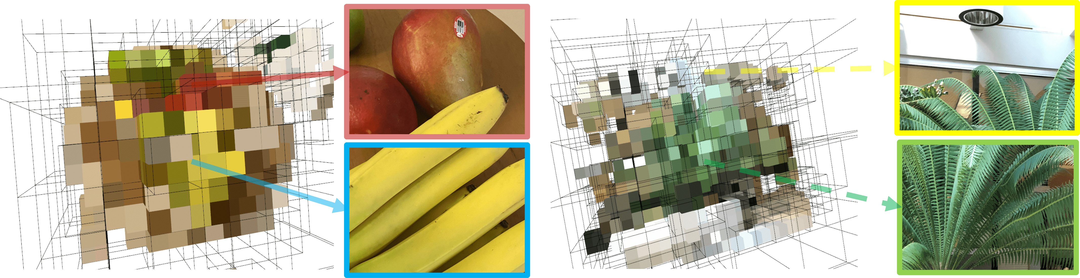
Figure 1: NAScenT jointly optimizes a hybrid explicit-implicit representation consisting of an octree for 3D space partitioning, and structured networks in each active leaf node. Each network maps a spatial coordinate and a direction to a view-independent density and a view-dependent color. NAScenT adaptively allocates more tree nodes to parts of the 3D space with higher scene complexity. Shown here are renderings of novel views, from the fruit and fern datasets.

2 Related Works

3D Scene Reconstruction

is an active research topic in computer graphics. The goal of 3D scene reconstruction is to infer the 3D geometry and texture of a real scene from active measurements [15], passive imaging [1] or by combining both [11]. This task is fundamental in several application fields such as scene understanding, object detection, robot navigation, and industrial inspection. During the last decades, several approaches have been proposed to reconstruct scenes from 2D captured images [28], [44], [1], [12], [7]. In our work, we adopt a multi-view reconstruction approach, where a 3D model of the scene is reconstructed from a set of 2D images taken from known camera viewpoints [30]. The traditional pipeline first recovers camera pose for the multi-views system, and then generates a sparse 3D points distribution of the scene by Structure-from-Motion (SfM) technique. At this stage, a dense scene reconstruction can be obtained by performing multi-view stereo techniques. To enable a photo-realistic viewpoint change, a material type or parametric reflection model can also be specified in the rendering pipeline. Finally, a ray tracing can be performed using a physically-based renderer to simulate the light propagation and the camera imaging process. Recently, neural rendering techniques have been applied with a huge success to the scene reconstruction.

Neural Rendering

techniques have been a resounding success in the computer graphics. They have been applied to achieve realistic rendering of real scenes and improved the view synthesis [8], [33], [22], [23], [29], [5], the relighting and material editing [4], [34], [37], [41], the texture synthesis [24], [27], [6]. Other applications of neural rendering are discussed in the survey [35].

The Neural Radiance Fields (NeRF) work [22] paved the way to a new sub-domain in neural rendering. NeRF and its many adaptations show impressive results in several graphics tasks. However, the large number of samples needed per ray and the requirement to evaluate the network for each sample is a real obstacle for real-time applications. Several strategies have been explored to speed up the neural rendering using NeRF-like networks. These approaches include pruning [18], network factorizations [26], caching [10], use of dynamic data structures [18], [39], and directly learning the integral along a ray [17]. Most of these approaches improve only the rendering performance, but not the training. In this work we specifically target accelerations of the training time by direct training on a hierarchical representation.

3D Scene Representation

is of paramount importance in the reconstruction process. Historically, several ways have been used for the representation of the geometry of the scene, including regular 3D grids of voxels representing discrete occupancy, point clouds, polygon meshes, set of depth maps, or a function of the distance to the closest surface [30]. More recently, several neural representation have been proposed. They can be classified into explicit, implicit and hybrid representations. The explicit methods describe the scene based on a collection of primitives like voxels [32], point clouds [2], meshes [13], or multi-plane images [43], [9]. The rendering using these representations is fast, but their huge requirements in terms of memory, make them challenging to scale.

On the other hand, coordinate-based networks have been introduced to represent scenes in an implicit fashion using neural network [8], [25], [22], [31], [36], [5]. These implicit neural representations leverage a Multi-Layer Perceptron (MLP) to learn a mapping from continuous coordinates to physical properties such as density, field, occupancy or radiance distribution. Despite the impressive results of these representation approaches, they suffer from both a large training time and large rendering time, since the network has to be evaluated for each voxel of the grid. A recent exception is the ACORN system proposed by Martel et al. [19]. It utilizes a hybrid implicit-explicit multi-scale representation in order to combine the computationally efficiency of explicit representations with the memory scalability of implicit approaches. ACORN is also designed to prune empty space in an optimized fashion, and its shows excellent performance in representing fine scale detail on large object domains. However, like several other works [38], [31], ACORN is purely a neural representation, not a neural rendering method. That is, these approaches can be used to compress existing volumes into neural representations, but they cannot in a straightforward way be used for solving scene reconstruction problems.

Our neural representation is inspired by the hierarchical representation of ACORN, but with several crucial adaptations that make NAScenT highly suitable for scene reconstruction tasks.

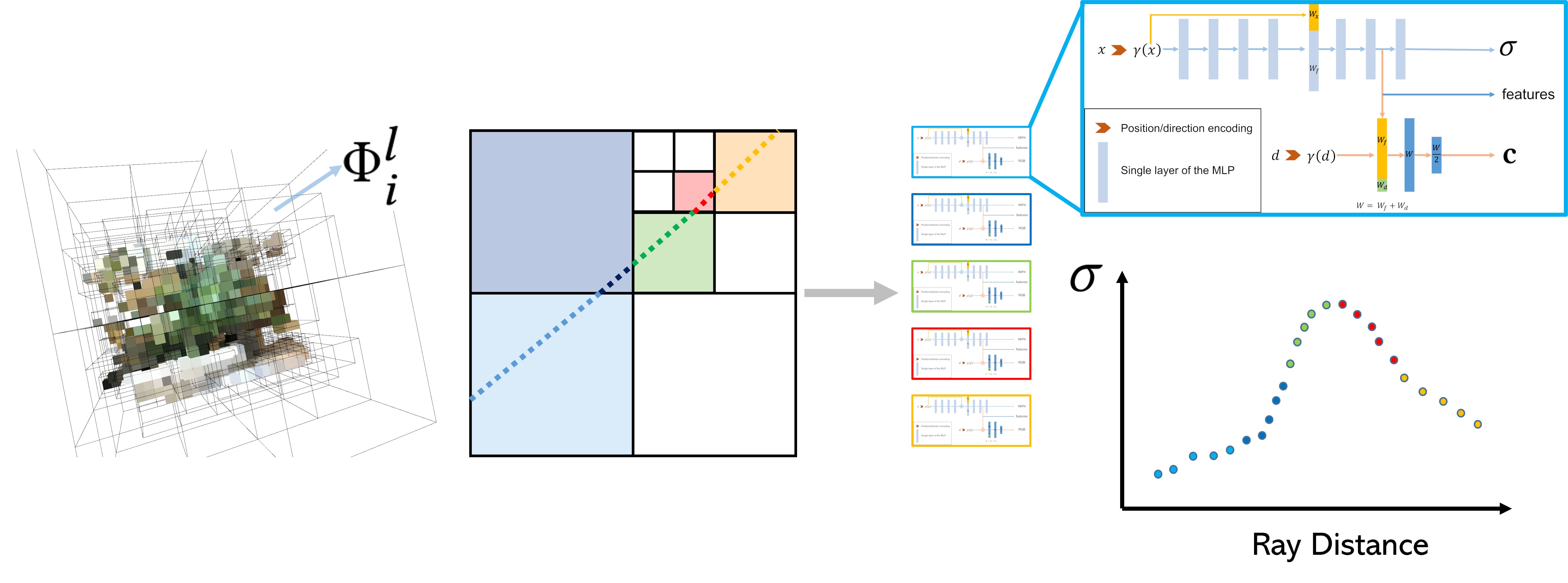
Figure 2: System diagram of NAScenT. The architecture is an explicit-implicit neural representation for the 3D scene, consisting of an octree partitioning of space and a separate lightweight MLP for each leaf node of the octree. The same network architecture and hyper-parameters are used for all octree nodes, which concentrates the model parameters in regions of high complexity. This adaptive representation is combined with an adaptive sampling scheme and differentiable rendering described in the text.

3 Method

NAScenT uses a hybrid explicit-implicit neural representation based on a hierarchical octree data structure (Sec. (3.1)) in which each leaf node has its own neural network, see Fig. (2). This model is evaluated with a two-step sampling approach that concentrates most samples in regions of high geometric complexity as well as near object surfaces (Sec. (3.3)). The samples are then composited front-to-back (Sec. (3.2)) to render images in a differentiable fashion. In this way we can both optimize the neural networks in the leaf nodes as well as adaptively refine the hierarchical model structure (Sec. (3.4), Sec. (3.5)). The details of the individual steps are discussed in the following.

3.1 Hybrid Scene Model

NAScenT uses a hybrid explicit-implicit scene model $\mathcal{M}$, that maps a sample location $\mathbf{x}$ and a viewing direction $\mathbf{d}$ to an RGB color $\mathbf{c}$ and the density or opacity $\sigma$ of the sample:

$$\mathcal{M}=\mathcal{M}_{0}^{0}:(\mathbf{x},\mathbf{d})\rightarrow(\mathbf{c},\sigma).$$ (1)

The explicit part of the representation is somewhat inspired by the hierarchical structure of ACORN [19], however with a number of important differences. Specifically, the model $\mathcal{M}_{i}^{l}$ is recursively defined as either a leaf node represented as a neural network, or a subdivided node with exactly 8 child nodes in standard octree fashion:

$$\mathcal{M}_{i}^{l}(\mathbf{x},\mathbf{d})=\begin{cases}\Phi_{i}^{l}:(\mathbf{x},\mathbf{d})\rightarrow(\mathbf{c},\sigma)&,\text{if leaf node}\\ \bigcup\{\mathcal{M}_{i,1}^{l+1},\dots,\mathcal{M}_{i,8}^{l+1}\}&,\text{else}\end{cases}.$$ (2)

Note that unlike previous hybrid neural representations like ACORN [19], NAScenT does not use a global neural network, but instead individual lightweight networks for the leaf nodes of the octree representation.

The neural networks for each leaf node have the same MLP architecture, depicted in Fig. (2). The network consists of a multi-layered view-independent part and a single view-dependent layer. Note that only the RGB color $\mathbf{c}$ depends on the viewing direction $\mathbf{d}$, while the density $\sigma$ is view independent. This allows us to re-use calculated densities across multiple views (see sampling process below).

The number of layers and neurons per layer in the view-dependent part are hyper parameters, however unless otherwise noted, all experiments in this paper use 8 layers with 64 neurons each. The view dependent layer has 256 neurons. Positional encoding is used for both the position $\mathbf{x}$ and the direction $\mathbf{d}$ with 10 and 4 frequencies, respectively. As the activation function, we use randomized leaky ReLU (RReLU) with a negative lower ($-0.3$) and upper ($-0.1$). Unless otherwise noted, we limit the maximum octree level to 5. The learning rate starts at $5\cdot 10^{-4}$ and is reduced by a factor of 0.1 every 10 epochs.

3.2 Image Formation

Like most recent neural inverse rendering works, NAScenT targets scenes that primarily consist of opaque surfaces. Such scenes are represented well by the front-to-back compositing model introduced by NeRF [22], which we replicate in the following for completeness. Given a set of samples $\{\mathbf{x}_{i}\}_{i}$ along a ray $r$ with direction $\mathbf{d}_{r}$ and the associated color and density values $(\mathbf{c}_{i},\sigma_{i})=\mathcal{M}(\mathbf{x}_{i},\mathbf{d}_{r})$, the corresponding image pixel is given as

$$I(r)=\sum_{i}T_{i}(1-e^{-\sigma_{i}\delta_{i}})\mathbf{c}_{i},\quad\text{where}\quad T_{i}=\exp\left[-\textstyle\sum_{j=1}^{i-1}\sigma_{j}\delta_{j}\right].$$ (3)

Here, $T_{i}$ is the cumulative transparency along the ray segment leading up to sample $i$, and $\delta_{i}$ is a sample weight based on the length of the ray segment between successive samples similar to NeRF [22], but computed independently for each octree node, so that empty or low resolution nodes do not inflate the weight of the first sample in the next node.

Note that this image formation model requires the samples to be ordered front-to-back, since $T_{i}$ in Eqn. (3) requires summation over all samples $j$ closer than $i$. This is straightforward to achieve in non-adaptive representations like NeRF [22] or kiloNeRF [26], but requires extra book keeping efforts in our adaptive, hierarchical approach. Furthermore, any samples located behind an opaque surface will have zero contribution to the pixel value, and will therefore also not contribute to the gradient. Such samples can therefore be culled to reduce the computational burden.

3.3 Two-step Sampling and Ray-tracing

To address these issues we employ a two-step sampling process. First, we use stratified regular sampling in the octree nodes to obtain an estimate of the importance of volume regions to each ray. Then, we apply a ray-based importance sampling scheme along each ray using the information gathered in the first pass.

Stratified node-based sample generation

Considering (3), an important observation is that $t_{i}$, the accumulated transparency along the first part of the ray segment, can act as an effective importance function for the sampling process, along with the hierarchical model structure itself, which refines around regions of high complexity. Furthermore, this cumulative transparency depends only on the density of the samples, but not their color, and the densities independent of ray direction. This makes it possible to re-use samples across different views.

To exploit this observation, we generate samples on stratified grids within each octree leaf node. The number of samples is the same for each leaf node ($64^{3}$ in our implementation), so that the evaluations of the networks $\Phi_{i}^{l}$ can be batched in a straightforward fashion, while the adaptive nature of the octree naturally adjusts the sampling density to the local scene complexity.

In this first sampling stage, we only evaluate the view-independent part of the network, yielding the densities $\sigma_{i}$, which can be re-used for all camera views. Furthermore, since these densities are only used for importance sampling in the second stage, we do not need to generate gradient information for this stage. This makes the process efficient despite the large number of samples generated.

Sample sorting and ray compositing

For each view, the samples generated in this fashion are projected into the image plane, and associated with a pixel and the corresponding ray $r$ (with ray id for each ray). Next, we need to sort the samples belonging to each ray in depth. Instead of solving a large number of small sorting problems, it is more efficient to sort all samples simultaneously. To this end, we assign a global sorting key $z_{g}$ to each sample, which is given as

$$z_{g}=r\cdot z_{\max}+z_{s},$$ (4)

where $z_{s}$ is the sample depth relative to the camera, $z_{\max}$ is the maximum scene depth defines by the user, and $r$ is an integer ray ID. Each sample is associated with the ray corresponding to the pixel it projects to in a nearest-neighbor sense.

Sorting according to this global key will therefore bring all samples into a global order in which successive groups of samples correspond to the same ray, and each group is sorted by depth. The groups are padded to the same maximum length, and then composited in parallel according to Eqn. (3).

Ray-based importance sampling

In the second sampling stage, we generate the actual ray-based sampling pattern that is used for differentiable image rendering. When the sorted stratified samples are given, we estimate the cumulative density distribution (i.e., accumulative sum of $\sigma$) in each block that similar to NeRF’s hierarchical sampling scheme [22] (i.e., stratified sampling based on spatial ray distance), but only evaluate the density distribution within one node. Then, we apply importance sampling to reallocate the samples according to the cumulative density distribution interval (i.e., uniform sampling based on the CDF), assuming that the steep slopes in the CDF indicate true surfaces.

3.4 Optimization of Hybrid Model

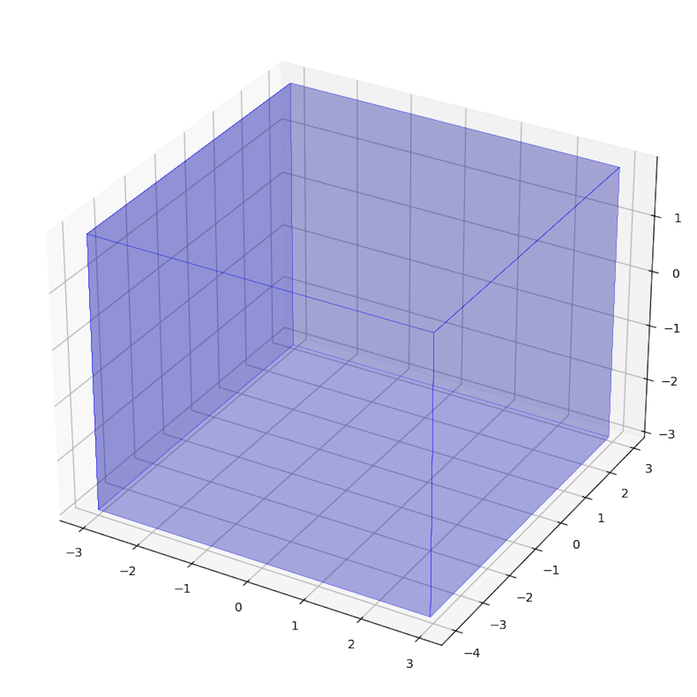
(a) init lv 0

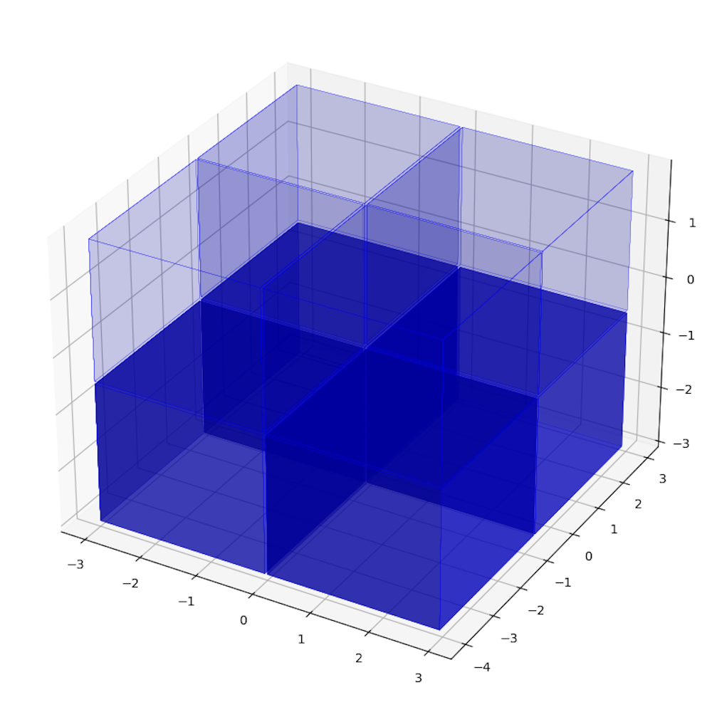
(b) init lv 1

(c) init lv 2

(d) init lv 3

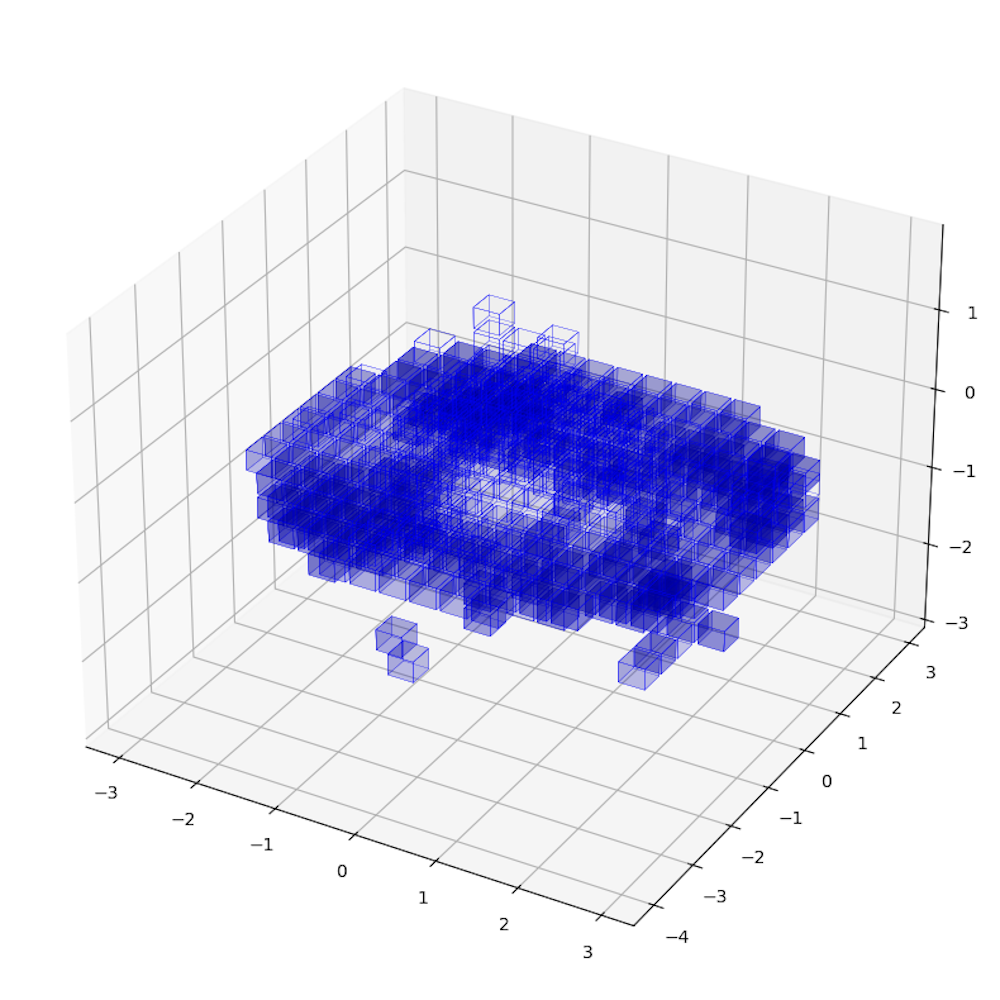
(e) init lv 4

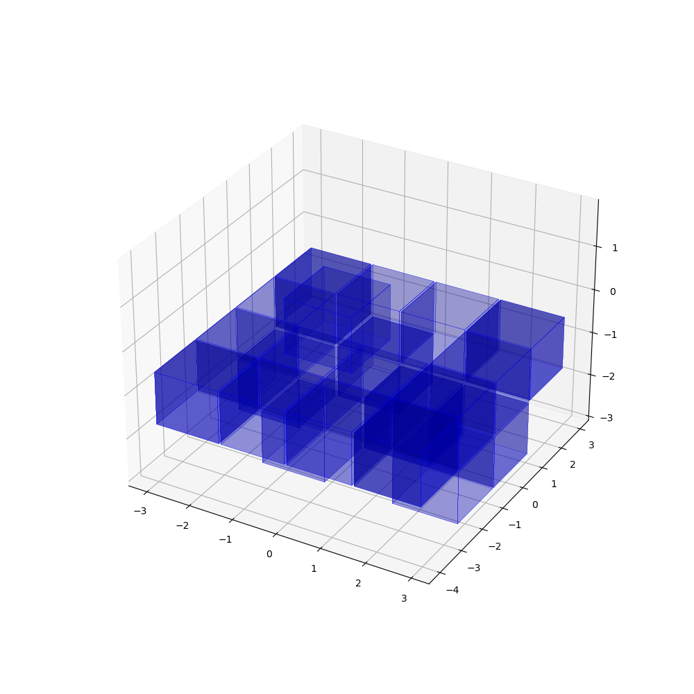
(f) deactivate

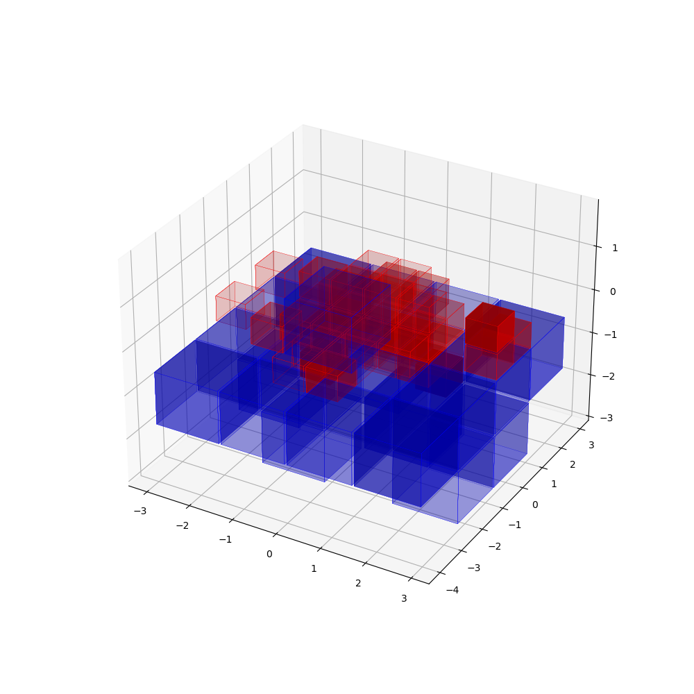
(g) lv 2$\rightarrow$ lv 3

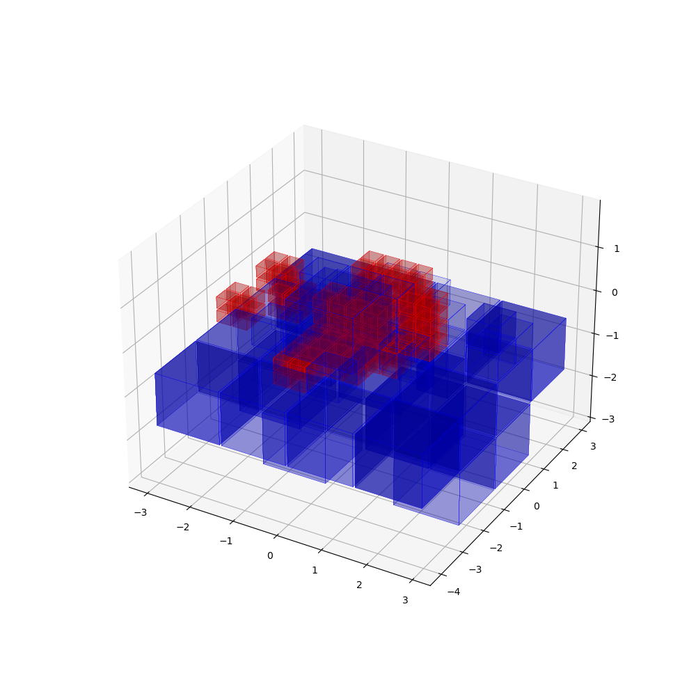
(h) lv 3$\rightarrow$ lv 4

(i) block merge

(j) view

Figure 3: Octree structure update. (a) to (e) show the initial training by using a fully subdivided octree to a given level, with empty nodes culled. (f) only shows active and keep unchanged blocks in level 2, (g) shows block splitting for level 2 to level 3, (h) shows block splitting for level 3 to level 4, (i) shows a block merge to prune the octree for simplification.

The full model $\mathcal{M}$ consists not only of the neural networks in the leaf nodes, but also of the octree structure itself. To optimize this octree structure, we solve an optimization problem with a mixed integer program, similar to the method proposed by ACORN [19]. However, while ACORN is trained directly from a known reference volume, the volume is initially unknown in our inverse rendering setting. We therefore have to devise a different cost function to decide which octree nodes should be subdivided, merged or deactivated.

Specificially, our octree optimization procedure considers both the weighted average density within each node, as well as the aggregated reprojection error within each node. If a weighted average density in a block is less than a threshold (0.01), the block will simply be set to inactive, and will not join the later computation. If a parent node and child node are both active, our algorithm will choose the node with smaller size, i.e. the child node has priority. Please refer to the supplemental materials and the code for more details. Fig. (3) illustrates the evolution of the octree structure from initial levels to full octree optimization stage.

3.5 Model Updates by Pre-training

Every time the octree structure changes, the networks for the old leaf nodes are replaced with new networks for the new leafs. For example, when a leaf node is subdivided, the corresponding network $\Phi_{i}^{l}$ is replaced by eight new networks $\Phi_{i,1}^{l+1},\dots,\Phi_{i,8}^{l+1}$ responsible for the different quadrants. Conversely, when nodes are merged, eight networks at level $l$ get replaced by a single network at level $l-1$.

After such structural changes, we directly pre-train the new network(s) using stratified samples from the previous network(s). This allows the model to quickly return to a similar quality than before the structure change without the need for costly ray-tracing and compositing operations. After this pre-training, the normal ray-tracing-based training resumes.

4 Experiments

For evaluation and both qualitative and quantitative comparison against state-of-the-art methods, we apply our method to several publicly available datasets that have been used by competing methods before, e.g. Synthetic-NeRF [22], LLFF-NeRF [22], DTU Robot Image Data Sets [14]. We also conduct extensive ablation studies for various parameter choices, e.g., sub-network architecture and the number of block levels. In addition to the results in this document, we also refer to the supplemental material for more results.

4.1 UAV-view Terrain Scanning and Reconstruction

In addition to existing standard datasets we also introduce a new UAV-based scene. UAV remote sensing data has usually much sparser view points, with little overlap between neighboring views. Moreover, the standoff distance is often large compared to the scene scale, so that parallax is limited.

This setting is quite challenging for previous neural rendering methods were mainly designed for rendering dense viewpoints with similar camera viewing angles and highly overlapping scene content, and then represent scene by single network [22], [19], [16] or multiple sub-networks [26]. However, a non-adaptive single network structure will have representation capacity problems for training and rendering a large unbounded scene, multiple sub-network [26] will also require a pre-trained single network for better initial performance. Our method contains the optimization of octree structure and sub-network training, thus, the network in each block is only handling representation and reconstruction tasks locally, and could also scale to larger scenes if needed.

Our proposed method is scalable and represents scene content by multiple networks in an octree structure. Therefore the overall representational capacity of the model depends on both the number of octree cells as well as the number of parameters in the networks. Both of these are hyper parameters that we analyze in detail below. However, even very lightweight per-node networks are capable of producing higher quality representations compared to competing approaches.

(a) GT

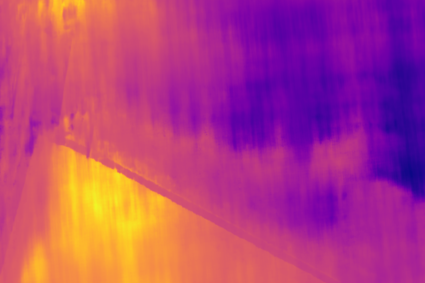
(b) NeRF

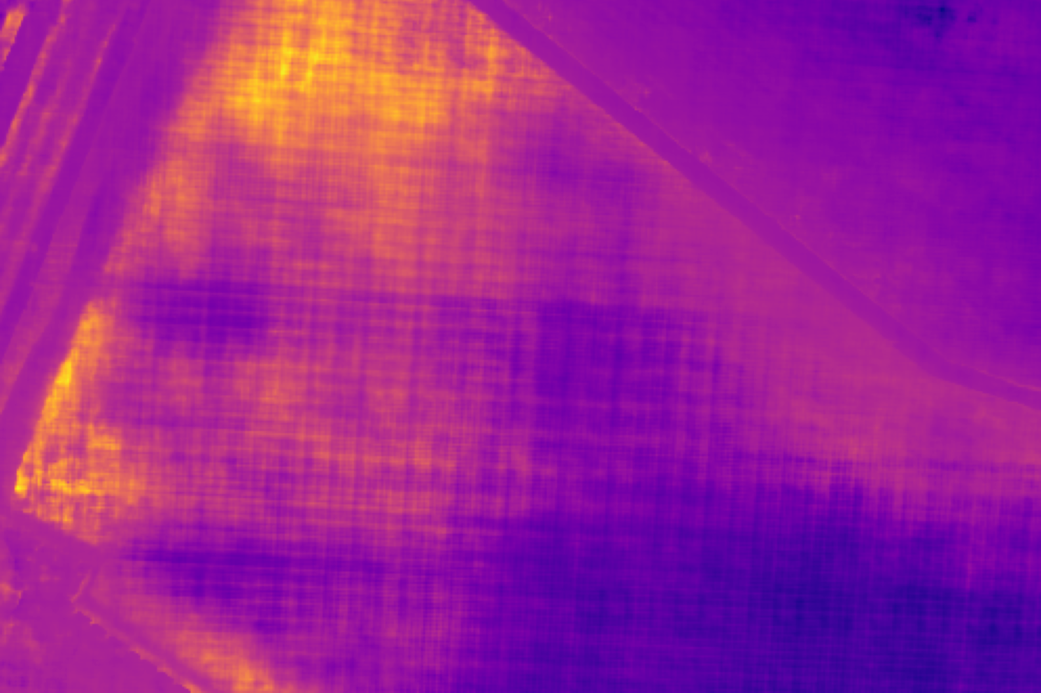
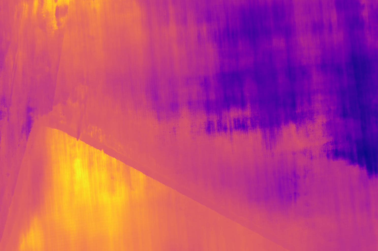
(c) KiloNeRF

(d) MipNeRF

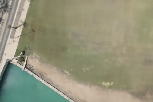
(e) our

Figure 4: Ground scene reconstruction from UAV data (re-rendering from novel view point and false-color rendition of the reconstructed depth map). Note the improved detail in our depth map compared to both NeRF and KiloNeRF, which indicates better leaning of the 3D scene density and also results in better detail preservation in the re-rendering. We compare our method against NeRF [22], KiloNeRF [26], MipNeRF [3].

4.2 Visual Comparison on Public Datasets

We demonstrate the performance of our method by rendering novel views of synthetic and real scene dataset [22] by visualizing novel views in test set as well as the rendered depth map of the scene. Visually, it is difficult to see differences between any of the recent methods for view interpolation – camera positions close to the training positions. However, differences become apparent for view extrapolation, where the novel camera position is far from any of the input cameras. In this document we therefore focus on this view extrapolation scenario for the visual results; the supplemental material has more results.

For comparison methods, we choose those neural rendering methods that can support both sperical and front view scene rendering, including NeRF [22], KiloNeRF [26] and MipNeRF [3].

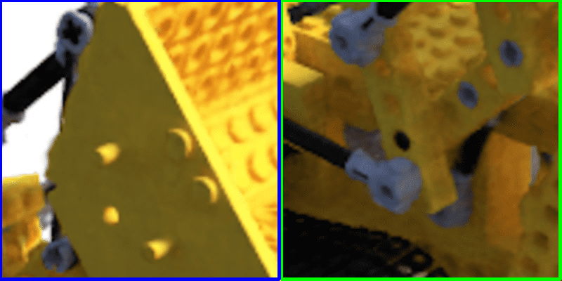
(a) NeRF [22]

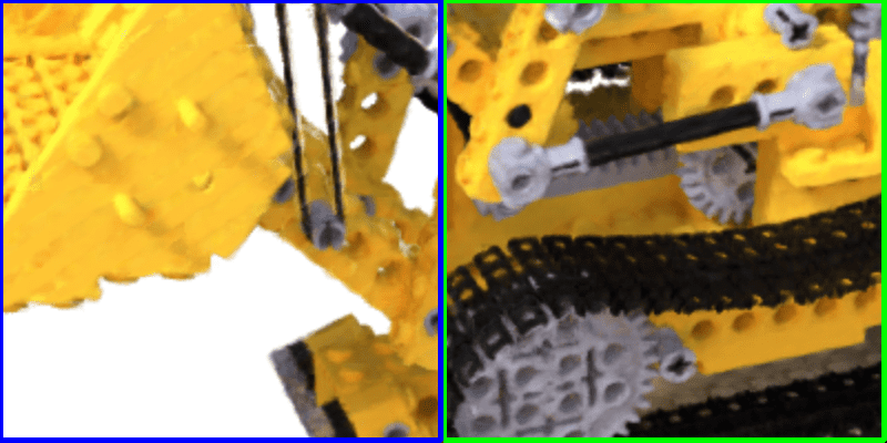
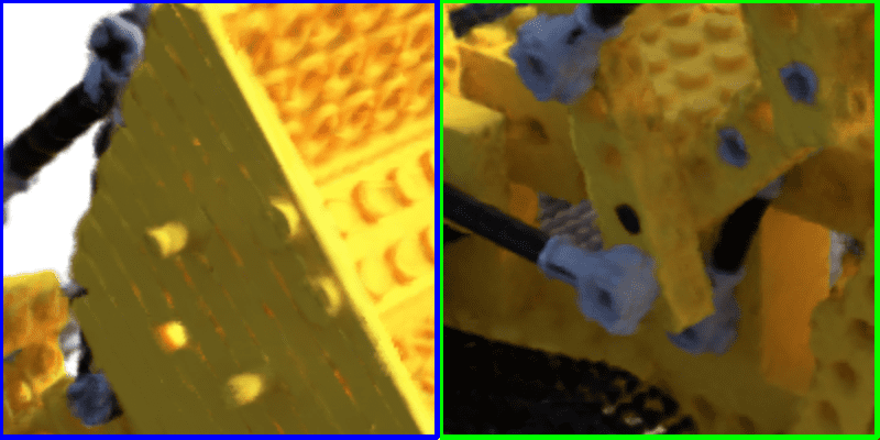
(b) KiloNeRF [26]

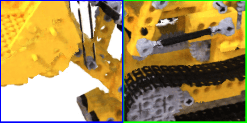
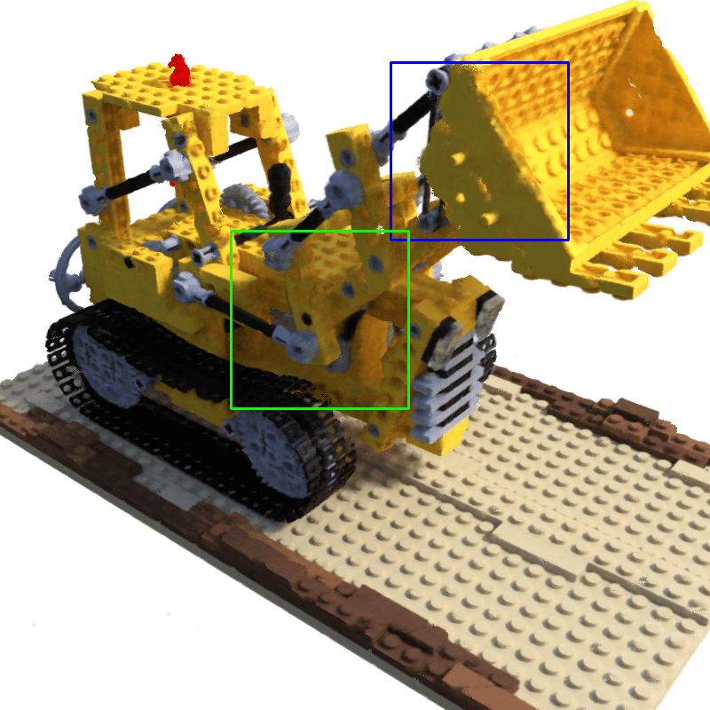
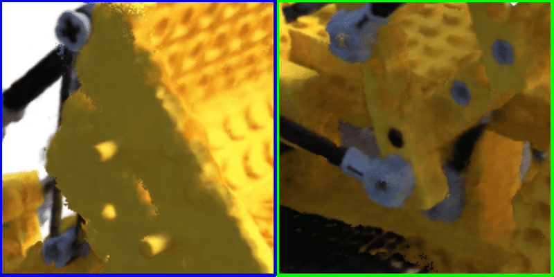
(c) MipNeRF [3]

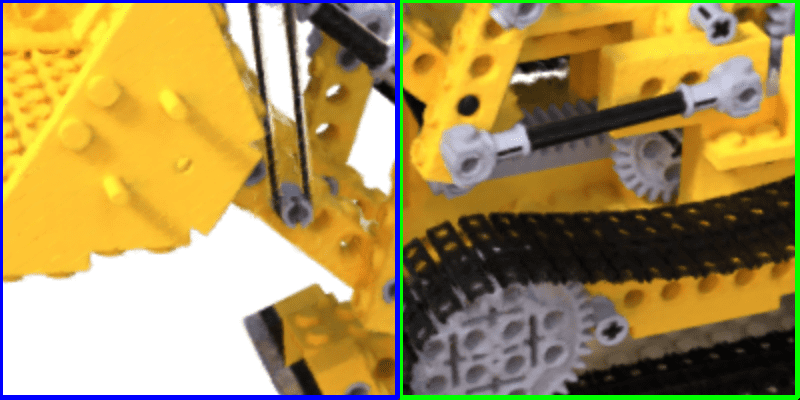
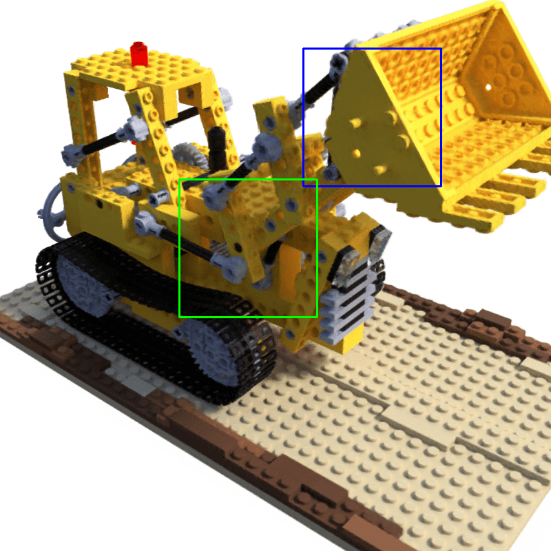
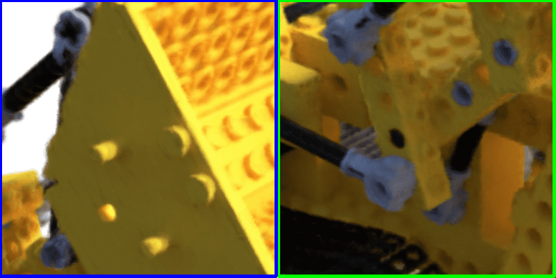
(d) Our

Figure 5: Novel View Comparison on Synthetic Dataset [22]. We render viewpoints from near to far for visualizing viewpoint change and the influence of geometry in rendering.

Synthetic Dataset

Fig. (5) visualizes results for extrapolated viewpoints on the synthetic Lego model. NeRF [22] tend to produce slightly patchy colors in flat areas since incorrect geometry exists in the density field. Also, a single large model is computationally expensive, and therefore limits the number of samples for a ray. KiloNeRF [26] uses NeRF’s model as a teacher to learn a set of small networks for a space partitioning into a regular grid, with the goal of improving the inference (rendering) efficiency and enabling better sampling rates. However, the networks for the individual grid cells are not consistent at cell boundaries, and so light leaks can easily happen in a novel views of the scene, since all the samples along the ray contain zero density for a true surface. Moreover, KiloNeRF also inherits defects from the original NeRF model. MipNeRF has issues at depth discontinuities for these extreme view points, which also indicates that it did not learn an accurate 3D representation. Our method trains the composite model from scratch and enables efficient rendering while avoiding the artifacts of the comparison methods.

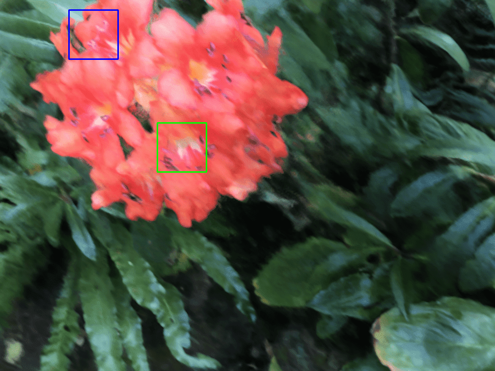
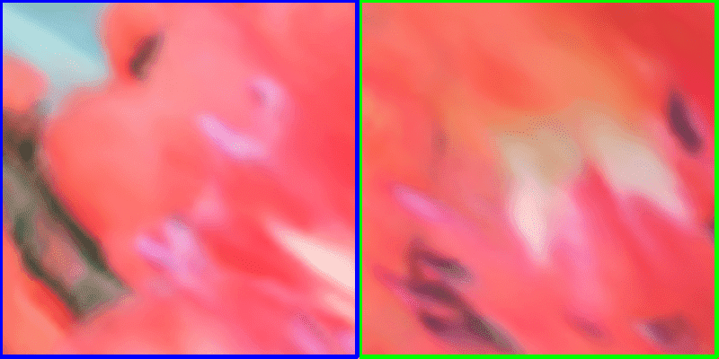
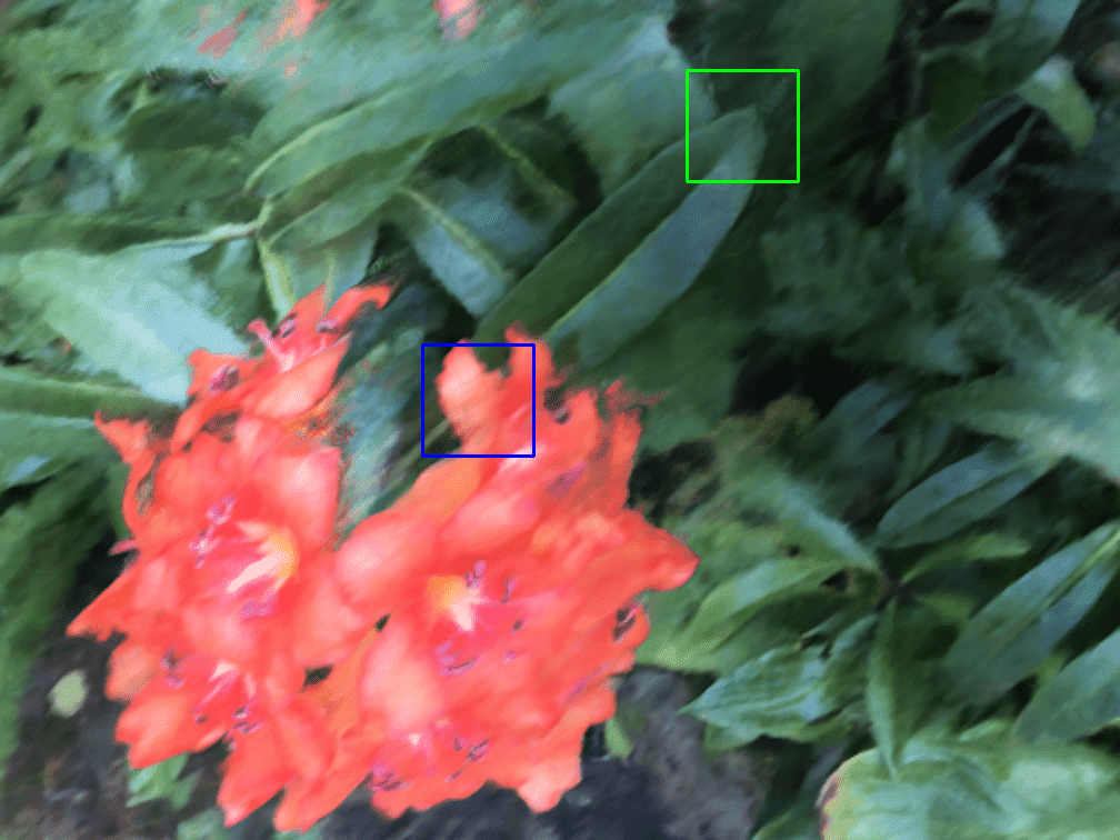
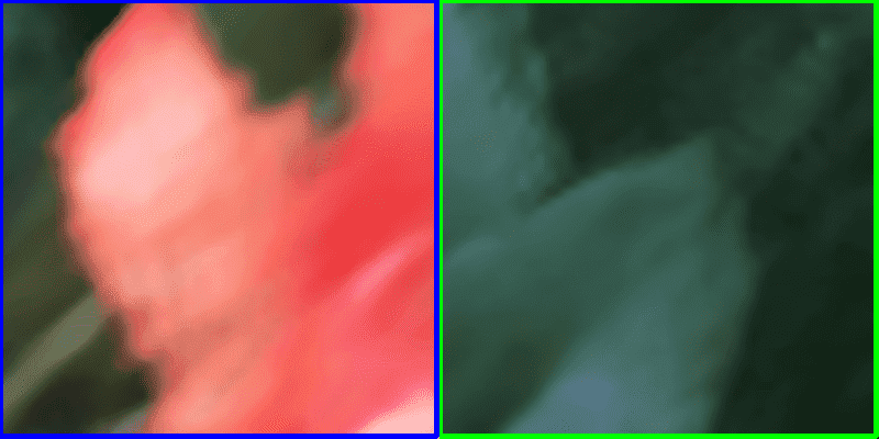
(a) NeRF [22]

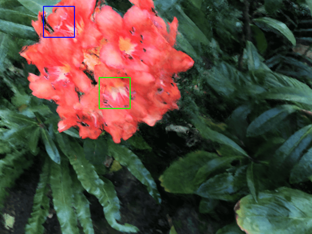
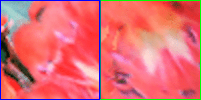
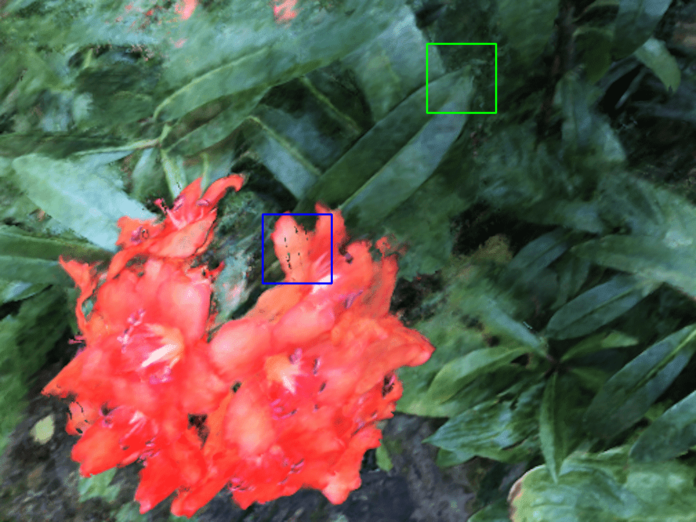
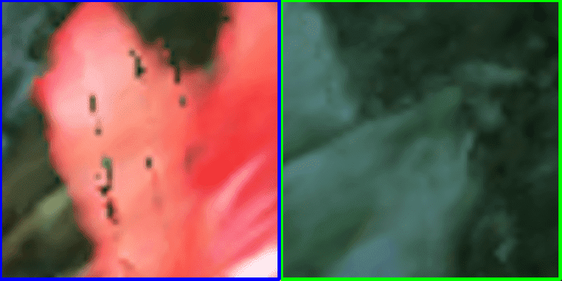
(b) KiloNeRF [26]

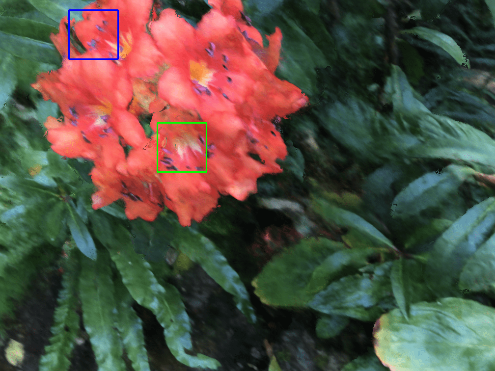
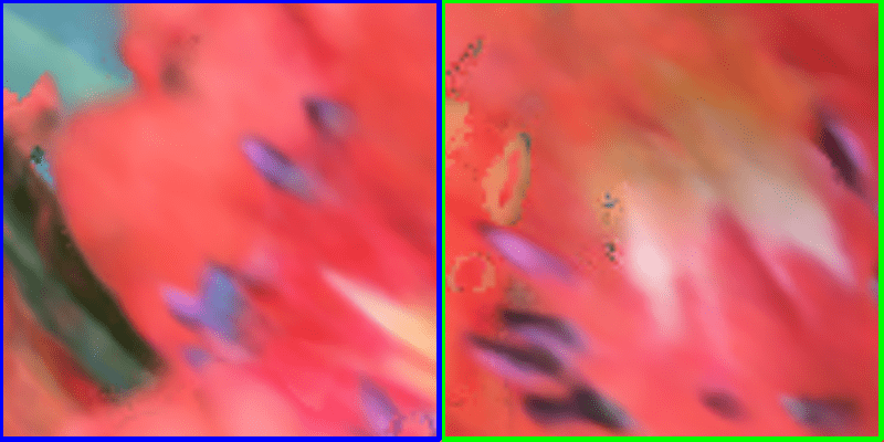
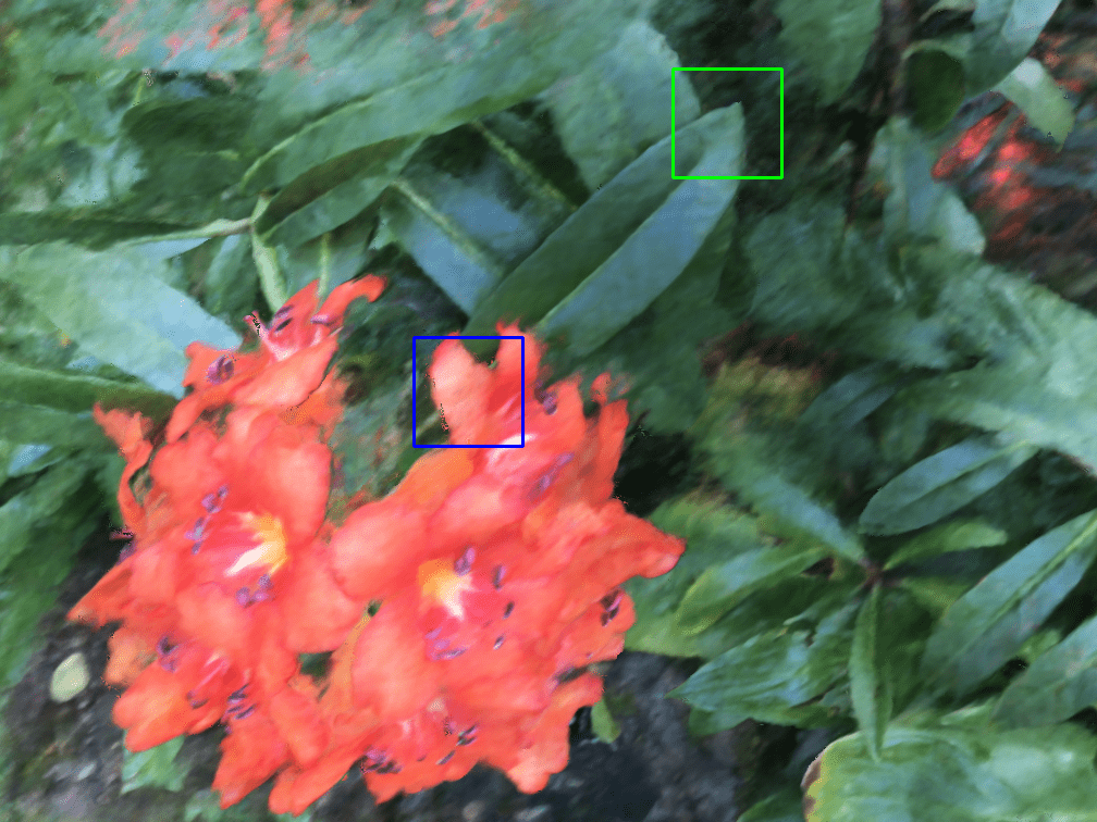
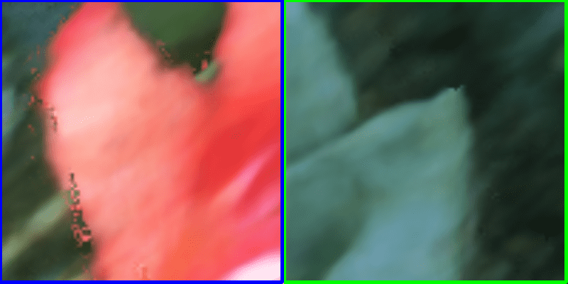
(c) MipNeRF [3]

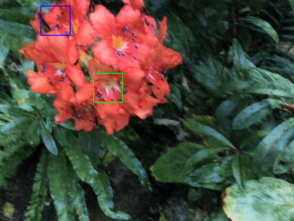
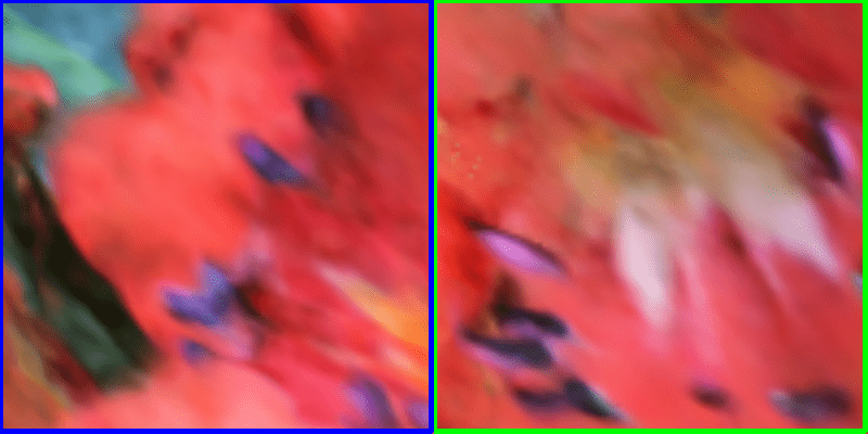
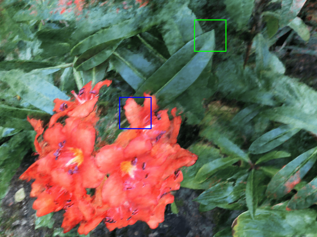
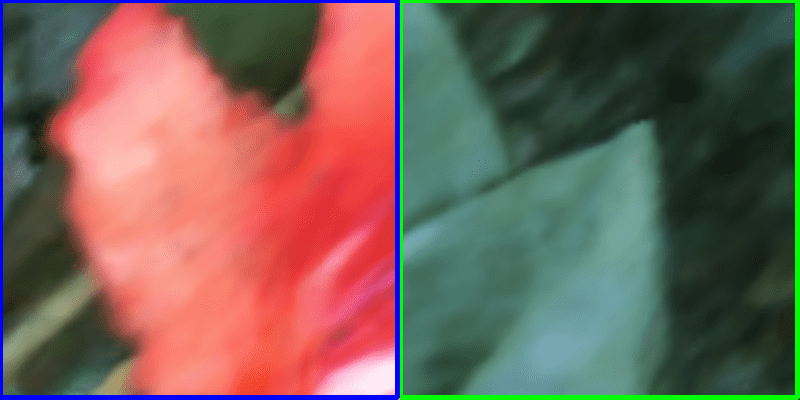
(d) Our

Figure 6: Novel View Comparison on Real Scene Dataset [22]. We render extrapolated viewpoints that far away from view sampling in the training dataset, to show the rendering performance for challenging large viewpoint change.

Real Scene Dataset

Fig. (6) shows an extrapolated viewpoint for a light field dataset, which confirms the findings on the synthetic data. NeRF [22] and KiloNeRF [26] exhibit reduced color accuracy in flower’s androecium (see row 2), while our method can faithfully recover color in fine area due to a better jointly trained geometry and color representation. Moreover, NeRF [22] and KiloNeRF [26] tend to lose shape details in the flower and leaves under strong view point changes. MipNeRF produces sharper results but again also has boundary artifacts at depth discontinuities, indicating an inaccurate density field. On the other hand the octree structure of NAScenT manages to learn a very detailed density field that preserves fine structures over extreme viewpoint changes.

4.3 Quantitative Comparisons

In Tab. (1), we compare our reconstruction results quantitatively against other state-of-the-art works using PSNR, SSIM, and LPIPS [42] as metrics. Note that these comparisons are for the view interpolation scenario since the datasets do not contain comparison views that are far from the training data. The datasets used here are Synthetic-NeRF [22], RealScene-LLFF [21], and the new UAV dataset. Extensive experiments show that our method is highly competitive on all datasets. The most contented dataset is the LLFF dataset, where NAScenT loses to NSVF [18] in terms of PSNR and SSIM, but wins according to LPIPS. LLFF [21] and PixelNeRF are only competitive on the narrow baseline light field data, whereas the other methods show more even performance on all datasets.

Our proposed method excels at the new UAV dataset, since UAV viewpoints have a large view of field, sparse viewpoint and long-range distance, the traditional sampling scheme in NeRF-related methods will waste a large amount of samples in empty space, or hard to sample proper candidates of the ground surface due to limited sampling points along the ray direction. Moreover, NSVF cannot be evaluated on this data because it only reconstructs bounded scenes with extremely high training time in UAV dataset. Our octree-based sampling scheme can achieve uniform sampling inside tree blocks, smaller blocks even have a finer sampling step, in order to enable a better searching scheme for thin objects.

As the ablation studies in the next section demonstrate, we have the ability to further improve the quality by using a more powerful network configuration in each octree node, albeit at a performance cost.

Table 1: Quantitative Evaluation on Synthetic-NeRF[22], RealScene-LLFF[21], UAV dataset.

	Synthetic-NeRF [22]			LLFF [21]			UAV dataset
Method	PSNR$\uparrow$	SSIM$\uparrow$	LPIPS$\downarrow$	PSNR$\uparrow$	SSIM$\uparrow$	LPIPS$\downarrow$	PSNR$\uparrow$	SSIM$\uparrow$	LPIPS$\downarrow$
LLFF	26.05	0.893	0.160	25.03	0.793	0.243	23.70	0.834	0.260
NeRF	31.01	0.947	0.081	27.15	0.828	0.192	24.98	0.853	0.201
PixelNeRF	26.20	0.940	0.080	25.89	0.898	0.187	24.69	0.824	0.201
NSVF	31.75	0.954	0.048	-	-	-	-	-	-
KiloNeRF	30.95	0.937	0.080	26.15	0.828	0.192	25.78	0.864	0.198
Our(W64-D8)	31.85	0.967	0.049	27.79	0.898	0.114	30.48	0.931	0.115
Our(W128-D8)	31.94	0.969	0.048	28.19	0.903	0.113	30.50	0.932	0.113

4.4 Training Efficiency Comaprison

Training time for the Synthetic-NeRF dataset is shown in Table 2. At the default parameter settings detailed in Sec. (3.1), NAScenT has faster training times than the competing methods and competitive rendering times compared to the fastest existing neural rendering methods. Details of the performance/speed trade-off are provided in the next section, and more results can be found in the supplement.

	NeRF	KiloNeRF	MipNeRF	Our(W64D8)	Our(W128D8)
Tot. Time(h)	6.5	18.5	5.3	4.2	11.6

Table 2: Comparison of total training time for Synthetic-NeRF dataset.

4.5 Ablation Study

Network Architecture

We perform an ablation study on the hyper-parameters of the implicit networks for each octree node in Tab. (3). For these use the fruit dataset that contains various zoom-in and zoom-out views to perform ablation study. Note that W and D refer to width and depth of the network. In Fig. (7), we also show novel view rendering results for various sub-networks for a training epochs of 20. Experiments show that the higher approximation power of larger networks improves the image quality, although at significantly higher computational cost. Our default parameters (W64-D8) are on the lower end of the quality scale but provide excellent training and rendering times, and still provide better quality than the comparison methods, as shown above.

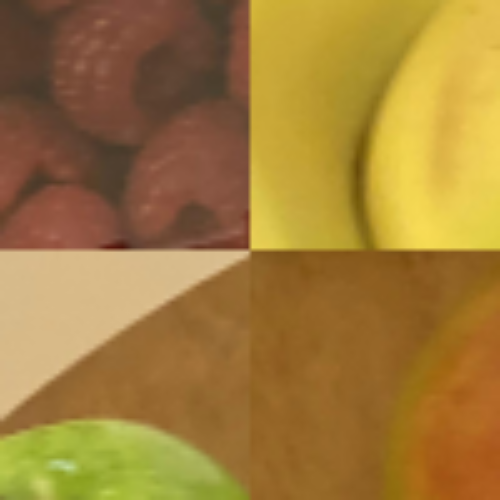
(a) GT

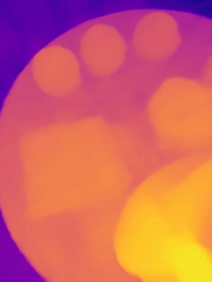
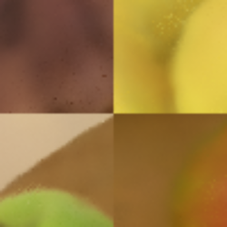
(b) W64D4

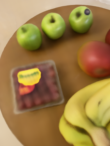
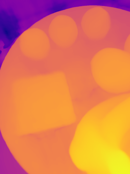
(c) W128D4

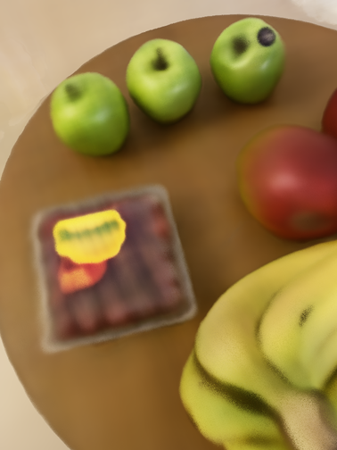
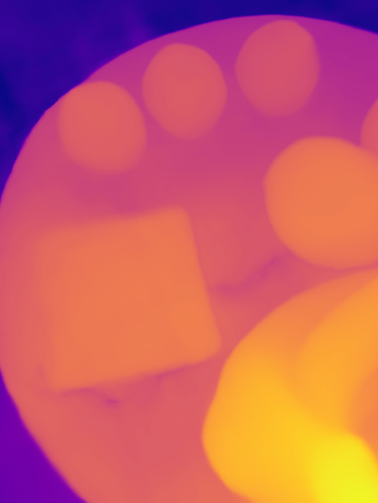
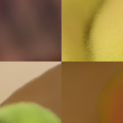
(d) W256D4

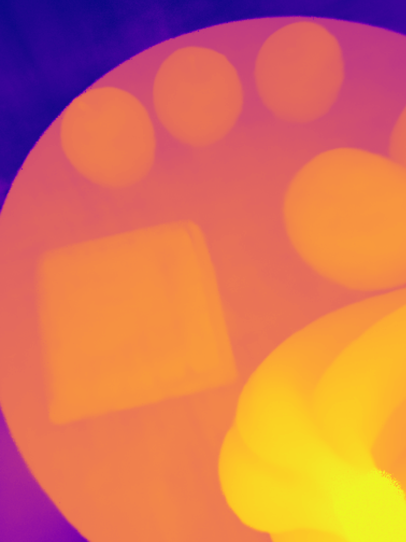
(e) W512D4

(f) W64D8

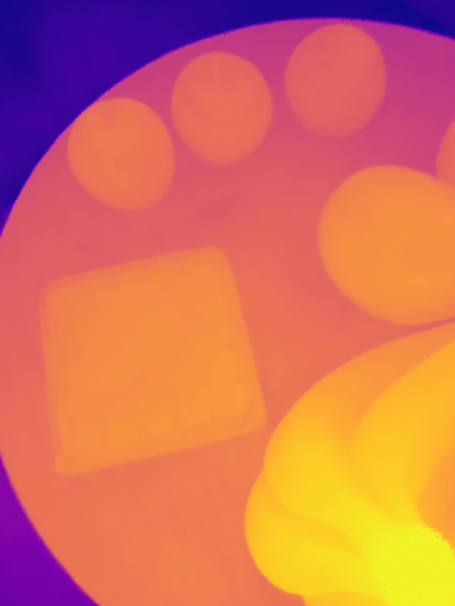
(g) W128D8

(h) W256D8

(i) W512D8

Figure 7: Ablation study for various types of sub-networks architecture. The network width are $\{64,128,256,512\}$, the network depth are $\{4,8\}$.

Table 3: Ablation study on unit network architecture. We fix an optimized octree and replace network architecture in each node to show rendering performance, test on the fruit dataset ($1008\times 756$).

Network	PSNR$\uparrow$	SSIM$\uparrow$	LPIPS$\downarrow$	Train/epoch	Render/frame
W64-D4	26.55	0.921	0.104	4 min	10 s
W64-D8	29.21	0.952	0.093	6 min	12 s
W128-D4	27.85	0.922	0.105	18 min	45 s
W128-D8	29.36	0.953	0.093	20 min	47 s
W256-D4	28.65	0.922	0.105	25 min	55 s
W256-D8	29.89	0.958	0.091	35 min	1.5 min

Table 4: Ablation study on octree levels.

Level (No. $\Phi$)	PSNR$\uparrow$	SSIM$\uparrow$	LPIPS$\downarrow$
level 0 (1)	20.11	0.852	0.220
level 1 (8)	23.42	0.871	0.180
level 2 (64)	27.82	0.941	0.110
level 3 (512)	29.96	0.958	0.091
level 4 (2048)	30.20	0.959	0.080
level all (2633)	30.75	0.961	0.078

Octree Structure

We also compare rendering performance for different granularity of the octree, i.e., the number of octree levels. In general, finer scale octree will have smaller block size and higher representation capacity with higher quantity of sub-networks, therefore, there is a trade-off between the number of sub-networks and the representation capacity. The network architecture is $W64-D8$, and use same dataset as Tab. (3). Tab. (4) shows that a reduction of the octree levels (level 0, 1) has poor performance in rendering, and are thus, and is thus only used for initial training when initializing the system. Level 4 has the best performance with the highest number of networks, but will also lead to the highest computation and storage burden, and is therefore, only active in regions of high complexity. In general, we start training in level 0 or 1 for a warm initialization and initial octree structure, and level 2, 3 are active levels during the main training and rendering process.

5 Conclusions

In this paper, we have presented Neural Adaptive Scene Tracing (NAScenT), a hybrid explicit-implicit neural rendering approach that can be trained directly in the 2D image data. The model representation consists of a hierarchical and adaptive octree structure with a per-node implicit network. We use this model in combination with an optimized two-stage sampling process that maximizes the re-use of view-independent data in order to reduce the number of neural network evaluations. This, together with a strong spatial clustering of the samples near interesting object surfaces, enables improved training times as well as superior results compared to other neural rendering approaches.

The ablation studies show that the quality of the reconstructions can be further improved by utilizing more powerful networks in each node, albeit at significantly increased training and rendering times. We believe this topic merits further investigation. For example one may choose different network hyper parameters for nodes in different regions, based on either a heuristic or neural architecture search. This could further improve the quality while bounding the increase in compute time.

NAScenT is implemented in PyTorch, and the source code and UAV dataset will be made available at the time of publication.

6 Pipeline and Algorithm

In this section, we give a brief introduction for our overall pipleline of algorithms for training and rendering our hierarchical neural networks (NAScenT).

Hierarchical Neural Network Training

Our method takes multiple viewpoint images $I_{gt}$ as input, and outputs the optimized octtree and contained neural networks $\mathcal{M}$. In Alg. (1), $S$ is the set of sampled points by using sampling strategy in Sec. (3.3), and $I(r)$ is rendering RGB value for ray direction $r$. The loss function $\mathcal{L}$ is the photometric loss between rendered pixel values $I$(r) and ground truth values $I_{gt}$(r). The loss is backpropated to each sub-network to update the weights. Every $T_{B}$ rounds of training, the octtree of scene will be updated to adaptively reallocate computational resources to regions with high density and high projected error, and the new sub-networks are directly pre-trained by using stratified samples from the previous sub-networks (see Sec. (3.5) in main).

Input: viewpoint images $I_{gt}$

Output: $\mathcal{M}$

Result: novel views $I$

Initialize $\Phi$, $\mathcal{M}$;

while t $<$ T do

       $S$ = Sampler($\mathcal{M}$)  Sec. (3.3) in main;

       $I$(r) = Render($S$)  Alg. (2);

       loss = $\mathcal{L}$($I$(r), $I_{gt}$(r));

       BackPropagate(loss);

       Step($\Phi$);

       if $t\mod T_{B}=0$ then

             $\mathcal{M}$ = UpdateOctree()  Eqn. (5);

             $\Phi$ = UpdateModel($\Phi$, $\mathcal{M}$)  Sec. (3.5) in main;

            

       end if

      t = t + 1;

      

end while

Algorithm 1 Hierarchical Neural Network Training

Hierachical Neural Network Rendering

Rendering pipeline Alg. (2) takes batches of samples $S$, hierarchical neural networks $\Phi$, and octtree models $\mathcal{M}$ as inputs. Sampling points $S$ are scheduled to corresponding sub-networks $\Phi^{l}_{i}$ by their 3D sample location,. Samples are then evaluates by the respective sub-network $\Phi^{l}_{i}$. To calculate the ordered integral along the ray direction, samples are sorted by Eqn. (4) in main and then composited by Eqn. (3) in main.

Input: 3D scene samples $S$, $\Phi$, $\mathcal{M}$

Output: rendering value $I$

{$S^{l}_{i}$} = Scheduler($S$, $\mathcal{M}$);

$C=\{\}$, $D=\{\}$;

for $\Phi^{l}_{i}$ in $\Phi$ do

       $\mathbf{c}^{B^{l}_{i}}$, $\sigma^{B^{l}_{i}}$ = $\Phi^{l}_{i}(S^{l}_{i})$;

       C.add($\mathbf{c}^{B^{l}_{i}}$); D.add($\sigma^{B^{l}_{i}}$); 

end for

$\{C,D\}$ = SortByZ($\{C,D\}$);  Eqn. (4) in main

$I(r)$ = Composite(C, D);  Eqn. (3) in main

Algorithm 2 Hierarchical Neural Network Rendering

6.1 Importance Sampling

Fig. (8) gives a illustration of the importance sampling in Sec. (3.3).

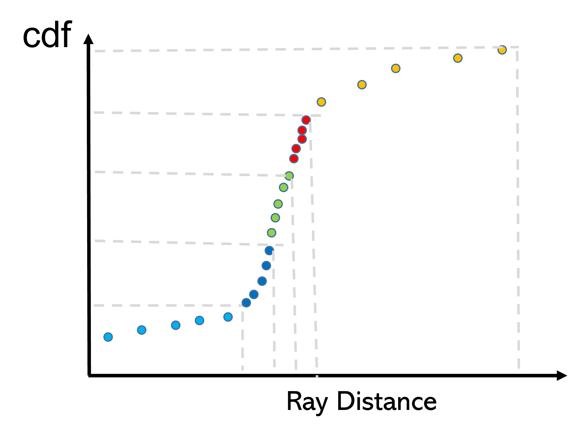
Figure 8: Illustration of sampling scheme that based on cumulative density field.

7 OctTree Update Scheme

In this section, we discuss the details of the octtree update scheme. The intuition of updating structural octtree are (1) avoid time-costly sampling and computation inside empty node, (2) reallocating representation (sub-networks) and computational (number of samples) resource to complex or poorly represented part of the scene.

Our objective mainly contains two parts, $\alpha_{i}$ is weighted average alpha vector of node $i$ of sub-network, which indicates the opaque of node, $\beta_{i}$ is projected rendering error vector of node $i$, since flat or smooth surfaces may converge quickly and be well-trained, while complex or poorly-represented scenes may still need more epochs to obtain better quality. Therefore, the $\beta$ term will explore finer or coarser trees to encourage lower projected rendering error in octtree structure. Our objective is shown as,

$$\min\sum_{i}(1-\alpha^{\intercal}_{i})I_{i}+\beta^{\intercal}_{i}I_{i},\quad\text{s.t.},\begin{cases}I^{\uparrow}_{i}+I^{=}_{i}+I^{\downarrow}_{i}=1,\\ \sum_{i}\frac{1}{N_{c}}I^{\uparrow}_{i}+I^{=}_{i}+N_{c}I^{\downarrow}_{i}\leq N_{B},\\ \end{cases}$$ (5)

where $I_{i}=[I^{\uparrow}_{i},I^{=}_{i},I^{\downarrow}_{i}]^{\intercal}$ are boolean flags of node operations, i.e., merge ($\uparrow$), split ($\downarrow$), and unchanged (=). $\alpha_{i}=[\alpha^{\uparrow}_{i},\alpha^{=}_{i},\alpha^{\downarrow}_{i}]^{\intercal}$ is the weighted average alpha in octree node i for three possible operations, if $\alpha_{i}$ . $\beta_{i}=[\beta^{\uparrow}_{i},\beta^{=}_{i},\beta^{\downarrow}_{i}]^{\intercal}$ is the weighted average projected rendering error respectively. $N_{B}$ is user-defined maximal block in system.

To calculate value $\alpha_{i}$, we first perform stratified sampling from top to bottom in the octree hierarchy and predict the density value for each sample by running the forward rendering network $\Phi(\mathbf{x},\mathbf{d})=(\mathbf{c},\sigma)$, then the $\alpha_{i}^{=}$ for each block by,

$$\begin{cases}\alpha^{=}_{i}=\frac{1}{|S_{i}|}\sum_{\mathbf{x}\in S_{i}}\delta(\mathbf{x}),\\ \alpha^{\uparrow}_{i}=\frac{1}{N_{c}}\alpha^{=}_{\mathcal{P}(i)},\\ \alpha^{\downarrow}_{i}=\sum_{j\in\mathcal{C}(i)}\alpha^{=}_{j},\\ \end{cases}$$ (6)

where $\mathcal{P}$ and $\mathcal{C}$ are query functions for octree parent and child nodes. $S_{i}$ denotes the samples inside an active block.

To calculate $w_{i}$ for different cases, we first evaluate rendering error for each ray $E(\mathbf{r})=\mathcal{L}(I(r),I_{gt}(r))$, and $\mathcal{L}$ is simple function for mean square error.

$$\begin{cases}\beta^{=}_{i}=\frac{1}{|S_{i}|}\sum_{\mathbf{x}\in S_{i}}\frac{w(x)}{W}E(\mathbf{r}),\\ \beta^{\uparrow}_{i}=\frac{1}{N_{c}}\beta^{=}_{\mathcal{P}(i)},\\ \beta^{\downarrow}_{i}=\sum_{j\in\mathcal{C}(i)}\beta^{=}_{j},\\ \end{cases}$$ (7)

where $w(x)$ is the weight in rendering function Eqn. (3) in the main paper (i.e., $T_{i}$) for samples $x\in\mathbf{r}$. $W=\sum_{x\in\mathbf{r}}w(x)$ is the total sum of weights along the ray direction. To optimize Eqn. (5), we use or-tools to solve MIP problems.

8 Additional Comparison and Results

(a) GT

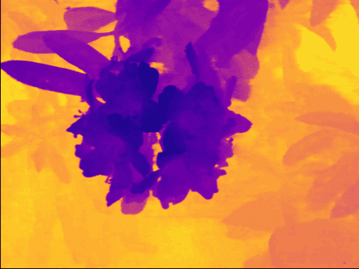
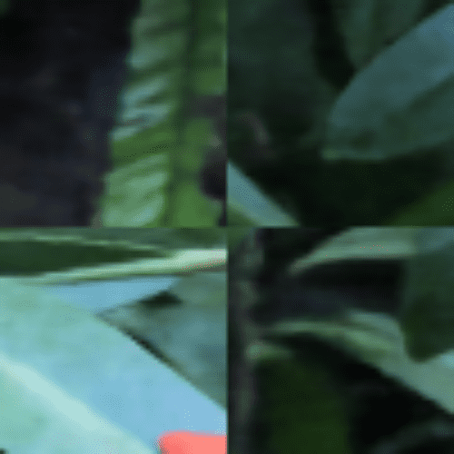
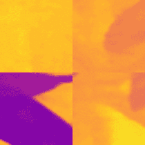
(b) NeRF[22]

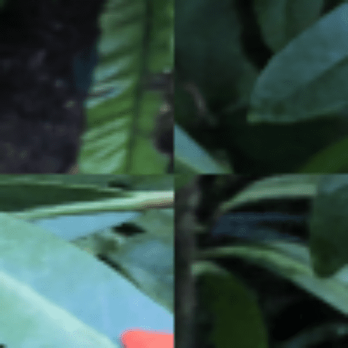
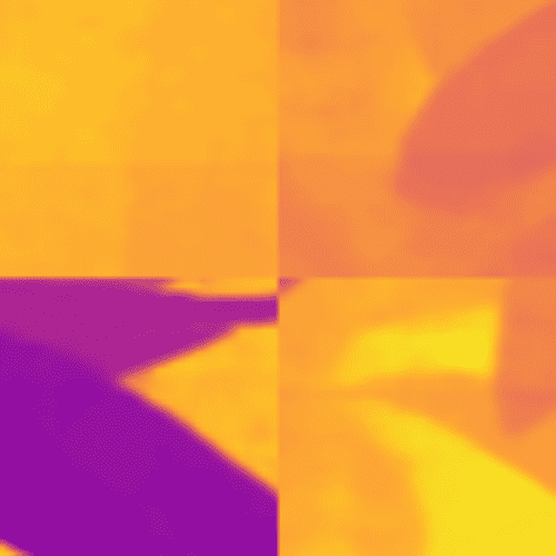
(c) KiloNeRF[26]

(d) Our

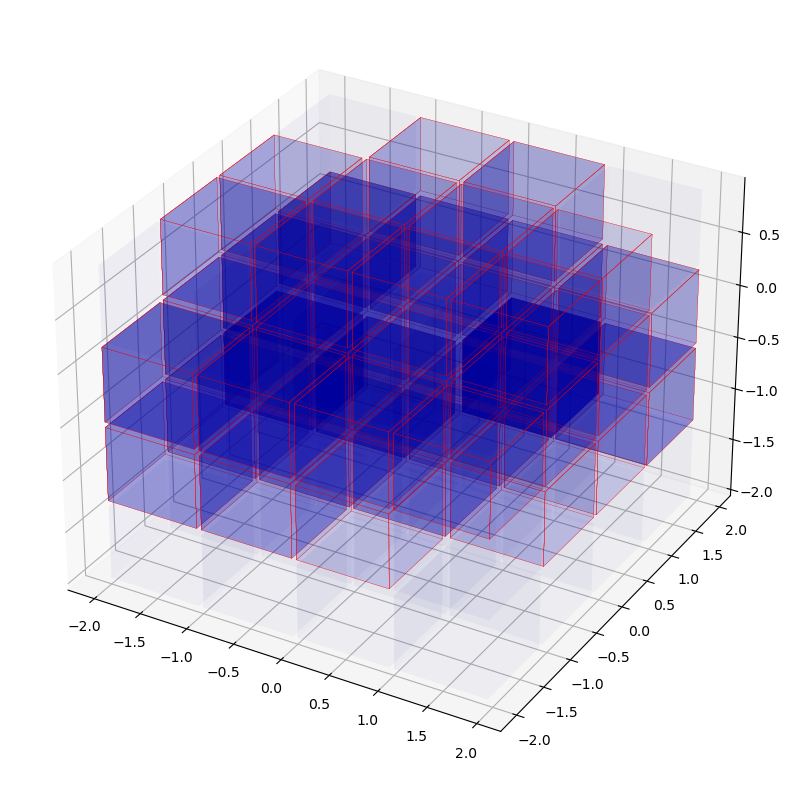
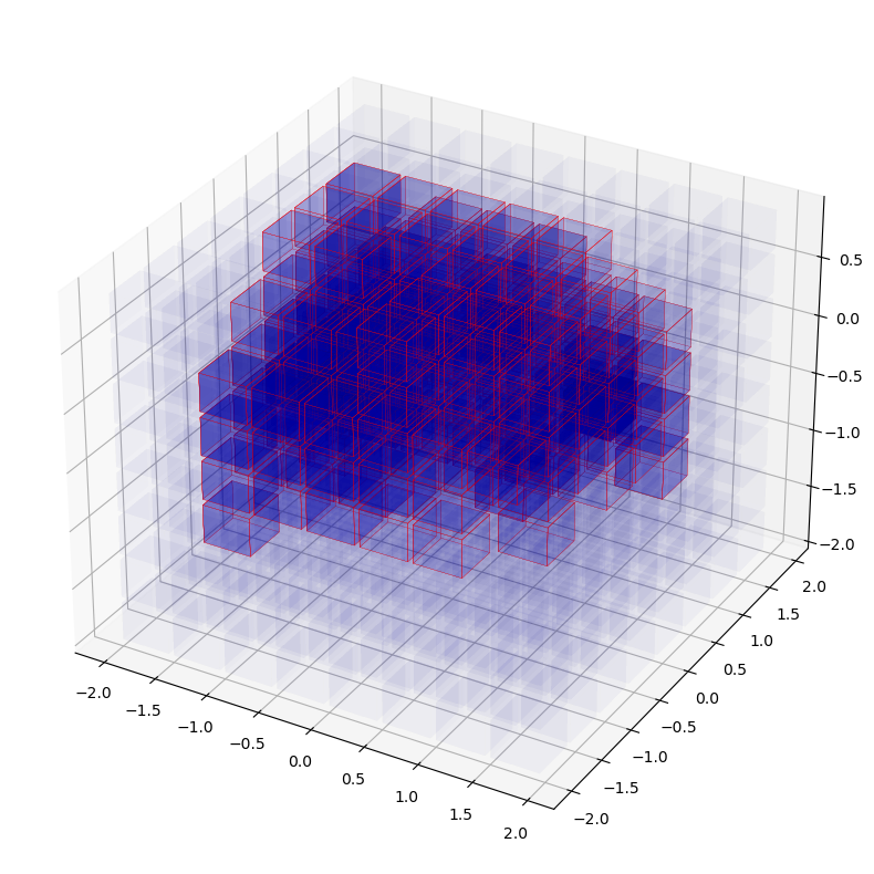
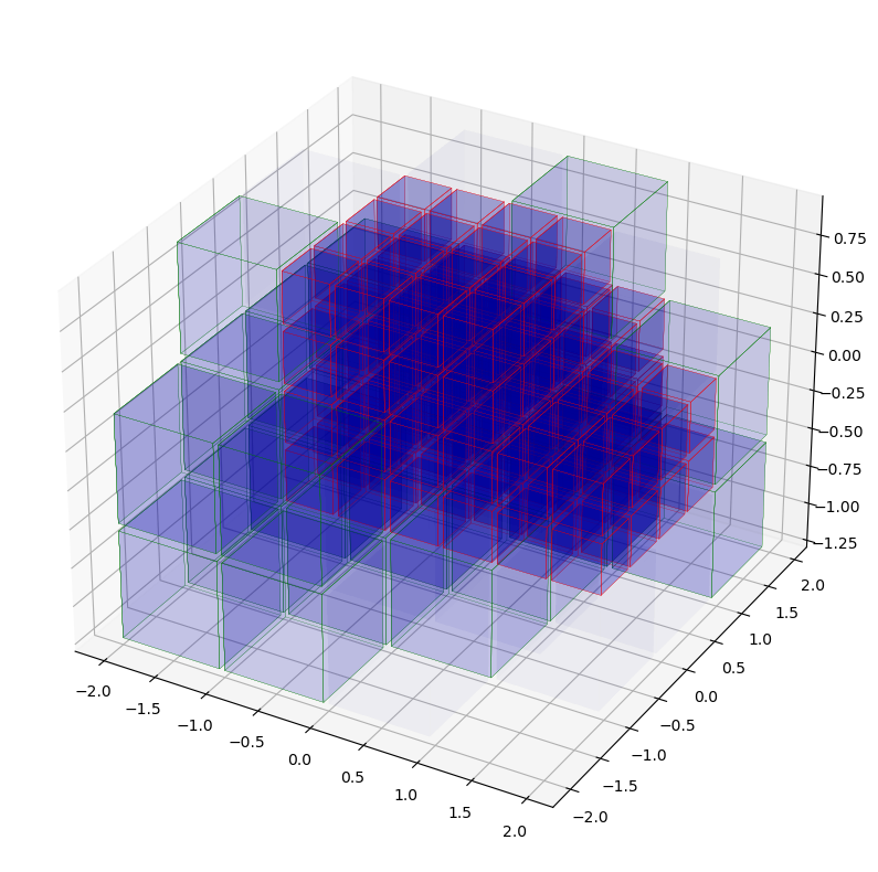
(e) Octree

Figure 9: Visual Comparison on LLFF-NeRF dataset [21].(a) is ground truth view of flower scene with highlighting details. (b)-(d) are the novel view of NeRF [22], KiloNeRF [26] and our methods with highlight details. (e) the visualization of example view and octree optimization process from initial level 2 to level 3, and merge to simple structure to save computational and sampling resource.

In this section, we show extensive comparison in details and results. As discussed in the main text, for views close to the training views all methods produce visually very similar results; differences only become apparent at close inspection and when analyzing depth structure. However, as the results in the main paper show, the differences in the depth estimation amplify the visual quality differences for extrapolated views far from the training data.

Fig. (9) shows visual comparisons of novel view synthesis on real scenes from the LLFF-NeRF dataset [21]. As we can see in the figure, NeRF [22] can miss surfaces with its sampling process so that back surfaces can “shine through”. This is due NeRF’s sampling scheme that applies stratified search for a coarse-level density distribution estimation and then sampling according to coarse density distribution along the ray to give more samples near the object surface. Thus, for a thin structure, the coarse level search may missing the important part of scene, leads to leaking light effect in rendering novel view. KiloNeRF only applies dense stratified sampling inside each block, and collects output samples along the ray. Thus, blocking-effect are again visible just like in the synthetic data. Our method achieves sharper novel depth map, and the light-weight sub-network enables a dense coarse level surface search, alleviate blocking effect as well as light leakage.

(a) GT

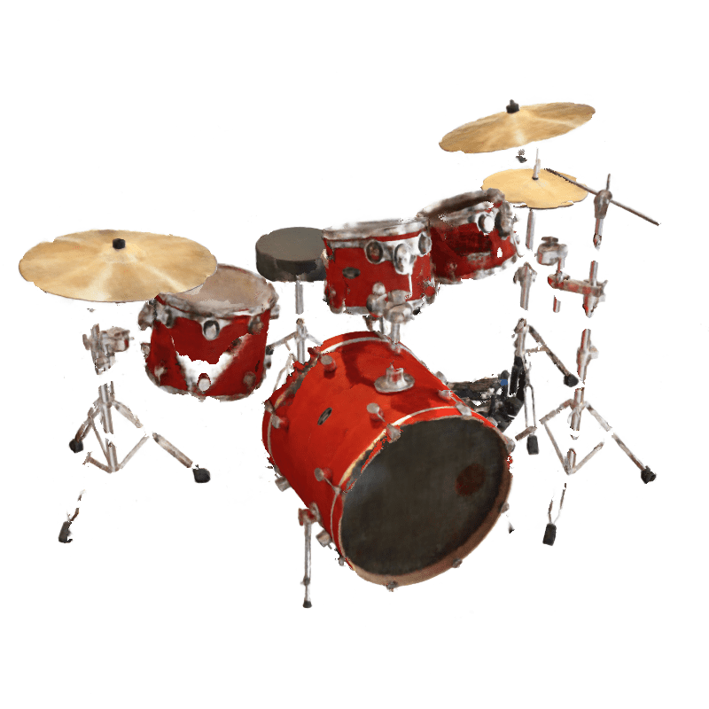
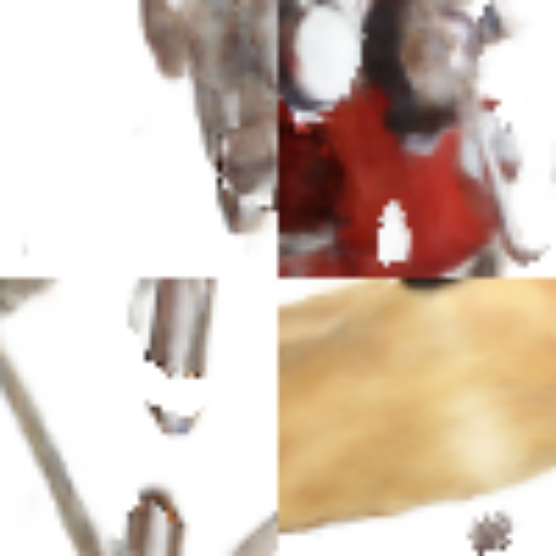
(b) NeRF[22]

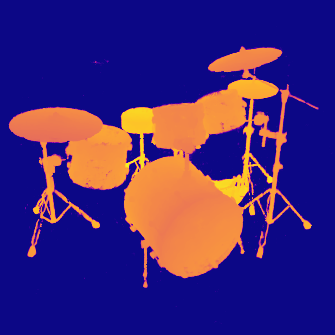
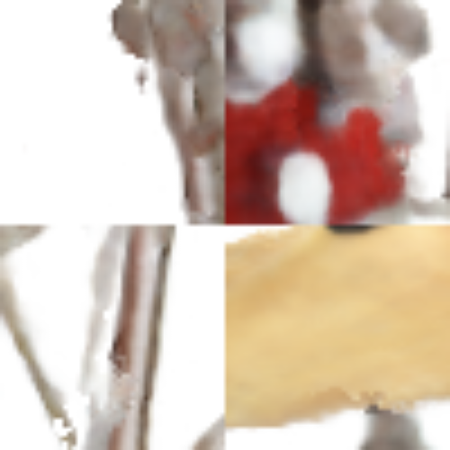
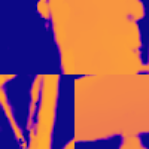
(c) KiloNeRF[26]

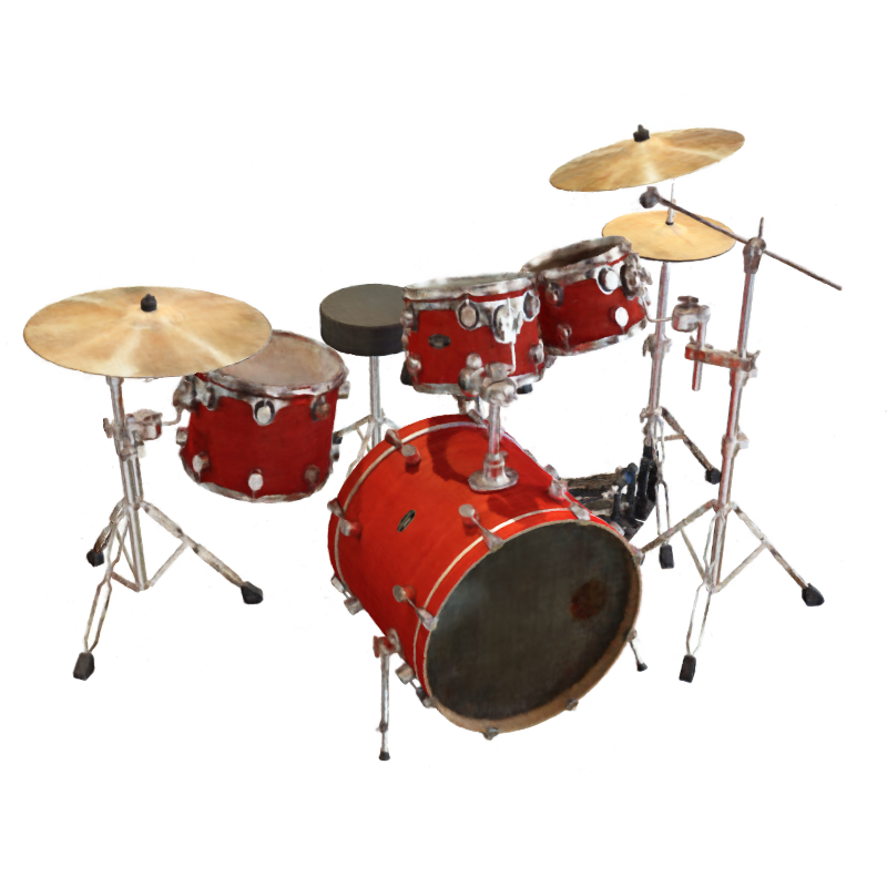
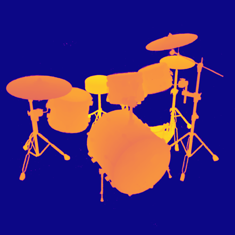
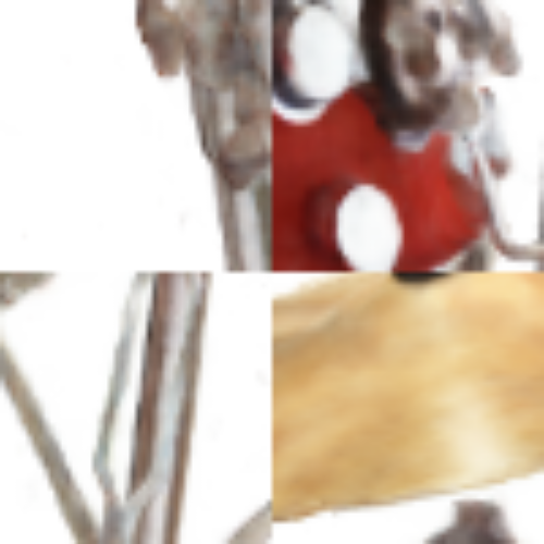
(d) Our

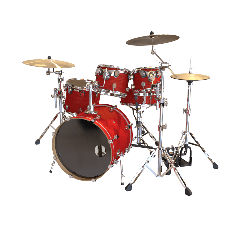
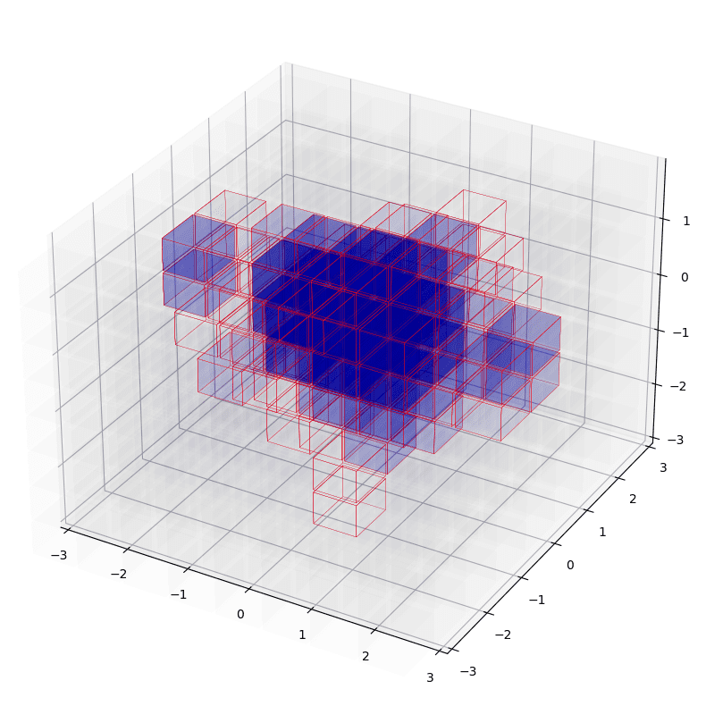
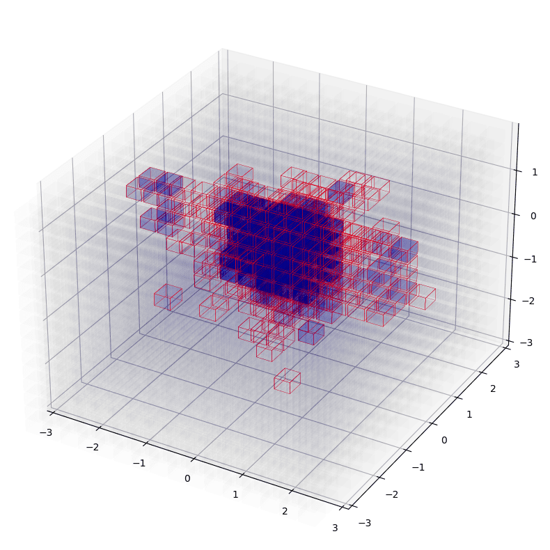
(e) Octree

Figure 10: Visual Comparison on synthetic NeRF dataset [22]. (a) is ground truth view with zoom in details. (b), (c), (d) are state-of-the-arts methods of NeRF [22], KiloNeRF [26], and our proposed method with highlighted detail regions. (e) illustrate example view and octree optimization process from coarse to fine (Blocks with green line indicates block merging, and red line indicates blocks splitting).

Fig. (10) shows visual comparisons on the synthetic NeRF dataset. All the state-of-the-art methods achieve reasonable performance in rendering novel views from camera positions close to the training views. However, in visualizations of the depth map scene, NeRF [22] shows blurring and topological artifacts in the depth, indicating that the actual 3D structure is less accurate. As we show below, this has an impact on the quality of extrapolated views far from the training data. KiloNeRF [26] shows high quality results in the RGB view, but exhibits a slight blocking effect when visualizing the depth view, since KiloNeRF’s sub-network are pre-trained by a global network, i.e., NeRF, each sub-network is independent in the pre-training stage and mix the query results in the fine-tuning stage, which introduces a discontinuity. Our method takes advantage of the tree structure for flexible and scalable representation with an adaptive training scheme for computational resource allocation, all the sub-networks are trained from coarse to fine. Therefore, no pre-training is required, and back propagation will update all sub-network along the integral ray direction, which shows consistent and smooth rendering results in both RGB view and depth. To better illustrate our octree-based representation, we also show a progression of the octree update last column (ground truth rendering on top).

8.1 Extreme Novel View Comparison

In this section, we show the extensive comparison in details for extreme view of real scene dataset. Fig. (11) shows the novel view synthesis with view rotation radius $R=1.5$, our method shows similar performance with MipNeRF [3], but outperforms NeRF and KiloNeRF in details texture recovering. Fig. (12) increase rotation radius for extreme view rendering, NeRF, KiloNeRF and MipNeRF show significant false trails in extrapolated view due to neural network tends to output unknown density value in extrapolated part of scene. Octtree could explicitly define rendering space, and significantly allevate rendering trails. Alought KiloNeRF can also use pre-trained octtree to accelerate rendering process, it still require train a extra single network for model distilling, thus reserve same trails effect in the fine-tune stage. Fig. (13) also shows more comparison for extrapolated novel view synthesis, our method outperform other alternatives, see details for better visual comparison.

(a) NeRF[22]

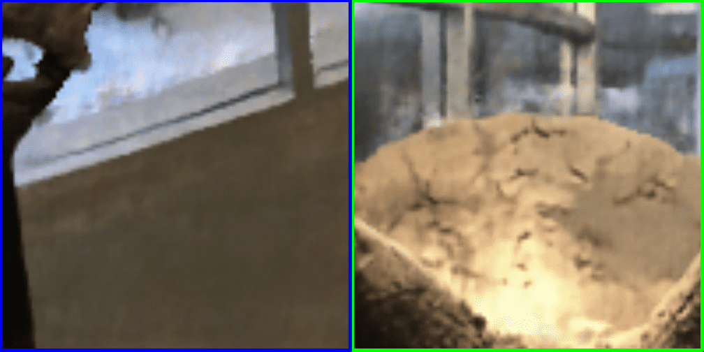
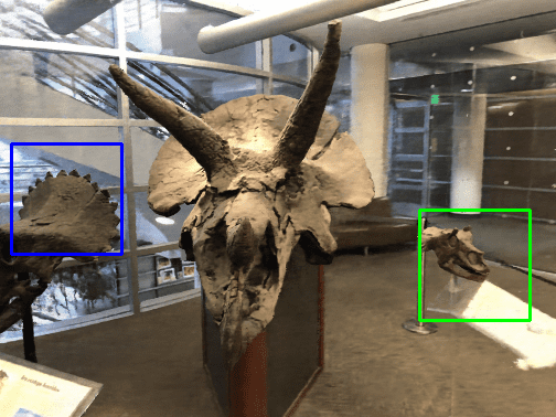
(b) KiloNeRF

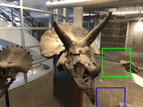
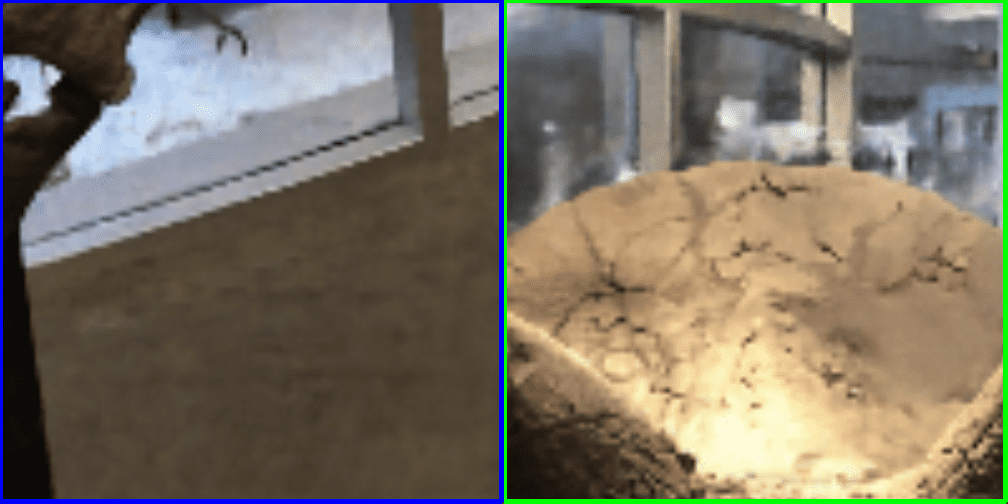
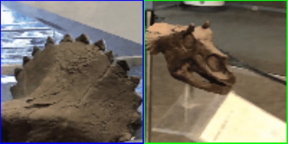
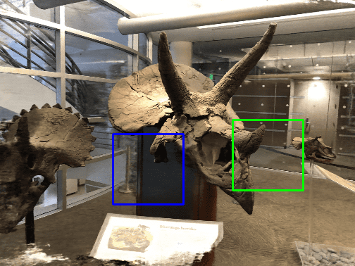
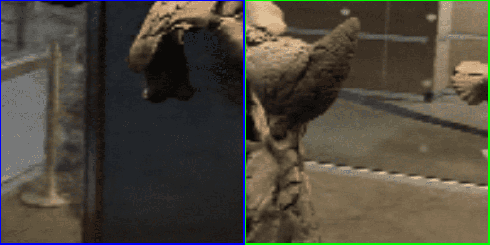
(c) MipNeRF

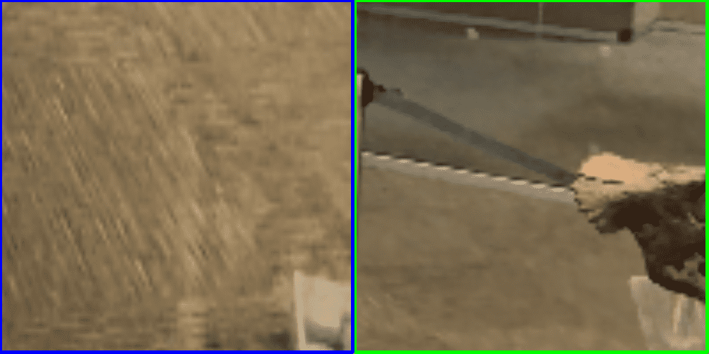
(d) Our

Figure 11: Extreme novel view synthesis for HORNS dataset with view rotation $R=1.5$. We compare our method against NeRF [22], KiloNeRF [26], MipNeRF [3].

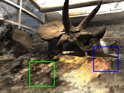
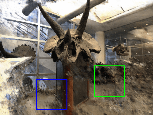
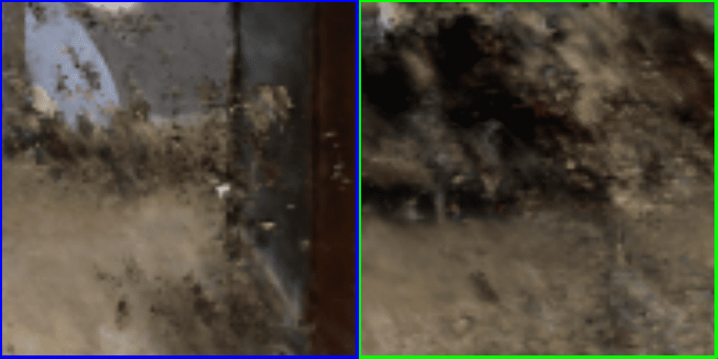
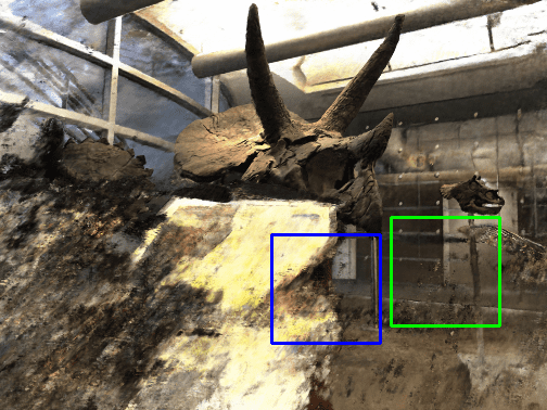
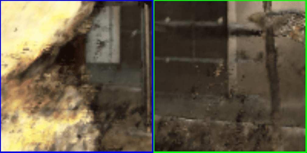
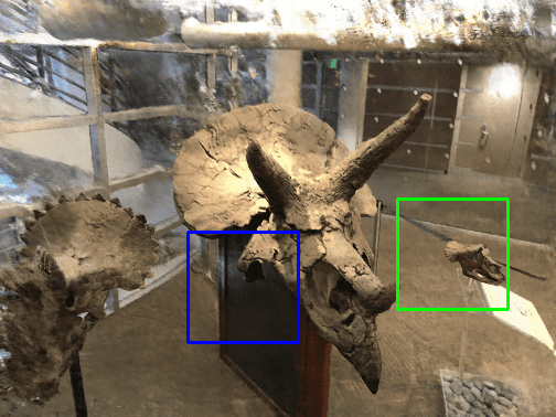
(a) NeRF[22]

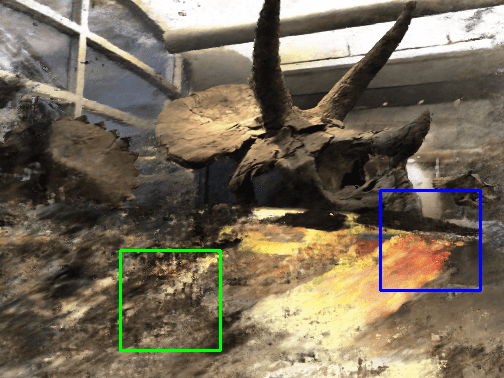
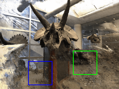
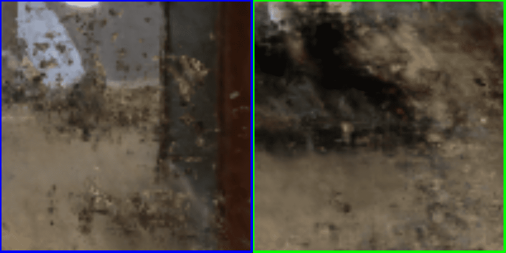
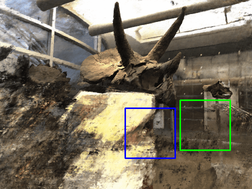
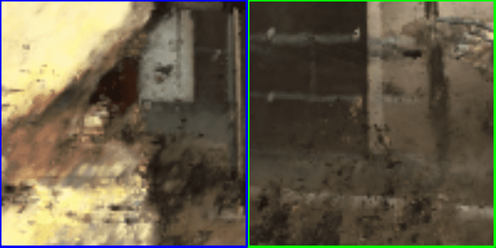
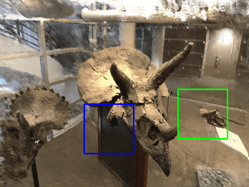
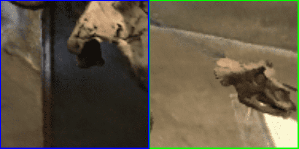
(b) KiloNeRF[26]

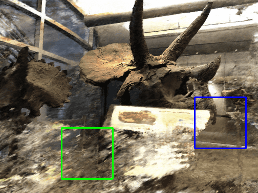
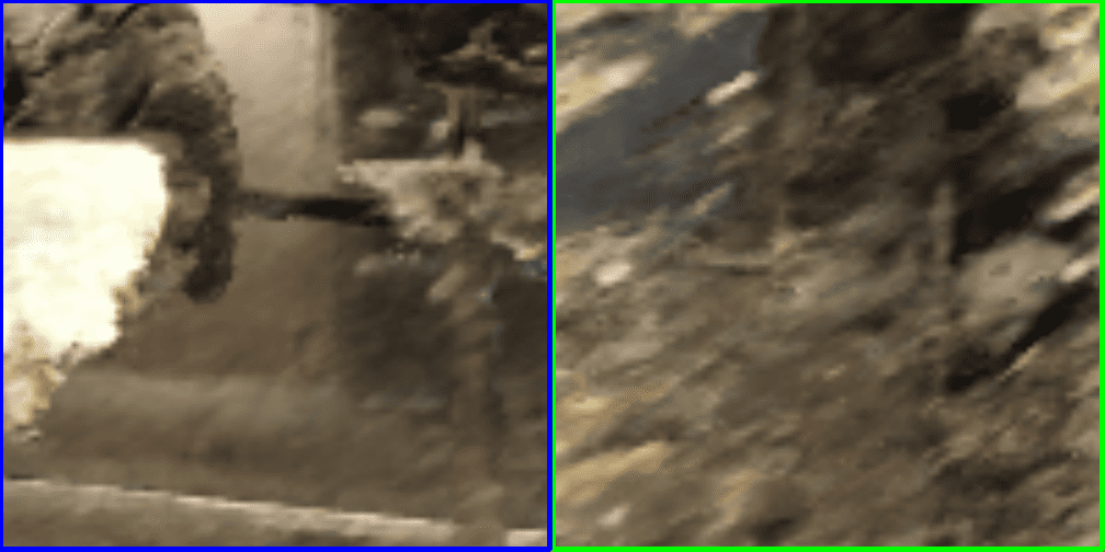
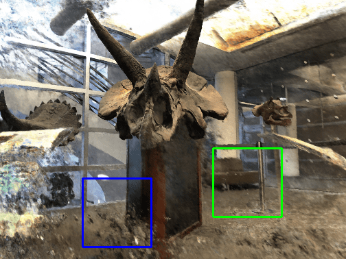
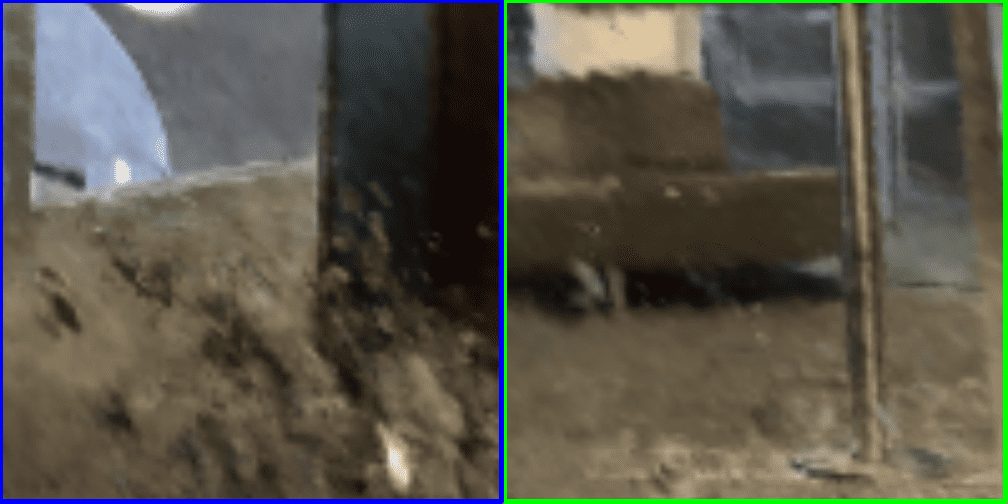
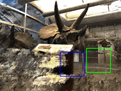
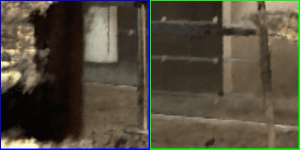
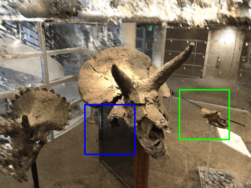
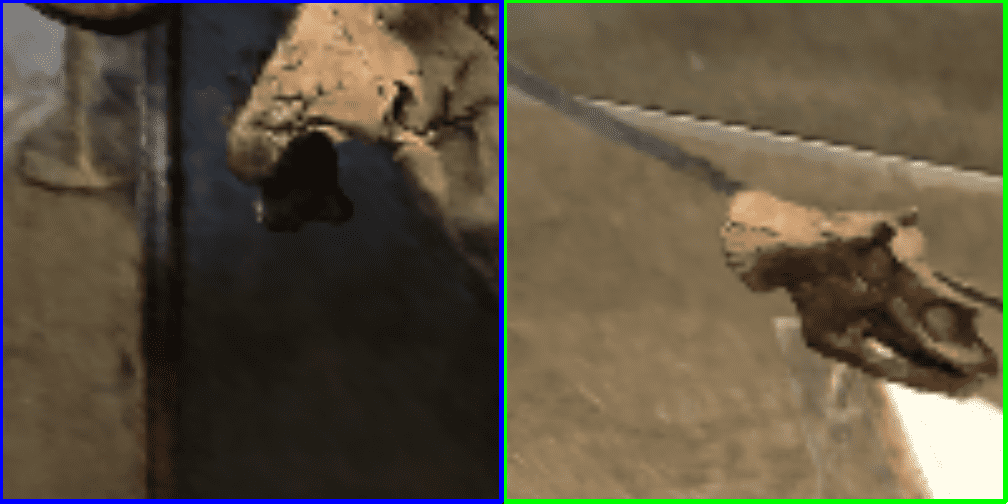
(c) MipNeRF[3]

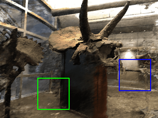
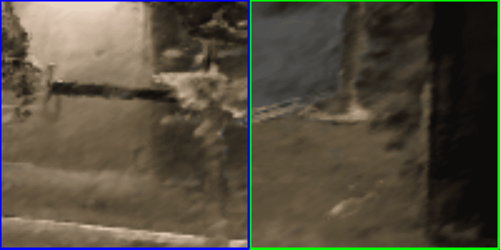
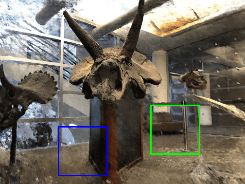
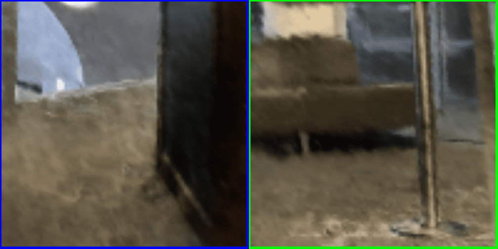
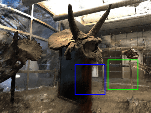
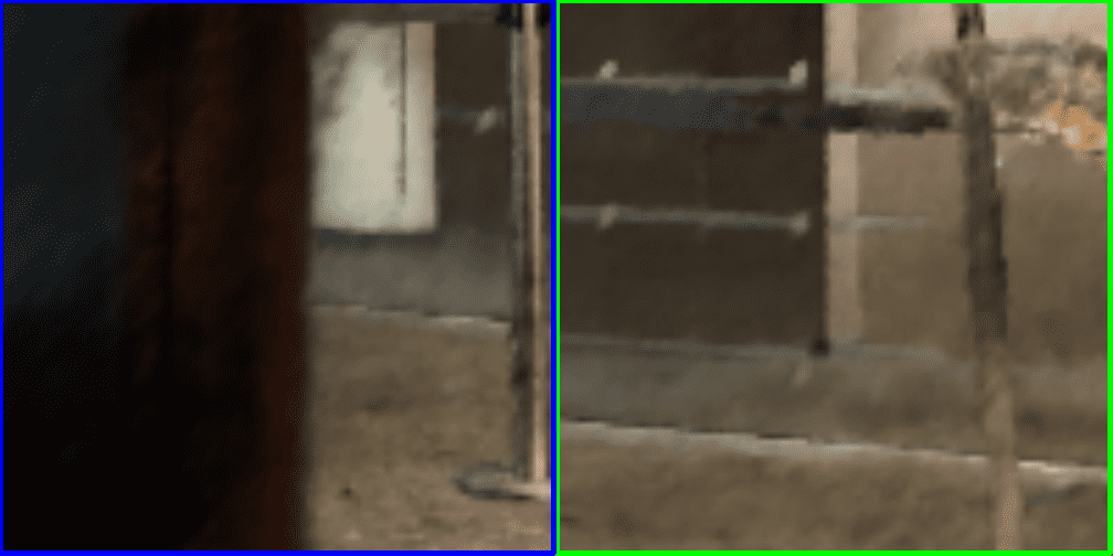
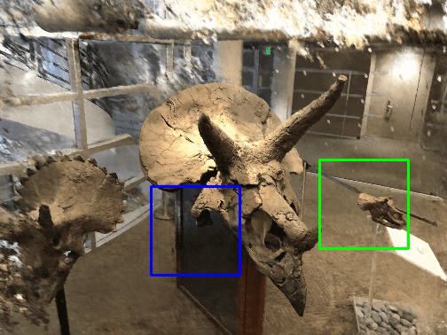
(d) Our

Figure 12: Extreme novel view synthesis for HORNS dataset with view rotation $R=3.0$. We compare our method against NeRF [22], KiloNeRF [26], MipNeRF [3].

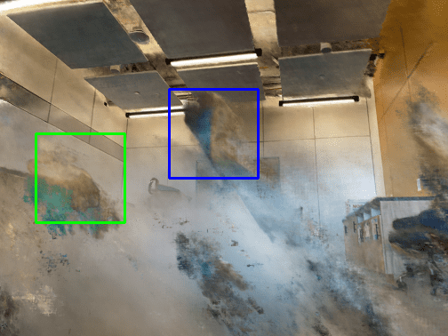
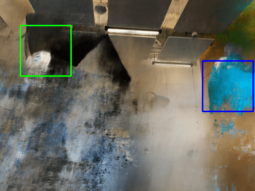
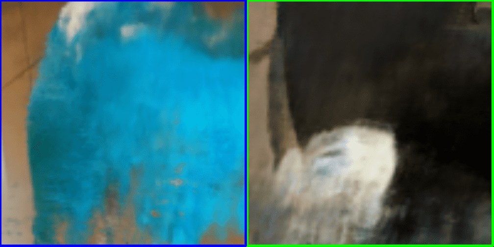
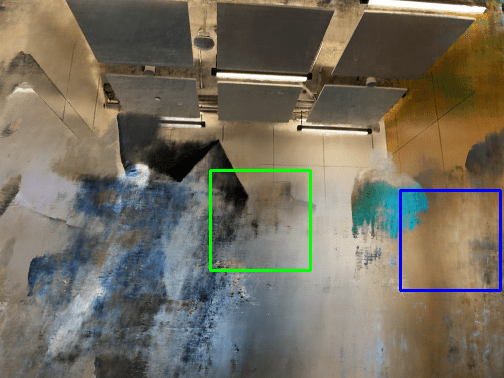
(a) NeRF[22]

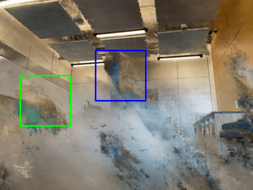
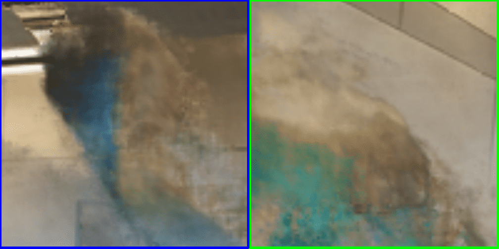
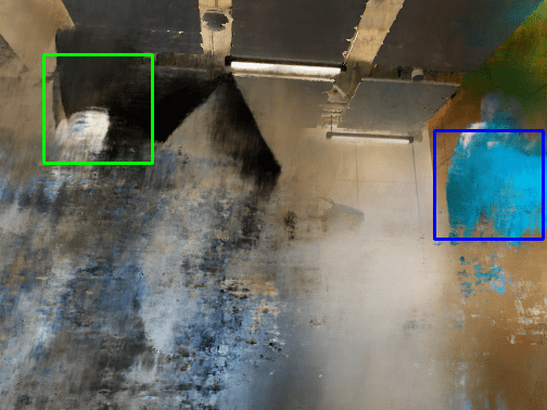
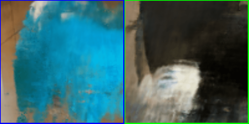
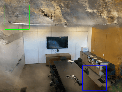
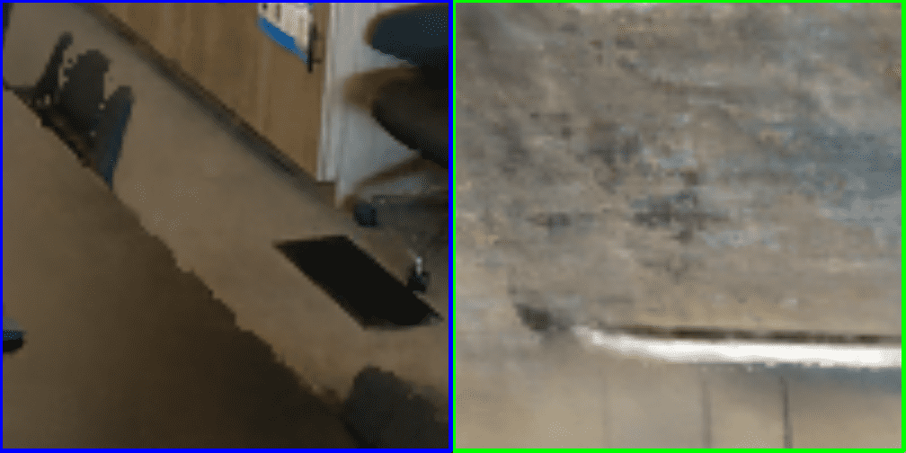
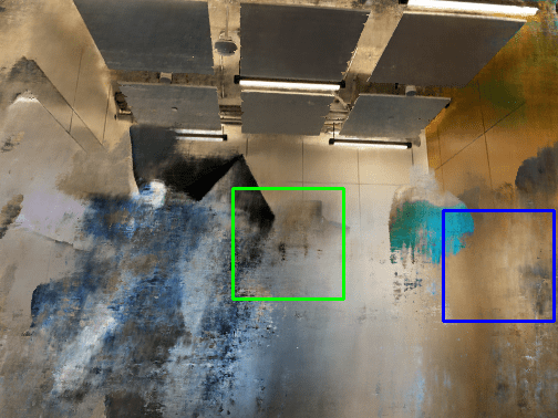
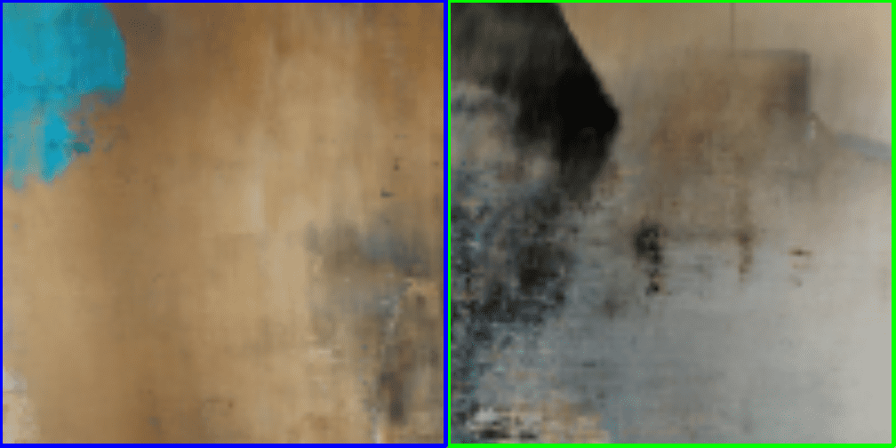
(b) KiloNeRF[26]

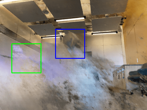
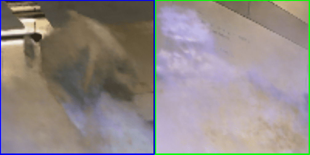
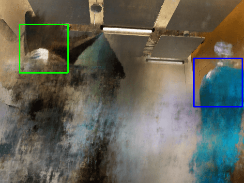
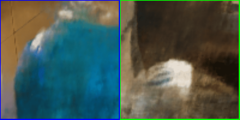
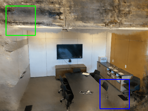
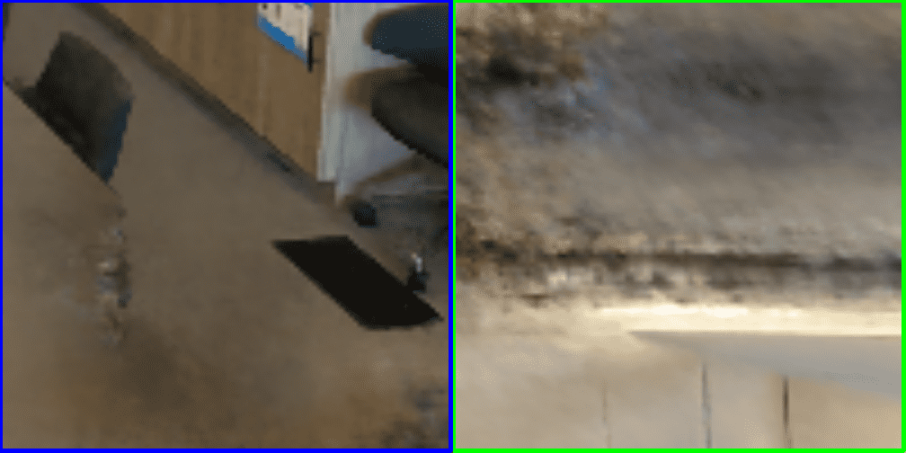
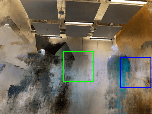
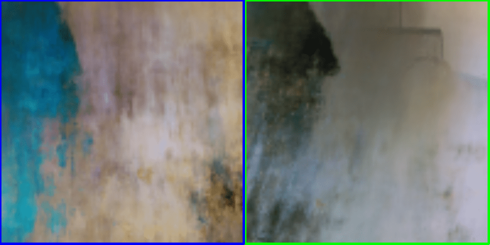
(c) MipNeRF[3]

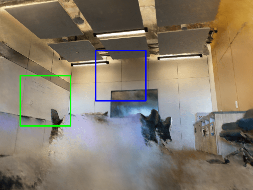
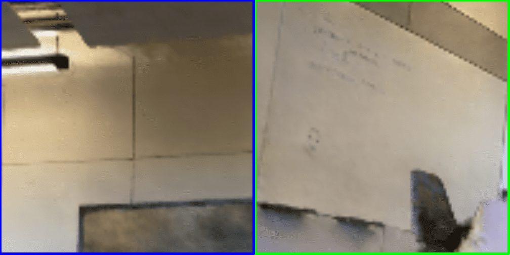
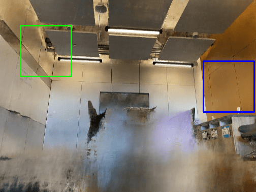
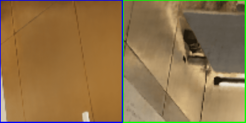
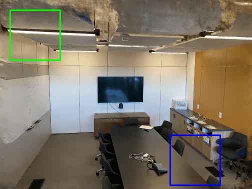
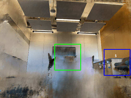
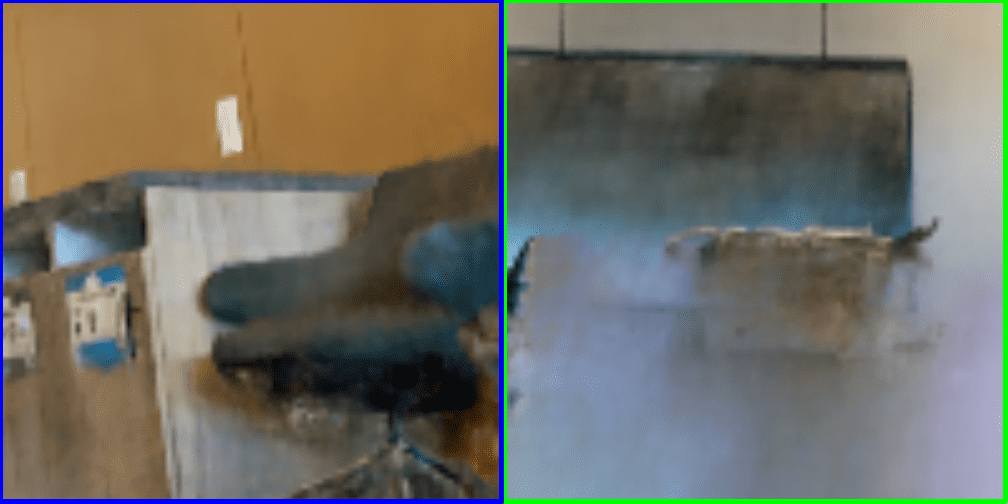
(d) Our

Figure 13: Extreme novel view synthesis for ROOMS dataset with view rotation $R=3.0$. We compare our method against NeRF [22], KiloNeRF [26], MipNeRF [3].

8.2 UAV Scene Reconstruction

In this section, we show the results of ground scene reconstruction from UAV video in Fig. (14). UAV views contain comparatively large viewpoint and camera pose change, which is a challengine task for neural rendering. NeRF [22] shows blur rendering results due to incorrect density estimation of scene. MipNeRF [3] fails to estimate correct density in second row of results, partially because a large viewpoint changes leads to sample in the space that has insufficient training samples and outputs random density values. Our method takes advantage of (1) octtree that bounds whole scene and skip empty space, and (2) distributed sub-network architecture that trains and renders locally to avoid inbalanced sampling inside each octtree nodes and adaptively reallocate computational resource for each node.

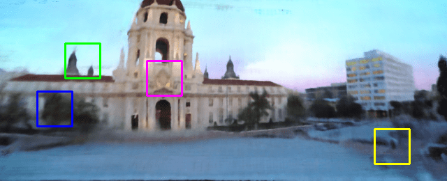
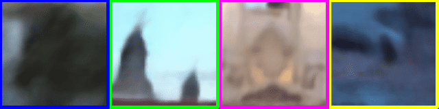
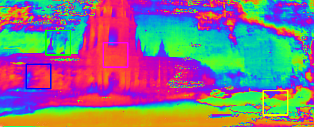
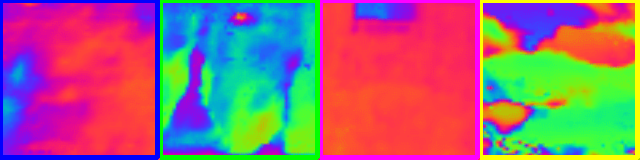
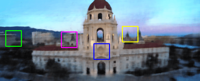
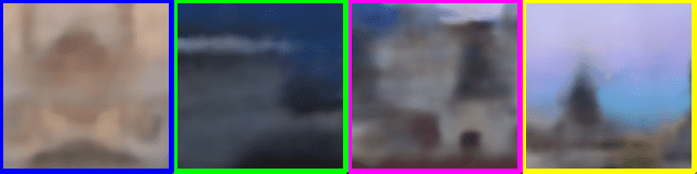
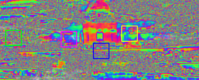
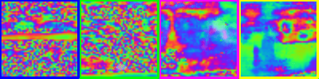
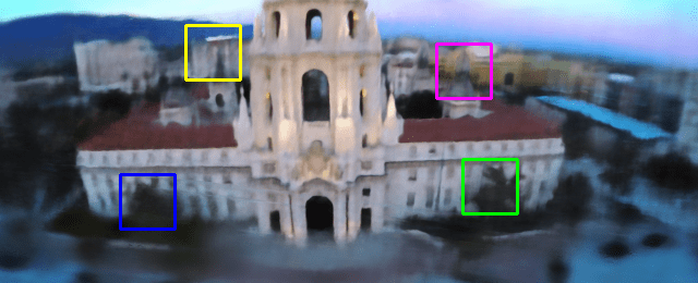
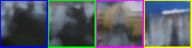
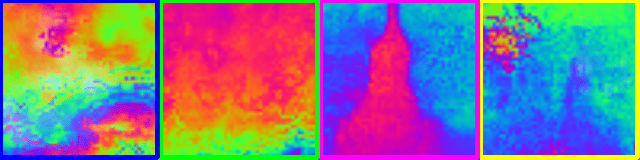
(a) NeRF[22]

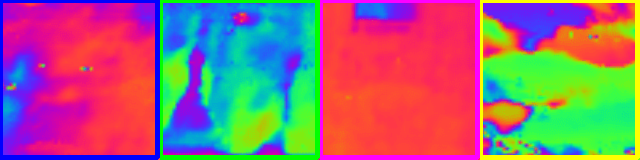
v

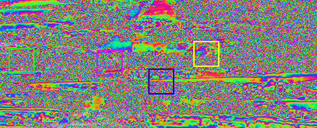
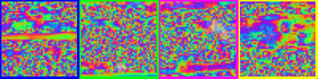
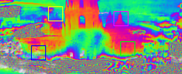
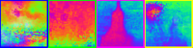
(b) MipNeRF[3]

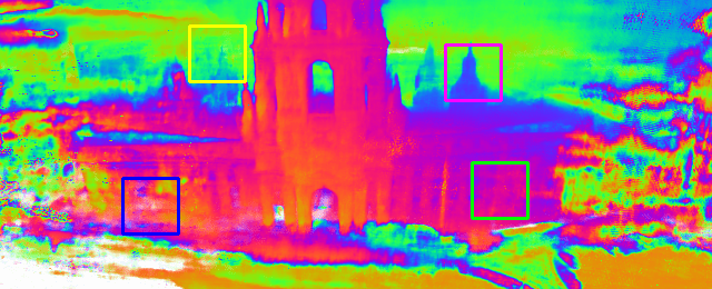
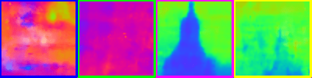
(c) Our

Figure 14: UAV scene reconstruction. We compare our method against NeRF [22], KiloNeRF [26], MipNeRF [3].

References

- [1] Aharchi, M., Kbir, M.A.: A review on 3D reconstruction techniques from 2D images. In: The Proceedings of the Third International Conference on Smart City Applications. pp. 510–522. Springer (2019)
- [2] Aliev, K.A., Sevastopolsky, A., Kolos, M., Ulyanov, D., Lempitsky, V.: Neural point-based graphics. In: Computer Vision–ECCV 2020: 16th European Conference, Glasgow, UK, August 23–28, 2020, Proceedings, Part XXII 16. pp. 696–712. Springer (2020)
- [3] Barron, J.T., Mildenhall, B., Tancik, M., Hedman, P., Martin-Brualla, R., Srinivasan, P.P.: Mip-nerf: A multiscale representation for anti-aliasing neural radiance fields. In: ICCV (2021)
- [4] Boss, M., Braun, R., Jampani, V., Barron, J.T., Liu, C., Lensch, H.: Nerd: Neural reflectance decomposition from image collections. In: Proceedings of the IEEE/CVF International Conference on Computer Vision. pp. 12684–12694 (2021)
- [5] Chan, E.R., Monteiro, M., Kellnhofer, P., Wu, J., Wetzstein, G.: pi-gan: Periodic implicit generative adversarial networks for 3d-aware image synthesis. In: Proceedings of the IEEE/CVF Conference on Computer Vision and Pattern Recognition. pp. 5799–5809 (2021)
- [6] Chibane, J., Pons-Moll, G.: Implicit feature networks for texture completion from partial 3d data. In: European Conference on Computer Vision. pp. 717–725. Springer (2020)
- [7] Dahnert, M., Hou, J., Nießner, M., Dai, A.: Panoptic 3d scene reconstruction from a single rgb image. Advances in Neural Information Processing Systems 34 (2021)
- [8] Eslami, S.A., Rezende, D.J., Besse, F., Viola, F., Morcos, A.S., Garnelo, M., Ruderman, A., Rusu, A.A., Danihelka, I., Gregor, K., et al.: Neural scene representation and rendering. Science 360(6394), 1204–1210 (2018)
- [9] Flynn, J., Broxton, M., Debevec, P., DuVall, M., Fyffe, G., Overbeck, R., Snavely, N., Tucker, R.: Deepview: View synthesis with learned gradient descent. In: Proceedings of the IEEE/CVF Conference on Computer Vision and Pattern Recognition. pp. 2367–2376 (2019)
- [10] Garbin, S.J., Kowalski, M., Johnson, M., Shotton, J., Valentin, J.: FastNeRF: High-fidelity neural rendering at 200fps. arXiv preprint arXiv:2103.10380 (2021)
- [11] Gurram, P., Lach, S., Saber, E., Rhody, H., Kerekes, J.: 3d scene reconstruction through a fusion of passive video and lidar imagery. In: 36th Applied Imagery Pattern Recognition Workshop (aipr 2007). pp. 133–138. IEEE (2007)
- [12] Ham, H., Wesley, J., Hendra, H.: Computer vision based 3D reconstruction: A review. International Journal of Electrical and Computer Engineering 9(4), 2394 (2019)
- [13] Hedman, P., Philip, J., Price, T., Frahm, J.M., Drettakis, G., Brostow, G.: Deep blending for free-viewpoint image-based rendering. ACM Transactions on Graphics (TOG) 37(6), 1–15 (2018)
- [14] Jensen, R., Dahl, A., Vogiatzis, G., Tola, E., Aanæs, H.: Large scale multi-view stereopsis evaluation. In: 2014 IEEE Conference on Computer Vision and Pattern Recognition. pp. 406–413. IEEE (2014)
- [15] Kühner, T., Kümmerle, J.: Large-scale volumetric scene reconstruction using lidar. In: 2020 IEEE International Conference on Robotics and Automation (ICRA). pp. 6261–6267. IEEE (2020)
- [16] Lin, C.H., Ma, W.C., Torralba, A., Lucey, S.: BARF: Bundle-adjusting neural radiance fields. In: Proceedings of the IEEE/CVF International Conference on Computer Vision (ICCV). pp. 5741–5751 (October 2021)
- [17] Lindell, D.B., Martel, J.N., Wetzstein, G.: AutoInt: Automatic integration for fast neural volume rendering. In: CVPR (2021)
- [18] Liu, L., Gu, J., Lin, K.Z., Chua, T.S., Theobalt, C.: Neural sparse voxel fields. NeurIPS (2020)
- [19] Martel, J.N., Lindell, D.B., Lin, C.Z., Chan, E.R., Monteiro, M., Wetzstein, G.: ACORN: Adaptive coordinate networks for neural representation. ACM Trans. Graph. (SIGGRAPH) (2021)
- [20] Meshry, M., Goldman, D.B., Khamis, S., Hoppe, H., Pandey, R., Snavely, N., Martin-Brualla, R.: Neural rerendering in the wild. In: CVPR. pp. 6878–6887 (2019)
- [21] Mildenhall, B., Srinivasan, P.P., Ortiz-Cayon, R., Kalantari, N.K., Ramamoorthi, R., Ng, R., Kar, A.: Local light field fusion: Practical view synthesis with prescriptive sampling guidelines. ACM Transactions on Graphics (TOG) (2019)
- [22] Mildenhall, B., Srinivasan, P.P., Tancik, M., Barron, J.T., Ramamoorthi, R., Ng, R.: Nerf: Representing scenes as neural radiance fields for view synthesis. In: ECCV (2020)
- [23] Niemeyer, M., Mescheder, L., Oechsle, M., Geiger, A.: Differentiable volumetric rendering: Learning implicit 3d representations without 3d supervision. In: Proceedings of the IEEE/CVF Conference on Computer Vision and Pattern Recognition. pp. 3504–3515 (2020)
- [24] Oechsle, M., Mescheder, L., Niemeyer, M., Strauss, T., Geiger, A.: Texture fields: Learning texture representations in function space. In: Proceedings of the IEEE/CVF International Conference on Computer Vision. pp. 4531–4540 (2019)
- [25] Park, J.J., Florence, P., Straub, J., Newcombe, R., Lovegrove, S.: Deepsdf: Learning continuous signed distance functions for shape representation. In: Proceedings of the IEEE/CVF Conference on Computer Vision and Pattern Recognition. pp. 165–174 (2019)
- [26] Reiser, C., Peng, S., Liao, Y., Geiger, A.: KiloNeRF: Speeding up neural radiance fields with thousands of tiny mlps. In: International Conference on Computer Vision (ICCV) (2021)
- [27] Saito, S., Huang, Z., Natsume, R., Morishima, S., Kanazawa, A., Li, H.: Pifu: Pixel-aligned implicit function for high-resolution clothed human digitization. In: Proceedings of the IEEE/CVF International Conference on Computer Vision. pp. 2304–2314 (2019)
- [28] Schonberger, J.L., Frahm, J.M.: Structure-from-motion revisited. In: Proceedings of the IEEE conference on computer vision and pattern recognition. pp. 4104–4113 (2016)
- [29] Schwarz, K., Liao, Y., Niemeyer, M., Geiger, A.: Graf: Generative radiance fields for 3d-aware image synthesis. arXiv preprint arXiv:2007.02442 (2020)
- [30] Seitz, S.M., Curless, B., Diebel, J., Scharstein, D., Szeliski, R.: A comparison and evaluation of multi-view stereo reconstruction algorithms. In: 2006 IEEE computer society conference on computer vision and pattern recognition (CVPR’06). vol. 1, pp. 519–528. IEEE (2006)
- [31] Sitzmann, V., Martel, J.N., Bergman, A.W., Lindell, D.B., Wetzstein, G.: Implicit neural representations with periodic activation functions. In: Proc. NeurIPS (2020)
- [32] Sitzmann, V., Thies, J., Heide, F., Nießner, M., Wetzstein, G., Zollhofer, M.: Deepvoxels: Learning persistent 3d feature embeddings. In: Proceedings of the IEEE/CVF Conference on Computer Vision and Pattern Recognition. pp. 2437–2446 (2019)
- [33] Sitzmann, V., Zollhöfer, M., Wetzstein, G.: Scene representation networks: Continuous 3d-structure-aware neural s cene representations. arXiv preprint arXiv:1906.01618 (2019)
- [34] Srinivasan, P.P., Deng, B., Zhang, X., Tancik, M., Mildenhall, B., Barron, J.T.: NeRV: Neural reflectance and visibility fields for relighting and view synthesis. In: Proceedings of the IEEE/CVF Conference on Computer Vision and Pattern Recognition. pp. 7495–7504 (2021)
- [35] Tewari, A., Fried, O., Thies, J., Sitzmann, V., Lombardi, S., Sunkavalli, K., Martin-Brualla, R., Simon, T., Saragih, J., Nießner, M., et al.: State of the art on neural rendering. In: Computer Graphics Forum. vol. 39, pp. 701–727. Wiley Online Library (2020)
- [36] Xian, W., Huang, J.B., Kopf, J., Kim, C.: Space-time neural irradiance fields for free-viewpoint video. In: Proceedings of the IEEE/CVF Conference on Computer Vision and Pattern Recognition. pp. 9421–9431 (2021)
- [37] Xiang, F., Xu, Z., Hasan, M., Hold-Geoffroy, Y., Sunkavalli, K., Su, H.: NeuTex: Neural texture mapping for volumetric neural rendering. In: Proceedings of the IEEE/CVF Conference on Computer Vision and Pattern Recognition. pp. 7119–7128 (2021)
- [38] Yifan, W., Wu, S., Öztireli, C., Sorkine-Hornung, O.: Iso-points: Optimizing neural implicit surfaces with hybrid representations. In: CVPR (2021)
- [39] Yu, A., Li, R., Tancik, M., Li, H., Ng, R., Kanazawa, A.: PlenOctrees for real-time rendering of neural radiance fields. In: ICCV (2021)
- [40] Yu, A., Ye, V., Tancik, M., Kanazawa, A.: pixelNeRF: Neural radiance fields from one or few images. In: CVPR (2021)
- [41] Zhang, K., Luan, F., Wang, Q., Bala, K., Snavely, N.: PhySG: Inverse rendering with spherical gaussians for physics-based material editing and relighting. In: Proceedings of the IEEE/CVF Conference on Computer Vision and Pattern Recognition. pp. 5453–5462 (2021)
- [42] Zhang, R., Isola, P., Efros, A.A., Shechtman, E., Wang, O.: The unreasonable effectiveness of deep features as a perceptual metric. In: CVPR (2018)
- [43] Zhou, T., Tucker, R., Flynn, J., Fyffe, G., Snavely, N.: Stereo magnification: Learning view synthesis using multiplane images. arXiv preprint arXiv:1805.09817 (2018)
- [44] Zollhöfer, M., Stotko, P., Görlitz, A., Theobalt, C., Nießner, M., Klein, R., Kolb, A.: State of the art on 3D reconstruction with RGB-D cameras. In: Computer graphics forum. vol. 37, pp. 625–652. Wiley Online Library (2018)