MERCURY AND ORBFIT PACKAGES FOR NUMERICAL INTEGRATION OF PLANETARY SYSTEMS: IMPLEMENTATION OF THE YARKOVSKY AND YORP EFFECTS

1 INTRODUCTION

The dynamics of Solar System objects is determined by their mutual gravitational interactions. However, proper modeling of the dynamics of small Solar System objects, smaller than about 30-40 km in size, also requires non-gravitational forces to be included in the model. For asteroids, two relevant such effects are the Yarkovsky and Yarkovsky-O’Keefe-Radzievskii-Paddack (YORP). The Yarkovsky effect is caused by sunlight. When an asteroid heats up in the Sun, it eventually re-radiates the energy away as heat, creating a tiny thrust. This recoil acceleration is much weaker than the gravitational forces, but it can produce substantial orbital changes over long timescales. The same physical phenomenon is also responsible for the YORP effect, a thermal torque that, complemented by a torque produced by scattered sunlight, can modify the rotation rates and obliquities of small bodies as well (see e.g. Bottke et al. 2006, Vokrouhlický et al. 2015). Therefore, the Yarkovsky effect changes the orbital motion of an asteroid, while the YORP effect changes the spin state. However, as the magnitude of the Yarkovsky effect depends on the spin state, the two effects are coupled. For this reason, a high-precision analysis of the orbit evolution of small objects requires both effects to be considered.

It has been proven that the Yarkovsky and YORP effects play an important role in several phenomena in our Solar System, including the transport of objects from the asteroid belt to the near-Earth region (e.g. Farinella and Vokrouhlicky 1999, Bottke et al. 2002, Granvik et al. 2017), the spreading of asteroid families (e.g. Vokrouhlický et al. 2006, Spoto et al. 2015), and evaluation of the impact risks (e.g. Del Vigna et al. 2019, Roa et al. 2021).

Nowadays, numerical integrators are fundamental tools to study problems of celestial mechanics. In the context of our Solar System, long-term numerical simulations are often needed to understand and constrain the past dynamical evolution of planets, satellites, asteroids, and comets. Over the years, different integration schemes have been developed to propagate the gravitational $N$-body problem, and most of them have been included in software packages written in different programming languages. The three most widely used numerical integration packages in the planetary science community are swift (Levison and Duncan 1994), mercury (Chambers and Migliorini 1997), and orbit9 (Milani and Nobili 1988) that is included in the OrbFit package. In addition to these well established packages, rebound (Rein and Liu 2012) became a top-rated tool in the last few years. The last decade also saw a fast improvement in the performances of graphical processing units (GPUs). GPUs can efficiently handle parallel computing, and for this reason, packages such as genga (Grimm and Stadel 2014) have been developed to exploit the advantages of this kind of hardware. Finally, new integrators are also under development (e.g. Zhang and Gladman 2022), answering the need for increased computational and modeling demands.

In the basic version of these integrators, stars and planets are treated as point masses, and their orbits evolve according to their mutual gravitational attraction. On the other hand, small bodies such as asteroids and comets are treated as massless particles, meaning that their dynamics is influenced by the gravitational attraction of stars and planets, but they do not cause any additional force on other bodies. Some of these integrators also include effects due to the oblateness of the central body, or relativistic effects. An example is the mercury-t extension of the mercury code, which takes into account tides, general relativity, and the effect of rotation-induced flattening in order to simulate the dynamical and tidal evolution of multi-planet systems (Bolmont et al. 2015).

Among the public distributions of $N$-body codes mentioned above, the Yarkovsky effect has been implemented in swift, genga and orbit9, while only swift has also the YORP effect implemented (Brož et al. 2011). This modified version of swift has been made available to the community. On the other hand, several different effects have been added in the rebound integrator (Tamayo et al. 2020), but the Yarkovsky and YORP effects are still not among those.

In this paper, we describe our implementation of the Yarkovsky/YORP effect in the mercury and orbit9 integrators. Both integrators have been extensively used for the simulations of the long-term orbit evolution of asteroids. For recent examples of mercury based simulations see e.g. Hsieh et al. (2020), -Došović et al. (2020), Martin and Livio (2021), while for recent works based on orbit9 see e.g. Knežević (2020), Pavela et al. (2021), Dermott et al. (2021). Despite being extensively used, the Yarkovsky and YORP effects are not included in the mercury package. The orbit9 integrator does not include the YORP effect, while the Yarkovsky was implemented using a very simplified formulation (see e.g. Novaković et al. 2015).

To implement the two effects in the mercury and orbit9 integrators we adopted the following strategy. The Yarkovsky effect is computed as a non-conservative vector field along the tangential direction, that produces the semi-major axis drift given by analytical theories (see, e.g. Vokrouhlický 1999). For the YORP effect, we follow a similar approach to the one described in Bottke et al. (2015), which is suitable for statistical studies of the evolution of asteroids. In our code, we provide two different YORP models: a static and a stochastic one. Along with the two effects, we introduced the effect of collisions and breakups on the asteroid spin state.

Finally, in addition to the details on the implementation, we performed tests to validate the new codes. In this respect, we first show that the integrations obtained with the two packages agree with each other. We also provide some additional tests to show how the static and stochastic YORP model works.

The extended version of the mercury integrator is publicly available at https://github.com/Fenu24/mercury, while the modified version of orbit9 can be found at https://github.com/Fenu24/OrbFit.

2 THE mercury AND orbit9 INTEGRATORS

In this section we provide more details about mercury and orbit9 $N$-body software packages.

2.1 The mercury package

The mercury integrator package is written in fortran language, and it contains several integration schemes: a general Bulirsch-Stoer algorithm (see e.g. Bulirsch and Stoer 2002), a Radau integrator (Everhart 1985), a second order mixed-variable symplectic (MVS) integrator (Wisdom et al. 1996), and a hybrid symplectic integrator (Chambers 1999) that is able to handle close encounters with planets.

mercury is designed to compute the evolution of objects moving around a massive central body, such as planets and asteroids around the Sun, a system of moons around a planet, or exo-planetary systems. The integrators include the gravitational forces due to the central mass, and some other specified massive bodies. It can also compute non-gravitational forces for comets (Marsden et al. 1973), or compute the effects of the gravitational $J_{2},J_{4},J_{6}$ moments of the central body.

Other forces depending on the positions and velocities can be added by editing the subroutine mfo_user. The Yarkovsky effect is directly implemented here as described in Sec. 3. The integration of the spin-axis dynamics is performed in the main integration loop of the orbital dynamics. The spin-axis and the rotation rate evolve on a time scale much larger than the orbital period, hence a longer time-step is used. At each integration step of the orbital dynamics, we check whether an integration step for the spin-axis dynamics is needed or not. In the positive case, the obliquity and the rotation rate are updated as described in Sec. 4, and the semi-major axis drift due to the Yarkovsky effect is recomputed. The subroutines used for these tasks are all implemented in an external module named yorp_module.

On a more technical side, mercury is capable to detect collisions between a planet (or the central body) and a massless object, or to detect an escape from the system. When either of these occur, the array containing the IDs of objects is re-sized and re-arranged in order to remove the colliding (or escaping) particle from the integration. The indexing of the objects is therefore changed at every removal event. The arrays containing all the parameters needed for the coupled Yarkovsky/YORP effect dynamics are re-arranged as well, according to the new objects’ indexing.

2.2 The orbit9 integrator from the orbfit package

The orbit9 integrator is included in the orbfit package, and it is also written in fortran language. It includes three different integration schemes: a Radau integrator (Everhart 1985), a symplectic Runge-Kutta-Gauss with variable orders (see e.g. Hairer and Wanner 1996), and a multistep method with symplectic starter (Milani and Nobili 1988).

This package is explicitly designed for the long-term integration of main belt asteroids, and it includes the gravitational attraction of the planets. In the case only the giant gas planets are included in the model, a barycentric correction can be applied to take into account the effects of the missing inner planets. The integrator permits to add to the dynamical model also the quadrupole $J_{2}$ moment of the Sun, and relativistic effects. Details of the implementation can be found in Nobili et al. (1989). This package also includes several useful tools, such as an on-line removal of short periodic effects (Carpino et al. 1987), close approaches monitoring, and the computation of the maximum Lyapounov Characteristics Exponents. Due to all these options, orbit9 is widely used for the computation of proper elements of main-belt asteroids (Knežević and Milani 2000).

Additional forces can be easily added in the subroutine force9. orbit9 already provides a simple implementation of the Yarkovsky effect, in which the semi-major axis drift is provided in input for each asteroid, and then kept constant over the whole integration time-span. For the purpose of this work, we replaced this part with our implementation described in Sec. 3. To include the YORP effect, we used a similar solution to the one described for mercury, and the subroutines for this purpose are all contained in a module called yorp_module.

3 YARKOVSKY EFFECT IMPLEMENTATION

The Yarkovsky effect mainly causes a change in semi-major axis, and the drift $\textrm{d}a/\textrm{d}t$ depends on several orbital and physical parameters of the asteroid, i.e.

$$\frac{\textrm{d}a}{\textrm{d}t}=\bigg{(}\frac{\textrm{d}a}{\textrm{d}t}\bigg{)}(a,D,\rho,K,C,\gamma,P,\alpha,\varepsilon).$$ (1)

In Eq. (1), $a$ is the semi-major axis of the orbit, $D$ is the diameter of the asteroid, $\rho$ is the density, $K$ is the thermal conductivity, $C$ is the heat capacity, $\gamma$ is the obliquity, $P$ is the rotation period, $\alpha$ is the absorption coefficient, and $\varepsilon$ is the emissivity. The total semi-major axis drift is given by the sum of the diurnal and the seasonal effects, i.e.

$$\frac{\textrm{d}a}{\textrm{d}t}=\kappa_{1}\cos\gamma+\kappa_{2}\sin^{2}\gamma,$$ (2)

where $\kappa_{1}$ and $\kappa_{2}$ are functions of the asteroid orbit, physical parameters, and rotation period (see e.g. Vokrouhlický 1998, 1999, Fenucci et al. 2021, Appendix A, for details). The acceleration due to the gravitational attraction of the planets is then augmented with a force of the form $F=F_{\tau}\tau$, where $\tau$ is the tangential direction. The multiplying factor $F_{\tau}$ is obtained through the Gauss planetary equations (see e.g. Murray and Dermott 2000) as

$$F_{\tau}=\frac{\textrm{d}a}{\textrm{d}t}\frac{\sqrt{GM_{\odot}(1-e^{2})}}{2a^{3/2}(1+e\cos f)},$$ (3)

where $G$ is the universal gravitational constant, $M_{\odot}$ is the mass of the Sun, $e$ is the orbital eccentricity, and $f$ is the true anomaly.

The Gauss equation for $\text{d}a/\text{d}t$ also contains the contribution of the radial component $F_{r}$, multiplied by a factor $e\sin f$. The eccentricity of main-belt asteroids is generally small; therefore, we neglected the term containing $F_{r}$ in the derivation of Eq. (3) since its contribution is usually much smaller than that of $F_{\tau}$. Note that the model of the Yarkovsky drift of Eq. (2) is obtained by assuming a circular orbit of the asteroid. While it has been proved that the magnitude of the Yarkovsky effect changes even by an order of magnitude when $e$ passes from $\sim$0.1 to $\sim$0.9 (Spitale and Greenberg 2001), eccentricities up to $\sim$0.3 produce variations only up to $\sim$20% percent with respect to the analytical circular model.

For each small object integrated, the values of $D$, $\rho$, $K$, $C$, $\alpha$, and $\varepsilon$ are provided in input, and they are kept constant throughout the whole integration time-span. We also provide in input the initial values of the obliquity $\gamma$, and of the rotation period $P$, that are used to compute the initial semi-major axis drift, and to set the initial conditions for the spin-axis dynamics.

4 YORP EFFECT IMPLEMENTATION

The strength of the semi-major axis drift of Eq. (2) due to the Yarkovsky effect depends on both the obliquity $\gamma$ and the rotation period $P$. In turn, thermal effects produce a non-zero torque known as YORP effect (see e.g. Bottke et al. 2006), that is able to change both $\gamma$ and $P$. The YORP effect sensitively depends on small surface features, and a precise determination can be done only when a good shape model is known (Vokrouhlický et al. 2015). On the other hand, a Monte Carlo approach can be used to determine the torques for the purpose of statistical studies, as we consider in this work. The evolution of the obliquity $\gamma$ and the rotation rate $\omega=1/P$ are defined by

$$\begin{cases}\displaystyle\frac{\textrm{d}\omega}{\textrm{d}t}&=f(\gamma),\\[8.61108pt] \displaystyle\frac{\textrm{d}\gamma}{\textrm{d}t}&=\displaystyle\frac{g(\gamma)}{\omega},\end{cases}$$ (4)

where $f,g$ are the torques. The selection of these functions is discussed in Sec. 4.1. Eq. (4) is integrated numerically with an explicit Runge-Kutta method of order 4 (see e.g. Bulirsch and Stoer 2002), using a constant time step $\Delta t_{\text{spin}}$. The time step can be either specified by the user or set automatically. The automatic selection is implemented as a simple re-scaling with the minimum diameter $D_{\min}$ among the small bodies, i.e.

$$\Delta t_{\text{spin}}=50\text{ yr}\times\frac{D_{\min}}{1\text{ km}}.$$ (5)

To avoid too short or too long time steps, we set a lower limit of 1 yr and an upper limit of 50 yr. Note that the magnitude of the YORP effect scales as $1/D^{2}$ (see Eq. 6), still the median YORP timescale for objects of $\sim$50 m in diameter is of the order of few thousands years (see e.g. Čapek and Vokrouhlický 2004, Fenucci and Novaković 2021). The re-scaling of Eq. (5) is chosen to slightly reduce the time step for asteroids smaller than 1 km in diameter, while maintaining a good compromise between the accuracy and the speed of the numerical integration.

The YORP effect couples the spin dynamics of the asteroid with the orbital dynamics through the Yarkovsky effect. For this reason, at each integration step of Eq. (4) we also update the value of the semi-major axis drift $\textrm{d}a/\textrm{d}t$ of Eq. (2), by using the new values of $\gamma$ and $P$ obtained from the spin-axis dynamics.

An important issue to deal with when modeling the spin-axis evolution by the YORP effect is handling the asymptotic states. At the asymptotic states, the rotation period becomes either very long or very short, and the currently available YORP effect models are not valid for such extreme cases. The process of an asteroid entering and eventually exiting from an asymptotic state with a new spin state is generally called YORP cycle. We discuss how to handle YORP cycles in Sec. 4.2 and  4.3.

4.1 Choosing the torques

Accurate shape models are known only for a small number of asteroids, and therefore they cannot be used for the purpose a statistical characterization of the YORP torques. Muinonen (1998) introduced the concept of Gaussian random spheres, that are suitable for generating synthetic asteroid shapes. Using this representation, Vokrouhlický and Čapek (2002) computed the thermal torques on a sample of 500 asteroids with mean diameter $D_{0}=2$ km, bulk density $\rho_{0}=2500$ kg m^-3, and placed on a heliocentric circular orbit with radius $a_{0}=2.5$ au, using the approximation of zero thermal conductivity. Later on, Čapek and Vokrouhlický (2004) added the effect of non-zero thermal conductivity in the YORP effect model, and computed the torques for a sample of 200 objects in the cases of conductivity $0.001$ W m^-1 K^-1 and $0.01$ W m^-1 K^-1. Generally, the obliquity $\gamma$ reaches an extreme value of 0, 90, or 180 deg, while the rotation is either accelerated or decelerated.

The statistics for the asymptotic states is sensible to the chosen conductivity. In the case of zero thermal conductivity, Vokrouhlický and Čapek (2002) found that there is approximately the same probability for $\gamma$ to reach 0/180 deg or 90 deg, while the rotation is slowed down asymptotically for the overwhelming majority of the objects. For $K=0.001$ W m^-1 K^-1 Čapek and Vokrouhlický (2004) found that about 80% of the objects are driven towards 0/180 deg in obliquity, while 40% of them asymptotically accelerate the rotation rate. Finally, the authors found that for $K=0.01$ W m^-1 K^-1 about 95% of the objects reach 0/180 deg in obliquity, and there is about the same probability to accelerate or decelerate the rotation rate.

Figure 1 shows the average torques $f,g$ and their variance, computed by Čapek and Vokrouhlický (2004) in the case $K=0.01$ W m^-1 K^-1. Note that $g$ is anti-symmetric with respect to 90 deg, and that it is negative in the interval $(0,90)$ deg. This means that, in this case, the asymptotic values for the obliquity are 0 or 180 deg. On the other hand, $f$ is symmetric with respect to 90 deg and the values at 0 and 180 deg can be either positive or negative, meaning that the objects may accelerate or decelerate asymptotically.

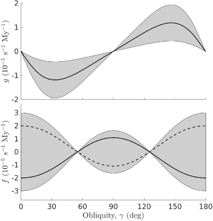
Figure 1: Torques $f,g$ as function of the obliquity $\gamma$ by Čapek and Vokrouhlický (2004), in the case $K=0.01$ W m^-1 K^-1. The black solid curves are the average torques computed over a set of 200 Gaussian random spheres of diameter $D_{0}=2$ km, density $\rho_{0}=2500$ kg m^-3, and placed on circular heliocentric orbits with radius $a_{0}=2.5$ au. The gray zone defines the variance of the results.

In our implementation, the choice of the functions $f,g$ is drawn from the average and variance values shown in Fig. 1, and from the statistics presented in Čapek and Vokrouhlický (2004). Since the computations were not performed on a large enough set of conductivity values, we distinguish two cases: if $K\leq 0.005$ W m^-1 K^-1 we use the distribution of torques obtained for $K=0.001$ W m^-1 K^-1, while we use the distribution obtained for $K=0.01$ W m^-1 K^-1 otherwise.

For the case $K=0.001$ W m^-1 K^-1, we randomly select a function $g$ from the gray area in Fig. 1, and then we decide whether to change its sign or not, according to the 80% probability of reaching 0/180 deg in obliquity. On the other hand, a function $f$ from the gray area is randomly chosen, where the asymptotically accelerating case is selected with 40% probability.

For $K=0.01$ W m^-1 K^-1, we make the simplified assumption that all the objects reach 0/180 deg in obliquity, and that half of the objects accelerate the rotation rate. Hence, here we simply randomly choose a pair $f,g$ from the corresponding gray areas, without any further constraints.

Once $f,g$ are chosen, they also need to be re-scaled to account for different diameter $D$, bulk density $\rho$, and semi-major axis $a$. According to Brož et al. (2011), the re-scaling factor is given by

$$c=\bigg{(}\frac{a_{0}}{a}\bigg{)}^{2}\bigg{(}\frac{D_{0}}{D}\bigg{)}^{2}\bigg{(}\frac{\rho_{0}}{\rho}\bigg{)}c_{\text{YORP}}.$$ (6)

In Eq. (6), $c_{\text{YORP}}$ is a parameter that accounts for uncertainties in the YORP modeling. Bottke et al. (2015) estimated this parameter by calibrating the model with the available observations, and constrained it to be in the range 0.5-0.7. This means that the YORP effect is actually less efficient than what predicted by the model. In our code, $c_{\text{YORP}}$ is included as an input parameter that can be chosen by the user, while the default value is set to $c_{\text{YORP}}=0.7$.

We stress again that the torques $f$ and $g$ of Fig. 1 were obtained by assuming a circular orbit for the asteroid. Scheeres (2007) found that the YORP torques averaged over an orbital period scale with the eccentricity $e$ with a factor proportional to $1/\sqrt{1-e^{2}}$, that behaves as $1+\mathcal{O}(e^{2})$ for nearly circular orbits. Thus, the effects of a small non-zero eccentricity result to be negligible, and the YORP model we adopted in the code should be suitable for main-belt asteroids.

4.2 Long rotation period

When an asteroid rotates very slowly, it could enter in a tumbling rotation state (see e.g. Vokrouhlický et al. 2007). In this case, the Yarkovsky/YORP effect models by Vokrouhlický (1998), Čapek and Vokrouhlický (2004) are not valid anymore, because they assume the body to rotate around a principal axis. In our implementation, the spin-axis evolution is stopped when the rotation period is such that $P>1000$ h, and the last recorded state is kept constant as time increases. Note that this has a small significance for the Yarkovsky effect, since the magnitude of the semi-major axis drift is minimized for very long rotation period.

In this extreme case, we assume that the spin state is re-initialized by a sub-catastrophic collision capable to re-orient the body. The characteristic timescale $\tau_{\text{reor}}$ for such collision is (see eg. Farinella et al. 1998, Vokrouhlický et al. 2006)

$$\tau_{\text{reor}}=B\bigg{(}\frac{\omega}{\omega_{0}}\bigg{)}^{\beta_{1}}\bigg{(}\frac{D}{D_{0}}\bigg{)}^{\beta_{2}}c_{\text{reor}},$$ (7)

where $B=84.5$ kyr, $\omega_{0}=1/5$ h^-1, $D_{0}=2$ m, $\beta_{1}=5/6$, and $\beta_{2}=4/3$. The parameter $c_{\text{reor}}$ accounts for the uncertainties in the timescale estimation. Bottke et al. (2015) constrained this parameter by calibrating the YORP model with available observations, and found $c_{\text{reor}}=0.9$. In the code, this parameter can be specified in input by the users, and we suggest to set it to the nominal estimated value of 0.9. The collision re-orientation is modeled as an uncorrelated and random Poissonian process with parameter $\tau_{\text{reor}}$. More specifically, we compute $\tau_{\text{reor}}$ using Eq. (7) at each integration timestep of the spin-axis dynamics. Then, we generate a random number $n$ between 0 and 1, and we assume that a collision occurs if $n<1-\exp{(-\Delta t_{\text{spin}}/\tau_{\text{reor}})}$.

When a sub-catastrophic collision takes place, $\gamma$ is randomly re-initialized according to a random orientation in space, i.e. $\cos\gamma$ uniformly distributed between $-1$ and $1$. The rotation period $P$ is also re-initialized, however choosing its distribution is not straightforward. Indeed, Pravec et al. (2002) found that the spin-state of asteroids larger than 40 km in diameter is compatible with a Maxwellian distribution with peak at 8 h, however this property may change at smaller diameters (see e.g. Farinella et al. 1998). We therefore use a Maxwellian distribution to re-initialize $P$, leaving the value of the peak as a free parameter to be chosen by the user.

In addition, Statler (2009) evaluated how the YORP effect changes when a crater is added to the surface of an asteroid. The author shown that a crater as large as 0.6 times the mean radius of the asteroid could produce an error of 100% in the torques, with respect to the torques computed without the crater. For this reason, we choose new functions $f,g$ for the spin-axis evolution at each sub-catastrophic re-orientation event, as described in Sec. 4.1.

4.3 Short rotation period

Asteroids rotating very fast may change shape, shed mass, or undergo fission to form a binary system. Objects smaller than about 150 meters in diameter could rotate very fast (Pravec and Harris 2000), and the critical spin limit depends on both the size and the internal cohesive forces (see e.g. Holsapple 2007, Hu et al. 2021). In this work, we use the critical rotation period given by Hu et al. (2021) for small size, corresponding to

$$P_{\text{crit}}=2\pi\sqrt{\frac{\rho k}{5C}}D.$$ (8)

In Eq. (8), $k=0.9114$ is a parameter computed with friction angle equal to $32.5$ deg, and $C$ is the bulk cohesion. Because Eq. (8) is not valid at large size, we set a hard limit of $P_{\text{crit}}=2.44$ h when Eq. (8) gives too long periods. This value corresponds to the critical period found by Pravec and Harris (2000). Selecting an appropriate bulk cohesion for Eq. (8) is not a simple task, due to the lack of observational constraints. Sánchez and Scheeres (2018) estimated the bulk cohesion of rubble-pile asteroids Ryugu, 1950 DA, and 2008 TC3 to be in the range 10-100 Pa. More recently, Zhang et al. (2021) estimated the minimum bulk cohesion of Dydimos to be of the order of 10 Pa. On the other hand, values of the order of kPa and larger are expected to be typical for monolithic bodies. In our code, we adopted a constant bulk cohesion $C=100$ Pa, which could be an appropriate value for rubble-piles. Figure 2 shows the critical period for $\rho=1200$ kg m^-3 and $\rho=2500$ kg m^-3. Note that this is a fairly good approximation of the limiting period found by Holsapple (2007) using the continuum theory.

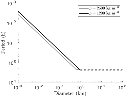
Figure 2: Limiting rotation period for two different densities computed using a bulk cohesion of $100$ Pa.

When the rotation period becomes smaller than $P_{\text{crit}}$ we assume that a fission event takes place, and we re-initialize the spin state. In this process, we do not simulate the production of a binary system, and we assume that the mass lost is small enough to not significantly change the equivalent diameter of the object. During the fission event, we assume the obliquity $\gamma$ to be unchanged. On the other hand, the spin rate is decreased according to the momentum carried away by the ejected mass (see Pravec et al. 2010), and it is given by

$$\omega^{2}_{\text{new}}=\omega^{2}_{\text{old}}-kq.$$ (9)

In Eq. (9), $k=(20\pi G/6)\times(2000\text{ kg m}^{-3})$ is a constant (see the Supplementary Material of Pravec et al. 2010), and $q$ is the mass ratio of the ejected mass to the asteroid mass. The mass ratio $q$ is chosen randomly at each fission event in the range 0.002-0.2, in such a way that $\log q$ is uniformly distributed.

Statler (2009) evaluated how the YORP effect changes when adding boulders on the surface of an asteroid. The author indicated that the torques are affected by the distribution of both small and large boulders, and that a single large boulder can already seriously change the YORP effect. During a spin-up event, boulders can experience landslide or fission, and these phenomena all contribute in changing the torques. For these reasons, during a fission event we also select new functions $f,g$ as described in Sec. 4.1.

It is important to remark that small-scale surface features of sub-kilometer rubble-pile asteroids are largely dominated by boulders. This was already discovered by the JAXA Hayabusa mission on asteroid Itokawa (Michikami et al. 2008), and it has been confirmed more recently by the NASA OSIRIS-REx and the JAXA Hayabusa2 missions on the carbonaceous asteroids Bennu and Ryugu (Lauretta et al. 2019, Watanabe et al. 2019). Moreover, the presence of boulders seems to be independent from the spectral type. It is not clear yet whether these surface features are preserved at sizes smaller than about 150 meters in diameter or not, especially when the rotation is very fast. Theoretical models by Sánchez and Scheeres (2020) suggest that gravel and boulders can survive on the surface of small monolithic fast rotators. Additionally, estimations of thermal inertia on the small super-fast rotator (499998) 2011 PT (Fenucci et al. 2021) suggest either a regolith covering or a rubble-pile structure. These works indicate that the re-shaping assumption at fast rotation may be a good choice even at diameters smaller than 150 meters.

5 STOCHASTIC YORP EFFECT

The YORP effect model of Sec. 4 is also referred to as a static YORP model by Bottke et al. (2015). The analysis on the sensitivity of the YORP effect on small-scale surface features performed by Statler (2009) suggested that the spin evolution could be stochastic rather than deterministic, and this hypothesis has been supported later by hard-sphere discrete element numerical simulations by Cotto-Figueroa et al. (2015). A simpler stochastic YORP model has also been introduced by Bottke et al. (2015). Thermal torques dramatically depend on the surface distribution of both boulders and craters. However, these two distributions are not steady with time. Boulders can migrate by the effect of spinning-up, while their size distribution is changed by cracking induced by micro-meteoroid impacts (Horz and Cintala 1996), and by thermal effects (Delbó et al. 2014). During the artificial impact experiment performed by the Hayabusa2 mission on asteroid Ryugu, a 2 kg copper projectile was shot at 2 km s^-1. It created a $\sim$15 m class crater (Arakawa et al. 2020), demonstrating that impacts could significantly contribute to form craters on rubble-piles and to move boulders across the surface. Additionally, close encounters with planets could also modify the overall shape of the body by the effect of tides (Richardson et al. 1998, Kim et al. 2021). These small and large-scale alterations in shape contribute to a stochastic change of the spin-axis evolution onto a new set of YORP curves. Therefore, the assumption that the thermal torques remain constant during an entire YORP cycle made in Sec. 4 is not valid anymore, but on the contrary, they should change with a shorter timescale.

To implement the stochastic YORP model, we use an approach similar to Bottke et al. (2015). A size-dependant timescale $\tau_{\text{YORP}}(D)$ is introduced, and the torques $f,g$ are changed after a time $\tau_{\text{YORP}}(D)$ has passed, without modifying the spin state. Using estimates on the characteristic timescale of cratering events, Bottke et al. (2015) found a value of $\tau_{\text{YORP}}=1$ My for asteroids with size $D\sim 4$-$8$ km. In the same work, the authors adopted $\tau_{\text{YORP}}=0.5$ My for asteroid (175706) 1996 FG3 ($D=1.9$ km), and $\tau_{\text{YORP}}=0.25$ My for asteroid Ryugu ($D=0.89$ km). Since the collision re-orientation timescale of Eq. (7) depends on the diameter with an exponent of $\beta_{2}=4/3$, and these collisions generally change the shape, we assume for $\tau_{\text{YORP}}$ the same size dependency. Therefore, in our code we use

$$\tau_{\text{YORP}}(D)=0.25\text{ My}\times\bigg{(}\frac{D}{1\text{ km}}\bigg{)}^{4/3}\times c_{\text{stoc}},$$ (10)

where $c_{\text{stoc}}$ is a parameter that can be used to take into account the uncertainties on this timescale, and it can be specified in input. To roughly match the values used by Bottke et al. (2015), we suggest to set this parameter to $c_{\text{stoc}}=0.75$.

At size of $\sim$1 km, this timescale is several factor smaller than the YORP cycle timescale, so that 6-10 re-shaping events are expected during a whole cycle. As the size decreases, the YORP cycle timescale scales as $D^{2}$, while $\tau_{\text{YORP}}$ of Eq. (10) scales as $D^{4/3}$, meaning that there may be a limiting diameter below which the stochastic YORP does not introduce drastic changes in the spin-axis evolution. However, it is not clear yet whether the trend in $\tau_{\text{YORP}}$ is valid down to sizes of  10 m in diameter or not, and this requires more investigation in the future.

In the higher conductivity case $K=0.01$ W m^-1 K^-1, the stochastic YORP does not modify the asymptotic obliquity states, and objects are driven towards 0 or 180 deg. On the other hand, the sign of $f$ at 0/180 deg randomly changes at each stochastic event, meaning that the rotation could either slow down or speed up. This has the effect that the rotation rate $\omega$ evolves as a random-walk process, which generally increases the timescale of the YORP cycle. In the lower case $K=0.001$ W m^-1 K^-1, there is a 20% probability to choose function $g$ with 90 deg as asymptotic obliquity, that is reached by slowing down the rotation. Therefore, here the spin-axis evolution could be even more complicated, since also the obliquity $\gamma$ may behave as a random-walk process as well.

6 TESTS

In this section, we provide some tests of the developed codes. First, we show that the integrations performed with mercury and orbit9 produce results that are in excellent agreement. Later, we provide some tests to show how the static and stochastic YORP models behave.

6.1 mercury vs. orbit9: single object comparison

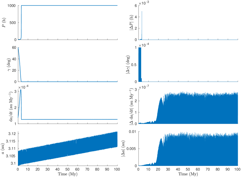
Figure 3: Parameters evolution of the test particle with diameter $D=2$ km, for the conductivity case $K=0.01$ W m^-1 K^-1. The left column shows, from the top to the bottom, the evolution of the rotation period $P$, the obliquity $\gamma$, the semi-major axis drift $\text{d}a/\text{d}t$, and the semi-major axis $a$. The right column shows the evolution of the absolute difference between these quantities obtained with mercury and orbit9.

We first perform a test to verify that the coupled Yarkovsky/YORP effect implementations of mercury and orbit9 give consistent results. We integrated the dynamics of 6 test particles for 100 My, taking into account only the gravitational attraction of Jupiter, Saturn, Uranus, and Neptune. The initial orbit of the particles has a semi-major axis of 3.1 au, a low eccentricity of 0.01, and an inclination of 1 deg, so that possible chaotic effects are limited. The sizes were set to $D=2,1$ and $0.5$ km, and we used two different values of thermal conductivity, namely $K=0.001,0.01$ W m^-1 K^-1. We assumed an initial obliquity of $60$ deg and an initial rotation period of $8$ h for all the objects. Moreover, we used a density of $1200$ kg m^-3, heat capacity of $800$ J m^-1 K^-1, and values of absorption coefficient and emissivity equal to $1$. We chose the MVS integration method for the simulations performed with mercury, and the multi-step integration method for the simulations carried on with orbit9. For both of them, we used a constant time step of 5 days for the orbital evolution and a constant time step $\Delta t_{\text{spin}}=50$ yr for the spin-axis evolution.

To make a coherent comparison between the evolution obtained with the two different packages, we forced the torques $f$ and $g$ to be equal to the mean torques (see Fig. 1, solid black line). We also switched off all the re-orientations and re-shaping events described in Sec. 4 and 5. In this manner, the spin-axis stops evolving when an end-state is reached.

The left column of Fig. 3 shows the time evolution of the rotation period $P$, the obliquity $\gamma$, the semi-major axis drift $\text{d}a/\text{d}t$, and the semi-major axis $a$, for the asteroid with $D=2$ km and $K=0.01$ W m^-1 K^-1. The rotation of this object is slowed down until it reaches a period of 1000 h, while the obliquity evolves towards 0 deg. The asymptotic state is reached after about 3.5 My of evolution. The semi-major axis drift increases during the first period of evolution by the effect of the obliquity moving towards an extreme value. Then it suddenly drops by the effect of the increasing rotation period. In the bottom panel, we can appreciate the increasing trend of the semi-major axis $a$.

The right column of Fig. 3 shows the absolute differences $|\Delta P|,|\Delta\gamma|,|\Delta\text{d}a/\text{d}t|,|\Delta a|$ between the evolution computed with mercury and the one computed with orbit9. From these plots, we can appreciate that the results obtained with the two packages are in good agreement. Indeed, the maximum difference in the rotation period is of the order of $10^{-3}$ h, and $10^{-4}$ deg in obliquity. The difference in the semi-major axis is smaller than $10^{-3}$ au during the first $\sim$17 My evolution, while it grows larger after 20 My, though never exceeding 0.01 au. However, these differences after 20 My may be caused either by long-term integration errors, by the fact that the integration method for the orbital evolution is not the same, or by some small chaotic and diffusion effects. Differences in the rotational dynamics do not play a role here because the spin-axis has already reached the end-state at this point of evolution. Finally, the difference in the semi-major axis drift is of the order of $10^{-7}$ au My^-1, which is orders of magnitude smaller than the typical drifts of km-sized asteroids and smaller.

Similar results were obtained for the other 5 test particles and therefore are not reported here. These tests show that the two implementations produce compatible results, and therefore they can be considered equivalent.

6.2 mercury vs. orbit9: static and stochastic YORP models

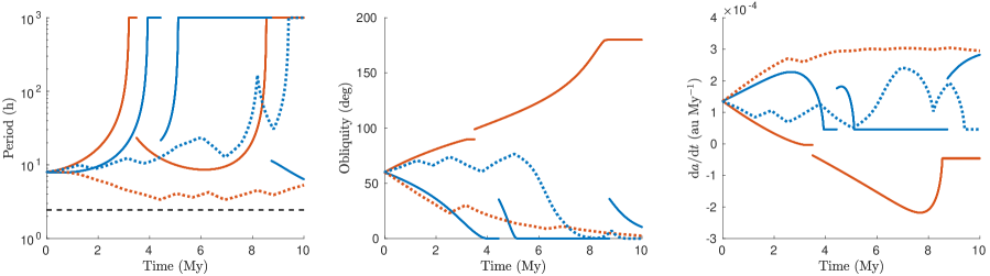
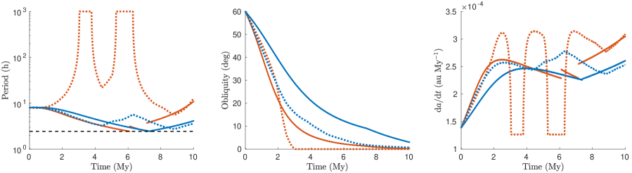
Figure 4: Evolution of rotation period $P$ (left panel), obliquity $\gamma$ (central panel), and semi-major axis drift $\text{d}a/\text{d}t$ (right panel), obtained with different integrators and different YORP models. Red color corresponds to the mercury integrator, while blue color to the orbit9 integrator. Solid curves represent the simulations performed with the static YORP model, while dotted curves those with the stochastic YORP model. The diameter of the asteroid was assumed to be $D=2$ km. The black dashed line in the plots of the first column indicates the critical rotation period. The top row refers to results obtained for conductivity $K=0.001$ W m^-1 K^-1, while the bottom row to $K=0.01$ W m^-1 K^-1.

We performed a second test to understand how the static and the stochastic YORP models behave. We used the same set of 6 asteroids used in Sec. 6.1, with same initial conditions and physical parameters. We integrated the orbits for 10 My with both packages, one time using the static YORP model of Sec. 4, and another time using the stochastic YORP model of Sec. 5.

Figure 4 shows the evolution of the rotation period $P$, the obliquity $\gamma$, and the semi-major axis drift $\text{d}a/\text{d}t$ obtained for the objects with diameter $D=2$ km.

The top row corresponds to the results obtained for $K=0.001$ W m^-1 K^-1. Here, it can be noted that the two objects integrated with the static YORP model (solid curves) both undergo collisional re-orientation when the period becomes large, hence the two packages behave correctly in this respect. When a collisional re-orientation occurs the obliquity value changes randomly, and it can happen that the semi-major axis drift changes the sign (see the red solid curve in the top right panel), thus decreasing the overall effect of the Yarkovsky drift. Note that the timescale of the YORP cycle for these two objects is about 3-4 My. On the other hand, the integrations obtained with the stochastic YORP model (dotted curves) both present other interesting features. In the evolution obtained with mercury (red dotted curve), the obliquity $\gamma$ inverts the trend two times by effect of the occurrence of stochastic events that change the sign of the torque $g$. However, in the overall evolution $\gamma$ is slowly approaching 0 deg. The rotation period $P$ follows a random-walk, and it does not exceeds 10 hours. This has the effect of maximizing the semi-major axis drift $\text{d}a/\text{d}t$ on the 10 My evolution, as can be seen from the top right panel of Fig. 4. In the evolution obtained with orbit9 (blue dotted curve), the obliquity $\gamma$ undergoes several inversions of trend that produce a random walk during the first 5 My, resulting in an evolution narrowed to a limited range. These alternating random obliquity inversions have been found also in the model by Cotto-Figueroa et al. (2015), and the phenomenon is referred to as self-governing YORP. After this period, $\gamma$ finally decreases toward 0 deg. The rotation period has a random-walk evolution as well, and it becomes larger and larger near 10 My, going toward the completion of one YORP cycle. In both cases, the YORP cycle timescale is comparable to the whole 10 My timespan, that is significantly larger than the timescale obtained in the static YORP model.

The bottom row of Fig. 4 shows the evolution of the same object, obtained for a conductivity of $K=0.01$ W m^-1 K^-1. In all the four presented cases, the obliquity $\gamma$ approached the asymptotic value of 0 deg. Here, in the simulations performed with the static YORP model (solid curves) the period is decreasing, and both objects approach the critical spin limit of 2.44 h. When this critical value is reached, a mass shedding event occurs, and indeed we can notice a sudden change in the period. This happens with both mercury and orbit9, confirming that the two packages behave correctly during the spin-up events. Therefore, the YORP cycle for these two evolution ends at fast rotation, and the timescale are comparable to those obtained in the case $K=0.001$ W m^-1 K^-1. In the mercury evolution obtained with the stochastic model (red dotted curve), the object reaches the 1000 h upper limit for the period twice, while the obliquity reaches 0 deg already during the first spin-down event. However, no jumps in $P$ and $\gamma$ due to collision re-orientation events are present. This is also an effect of the stochastic YORP model. As the period is freezed to the upper limit value, a torque $f$ that is negative at 0 deg is selected during a stochastic event. On the other hand, the torque $g$ cannot change sign in this conductivity case. Since the object already reached the extreme obliquity value at the time the stochastic event occurred, the change of sign in $f$ makes the period start evolving again, this time towards lower values. In the orbit9 integration obtained with the stochastic model (blue dotted curve), the obliquity is slowly approaching 0 deg, while the rotation period randomly walks at values smaller than 10 h. This has the effect of maintaining a fairly constant semi-major axis drift of $2.5$-$2.7\times 10^{-4}$ au My^-1 for a significant fraction of the evolution. Again, in both cases the timescale of the YORP cycle is significantly larger than the one obtained in the static YORP model.

These examples already show that, as expected, the stochastic YORP model increases the YORP cycle timescale, and that the semi-major axis drift could be significantly larger than that in the static YORP model.

6.3 Evolution of an asteroid population

To better understand the difference in the outcome between the static and the stochastic YORP models, we performed a test with a larger sample of asteroids. For this purpose, we took the nominal orbit of asteroid (163) Erigone, which is the parent body of the corresponding asteroid family. We used the AstDyS service to get the orbit determined at time 59200 MJD, and we propagated the dynamics of 120 clones for 100 My. We assumed the same initial orbit for all the clones, changing only the physical and spin parameters. We assumed a fixed value of $\rho=1200$ kg m^-3 for the density, that is compatible with carbonaceous C-type asteroids. We fixed the heat capacity to $C=800$ J m^-1 K^-1, and the thermal conductivity to $K=0.01$ W m^-1 K^-1. The initial rotation period was fixed to 6 h, while the obliquity was randomly generated according to a uniform distribution for $\cos\gamma$ between -1 and 1. On the other hand, the diameter $D$ was randomly generated between 1 and 5 km. Numerical integrations were performed with the MVS method for mercury and with the multistep method for orbit9, using 5 days time step for the orbital dynamics and 50 yr time step for the spin-axis dynamics.

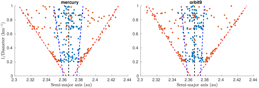
Figure 5: Final osculating semi-major axis vs. inverse of diameter of the 120 clones, for mercury (left panel) and orbit9 (right panel). Blue dots are the results obtained with the static YORP model, while red dots are obtained with stochastic YORP model. The vertical dashed black line indicates the initial semi-major axis, while the dashed blue and red lines are the fits of the V-shapes.

Table 1: Parameters of the V-shape fits.

	mercury		orbit9
V-shape side	$\alpha$	$\beta$	$\alpha$	$\beta$
IN (stochastic)	2.3637$\pm$0.0023	-0.0588$\pm$0.0035	2.3617$\pm$0.0061	-0.0527$\pm$0.0095
OUT (stochastic)	2.3722$\pm$0.0056	-0.0562$\pm$0.0087	2.3705$\pm$0.0023	-0.0607$\pm$0.0036
IN (static)	2.3599$\pm$0.0020	-0.0116$\pm$0.0031	2.3582$\pm$0.0039	-0.0081$\pm$0.0061
OUT (static)	2.3767$\pm$0.0014	-0.0076$\pm$0.0022	2.3740$\pm$0.0027	-0.0048$\pm$0.0041

We propagated the set of clones the first time with the static YORP model, and the second time with the stochastic YORP model. Figure 5 shows the final osculating semi-major axis versus the inverse of the diameter for both packages. From these plots, it can be noted that the asteroids integrated with the static YORP model (blue dots) are less dispersed from the initial semi-major axis value. Although an object may be affected by a larger semi-major axis drift (compare for instance with Fig. 3 and 4) for a while, the average drift is slowed down by the effect of collisional re-orientations happening at long rotation period. When such events happen, the obliquity could significantly change, making the drift $\text{d}a/\text{d}t$ suddenly change sign (see also the solid red curve of the top right panel in Fig. 4), hence decreasing the overall Yarkovsky effect.

The objects propagated using the stochastic YORP model (red dots) are much more dispersed in the semi-major axis. Moreover, even though this test does not represent an entirely consistent simulation of the evolution of an asteroids family, a strong correlation with the diameter can be noticed in the two panels of Fig. 5, and the typical V-shape can be recognized. These results mean that the YORP cycle timescale is generally increased with the stochastic YORP model, as we have already seen in the examples of Fig. 4. Thus, objects can maintain a faster Yarkovsky drift for longer, drifting further from the initial semi-major axis value.

To further test whether the two packages provide the same statistical results, we fitted the edges of the V-shape. This was performed with a linear model of the form $a=\alpha+\beta D^{-1}$, using a least-square method described in Milani et al. (2014). The obtained numerical values are reported in Table 1. The fits of the V-shape for the simulations performed with mercury and orbit9 agree within the error at 1-$\sigma$ level, for both the static and the stochastic YORP models, providing evidence that the two packages produce the same results, at least in the context of main-belt asteroids.

7 SUMMARY AND CONCLUSIONS

In this paper, we presented modified versions of the mercury and orbfit numerical integration packages that take into account thermal effects acting on small Solar System bodies. The Yarkovsky effect is computed with an analytical model and then added to the gravitational vector field as a non-conservative force along the tangential direction. The YORP effect governs the spin-axis dynamics of the object, and it is integrated along with the orbital integration. We implemented a static and a stochastic YORP model, which are both based on statistical studies performed by Čapek and Vokrouhlický (2004). Finally, we first provided some tests to show that the two modified packages provide comparable results. Then we presented some simulations to show how the two different YORP models behave.

The modified versions of the mercury and orbfit packages developed in this paper are publicly available. They are suitable for statistical studies of the dynamics of large sets of asteroids. For instance, these packages can be potentially used to investigate how the combined Yarkovsky/YORP effects affect the dispersion and the age estimation of asteroid families (see e.g. Marzari et al. 2020, Dell’Oro et al. 2021), or to clarify the origin and formation process of the so-called YORP-eye (Paolicchi and Knežević 2016). Additionally, it can be used to test how the migration of small asteroids from the main-belt to the near-Earth region changes with the introduction of the YORP effect in the dynamics (Granvik et al. 2017).

Finally, we point out that the solution adopted here for modeling the YORP effect is not the only possible one, and the understanding of this thermal effect is still a matter of research (see Vokrouhlický et al. 2015, and references therein). Other models have been developed in recent years. For instance, Nesvorný and Vokrouhlický (2007), Scheeres and Mirrahimi (2008) developed analytical models based on spherical harmonics, while Golubov and Krugly (2012), Golubov (2017) found that the re-emission of the heat of small boulders causes a torque component parallel to the surface, that is known as the tangential YORP effect. When this component is added to the torques, new rotational equilibria at which $P$ and $\gamma$ remain constant arise (Golubov and Scheeres 2019, Golubov et al. 2021). Although we designed the code so that changing the YORP effect model is not technically complex, we leave these tasks for future developments of the software.

Acknowledgements – We thank Aldo Dell’Oro for the referee report that helped us to improve the paper. The authors have been supported by the MSCA ETN Stardust-R, Grant Agreement n. 813644 under the European Union H2020 research and innovation program. BN also acknowledges support by the Ministry of Education, Science and Technological Development of the Republic of Serbia, contract No. 451-03-68/2022-14/200104.

References

- Arakawa et al. (2020) Arakawa, M., Saiki, T., Wada, K., et al. 2020, Science, 368, 67
- Bolmont et al. (2015) Bolmont, E., Raymond, S. N., Leconte, J., Hersant, F., and Correia, A. C. M. 2015, A&A, 583, A116
- Bottke et al. (2006) Bottke, William F., J., Vokrouhlický, D., Rubincam, D. P., and Nesvorný, D. 2006, Annual Review of Earth and Planetary Sciences, 34, 157
- Bottke et al. (2002) Bottke, W. F., Morbidelli, A., Jedicke, R., et al. 2002, Icar, 156, 399
- Bottke et al. (2015) Bottke, W. F., Vokrouhlický, D., Walsh, K. J., et al. 2015, Icar, 247, 191
- Brož et al. (2011) Brož, M., Vokrouhlický, D., Morbidelli, A., Nesvorný, D., and Bottke, W. F. 2011, MNRAS, 414, 2716
- Bulirsch and Stoer (2002) Bulirsch, R. and Stoer, J. 2002, Introduction to Numerical Analysis, 3rd edn., Texts in Applied Mathematics 12 (Springer New York)
- Carpino et al. (1987) Carpino, M., Milani, A., and Nobili, A. M. 1987, A&A, 181, 182
- Chambers (1999) Chambers, J. E. 1999, MNRAS, 304, 793
- Chambers and Migliorini (1997) Chambers, J. E. and Migliorini, F. 1997, in AAS/DPS Meeting Abstracts #29, AAS/Division for Planetary Sciences Meeting Abstracts, 27.06
- Cotto-Figueroa et al. (2015) Cotto-Figueroa, D., Statler, T. S., Richardson, D. C., and Tanga, P. 2015, ApJ, 803, 25
- Del Vigna et al. (2019) Del Vigna, A., Roa, J., Farnocchia, D., et al. 2019, A&A, 627, L11
- Delbó et al. (2014) Delbó, M., Libourel, G., Wilkerson, J., et al. 2014, Nature, 508, 233
- Dell’Oro et al. (2021) Dell’Oro, A., Boccenti, J., Spoto, F., Paolicchi, P., and Knežević, Z. 2021, MNRAS, 506, 4302
- Dermott et al. (2021) Dermott, S. F., Li, D., Christou, A. A., et al. 2021, MNRAS, 505, 1917
- -Došović et al. (2020) -Došović, V., Novaković, B., Vukotić, B., and Ćirković, M. M. 2020, MNRAS, 499, 4626
- Everhart (1985) Everhart, E. 1985, An efficient integrator that uses Gauss-Radau spacings, Vol. 115 (Dynamics of Comets: Their Origin and Evolution, Springer), 185
- Farinella and Vokrouhlicky (1999) Farinella, P. and Vokrouhlicky, D. 1999, Science, 283, 1507
- Farinella et al. (1998) Farinella, P., Vokrouhlický, D., and Hartmann, W. K. 1998, Icar, 132, 378
- Fenucci and Novaković (2021) Fenucci, M. and Novaković, B. 2021, AJ, 162, 227
- Fenucci et al. (2021) Fenucci, M., Novaković, B., Vokrouhlický, D., and Weryk, R. J. 2021, A&A, 647, A61
- Golubov (2017) Golubov, O. 2017, AJ, 154, 238
- Golubov and Krugly (2012) Golubov, O. and Krugly, Y. N. 2012, ApJL, 752, L11
- Golubov and Scheeres (2019) Golubov, O. and Scheeres, D. J. 2019, AJ, 157, 105
- Golubov et al. (2021) Golubov, O., Unukovych, V., and Scheeres, D. J. 2021, AJ, 162, 8
- Granvik et al. (2017) Granvik, M., Morbidelli, A., Vokrouhlický, D., et al. 2017, A&A, 598, A52
- Grimm and Stadel (2014) Grimm, S. L. and Stadel, J. G. 2014, ApJ, 796, 23
- Hairer and Wanner (1996) Hairer, E. and Wanner, G. 1996, Solving Ordinary Differential Equations II: Stiff and Differential-Algebraic Problems, 2nd edn., Springer Series in Computational Mathematics 14 (Springer-Verlag Berlin Heidelberg)
- Holsapple (2007) Holsapple, K. A. 2007, Icar, 187, 500
- Horz and Cintala (1996) Horz, F. and Cintala, M. J. 1996, Meteoritics and Planetary Science Supplement, 31, A65
- Hsieh et al. (2020) Hsieh, H. H., Novaković, B., Walsh, K. J., and Schörghofer, N. 2020, AJ, 159, 179
- Hu et al. (2021) Hu, S., Richardson, D. C., Zhang, Y., and Ji, J. 2021, MNRAS, 502, 5277
- Kim et al. (2021) Kim, Y., Hirabayashi, M., Binzel, R. P., et al. 2021, Icar, 358, 114205
- Knežević (2020) Knežević, Z. 2020, MNRAS, 497, 4921
- Knežević and Milani (2000) Knežević, Z. and Milani, A. 2000, Celestial Mechanics and Dynamical Astronomy, 78, 17
- Lauretta et al. (2019) Lauretta, D. S., Dellagiustina, D. N., Bennett, C. A., et al. 2019, Natur, 568, 55
- Levison and Duncan (1994) Levison, H. F. and Duncan, M. J. 1994, Icar, 108, 18
- Marsden et al. (1973) Marsden, B. G., Sekanina, Z., and Yeomans, D. K. 1973, AJ, 78, 211
- Martin and Livio (2021) Martin, R. G. and Livio, M. 2021, MNRAS, 506, L6
- Marzari et al. (2020) Marzari, F., Rossi, A., Golubov, O., and Scheeres, D. J. 2020, AJ, 160, 128
- Michikami et al. (2008) Michikami, T., Nakamura, A. M., Hirata, N., et al. 2008, Earth, Planets, and Space, 60, 13
- Milani et al. (2014) Milani, A., Cellino, A., Knežević, Z., et al. 2014, Icar, 239, 46
- Milani and Nobili (1988) Milani, A. and Nobili, A. M. 1988, Celestial Mechanics, 43, 1
- Muinonen (1998) Muinonen, K. 1998, A&A, 332, 1087
- Murray and Dermott (2000) Murray, C. D. and Dermott, S. F. 2000, Solar System Dynamics, 1st edn. (Cambridge University Press)
- Nesvorný and Vokrouhlický (2007) Nesvorný, D. and Vokrouhlický, D. 2007, AJ, 134, 1750
- Nobili et al. (1989) Nobili, A. M., Milani, A., and Carpino, M. 1989, A&A, 210, 313
- Novaković et al. (2015) Novaković, B., Maurel, C., Tsirvoulis, G., and Knežević, Z. 2015, ApJL, 807, L5
- Paolicchi and Knežević (2016) Paolicchi, P. and Knežević, Z. 2016, Icar, 274, 314
- Pavela et al. (2021) Pavela, D., Novaković, B., Carruba, V., and Radović, V. 2021, MNRAS, 501, 356
- Pravec and Harris (2000) Pravec, P. and Harris, A. W. 2000, Icar, 148, 12
- Pravec et al. (2002) Pravec, P., Harris, A. W., and Michalowski, T. 2002, Asteroid Rotations (Asterois III, University of Arizona Press), 113–122
- Pravec et al. (2010) Pravec, P., Vokrouhlický, D., Polishook, D., et al. 2010, Natur, 466, 1085
- Rein and Liu (2012) Rein, H. and Liu, S. F. 2012, A&A, 537, A128
- Richardson et al. (1998) Richardson, D. C., Bottke, W. F., and Love, S. G. 1998, Icar, 134, 47
- Roa et al. (2021) Roa, J., Farnocchia, D., and Chesley, S. R. 2021, AJ, 162, 277
- Sánchez and Scheeres (2018) Sánchez, P. and Scheeres, D. J. 2018, Progress in Earth and Planetary Science, 5, 5
- Sánchez and Scheeres (2020) Sánchez, P. and Scheeres, D. J. 2020, Icar, 338, 113443
- Scheeres (2007) Scheeres, D. J. 2007, Icar, 188, 430
- Scheeres and Mirrahimi (2008) Scheeres, D. J. and Mirrahimi, S. 2008, Celestial Mechanics and Dynamical Astronomy, 101, 69
- Spitale and Greenberg (2001) Spitale, J. and Greenberg, R. 2001, Icar, 149, 222
- Spoto et al. (2015) Spoto, F., Milani, A., and Knežević, Z. 2015, Icar, 257, 275
- Statler (2009) Statler, T. S. 2009, Icar, 202, 502
- Tamayo et al. (2020) Tamayo, D., Rein, H., Shi, P., and Hernandez, D. M. 2020, MNRAS, 491, 2885
- Čapek and Vokrouhlický (2004) Čapek, D. and Vokrouhlický, D. 2004, Icar, 172, 526
- Vokrouhlický (1998) Vokrouhlický, D. 1998, A&A, 338, 353
- Vokrouhlický (1999) Vokrouhlický, D. 1999, A&A, 344, 362
- Vokrouhlický et al. (2007) Vokrouhlický, D., Breiter, S., Nesvorný, D., and Bottke, W. F. 2007, Icar, 191, 636
- Vokrouhlický et al. (2006) Vokrouhlický, D., Brož, M., Bottke, W. F., Nesvorný, D., and Morbidelli, A. 2006, Icar, 182, 118
- Vokrouhlický and Čapek (2002) Vokrouhlický, D. and Čapek, D. 2002, Icar, 159, 449
- Vokrouhlický et al. (2015) Vokrouhlický, D., Bottke, W. F., Chesley, S. R., Scheeres, D. J., and Statler, T. S. 2015, The Yarkovsky and YORP Effects (Asteroids IV, University of Arizona Press), 509–532
- Watanabe et al. (2019) Watanabe, S., Hirabayashi, M., Hirata, N., et al. 2019, Science, 364, 268
- Wisdom et al. (1996) Wisdom, J., Holman, M., and Touma, J. 1996, Fields Institute Communications, 10, 217
- Zhang and Gladman (2022) Zhang, K. and Gladman, B. J. 2022, NewA, 90, 101659
- Zhang et al. (2021) Zhang, Y., Michel, P., Richardson, D. C., et al. 2021, Icar, 362, 114433