Instant Loans Can Lift Subjective Well-Being:
A Randomized Evaluation of Digital Credit in Nigeria

Abstract

Digital loans have exploded in popularity across low- and middle-income countries, providing short term, high interest credit via mobile phones. This paper reports the results of a randomized evaluation of a digital loan product in Nigeria. Being randomly approved for digital credit (irrespective of credit score) substantially increases subjective well-being after an average of three months. For those who are approved, being randomly offered larger loans has an insignificant effect. Neither treatment significantly impacts other measures of welfare. We rule out large short-term impacts – either positive or negative – on income and expenditures, resilience, and women’s economic empowerment.

Keywords: Digital credit, digital loan, subjective well-being, mobile money, Nigeria

JEL classification: O16, O30, O55

1 Introduction

Over the last several years, “digital loans” have transformed the consumer credit landscape in developing countries. These products, which allow individuals with no formal financial history to access small loans via a mobile phone, have become enormously popular. In Kenya, a 2018 survey indicated that 27% of all adults had an outstanding digital credit loan — much higher than the number who had microfinance loans ($<5\%$) (Totolo, 2018). In Nigeria, despite the low penetration of formal financial services, over 50 different companies currently offer digital loan products.

In principle, increased access to credit could have positive effects for both households and small enterprises. Despite the strong demand for these loans, critics argue that they may not improve borrowing well-being, since loan terms are opaque and may induce borrowers to fall deep into debt (Donovan and Park, 2019). Interest rates are high – typically from 138% to over 1000% APR (Francis et al., 2017) – and are accompanied by high rates of default (Johnen et al., 2021). Many have criticised providers for using predatory practices on people with little experience with formal financial products (Hindenburg Research, 2020). The debate around digital credit in developing countries echoes that surrounding payday lending in wealthy nations, but with higher stakes: these loans are in many cases the only source of formal credit available to billions of people, many of whom live near subsistence levels with little social safety net to fall back on.

This paper presents the results of the first randomized controlled trial to assess the welfare impacts of digital loans. In partnership with a large Financial Services Provider (FSP) in Nigeria, we increased the availability of credit to a random subset of new loan applicants. Some loan applicants who would normally have been denied credit were approved; some loan applicants were randomly offered larger initial loans than they would have otherwise received. After roughly three months, we surveyed 1,618 individuals by phone to study the welfare impact of increased access to digital credit.

Following a pre-registered pre-analysis plan, our analysis produces several results. First, as expected, being auto-approved for a digital loan increased use of formal credit, as measured several months after the initial loan application. Borrowing from the FSP increases by $30 USD ($86 PPP) on average. We observe modest substitution away from informal sources of credit, and a statistically insignificant increase in financial health, measured using a standardized 14-question financial health index. For our second treatment, for each dollar increase in the value of the initial loan offer, borrowing from the FSP increases by a total of $1.24 ($3.50 PPP) across all loans.

Second, being auto-approved for digital credit substantially increases subjective well-being, by 0.281 standard deviations. This effect is large, even in comparison to the effect of cash transfers and multifaceted antipoverty programs, which are 10-20 times more costly to implement (Ridley et al., 2020). Most of the improvement comes from reduced depression, as measured by a standard survey module (Patient Health Questionnaire or PHQ-9); it is also supported by a statistically insignificant increase in reported life satisfaction. In contrast to the large treatment effects of auto-approval, offering larger loans has only small and statistically insignificant effects on subjective well-being.

Third, we are able to rule out large effects — either positive or negative — on the other key dimensions of welfare that we pre-specified, including income and expenditures, resilience to shocks, and women’s economic empowerment. The absence of significant positive effects may not be surprising given the small size of the initial loan offer (these ranged from roughly $3 to $35); however, the absence of significant negative effects suggests that the widespread concern over the predatory nature of these loans may be not be justified, at least in our context.

In our final set of results, which was not pre-specified, we explore why access to these small, on-demand loans has such a large impact on subjective well-being. Respondents report taking out loans in order to meet short run needs. Although our sample size limits our ability to study heterogeneity, we find suggestive evidence that impacts are greatest for individuals who are unemployed or have low credit scores. While the effects are not significant at traditional levels, when an unemployed and employed applicant are both auto-approved, the magnitude of the differential effect is predicted to be large enough to close the gap in subjective well-being between them. It likewise closes the gap associated with low credit scores. These large effects of providing small amounts of liquidity on demand are consistent with a growing literature that suggests that being unable to access small but critical resources in times of need can be damaging for mental health (Haushofer and Fehr, 2014; Banerjee et al., 2020).

The quantitative results from our RCT are also consistent with the qualitative stated opinions of the company’s customers: 85% of our sample reported that loan terms were fair, and 94% report not regretting taking out a loan from the FSP. Likewise, we do not find evidence of some of the behavioral mistakes that are seen with payday lending. In contrast with Allcott et al. (2021), who find that inexperienced payday lending borrowers in the United States underestimate future borrowing, we find that new applicants actually over-estimate future borrowing: applicants predict they have a 62% chance of borrowing from the partner FSP in the next 30 days on average, but in fact only 42% do.

To summarize: we do not find substantial negative effects on borrowers. The few significant effects we observe are positive, and access to digital credit has a substantial positive effect on subjective well-being. One caveat to this generally positive assessment is that our study focuses on the relatively short-term effects of small loans to new borrowers; we cannot say whether different effects would be observed over longer time horizons to long-term customers.

1.1 Related literature

This paper complements two recent quasi-experimental evaluations of the welfare impacts of digital credit that exploit discontinuities in loan approvals based on credit score. Bharadwaj et al. (2019) finds small but generally positive longer-term effects of digital loans in Kenya, particularly with respect to household resilience to shocks. Brailovskaya et al. (2020) finds some evidence of positive effects on (self-reported) financial well-being from digital loans in Malawi. They also find that giving borrowers additional information about the (high) fees and risks of default increased demand for digital credit.

Our results also relate to a larger literature on the welfare impacts of expanding credit access in low- and middle-income countries. Most relevant to our results, Angelucci et al. (2015) and Fernald et al. (2008) find that access to microfinance reduces depression, though Fernald et al. (2008) also observe it increases stress. We compare our results on subjective well-being to these and other studies in Section 4.4, after presenting our main results. More broadly, empirical studies of credit have highlighted the high returns to capital for small enterprises (de Mel et al., 2008, 2009; Karlan et al., 2014), and heterogeneous impacts on household consumption and welfare (Banerjee et al., 2015; Tarozzi et al., 2015; Attanasio et al., 2015; Crépon et al., 2015; Karlan and Zinman, 2010; Augsburg et al., 2015; Meager, 2019). However, digital loans like we study are different from typical microfinance loans: they are much smaller, can be accessed instantaneously, are shorter-term, and typically charge substantially higher interest rates.

The debate around digital credit also parallels concerns around payday lending in wealthy nations, which also offer repeat, short-term, high-interest rate loans (cf. Bhutta et al., 2015). That literature documents both positive and negative effects on borrowers (Zinman, 2010; Melzer, 2011, 2018; Morse, 2011; Morgan et al., 2012; Carrell and Zinman, 2014; Bhutta et al., 2015, 2016; Gathergood et al., 2019; Skiba and Tobacman, 2019).

2 Setting

Our study population is a random sample of new customers on a popular digital credit platform in Nigeria. Nigeria has relatively high rates of financial inclusion relative to neighboring countries: 51% of adults report using formal financial services (EFInA, 2021). An estimated 89% of Nigerians own a mobile phone and 28% of adults report using digital financial services (EFInA, 2021).

2.1 The digital credit product

Our study examines the welfare impacts of small loans offered by a private financial service provider (FSP) in Nigeria. Consumers can apply for loans via a smartphone application, and the FSP assesses creditworthiness using behavioral data derived from their smartphone (as in Björkegren and Grissen, 2020). Approved applicants are presented with a menu of three loan offers of different value. Applicants must have a bank account to register, but do not need a formal financial history.

In general, loans range from 1,000 Nigerian Naira (NGN), or roughly USD $2.60, to 200,000 NGN (USD $528). Loans are typically due after 28 days, and the interest rates we observe range from 15% – 22% per month (implying an annual percentage rate of 195% to 287%). If a borrower does not repay on time, the FSP does not charge a late fee, but if a customer defaults, they are not eligible to apply for future loans from the FSP. If a customer repays, they gradually become eligible for larger loans.

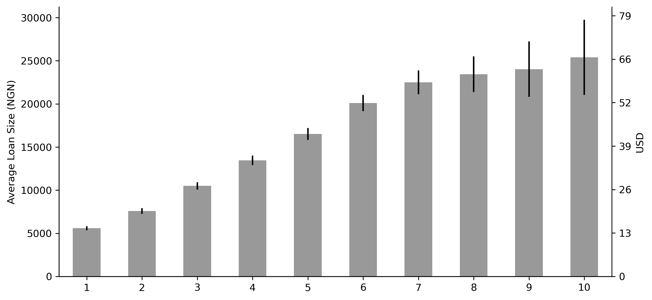
Figure A1: Loan Ladder

In our study sample (N=1,618), the average initial loan amount is approximately NGN 5,600 ($15); over the roughly 3 months between enrolment and survey, average total borrowing is NGN 21,300 ($56). Appendix Figure A1 shows how loan values increase as customers repay prior loans. 7% of the loans taken out within our sample end in default, and altogether 23% of borrowers default at least once.

The product we examine is broadly similar to other digital credit products offered across sub-Saharan Africa (Francis et al., 2017). In particular, it is similar to the M-Shwari loan product in Kenya analyzed in Bharadwaj et al. (2019), and the Kutchova product in Malawi analyzed in Brailovskaya et al. (2020), though our FSP’s loans tend to be slightly larger.

2.2 Descriptive evidence

Qualitative surveys suggest that borrowers like the FSP’s product, and demand for loans is high. Among the approved applicants we observe in data from the FSP, 85% take out a loan. Among those surveyed (details on the survey are provided below), 86% report that the FSP’s loan terms are fair and 94% report not regretting taking out a loan from the FSP.

We also look for evidence of the sort of behavioral trap observed with payday loans in Allcott et al. (2021), who find that payday borrowers frequently underestimate future borrowing. However, we find that our borrowers actually over-estimate future borrowing from the FSP (Appendix Figures A2 and A3): the average applicant predicts they have a 62% chance of borrowing from the FSP in the next 30 days, whereas in practice only 42% borrow within that period. As in Allcott et al. (2021), the magnitude of misprediction decreases with experience (measured by the number of FSP loans taken out prior to survey).

3 Experimental design and estimation strategy

As part of a research collaboration with the partner FSP, a randomly-selected sample of the FSP’s applicants were included in a Randomized Controlled Trial (RCT) to measure the impact of digital loans on well-being. This section describes the experimental design, the data we collected, as well as our estimation strategy, all of which were also pre-registered in our Pre-Analysis Plan (AEARCTR-0005029).

3.1 Experimental design

As part of its normal business operations, the partner FSP frequently runs randomized controlled trials (A/B tests). We worked with the FSP to launch a new RCT, which included a randomly selected 8% of all new applicants who installed the app between August 2019 to February 2020. In total, 46,937 people were included in the RCT. These participants were cross-randomized across two different treatment arms:

Auto-Approval Treatment (Extensive Margin)

Half of all participants (4% of all new applicants) were automatically approved for credit, regardless of credit score. The other half (‘standard approval’ group) were approved only if their credit score exceeded a threshold.

Initial Loan Value (Intensive Margin)

Applicants who were approved received a randomly assigned maximum initial loan offer, selected from NGN 1000, 2000, 5000, 10,000, or 13,000 (between about $2.75 and $35.75). Customers who repaid their initial loan on time would subsequently be eligible for future loans according to the FSP’s standard loan ladder.

3.1.1 Subject recruitment, surveys, attrition, and weighting

All 46,937 applicants who installed our partner FSP’s smartphone app during the study period were invited via text message to participate in a phone survey. Those who opted in by responding to the message were then contacted by the research team, and asked for informed consent to participate in a 25-minute phone survey.

Invitations were staggered over time to ensure that we could quickly follow-up with a phone call to the respondent. To ensure that the different treatment arms were balanced across cohorts (defined as the set of applicants who enrolled in a particular week), we sampled approximately 2,000-2,500 consumers to be contacted each week, roughly three months after enrolment. Surveying began in the week of November 11, 2019, and concluded in the week of February 7, 2020. The survey gathered details on demographics, household composition, financial behavior, subjective well-being and household decision making. Respondents were compensated with an airtime incentive of NGN 3600 upon completion.

Our main analysis focuses on the subset of 1,618 consumer who responded to the text message and successfully completed the phone survey. We omit from our analysis 439 people who we surveyed but were ineligible for loans because they were never assigned a credit score (typically because they never opened the app after installation, or their data did not successfully upload). Appendix Table A1 summarizes treatment assignment for individuals in the final sample.

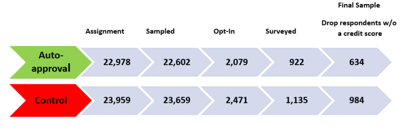
Figure A4: Experimental Design

We weight each survey respondent by the inverse probability of being included in our sample, to address two concerns. First, attrition is slightly higher in the auto-approval group (see Appendix Figure A4). Second, some individuals were not assigned to the standard approval group until slightly later in the enrolment process due to an engineering error. This caused us to survey some of the standard approval group closer to enrolment (3-5 days, on average) than the auto-approval group. We construct probability weights for treatment group interacted with cohort indicators, assuming that consumers who enrolled in a treatment arm in a particular cohort have the same joint probability of being in our final sample. This ensures that the mean weighted distribution of enrolment times are equal.

3.1.2 Sample characteristics and balance

Applicants in our sample are mostly male (76%), around 30 years of age on average, and educated at the secondary school or university level. Respondents are distributed across the various states of Nigeria, with Lagos having the largest share (33%). A majority of respondents are employed in either their own business (41%), or in salaried jobs (39%). For more details, see Appendix Table A2.

Characteristics are balanced across treatment arms (Appendix Table LABEL:balance_table_1618). We test for balance in a number of ways. First, we examine balance between the auto-approval and standard approval group arms for each individual characteristic (column 2). Then, we report the F-stat from a joint test of significance, on all fixed characteristics (column 3). Finally, we test whether the initial loan offer amount is independent of each characteristic (column 6). Overall, we find no significant differences between the average characteristics of the auto-approval and standard approval groups, except for the initial amount offered to applicants in Lagos.

3.2 Estimation strategy

We are interested in understanding how use of digital credit affects the welfare of applicants. Our two randomized treatments $\boldsymbol{Z}_{i}$ create exogenous variation in credit access and use. We estimate the impact of these treatments on each outcome $Y_{i}$ using regressions of the form:

$$\mbox{$Y_{i}$}=\pi_{0}+\boldsymbol{\pi}_{1}\boldsymbol{Z}_{i}+\boldsymbol{\pi}_{2}\boldsymbol{X}_{i}+\nu_{week}+\nu_{enumerator}+\varepsilon_{i}$$ (1)

To reduce sampling variation, we include a vector of controls ($\boldsymbol{X}_{i}$: respondent gender, education, ethnicity, location, age, household size, head of household), and fixed effects for week of enrollment and enumerator ($\nu_{week}$ and $\nu_{enumerator}$). All regressions in our analysis are weighted to be representative of the population of first-time borrowers on the FSP’s platform (as described in Section 3.1.1).

We have two randomized treatments ($\boldsymbol{Z}_{i}$). First: a dummy variable indicating whether the respondent is assigned to the auto-approval group. Since this treatment primarily affects the eligibility of applicants whose credit score would normally disqualify them from receiving a loan, we interact it with dummy variables indicating if the respondent would otherwise had been rejected due to having a credit score below the threshold at the time of enrolment (Auto-approval_i*Under-threshold_i, and Auto-approval_i*Over-threshold_i). Second, the value of the randomly assigned initial loan offer for approved applicants (Initial-offer${}_{i}\in\{1,2,5,10,13\}$, in NGN 1000). To account for baseline differences between those below the threshold, we include the uninteracted control (Under-threshold_i), which is not randomly assigned.

4 Results

Our main analysis highlights three sets of results. First, we show how our two randomized treatments – and in particular the extensive margin that auto-approved loans for applicants with low credit scores – increased borrowing and affected other financial behaviors of applicants. Second, following our pre-analysis plan, we show how increased access to loans affected several pre-specified indices of welfare; while most effects are statistically insignificant, there are large and significant improvements in subjective well-being. Third, we do a deep dive into the subjective well-being results, to better understand where these effects are coming from, and to contextualize them relative to related interventions.

4.1 Impacts on borrowing

The effects of the two randomized treatments on the financial behaviors of applicants are shown in Table 1. The first two rows indicate the effect of the extensive margin treatment, being auto-approved for a loan. We show the effect separately for people below (row 1) and above (row 2) the minimum credit score threshold. The third row indicates the effect of the intensive margin treatment, the randomly assigned initial loan offer.

Broadly, we find that both treatments increase the amount that applicants borrowed from the partner FSP, but that only the extensive margin treatment increases the likelihood that applicants take out any loan. The auto-approval treatment also affects other aspects of financial behavior, but generally only among applicants below the credit score threshold.

In greater detail, the first column of Table 1 reports the effects of both treatments on the total borrowed from the FSP, as observed in administrative data from the FSP, in the period between the initial app installation and the date of the phone survey. For applicants under the threshold at the time of enrollment, auto-approval increases borrowing from FSP by 11,657 NGN ($30, or $86 PPP). The next row indicates that, for applicants above the threshold, auto-approval increased borrowing by a statistically insignificant 1,227 NGN. In the third row, we observe that, for each additional 1,000 NGN offered in the initial loan, borrowing from FSP increases by 1,239 NGN. Since the value of the initial loan ranges from 1,000 to 13,000 NGN, the initial offer treatment induces a predicted difference in borrowing as large as 14,868 NGN. For comparison, individuals in the standard approval group borrow a total of 20,036 NGN on average from the FSP.

The remaining columns of Table 1 indicate the effects on other financial behaviors. In Column 2, we observe that auto-approval increases the proportion of applicants under the threshold who take out any loan by 37 percentage points. This effect is driven by having a loan from the FSP: column 3 indicates that auto-approval does not significantly affect the proportion of applicants with a non-FSP loan. The value of the randomly assigned initial offer has no effect on whether either category of loans are taken out (columns 2 and 3).

Columns 4 and 5 of Table 1 indicate that increased access to digital credit causes applicants to substitute from informal credit towards formal credit. For applicants below the credit score threshold, the auto-approval treatment increased an index of formal borrowing by 0.88 standard deviations and decreased an index of informal borrowing by 0.33 standard deviations. Each index is the average of the z-scores of the number and amount of loans reported taken out in the last 3 months from formal sources (digital credit, bank, microfinance, or cooperative) or informal sources (friends and family, moneylenders, or airtime credit). This substitution away from informal credit is driven by a large reduction in borrowing from friends and family and a small reduction in borrowing from moneylenders — there is no effect of our treatments on the use of other digital lenders, banks, or cooperatives. We see no significant effect of increasing the initial offer on use of informal credit.

Both auto-approval and offer amounts significantly increase the applicant’s ratio of loans taken out to income (both for one month; column 6) – the closest our data will allow us to get to a debt/income ratio. Auto-approval increases loans taken out by 7.9 percentage points of income on average for applicants under the threshold; likewise, each additional 1,000 NGN in the initial loan increases this ratio by 0.005. Relative to the mean ratio of 9.8% of income in standard approval group, these are substantial increases. However, in absolute terms, households have limited use of credit (compare, for instance, to the United States, where the average ratio of household debt payments to income is nearly 100% (Ahn et al., 2018)).

Finally, columns 7-9 indicate that neither treatment had significant effects on the applicant’s self-reported income, expenditures, or savings.

4.2 Welfare impacts

Beyond the direct impacts on borrowing, we evaluate the impact of access to digital credit on several key dimensions of applicant welfare. We focus on four families of outcomes that we pre-registered and pre-specified prior to conducting the endline survey: Financial health, resilience, women’s economic empowerment, and subjective well-being. For each family, we focus on summary indices that aggregate a number of related variables. We standardize each variable by subtracting the mean and dividing by the standard deviation of the standard approval group. We then construct the summary index as the mean of the z-scores of the component variables. In the event that a family has more than one summary index of interest, we report p-values that adjust for multiple hypothesis testing (using the Sidak-Holm adjustment). The impact of our two randomized treatments on these four families of outcome indices are presented in Table 2.

Financial health

Results in column 1 indicate that neither expansion of digital credit had an effect on an index of the overall financial health of the applicant, as measured by the respondent’s answers to 14 standardized questions (Consumer Finance Protection Bureau, 2017). Across the 14 individual questions, the two treatments had generally positive but statistically insignificant effects (Appendix Figure A6).

Resilience

Increased access to digital credit did not significantly impact the applicant’s self-reported coping with negative shocks. Column 2 of Table 2 shows the effect on the applicant’s ability to experience a negative economic shock without forgoing expenditure or adjusting behavior (based on the questions used in Bharadwaj et al. (2019)). Column 3 reports an index of the applicant’s ability to pay a large amount in an emergency and manage without income.

The coefficients on both summary indices are very small and close to zero, and the confidence intervals are fairly tight. We do find some suggestive evidence that auto-approval may help applicants manage shocks without selling household assets (Appendix Figure A8).

The result in Column 2 differs from the significant increase in resilience documented by Bharadwaj et al. (2019), which finds that households individuals just above the credit score threshold are significantly less likely to report foregoing expenses when faced with a shock (coeff: 0.063, SE: 0.030).

One important difference between the two contexts is that their study population had digital credit accounts for at least 18 months prior to being surveyed, whereas we observe effects after roughly three months.

Women’s economic empowerment

While several recent studies document the potential for financial services to empower women in developing countries (e.g., Suri and Jack, 2016; Field et al., 2019), we do not find consistent evidence that increased access to digital credit affected women’s economic empowerment. Our focal outcome in column 4 of Table 2 is a summary index that aggregates data on female decision-making, purchases and mobility, and beliefs about female financial autonomy. Beliefs were asked of all respondents. Female behavior is asked of respondents who were either married ($N=551$) or had a live-in partner ($N=56$); mobility was asked also of the women who did not fall into those categories. In all cases, we elicited responses about the affected woman in the household: either the respondent herself (if the respondent is a woman), or the respondent’s spouse or live-in partner (if the respondent is a man and has a female partner). On this summary index, we observe statistically insignificant effects.

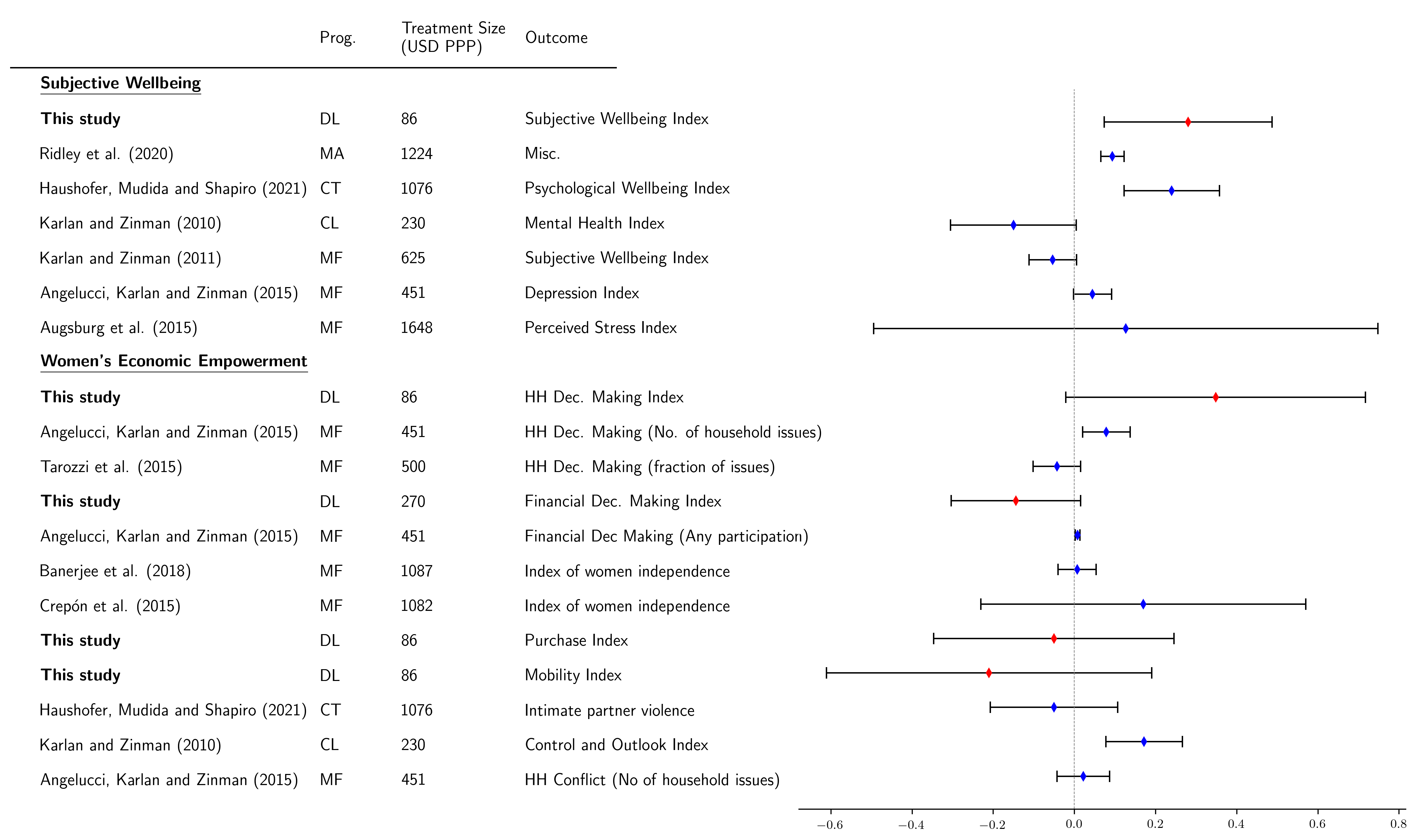
Figure A9: Effect Size Comparisons: Wellbeing, and Women’s Economic Empowerment

Our results are similar to studies which mostly find no or limited impacts of microcredit on women’s empowerment, as summarized in Appendix Figure A9. The most straightforward comparison is to studies which report summary indices (i.e., Banerjee et al., 2015; Crépon et al., 2015; Karlan and Zinman, 2011): in all cases, we observe that our confidence intervals overlap.

4.3 Subjective well-being

Perhaps our most notable finding is that access to digital credit increases subjective well-being substantially, by 0.281 standard deviations (first row of Table 2, column 5). In contrast, the amount that a borrower is allowed to access (row labeled ‘Initial Offer’) has a very small and statistically insignificant effect on subjective well-being. We measure subjective well-being with a summary index that places equal weight on self-reported life satisfaction and a standardized measure of depression, i.e., the nine questions from the Patient Health Questionnaire-9 (PHQ-9). As can be seen in Panel A of Figure 1, the positive effect of loan access on subjective well-being is driven by the PHQ-9 score. Applicants allowed to borrow report being less depressed and report feeling less likely to suffer from poor appetite or overeating. We find small effects on other a number of other components of the PHQ-9, though most of these are only significant at the 10% level after multiple hypothesis testing adjustments.

4.4 Discussion

The improvements in subjective well-being we find are large, even relative to those of intensive antipoverty interventions (Appendix Figure A9). For instance, the meta-analysis by Ridley et al. (2020) finds that multifaceted antipoverty programs increase well-being by 0.17 standard deviations, and cash transfer programs on average increase mental health by 0.105 standard deviations; Angelucci et al. (2015) finds that access to microfinance reduces a depression index by 0.045 standard deviations. Relative to these studies, the effect we observe of 0.281 standard deviations are quite large.Perhaps most striking is the fact that these other programs involve much larger transfers: in Ridley et al. (2020), the average multifaceted antipoverty program cost $1,707 PPP and the average cash transfer was $956 PPP; and the average loan value in Angelucci et al. (2015) was $840 PPP. In our experiment, respondents borrowed an additional $30 ($86 PPP) when assigned to auto-approval — though some still owed money to the FSP at the time of the survey (46% of the credit that applicants received had yet to be repaid at the time of the survey). We therefore speculate briefly on the mechanisms that might be driving these substantial effects.

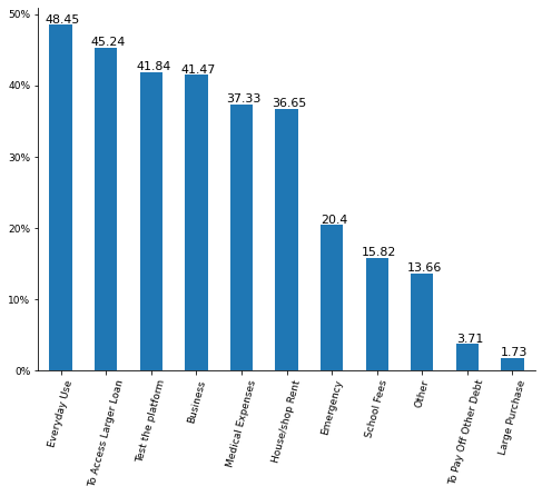
Figure A11: Loan Purpose

For context, we observe that short-run needs are the most common reasons that our sample reports taking a loan (Figure A11). These needs include everyday use (49%), business purposes (42%), medical expenses (37%), paying house/shop rent (37%) and emergencies (20%). While the loans are small, such uses could reduce the depressive symptoms observed in Figure 1. This may be especially true in the Nigerian context, where rates of depression and mental disorder are quite high.

There is also suggestive evidence that the effects on subjective well-being are larger for certain types of individuals. Table 3 disaggregates the well-being effects by several key sources of heterogeneity in our population. Broadly, we observe that people with lower credit scores and those who are unemployed tend to have lower subjective well-being (rows 8-9), and that access to digital credit improves subjective well-being more for these two groups (rows 2-3). In fact, when individuals of both types are auto-approved, this differential effect is sufficient to close the gap in subjective well-being between unemployed and employed, and more than closes the gap by credit score (row 3 vs. row 9, and row 2 vs. row 8). We also find larger impacts on applicants who own a business (row 4), but little difference in impact by gender (row 5). These findings hold also when the effect is allowed to vary by all of these characteristics simultaneously (column 5). However, this heterogeneity analysis should be viewed speculatively, as it was not a part of our pre-registration plan, and the heterogeneous impact estimates are generally not statistically significant.

More broadly, when trying to understand why increasing access to small loans should have comparable effects on subjective well-being as cash transfer programs, it is important to consider when and to whom benefits are provided. Our experiment considers applicants who requested immediate access to small amounts of credit, and compares those who randomly received loans to those who did not. There has been remarkable demand for this form of product across the developing world. In contrast, cash transfer programs often allocate broadly, at times determined by the program.

The comparison to microcredit is more nuanced. Microcredit typically provides larger loans but has an involved application and repayment process so may be less suited to immediate needs. Other evidence suggests that access to microcredit can reduce symptoms of depression; for instance, Fernald et al. (2008) find that increased access to microcredit decreased depressive symptoms from 15% to 2% for men (but had no significant effect for women). However, it was accompanied by increased stress. Field et al. (2012) finds that the design of the microcredit loans can contribute to stress: changing the repayment schedule to monthly rather than weekly resulted in borrowers being 51 percent less likely to report feeling ‘worried, tense, or anxious’ about repaying. Part of the improvements in subjective well-being from digital loans may arise from the security of anticipating that one can borrow in the future as needs arise. Borrowers in our sample anticipate future borrowing, and may view digital loans similarly to a line of credit.

That we find large effects for extensions of credit that are much smaller than other interventions — and that we find no effect of providing larger loan offers — suggests that even small relaxations of credit constraints delivered in moments of need may alleviate some mental health burdens. Overall, these results are consistent with a growing body of evidence supporting the notion that being unable to access small but critical resources in times of need may be quite damaging for mental health (Haushofer and Fehr, 2014; Banerjee et al., 2020).

5 Conclusion

The dramatic uptake of digital loans across the developing world suggests a pent-up demand for consumer credit. However, the structure of the digital loan market – which offers new borrowers short-term loans at high interest rates, and results in high rates of default – has led to widespread public concern over the potential consequences of this financial transformation.

Our randomized controlled trial finds that increasing access to digital loans can improve subjective well-being among applicants, measured after an average of three months. The magnitude of this effect is similar to that of costly anti-poverty interventions, even though the digital loans we study do not consume government or donor resources. This result highlights how even small relaxations of constraints can substantially improve mental health. At the same time, we do not find that offering applicants larger loans has any significant effect. We can also rule out large positive – and negative – effects of digital credit access on other dimensions of welfare, including income and expenditures, resilience, and women’s economic empowerment.

Tables and Figures

Table 1: Impacts of Digital Credit Access on Borrowing and Finances

[H] (1) (2) (3) (4) (5) (6) (7) (8) (9) Borrowing Finances Total Borrowing from FSP Any Loan Any Non-FSP Loan Formal Borrowing Index Informal Borrowing Index Loans Taken Out / Total Income Income Expenditure Total Saving (NGN) (p.p.) (p.p.) (SD) (SD) (Category) (Asinh) (Asinh) Auto-Approval *Under-threshold 11656.6 0.368 -0.033 0.877 -0.326 0.079 -0.138 0.005 -0.754 (1797.0)*** (0.051)*** (0.061) (0.096)*** (0.094)*** (0.014)*** (0.245) (0.254) (0.730) Auto-Approval *Over-threshold 1226.8 0.009 -0.007 0.112 -0.040 -0.010 0.167 0.106 -0.426 (1476.6) (0.018) (0.030) (0.051)** (0.042) (0.011) (0.111) (0.106) (0.362) Initial Offer 1239.0 -0.001 -0.003 -0.008 0.004 0.005 0.008 -0.013 -0.008 (136.3)*** (0.002) (0.003) (0.005)* (0.004) (0.001)*** (0.011) (0.010) (0.034) Mean dep var. (Standard approval group) 20036.676 0.832 0.450 -0.005 0.001 0.098 2.301 8.929 5.632 N 1611 1611 1611 1611 1611 1553 1553 1437 1440

• Notes: Each column is a separate regression. Each regression controls for respondent gender, education, head of the household, ethnicity, location (state), household size, age and respondent’s credit score status (1=under threshold) at the time of enrolment. We include enumerator, and week of enrolment fixed effects. 29 respondents did not report their age – we code these values as 0, and include a dummy variable that controls for these missing values. The index variables in columns (4) and (5) include data on the number, and amount of loans from formal and informal sources respectively. In Columns (6) and (7), monthly income is an ordinal variable, defined using the following brackets: 0 - 9,999 NGN, 10,000 - 49,999 NGN, 50,000 - 99,999 NGN, 100,000 - 249,999 NGN and $>$ 250,000 NGN. The outcome variable in Column (6) is the ratio of self-reported borrowing (over 3 months, in NGN) and self-reported income (over 3 months – we use the midpoint of each respondents monthly income brackets, and multiply by 3). Further details on how each outcome variable is constructed are provided in Appendix A1.3. The coefficients in Column (7) are from an ordinal logit regression. Parentheses contain robust standard errors.

Table 2: Impacts of Digital Credit Access on Pre-Specified Measures of Welfare

[H] (1) (2) (3) (4) (5) Resilience Fin. Health Resilience Fin. Resilience WEE Subj. Well- Index Index Index Index Being Index (SD) (SD) (SD) (SD) Auto-Approval *Under-threshold 0.024 0.014 -0.069 -0.093 0.281 (0.018) (0.080) (0.096) (0.076) (0.106)*** [0.166] [0.860] [0.718] [0.226] [0.008] Auto-Approval *Over-threshold 0.005 0.048 0.014 0.062 -0.013 (0.008) (0.034) (0.046) (0.033)* (0.049) [0.565] [0.286] [0.769] [0.057] [0.796] Initial Offer 0.001 -0.000 0.002 -0.001 0.007 (0.001)* (0.003) (0.004) (0.003) (0.004) [0.098] [0.947] [0.868] [0.678] [0.113] Mean dep var. (Standard approval group) 0.704 0.000 0.002 -0.000 -0.002 $N$ 1611 1312 1403 1611 1611

• Notes: Each column is a separate regression. Details on how each index is constructed are provided in Appendix A1.3. In brief: (1) includes 14 standardized questions about financial health; (2) includes 7 questions about coping with negative shocks (conditional on having experienced a negative shock); (3) includes two questions about the respondent’s ability to access resources in the event of a shock; (4) is an index of Women’s Economic Empowerment (WEE) that includes data on female decision-making, purchases and mobility and beliefs about female autonomy; (5) includes a measure of self-reported life satisfaction, and a standardized measure of depression. Each regression controls for respondent gender, education, head of the household, ethnicity, location (state), household size, age, and respondent’s credit score status (1 = under threshold) at the time of enrolment. We include enumerator, and week of enrolment fixed effects. 29 respondents did not report their age – we code these values as 0, and include a dummy variable that controls for these missing values. Parentheses contain robust standard errors, and square brackets contain p-values. For resilience outcomes, we report p-values after adjusting for multiple hypothesis testing, using the Sidak-Holm adjustment.

Table 3: Treatment Effect Heterogeneity: Subjective Well-being

[H] (1) (2) (3) (4) (5) Auto-approval * Under-threshold 0.436 0.230 0.236 0.284 0.219 (0.163)*** (0.132)* (0.152) (0.212) (0.312) Auto-approval * Under-threshold * Credit Score -2.316 -2.107 (2.126) (2.136) Auto-approval * Under-threshold * Unemployed 0.167 0.259 (0.222) (0.261) Auto-approval * Under-threshold * Business 0.123 0.220 (0.213) (0.248) Auto-approval * Under-threshold * Male 0.010 0.031 (0.244) (0.241) Auto-approval * Over-threshold -0.014 -0.012 -0.014 -0.014 -0.012 (0.049) (0.049) (0.049) (0.049) (0.049) Initial Offer 0.007 0.007 0.007 0.007 0.006 (0.004) (0.004) (0.004) (0.004) (0.004) Credit Score 0.280 0.271 0.283 0.282 0.262 (0.112)** (0.112)** (0.112)** (0.112)** (0.112)** Unemployed -0.129 -0.179 -0.130 -0.128 -0.182 (0.070)* (0.081)** (0.072)* (0.071)* (0.081)** Business 0.123 0.125 0.120 0.123 0.108 (0.046)*** (0.046)*** (0.049)** (0.046)*** (0.049)** Male -0.121 -0.120 -0.121 -0.141 -0.143 (0.060)** (0.060)** (0.060)** (0.066)** (0.066)** Mean dep var. (Standard approval group) -0.00 -0.00 -0.00 -0.00 -0.00 N 1611 1611 1611 1611 1611

• Each column is a separate regression, where we examine heterogeneity in treatment effects. The credit score ranges from 0-1. Business, Male and Unemployed are binary variables. Note that in the regressions in columns (1)-(4), we also include the under-threshold dummy, and an interaction with the under-threshold dummy and the characteristic of interest. In column (5), we include the under-threshold dummy, and interactions of the under-threshold dummy with all heterogeneity characteristics. These coefficients are not displayed in this table. Parentheses contain robust standard errors.

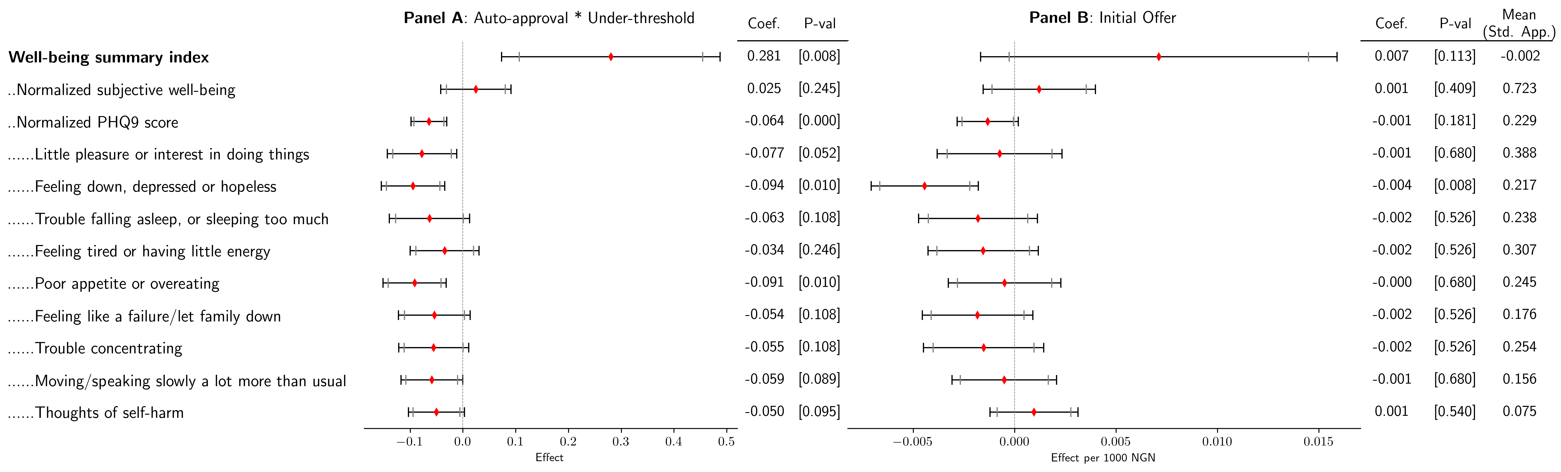
Figure 1: Subjective Well-being

Notes: This figure presents reduced form results for measures of subjective well-being. The regression specification is described in Section 3.2. Black whiskers represent 95% confidence intervals, and grey whiskers represent 90% confidence intervals. In each regression, we control for respondent gender, education, ethnicity, location (state), household size, head of household, age, and respondent’s credit score status (1=under threshold) at the time of enrolment. We also include enumerator and week of enrolment fixed effects. Since we have only one main pre-specified outcome (the well-being summary index) for this family, we report the unadjusted p-value for this outcome. We adjust p-values for False Discovery Rate (FDR) for the normalized subjective-wellbeing question, and the normalized PHQ9-score. We also adjust p-values for FDR for the 9 components of the PHQ-9 scale. Note that the PHQ-9 scale can range from 0-27; for ease of visual presentation, we divide the total PHQ-9 score for each respondent by 27, so that the value ranges from 0 to 1. Lower values on the PHQ-9 scale indicate lower levels of depression. Thus negative coefficients for the normalized PHQ-9 score and its components represent improvements in depression.

Appendix A1 Appendix

Notes: This figure presents the mean amount of each loan ($n$th loan, conditional on having borrowed the $(n-1)$th loan), as customers progress up the loan ladder, using loan data provided by the partner FSP for our sample of 1618 customers. For example, the first bar is the mean size of the first loan taken out; roughly 80% of our sample takes out at least one loan, so the mean is calculated over this set of customers. The second bar is the mean size of the second loan taken out; roughly 70% of customers take out a second loan, and we use this set of customers to calculate the mean. Black lines indicate 95% confidence intervals.

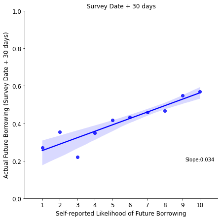
Figure A2: Likelihood of Future Borrowing

Notes: The outcome variable is based on the following survey question: “What is the likelihood that you will try to take out another loan from FSP in the next month on a scale from 1 to 10 where 1 is definitely not and 10 is certainly?” We subtract 1 and divide by 9, so that the value ranges between 0 and 1.

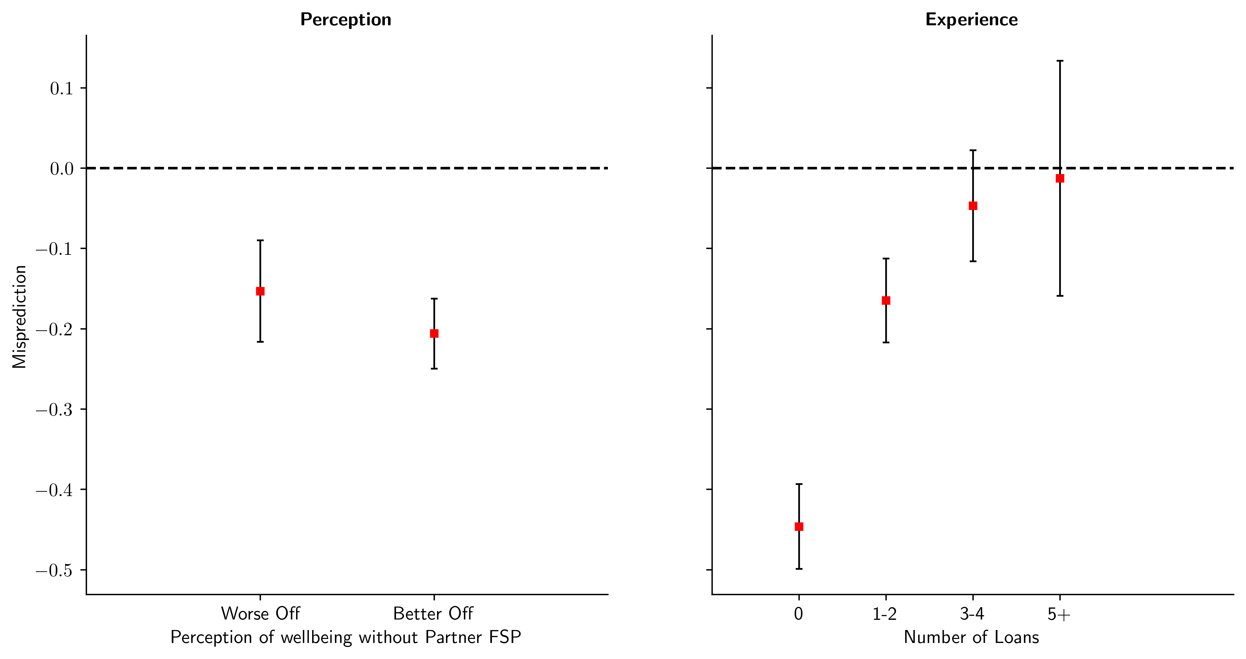
Figure A3: Misprediction of Future Borrowing

Notes:Misprediction (y-axis) is defined as the actual borrowing probability (based on administrative data 1 month after the survey) minus the predicted likelihood of borrowing in the next month (as defined in Figure A2). Perception of wellbeing without partner FSP is self-reported. Number of loans is the total number of loans borrowed from the partner FSP in the 3 months prior to survey. This figure only includes the standard approval group.

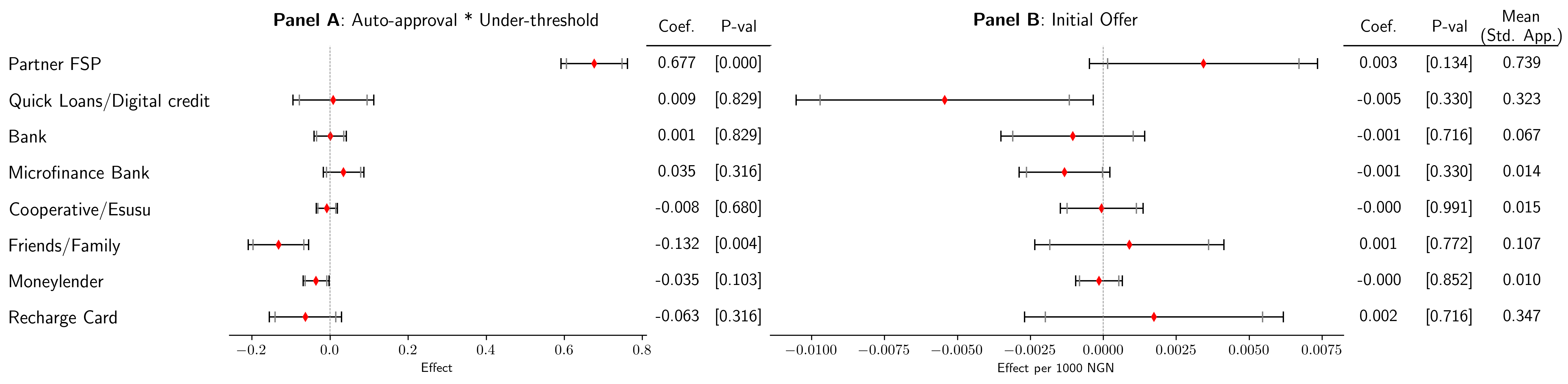
Figure A5: Self-reported Loan Sources

Notes: This figure presents reduced form results for self reported borrowing. Each outcome is a dummy variable indicating whether the respondent has borrowed at least once from that source, in the 3 months preceding the survey. The regression specification is described in Section 3.2. In each regression, we control for respondent gender, education, ethnicity, location (state), household size, head of household, age, and respondent’s credit score status (1=under threshold) at the time of enrolment. We also include enumerator and week of enrolment fixed effects. Black whiskers represent 95% confidence intervals, and grey whiskers represent 90% confidence intervals.

Figure A6: Financial Outcomes

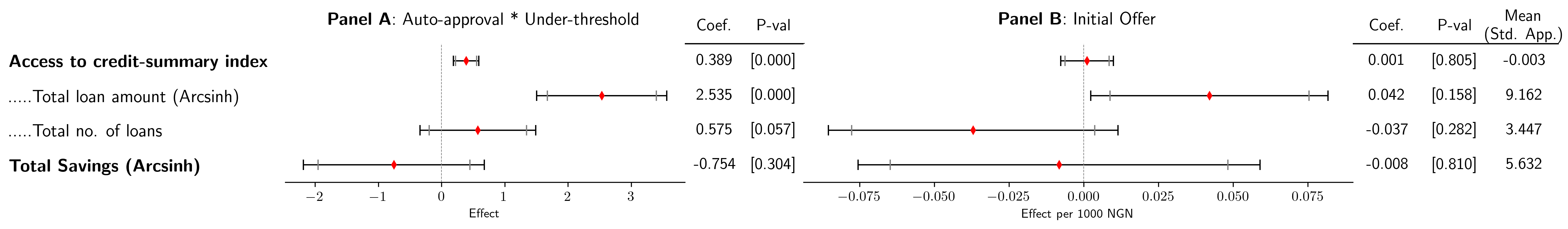
(a) Use of credit, and Savings

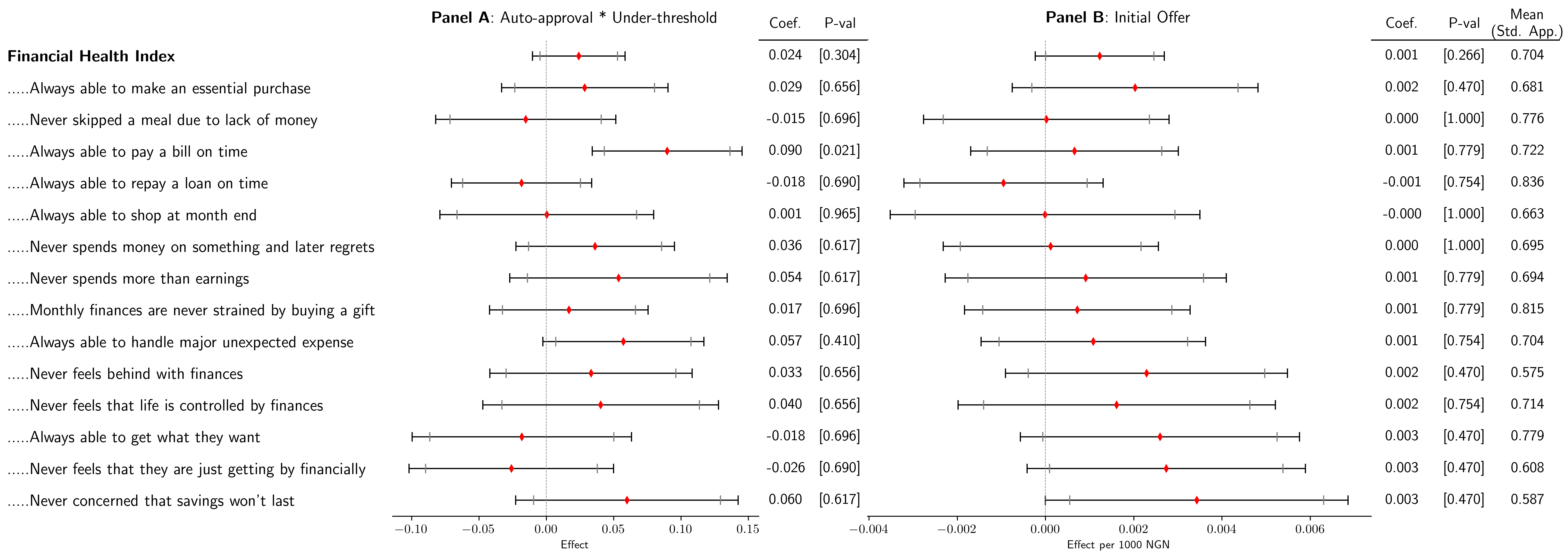
(b) Financial Health

Notes: This figure presents reduced form results for formal and informal borrowing, and savings outcomes (Row 1), and the financial health score and its sub-components (Row 2). The financial health score aggregates responses from 14 questions that capture various dimensions of the financial health. The financial health score is normalized to range between 0 and 1. The regression specification is described in Section 3.2. In each regression, we control for respondent gender, education, ethnicity, location (state), household size, head of household, age, and respondent’s credit score status (1=under threshold) at the time of enrolment. We also include enumerator and week of enrolment fixed effects. Black whiskers represent 95% confidence intervals, and grey whiskers represent 90% confidence intervals. P-values are adjusted for Family Wise Error Rate (FWER) for the main outcomes (bold) and for False Discovery Rate (FDR) for components/ sub-components (indented).

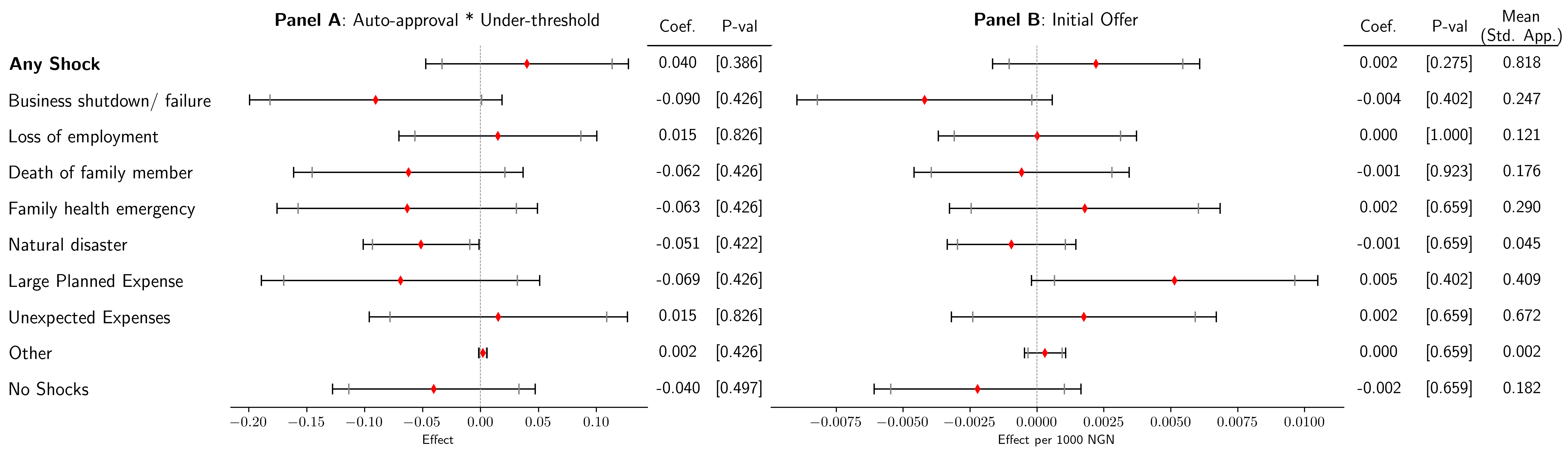
Figure A7: Shocks Experienced

Notes: This figure presents reduced form results for shocks experienced by the respondent’s household in the last 3 months. In bold, we present the coefficients from a dummy variable =1 if the respondent has experienced any of the shocks below it, and 0 otherwise. The regression specification is described in Section 3.2. In each regression, we control for respondent gender, education, ethnicity, location (state), household size, head of household, age, and respondent’s credit score status (1=under threshold) at the time of enrolment. We also include enumerator and week of enrolment fixed effects. Black whiskers represent 95% confidence intervals, and grey whiskers represent 90% confidence intervals. All p-values are FDR adjusted. Note that negative coefficients indicate that a respondent is less likely to have experienced a given shock in the last 3 months.

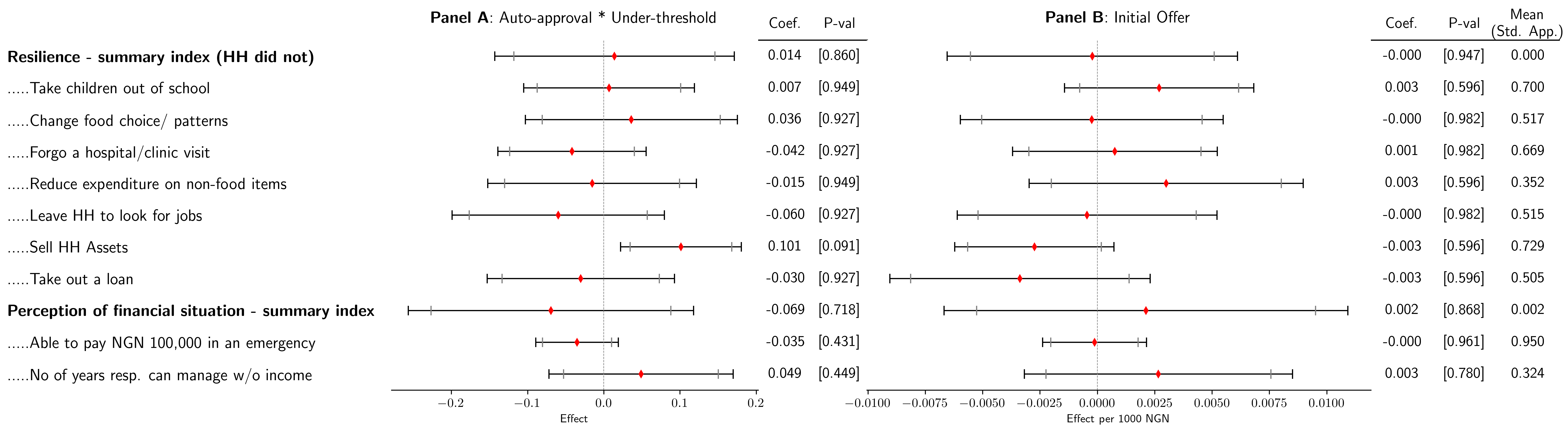
Figure A8: Resilience

This figure presents reduced form results for resilience outcomes. The regression specification is described in Section 3.2. In each regression, we control for respondent gender, education, ethnicity, location (state), household size, head of household, age, and and respondent’s credit score status (1=under threshold) at the time of enrolment. We also include enumerator and week of enrolment fixed effects. Black whiskers represent 95% confidence intervals, and grey whiskers represent 90% confidence intervals. P-values are adjusted for Family Wise Error Rate (FWER) for the main outcomes (bold) and for False Discovery Rate (FDR) for components/ sub-components (indented).

Notes: This figure plots estimated treatment effects on expenditure from evaluations of digital credit products and various anti-poverty programs. We report coefficients for the auto-approval X under-threshold group from this study in red. Column 2 indicates the type of program: DL refers to Digital Loans, CT refers to Cash Transfers, CL refers to Consumer Loans, MF refers to Microfinance, and MA refers to Meta-analysis. Column 3 is the size of the treatment in USD PPP. For this study, we report the average borrowing from the partner FSP in the last 3 months. Unless specified otherwise, treatment effects are in standard deviations, and positive coefficients indicate positive outcomes. In Ridley et al. (2020), the outcomes considered in their meta-analysis of results include instruments to detect mental illnesses and symptoms of depression, indices of psychological well-being, and a perceived stress scale.

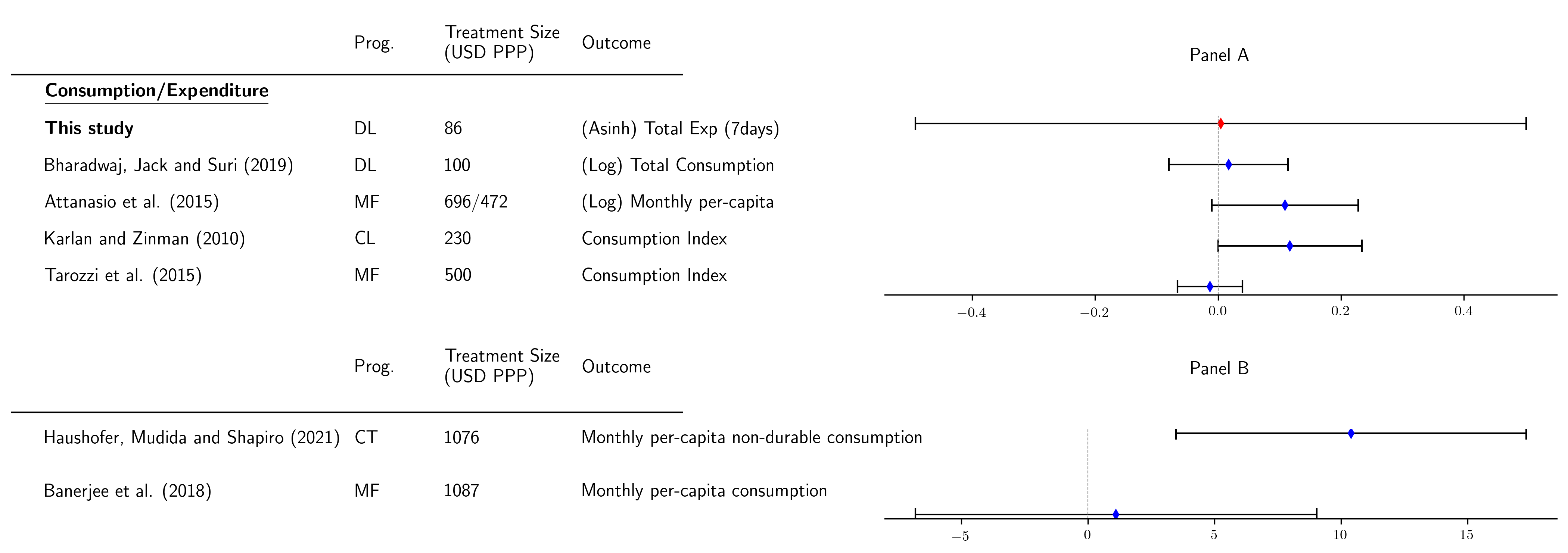
Figure A10: Effect Size Comparisons - Consumption/Expenditure

Notes: This figure plots estimated treatment effects on expenditure from evaluations of digital credit products and various anti-poverty programs. We report coefficients for the auto-approval X under-threshold group from this study in red. Column 2 indicates the type of program: DL refers to Digital Loans, CT refers to Cash Transfers, CL refers to Consumer Loans, and MF refers to Microfinance. Column 3 is the size of the treatment in USD PPP. For this study, we report the average borrowing from the partner FSP in the last 3 months. Treatment effects are in standard deviations, and positive coefficients indicate positive outcomes. In Panel B, coefficients are in USD PPP.

Notes: Each bar represents the fraction of customers in our sample that report taking out a loan at least once, for that particular purpose, across all loan sources. The exact survey question was: “For what purpose have you used the money from SOURCE (enumerator, check all that apply, do not read out) [allow multiple selections].”; respondents were asked this question for each type of loan they reported having taken out.

Table A1: Treatment Assignment – Survey Sample

[H] Initial Offer (NGN) Standard Approval Auto-Approval 1000 0.18 0.17 2000 0.20 0.16 5000 0.20 0.22 10000 0.21 0.21 13000 0.22 0.24 N 984 634

• Proportions are expressed in terms of the column totals.

Table A2: Summary Statistics - I

[H] (1) (2) Mean Weighted Mean Panel A: Demographics Age 29.936 (8.532) 29.307 (8.384) Male 0.758 (0.429) 0.760 (0.427) Location: Lagos 0.333 (0.471) 0.335 (0.472) Education: Primary 0.007 (0.082) 0.007 (0.082) Secondary 0.349 (0.477) 0.348 (0.476) HND 0.093 (0.290) 0.094 (0.292) OND 0.149 (0.356) 0.149 (0.356) University 0.357 (0.479) 0.357 (0.479) Head of household 0.447 (0.497) 0.448 (0.497) Household size 5.303 (3.199) 5.246 (3.173) Ethnicity: Yoruba 0.502 (0.500) 0.500 (0.500) Igbo 0.179 (0.383) 0.179 (0.383) Hausa 0.043 (0.202) 0.043 (0.204) Panel B: Employment/ Misc. Primary phone user 0.991 (0.093) 0.992 (0.089) Uses a bank account 0.997 (0.056) 0.997 (0.054) Employment: Self-employed 0.409 (0.492) 0.401 (0.490) Salaried (Full-time) 0.269 (0.443) 0.271 (0.445) Salaried (Part-time) 0.121 (0.326) 0.125 (0.331) Unemployed 0.201 (0.401) 0.202 (0.402) Days worked last week 3.861 (2.418) 3.871 (2.426) Runs a business 0.551 (0.498) 0.543 (0.498) Aspires to open business 0.806 (0.396) 0.790 (0.395)

• Notes: for each variable, column (1) presents the mean and standard deviation. Column (2) presents the weighted mean and standard deviation. The Ordinary National Diploma (OND) is obtained after completing a two-year course at a polytechnic. The Higher National Diploma (HND) requires an additional year of industrial training, or two years of additional coursework.

Table A3: Summary Statistics - II

[H] (1) (2) Mean Weighted Mean Panel A: Self Reported Borrowed from partner FSP 0.797 (0.402) 0.789 (0.405) No. of loans 1.869 (1.474) 1.830 (1.467) Total loan amount (NGN) 17377.760 (27522.365) 16419.976 (26317.116) Family member borrowed from Partner FSP 0.155 (0.362) 0.113 (0.312) Made a late repayment 0.342 (0.474) 0.264 (0.424) Defaulted 0.087 (0.281) 0.067 (0.248) Will borrow again (1=Most Likely) 0.617 (0.332) 0.616 (0.332) Loan terms are fair 0.855 (0.352) 0.829 (0.346) Better off without partner FSP 0.681 (0.466) 0.621 (0.451) Panel B: Administrative Data No. of loans 2.426 (1.997) 2.425 (1.999) Total loan amount (NGN) 21284.920 (26707.579) 21202.774 (26680.023) No of loan application 3.868 (3.445) 3.859 (3.332) No. of rejected applications 1.443 (3.332) 1.434 (3.224) Defaulted 0.229 (0.420) 0.185 (0.381)

• Notes: for each variable, column (1) presents the mean and standard deviation. Column (2) presents the weighted mean and standard deviation. All variables in Panel A are based on survey responses. We ask about interactions with the Partner FSP for the three-month period prior to survey. “Will borrow again” is based on the following survey question: “What is the likelihood that you will try to take out another loan from FSP in the next month (30 days) on a scale from 1 to 10 where 1 is definitely not and 10 is certainly?” We subtract 1 and divide by 9, so that the value ranges between 0 and 1. All variables in Panel B are constructed from administrative data, matched to our sample of survey respondents. We use administrative for the period between enrolment, and survey.

A1.1 Multiple hypothesis testing

We adjust p-values for multiple hypothesis testing, as described below. (And as specified in our pre-analysis plan). We consider several families of outcomes (e.g., resilience, subjective well-being etc.). For each family, we pre-specified primary outcomes of interest (e.g., the resilience summary index, and financial resilience summary index), which may summarize multiple measures (e.g., multiple questions which measure the applicant’s ability to experience a negative economic shock without forgoing expenditure or adjusting behavior). If a family contains only one primary outcome, we do not adjust p-values. If a family contains more than one primary outcome, we report p-values adjusted for Family-wise Error Rate (FWER - the probability that one or more false rejections of the null hypothesis will occur), using the Sidak-Holm adjustment. This adjustment assumes that the tests are not negatively dependent. Under this assumption, for a family of m outcomes sorted in ascending order of p-values, the following comparison is sufficient to ensure that the FWER $\leq\alpha$:

$$p_{m}\leq 1-(1-\alpha)^{(1/m)}$$ (2)

Whenever we present effects on the measures within an outcome (e.g. the individual questions that comprise the resilience summary index in Fig A8), we adjust p-values for False Discovery Rate (FDR - the expected proportion of the false rejections of the null hypothesis). We use the two stage procedure described in Benjamini et al. (2006) for FDR adjustments. This procedure assumes the independence of p-values (Anderson (2008) also argues that this procedure works well in the event that p-values are positively dependent).

A1.2 Deviations from pre-analysis plan

We make the following deviations from our pre-analysis plan:

• Outcomes:

  • We report several informative borrowing outcomes in addition to those we pre-specified. We additionally report the extensive margins of taking out any loan and any non-FSP loan, an informal borrowing index created analogously to the formal borrowing index, and the ratio of loans taken out to total income.

  • We measured income in a categorical variable, because respondents struggled to give exact income amounts during piloting.

  • The resilience family contains three measures (responses to shocks, raising emergency funds, and meeting basic needs). The pre-analysis plan grouped the first two in one outcome, and the remaining in another outcome. Because the first measure is defined only for respondents who have experienced a shock, we instead leave the first measure as its own outcome (‘resilience index’) and group the second two measures into an outcome (‘financial resilience index’).

• Specifications:

  • We interact the auto-approval treatment with a dummy for whether the applicant is under or above the credit score threshold, which more precisely describes who the treatment is affecting.

  • The pre-analysis plan suggests instrumental variables (IV) specifications in addition to OLS specifications. We focus on OLS specifications because our two treatments induce different effects. Results with IV specifications are qualitatively similar.

  • We omit week-of-survey fixed effects; we instead reweight the sample to ensure that the average time between enrolment and survey is the same across auto-approval and standard approval groups.

  • In addition to the auto-approval and standard approval groups, we also gather survey data from a group of business-as-usual customers. In the pre-analysis plan, we that we would compare both treatment arms against this business-as-usual group in our analysis. However, the business-as-usual group ended up being surveyed roughly 20 days earlier (on average) than the auto-approval and credit-score approval groups. Thus we are unable to make meaningful comparisons between borrowers in the business as usual group, and those in the auto-approval and standard approval arms. As a result of this omission, we do not estimate treatment effects using the specifications outlined in PAP sections 5.3.1 B, and 5.3.2 B. We additionally form z-scores relative to the standard approval group, rather than the business as usual group.

• Extensions:

  • We attempted to ask about demand for commitment to avoid debt traps, but responses to this question made clear that this question was not understood.

  • In this paper, we do not present an analysis of heterogeneous treatment effects using machine learning methods. This part of the analysis is still ongoing, and will likely be the subject of a separate paper.

  • We have not checked the robustness of comparing our index outcomes to ones constructed using Principal Component Analysis (PCA), or using nonparametric methods.

A1.3 Variables

Below, we briefly describe the main outcome variables we use for our main analysis. For each outcome, we mention the relevant unit, and the table in which it appears in parentheses.

1. Borrowing and Financial outcomes

1. Total borrowing from FSP (NGN, Table 1 column 1): The total amount borrowed from the partner FSP between enrolment and survey.

2. Any loan (Table 1 column 2): A binary variable equalling one if the respondent self reports taking out a loan from any source, in the last three months.

3. Any non-FSP loan (Table 1 column 3): A binary variable equalling one if the respondent self reports taking out a loan from any non-FSP source in the last three months.

4. Index of formal borrowing (standard deviations, Table 1 column 4): An equally weighed average of the z-scores of the self-reported i) total number of loans and ii) total amount borrowed, in the last 3 months from formal sources (digital credit, bank, micro-finance, or cooperative). The z-scores are constructed by subtracting the mean of the standard approval group and dividing by the standard deviation of the standard approval group.

5. Index of informal borrowing (standard deviations, Table 1 column 5): An equally weighed average of the z-scores of the self-reported i) total number of loans and ii) total amount borrowed, in the last 3 months from informal sources (friends and family, moneylenders, or airtime credit). The z-scores are constructed by subtracting the mean of the standard approval group and dividing by the standard deviation of the standard approval group.

6. Ratio of loans taken out to total income (Table 1 column 6): The ratio of self-reported borrowing over the past 3 months in NGN, and self-reported income from the last month multiplied by 3 (we use the midpoint of each individuals income bucket).

7. Income (categorical, Table 1 column 7): The respondent picks their monthly income bracket from the following categories: $<$N10,000, N10,000-N49,999, N50,000-N99,999, N100,000-N250,000, and $>$N250,000.

8. Expenditure (asinh, Table 1 column 8): The inverse hyperbolic sine of the respondent’s total self-reported household expenditure in the last 7 days.

9. Total Saving (asinh, Table 1 column 9): The inverse hyperbolic sine of the self-reported total amount saved in the three months prior to the survey (Q25).

10. Financial Health Index (Table 2 column 1): This index is constructed by aggregating responses from 14 questions that capture various dimensions of the financial health of the respondents. These questions are based on the Consumer Finance Protection Bureau (2017) financial health index, which we piloted and then adjusted in Nigeria prior to our survey. Those responses to each question are collected on a scale of 0-3 (for a maximum of 42); we divide by 42, so that our index ranges between 0 and 1.

Following our pre-analysis plan, we group our outcomes into families: subjective well-being, resilience, and women’s economic empowerment. For each family, we specified the primary outcomes in our pre-analysis plan; in most cases, these are index variables following Kling et al. (2007).

2. Resilience

1. Resilience index (standard deviations, Table 2, column 2): This index is a standardized equally weighted average of the z-scores of seven questions which capture the respondent’s coping strategies, after having faced a negative shock. The z-scores are constructed by subtracting the mean of the standard approval group and dividing by the standard deviation of the standard approval group. We construct this index for only those respondents who report having faced at least one negative shock in the three months prior to survey. We elicit information on coping strategies using the following question: In response to adverse events in the last 3 months (ones just named), has your household done any of the following (Yes/No):

   • Taken children out of school/ had children sent home from school due to outstanding school fee balance?

   • Foregone meals, or changed food choice/patterns due to monetary constraints?

   • Foregone a hospital/clinic visit when a household member was sick, or been unable to pay the full amount needed for some medical treatment?

   • Reduced expenditure on non-food items?

   • Had members leave the house to look for jobs?

   • Sold household assets?

   • Taken out a loan?

   In all cases, a ‘no’ response is treated as resilience.

2. Financial resilience index (standard deviations, Table 2 column 3): This index is a standardized and equally weighted average of the z-scores of two questions, which capture the respondent’s perceptions of their own ability to cope financially with the effects of a hypothetical negative shock. The z-scores are constructed by subtracting the mean of the standard approval group and dividing by the standard deviation of the standard approval group. The two questions used for this index are:

   • If you had one week to pay 100,000 NGN for an emergency expense, such as a repair or medical bill, who would you turn to, to get the money (read all out, check all that apply)?

   • God forbid, if your household stopped getting income from any source, how long could your household easily continue to meet your basic needs for food and housing? (Enter duration in days)

3. Women’s Economic Empowerment

We have four main outcomes that capture various dimensions of women’s economic empowerment. These index variables are based on those used in Field et al. (2019), with a few adjustments made to suit our study context. In all cases, the aim is to measure changes in economic empowerment for an adult female in the respondent’s household. If the respondent is male, we thus elicit details about their spouse/ live-in partner. Since 76% of our sample is male, this is the most common scenario. If the respondent is female, we elicit details about their own perceptions and experiences along the dimensions discussed below. Unless mentioned otherwise below, all questions in this section were administered to only those respondents who report being married or in a live-in relationship.

1. Decision-making index (standard deviations, Appendix Table A5, column 5): This is an equally weighted standardized index of z-scores constructed from two questions which measure the female’s ability to take decisions on how they spend their earnings, and whether they might seek employment outside the household. The z-scores are constructed by subtracting the mean of the standard approval group and dividing by the standard deviation of the standard approval group. The question is: “Who is responsible for making the following decisions in your household?” For each option listed below, possible answers include “you exclusively”, “mostly you” (coded as one if the respondent is female), “both you and your spouse/partner evenly” (coded as one for both females and males), “mostly your spouse/partner”, “exclusively your spouse/partner” (coded as one if the respondent is male), or “not applicable”. This variable is missing if the respondent refused to answer, or selectes “not applicable”

   • how you spend your (worded as “your spouse/partner spends her”, if the respondent is male) own earnings (meaning income you yourself earn/money you receive (“she earns/money she receives”, if the respondent is male) for benefits)?

   • whether you take (“your spouse/partner takes”, if the respondent is male) employment outside the household?

2. Purchase Index (standard deviations, Appendix Table A5, column 6): This is an equally weighted standardized index of z-scores constructed from six questions, which measure the female’s ability to make decisions on the purchase of clothing, children’s healthcare, home improvement, festivals, and meals. The z-scores are constructed by subtracting the mean of the standard approval group and dividing by the standard deviation of the standard approval group. The main question is: “Who is responsible for making the following decisions in your household?” For each option listed below, possible answers include “you exclusively”, “mostly you” (coded as one if the respondent is female), “both you and your spouse/partner evenly” (coded as one for both females and males), “mostly your spouse/partner”, “exclusively your spouse/partner” (coded as one if the respondent is male), or “not applicable”. This variable is missing if the respondent refused to answer, or selects “not applicable”

   • how much your household spends on clothing,

   • how much your household spends on your children’s health,

   • how much your household spends on home improvement,

   • how much your household spends on festivals and celebrations

   • how much your household spends on food and drink outside the home

   We also include responses from the following question “When making these purchases do you (“does your spouse/partner” if the respondent is male) usually use money provided by another household member? (Yes/No)”

3. Mobility Index (standard deviations, Appendix Table A5, column 7): This is an equally weighted standardized index constructed from the z-scores of three questions, which measure the female’s ability to visit the following locations: a market outside their neighborhood/ village, a relative’s house outside their neighborhood/ village, and a friend’s house for a social visit. For the raw values of each question, lower values indicate a higher frequency of visit/better mobility. The z-scores are constructed by subtracting the mean of the standard approval group and dividing by the standard deviation of the standard approval group. The question is: “For each location, please tell me approximately how long ago you (your spouse/partner) last visited that location, in days”. The variable is missing if the respondent refused to answer. Note that we administer these questions to all female respondents, irrespective of their relationship status.

   • Market outside neighbourhood/ village

   • Relative’s house outside neighbourhood/ village

   • A friend’s house for a social visit

4. Financial Index (standard deviations, Appendix Table A5, column 8): This is an equally weighted standardized index constructed from the z-scores of four questions, which measure beliefs about whether a female should be able to make the following financial decisions on her own: visiting a bank alone, opening a separate bank account, using their bank account without their partner/husband’s permission, and taking out a loan. Note that we administer these questions to all respondents irrespective of their relationship status. The z-scores are constructed by subtracting the mean of the standard approval group and dividing by the standard deviation of the standard approval group. The questions are: Women should be able to make their own decision to do the following (without needing the permission of their spouse/ live-in partner) [1-Completely disagree, 5-Strongly Agree]

   • Visit the bank alone

   • Open a separate bank account for themselves

   • Use bank accounts without taking permission from their spouses

   • Take out a loan

We aggregate these four indices to create a single WEE Index (standard deviations, Table 2, column 4): The equally weighted average of the decision-making, purchase, mobility and financial indices. For this variable, we ignore missing values in any of these component indices.

4. Subjective well-being

1. Index of subjective well-being (standard deviations, Table 2 column 5, Table 3, and Figure 1): The subjective well-being index is a standardized and equally weighted average of two variables: the respondents’ z-score on the PHQ-9 questionnaire, and the z-score of their response to a life satisfaction question, similar to those in the World Values Survey. Note that the respondent’s PHQ-9 score can range from 0-27; for ease of visual presentation, we divide the total PHQ-9 score by 27, so that the value ranges from 0 to 1. A lower PHQ-9 score indicates lower levels of depression. The z-scores are constructed by subtracting the mean of the standard approval group and dividing by the standard deviation of the standard approval group. The life satisfaction question we use is: All things considered, how satisfied are you with your life as a whole these days? (Very happy/ quite happy/ not very happy/ not at all happy)

References

- (1)
- Ahn et al. (2018) Ahn, Michael, Mike Batty, and Ralf R. Meisenzahl, “Household Debt-to-Income Ratios in the Enhanced Financial Accounts,” January 2018.
- Allcott et al. (2021) Allcott, Hunt, Joshua J. Kim, Dmitry Taubinsky, and Jonathan Zinman, “Are High-Interest Loans Predatory? Theory and Evidence from Payday Lending,” Working Paper 28799, National Bureau of Economic Research May 2021. Series: Working Paper Series.
- Anderson (2008) Anderson, Michael L., “Multiple Inference and Gender Differences in the Effects of Early Intervention: A Reevaluation of the Abecedarian, Perry Preschool, and Early Training Projects,” Journal of the American Statistical Association, 2008, 103 (484), 1481–1495.
- Angelucci et al. (2015) Angelucci, Manuela, Dean Karlan, and Jonathan Zinman, “Microcredit Impacts: Evidence from a Randomized Microcredit Program Placement Experiment by Compartamos Banco,” American Economic Journal: Applied Economics, January 2015, 7 (1), 151–182.
- Attanasio et al. (2015) Attanasio, Orazio, Britta Augsburg, Ralph De Haas, Emla Fitzsimons, and Heike Harmgart, “The Impacts of Microfinance: Evidence from Joint-Liability Lending in Mongolia,” American Economic Journal: Applied Economics, January 2015, 7 (1), 90–122.
- Augsburg et al. (2015) Augsburg, Britta, Ralph De Haas, Heike Harmgart, and Costas Meghir, “The Impacts of Microcredit: Evidence from Bosnia and Herzegovina,” American Economic Journal: Applied Economics, January 2015, 7 (1), 183–203.
- Banerjee et al. (2015) Banerjee, Abhijit, Esther Duflo, Rachel Glennerster, and Cynthia Kinnan, “The Miracle of Microfinance? Evidence from a Randomized Evaluation,” American Economic Journal: Applied Economics, January 2015, 7 (1), 22–53.
- Banerjee et al. (2020) , Michael Faye, Alan Krueger, Paul Niehaus, and Tavneet Suri, “Effects of a Universal Basic Income during the pandemic,” UC San Diego Technical Report, 2020.
- Benjamini et al. (2006) Benjamini, Yoav, Abba M. Krieger, and Daniel Yekutieli, “Adaptive Linear Step-up Procedures That Control the False Discovery Rate,” Biometrika, 2006, 93 (3), 491–507.
- Bharadwaj et al. (2019) Bharadwaj, Prashant, William Jack, and Tavneet Suri, “Fintech and Household Resilience to Shocks: Evidence from Digital Loans in Kenya,” National Bureau of Economic Research Working Paper Series, February 2019.
- Bhutta et al. (2016) Bhutta, Neil, Jacob Goldin, and Tatiana Homonoff, “Consumer Borrowing after Payday Loan Bans,” The Journal of Law and Economics, February 2016, 59 (1), 225–259. Publisher: The University of Chicago Press.
- Bhutta et al. (2015) , Paige Marta Skiba, and Jeremy Tobacman, “Payday Loan Choices and Consequences,” Journal of Money, Credit and Banking, 2015, 47 (2-3), 223–260. _eprint: https://onlinelibrary.wiley.com/doi/pdf/10.1111/jmcb.12175.
- Björkegren and Grissen (2020) Björkegren, Daniel and Darrell Grissen, “Behavior Revealed in Mobile Phone Usage Predicts Credit Repayment,” The World Bank Economic Review, October 2020, 34 (3), 618–634.
- Brailovskaya et al. (2020) Brailovskaya, Valentina, Pascaline Dupas, and Jonathan Robinson, “Digital Credit: Filling a hole, or digging a hole? Evidence from Malawi,” Working Paper 2020.
- Carrell and Zinman (2014) Carrell, Scott and Jonathan Zinman, “In Harm’s Way? Payday Loan Access and Military Personnel Performance,” The Review of Financial Studies, September 2014, 27 (9), 2805–2840.
- Consumer Finance Protection Bureau (2017) Consumer Finance Protection Bureau, “CFPB Financial Well-Being Scale,” Technical Report, Consumer Financial Protection Bureau 2017.
- Crépon et al. (2015) Crépon, Bruno, Florencia Devoto, Esther Duflo, and William Parienté, “Estimating the Impact of Microcredit on Those Who Take It Up: Evidence from a Randomized Experiment in Morocco,” American Economic Journal: Applied Economics, January 2015, 7 (1), 123–150.
- de Mel et al. (2008) de Mel, Suresh, David McKenzie, and Christopher Woodruff, “Returns to Capital in Microenterprises: Evidence from a Field Experiment,” The Quarterly Journal of Economics, 2008, 123 (4), 1329–1372.
- de Mel et al. (2009) , , and , “Are Women More Credit Constrained? Experimental Evidence on Gender and Microenterprise Returns,” American Economic Journal: Applied Economics, July 2009, 1 (3), 1–32.
- Dhingra et al. (2011) Dhingra, Satvinder S., Matthew M. Zack, Tara W. Strine, Benjamin G. Druss, Joyce T. Berry, and Lina S. Balluz, “Psychological Distress Severity of Adults Reporting Receipt of Treatment for Mental Health Problems in the BRFSS,” Psychiatric Services, 2011, 62 (4), 396–403. PMID: 21459991.
- Donovan and Park (2019) Donovan, Kevin P. and Emma Park, “Perpetual Debt in the Silicon Savannah,” August 2019.
- EFInA (2021) EFInA, “EFInA Access to Financial Services in Nigeria, 2020,” Technical Report 2021.
- Fernald et al. (2008) Fernald, Lia CH, Rita Hamad, Dean Karlan, Emily J. Ozer, and Jonathan Zinman, “Small individual loans and mental health: a randomized controlled trial among South African adults,” BMC Public Health, 2008, 8 (1), 409.
- Field et al. (2019) Field, Erica M, Rohini Pande, Natalia Rigol, Simone G Schaner, and Charity Troyer Moore, “On Her Own Account: How Strengthening Women’s Financial Control Affects Labor Supply and Gender Norms,” Working Paper 26294, National Bureau of Economic Research September 2019.
- Field et al. (2012) Field, Erica, Rohini Pande, John Papp, and Y. Jeanette Park, “Repayment Flexibility Can Reduce Financial Stress: A Randomized Control Trial with Microfinance Clients in India,” PLOS ONE, September 2012, 7 (9), e45679. Publisher: Public Library of Science.
- Francis et al. (2017) Francis, Eilin, Joshua E. Blumenstock, and Jonathan Robinson, “Digital Credit: A Snapshot of the Current Landscape and Open Research Questions,” Working Paper 516, BREAD 2017.
- Gathergood et al. (2019) Gathergood, John, Benedict Guttman-Kenney, and Stefan Hunt, “How Do Payday Loans Affect Borrowers? Evidence from the U.K. Market,” The Review of Financial Studies, February 2019, 32 (2), 496–523.
- Haushofer and Fehr (2014) Haushofer, Johannes and Ernst Fehr, “On the psychology of poverty,” Science, May 2014. Publisher: American Association for the Advancement of Science.
- Hindenburg Research (2020) Hindenburg Research, “Opera: Phantom of the Turnaround – 70% Downside,” January 2020.
- Johnen et al. (2021) Johnen, Constantin, Martin Parlasca, and Oliver Mußhoff, “Promises and pitfalls of digital credit: Empirical evidence from Kenya,” PLOS ONE, July 2021, 16 (7), e0255215. Publisher: Public Library of Science.
- Karlan and Zinman (2010) Karlan, Dean and Jonathan Zinman, “Expanding Credit Access: Using Randomized Supply Decisions to Estimate the Impacts,” The Review of Financial Studies, 11 2010, 23 (1), 433–464.
- Karlan and Zinman (2011) and , “Microcredit in Theory and Practice: Using Randomized Credit Scoring for Impact Evaluation,” Science, June 2011, 332 (6035), 1278–1284.
- Karlan et al. (2014) , Robert Osei, Isaac Osei-Akoto, and Christopher Udry, “Agricultural Decisions after Relaxing Credit and Risk Constraints,” The Quarterly Journal of Economics, 2014, 129 (2), 597–652.
- Kling et al. (2007) Kling, Jeffrey R., Jeffrey B. Liebman, and Lawrence F. Katz, “Experimental Analysis of Neighborhood Effects,” Econometrica, 2007, 75 (1), 83–119.
- Meager (2019) Meager, Rachael, “Understanding the Average Impact of Microcredit Expansions: A Bayesian Hierarchical Analysis of Seven Randomized Experiments,” American Economic Journal: Applied Economics, 2019, 11 (1), 57–91.
- Melzer (2011) Melzer, Brian T., “The Real Costs of Credit Access: Evidence from the Payday Lending Market*,” The Quarterly Journal of Economics, February 2011, 126 (1), 517–555.
- Melzer (2018) Melzer, Brian T, “Spillovers from Costly Credit,” The Review of Financial Studies, September 2018, 31 (9), 3568–3594.
- Morgan et al. (2012) Morgan, Donald P., Michael R. Strain, and Ihab Seblani, “How Payday Credit Access Affects Overdrafts and Other Outcomes,” Journal of Money, Credit and Banking, 2012, 44 (2/3), 519–531. Publisher: Wiley.
- Morse (2011) Morse, Adair, “Payday lenders: Heroes or villains?,” Journal of Financial Economics, October 2011, 102 (1), 28–44.
- Perng et al. (2018) Perng, Julia, Kevin McGee, Gbemisola Oseni, Ryoko Sato, and Tomomi Tanaka, “Depression and its links to conflict and welfare in Nigeria,” January 2018.
- Ridley et al. (2020) Ridley, Matthew, Gautam Rao, Frank Schilbach, and Vikram Patel, “Poverty, depression, and anxiety: Causal evidence and mechanisms,” Science, 2020, 370 (6522).
- Romero et al. (2021) Romero, Jimena, Kristina Esopo, Joel McGuire, and Johannes Haushofer, “The Effect of Economic Transfers on Psychological Well-Being and Mental Health,” Working Paper 2021.
- Skiba and Tobacman (2019) Skiba, Paige Marta and Jeremy Tobacman, “Do Payday Loans Cause Bankruptcy?,” The Journal of Law and Economics, august 2019, 62 (3), 485–519.
- Suri and Jack (2016) Suri, Tavneet and William Jack, “The long-run poverty and gender impacts of mobile money,” Science, 2016, 354 (6317), 1288–1292.
- Tarozzi et al. (2015) Tarozzi, Alessandro, Jaikishan Desai, and Kristin Johnson, “The Impacts of Microcredit: Evidence from Ethiopia,” American Economic Journal: Applied Economics, January 2015, 7 (1), 54–89.
- Totolo (2018) Totolo, Edoardo, “Kenya’s Digital Credit Revolution Five Years On,” April 2018.
- Zinman (2010) Zinman, Jonathan, “Restricting consumer credit access: Household survey evidence on effects around the Oregon rate cap,” Journal of Banking & Finance, 2010, 34 (3), 546–556. Publisher: Elsevier.