Scalable Simulation and Demonstration of Jumping Piezoelectric 2-D Soft Robots

Abstract

Soft robots have drawn great interest due to their ability to take on a rich range of shapes and motions, compared to traditional rigid robots. However, the motions, and underlying statics and dynamics, pose significant challenges to forming well-generalized and robust models necessary for robot design and control. In this work, we demonstrate a five-actuator soft robot capable of complex motions and develop a scalable simulation framework that reliably predicts robot motions. The simulation framework is validated by comparing its predictions to experimental results, based on a robot constructed from piezoelectric layers bonded to a steel-foil substrate. The simulation framework exploits the physics engine PyBullet, and employs discrete rigid-link elements connected by motors to model the actuators. We perform static and AC analyses to validate a single-unit actuator cantilever setup and observe close agreement between simulation and experiments for both the cases. The analyses are extended to the five-actuator robot, where simulations accurately predict the static and AC robot motions, including shapes for applied DC voltage inputs, nearly-static "inchworm" motion, and jumping (in vertical as well as vertical and horizontal directions). These motions exhibit complex non-linear behavior, with forward robot motion reaching ~1 cm/s. Our open-source code can be found at: https://github.com/zhiwuz/sfers.

I INTRODUCTION

Soft robots have garnered interest because of their ability to take on complex shapes and motions, especially involving rich interactions with their environments. There is growing interest in leveraging the static and dynamic behavior of such robots, where for instance dynamics can enable significant speed enhancement by driving at mechanically resonant frequencies [1, 2]. This necessitates understanding the statics and dynamics through reliable models, as well as efficient integration and application of those models in simulators used for robot design and development of control systems. However, soft body modelling is challenging, due to the large number of degrees-of-freedom and complicated interactions between soft bodies and the environment (such as friction and collisions). Recent work on soft-robot modelling primarily focuses on finite-element methods [3, 4, 5, 6] and/or pseudo-rigid body models [1, 7, 8, 9, 10, 11, 12, 13].

Most recent work focuses on pneumatic soft robots [3, 4, 5, 9, 10, 12] or shape-memory and motor-tendon actuators [14, 15]. Scalable approaches for electrostatic soft robots have been more limited, with some examples including pseudo-rigid-body based modelling of a single-actuator robot [1, 7, 8, 13] and a roller made of several dielectric elastomer actuators [11, 16]. Studies on the dynamics of many-actuator piezoelectric robots have been limited.

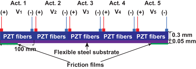
(a)

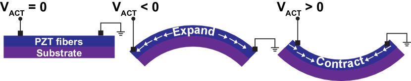
(b)

Figure 1: (a) Cross-section of the demonstrated five-actuator soft robot prototype, 500 mm long and 20 mm wide. A high friction film of 50 mm length is applied on the underside of each end. (b) Mechanism of bending, based on piezoelectric effect, whereby an actuator unit curves concave down (up) due to expansion (contraction) under negative (positive) actuator voltage.

This work addresses these challenges by developing a scalable simulation and modelling framework, generalized for a promising class of 2D soft robots, by using a motor-link model based on a pseudo-rigid body model, and experimentally validates the simulations.

We focus on a specific class of electrostatic soft robots which use piezoelectric actuators. Such soft robots allow for ease of integration and small form factors [17] as well as fast response times [1, 2]. The robot consists of a linear array of low-cost commercially-available 100-mm-long 300-µm-thick piezoelectric composites bonded to a single 50-µm-thick steel foil (side view schematics in Fig. 1(a)). Young’s modulus for the piezoelectric composites is 30 GPa, and 200 GPa of the steel foil. The demonstrated robot prototype consists of five such actuators and has a length of 500 mm and width of 20 mm. Both ends of the robot have 50-mm-long high-friction film bonded to the underside. The robot rests on a horizontal surface and is driven by external voltage sources connected by thin compliant wires.

Fig. 1(b) shows the bending mechanism of a single actuator bonded to a steel foil. When positive (negative) voltage is applied, the piezoelectric layer contracts (expands), while the bottom steel, due to its stiffness, remains nearly fixed in length. As a result, the whole structure bends concave up (down).

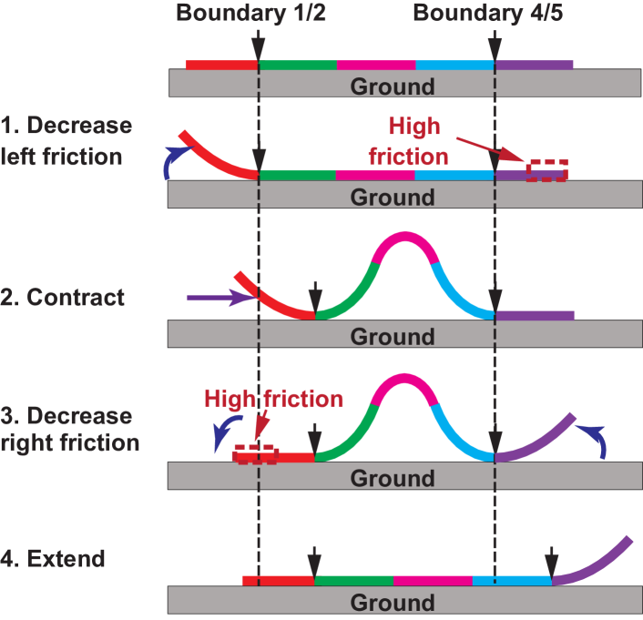
Figure 2: Inchworm motion of "contract" and "extend" cycles in 4 steps. The high-friction films at the ends are raised and lowered on opposite ends to create a friction asymmetry to generate motion. Each piezoelectric actuator in the five-actuator robot is shown in by a different color.

Fig. 2 shows a schematic view of a five-actuator robot structure used for experimental validation in this work. Inchworm-like motion is possible by exploiting asymmetry in friction alternating between its two ends: in step 1, actuator #1 (left end) is turned on to raise it to reduce friction on the left end; in step 2, actuators #2, #3, and #4 are turned on; in step 3, actuator #1 is turned off and actuator #4 is turned on, to change the end with friction; in step 4, actuators #2, #3, and #4 are turned off. The robot moves at low speed by holding a desired end fixed on the ground and then contracting/extending through its central three actuators. In addition to such motion based on robot statics, robot dynamic behaviors are also explored by operating at higher frequencies. As described later, this enables in-place and forward jumping motions.

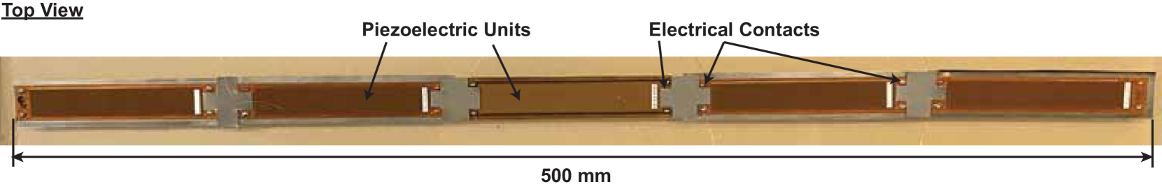
(a)

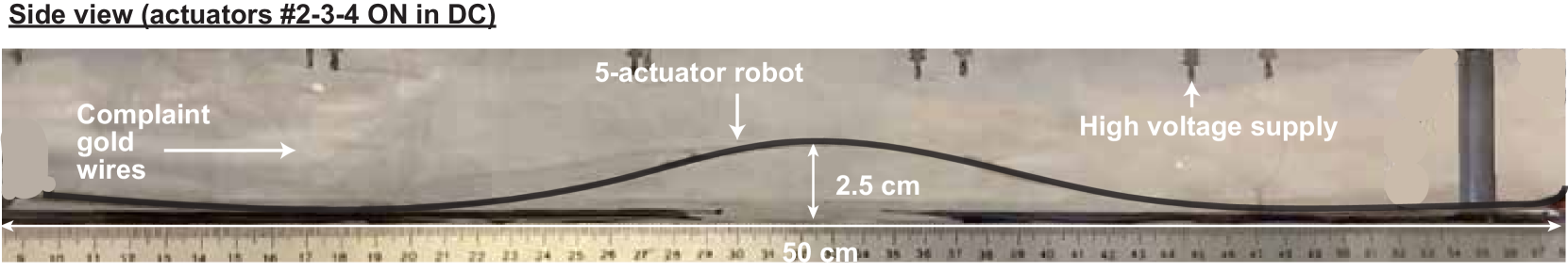
(b)

(c)

Figure 3: Robot prototype: (a) top view; (b) side view when actuated for the inchworm motion; (c) side view, when actuated for jumping motion. The five-actuator robot was placed on an acrylic pad, wired to high voltage drivers using thin and light gold wires, for real-time voltage control.

Fig. 3a shows the top view of the robot experimental setup, Fig. 3b shows the side view with actuators #2, #3, and #4 in the ON state, and Fig. 3c shows the side view, with the robot entirely off the ground in a jumping motion. Thin and light gold wires are connected from the actuator solder pads to high-voltage supplies, for robot control.

The paper has the following sections. Section II describes the PyBullet-based simulation framework and the motor-link model of a piezoelectric actuator unit in detail. Section III discusses: (1) the experimental validation of the simulation framework for the static and dynamic analyses of a single actuator; (2) the inchworm motion at low frequencies; and (3) symmetric in-place jumping of the robot, a sophisticated and inherently dynamic process which cannot be captured by close-form equation models. Section IV outlines the ongoing work related to the high-frequency behavior of the robot.

II SIMULATION FRAMEWORK

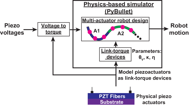
Figure 4: Simulation framework block diagram, employing motor-link actuators in PyBullet to model arrays of soft-robot actuators.

The proposed simulation framework is integrated into PyBullet (a physics-based rigid-robot simulator [18]), including effects of gravity and friction with the ground for time-domain simulations. Fig. 4 overviews the simulation framework. Piezoelectric actuators are modeled as link-torque devices within PyBullet, composing a multi-actuator robot design. To use the motor-link model, our framework converts voltages applied to the actuators into motor torques, thereby providing robot stimuli. The resulting link-torque devices then generate forces, giving rise to the robot motions. PyBullet then solves the dynamics with the discrete Newton equations (translational and rotational) for the link-torque devices.

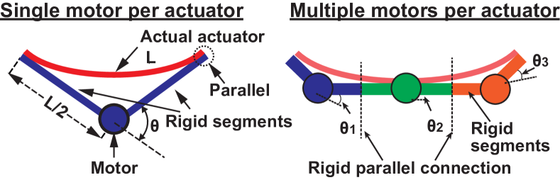
Figure 5: Modelling of an actuator: an actuator is represented by a series of motors with controlled torque connected by rigid links. Subdividing the actuator into multiple motors with shorter rigid links improves accuracy.

A key aspect of our work is the modelling of a piezoelectric actuator unit using devices comprised of two rigid links connected at a vertex at which there is a “motor” (Fig. 5). The motor applies a torque between the links. PyBullet supports such a motor, where the torque $\tau$ depends on the angle $\theta$ between the two links. To represent bending stiffness, piezoelectricity, and damping, we model the torque as proportional to: (1) the deviation of the angle from the target angle of the joint; and (2) the angular velocity:

$$\tau=-k\left(\theta-\theta_{V}+\eta\dot{\theta}\right),$$ (1)

where $k$ represents the “stiffness” of the robot; $\theta_{V}$ is a function of the voltage applied to this actuator and is determined by piezoelectricity; and $\eta$ represents the damping. A robot with multiple actuators can be modeled in PyBullet simply by connecting the end links of each actuator rigidly and in parallel to that of its neighbor. Using a boundary condition that the link ends are parallel to the piezoelectric actuator, it can be seen that multiple motors (and shorter links), with links connected rigidly in parallel, yield better shape modelling of an actuator than a single motor. Thus, we modeled each actuator parametrically, with the parameter “$m$” corresponding to the number of motor-link units (with $m=3$ by default). Critically, for dynamic modelling, the mass of the actuator is evenly subdivided into the links.

The simulation parameters $k$ and $\theta_{V}$ are deduced analytically, while $\eta$ is measured experimentally in calibration experiments employing a cantilever structure.

One can show analytically that:

$$k=\frac{EI}{2l}$$ (2)

where $EI$ is the flexural rigidity of the whole robot structure, which can be determined analytically [19], and $l$ is the link length belonging to the motor, given by

$$l=\frac{L}{2m},$$ (3)

where the factor of 2 accounts for two links connected to one motor, $L$ is the length of the actuator, and $m$ is the number of motors used to represent the actuator. Then, $\theta_{V}$ is the unloaded “target” angle of the motor:

$$\theta_{V}=\beta V/m,$$ (4)

where $V$ is the input voltage to the actuator and $\beta$ is a constant determined by piezoelectricity, given by

$$\beta =\gamma L$$ (5)

$$=\frac{d_{\text{31,1}}}{l_{\text{pitch}}}\frac{z_{1}E_{1}h_{1}}{EI}L,$$

where $\gamma$ is the bending curvature per unit voltage [19], $d_{31,1}$ is the piezoelectric constant of the piezoelectric layer, $l_{\text{pitch}}$ is the distance between the neighboring electrodes, $z_{1}$ is the position of the centerline of the piezoelectric layer w.r.t. the neutral axis, $E_{1}$ is its Young’s modulus, and $h_{1}$ is its thickness.

III EXPERIMENTAL VALIDATION

III-A Single-Actuator Cantilever

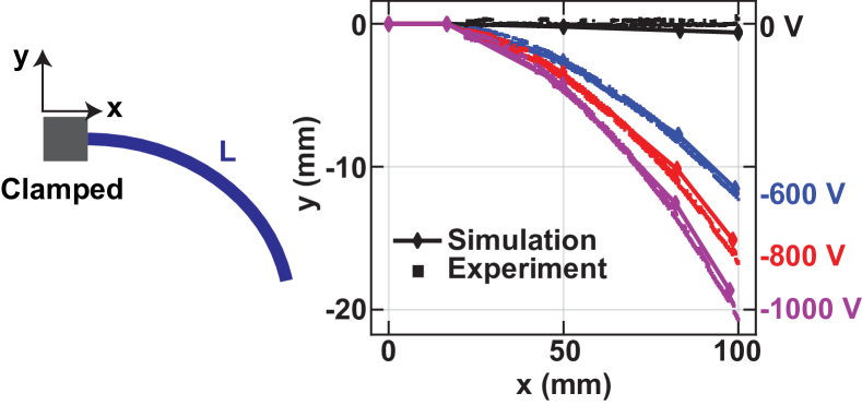
Figure 6: Experimental validation of static single-actuator cantilever simulations ($m=3$) for actuator’s static shapes, showing good agreement.

Fig. 6 shows static experimental validation of the simulation framework for an actuator in a cantilever setting. An actuator is clamped on its left end, and its right end is freely suspended. The actuator can bend up/down through different applied voltages. For instance, its free end bends down by 20 mm with -1000 V applied. Good agreement is achieved using 3-motor-link units ($m=3$).

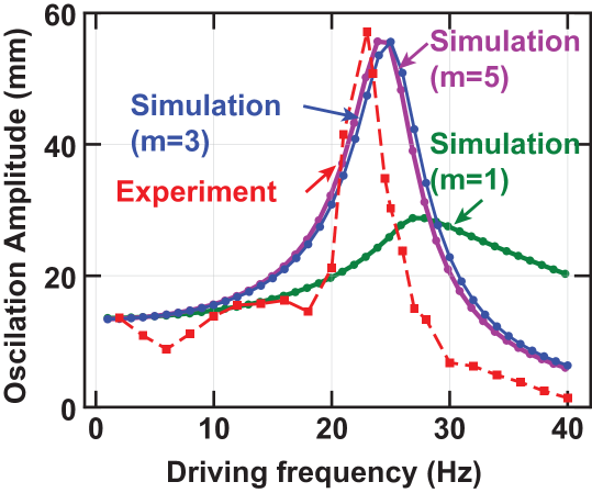
Figure 7: Experimental validation of dynamic single-actuator cantilever simulation, showing achieved oscillation amplitude vs. frequency with applied sinusoidal voltages. Note that subdividing the actuator into more motor-link units improves accuracy.

By applying a step voltage vs. time, the motor damping coefficient $\eta$ was found to be 0.03 sec. Fig. 7 validates dynamic behaviors of the cantilever, with an applied sinusoidal voltage between 0 V and -1500 V. The simulated resonant frequency (25 Hz), when $m\geq 3$, is close to the experimental 23 Hz. For the rest of the paper, $m=3$ is used as a trade-off between precision and simulation speed.

III-B Robot Static Shapes and Inchworm Motion

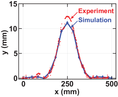
(a)

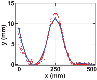
(b)

Figure 8: Experimental validation of static shape simulations of a five-actuator robot for different applied voltages: (a) $V_{1}=0$ V, $V_{2}=300$ V, $V_{3}=-960$ V, $V_{4}=300$ V, and $V_{5}=0$ V; (b) $V_{1}=300$ V, $V_{2}=300$ V, $V_{3}=-960$ V, $V_{4}=300$ V, and $V_{5}=0$ V.

Fig. 8 compares simulations and experiments for two representative robot static shapes (chosen from the inchworm motion steps of Fig. 2). Different actuators turn on or off in each case. For experimental data, the robot shapes are extracted from high-resolution images. Simulations and experiments show good agreement without any curve-fitting parameters.

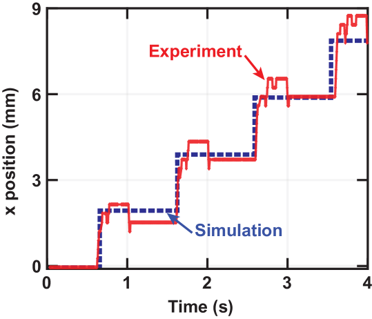
Figure 9: Experimental validation of forward inchworm-motion robot simulation.

Fig. 9 demonstrates rightward inchworm motion of the robot (as shown in Fig. 2). Different actuators turn on at different steps. The turn-on voltages are: $V_{1}=300$ V, $V_{2}=300$ V, $V_{3}=-1500$ V, $V_{4}=300$ V, and $V_{5}=300$ V. The robot moves cycle by cycle. Each cycle takes 1 s, giving overall horizontal robot motion of 1.9 mm per cycle and average speed of 1.9 mm/s. This is again in good agreement with the simulations.

III-C Robot Symmetric In-place Jumping

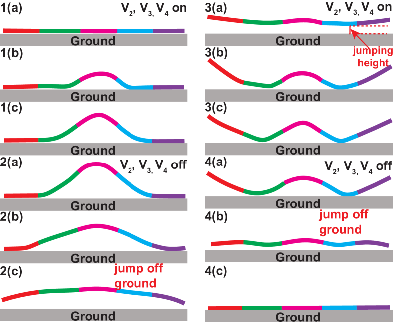
Figure 10: Robot jumping observed in experiments (from high-speed cameras) due to alternating turning $V_{2}$, $V_{3}$ and $V_{4}$ on and off. The frequency of the voltage cycling is 14 Hz. The whole robot can jump off the ground at least 7.5 mm high, referred as “jumping height” (in step 3(a)).

When the actuator driving frequency is increased, robot dynamics play a critical role. Here we examine a symmetric 2-phase jumping motion, where first the central three actuators are turned on simultaneously to lift the center section, followed by turning them off. Fig. 10 illustrates the experimentally-observed shapes (from high-speed cameras) in schematic form over two full periods. The following steps are observed beginning with an initially flat robot:

• Step 1. Actuators #2, 3 and 4 are turned on to lift the central section off the ground (as in Fig. 8(a)). Fig. 10 1(a), (b), (c) show sequential experimental shapes, indicating the generation of vertical momentum.

• Step 2. The voltages are turned off, and initially the center of mass continues to rise. With the robot becoming flatter, all parts are lifted off the ground.

• Step 3. Step 1 is repeated, but initially the robot is off the ground, so it has less time to push itself up and generate vertical momentum compared to Step 1.

• Step 4. $V_{2}$, $V_{3}$ and $V_{4}$ are turned off. With less initial vertical momentum, in Step 4 less height off the ground is obtained compared to Step 2. At the end of Step 4 the robot is flat on the ground, leading back to Step 1.

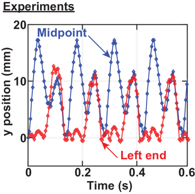
(a)

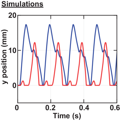
(b)

Figure 11: Time-domain movement of the robot from (a) experiments and (b) simulations, based on tracking the vertical positions of two representative points on the robot (blue line is robot midpoint, red line is robot end point). The applied voltages cycle with frequency of 14 Hz, and the frequency of periodic movement is 7 Hz. Simulations capture the doubling of the period and the phase shift between the time of maximum height for the middle vs. the ends.

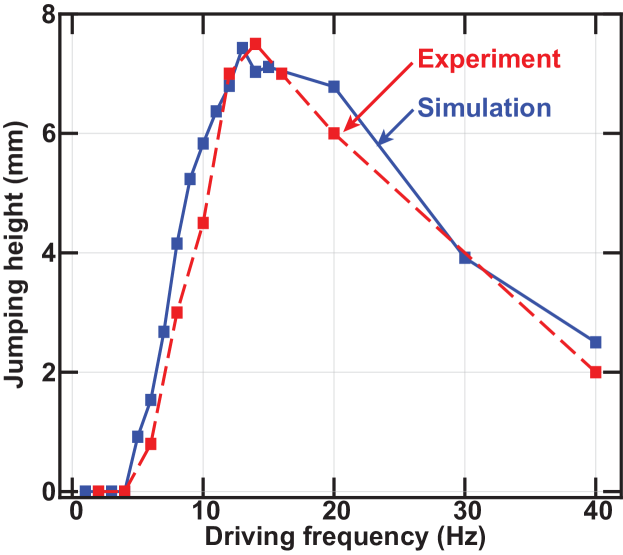
Figure 12: Jumping height vs. driving frequency using three motors per actuator (m = 3) in simulations, showing excellent agreement between simulations and experiments.

The result is a non-linear motion, with the period of maximum height being twice that of the applied voltage sequence (Fig. 11(a)). The simulation results (Fig. 11(b)) accurately capture multiple aspects of this unusual motion. Note the doubling of the motion period compared to that of the applied voltages, and the phase shift between the maximum height of the center of the robot and that of its ends. Further, Fig. 12 shows the experimental and simulated maximum height of the robot off the ground (always measured at its lowest point) during its full cycle. The robot can jump off the ground as high as ~8 mm. Remarkably good agreement between experiments and simulations is achieved without any curve-fitting parameters.

IV FAST MOTION EXPLORATION

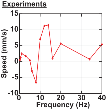
(a)

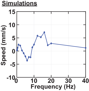
(b)

Figure 13: Robot forward speed as a function of frequency from (a) experiments and (b) simulations. Input voltage sequences are the same as the inchworm motion, but with a higher frequency. Simulation and experimental results agree qualitatively, including a reversal of direction at ~8 Hz, and maximum forward speed at ~14 Hz.

The symmetric applied voltages in the previous section lead to no left/right net motion, as expected. We now further explore frequency-dependent characteristics of the robot for the inchworm sequence of steps. The driving frequency of the control voltages is swept from low frequencies to high frequencies while maintaining the inchworm control-voltage sequencing (Fig. 13). Inchworm motion (as in Fig. 9) is observed at low frequencies (up to 3 Hz). Beyond this, a reversal in the direction of motion is observed, maximized at a frequency of 8 Hz for -7 mm/s. Further beyond this, at even higher frequencies, the robot is observed to move forward again, with a peak forward speed at 14 Hz of 12 mm/s. These frequency-dependent motions, including reversal of the movement direction, are corroborated qualitatively by the simulation, and they are currently being investigated by analyzing different vibration modes caused by different frequencies. We expect to obtain closer agreement by introducing accurately measured friction coefficients and damping factors.

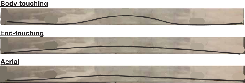
Figure 14: Three representative experimental shapes for the motion at 14 Hz driving frequency.

Fig. 14 shows three representative key shapes for the motion at 14 Hz, using the voltage waveform sequence described for the inchworm motion in Fig. 2: body-touching, end-touching, and aerial.

We now focus on understanding how such shapes and voltage-control sequences lead to “fast” forward motion. The results of this paper show that we can rely on simulation “experiments” to understand extremely complex non-linear behaviors of a soft robot, and move towards the design of optimal driving waveforms.

V CONCLUSION

The ability of soft robots to take on rich and complex motions motivates the need for a simulation framework that captures the statics and dynamics of soft robots. This work demonstrates a PyBullet-based simulation framework that models the static and dynamic behavior of planar soft robots. A motor-torque model is used to model the soft-robot actuators, and the model parameters are based on the material properties of the actuators. The static and dynamic behavior of a single-actuator cantilever setup agree closely with the experimental results. The simulator is further validated for dynamic effects such as jumping and fast forward motion at high drive frequency where dynamic effects dominate. The model will be further used to understand more complex motion and interactions with the robot’s environment.

References

- [1] Y. Wu, J. K. Yim, J. Liang, Z. Shao, M. Qi, J. Zhong, Z. Luo, X. Yan, M. Zhang, X. Wang, R. S. Fearing, R. J. Full, and L. Lin, “Insect-scale fast moving and ultrarobust soft robot,” Science Robotics, vol. 4, no. 32, p. eaax1594, jul 2019. [Online]. Available: https://robotics.sciencemag.org/lookup/doi/10.1126/scirobotics.aax1594
- [2] X. Ji, X. Liu, V. Cacucciolo, M. Imboden, Y. Civet, A. El Haitami, S. Cantin, Y. Perriard, and H. Shea, “An autonomous untethered fast soft robotic insect driven by low-voltage dielectric elastomer actuators,” Science Robotics, vol. 4, no. 37, p. eaaz6451, dec 2019. [Online]. Available: https://robotics.sciencemag.org/lookup/doi/10.1126/scirobotics.aaz6451
- [3] C. Duriez, “Control of elastic soft robots based on real-time finite element method,” in 2013 IEEE International Conference on Robotics and Automation. IEEE, may 2013, pp. 3982–3987. [Online]. Available: http://ieeexplore.ieee.org/document/6631138/
- [4] H. Zhang, Y. Wang, M. Y. Wang, J. Y. H. Fuh, and A. Senthil Kumar, “Design and analysis of soft grippers for hand rehabilitation,” ASME 2017 12th International Manufacturing Science and Engineering Conference, MSEC 2017 collocated with the JSME/ASME 2017 6th International Conference on Materials and Processing, vol. 4, pp. 1–10, 2017.
- [5] O. Goury and C. Duriez, “Fast, Generic, and Reliable Control and Simulation of Soft Robots Using Model Order Reduction,” IEEE Transactions on Robotics, vol. 34, no. 6, pp. 1565–1576, 2018.
- [6] Z. Zhang, J. Dequidt, J. Back, H. Liu, and C. Duriez, “Motion Control of Cable-Driven Continuum Catheter Robot Through Contacts,” IEEE Robotics and Automation Letters, vol. 4, no. 2, pp. 1852–1859, 2019.
- [7] N. Lobontiu, M. Goldfarb, and E. Garcia, “A piezoelectric-driven inchworm locomotion device,” Mechanism and Machine Theory, vol. 36, no. 4, pp. 425–443, apr 2001. [Online]. Available: https://linkinghub.elsevier.com/retrieve/pii/S0094114X00000562
- [8] D. Bandopadhya, “Derivation of Transfer Function of an IPMC Actuator Based on Pseudo-Rigid Body Model,” Journal of Reinforced Plastics and Composites, vol. 29, no. 3, pp. 372–390, feb 2010. [Online]. Available: http://journals.sagepub.com/doi/10.1177/0731684408097778
- [9] C. M. Best, M. T. Gillespie, P. Hyatt, L. Rupert, V. Sherrod, and M. D. Killpack, “A New Soft Robot Control Method: Using Model Predictive Control for a Pneumatically Actuated Humanoid,” IEEE Robotics and Automation Magazine, vol. 23, no. 3, pp. 75–84, 2016.
- [10] S. Satheeshbabu and G. Krishnan, “Designing systems of fiber reinforced pneumatic actuators using a pseudo-rigid body model,” IEEE International Conference on Intelligent Robots and Systems, vol. 2017-Septe, pp. 1201–1206, 2017.
- [11] W.-B. Li, W.-M. Zhang, H.-X. Zou, Z.-K. Peng, and G. Meng, “A Fast Rolling Soft Robot Driven by Dielectric Elastomer,” IEEE/ASME Transactions on Mechatronics, vol. 23, no. 4, pp. 1630–1640, aug 2018. [Online]. Available: https://ieeexplore.ieee.org/document/8365835/
- [12] C. Della Santina, R. K. Katzschmann, A. Biechi, and D. Rus, “Dynamic control of soft robots interacting with the environment,” in 2018 IEEE International Conference on Soft Robotics (RoboSoft). IEEE, apr 2018, pp. 46–53. [Online]. Available: https://ieeexplore.ieee.org/document/8404895/
- [13] Z. Q. Tang, H. L. Heung, K. Y. Tong, and Z. Li, “A Novel Iterative Learning Model Predictive Control Method for Soft Bending Actuators,” in 2019 International Conference on Robotics and Automation (ICRA), no. 852. IEEE, may 2019, pp. 4004–4010. [Online]. Available: https://ieeexplore.ieee.org/document/8793871/
- [14] W. Wang, J.-Y. Lee, H. Rodrigue, S.-H. Song, W.-S. Chu, and S.-H. Ahn, “Locomotion of inchworm-inspired robot made of smart soft composite (SSC),” Bioinspiration & Biomimetics, vol. 9, no. 4, p. 046006, oct 2014. [Online]. Available: https://iopscience.iop.org/article/10.1088/1748-3182/9/4/046006
- [15] T. Umedachi, V. Vikas, and B. A. Trimmer, “Softworms : the design and control of non-pneumatic, 3D-printed, deformable robots,” Bioinspiration & Biomimetics, vol. 11, no. 2, p. 025001, mar 2016. [Online]. Available: https://iopscience.iop.org/article/10.1088/1748-3190/11/2/025001
- [16] A. Firouzeh, M. Ozmaeian, A. Alasty, and A. Iraji zad, “An IPMC-made deformable-ring-like robot,” Smart Materials and Structures, vol. 21, no. 6, p. 065011, jun 2012. [Online]. Available: https://iopscience.iop.org/article/10.1088/0964-1726/21/6/065011
- [17] N. T. Jafferis, E. F. Helbling, M. Karpelson, and R. J. Wood, “Untethered flight of an insect-sized flapping-wing microscale aerial vehicle,” Nature, vol. 570, no. 7762, pp. 491–495, jun 2019. [Online]. Available: http://www.nature.com/articles/s41586-019-1322-0
- [18] E. Coumans and Y. Bai, “PyBullet, a Python module for physics simulation for games, robotics and machine learning,” 2016. [Online]. Available: https://pybullet.org/
- [19] Z. Zheng, P. Kumar, Y. Chen, H. Cheng, S. Wagner, M. Chen, N. Verma, and J. C. Sturm, “Piezoelectric Soft Robot Inchworm Motion by Controlling Ground Friction through Robot Shape,” nov 2021. [Online]. Available: http://arxiv.org/abs/2111.00944