Conditional Simulation Using Diffusion Schrödinger Bridges

Abstract

Denoising diffusion models have recently emerged as a powerful class of generative models. They provide state-of-the-art results, not only for unconditional simulation, but also when used to solve conditional simulation problems arising in a wide range of inverse problems. A limitation of these models is that they are computationally intensive at generation time as they require simulating a diffusion process over a long time horizon. When performing unconditional simulation, a Schrödinger bridge formulation of generative modeling leads to a theoretically grounded algorithm shortening generation time which is complementary to other proposed acceleration techniques. We extend the Schrödinger bridge framework to conditional simulation. We demonstrate this novel methodology on various applications including image super-resolution, optimal filtering for state-space models and the refinement of pre-trained networks. Our code can be found at https://github.com/vdeborto/cdsb.

1 Introduction

Score-Based Generative Models (SGMs), also known as denoising diffusion models, are a class of generative models that have become recently very popular as they provide state-of-the-art performance; see e.g.  Chen et al. [2021a], Ho et al. [2020], Song et al. [2021b], Saharia et al. [2021], Dhariwal and Nichol [2021]. Existing SGMs proceed as follows. First, noise is gradually added to the data using a time-discretized diffusion so as to provide a sequence of perturbed data distributions eventually approximating an easy-to-sample reference distribution, typically a multivariate Gaussian. Second, one approximates the corresponding time-reversed denoising diffusion using neural network approximations of the logarithmic derivatives of the perturbed data distributions known as scores; these approximations are obtained using denoising score matching techniques [Vincent, 2011, Hyvärinen, 2005]. Finally, the generative model is obtained by initializing this reverse-time process using samples from the reference distribution [Ho et al., 2020, Song et al., 2021b].

In many applications, one is not interested in unconditional simulation but the generative model is used as an implicit prior $p_{\textup{data}}(x)$ on some parameter $X$ (e.g. image) in a Bayesian inference problem with a likelihood function $g(y^{\textup{obs}}|x)$ for observation $Y=y^{\textup{obs}}$. SGMs have been extended to address such tasks, see e.g. Song et al. [2021b], Saharia et al. [2021], Batzolis et al. [2021], Tashiro et al. [2021]. In this conditional simulation case, one only requires being able to simulate from the joint distribution of data and synthetic observations $(X,Y)\sim p_{\textup{data}}(x)g(y|x)$. As in the unconditional case, the time-reversal of the noising diffusion is approximated using neural network estimates of its scores, the key difference being that this network admits not only $x$ but also $y$ as an input. Sampling from the posterior $p(x|y^{\textup{obs}})\propto p_{\textup{data}}(x)g(y^{\textup{obs}}|x)$ is achieved by simulating the time-reversal using the scores evaluated at $Y=y^{\textup{obs}}$.

However, performing unconditional or conditional simulation using SGMs is computationally expensive as, to obtain a good approximation of the time-reversed diffusion, one needs to run the forward noising diffusion long enough to converge to the reference distribution. Many techniques have been proposed to accelerate simulation including e.g.  knowledge distillation [Luhman and Luhman, 2021, Salimans and Ho, 2022], non-Markovian forward process and subsampling [Song et al., 2021a], optimized noising diffusions and improved numerical solvers [Jolicoeur-Martineau et al., 2021, Dockhorn et al., 2022, Kingma et al., 2021, Watson et al., 2022]. In the unconditional scenario, reformulating generative modeling as a Schrödinger bridge (SB) problem provides a principled theoretical framework to accelerate simulation time complementary to most other acceleration techniques [De Bortoli et al., 2021]. The SB solution is the finite time process which is the closest in terms of Kullback–Leibler (KL) discrepancy to the forward noising process used by SGMs but admits as marginals the data distribution at time $t=0$ and the reference distribution at time $t=T$. The time-reversal of the SB thus enables unconditional generation from the data distribution. However, the use of the SB formulation has not yet been developed in the context of conditional simulation.

The contributions of this paper are as follows.

• We develop conditional SB (CSB), an original SB formulation for conditional simulation.

• By adapting the Diffusion SB algorithm of De Bortoli et al. [2021] to our setting, we propose an iterative algorithm, Conditional Diffusion SB (CDSB), to approximate the solution to the CSB problem.

• CDSB performance is demonstrated on various examples. In particular, we propose the first application of score-based techniques to optimal filtering in state-space models.

2 Score-Based Generative Modeling

2.1 Unconditional Simulation

Assume we are given samples from some data distribution with positive density $p_{\textup{data}}$ on $\mathbb{R}^{d}$. Our aim is to provide a generative model to sample new data from $p_{\textup{data}}$. SGMs achieve this as follows. We gradually add noise to data samples, i.e. we consider a Markov chain $x_{0:N}=\{x_{k}\}_{k=0}^{N}\in\mathcal{X}=(\mathbb{R}^{d})^{N+1}$ of joint density

$$\textstyle{p(x_{0:N})=p_{0}(x_{0})\prod_{k=0}^{N-1}p_{k+1|k}(x_{k+1}|x_{k}),}$$ (1)

where $p_{0}=p_{\textup{data}}$ and $p_{k+1|k}$ are Markov transition densities inducing the following marginal densities $p_{k+1}(x_{k+1})=\int p_{k+1|k}(x_{k+1}|x_{k})p_{k}(x_{k})\textrm{d}x_{k}$. These transition densities are selected such that $p_{N}(x_{N})\approx p_{\textup{ref}}(x_{N})$ for large $N$, where $p_{\textup{ref}}$ is an easy-to-sample reference density. In practice we set $p_{\textup{ref}}(x_{N})=\mathcal{N}(x_{N};0,\operatorname{Id})$, while $p_{k+1|k}(x_{k+1}|x_{k})=\mathcal{N}(x_{k+1};x_{k}-\gamma_{k+1}x_{k};2\gamma_{k+1}\operatorname{Id})$ for $\gamma_{k}>0$, $\gamma_{k}\ll 1$ so $x_{0:N}$ is a time-discretized Ornstein–Uhlenbeck diffusion (see supplementary for details).

The main idea behind SGMs is to obtain samples from $p_{0}$ by exploiting the backward decomposition of (1)

$$\textstyle{p(x_{0:N})=p_{N}(x_{N})\prod_{k=0}^{N-1}p_{k|k+1}(x_{k}|x_{k+1}),}$$ (2)

i.e. by sampling $X_{N}\sim p_{N}(x_{N})$ then sampling $X_{k}\sim p_{k|k+1}(x_{k}|X_{k+1})$ for $k\in\{N-1,\dots,0\}$, we obtain $X_{0}\sim p_{0}(x_{0})$. In practice, we know neither $p_{N}$ nor the backward transition densities $p_{k|k+1}$ for $k\in\{0,...,N-1\}$ and therefore this ancestral sampling procedure cannot be implemented exactly. We thus approximate $p_{N}$ by $p_{\textup{ref}}$ and $p_{k|k+1}$ using a Taylor expansion approximation

$$\textstyle{p_{k|k+1}(x_{k}|x_{k+1})\approx\mathcal{N}(x_{k};B_{k+1}(x_{k+1}),2\gamma_{k+1}\operatorname{Id}),}$$ (3)

where $B_{k+1}(x)=x+\gamma_{k+1}\{x+2\nabla\log p_{k+1}(x)\}$. Finally, we approximate the score terms $\nabla\log p_{k}$ using denoising score matching methods [Hyvärinen, 2005, Vincent, 2011, Song et al., 2021b]. Since $p_{k}(x_{k})=\int p_{0}(x_{0})p_{k|0}(x_{k}|x_{0})\textrm{d}x_{0}$, it follows that $\nabla\log p_{k}(x_{k})=\mathbb{E}[\nabla_{x_{k}}\log p_{k|0}(x_{k}|X_{0})]$, where the expectation is w.r.t. to the distribution of $X_{0}$ given $x_{k}$. We learn a neural network approximation $\mathbf{s}_{\theta^{\star}}(k,x_{k})\approx\nabla\log p_{k}(x_{k})$ by minimizing w.r.t. $\theta$ the loss

$$\textstyle{\mathbb{E}[\sum_{k=1}^{N}\lambda_{k}||\mathbf{s}_{\theta}(k,X_{k})-\nabla_{x_{k}}\log p_{k|0}(X_{k}|X_{0})||^{2}]},$$ (4)

where $\lambda_{k}>0$ is a weighting coefficient [Ho et al., 2020, Song et al., 2021b] and the expectation is w.r.t. $p(x_{0:N})$. Once we have estimated $\theta^{\star}$ from noisy data, we start by first sampling $X_{N}\sim p_{\textup{ref}}(x_{N})$ and then sampling $X_{k}\sim\hat{p}_{k|k+1}(x_{k}|X_{k+1})$ for $\hat{p}_{k|k+1}$ as in $p_{k|k+1}$ but with $\nabla\log p_{k+1}(X_{k+1})$ replaced by $\mathbf{s}_{\theta^{\star}}(k+1,X_{k+1})$. Under regularity assumptions, the resulting $X_{0}$ can be shown to be approximately distributed according to $p_{0}=p_{\textup{data}}$ if $p_{N}\approx p_{\textup{ref}}$ [De Bortoli et al., 2021, Theorem 1].

2.2 Conditional Simulation

We now consider the scenario where we have samples from $p_{0}=p_{\textup{data}}$ and are interested in generating samples from the posterior $p(x|y^{\textup{obs}})\propto p_{0}(x)g(y^{\textup{obs}}|x)$ for some observation $Y=y^{\textup{obs}}\in\mathcal{Y}$. Here it is assumed that it is possible to sample synthetic observations from $Y|(X=x)\sim g(y|x)$ but the expression of $g(y|x)$ might not be available.

In this case, conditional SGMs (CSGMs) proceed as follows; see e.g. Saharia et al. [2021], Batzolis et al. [2021], Li et al. [2022], Tashiro et al. [2021]. For any realization $Y=y$, we consider a Markov chain of the form (1) but initialized using $X_{0}\sim p(x|y)$ instead of $p_{0}(x)$. Obviously it is not possible to simulate this chain but this will not prove necessary. This chain induces for $k\geq 0$ the marginals denoted $p_{k+1}(x_{{k+1}}|y)$ which satisfy $p_{k+1}(x_{{k+1}}|y)=\int p_{{k+1}|k}(x_{k+1}|x_{k})p_{k}(x_{k}|y)\textrm{d}x_{k}$ for $p_{0}(x_{0}|y)=p(x_{0}|y)$. Similarly to the unconditional case, to perform approximate ancestral sampling from this Markov chain, we need to sample from $p_{k|k+1}(x_{k}|x_{k+1},y)\approx\mathcal{N}(x_{k};B_{k+1}(x_{k+1},y),2\gamma_{k+1}\operatorname{Id})$ where $B_{k+1}(x,y)=x+\gamma_{k+1}\{x+2\nabla\log p_{k+1}(x|y)\}$. We can again estimate these score terms using

$$\nabla\log p_{k}(x_{k}|y)=\mathbb{E}[\nabla_{x_{k}}\log p_{k|0}(x_{k}|X_{0})],$$ (5)

where the expectation is w.r.t. to the distribution of $X_{0}$ given $(X_{k},Y)=(x_{k},y)$. In this case, we learn again a neural network approximation $\mathbf{s}_{\theta^{\star}}(k,x_{k},y)\approx\nabla\log p_{k}(x_{k}|y)$ by minimizing w.r.t. $\theta$ the loss

$$\textstyle{\mathbb{E}[\sum_{k=1}^{N}\lambda_{k}||\mathbf{s}_{\theta}(k,X_{k},Y)-\nabla_{x_{k}}\log p_{k|0}(X_{k}|X_{0})||^{2}]},$$ (6)

where the expectation is w.r.t. $p(x_{0:N})g(y|x_{0})$ which we can sample from. Once the neural network is trained, we simulate from the posterior $p(x|y^{\textup{obs}})\propto p_{0}(x)g(y^{\textup{obs}}|x)$ for any observation $Y=y^{\textup{obs}}$ as follows: sample first $X_{N}\sim p_{\textup{ref}}(x_{N})$ and then $X_{k}\sim\hat{p}_{k|k+1}(x_{k}|X_{k+1},y^{\textup{obs}})$ where this density is similar to $p_{k|k+1}(x_{k}|X_{k+1},y^{\textup{obs}})$ but with $\nabla\log p_{k+1}(X_{k+1}|y^{\textup{obs}})$ replaced by $\mathbf{s}_{\theta^{\star}}(k+1,X_{k+1},y^{\textup{obs}})$. The resulting sample $X_{0}$ will be approximately distributed according to $p(x|y^{\textup{obs}})$. This scheme can be seen as an amortized variational inference procedure.

(a)

(b)

Figure 1: (a) An unconditional Schrödinger bridge (SB) between $p_{\textup{data}}(x)$ and $p_{\textup{ref}}(x)$; (b) our proposed conditional Schrödinger bridge (CSB) on the extended space between $p_{\textup{join}}(x,y)$ and $p_{\textup{jref}}(x,y)$. The blue arrows denote the direction of the generative procedure at simulation time.

3 Schrödinger Bridges and Generative Modeling

For SGMs to work well, we must diffuse the process long enough so that $p_{N}\approx p_{\textup{ref}}$. The SB methodology introduced in [De Bortoli et al., 2021] allows us to mitigate this problem. We refer to Chen et al. [2021b] for recent reviews on the SB problem. We first recall how the SB problem can be applied to perform unconditional simulation.

Consider the forward density $p(x_{0:N})$ given by (1), describing the process adding noise to the data. We want to find the joint density $\pi^{\star}(x_{0:N})$ such that

$$\textstyle{\pi^{\star}=\operatorname*{arg\,min}_{\pi}\left\{\operatorname{KL}(\pi|p)\,:\;\pi_{0}=p_{\textup{data}},\leavevmode\nobreak\ \pi_{N}=p_{\textup{ref}}\right\}},$$ (7)

where $\pi_{0}$, resp. $\pi_{N}$, is the marginal of $X_{0}$, resp. $X_{N}$, under $\pi$. A visualization of the SB problem (7) is provided in Figure 1a. Were $\pi^{\star}$ available, we would obtain a generative model by ancestral sampling: sample $X_{N}\sim p_{\textup{ref}}(x_{N})$, then $X_{k}\sim\pi^{\star}_{k|k+1}(x_{k}|X_{k+1})$ for $k\in\{N-1,\dots,0\}$.

The SB problem does not admit a closed-form solution but it can be solved numerically using Iterative Proportional Fitting (IPF) [Kullback, 1968]. This algorithm defines the following recursion initialized at $\pi^{0}=p$ given in (1):

$$\textstyle{\pi^{2n+1}=\operatorname*{arg\,min}_{\pi}\left\{\operatorname{KL}(\pi|\pi^{2n})\,:\;\pi_{N}=p_{\textup{ref}}\right\},}$$ (8)

$$\textstyle{\pi^{2n+2}=\operatorname*{arg\,min}_{\pi}\left\{\operatorname{KL}(\pi|\pi^{2n+1})\,:\;\pi_{0}=p_{\textup{data}}\right\}.}$$ (9)

De Bortoli et al. [2021], Vargas et al. [2021] showed that the IPF iterates admit a representation suited to numerical approximation. Indeed, if we denote $p^{n}=\pi^{2n}$ and $q^{n}=\pi^{2n+1}$, then $p^{0}(x_{0:N})=p(x_{0:N})$ and

$$\textstyle{q^{n}(x_{0:N})=p_{\textup{ref}}(x_{N})\prod_{k=0}^{N-1}q^{n}_{k|k+1}(x_{k}|x_{k+1}),}$$ (10)

$$\textstyle{p^{n+1}(x_{0:N})=p_{\textup{data}}(x_{0})\prod_{k=0}^{N-1}p^{n+1}_{k+1|k}(x_{k+1}|x_{k}),}$$ (11)

where $q^{n}_{k|k+1}=p^{n}_{k|k+1}$ and $p^{n+1}_{k+1|k}=q^{n}_{k+1|k}$. To summarize, at step $n=0$, $q^{0}$ is the backward process obtained by reversing the dynamics of $p^{0}$ initialized at time $N$ from $p_{\textup{ref}}$. The forward process $p^{1}$ is then obtained from the reversed dynamics of $q^{0}$ initialized at time $0$ from $p_{\textup{data}}$, and so on. Note that $q^{0}$ corresponds to the unconditional SGM described in Section 2.1.

3.1 Diffusion Schrödinger Bridge

Similarly to SGMs, one can approximate the time-reversals appearing in the IPF iterates using score matching ideas. If $p^{n}_{k+1|k}(x^{\prime}|x)=\mathcal{N}(x^{\prime};x+\gamma_{k+1}f^{n}_{k}(x),2\gamma_{k+1}\operatorname{Id})$, with $f^{0}_{k}(x)=-x$, we approximate the reverse-time transitions by $q^{n}_{k|k+1}(x|x^{\prime})\approx\mathcal{N}(x;x^{\prime}+\gamma_{k+1}b^{n}_{k+1}(x^{\prime}),2\gamma_{k+1}\operatorname{Id})$, where $b^{n}_{k+1}(x^{\prime})=-f^{n}_{k}(x^{\prime})+2\nabla\log p^{n}_{k+1}(x^{\prime})$; and next $p^{n+1}_{k+1|k}(x^{\prime}|x)\approx\mathcal{N}(x^{\prime};x+\gamma_{k+1}f^{n+1}_{k}(x),2\gamma_{k+1}\operatorname{Id})$, where $f^{n+1}_{k}(x)=-b^{n}_{k+1}(x)+2\nabla\log q^{n}_{k}(x)$. The drifts $b^{n}_{k+1},f^{n+1}_{k}$ could be estimated by approximating $\{\nabla\log p^{i}_{k+1}(x)\}_{i=0}^{n}$, $\{\nabla\log q^{i}_{k}(x)\}_{i=0}^{n}$ using score matching. However this is too expensive both in terms of compute and memory. De Bortoli et al. [2021] instead directly approximate the mean of the Gaussians using neural networks, $\mathbf{B}_{\theta}$ and $\mathbf{F}_{\phi}$, by generalizing the score matching approach, i.e. $q_{k|k+1}^{n}(x|x^{\prime})=\mathcal{N}(x;\mathbf{B}_{\theta^{n}}(k+1,x^{\prime}),2\gamma_{k+1}\operatorname{Id})$ and $p_{k+1|k}^{n}(x^{\prime}|x)=\mathcal{N}(x^{\prime};\mathbf{F}_{\phi^{n}}(k,x),2\gamma_{k+1}\operatorname{Id})$, where $\theta^{n}$ is obtained by minimizing

$$\textstyle{\ell^{b}_{n}(\theta)=\mathbb{E}_{p^{n}}[\sum_{k}\|\mathbf{B}_{\theta}(k+1,X_{k+1})-G_{n,k}(X_{k},X_{k+1})\|^{2}]},$$ (12)

for $G_{n,k}(x,x^{\prime})=x^{\prime}+\mathbf{F}_{\phi^{n}}(k,x)-\mathbf{F}_{\phi^{n}}(k,x^{\prime})$, and $\phi^{n+1}$ by minimizing

$$\textstyle{\ell^{f}_{n+1}(\phi)=\mathbb{E}_{q^{n}}[\sum_{k}\|\mathbf{F}_{\phi}(k,X_{k})-H_{n,k}(X_{k},X_{k+1})\|^{2}]},$$ (13)

for $H_{n,k}(x,x^{\prime})=x+\mathbf{B}_{\theta^{n}}(k+1,x^{\prime})-\mathbf{B}_{\theta^{n}}(k+1,x)$. This implementation of IPF, referred to as Diffusion SB (DSB), is presented in the supplementary; see Vargas et al. [2021], Chen et al. [2022] for alternative numerical schemes. After we have learned $\theta^{L}$ using $L$ DSB iterations, we sample $X_{N}\sim p_{\textup{ref}}(x_{N})$ and then set $X_{k}=\mathbf{B}_{\theta^{L}}(k+1,X_{k+1})+\sqrt{2\gamma_{k+1}}Z_{k+1}$ with $Z_{k}\overset{\textup{i.i.d.}}{\sim}\mathcal{N}(0,\operatorname{Id})$ to obtain $X_{0}$ approximately distributed from $p_{\textup{data}}$.

3.2 Link With Optimal Transport

It can be shown that the solution $\pi^{\star}$ of the SB problem (7), $\pi^{\star}(x_{0:N})=\pi^{s,\star}(x_{0},x_{N})p_{|0,N}(x_{1:N-1}|x_{0},x_{N})$ where $\pi^{s,\star}(x_{0},x_{N})$ is the marginal of $\pi^{\star}(x_{0:N})$ at times $0$ and $N$. In this case, (7) reduces to the static SB problem

$$\textstyle{\pi^{s,\star}=\operatorname*{arg\,min}_{\pi^{s}}\left\{\operatorname{KL}(\pi^{s}|p_{0,N})\,:\;\pi^{s}_{0}=p_{\textup{data}},\leavevmode\nobreak\ \pi^{s}_{N}=p_{\textup{ref}}\right\}}.$$ (14)

The static SB problem can be interpreted as an entropy-regularized optimal transport problem between $p_{\textup{data}}$ and $p_{\textup{ref}}$, with regularized transportation cost $\mathbb{E}_{\pi^{s}}[-\log p_{N|0}(X_{N}|X_{0})]-H(\pi^{s})$. When $p_{N|0}(x_{N}|x_{0})=\mathcal{N}(x_{N};x_{0},\sigma^{2})$ as in Song and Ermon [2019], the transportation cost $-\log p_{N|0}(x_{N}|x_{0})$ reduces to the quadratic cost $\frac{1}{2\sigma^{2}}\|x_{0}-x_{n}\|^{2}$ up to a constant. In other words, the static SB solution $\pi^{s,\star}$ not only transports samples $X_{N}\sim p_{\textup{ref}}$ into samples from the data distribution $p_{\textup{data}}$, but also seeks to minimize an entropy-regularized Wasserstein distance of order $2$. The regularization strength is controlled by the variance $\sigma^{2}$. Similar properties hold for the time-discretized Ornstein–Uhlenbeck diffusion defined by (1) in Section 2.1.

4 Conditional Diffusion Schrödinger Bridge

We now want to use SBs for conditional simulation, i.e. to be able sample from a posterior distribution $p(x|y^{\textup{obs}})\propto p_{\textup{data}}(x)g(y^{\textup{obs}}|x)$ assuming only that it is possible to sample $(X,Y)\sim p_{\textup{data}}(x)g(y|x)$. In this case, an obvious approach would be to consider the SB problem where we replace $p_{\textup{data}}(x)$ by the posterior $p(x|y^{\textup{obs}})$, i.e.

$$\textstyle{\pi^{\star}=\operatorname*{arg\,min}_{\pi}\left\{\operatorname{KL}(\pi|p_{y^{\textup{obs}}})\,:\;\pi_{0}=p(\cdot|y^{\textup{obs}}),\leavevmode\nobreak\ \pi_{N}=p_{\textup{ref}}\right\},}$$ (15)

where $p_{y^{\textup{obs}}}(x_{0:n}):=p(x_{0}|y^{\textup{obs}})\prod_{k=0}^{N-1}p_{k+1|k}(x_{k+1}|x_{k})$ is the forward noising process. However, DSB is not applicable here as it requires sampling from $p(x_{0}|y^{\textup{obs}})$ at step $0$.

We propose instead to solve an amortized problem. Let us introduce $p_{\textup{join}}(x,y)=p_{\textup{data}}(x)g(y|x)=p(x|y)p_{\textup{obs}}(y)$ and $p_{\textup{jref}}(x,y)=p_{\textup{ref}}(x)p_{\textup{obs}}(y)$ where $p_{\textup{obs}}(y)=\int p_{\textup{data}}(x)g(y|x)\mathrm{d}x$. We are interested in finding the transition kernel $\pi^{c,\star}=(\pi^{c,\star}_{y})_{y\in\mathcal{Y}}$, where $\pi^{c,\star}_{y}$ defines a distribution on $\mathcal{X}=(\mathbb{R}^{d})^{N+1}$ for each $y\in\mathcal{Y}$, satisfying

$$\pi^{c,\star}=\text{argmin}_{\pi^{c}}\{\mathbb{E}_{Y\sim p_{\textup{obs}}}[\textup{KL}(\pi_{Y}^{c}||p_{Y})]:$$ (16)

$$\qquad\qquad\pi_{0}^{c}\otimes p_{\textup{obs}}=p_{\textup{join}},\leavevmode\nobreak\ \pi_{N}^{c}\otimes p_{\textup{obs}}=p_{\textup{jref}}\}.$$ (17)

This corresponds to an averaged version of (15) over the distribution $p_{\textup{obs}}(y)$ of $Y$. The first constraint $\pi^{c,\star}_{y,0}(x_{0})p_{\textup{obs}}(y)=p_{\textup{join}}(x_{0},y)=p(x_{0}|y)p_{\textup{obs}}(y)$ ensures that $\pi^{c,\star}_{y,0}(x_{0})=p(x_{0}|y)$, $p_{\textup{obs}}$-almost surely. Similarly $\pi^{c,\star}_{y,N}(x_{N})=p_{\textup{ref}}(x_{N})$, $p_{\textup{obs}}$-almost surely. Hence, to obtain a sample from $p(x|y^{\textup{obs}})$ for a given $Y=y^{\textup{obs}}$, we can sample $X_{N}\sim p_{\textup{ref}}(x_{N})$ then $X_{k}|X_{k+1}\sim\pi^{c,\star}_{y^{\textup{obs}},k|k+1}(x_{k}|X_{k+1})$ for $k=N-1,...,0$ and $X_{0}$ is a sample from $p(x|y^{\textup{obs}})$.

We show here that (17) can be reformulated as a SB on an extended space, which we will refer to as Conditional SB (CSB), so the theoretical results for existence and uniqueness of the solution to the SB problem apply.

Proposition .

Consider the following SB problem

$$\mkern-18.0mu\bar{\pi}^{\star}=\textup{argmin}_{\bar{\pi}}\{ \textup{KL}(\bar{\pi}|\bar{p}):\text{s.t.}\ \bar{\pi}_{0}=p_{\textup{join}},\leavevmode\nobreak\ \bar{\pi}_{N}=p_{\textup{jref}}\},$$ (18)

where we define $\bar{p}(x_{0:N},y_{0:N}):=p_{y_{0}}(x_{0:N})\bar{p}_{\textup{obs}}(y_{0:N})$ with $\bar{p}_{\textup{obs}}(y_{0:N}):=p_{\textup{obs}}(y_{0})\prod_{k=0}^{N-1}\delta_{y_{k}}(y_{k+1})$ and $p_{y_{0}}$ is the forward process defined below (15). If $\operatorname{KL}(\bar{\pi}^{\star}|\bar{p})<+\infty$ then $\bar{\pi}^{\star}=\pi^{c,\star}\otimes\bar{p}_{\textup{obs}}$ where $\pi^{c,\star}$ solves (17).

We provide an illustration of the CSB problem (18) in Figure 1b. Under $\bar{p}$, the $Y$-component is sampled at time $0$ according to $p_{\textup{obs}}$ and then is kept constant until time $N$ while the $X$-component is initialized at $p(x|y_{0})$ and then diffuses according to $p_{k+1|k}(x_{k+1}|x_{k})$.

Contrary to (15), we can adapt DSB to solve numerically the CSB problem (18) as both the distributions $p_{\textup{join}}$ and $p_{\textup{jref}}$ can be sampled. The resulting algorithm is called Conditional DSB (CDSB). It approximates the following IPF recursion

$$\textstyle{\bar{\pi}^{2n+1}=\operatorname*{arg\,min}_{\bar{\pi}}\left\{\operatorname{KL}(\bar{\pi}|\bar{\pi}^{2n})\,:\;\bar{\pi}_{N}=p_{\textup{jref}}\right\},}$$ (19)

$$\textstyle{\bar{\pi}^{2n+2}=\operatorname*{arg\,min}_{\bar{\pi}}\left\{\operatorname{KL}(\bar{\pi}|\bar{\pi}^{2n+1})\,:\;\bar{\pi}_{0}=p_{\textup{join}}\right\}}$$ (20)

initialized at $\bar{\pi}^{0}=\bar{p}$. For $\bar{p}^{n}=\bar{\pi}^{2n}$ and $\bar{q}^{n}=\bar{\pi}^{2n+1}$, we have the following representation of the IPF iterates.

Proposition .

Assume that $\operatorname{KL}(p_{\textup{join}}\otimes p_{\textup{jref}}|\bar{p}_{0,N})<+\infty$. Then we have $\bar{p}^{0}(x_{0:N},y_{0:N})=\bar{p}(x_{0:N},y_{0:N})$ and for any $n>0$, $\bar{q}^{n}(x_{0:N},y_{0:N})=\bar{p}_{\textup{obs}}(y_{0:N})\bar{q}^{n}(x_{0:N}|y_{N})$, $\bar{p}^{n+1}(x_{0:N},y_{0:N})=\bar{p}_{\textup{obs}}(y_{0:N})\bar{p}^{n+1}(x_{0:N}|y_{0})$ with

$$\textstyle{\bar{q}^{n}(x_{0:N}|y_{N})=p_{\textup{ref}}(x_{N})\prod_{k=0}^{N-1}\bar{p}^{n}_{k|k+1}(x_{k}|x_{k+1},y_{N}),}$$ (21)

$$\textstyle{\bar{p}^{n+1}(x_{0:N}|y_{0})=p(x_{0}|y_{0})\prod_{k=0}^{N-1}\bar{q}^{n}_{k+1|k}(x_{k+1}|x_{k},y_{0}).}$$ (22)

Here we simplify notation and write $Y$ for all the random variables $Y_{0},Y_{1},...,Y_{N}$ as they are all equal almost surely under $\bar{p}^{n}$ and $\bar{q}^{n}$. We approximate the transition kernels as in DSB and refer to the supplementary for more details. In particular, the transition kernels satisfy $\bar{q}^{n}_{k|k+1}(x|x^{\prime},y)=\mathcal{N}(x;\mathbf{B}^{y}_{\theta^{n}}(k+1,x^{\prime}),2\gamma_{k+1}\operatorname{Id})$ and $\bar{p}_{k+1|k}^{n}(x^{\prime}|x,y)=\mathcal{N}(x^{\prime};\mathbf{F}^{y}_{\phi^{n}}(k,x),2\gamma_{k+1}\operatorname{Id})$, where $\theta^{n}$ is obtained by minimizing

$$\textstyle{\ell^{b}_{n}(\theta)=\mathbb{E}_{\bar{p}^{n}}[\sum_{k}\|\mathbf{B}_{\theta}^{Y}(k+1,X_{k+1})-G_{n,k}^{Y}(X_{k},X_{k+1})\|^{2}]}$$ (23)

for $G_{n,k}^{y}(x,x^{\prime})=x^{\prime}+\mathbf{F}^{y}_{\phi^{n}}(k,x)-\mathbf{F}^{y}_{\phi^{n}}(k,x^{\prime})$ and $\phi^{n+1}$ by minimizing

$$\textstyle{\ell^{f}_{n+1}(\phi)=\mathbb{E}_{\bar{q}^{n}}[\sum_{k}\|\mathbf{F}_{\phi}^{Y}(k,X_{k})-H_{n,k}^{Y}(X_{k},X_{k+1})\|^{2}]},$$ (24)

$H_{n,k}^{y}(x,x^{\prime})=x+\mathbf{B}^{y}_{\theta^{n}}(k+1,x^{\prime})-\mathbf{B}^{y}_{\theta^{n}}(k+1,x)$.

The resulting CDSB scheme is summarized in Algorithm 1 where $Z^{j}_{k},\tilde{Z}^{j}_{k}\overset{\textup{i.i.d.}}{\sim}\mathcal{N}(0,\operatorname{Id})$. After $L$ iterations of CDSB, we have learned $\theta^{L}$. For any observation $Y=y^{\textup{obs}}$, we can then sample $X_{N}\sim p_{\textup{ref}}(x_{N})$ and then compute $X_{k}=\mathbf{B}_{\theta^{L}}^{y^{\textup{obs}}}(k+1,X_{k+1})+\sqrt{2\gamma_{k+1}}Z_{k+1}$ with $Z_{k}\overset{\textup{i.i.d.}}{\sim}\mathcal{N}(0,\operatorname{Id})$ for $k=N-1,...,0$. The resulting sample $X_{0}$ will be approximately distributed from $p(x|y^{\textup{obs}})$.

Algorithm 1 Conditional Diffusion Schrödinger Bridge

1:  for $n\in\{0,\dots,L\}$ do

2:     while not converged do

3:        Sample $\{X^{j}_{k}\}_{k,j=0}^{N,M},\{Y^{j}\}_{j=0}^{M}$ where$X^{j}_{0}\sim p_{\textup{data}},Y^{j}\sim g(\cdot|X^{j}_{0})$, and $X^{j}_{k+1}=\mathbf{F}_{\phi^{n}}^{Y^{j}}(k,X^{j}_{k})+\sqrt{2\gamma_{k+1}}Z^{j}_{k+1}$

4:        Compute $\hat{\ell}^{b}_{n}(\theta^{n})$ approximating (23)

5:        $\theta^{n}\leftarrow\textrm{Gradient Step}(\hat{\ell}^{b}_{n}(\theta^{n}))$

6:     end while

7:     while not converged do

8:        Sample $\{X^{j}_{k}\}_{k,j=0}^{N,M}$, $\{Y^{j}\}_{j=0}^{M}$ where$X^{j}_{N}\sim p_{\textup{ref}},Y^{j}\sim p_{\textup{obs}}$, and $X^{j}_{k}=\mathbf{B}_{\theta^{n}}^{Y^{j}}(k+1,X^{j}_{k+1})+\sqrt{2\gamma_{k+1}}\tilde{Z}^{j}_{k+1}$

9:        Compute $\hat{\ell}^{f}_{n+1}(\phi^{n+1})$ approximating (24)

10:        $\phi^{n+1}\leftarrow\textrm{Gradient Step}(\hat{\ell}^{f}_{n+1}(\phi^{n+1}))$

11:     end while

12:  end for

13:  Output: $(\theta^{L},\phi^{L+1})$

5 CDSB Improvements

5.1 Conditional Reference Measure

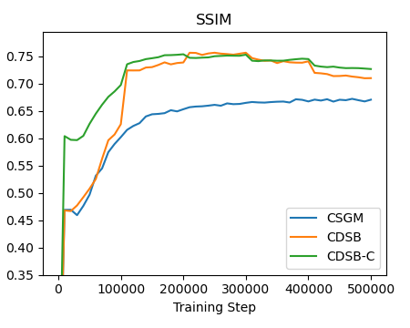
In standard SGMs and for the unconditional SB, we typically select $p_{\textup{ref}}(x)=\mathcal{N}(x;0,\sigma_{\textup{ref}}^{2}\operatorname{Id})$. However, initializing ancestral sampling from random noise to eventually obtain samples from $p(x|y)$ can be inefficient as $y$ already contains useful information about $X$. Fortunately, it is easy to use a joint reference measure of the form $p_{\textup{jref}}(x,y)=p_{\textup{ref}}(x|y)p_{\textup{obs}}(y)$ instead of $p_{\textup{jref}}(x,y)=p_{\textup{ref}}(x)p_{\textup{obs}}(y)$ in CSB and CDSB. The only modification in Algorithm 1 is that line 8 becomes $Y^{j}\sim p_{\textup{obs}}(y),X^{j}_{N}\sim p_{\textup{ref}}(x|Y^{j})$. In some interesting scenarios, we can select $p_{\textup{ref}}(x|y)$ as an approximation to $p(x|y)$ in order to accelerate the sampling process. This means we construct a CSB between $p(x|y)$ and its approximation $p_{\textup{ref}}(x|y)$, instead of between $p(x|y)$ and noise. We refer to this extension of CDSB as CDSB-C.

As a simple example, consider obtaining super-resolution (SR) image samples from a low-resolution image $Y=y$. Assume that $y$ has been suitably upsampled to have the same dimensionality as $X$. In this case, $y$ itself can serve as an approximate initialization for sampling $X_{N}$. A simple model is to take $p_{\textup{ref}}(x|y)=\mathcal{N}(x;y,\sigma_{\textup{ref}}^{2}\operatorname{Id})$ with $\sigma_{\textup{ref}}^{2}=\rho\sigma_{x|y}^{2}$, where $\rho$ is a variance inflation parameter and $\sigma_{x|y}^{2}$ is an estimate of the conditional variance of $X$ given $Y$. See Figure 1b for an illustration. In our experiments, we also explore other $p_{\textup{ref}}(x|y)$ obtained using the Ensemble Kalman Filter (EnKF) as well as neural network models.

5.2 Conditional Forward Process

To accelerate the convergence of IPF, we also have the flexibility to make the initial forward noising process dynamics dependent on $Y=y$, i.e. $p_{y}(x_{0:N})=p(x_{0}|y)\prod_{k=0}^{N-1}p_{k+1|k}(x_{k+1}|x_{k},y)$. As shown below, it is beneficial to initialize $p_{y}$ close to the CSB solution $\pi^{c,\star}_{y}$.

Proposition .

For any $n\in\mathbb{N}$ with $n\geq 1$, we have

$$\mathbb{E}[\operatorname{KL}(\pi^{c,n}_{Y,0}|p(\cdot|Y))]\leq\tfrac{2}{n}\mathbb{E}[\operatorname{KL}(\pi^{c,\star}_{Y}|p_{Y})],$$ (25)

where for any $n\in\mathbb{N}$, $\bar{\pi}^{n}=\bar{p}_{\textup{obs}}\otimes\pi^{c,n}$ is the $n^{\textup{th}}$ IPF iterate and the expectations are w.r.t. $Y\sim p_{\textup{obs}}$.

As a result, we should choose the initial forward noising process $p_{y}$ such that its terminal marginal $p_{y,N}$ targets $p_{\textup{ref}}(\cdot|y)$. However, contrary to diffusion models, we recall that our framework does not strictly require $p_{y,N}\approx p_{\textup{ref}}(\cdot|y)$ to provide approximate samples from the posterior of interest.

For tractable $p_{\textup{ref}}(x|y)$, we can define $p_{y}(x_{0:N})$ using an unadjusted Langevin dynamics; i.e. $p_{k+1|k}(x^{\prime}|x,y)=\mathcal{N}(x^{\prime};x+\gamma_{k+1}\nabla\log p_{\textup{ref}}(x|y),2\gamma_{k+1}\operatorname{Id})$. In the case $p_{\textup{ref}}(x|y)=\mathcal{N}(x;\mu(y),\sigma^{2}(y)\operatorname{Id})$, this reduces to a discretized Ornstein–Uhlenbeck process admitting $p_{\textup{ref}}(x|y)$ as limiting distribution as $\gamma\to 0$ and $N\to\infty$ [Durmus and Moulines, 2017].

5.3 Forward-Backward Sampling

When we use an unconditional $p_{\textup{ref}}(x)$, our proposed method also shares connections with the conditional transport methodology developed by Marzouk et al. [2016], Spantini et al. [2022]. They propose methods to learn a deterministic invertible transport map $\mathcal{S}(x,y):\mathcal{X}\times\mathcal{Y}\to\mathcal{X}$ which maps samples from $p(x|y)$ to $p_{\textup{ref}}(x)$. To sample from $p(x|y^{\textup{obs}})$, one samples $X^{\textup{ref}}\sim p_{\textup{ref}}(x)$, then transports back the sample through the inverse map $X^{\textup{pos}}={\mathcal{S}}(\cdot,y^{\textup{obs}})^{-1}(X^{\textup{ref}})$.

As noted by Spantini et al. [2022], an alternative method to sample from $p(x|y^{\textup{obs}})$ consists of first sampling $(X,Y)\sim p_{\textup{join}}$, then following the two-step transformation $\hat{X}^{\textup{ref}}=\mathcal{S}(X,Y),\leavevmode\nobreak\ \leavevmode\nobreak\ \hat{X}^{\textup{pos}}=\mathcal{S}(\cdot,y^{\textup{obs}})^{-1}(\hat{X}^{\textup{ref}})$. By definition of $\mathcal{S}$, $\hat{X}^{\textup{ref}}$ is also distributed according to $p_{\textup{ref}}$. However, since the transport map ${\mathcal{S}}$ may be imperfect in practice, this sampling strategy provides the advantage of cancellation of errors between $\mathcal{S}$ and $\mathcal{S}(\cdot,y^{\textup{obs}})^{-1}$.

We also explore an analogous forward-backward sampling scheme in our framework, which first samples $(X,Y)\sim p_{\textup{join}}$, followed by sampling $\hat{X}_{N}\sim\bar{p}^{L}_{N|0}(x_{N}|X,Y)$ through the forward half-bridge, then $\hat{X}_{0}\sim\bar{q}^{L}_{0|N}(x_{0}|\hat{X}_{N},y^{\textup{obs}})$ through the backward half-bridge. Since $\bar{q}^{L}$ is the approximate time-reversal of $\bar{p}^{L}$, this strategy shares similar advantages as the method of Spantini et al. [2022] when the half-bridge $\bar{q}^{L}(x_{0:N}|y^{\textup{obs}})$ does not solve the CSB problem exactly. We call this extension CDSB-FB.

6 Related work

Approximate Bayesian computation (ABC), also known as likelihood-free inference, has been developed to approximate the posterior when the likelihood is intractable but one can simulate synthetic data from it; see e.g.[Beaumont, 2019]. However, these methods typically require knowing the prior, while CDSB only needs to have access to joint samples and learns about the posterior directly. For tasks such as image inpainting, the prior is indeed implicit.

Schrödinger bridges techniques to perform both static and sequential Bayesian inference for state-space models have been developed by Bernton et al. [2019] and Reich [2019]. However, these methods require being able to evaluate pointwise an unnormalized version of the target posterior distribution contrary to the CDSB-based methods developed here.

Conditional transport. Performing conditional simulation by learning a transport map between joint distributions on $X,Y$ having the same $Y$-marginals (as $p_{\textup{join}}$ and $p_{\textup{ref}}$) has been first proposed by Marzouk et al. [2016]. Various techniques have been subsequently developed to approximate such maps such as polynomial or radial basis representations [Marzouk et al., 2016, Baptista et al., 2020], Generative Adversarial Networks [Kovachki et al., 2021, Zhou et al., 2022] or normalizing flows [Kruse et al., 2021]. CDSB also fits into this framework, but instead utilizes stochastic transport maps. Recently, Taghvaei and Hosseini [2022] have also proposed independently using conditional transport ideas to perform optimal filtering for state-space models.

Conditional SGMs. SGMs have been applied to perform posterior simulation, primarily for images, as described in Section 2.2 and references therein. An alternative line of work for image editing [Song and Ermon, 2019, Choi et al., 2021, Chung et al., 2021, Meng et al., 2022] utilizes the denoising property of SGMs to iteratively denoise noisy versions of a reference image $y$ while restricted to retain particular features of $y$. However, $p_{\textup{ref}}(x)=\mathcal{N}(x;0,\sigma_{\textup{ref}}^{2}\operatorname{Id})$ so image generation is started from noise and typically hundreds or thousands of refinement steps are required. Our framework can incorporate in a principled way information given by $y$ in the reverse process’s initialization (see Section 5.1). Recently Zheng et al. [2022], Lu et al. [2022] have also proposed suitable choices for $p_{\textup{ref}}(x)$ or $p_{\textup{ref}}(x|y)$ to shorten the diffusion process. In comparison, the CDSB framework is more flexible and allows for general $p_{\textup{ref}}(x|y)$ which can be non-Gaussian and different from the initial forward diffusion’s terminal distribution $p_{N}(x_{N}|y)$. For instance, we explore using noiseless pre-trained super-resolution models as $p_{\textup{ref}}(x|y)$ in Section 7.3.2, where CDSB further improves the SR samples closer to the data distribution. Finally, for linear Gaussian inverse problems, Kadkhodaie and Simoncelli [2021], Kawar et al. [2021, 2022] develop efficient methodologies using unconditional SGMs when the linear degradation model and the Gaussian noise level are known.

SGM acceleration techniques. Many techniques have been proposed to accelerate SGMs and CSGMs. For example, Luhman and Luhman [2021], Salimans and Ho [2022] propose to learn a distillation network on top of SGM models, while Song et al. [2021a] perform a subsampling of the timesteps in a variational setting. Watson et al. [2022] optimize the timesteps with a fixed budget using dynamic programming. Xiao et al. [2021] perform multi-steps denoising using GANs while Dockhorn et al. [2022] consider underdamped Langevin dynamics as forward process. We emphasize that many of these techniques are complementary to and can be readily applied in the SB setting; e.g.one could distill the last CDSB network $\mathbf{B}^{y}_{\theta^{L}}$. Additionally, SB and CSB provide a framework to perform few-step sampling.

7 Experiments

CSGM  

CDSB  

CDSB-FB  

MGAN  

Figure 2: True posterior $p(x|y^{\textup{obs}})$ for $y^{\textup{obs}}\in\{-1.2,0,1.2\}$ (solid lines) and approximations for the 2D examples.

		MCMC	CDSB	CDSB-FB	CDSB-C	MGAN	IT
Mean	$x_{1}$	.075	.066	.068	.072	.048	.034
	$x_{2}$	.875	.897	.897	.891	.918	.902
Var	$x_{1}$	.190	.184	.190	.188	.177	.206
	$x_{2}$	.397	.387	.391	.393	.419	.457
Skew	$x_{1}$	1.94	1.90	2.01	1.90	1.83	1.63
	$x_{2}$	.681	.591	.628	.596	.630	.872
Kurt	$x_{1}$	8.54	7.85	8.54	8.00	7.64	7.57
	$x_{2}$	3.44	3.33	3.51	3.27	3.19	3.88

Table 1: Estimated posterior moments for the BOD example. The closest estimates to MCMC are highlighted in bold.

7.1 2D Synthetic Examples

	$N=5$	$N=10$
CSGM	17.22/0.672	20.03/0.795
CDSB	18.55/0.746	20.69/0.792
CSGM-C	18.61/0.749	20.83/0.838
CDSB-C	19.67/0.753	20.95/0.840

(a)

$N=10$	$N=20$
14.77/0.599	16.31/0.706
16.24/0.618	16.61/0.657
16.38/0.701	16.53/0.730
16.60/0.700	16.65/0.747

(b)

$N=20$	$N=50$
19.52/0.471/92.02	20.52/0.567/48.68
19.72/0.504/57.22	20.70/0.590/40.08
20.44/0.566/44.44	20.84/0.592/22.89
21.11/0.614/28.41	21.46/0.646/13.71

(c)

$N=20$	$N=50$
24.22/0.844/17.62	25.29/0.878/7.18
24.88/0.850/19.85	26.61/0.894/3.87
28.26/0.914/3.63	28.14/0.913/1.31
28.19/0.915/2.28	28.06/0.914/1.14

(d)

Table 2: Results for (a) MNIST 4x SR; (b) MNIST 14x14 inpainting; (c) CelebA 4x SR with Gaussian noise; (d) CelebA 32x32 inpainting. Reported results are denoted in the format PSNR↑/SSIM↑(/FID↓).

(a) $y^{\textup{obs}}$

(b) Ground truth

(c) CSGM

(d) CDSB-C

Figure 3: Uncurated samples for the MNIST 4x SR task with $N=5$.

(a) $y^{\textup{obs}}$

(b) Ground truth

(c) CSGM

(d) CDSB-C

Figure 4: Uncurated samples for the CelebA 4x SR with Gaussian noise task with $N=20$.

We first demonstrate the validity and accuracy of our method using the two-dimensional examples of Kovachki et al. [2021]. We consider three nonlinear, non-Gaussian examples for $p_{\textup{join}}(x,y)$: define $p_{\textup{obs}}(y)=\textup{Unif}(y;[-3,3])$ for all examples and $p(x|y)$ is defined through

Example 1: $$X=\tanh(Y)+Z, Z\sim\Gamma(1,0.3),$$ (26)

Example 2: $$X=\tanh(Y+Z), Z\sim\mathcal{N}(0,0.05),$$ (27)

Example 3: $$X=Z\tanh(Y), Z\sim\Gamma(1,0.3).$$ (28)

We run CDSB on each of the examples with 50,000 training points and compare with the Monotone GAN (MGAN) algorithm [Kovachki et al., 2021]. CDSB uses a neural network model with 32k parameters (approximately 6x less parameters than MGAN) with $N=50$ diffusion steps. Figure 2 shows the resulting histogram of the learned $p(x|y^{\textup{obs}})$ and the true posterior for $y^{\textup{obs}}\in\{-1.2,0,1.2\}$. As can be observed, the empirical density of CDSB samples is sharper and aligns more closely with the ground truth density. We also observe that using more CDSB iterations corrects the sampling bias compared to using only one CDSB iteration (which corresponds to CSGM). Using forward-backward sampling (CDSB-FB) further improves the sample quality.

7.2 Biochemical Oxygen Demand Model

We now consider a Bayesian inference problem on biochemical oxygen demand (BOD) from Marzouk et al. [2016]. Let $X_{1},X_{2}\overset{\textup{i.i.d.}}{\sim}\mathcal{N}(0,1)$, $A=0.8+0.4\operatorname{erf}(X_{1}/\sqrt{2})$, $B=0.16+0.15\operatorname{erf}(X_{2}/\sqrt{2})$ and $Y=\{Y(t)\}_{t=1}^{5}$ satisfy $Y(t)=A(1-\exp(-Bt))+Z$ with $Z\sim\mathcal{N}(0,{10}^{-3})$. Table 1 displays moment statistics of the estimated posterior $p(x|y)$ (standard deviations are reported in the supplementary), in comparison with the “ground truth” statistics computed using $6\times{10}^{6}$ MCMC steps as reported in Marzouk et al. [2016]. To match the evaluation in Kovachki et al. [2021], the reported statistics are computed using 30,000 samples and averaged across the last 10 CDSB iterations. The resulting posterior displays high skewness and high kurtosis, but all CDSB-based methods achieve more accurate posterior estimation than MGAN and the inverse transport (IT) method in Marzouk et al. [2016].

7.3 Image Experiments

7.3.1 Gaussian Reference Measure

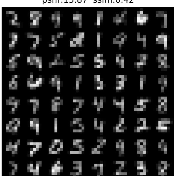
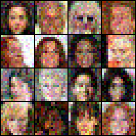
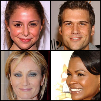
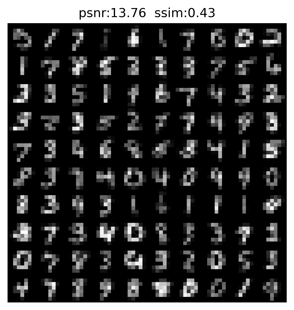
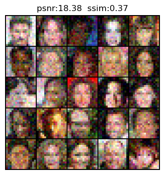
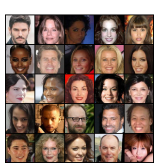
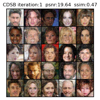
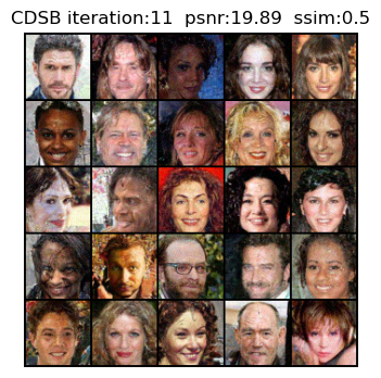
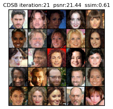
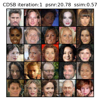
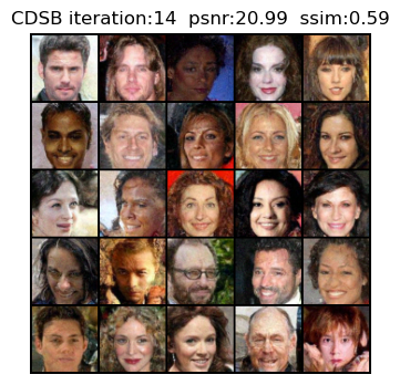
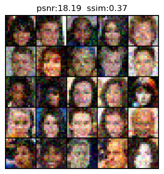
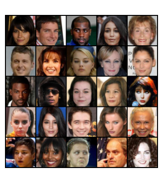
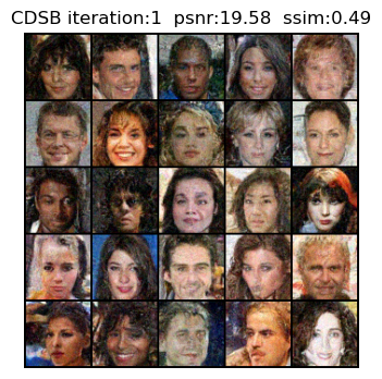
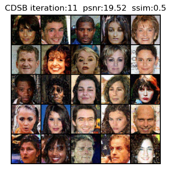
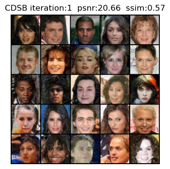
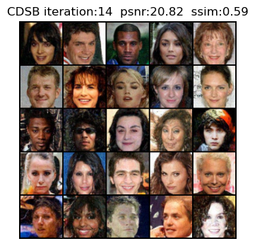
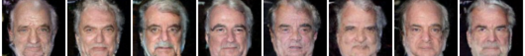
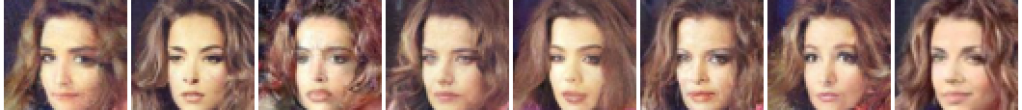
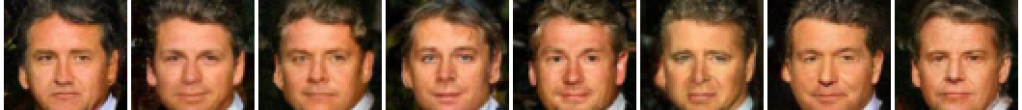
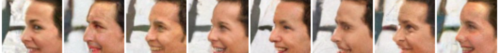
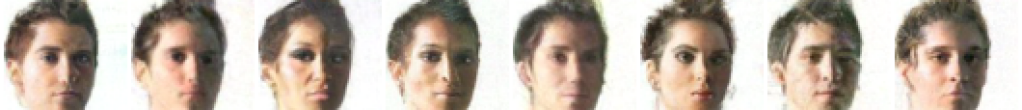
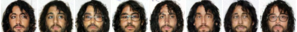
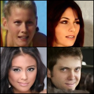
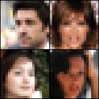
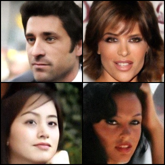
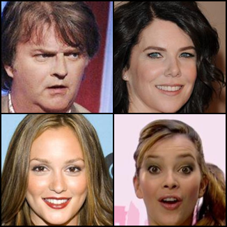
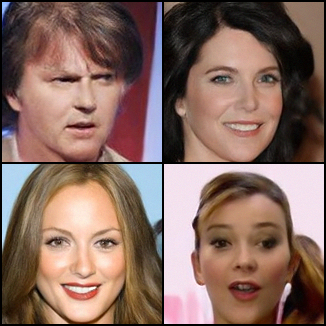
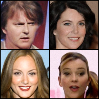
We now apply CDSB to a range of inverse problems on image datasets. We consider the following tasks: (a) MNIST 4x SR (7x7 to 28x28), (b) MNIST center 14x14 inpainting, (c) CelebA 4x SR (16x16 to 64x64) with Gaussian noise of $\sigma_{y}=0.1$, (d) CelebA center 32x32 inpainting. For CSGM-C and CDSB-C, we consider the following choices for conditional $p_{\textup{ref}}(x|y)$: for tasks (a) and (c), we use the upsampled $y$ directly as described in Section 5.1; for inpainting tasks (b) and (d), we use a separate neural network with the same architecture as $\mathbf{F},\mathbf{B}$ to output the initialization mean. In Table 2 we report PSNR and SSIM (the higher the better), as well as FID scores (the lower the better) for RGB images only. We display a visual comparison between the methods in Figures 4 and 4, and additional image samples in the supplementary. CDSB and CDSB-C both provide significant improvement in terms of quantitative metrics as well as visual evaluations, and high-quality images can be generated quickly under few iterations $N$.

7.3.2 Pre-trained SR Model for Reference Measure

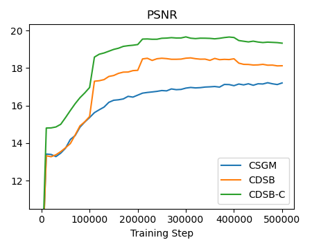
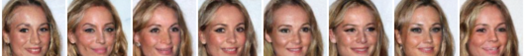
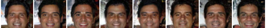
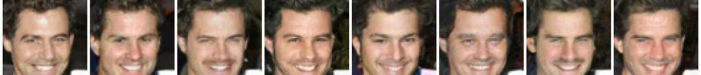
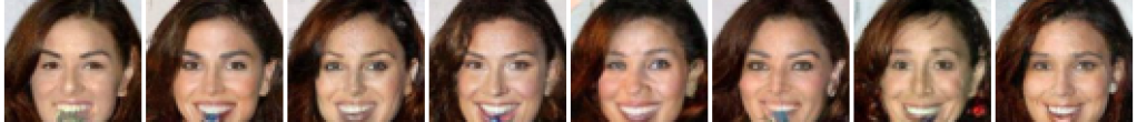
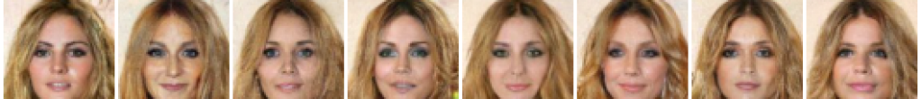
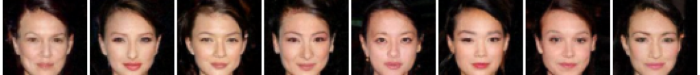
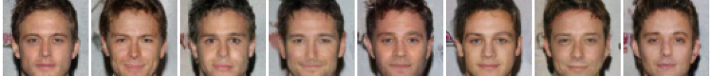
We further explore here the possibility of using a non-Gaussian $p_{\textup{ref}}(x|y)$ to further bridge the gap towards the true posterior $p(x|y)$. We utilize the super-resolution model SRFlow [Lugmayr et al., 2020], which produces a probability distribution over possible SR images using a conditional normalizing flow. We use their pre-trained model checkpoints for the 8x SR task for CelebA (160x160). We then train a short CDSB model with SRFlow as $p_{\textup{ref}}(x|y)$, in order to take advantage of the high sampling quality of diffusion models. As can be seen from Figure 5, with only $N=10$ steps the CDSB model is able to make meaningful improvements to the SRFlow samples, especially in the finer details such as facial features and hair texture. Quantitatively, CDSB-C produces significant improvement over the FID score at the cost of a decrease in PSNR; see Table 3. Note that this choice of non-Gaussian $p_{\textup{ref}}(x|y)$ is not compatible with CSGM. Interestingly CSGM-C still improves the PSNR compared to SRFlow, but produces worse FID scores than CDSB-C and blurry samples.

$p_{\textup{ref}}(x|y)$	CSGM-C	CDSB-C
Gaussian	22.21/0.521/87.02	23.86/0.628/31.65
SRFlow $\tau=0.8$	24.97/0.701/26.83	24.34/0.674/15.00
SRFlow $\tau=0.8$	24.83/0.702/30.92

Table 3: Results for CelebA 8x SR. Reported results are denoted in the format PSNR↑/SSIM↑/FID↓. The final row reports our evaluated results of the SRFlow model.

(a) $y^{\textup{obs}}$

(b) Ground truth

(c) SRFlow

(d) CDSB-C

Figure 5: Paired samples for CelebA 8x SR. The SRFlow samples (c) are inputted as conditional initialization into CDSB-C (d), which produces fine modifications over $N=10$ steps (Best viewed when zoomed in).

7.4 Filtering in State-Space Models

Consider a state-space model defined by a bivariate Markov chain $(X_{t},Y_{t})_{t\geq 1}$ of initial density $\mu(x_{1})g(y_{1}|x_{1})$ and transition density $f(x_{t+1}|x_{t})g(y_{t+1}|x_{t+1})$ where $X_{t}$ is latent while $Y_{t}$ is observed. We are interested in estimating sequentially in time the filtering distribution $p(x_{t}|y^{\textup{obs}}_{1:t})$, that is the posterior of $X_{t}$ given the observations $Y_{1:t}=y^{\textup{obs}}_{1:t}$. We show here how CDSB can be used at each time $t$ to obtain a sample approximation of these filtering distributions. This CDSB-based algorithm only requires us being able to sample from the transition density $f(x_{t+1}|x_{t})g(y_{t+1}|x_{t+1})$ and is thus more generally applicable than standard techniques such as particle filters [Doucet and Johansen, 2009].

Assume at time $t$, one has a collection of samples $\{X^{i}_{t}\}_{i=1}^{M}$ distributed (approximately) according to $p(x_{t}|y^{\textup{obs}}_{1:t})$. We sample $X^{i}_{t+1}\sim f(x_{t+1}|X^{i}_{t})$ and $Y^{i}_{t+1}\sim g(y_{t+1}|X^{i}_{t+1})$. The resulting samples $\{X^{i}_{t+1},Y^{i}_{t+1}\}_{i=1}^{M}$ are thus distributed according to $p_{\textup{join}}(x_{t+1},y_{t+1}):=p(x_{t+1},y_{t+1}|y^{\textup{obs}}_{1:t})$. We can also easily obtain samples from $p_{\textup{jref}}(x_{t+1},y_{t+1}):=p_{\textup{ref}}(x_{t+1}|y_{t+1},y^{\textup{obs}}_{1:t})p(y_{t+1}|y^{\textup{obs}}_{1:t})$ where $p_{\textup{ref}}(x_{t+1}|y_{t+1},y^{\textup{obs}}_{1:t})$ is an easy-to-sample distribution designed by the user. Thus we can use CDSB to obtain a (stochastic) transport map between $p_{\textup{join}}(x_{t+1},y_{t+1})$ and $p_{\textup{jref}}(x_{t+1},y_{t+1})$ and applying it to $Y_{t+1}=y^{\textup{obs}}_{t+1}$, we can obtain new samples from $p(x_{t+1}|y^{\textup{obs}}_{1:t+1})$. A similar strategy for filtering based on deterministic transport maps was recently proposed by Spantini et al. [2022].

We apply CSGM and CDSB to the Lorenz-63 model [Law et al., 2015] following the procedure above for a time series of length 2000. We consider a short diffusion process with $N=20$ steps, as well as a long one with $N=100$. To accelerate the sequential inference process, in this example we use analytic basis regression instead of neural networks for all methods, and we only run 5 iterations of CDSB. As the EnKF is applicable to this model, we can use the resulting approximate Gaussian filtering distribution it outputs for $p_{\textup{ref}}(x_{t+1}|y_{t+1},y^{\textup{obs}}_{1:t})$ in CSGM-C and CDSB-C.

Table 4 shows that for $N=20$ both CDSB and CDSB-C successfully perform filtering and outperform the EnKF, whereas both CSGM and CSGM-C fail to track the state accurately and diverge after a few hundred times steps. CDSB-C achieves the lowest error consistently. When using $N=100$, CSGM can achieve RMSE comparable with CDSB-C using $N=20$, but CDSB still provides advantages compared to CSGM. CSGM-C achieves comparable RMSE as CDSB-C with suitably long diffusion process in this case. For lower ensemble size, e.g. $M=200$, occasional large errors occur for some of the runs; see supplementary for details. We conjecture that this is due to overfitting.

$M$	500	1000	2000
EnKF	.354±0.006	.355±.005	.354±.003
CSGM(-C) (short)	Diverges
CDSB (short)	.251±.011	.218±.008	.196±.005
CDSB-C (short)	.236±.012	.207±.014	.178±.007
CSGM (long)	.232±.008	.203±.009	.182±.009
CDSB (long)	.220±.012	.195±.007	.166±.004
CSGM-C (long)	.210±.009	.185±.005	.162±.004
CDSB-C (long)	.218±.014	.185±.008	.160±.003

Table 4: RMSEs over 10 runs between each algorithm’s filtering means and the ground truth filtering means for $N=20$ (short) and $N=100$ (long).

8 Discussion

We have proposed a SB formulation of conditional simulation and an algorithm, CDSB, to approximate its solution. The first iteration of CDSB coincides with CSGM while subsequent ones can be thought of as refining it. This theoretically grounded approach is complementary to the many other techniques that have been recently proposed to accelerate SGMs and could be used in conjunction with them. However, it also suffers from limitations. As CDSB approximates numerically the diffusion processes output by IPF, the minimum $N$ one can pick to obtain reliable approximations is related to the steepness of the drift of these iterates which is practically unknown. Additionally CSGM and CDSB are only using $y^{\textup{obs}}$ when we want to sample from $p(x|y^{\textup{obs}})$ but not at the training stage. Hence if $y^{\textup{obs}}$ is not an observation “typical” under $p_{\textup{obs}}(y)$, the approximation of the posterior can be unreliable. In the ABC context, the best available methods rely on procedures which sample synthetic observations in the neighbourhood of $y^{\textup{obs}}$. It would be interesting but challenging to extend such ideas to CSGM and CDSB. Other interesting potential extensions include developing an amortized version of CDSB for filtering that would avoid having to solve a SB problem at each time step, and a conditional version of the multimarginal SB problem.

Appendix A Organization of the supplementary

The supplementary is organized as follows. We recall the DSB algorithm for unconditional simulation from De Bortoli et al. [2021] in Appendix B. The proofs of our propositions are given in Appendix C. In Appendix D, we give details on the loss functions we use to train CDSB. A continuous-time version of the conditional time-reversal and conditional DSB is presented in Appendix E. The forward-backward technique used in our experiments is detailed in Appendix F. Finally, we provide experimental details and guidelines in Appendix G.

Appendix B Diffusion Schrödinger bridge

We recall here the DSB algorithm introduced by De Bortoli et al. [2021] which is a numerical approximation of IPF.

Algorithm 2 Diffusion Schrödinger Bridge [De Bortoli et al., 2021]

1:  for $n\in\{0,\dots,L\}$ do

2:     while not converged do

3:        Sample $\{X^{j}_{k}\}_{k,j=0}^{N,M}$, where $X^{j}_{0}\sim p_{\textup{data}}$, and $X^{j}_{k+1}=\mathbf{F}_{\phi^{n}}(k,X^{j}_{k})+\sqrt{2\gamma_{k+1}}Z^{j}_{k+1}$

4:        Compute $\hat{\ell}^{b}_{n}(\theta^{n})$ approximating (29)

5:        $\theta^{n}\leftarrow\textrm{Gradient Step}(\hat{\ell}^{b}_{n}(\theta^{n}))$

6:     end while

7:     while not converged do

8:        Sample $\{X^{j}_{k}\}_{k,j=0}^{N,M}$, where $X^{j}_{N}\sim p_{\textup{ref}}$, and $X^{j}_{k-1}=\mathbf{B}_{\theta^{n}}(k,X^{j}_{k})+\sqrt{2\gamma_{k}}\tilde{Z}^{j}_{k}$

9:        Compute $\hat{\ell}^{f}_{n+1}(\phi^{n+1})$ approximating (30)

10:        $\phi^{n+1}\leftarrow\textrm{Gradient Step}(\hat{\ell}^{f}_{n+1}(\phi^{n+1}))$

11:     end while

12:  end for

13:  Output: $(\theta^{L},\phi^{L+1})$

In this (unconditional) SB scenario, the transition kernels satisfy $q^{n}_{k|k+1}(x|x^{\prime})=\mathcal{N}(x;\mathbf{B}_{\theta^{n}}(k+1,x^{\prime}),2\gamma_{k+1}\operatorname{Id})$ and $p_{k+1|k}^{n}(x^{\prime}|x)=\mathcal{N}(x^{\prime};\mathbf{F}_{\phi^{n}}(k,x),2\gamma_{k+1}\operatorname{Id})$ where $\theta^{n}$ is obtained by minimizing

$$\textstyle{\ell^{b}_{n}(\theta)=\mathbb{E}_{p^{n}}[\sum_{k}\|\mathbf{B}_{\theta}(k+1,X_{k+1})-G_{n,k}(X_{k},X_{k+1})\|^{2}]}$$ (29)

for $G_{n,k}(x,x^{\prime})=x^{\prime}+\mathbf{F}_{\phi^{n}}(k,x)-\mathbf{F}_{\phi^{n}}(k,x^{\prime})$ and $\phi^{n+1}$ by minimizing

$$\textstyle{\ell^{f}_{n+1}(\phi)=\mathbb{E}_{q^{n}}[\sum_{k}\|\mathbf{F}_{\phi}(k,X_{k})-H_{n,k}(X_{k},X_{k+1})\|^{2}]}$$ (30)

for $H_{n,k}(x,x^{\prime})=x+\mathbf{B}_{\theta^{n}}(k+1,x^{\prime})-\mathbf{B}_{\theta^{n}}(k+1,x)$. See De Bortoli et al. [2021] for a derivation of these loss functions.

Appendix C Proofs of Propositions

C.1 Proof of Proposition 4

Let $\bar{\pi}$ such that $\textup{KL}(\bar{\pi}|\bar{p})<+\infty$, which exists since we have that $\textup{KL}(\bar{\pi}^{\star}|\bar{p})<+\infty$, and $\bar{\pi}_{0}=p_{\textup{join}},\leavevmode\nobreak\ \bar{\pi}_{N}=p_{\textup{jref}}$, where we define the joint forward process $\bar{p}(x_{0:N},y_{0:N}):=p_{y_{0}}(x_{0:N})\bar{p}_{\textup{obs}}(y_{0:N})$. Recall that $p_{y_{0}}(x_{0:n}):=p(x_{0}|y_{0})\prod_{k=0}^{N-1}p_{k+1|k}(x_{k+1}|x_{k})$ is the forward process starting from the posterior $p(x_{0}|y_{0})$, and $\bar{p}_{\textup{obs}}(y_{0:N}):=p_{\textup{obs}}(y_{0})\prod_{k=0}^{N-1}\delta_{y_{k}}(y_{k+1})$ is the extended $y$-process. Since $\operatorname{KL}(\bar{\pi}|\bar{p})<+\infty$ we have using the transfer theorem [Kullback, 1997, Theorem 2.4.1] that $\operatorname{KL}(\bar{\pi}_{\textup{obs}}|\bar{p}_{\textup{obs}})<+\infty$, where $\bar{\pi}_{\textup{obs}}(y_{0:N}):=\int_{(\mathbb{R}^{d})^{N}}\bar{\pi}(x_{0:N},y_{0:N})\mathrm{d}x_{0:N}$. In addition, using the chain rule for the Kullback–Leibler divergence, see [Léonard, 2014, Theorem 2.4], we get that

$$\textstyle{\operatorname{KL}(\bar{\pi}_{\textup{obs}}|\bar{p}_{\textup{obs}})=\operatorname{KL}(\bar{\pi}_{\textup{obs},0}|p_{\textup{obs}})+\int_{\mathcal{Y}}\operatorname{KL}(\bar{\pi}_{\textup{obs}|0}|\bar{p}_{\textup{obs}|0})p_{\textup{obs}}(y)\mathrm{d}y<+\infty},$$ (31)

where $\bar{p}_{\textup{obs}|0}=\prod_{k=0}^{N-1}\delta_{y_{k}}(y_{k+1})$ and therefore $\bar{\pi}_{\textup{obs}|0}=\bar{p}_{\textup{obs}|0}$. Since we also have that $\bar{\pi}_{\textup{obs},0}=p_{\textup{obs}}$ we get that $\bar{\pi}_{\textup{obs}}=\bar{p}_{\textup{obs}}$. Hence, letting $\pi^{c}$ be the kernel such that $\bar{\pi}=\pi^{c}\otimes\bar{p}_{\textup{obs}}$ we have using [Léonard, 2014, Theorem 2.4] that

$$\textstyle{\operatorname{KL}(\bar{\pi}|\bar{p})=\int_{\mathcal{Y}}\operatorname{KL}\left(\pi^{c}_{y}|p_{y}\right)p_{\textup{obs}}(y)\mathrm{d}y.}$$ (32)

In addition, we have $\bar{\pi}_{0}=\pi_{0}^{c}\otimes p_{\textup{obs}}=p_{\textup{join}}$. Similarly, we have $\bar{\pi}_{N}=\pi_{N}^{c}\otimes p_{\textup{obs}}=p_{\textup{jref}}$. Hence, $\pi_{y,0}^{c}=p(\cdot|y)$ and $\pi_{y,N}^{c}=p_{\textup{ref}}$, $p_{\textup{obs}}$-almost surely. Let $\bar{\pi}^{\star}=\pi^{\star,c}\otimes\bar{p}_{\textup{obs}}$ be the minimizer of (18) and $\hat{\pi}^{c}$ be the minimizer of (17). Then, we have that $\bar{\pi}=\hat{\pi}^{c}\otimes\bar{p}_{\textup{obs}}$ satisfies $\operatorname{KL}(\bar{\pi}^{\star}|\bar{p})\leq\operatorname{KL}(\bar{\pi}|\bar{p})$. Using (32), we have that $\mathbb{E}[\operatorname{KL}\left(\pi^{\star,c}_{Y}|p_{Y}\right)]\leq\mathbb{E}[\operatorname{KL}\left(\hat{\pi}^{c}_{Y}|p_{Y}\right)]$. But we have that $\mathbb{E}[\operatorname{KL}\left(\hat{\pi}^{c}_{Y}|p_{Y}\right)]\leq\mathbb{E}[\operatorname{KL}\left(\pi^{\star,c}_{Y}|p_{Y}\right)]$ since $\hat{\pi}^{c}$ is the minimizer of (17). Using the uniqueness of the minimizer of (17) we have that $\pi^{\star,c}=\hat{\pi}^{c}$, which concludes the proof.

C.2 Proof of Proposition 4

Let $n\in\mathbb{N}$ and $\bar{q}$ be such that $\operatorname{KL}(\bar{q}|\bar{p}^{n})<+\infty$ and $\bar{q}_{N}=p_{\textup{jref}}$ (note that the existence of such a distribution is ensured since $\operatorname{KL}(p_{\textup{join}}\otimes p_{\textup{jref}}|\bar{p}^{n}_{0,N})<+\infty$). Using the chain rule for the Kullback–Leibler divergence, see [Léonard, 2014, Theorem 2], we have

$$\textstyle{\operatorname{KL}(\bar{q}|\bar{p}^{n})=\operatorname{KL}\left(\bar{q}_{\textup{obs}}|\bar{p}_{\textup{obs}}\right)+\int_{\mathcal{Y}^{N+1}}\operatorname{KL}(\bar{q}_{|\textup{obs}}|\bar{p}_{|\textup{obs}}^{n})\mathrm{d}\bar{q}_{\textup{obs}}(y_{0:N}),}$$ (33)

where $\bar{q}_{\textup{obs}}=\int_{\mathcal{X}^{N+1}}\bar{q}(x_{0:N},y_{0:N})\mathrm{d}x_{0:N}$ and $\bar{q}_{|\textup{obs}}$ and $\bar{p}_{|\textup{obs}}^{n}$ are the conditional distribution of $\bar{q}$, respectively $\bar{p}^{n}$ w.r.t. to $y_{0:N}$. Since $\operatorname{KL}\left(\bar{q}_{\textup{obs}}|\bar{p}_{\textup{obs}}\right)<+\infty$, we can use [Léonard, 2014, Theorem 2.4] and we have

$$\textstyle{\operatorname{KL}\left(\bar{q}_{\textup{obs}}|\bar{p}_{\textup{obs}}\right)=\operatorname{KL}\left(\bar{q}_{\textup{obs},N}|\bar{p}_{\textup{obs},N}\right)+\int_{\mathcal{Y}}\operatorname{KL}\left(\bar{q}_{\textup{obs}|N}|\bar{p}_{\textup{obs}|N}\right)\mathrm{d}\bar{q}_{\textup{obs},N}(y_{N}),}$$ (34)

with $\bar{p}_{\textup{obs}|N}(y_{0:N-1}|y_{N})=\prod_{k=0}^{N-1}\delta_{y_{k+1}}(y_{k})$. Therefore, since $\operatorname{KL}\left(\bar{q}_{\textup{obs}}|\bar{p}_{\textup{obs}}\right)<+\infty$, we get that $\bar{q}_{\textup{obs}|N}(y_{0:N-1}|y_{N})=\prod_{k=0}^{N-1}\delta_{y_{k+1}}(y_{k})$. Since $\bar{q}_{\textup{obs},N}=p_{\textup{obs}}$, we get that $\bar{q}(x_{0:N},y_{0:N})=\bar{p}_{\textup{obs}}(y_{0:N})\bar{q}(x_{0:N}|y_{0:N})=\bar{p}_{\textup{obs}}(y_{0:N})\bar{q}(x_{0:N}|y_{N})$, where we have used that $y_{N}=y_{k}$ for $k\in\{0,\dots,N\}$, $\bar{p}_{\textup{obs}}(y_{0:N})$ almost surely. Combining this result and (33) we get that

$$\operatorname{KL}(\bar{q}|\bar{p}^{n}) =\textstyle{\int_{\mathcal{Y}^{N+1}}\operatorname{KL}(\bar{q}_{|\textup{obs}}|\bar{p}_{|\textup{obs}}^{n})\mathrm{d}p_{\textup{obs}}(y_{0:N})}=\textstyle{\int_{\mathcal{Y}}\operatorname{KL}(\bar{q}(\cdot|y_{N})|\bar{p}^{n}(\cdot|y_{N}))\mathrm{d}p_{\textup{obs}}(y_{N}),}$$ (35)

Using [Léonard, 2014, Theorem 2], we have that for any $y_{N}\in\mathcal{Y}$

$$\textstyle{\operatorname{KL}(\bar{q}(\cdot|y_{N})|\bar{p}^{n}(\cdot|y_{N})=\operatorname{KL}(p_{\textup{ref}}|\bar{p}_{N}^{n}(\cdot|y_{N}))+\int_{\mathcal{Y}}\operatorname{KL}(\bar{q}(\cdot|y_{N},x_{N})|\bar{p}^{n}(\cdot|y_{N},x_{N}))p_{\textup{ref}}(x_{N})\mathrm{d}x_{N}.}$$ (36)

For the IPF solution $\bar{q}^{n}$, we get that $\bar{q}^{n}(\cdot|y_{N},x_{N})=\bar{p}^{n}(\cdot|y_{N},x_{N})$. Therefore for any $x_{0:N}\in\mathcal{X}^{N+1}$ and $y_{N}\in\mathcal{Y}$,

$$\textstyle{\bar{q}^{n}(x_{0:N}|y_{N})=p_{\textup{ref}}(x_{N})\prod_{k=0}^{N-1}\bar{p}^{n}_{k|k+1}(x_{k}|x_{k+1},y_{N})}.$$ (37)

The proof is similar for any $x_{0:N}\in\mathcal{X}^{N+1}$ and $y_{0}\in\mathcal{Y}$, we have

$$\textstyle{\bar{p}^{n+1}(x_{0:N}|y_{0})=p(x_{0}|y_{0})\prod_{k=0}^{N-1}\bar{q}^{n}_{k+1|k}(x_{k+1}|x_{k},y_{0}).}$$ (38)

C.3 Proof of Proposition 5.2

Using [Léger, 2021, Corollary 1], we get that for any $n\in\mathbb{N}$ with $n\geq 1$

$$\operatorname{KL}(\bar{\pi}^{n}_{0}|p_{\textup{join}})+\operatorname{KL}(\bar{\pi}^{n}_{N}|p_{\textup{jref}})\leq\frac{2}{n}\operatorname{KL}(\bar{\pi}^{\star}|\bar{p}).$$ (39)

Similarly to Section 4, we have that for any $n\in\mathbb{N}$, there exists a Markov kernel $\pi^{c,n}$ such that $\bar{\pi}^{n}=\bar{p}_{\textup{obs}}\otimes\pi^{c,n}$. Recall that there exists a Markov kernel $\pi^{c,\star}$ such that $\bar{\pi}^{\star}=\bar{p}_{\textup{obs}}\otimes\pi^{c,\star}$ and that $\bar{p}=\bar{p}_{\textup{obs}}\otimes p_{y}$. Hence, using [Léonard, 2014, Theorem 2.4], we get that for any $n\in\mathbb{N}$,

$$\operatorname{KL}(\bar{\pi}^{n}_{0}|p_{\textup{join}})=\mathbb{E}[\operatorname{KL}(\pi^{c,n}_{Y,0}|p(\cdot|Y))],\qquad\operatorname{KL}(\bar{\pi}^{n}_{N}|p_{\textup{jref}})=\mathbb{E}[\operatorname{KL}(\pi^{c,n}_{Y,N}|p_{\textup{ref}})].$$ (40)

Similarly, we have that

$$\operatorname{KL}(\bar{\pi}^{\star}|\bar{p})=\mathbb{E}[\operatorname{KL}(\pi^{c,\star}_{Y}|p_{Y})].$$ (41)

We conclude the proof upon combining (39), (40) and (41).

Appendix D Details on the loss functions

In this section, we simplify notation and write $Y$ for all the random variables $Y_{0},Y_{1},...,Y_{N}$ as they are all equal almost surely under $\bar{p}^{n}$ and $\bar{q}^{n}$, similarly to Section 4. In Section 4, the transitions satisfy $\bar{q}^{n}_{k|k+1}(x|x^{\prime},y)=\mathcal{N}(x;\mathbf{B}^{y}_{\theta^{n}}(k+1,x^{\prime}),2\gamma_{k+1}\operatorname{Id})$ and $\bar{p}_{k+1|k}^{n}(x^{\prime}|x,y)=\mathcal{N}(x^{\prime};\mathbf{F}^{y}_{\phi^{n}}(k,x),2\gamma_{k+1}\operatorname{Id})$ where $\theta^{n}$ is obtained by minimizing

$$\textstyle{\ell^{b}_{n}(\theta)=\mathbb{E}_{\bar{p}^{n}}[\sum_{k}\|\mathbf{B}_{\theta}^{Y}(k+1,X_{k+1})-G_{n,k}^{Y}(X_{k},X_{k+1})\|^{2}]}$$ (42)

for $G_{n,k}^{y}(x,x^{\prime})=x^{\prime}+\mathbf{F}^{y}_{\phi^{n}}(k,x)-\mathbf{F}^{y}_{\phi^{n}}(k,x^{\prime})$ and $\phi^{n+1}$ by minimizing

$$\textstyle{\ell^{f}_{n+1}(\phi)=\mathbb{E}_{\bar{q}^{n}}[\sum_{k}\|\mathbf{F}_{\phi}^{Y}(k,X_{k})-H_{n,k}^{Y}(X_{k},X_{k+1})\|^{2}]}$$ (43)

for $H_{n,k}^{y}(x,x^{\prime})=x+\mathbf{B}^{y}_{\theta^{n}}(k+1,x^{\prime})-\mathbf{B}^{y}_{\theta^{n}}(k+1,x)$. We justify these formulas by proving the following result which is a straightforward extension of De Bortoli et al. [2021]. We recall that for any $n\in\mathbb{N}$, $k\in\{0,\dots,N\}$, $x_{k},x_{k+1}\in\mathbb{R}^{d}$ and $y\in\mathcal{Y}$, $b^{n,y}_{k+1}(x_{k+1})=-f^{n,y}_{k}(x_{k+1})+2\nabla\log\bar{p}^{n}_{k+1}(x_{k+1}|y)$ and $f^{n+1,y}_{k}(x_{k})=-b^{n,y}_{k+1}(x_{k})+2\nabla\log\bar{q}^{n}_{k}(x_{k}|y)$.

Proposition .

Assume that for any $n\in\mathbb{N}$ and $k\in\{0,\dots,N-1\}$, $\bar{q}_{k}(\cdot|y)$ and $\bar{p}_{k}(\cdot|y)$ are bounded and

$$\bar{q}_{k|k+1}^{n}(x_{k}|x_{k+1},y)=\mathcal{N}(x_{k};B_{k+1}^{n,y}(x_{k+1}),2\gamma_{k+1}\operatorname{Id}),\ \bar{p}_{k+1|k}^{n}(x_{k+1}|x_{k},y)=\mathcal{N}(x_{k+1};F_{k}^{n,y}(x_{k}),2\gamma_{k+1}\operatorname{Id}),$$ (44)

with $B^{n,y}_{k+1}(x)=x+\gamma_{k+1}b^{n,y}_{k+1}(x)$, $F^{n,y}_{k}(x)=x+\gamma_{k+1}f_{k}^{n,y}(x)$ for any $x\in\mathbb{R}^{d}$. Then we have for any $n\in\mathbb{N}$ and $k\in\{0,\dots,N-1\}$

$$\textstyle{B^{n}_{k+1}=\operatorname*{arg\,min}_{\mathrm{B}\in\mathrm{L}^{2}(\mathbb{R}^{d}\times\mathcal{Y},\mathbb{R}^{d})}\mathbb{E}_{\bar{p}^{n}}[\|\mathrm{B}(X_{k+1},Y)-G_{n,k}^{Y}(X_{k},X_{k+1})\|^{2}]},$$ (45)

$$\textstyle{F^{n+1}_{k}=\operatorname*{arg\,min}_{\mathrm{F}\in\mathrm{L}^{2}(\mathbb{R}^{d}\times\mathcal{Y},\mathbb{R}^{d})}\mathbb{E}_{\bar{q}^{n}}[\|\mathrm{F}(X_{k},Y)-H_{n,k}^{Y}(X_{k},X_{k+1})\|^{2}]},$$ (46)

$$G_{n,k}^{y}(x,x^{\prime})=x^{\prime}+F^{n,y}_{k}(x)-F^{n,y}_{k}(x^{\prime}),\qquad H_{n,k}^{y}(x,x^{\prime})=x+B^{n,y}_{k+1}(x^{\prime})-B^{n,y}_{k+1}(x).$$ (47)

Proof.

We only prove (45) since the proof (46) is similar. Let $n\in\mathbb{N}$ and $k\in\{0,\dots,N-1\}$. For any $x_{k+1}\in\mathbb{R}^{d}$ we have

$$\textstyle{\bar{p}^{n}_{k+1}(x_{k+1}|y)=(4\uppi\gamma_{k+1})^{-d/2}\int_{\mathbb{R}^{d}}\bar{p}^{n}(x_{k}|y)\exp[-\|F_{k}^{n,y}(x_{k})-x_{k+1}\|^{2}/(4\gamma_{k+1})]\mathrm{d}x_{k},}$$ (48)

with $F_{k}^{n,y}(x_{k})=x_{k}+\gamma_{k+1}f_{k}^{n,y}(x_{k})$. Since $\bar{p}^{n}_{k}>0$ is bounded using the dominated convergence theorem we have for any $x_{k+1}\in\mathbb{R}^{d}$

$$\textstyle{\nabla_{x_{k+1}}\log\bar{p}^{n}_{k+1}(x_{k+1}|y)=\int_{\mathbb{R}^{d}}(F_{k}^{n,y}(x_{k})-x_{k+1})/(2\gamma_{k+1})\leavevmode\nobreak\ \bar{p}_{k|k+1}(x_{k}|x_{k+1},y)\mathrm{d}x_{k}.}$$ (49)

Therefore we get that for any $x_{k+1}\in\mathbb{R}^{d}$

$$\textstyle{b_{k+1}^{n,y}(x_{k+1})=\int_{\mathbb{R}^{d}}(F_{k}^{n,y}(x_{k})-F_{k}^{n,y}(x_{k+1}))/\gamma_{k+1}\leavevmode\nobreak\ \bar{p}_{k|k+1}(x_{k}|x_{k+1},y)\mathrm{d}x_{k}.}$$ (50)

This is equivalent to

$$\textstyle{B_{k+1}^{n,y}(x_{k+1})={\mathbb{E}}[X_{k+1}+F_{k}^{n,Y}(X_{k})-F_{k}^{n,Y}(X_{k+1})|X_{k+1}=x_{k+1},Y=y]},$$ (51)

Hence, we get that

$$\textstyle{B^{n}_{k+1}=\operatorname*{arg\,min}_{\mathrm{B}\in\mathrm{L}^{2}(\mathbb{R}^{d}\times\mathcal{Y},\mathbb{R}^{d})}\mathbb{E}_{\bar{p}^{n}}[\|\mathrm{B}(X_{k+1},Y)-(X_{k+1}+F^{n,Y}_{k}(X_{k})-F^{n,Y}_{k}(X_{k+1}))\|^{2}]},$$ (52)

which concludes the proof. ∎

Appendix E Continuous-time versions of CSGM and CDSB

In the following section, we consider the continuous-time version of CSGM and CDSB. The continuous-time dynamics we recover can be seen as the extensions of the continuous-time dynamics obtained in the unconditional setting, see Song et al. [2021b], De Bortoli et al. [2021].

E.1 Notation

We start by introducing a few notations. The space of continuous functions from $\left[0,T\right]$ to $\mathbb{R}^{d}\times\mathcal{Y}$ is denoted $\mathcal{C}=\mathrm{C}(\left[0,T\right],\mathbb{R}^{d}\times\mathcal{Y})$ and we denote $\mathscr{P}(\mathcal{C})$ the set of probability measures defined on $\mathcal{C}$. A probability measure $\mathbb{P}\in\mathscr{P}(\mathcal{C})$ is associated with a diffusion if it is a solution to a martingale problem, i.e. $\mathbb{P}\in\mathscr{P}(\mathcal{C})$ is associated with $\mathrm{d}\mathbf{X}_{t}=b(t,\mathbf{X}_{t})\mathrm{d}t+\sqrt{2}\mathrm{d}\mathbf{B}_{t}$ if for any $\varphi\in\mathrm{C}_{c}^{2}(\mathbb{R}^{d},\mathbb{R})$, $(\mathbf{Z}_{t}^{\varphi})_{t\in\left[0,T\right]}$ is a $\mathbb{P}$-local martingale, where for any $t\in\left[0,T\right]$

$$\textstyle{\mathbf{Z}_{t}^{\varphi}=\varphi(\mathbf{X}_{t})-\int_{0}^{t}\mathcal{A}_{s}(\varphi)(\mathbf{X}_{s})\mathrm{d}s},\qquad\mathcal{A}_{t}(\varphi)(x)=\langle b(t,x),\nabla\varphi(x)\rangle+\Delta\varphi(x).$$ (53)

Here $\mathrm{C}_{c}^{2}(\mathbb{R}^{d},\mathbb{R})$ denotes the space of twice differentiable functions from $\mathbb{R}^{d}$ to $\mathbb{R}$ with compact support. Doing so, $\mathbb{P}$ is uniquely defined up to the initial distribution $\mathbb{P}_{0}$. Finally, for any $\mathbb{P}\in\mathscr{P}(\mathcal{C})$, we introduce $\mathbb{P}^{R}$ the time reversal of $\mathbb{P}$, i.e. for any $\mathsf{A}\in\mathcal{B}(\mathcal{C})$ we have $\mathbb{P}^{R}(\mathsf{A})=\mathbb{P}(\mathsf{A}^{R})$ where $\mathsf{A}^{R}=\{t\mapsto\omega(T-t)\,:\;\omega\in\mathsf{A}\}$.

E.2 Continuous-time CSGM

Recall that in the unconditional setting, we consider a forward noising dynamics $(\mathbf{X}_{t})_{t\in\left[0,T\right]}$ initialized with $\mathbf{X}_{0}\sim p_{\textup{data}}$ and satisfying the following Stochastic Differential Equation (SDE) $\mathrm{d}\mathbf{X}_{t}=-\mathbf{X}_{t}\mathrm{d}t+\sqrt{2}\mathrm{d}\mathbf{B}_{t}$, i.e. an Ornstein–Uhlenbeck process. In this case, under entropy condition on $(\mathbf{X}_{t})_{t\in\left[0,T\right]}$ (see Cattiaux et al. [2021] for instance) we have that the time-reversal process $(\tilde{\mathbf{X}}_{t})_{t\in\left[0,T\right]}=(\mathbf{X}_{T-t})_{t\in\left[0,T\right]}$ also satisfy an SDE given by $\mathrm{d}\tilde{\mathbf{X}}_{t}=\{\tilde{\mathbf{X}}_{t}+2\nabla\log p_{T-t}(\tilde{\mathbf{X}}_{t})\}\mathrm{d}t+\sqrt{2}\mathrm{d}\mathbf{B}_{t}$, where $p_{t}$ is the density of $\mathbf{X}_{t}$ w.r.t. the Lebesgue measure, and $(\tilde{\mathbf{X}}_{t})_{t\in\left[0,T\right]}$ is initialized with $\tilde{\mathbf{X}}_{0}\sim\mathcal{L}(\mathbf{X}_{T})$, the law of $\mathbf{X}_{T}$ of density $q_{T}$. Using the geometric ergodicity of the Ornstein–Uhlenbeck process, $\mathcal{L}(\mathbf{X}_{T})$ is close (w.r.t. to the Kullback–Leibler divergence for instance) to $p_{\textup{ref}}=\mathcal{N}(0,\operatorname{Id})$. Hence, we obtain that considering $(\mathbf{Z}_{t})_{t\in\left[0,T\right]}$ such that $\mathbf{Z}_{0}\sim\mathcal{N}(0,\operatorname{Id})$ and $\mathrm{d}\mathbf{Z}_{t}=\{\mathbf{Z}_{t}+2\nabla\log p_{T-t}(\mathbf{Z}_{t})\}\mathrm{d}t+\sqrt{2}\mathrm{d}\mathbf{B}_{t}$, $\mathbf{Z}_{T}$ is approximately distributed according to $p_{\textup{data}}$. The Euler–Maruyama discretization of $(\mathbf{Z}_{t})_{t\in\left[0,T\right]}$ is the SGM used in existing work.

In the conditional setting, we consider the following dynamics $\mathrm{d}\mathbf{X}_{t}=-\mathbf{X}_{t}\mathrm{d}t+\sqrt{2}\mathrm{d}\mathbf{B}_{t}$ and $\mathrm{d}\mathbf{Y}_{t}=0$, where $(\mathbf{X}_{0},\mathbf{Y}_{0})\sim p_{\textup{join}}$. Note that we have $\mathbf{Y}_{t}=\mathbf{Y}_{0}$ for all $t\in\left[0,T\right]$. Using the ergodicity of the Ornstein–Uhlenbeck process, we get that $\mathcal{L}(\mathbf{X}_{T},\mathbf{Y}_{t})$ is close (w.r.t. to the Kullback–Leibler divergence for instance) to $p_{\textup{jref}}$. Let $(\tilde{\mathbf{X}}_{t},\tilde{\mathbf{Y}}_{t})_{t\in\left[0,T\right]}=(\mathbf{X}_{T-t},\mathbf{Y}_{T-t})_{t\in\left[0,T\right]}$. We have that $\mathrm{d}\tilde{\mathbf{X}}_{t}=\{\tilde{\mathbf{X}}_{t}+2\nabla\log p_{T-t}(\tilde{\mathbf{X}}_{t}|\tilde{\mathbf{Y}}_{t})\}\mathrm{d}t+\sqrt{2}\mathrm{d}\mathbf{B}_{t}$ and $\mathrm{d}\tilde{\mathbf{Y}}_{t}=0$ with $\tilde{\mathbf{X}}_{0},\tilde{\mathbf{Y}}_{0}\sim\mathcal{L}(\mathbf{X}_{T},\mathbf{Y}_{T})$. Hence, we obtain that considering $(\mathbf{Z}_{t})_{t\in\left[0,T\right]}$ such that $(\mathbf{Z}_{0},\mathbf{Y}_{0})\sim p_{\textup{jref}}$ and $\mathrm{d}\mathbf{Z}_{t}=\{\mathbf{Z}_{t}+2\nabla\log p_{T-t}(\mathbf{Z}_{t}|\mathbf{Y}_{0})\}\mathrm{d}t+\sqrt{2}\mathrm{d}\mathbf{B}_{t}$, $\mathbf{Z}_{T}$ is approximately distributed according to $p_{\textup{data}}$. The Euler–Maruyama discretization of $(\mathbf{Z}_{t},\mathbf{Y}_{t})_{t\in\left[0,T\right]}$ is the conditional SGM.

E.3 Connection with normalizing flows and estimation of the evidence

It has been shown that SGMs can be used for log-likelihood computation. Here, we further show that they can be used to estimate the evidence $\log p(y^{\textup{obs}})$ when $g(y^{\textup{obs}}|x)$ can be computed pointwise. This is the case for many models considered in the diffusion literature, see for instance Kadkhodaie and Simoncelli [2021], Kawar et al. [2021, 2022]. Indeed, we have that for any $x\in\mathbb{R}^{d}$, $\log p(y^{\textup{obs}})=\log g(y^{\textup{obs}}|x)+\log p(x)-\log p(x|y^{\textup{obs}})$. The term $\log p(x)$ can be estimated using an unconditional SGM whereas the term $\log p(x|y^{\textup{obs}})$ can be estimated using a CSGM. Note that both conditional and unconditional SGM can be trained simultaneously adding a “sink” state to $\mathcal{Y}$, i.e. considering $\mathcal{Y}\cup\{\emptyset\}$, see Ho and Salimans [2021] for instance.

We briefly explain how one can compute $\log p(x|y^{\textup{obs}})$ and refer to Song et al. [2021b] for a similar discussion in the unconditional setting. Recall that the forward noising process is given by $\mathrm{d}\mathbf{X}_{t}=-\mathbf{X}_{t}\mathrm{d}t+\sqrt{2}\mathrm{d}\mathbf{B}_{t}$ and $\mathrm{d}\mathbf{Y}_{t}=0$, where $(\mathbf{X}_{0},\mathbf{Y}_{0})\sim p_{\textup{join}}$. We introduce another process $(\hat{\mathbf{X}}_{t},\hat{\mathbf{Y}}_{t})_{t\in\left[0,T\right]}$ with deterministic dynamics which has the same marginal distributions, i.e. $\mathcal{L}(\mathbf{X}_{T},\mathbf{Y}_{T})=\mathcal{L}(\hat{\mathbf{X}}_{T},\hat{\mathbf{Y}}_{T})$. This process is defined by $\mathrm{d}\hat{\mathbf{X}}_{t}=\{-\hat{\mathbf{X}}_{t}-\nabla\log p_{t}(\hat{\mathbf{X}}_{t}|\hat{\mathbf{Y}}_{t})\}\mathrm{d}t$ and $\mathrm{d}\hat{\mathbf{Y}}_{t}=0$ with $(\hat{\mathbf{X}}_{0},\hat{\mathbf{Y}}_{0})\sim p_{\textup{join}}$. As one has $\mathrm{d}\log p_{t}(\hat{\mathbf{X}}_{t}|\hat{\mathbf{Y}}_{t})=\mathrm{div}(-\hat{\mathbf{X}}_{t}-\nabla\log p_{t}(\hat{\mathbf{X}}_{t}|\hat{\mathbf{Y}}_{t}))\mathrm{d}t$, we can approximately compute $\log p(\hat{\mathbf{X}}_{0}|\hat{\mathbf{Y}}_{0})$ by integrating numerically this Ordinary Differential Equation (ODE). There are practically three sources of errors, one is the score approximation, one is the numerical integration error and the last one one is due to the fact that $\mathcal{L}(\hat{\mathbf{X}}_{T})$ is unknown so we use the approximation $\mathcal{L}(\hat{\mathbf{X}}_{T})\approx p_{\textup{ref}}$.

E.4 Continuous-time CDSB

In this section, we introduce an IPF algorithm for solving CSB problems in continuous-time. The following results are a generalization to the conditional framework of the continuous-time results of De Bortoli et al. [2021]. The CDSB algorithm described in Algorithm 1 can be seen as a Euler–Maruyama discretization of this IPF scheme combined to neural network approximations of the drifts. Let $\mathbb{P}\in\mathscr{P}(\mathcal{C})$ be a given reference measure (thought as the continuous time analog of $\bar{p}$). The dynamical continuous formulation of the SB problem can be written as follows

$$\textstyle{\Pi^{\star}=\operatorname*{arg\,min}\left\{\operatorname{KL}(\Pi|\mathbb{P})\,:\;\Pi\in\mathscr{P}(\mathcal{C}),\ \Pi_{0}=p_{\textup{join}},\ \Pi_{T}=p_{\textup{jref}}\right\}.}$$ (54)

We define the IPF $(\Pi^{n})_{n\in\mathbb{N}}$ such that $\Pi^{0}=\mathbb{P}$ and associated with $\mathrm{d}\mathbf{X}_{t}=-\mathbf{X}_{t}+\sqrt{2}\mathrm{d}\mathbf{B}_{t}$ and $\mathrm{d}\mathbf{Y}_{t}=0$, with $(\mathbf{X}_{0},\mathbf{Y}_{0})\sim p_{\textup{join}}$. Next for any $n\in\mathbb{N}$ we define

$$\textstyle{\Pi^{2n+1}} =\textstyle{\operatorname*{arg\,min}\left\{\operatorname{KL}(\Pi|\Pi^{2n})\,:\;\Pi\in\mathscr{P}(\mathcal{C}),\ \Pi_{T}=p_{\textup{jref}}\right\},}$$ (55)

$$\textstyle{\Pi^{2n+2}} =\textstyle{\operatorname*{arg\,min}\left\{\operatorname{KL}(\Pi|\Pi^{2n+1})\,:\;\Pi\in\mathscr{P}(\mathcal{C}),\ \Pi_{0}=p_{\textup{join}}\right\}.}$$ (56)

The following result is the continuous counterpart of Section 4.

Proposition .

Assume that $p_{N},p_{\textup{ref}}>0$, $\mathrm{H}(p_{\textup{ref}})<+\infty$ and $\int_{\mathbb{R}^{d}}|\log p_{N|0}(x_{N}|x_{0})|p_{\textup{data}}(x_{0})p_{\textup{ref}}(x_{N})<+\infty$. In addition, assume that there exist $\mathbb{M}\in\mathscr{P}(\mathcal{C})$, $U\in\mathrm{C}^{1}(\mathbb{R}^{d},\mathbb{R})$, $C\geq 0$ such that for any $n\in\mathbb{N}$, $x\in\mathbb{R}^{d}$, $\operatorname{KL}(\Pi^{n}|\mathbb{M})<+\infty$, $\langle x,\nabla U(x)\rangle\geq-C(1+\|x\|^{2})$ and $\mathbb{M}$ is associated with $(\mathbf{X}_{t},\mathbf{Y}_{t})_{t\in\left[0,T\right]}$ such that

$$\textstyle{\mathrm{d}\mathbf{X}_{t}=-\nabla U(\mathbf{X}_{t})\mathrm{d}t+\sqrt{2}\mathrm{d}\mathbf{B}_{t},\qquad\mathrm{d}\mathbf{Y}_{t}=0}$$ (57)

with $\mathbf{X}_{0}$ distributed according to the invariant distribution of (57). Then, for any $n\in\mathbb{N}$ we have:

1. $(\Pi^{2n+1})^{R}$ is associated with $(\mathbf{X}_{t}^{2n+1},\mathbf{Y}_{t}^{2n+1})_{t\in\left[0,T\right]}$ such that $\mathrm{d}\mathbf{X}_{t}^{2n+1}=b^{n}_{T-t}(\mathbf{X}_{t}^{2n+1},\mathbf{Y}_{t}^{2n+1})\mathrm{d}t+\sqrt{2}\mathrm{d}\mathbf{B}_{t}$ and $\mathrm{d}\mathbf{Y}_{t}^{2n+1}=0$ with $(\mathbf{X}_{0}^{2n+1},\mathbf{Y}_{0}^{2n+1})\sim p_{\textup{jref}}$;

2. $\Pi^{2n+2}$ is associated with $\mathrm{d}\mathbf{X}_{t}^{2n+2}=f^{n+1}_{t}(\mathbf{X}_{t}^{2n+2},\mathbf{Y}_{t}^{2n+2})\mathrm{d}t+\sqrt{2}\mathrm{d}\mathbf{B}_{t}$ with $(\mathbf{X}_{0}^{2n+2},\mathbf{Y}_{0}^{2n+2})\sim p_{\textup{join}}$;

where for any $n\in\mathbb{N}$, $t\in\left[0,T\right]$, $x\in\mathbb{R}^{d}$ and $y\in\mathcal{Y}$, $b^{n}_{t}(x,y)=-f^{n}_{t}(x,y)+2\nabla\log p^{n}_{t}(x|y)$, $f^{n+1}_{t}(x,y)=-b^{n}_{t}(x,y)+2\nabla\log q^{n}_{t}(x|y)$, with $f^{0}_{t}(x)=-x$, and $p^{n}_{t}(\cdot|y)$, $q_{t}^{n}(\cdot|y)$ the densities of $\Pi^{2n}_{t|y}$ and $\Pi_{t|y}^{2n+1}$.

Proof.

The proof of this proposition is a straightforward extension of [De Bortoli et al., 2021, Proposition 6]. ∎

We have seen in Section E.3 that it is possible to use CSGM to evaluate numerically the evidence when $g(y^{\textup{obs}}|x)$ can be computed pointwise. The same strategy can be applied to both DSB and CDSB; see [De Bortoli et al., 2021, Section H.3] for details for DSB. In both cases, there exists an ordinary differential equation admitting the same marginals as the diffusion solving the SB, resp. the CSB, problem. By integrating these ODEs, we can obtain $\log p(x)$ and $\log p(x|y^{\textup{obs}})$ for any $x$ and thus can compute the evidence. Contrary to SGM and CSGM, the terminal state of the diffusion is exactly equal to the reference measure by design. So practically, we only have two instead of three sources of errors for SGM/CSGM: one is the drift approximation, one is the numerical integration error.

Appendix F Forward-Backward Sampling

We detail in this section the forward-backward sampling approach and its connection with Spantini et al. [2022] when using an unconditional $p_{\textup{ref}}$. In Spantini et al. [2022], it is proposed to first learn a deterministic transport map $\mathcal{U}(x,y):\mathcal{X}\times\mathcal{Y}\to\mathcal{X}\times\mathcal{Y}$ from $(X,Y)\sim p_{\textup{join}}$ to $p_{\textup{jref}}$, then transport back the $X$-component through $\mathcal{S}(\cdot,y^{\textup{obs}})^{-1}$ where $\mathcal{S}:\mathcal{X}\times\mathcal{Y}\to\mathcal{X}$ is the $X$-component of $\mathcal{U}$. In other words, this is to say sampling $\hat{X}^{\textup{pos}}\sim p(x|y^{\textup{obs}})$ corresponds to the two-step transformation

$$\hat{X}^{\textup{ref}},\hat{Y}^{\textup{ref}}=\mathcal{U}(X,Y),\leavevmode\nobreak\ \leavevmode\nobreak\ \hat{X}^{\textup{pos}}=\mathcal{S}(\cdot,y^{\textup{obs}})^{-1}(\hat{X}^{\textup{ref}}).$$ (58)

The proposed CSB (18) can be thought of as the SB version of this idea. We learn a stochastic transport map from $p_{\textup{join}}(x,y)$ to $p_{\textup{ref}}(x,y)$. The CSB $\pi^{\star}$ defines, when conditioned on $x_{0}$ and $y^{\textup{obs}}$, a (stochastic) transport map $\pi^{c,\star}_{y^{\textup{obs}}}(x_{N}|x_{0})$ from $p(x_{0}|y^{\textup{obs}})$ to $p_{\textup{ref}}(x_{N})$; and, when conditioned on $x_{N}$ and $y^{\textup{obs}}$, a (stochastic) transport map $\pi^{c,\star}_{y^{\textup{obs}}}(x_{0}|x_{N})$ from $p_{\textup{ref}}(x_{N})$ to $p(x_{0}|y^{\textup{obs}})$. In practice, we learn using CDSB separate half-bridges $\bar{p}^{L}(x_{1:N}|x_{0},y^{\textup{obs}})$ and $\bar{q}^{L}(x_{0:N-1}|x_{N},y^{\textup{obs}})$.

Spantini et al. [2022] remarked that, since the estimator ${\mathcal{S}}$ may be imperfect, $\hat{X}^{\textup{ref}}$ may not have distribution $p_{\textup{ref}}$ exactly. In this case, (58) allows for the cancellation of errors between $\mathcal{S}$ and $\mathcal{S}(\cdot,y^{\textup{obs}})^{-1}$.

We can exploit a similar idea in the CSB framework by defining an analogous forward-backward sampling procedure

$$\hat{X}_{N}\sim\bar{p}^{L}_{N|0}(x_{N}|X,Y),\leavevmode\nobreak\ \leavevmode\nobreak\ \hat{X}_{0}\sim\bar{q}^{L}_{0|N}(x_{0}|\hat{X}_{N},y^{\textup{obs}}).$$ (59)

As $\bar{q}^{L}$ is the approximate time reversal of $\bar{p}^{L}$, (59) exhibits similar advantages as (58) when the half-bridge $\bar{p}^{L}(x_{0:N}|y^{\textup{obs}})$ is only an approximation to the CSB solution. While the forward and backward processes are stochastic and are not exact inverses of each other, using this forward-backward sampling may inevitably lead to increased variance. However, we found in practice that this forward-backward sampling procedure can still improve sampling quality (see e.g.  Figures 2, 9).

Appendix G Experimental Details

G.1 Experimental Setup

Network parameterization. Two parameterizations are possible for learning $\mathbf{F}$ and $\mathbf{B}$. In the main text, we described one parameterization in which we parameterize $\mathbf{F},\mathbf{B}$ directly as $\mathbf{F}_{\phi}^{y}(k,x),\mathbf{B}_{\theta}^{y}(k,x)$ and learn the network parameters $\phi,\theta$. Alternatively, we can parameterize $\mathbf{F}^{y}(k,x)=x+\gamma_{k+1}\mathbf{f}_{\phi}^{y}(k,x),\mathbf{B}^{y}(k+1,x)=x+\gamma_{k+1}\mathbf{b}_{\theta}^{y}(k+1,x)$ and learn the network parameters $\phi,\theta$ for $\mathbf{f}_{\phi}^{y},\mathbf{b}_{\theta}^{y}$ instead. For the 2D and BOD examples, we use a fully connected network with positional encodings as in De Bortoli et al. [2021] to learn $\mathbf{f}_{\phi}^{y},\mathbf{b}_{\theta}^{y}$, with $y$ as an additional input by concatenation with $x$. For the MNIST and CelebA examples, we follow earlier work and utilize the conditional U-Net architecture in Dhariwal and Nichol [2021]. Since residual connections are already present in the U-Net architecture, we can adopt the $\mathbf{F}_{\phi}^{y},\mathbf{B}_{\theta}^{y}$ parameterization. In our experiments, we experiment with both parameterizations and find that the $\mathbf{f}_{\phi}^{y},\mathbf{b}_{\theta}^{y}$ parameterization is more suitable for neural network architectures without residual connections. On the other hand, both parameterizations obtained good results when using the U-Net architecture. For consistency, all reported image experiment results use the $\mathbf{F}_{\phi}^{y},\mathbf{B}_{\theta}^{y}$ parameterization, and we leave the choice of optimal parameterization as future research.

Network warm-starting. As observed by De Bortoli et al. [2021], since the networks at IPF iteration $n$ are close to the networks at iteration $n-1$, it is possible to warm-start $\phi^{n},\theta^{n}$ at $\phi^{n-1},\theta^{n-1}$ respectively. Empirically, we observe that this approach can significantly reduce training time at each CDSB iteration. Compared to CSGM, we usually observe immediate improvement in $\mathbf{B}_{\theta^{2}}$ during CDSB iteration 2 when the network is warm-started at $\theta^{1}$ after CDSB iteration 1 (see e.g.  Figure 6). As CSGM corresponds to the training objective of $\theta^{1}$ at CDSB iteration 1, this shows that the CDSB framework is a generalization of CSGM with observable benefits starting CDSB iteration 2.

Figure 6: Test set PSNR and SSIM against the number of training steps for MNIST 4x SR.

Conditional initialization. In the main text, we considered joint reference measures of the form $p_{\textup{jref}}(x,y)=p_{\textup{ref}}(x|y)p_{\textup{obs}}(y)$ and simple choices for $p_{\textup{ref}}(x|y)$ such as $\mathcal{N}(x;y,\sigma_{\textup{ref}}^{2}\operatorname{Id})$ for image super-resolution. We also explore two more choices for $p_{\textup{ref}}(x|y)$ in our experiments. The first choice simply replaces the initialization mean from $y$ to a neural network function $\mu_{\textup{ref}}(y)$. This neural network can be pre-trained directly to estimate the conditional mean of $p(x|y)$ using standard regression with MSE loss. In the case of multi-modal $p(x|y)$ such as in the case of image inpainting, we can also train $\mu_{\textup{ref}}(y)$ to estimate the conditional mean of $p_{N}(x_{N}|y)$, where $x_{N}$ follows a standard diffusion process. In essence, we can train $\mu_{\textup{ref}}(y)$ to facilitate $p_{N}(x_{N}|y)\approx p_{\textup{ref}}(x_{N}|y)$ and shorten the noising process. Note that the CDSB framework is still useful in this context since $p_{N}(x_{N}|y)$ may not be well-approximated by a Gaussian distribution, which is precisely the issue CDSB is designed to tackle. Another class of conditional initialization we consider is the Ensemble Kalman Filter (EnKF), which is an ensemble-based method approximating linear Gaussian posterior updates. In this case, $p_{\textup{ref}}(x|y)$ is taken to be $\mathcal{N}(x;\mu_{\textup{ref}}(y),\textup{diag}(\sigma_{\textup{ref}}^{2}(y))$ where $\mu_{\textup{ref}}(y),\sigma_{\textup{ref}}^{2}(y)$ are the sample mean and variance of the EnKF posterior ensemble. Intuitively, $p_{\textup{ref}}(x|y)$ is now an approximation of the true posterior $p(x|y)$ using linear prior-to-posterior mappings, which is further corrected for non-linearity and non-Gaussianity by the CDSB.

Time step schedule. For the selection of the time step sequence $\{\gamma_{k}\}_{k=1}^{N}$, we follow Ho et al. [2020], Dhariwal and Nichol [2021] and consider a linear schedule where $\gamma_{1}=\gamma_{\textup{min}}$, $\gamma_{N}=\gamma_{\textup{max}}$, and $\gamma_{k}=\gamma_{\textup{min}}+\frac{k-1}{N-1}(\gamma_{\textup{max}}-\gamma_{\textup{min}})$. In this way, the diffusion step size gets finer as the reverse process approaches $\pi_{0}=p_{\textup{data}}$, so as to increase the accuracy of the generated samples.

G.2 2D Synthetic Examples

For the 2D examples, we use $N=50$ diffusion steps and choose the time step schedule such that $\gamma_{\textup{min}}={10}^{-4},\gamma_{\textup{max}}=0.005$. At each IPF iteration, we train the network for 30,000 iterations using the Adam optimizer with learning rate ${10}^{-4}$ and a batch size of 100.

G.3 Biochemical Oxygen Demand Model

For the BOD example, we again use $N=50$ diffusion steps with time schedule $\gamma_{\textup{min}}=\gamma_{\textup{max}}=0.01$. For CDSB-C, we use the shortened time schedule $\gamma_{\textup{min}}=\gamma_{\textup{max}}=0.005$ and a neural network regressor of the same architecture (with $x$ and $k$ components removed) as the conditional initialization. The batch size and optimizer settings are the same as above.

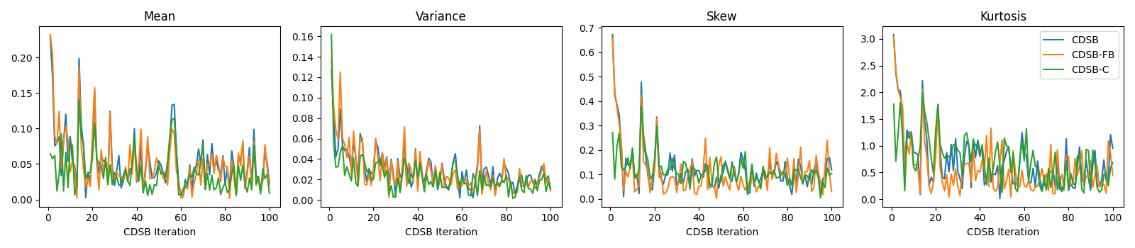
We report the estimated posterior moments as well as their standard deviation in Table 5. We further plot the convergence of RMSE for each of the statistics in Figure 7. As can be observed, IPF converges after about 20 iterations, and errors for all statistics are improved compared with CSGM (corresponding to IPF iteration 1). Using conditional initialization also helps with localizing the problem and reduces estimation errors especially in early iterations.

		MCMC	CDSB	CDSB-FB	CDSB-C	MGAN	IT
Mean	$x_{1}$	.075	.066±.010	.068±.010	.072±.007	.048	.034
	$x_{2}$	.875	.897±.019	.897±.017	.891±.013	.918	.902
Var	$x_{1}$	.190	.184±.007	.190±.007	.188±.005	.177	.206
	$x_{2}$	.397	.387±.006	.391±.006	.393±.005	.419	.457
Skew	$x_{1}$	1.94	1.90±.038	2.01±.041	1.90±.028	1.83	1.63
	$x_{2}$	.681	.591±.018	.628±.018	.596±.014	.630	.872
Kurt	$x_{1}$	8.54	7.85±.210	8.54±.239	8.00±.147	7.64	7.57
	$x_{2}$	3.44	3.33±.035	3.51±.041	3.27±.035	3.19	3.88

Table 5: Estimated posterior moments and their standard deviations for the BOD example. The closest estimates to MCMC are highlighted in bold.

Figure 7: Convergence of estimated posterior moments with increasing number of CDSB iterations.

G.4 Image Experiments

For all image experiments, we use the Adam optimizer with learning rate ${10}^{-4}$ and train for 500k iterations in total. Since both $\mathbf{F}$ and $\mathbf{B}$ needs to be trained, the training time is approximately doubled for CDSB. Following Song and Ermon [2020], we make use of the exponential moving average (EMA) of the network parameters with EMA rate 0.999 at test time. We use $\gamma_{\textup{min}}=5\times{10}^{-5}$ for all experiments unless indicated otherwise and perform a parameter sweep for $\gamma_{\textup{max}}$ in $\{0.005,0.01,0.05,0.1\}$. The optimal $\gamma_{\textup{max}}$ depends on the number of timesteps $N$ and the discrepancy between $p(x|y)$ and $p_{\textup{ref}}$. When using large $N$ or conditional $p_{\textup{ref}}(x|y)$, we find $\gamma_{\textup{max}}$ can be taken smaller.

G.4.1 MNIST

For the MNIST dataset, we use a U-Net architecture with 3 resolution levels each with 2 residual blocks. The numbers of filters at each resolution level are 64, 128, 128 respectively. The total number of parameters is 6.6m, and we use batch size 128 for training. Since we observe overfitting on the MNIST training set for all methods, we also apply dropout with $p=0.1$ for the MNIST experiments. For each CDSB iteration, 100k or 250k training steps are used, corresponding to $L=5$ or $L=2$ CDSB iterations in total, which we find to be sufficient on this simpler dataset.

For $N=10$, CDSB generates a minibatch of 100 images in approximately 0.8 seconds when run on a GTX 1080Ti. As a baseline comparison, we experimented with the methodology in Kadkhodaie and Simoncelli [2021] on the same MNIST test set and find that it gives PSNR/SSIM values of 15.78/0.72 and 12.49/0.47 for super-resolution and inpainting respectively (c.f. Table 2). Around 250 iterations are required for generating each image, or approximately 1 second generation time for 1 image on a GTX 1080Ti. In comparison, the CDSB methodology is much more efficient and achieves better image quality on both tasks.

(a) $y^{\textup{obs}}$

(b) Ground truth

(c) CSGM $N=5$

(d) CDSB $N=5$

(e) CDSB-C $N=5$

(f) CSGM $N=10$

(g) CDSB $N=10$

(h) CDSB-C $N=10$

Figure 8: Additional samples for the MNIST 4x SR task.

(a) CSGM $N=10$

(b) CDSB $N=10$

(c) CDSB-FB $N=10$

(d) CDSB-C $N=10$

Figure 9: Uncurated conditional samples for the MNIST 14x14 inpainting task. The first two columns correspond to ground truth, $y^{\textup{obs}}$, and the last two columns correspond to the mean and standard deviation of 100 samples.

G.4.2 CelebA 64x64

For the CelebA dataset, we use a U-Net architecture with 4 resolution levels each with 2 residual blocks and self-attention blocks at $16\times 16$ and $8\times 8$ resolutions. The numbers of filters at each resolution level are 128, 256, 256, 256 respectively. The total number of parameters is 39.6m, and we use batch size 128 for training. For each CDSB iteration, 10k or 25k training steps are used, corresponding to $L=50$ or $L=20$ CDSB iterations in total. For smaller $\gamma_{\textup{max}}$, we find that higher number of CDSB iterations are beneficial.

For $N=20,50$, CDSB generates a minibatch of 100 images in approximately 12, 30 seconds when run on a Titan RTX. As a baseline comparison, we find that CDSB-C with $N=20$ even outperforms a standard CSGM with $N=200$, which achieves PSNR/SSIM values of approximately 20.98/0.62. To ensure that conditional initialization is not the sole contributor to the gain in sample quality, we further compare CDSB-C ($N=50$) to a CSGM ($N=50$) with conditional initialization. The forward noising process is also modified to the discretized Ornstein–Uhlenbeck process targeting $p_{\textup{ref}}(x|y)$ as described in Section 5.2. This modification achieved PSNR/SSIM values of 20.84/0.59 (c.f. Table 2), which indicates that the CDSB framework presents larger benefits in addition to conditional initialization.

As another baseline comparison, the SNIPS algorithm [Kawar et al., 2021] reports PSNR of 21.90 for 8 CelebA test images and, when averaging across 8 predicted samples for each of the images, a PSNR of 24.31. The algorithm requires 2500 iterations for image generation, or approximately 2 minutes for producing 8 samples when run on an RTX 3080 as reported by Kawar et al. [2021]. On the same test benchmark, CDSB with $N=50$ achieved PSNR values of 21.87 and 24.20 respectively in 3.1 seconds, thus achieving similar levels of sample quality using much less iterations. Furthermore, the SNIPS algorithm is applicable specifically for tractable linear Gaussian inverse problems, whereas CDSB is more general and does not rely on tractable likelihoods.

G.4.3 CelebA 160x160

We adopt the official implementation and pre-trained checkpoints of SRFlow and make use of a higher resolution version of CelebA (160x160) following Lugmayr et al. [2020] in only Section 7.3.2. For CSGM and CDSB, we use a U-Net architecture with 4 resolution levels each with 2 residual blocks. The numbers of filters at each resolution level are 128, 256, 256, 512 respectively. The total number of parameters is 71.0m while SRFlow has total number of parameters 40.0m. We use a batch size of 32 for training the CSGM and CDSB models.

When $p_{\textup{ref}}(x|y)$ is defined by SRFlow, it is infeasible to use a discretized Ornstein–Uhlenbeck process targeting $p_{\textup{ref}}(x|y)$ as in Section 5.2. We instead use a discretized Brownian motion for $p_{k+1|k}$, or equivalently the Variance Exploding (VE) SDE [Song and Ermon, 2019, Song et al., 2021b]. This has the interpretation as a entropy regularized Wasserstein-2 optimal transport problem as discussed in Section 3.2, i.e. CDSB-C seeks to minimize the total squared transport distance between SRFlow $p_{\textup{ref}}(x|y)$ and the true posterior $p(x|y)$. We use the time schedule $\gamma_{\textup{min}}=\gamma_{\textup{max}}=0.005$ with comparatively higher $\gamma_{\textup{min}}$ in order to accelerate convergence under $N=10$ timesteps. We provide additional samples from SRFlow, CDSB-C as well as CSGM-C in Figures 13, 14, 15.

(a) $y^{\textup{obs}}$

(b) Ground truth

(c) CSGM $N=20$

(d) CDSB $N=20$

(e) CDSB-C $N=20$

(f) CSGM $N=50$

(g) CDSB $N=50$

(h) CDSB-C $N=50$

Figure 10: Uncurated samples for the CelebA 4x SR with Gaussian noise task.

(a) $y^{\textup{obs}}$

(b) Ground truth

(c) CSGM $N=20$

(d) CDSB $N=20$

(e) CDSB-C $N=20$

(f) CSGM $N=50$

(g) CDSB $N=50$

(h) CDSB-C $N=50$

Figure 11: Uncurated samples for the CelebA 4x SR with Gaussian noise task.

Figure 12: Uncurated conditional samples using CDSB-C with $N=50$ for the CelebA 4x SR with Gaussian noise task. The first two columns correspond to ground truth, $y^{\textup{obs}}$, and the last column corresponds to the mean of the middle 8 samples.

(a) $y^{\textup{obs}}$

(b) Ground truth

(c) SRFlow

(d) CSGM-C $N=10$

(e) CDSB-C $N=10$

Figure 13: Additional uncurated samples for the CelebA 8x SR task.

(a) $y^{\textup{obs}}$

(b) Ground truth

(c) SRFlow

(d) CSGM-C $N=10$

(e) CDSB-C $N=10$

Figure 14: Additional uncurated samples for the CelebA 8x SR task.

(a) $y^{\textup{obs}}$

(b) Ground truth

(c) SRFlow

(d) CSGM-C $N=10$

(e) CDSB-C $N=10$

Figure 15: Additional uncurated samples for the CelebA 8x SR task.

G.5 Optimal Filtering in State-Space Models

For the sake of completeness, we first give details of the Lorenz-63 model here. It is defined for $x\in\mathbb{R}^{3}$ under the following ODE system

$$\frac{\mathrm{d}x[1]}{\mathrm{d}\tau}=\sigma(x[2]-x[1]),\quad\frac{\mathrm{d}x[2]}{\mathrm{d}\tau}=x[1](\rho-x[3])-x[2],\quad\frac{\mathrm{d}x[3]}{\mathrm{d}\tau}=x[1]x[2]-\theta x[3].$$

We consider the values $\sigma=10$, $\rho=28$ and $\theta=8/3$, which results in chaotic dynamics famously known as the Lorenz attractor. We integrate this system using the 4th order Runge–Kutta method with step size 0.05. For the state-space model, we define $(X_{t})_{t\geq 1}$ as the states $(x[1],x[2],x[3])$ of the system at regular intervals of $\delta\tau=0.1$ with small Gaussian perturbations of mean 0 and variance ${10}^{-4}$, and $(Y_{t})_{t\geq 1}$ as noisy observations of $(X_{t})_{t\geq 1}$ with Gaussian noise of mean 0 and variance 4. More explicitly, the transition density is thus defined for $x_{t}=(x_{t}[1],x_{t}[2],x_{t}[3])\in\mathbb{R}^{3}$ as

$$f(x_{t}|x_{t-1})=\mathcal{N}(x_{t};\textup{RK4}(x_{t-1},0.1),{10}^{-4}\operatorname{Id}),\quad g(y_{t}|x_{t})=\mathcal{N}(y_{t};x_{t},4\operatorname{Id}),$$

where $\textup{RK4}(x_{t},0.1)$ is the 4th order Runge–Kutta operator (with step size 0.05) for the Lorenz-63 dynamics with initial condition $x_{t}$ and termination time 0.1.

We run the model for 4,000 time steps and perform Bayesian filtering for the last 2,000 time steps. To accelerate the sequential inference process, we use linear regression in this example to fit $\mathbf{F},\mathbf{B}$ with nonlinear feature expansion using radial basis functions. Similar to Spantini et al. [2022], we experiment with the number of nonlinear features from 1 to 3 RBFs, in addition to the linear feature. We find that as the ensemble size $M$ increases, increasing the number of features is helpful for lowering filtering errors, suggesting that bias-variance tradeoff is at play.

Since the system’s dynamics are chaotic and can move far from the origin and display different scaling for each dimension, it is not suitable to choose $p_{\textup{ref}}(x)=\mathcal{N}(x;0,\operatorname{Id})$. Therefore, for CSGM and CDSB, we let $p_{\textup{ref}}(x)=\mathcal{N}(x;\mu_{\textup{ref}},\textup{diag}(\sigma_{\textup{ref}}^{2}))$ where $\mu_{\textup{ref}},\sigma_{\textup{ref}}^{2}$ are the estimated mean and variance of the prior predictive distribution $p(x_{t}|y^{\textup{obs}}_{1:t-1})$ at time $t$. For CSGM-C and CDSB-C, we let $p_{\textup{ref}}(x|y)=\mathcal{N}(x;\mu_{\textup{ref}},\textup{diag}(\sigma_{\textup{ref}}^{2}))$ where the estimated posterior mean and variance are returned by EnKF. Furthermore, we scale the diffusion process’s time step dimensionwise by the variance of the reference measure $\sigma_{\textup{ref}}^{2}$. We consider a short diffusion process with $N=20$, and a long diffusion process with $N=100$. We let $\gamma_{\textup{min}}=0.0005\cdot\sigma_{\textup{ref}}^{2}$ and $\gamma_{\textup{max}}=0.05\cdot\sigma_{\textup{ref}}^{2}$ for the short diffusion process, and reduce $\gamma_{\textup{max}}$ by a half for the long diffusion process.

We report the RMSEs between each algorithm’s filtering means and the ground truth filtering means in Table 4. We compute the ground truth filtering means using a particle filter with $M={10}^{6}$ particles. In addition, we report the RMSEs between each algorithm’s filtering means and the true states $x_{1:T}$ in Table 6a, and between each algorithm’s filtering standard deviations and the ground truth standard deviations in Table 6b. Similarly, we observe that CDSB and CDSB-C achieve lower errors than CSGM and EnKF. Interestingly, CSGM-C performs similarly well as CDSB-C for state estimation when $N=100$ steps, but performs worse for standard deviation estimation. In the case where the ensemble size $M=200$, however, when using the long diffusion process we observe occasional large errors for CDSB and CDSB-C. We conjecture that since CDSB is an iterative algorithm, inevitably small errors in regression can be accumulated. For small ensemble size and large number of diffusion steps, the model may thus be more prone to overfitting. However, for larger ensemble size $M\geq 500$ we do not observe this issue.

$M$	200	500	1000	2000
EnKF	.476±.010	.474±.005	.475±.005	.475±.003
CSGM (short)	Diverges
CDSB (short)	.464±.013	.391±.010	.369±.007	.352±.008
CSGM-C (short)	Diverges
CDSB-C (short)	.428±.016	.378±.012	.359±.015	.340±.007
CSGM (long)	.431±.010	.376±.008	.360±.012	.343±.006
CDSB (long)	.582±.328	.370±.012	.348±.006	.333±.006
CSGM-C (long)	.434±.057	.367±.011	.346±.008	.336±.004
CDSB-C (long)	.660±.310	.368±.016	.344±.010	.331±.006

(a)

$M$	200	500	1000	2000
EnKF	.255±.003	.286±.002	.296±.001	.300±.003
CSGM (short)	Diverges
CDSB (short)	.203±.005	.167±.003	.150±.002	.137±.002
CSGM-C (short)	Diverges
CDSB-C (short)	.148±.004	.124±.002	.108±.002	.099±.001
CSGM (long)	.204±.005	.163±.008	.140±.002	.129±.001
CDSB (long)	.140±.008	.129±.003	.123±.003	.120±.002
CSGM-C (long)	.186±.005	.142±.003	.120±.001	.109±.002
CDSB-C (long)	.176±.006	.120±.002	.110±.003	.106±.002

(b)

Table 6: RMSEs over 10 runs between (a) each algorithm’s filtering means and the true states $x_{1:T}$ for $N=20$ (short) and $N=100$ (long); (b) each algorithm’s filtering standard deviations and the ground truth filtering standard deviations. The lowest errors are highlighted in bold.

References

• Baptista et al. [2020] Ricardo Baptista, Olivier Zahm, and Youssef Marzouk. An adaptive transport framework for joint and conditional density estimation. arXiv preprint arXiv:2009.10303, 2020.
• Batzolis et al. [2021] Georgios Batzolis, Jan Stanczuk, Carola-Bibiane Schönlieb, and Christian Etmann. Conditional image generation with score-based diffusion models. arXiv preprint arXiv:2111.13606, 2021.
• Beaumont [2019] Mark A Beaumont. Approximate Bayesian computation. Annual Review of Statistics and Its Applications, 6:379–403, 2019.
• Bernton et al. [2019] Espen Bernton, Jeremy Heng, Arnaud Doucet, and Pierre E Jacob. Schrödinger bridge samplers. arXiv preprint arXiv:1912.13170, 2019.
• Cattiaux et al. [2021] Patrick Cattiaux, Giovanni Conforti, Ivan Gentil, and Christian Léonard. Time reversal of diffusion processes under a finite entropy condition. arXiv preprint arXiv:2104.07708, 2021.
• Chen et al. [2021a] Nanxin Chen, Yu Zhang, Heiga Zen, Ron J Weiss, Mohammad Norouzi, and William Chan. Wavegrad: Estimating gradients for waveform generation. In International Conference on Learning Representations, 2021a.
• Chen et al. [2022] Tianrong Chen, Guan-Horng Liu, and Evangelos A Theodorou. Likelihood training of Schrödinger bridge using forward-backward SDEs theory. In International Conference on Learning Representations, 2022.
• Chen et al. [2021b] Yongxin Chen, Tryphon T Georgiou, and Michele Pavon. Optimal transport in systems and control. Annual Review of Control, Robotics, and Autonomous Systems, 4, 2021b.
• Choi et al. [2021] Jooyoung Choi, Sungwon Kim, Yonghyun Jeong, Youngjune Gwon, and Sungroh Yoon. Ilvr: Conditioning method for denoising diffusion probabilistic models. arXiv preprint arXiv:2108.02938, 2021.
• Chung et al. [2021] Hyungjin Chung, Byeongsu Sim, and Jong Chul Ye. Come-closer-diffuse-faster: Accelerating conditional diffusion models for inverse problems through stochastic contraction. arXiv preprint arXiv:2112.05146, 2021.
• De Bortoli et al. [2021] Valentin De Bortoli, James Thornton, Jeremy Heng, and Arnaud Doucet. Diffusion Schrödinger bridge with applications to score-based generative modeling. In Advances in Neural Information Processing Systems, 2021.
• Dhariwal and Nichol [2021] Prafulla Dhariwal and Alex Nichol. Diffusion models beat GAN on image synthesis. In Advances in Neural Information Processing Systems, 2021.
• Dockhorn et al. [2022] Tim Dockhorn, Arash Vahdat, and Karsten Kreis. Score-based generative modeling with critically-damped Langevin diffusion. In International Conference on Learning Representations, 2022.
• Doucet and Johansen [2009] Arnaud Doucet and Adam M Johansen. A tutorial on particle filtering and smoothing: Fifteen years later. Handbook of Nonlinear Filtering, 12(656-704):3, 2009.
• Durmus and Moulines [2017] Alain Durmus and Éric Moulines. Nonasymptotic convergence analysis for the unadjusted Langevin algorithm. The Annals of Applied Probability, 27(3):1551–1587, 2017.
• Ho and Salimans [2021] Jonathan Ho and Tim Salimans. Classifier-free diffusion guidance. In NeurIPS 2021 Workshop on Deep Generative Models and Downstream Applications, 2021.
• Ho et al. [2020] Jonathan Ho, Ajay Jain, and Pieter Abbeel. Denoising diffusion probabilistic models. In Advances in Neural Information Processing Systems, 2020.
• Hyvärinen [2005] Aapo Hyvärinen. Estimation of non-normalized statistical models by score matching. Journal of Machine Learning Research, 6(4), 2005.
• Jolicoeur-Martineau et al. [2021] Alexia Jolicoeur-Martineau, Ke Li, Rémi Piché-Taillefer, Tal Kachman, and Ioannis Mitliagkas. Gotta go fast when generating data with score-based models. arXiv preprint arXiv:2105.14080, 2021.
• Kadkhodaie and Simoncelli [2021] Zahra Kadkhodaie and Eero P Simoncelli. Stochastic solutions for linear inverse problems using the prior implicit in a denoiser. In Advances in Neural Information Processing Systems, 2021.
• Kawar et al. [2021] Bahjat Kawar, Gregory Vaksman, and Michael Elad. SNIPS: Solving noisy inverse problems stochastically. In Advances in Neural Information Processing Systems, 2021.
• Kawar et al. [2022] Bahjat Kawar, Michael Elad, Stefano Ermon, and Jiaming Song. Denoising diffusion restoration models. arXiv preprint arXiv:2201.11793, 2022.
• Kingma et al. [2021] Diederik P Kingma, Tim Salimans, Ben Poole, and Jonathan Ho. Variational diffusion models. In Advances in Neural Information Processing Systems, 2021.
• Kovachki et al. [2021] Nikola Kovachki, Ricardo Baptista, Bamdad Hosseini, and Youssef Marzouk. Conditional sampling with monotone GANs. arXiv preprint arXiv:2006.06755, 2021.
• Kruse et al. [2021] Jakob Kruse, Gianluca Detommaso, Ullrich Köthe, and Robert Scheichl. HINT: Hierarchical invertible neural transport for density estimation and Bayesian inference. In AAAI Conference on Artificial Intelligence, 2021.
• Kullback [1968] Solomon Kullback. Probability densities with given marginals. The Annals of Mathematical Statistics, 39(4):1236–1243, 1968.
• Kullback [1997] Solomon Kullback. Information Theory and Statistics. Dover Publications, Inc., Mineola, NY, 1997. Reprint of the second (1968) edition.
• Law et al. [2015] Kody Law, Andrew Stuart, and Kostantinos Zygalakis. Data Assimilation. Springer, 2015.
• Léger [2021] Flavien Léger. A gradient descent perspective on Sinkhorn. Applied Mathematics & Optimization, 84(2):1843–1855, 2021.
• Léonard [2014] Christian Léonard. Some properties of path measures. In Séminaire de Probabilités XLVI, pages 207–230. Springer, 2014.
• Li et al. [2022] Haoying Li, Yifan Yang, Meng Chang, Shiqi Chen, Huajun Feng, Zhihai Xu, Qi Li, and Yueting Chen. Srdiff: Single image super-resolution with diffusion probabilistic models. Neurocomputing, 479:47–59, 2022.
• Lu et al. [2022] Yen-Ju Lu, Zhong-Qiu Wang, Shinji Watanabe, Alexander Richard, Cheng Yu, and Yu Tsao. Conditional diffusion probabilistic model for speech enhancement. In ICASSP 2022 - 2022 IEEE International Conference on Acoustics, Speech and Signal Processing (ICASSP), 2022.
• Lugmayr et al. [2020] Andreas Lugmayr, Martin Danelljan, Luc Van Gool, and Radu Timofte. Srflow: Learning the super-resolution space with normalizing flow. In ECCV, 2020.
• Luhman and Luhman [2021] Eric Luhman and Troy Luhman. Knowledge distillation in iterative generative models for improved sampling speed. arXiv preprint arXiv:2101.02388, 2021.
• Marzouk et al. [2016] Youssef Marzouk, Tarek Moselhy, Matthew Parno, and Alessio Spantini. Sampling via measure transport: An introduction. Handbook of Uncertainty Quantification, pages 1–41, 2016.
• Meng et al. [2022] Chenlin Meng, Yutong He, Yang Song, Jiaming Song, Jiajun Wu, Jun-Yan Zhu, and Stefano Ermon. SDEdit: Guided image synthesis and editing with stochastic differential equations. In International Conference on Learning Representations, 2022.
• Peyré and Cuturi [2019] Gabriel Peyré and Marco Cuturi. Computational optimal transport. Foundations and Trends® in Machine Learning, 11(5-6):355–607, 2019.
• Reich [2019] Sebastian Reich. Data assimilation: the Schrödinger perspective. Acta Numerica, 28:635–711, 2019.
• Saharia et al. [2021] Chitwan Saharia, Jonathan Ho, William Chan, Tim Salimans, David J Fleet, and Mohammad Norouzi. Image super-resolution via iterative refinement. arXiv preprint arXiv:2104.07636, 2021.
• Salimans and Ho [2022] Tim Salimans and Jonathan Ho. Progressive distillation for fast sampling of diffusion models. In International Conference on Learning Representations, 2022.
• Song et al. [2021a] Jiaming Song, Chenlin Meng, and Stefano Ermon. Denoising diffusion implicit models. In International Conference on Learning Representations, 2021a.
• Song and Ermon [2019] Yang Song and Stefano Ermon. Generative modeling by estimating gradients of the data distribution. In Advances in Neural Information Processing Systems, 2019.
• Song and Ermon [2020] Yang Song and Stefano Ermon. Improved techniques for training score-based generative models. In Advances in Neural Information Processing Systems, 2020.
• Song et al. [2021b] Yang Song, Jascha Sohl-Dickstein, Diederik P. Kingma, Abhishek Kumar, Stefano Ermon, and Ben Poole. Score-based generative modeling through stochastic differential equations. In International Conference on Learning Representations, 2021b.
• Spantini et al. [2022] Alessio Spantini, Ricardo Baptista, and Youssef Marzouk. Coupling techniques for nonlinear ensemble filtering. SIAM Review, 2022. to appear.
• Taghvaei and Hosseini [2022] Amirhossein Taghvaei and Bamdad Hosseini. An optimal transport formulation of Bayes’ law for nonlinear filtering algorithms. arXiv preprint arXiv:2203.11869, 2022.
• Tashiro et al. [2021] Yusuke Tashiro, Jiaming Song, Yang Song, and Stefano Ermon. CSDI: Conditional score-based diffusion models for probabilistic time series imputation. In Advances in Neural Information Processing Systems, 2021.
• Vargas et al. [2021] Francisco Vargas, Pierre Thodoroff, Austen Lamacraft, and Neil Lawrence. Solving Schrödinger bridges via maximum likelihood. Entropy, 23(9):1134, 2021.
• Vincent [2011] Pascal Vincent. A connection between score matching and denoising autoencoders. Neural Computation, 23(7):1661–1674, 2011.
• Watson et al. [2022] Daniel Watson, William Chan, Jonathan Ho, and Mohammad Norouzi. Learning fast samplers for diffusion models by differentiating through sample quality. arXiv preprint arXiv:2202.05830, 2022.
• Xiao et al. [2021] Zhisheng Xiao, Karsten Kreis, and Arash Vahdat. Tackling the generative learning trilemma with denoising diffusion GANs. arXiv preprint arXiv:2112.07804, 2021.
• Zheng et al. [2022] Huangjie Zheng, Pengcheng He, Weizhu Chen, and Mingyuan Zhou. Truncated diffusion probabilistic models. arXiv preprint arXiv:2202.09671, 2022.
• Zhou et al. [2022] Xingyu Zhou, Yuling Jiao, Jin Liu, and Jian Huang. A deep generative approach to conditional sampling. Journal of the American Statistical Association, 2022. to appear.