Neural-Progressive Hedging: Enforcing Constraints in Reinforcement Learning with Stochastic Programming

Abstract

We propose a framework, called neural-progressive hedging (NP), that leverages stochastic programming during the online phase of executing a reinforcement learning (RL) policy. The goal is to ensure feasibility with respect to constraints and risk-based objectives such as conditional value-at-risk (CVaR) during the execution of the policy, using probabilistic models of the state transitions to guide policy adjustments. The framework is particularly amenable to the class of sequential resource allocation problems since feasibility with respect to typical resource constraints cannot be enforced in a scalable manner. The NP framework provides an alternative that adds modest overhead during the online phase. Experimental results demonstrate the efficacy of the NP framework on two continuous real-world tasks: (i) the portfolio optimization problem with liquidity constraints for financial planning, characterized by non-stationary state distributions; and (ii) the dynamic repositioning problem in bike sharing systems, that embodies the class of supply-demand matching problems. We show that the NP framework produces policies that are better than deep RL and other baseline approaches, adapting to non-stationarity, whilst satisfying structural constraints and accommodating risk measures in the resulting policies. Additional benefits of the NP framework are ease of implementation and better explainability of the policies.

1 Introduction

Reinforcement learning (RL) experienced a surge in popularity when deep models demonstrated superior performance in game playing with Deep Q-learning Networks (DQN) [Mnih et al., 2013]. The role of RL was cemented when it was used to beat the reigning Go world champion [Silver et al., 2017]. Improvements to deep RL algorithms have abounded, including RL for continuous state and action spaces, with DDPG [Lillicrap et al., 2015], TRPO [Schulman et al., 2015], and PPO [Schulman et al., 2017]. In spite of these advances, the dominance of RL for real-world problems has lagged. We believe that this is due to three shortcomings.

First, RL policies cannot enforce business rules, or constraints during policy execution. Yet, often structural constraints must be respected for a policy to be implementable. Existing methods, such as constrained policy gradient [Achiam et al., 2017] or “safe" RL methods [Garcıa and Fernández, 2015] do not prevent constraint violations during policy execution. Moreover, these methods can often be difficult to train and not scalable to large problems. Second, there is a natural trade-off between expected reward and risk. The majority of RL algorithms seek to maximize the expected return. While there have been RL algorithms that optimize for various risk measures, doing so in a scalable manner and under constraints is still challenging. Third, the sample inefficiency of RL has posed an impediment to solving problems where high-fidelity simulators are not available to generate sufficiently large number of sample trajectories. A hope to overcoming this is through the judicious use of models to explore more sparingly the state and action spaces.

We introduce a framework to address these issues for problems with continuous state and action spaces. An unconstrained RL policy is first trained offline. During the online execution phase, a stochastic program (SP) is used to re-optimize the given RL policy under constraints and risk measures over a short-term future trajectory. Once the next action is chosen, the process repeats in a rolling-horizon fashion using updated state information. We call this neural-progressive hedging (NP). The NP method aims to exploit the generalization ability of RL to unseen scenarios jointly with the ability of SP to exploit models and enforce scenario-dependent constraints as well as incorporating risk measures. Since the NP framework relies on a model-based online phase, it is most useful in problem settings where closed-form models of state transitions are relatively good approximations to the true state transitions. Sequential and dynamic resource allocation problems are a key example in which the NP framework excels.

Empirically, we show that the NP method results in policies that offer substantial improvements in reward under various risk measures whilst satisfying hard constraints. Moreover, we observe that the NP policy, with its more sample-efficient initial RL policy followed by the online fine-tuning phase, is able to outperform the fully-trained (and data-hungry) RL policy. An additional benefit of the framework is ease of implementation: it can be implemented using existing deep RL algorithms and off-the-shelf optimization packages. To that end, the key contributions of the paper are as follows:

1. We define a novel method, neural-progressive hedging, combining stochastic programming model-based online planning with offline, deep RL for a continuous policy that satisfies hard constraints during execution;

2. We incorporate risk-measures such as CVaR without sacrificing model structure or decomposition algorithm; and

3. We demonstrate the efficacy of the NP method on the class of resource allocation models, including two real-world problems: (i) liquidity-constrained portfolio optimization with a CVaR objective; and (ii) dynamic repositioning in a bike sharing system, where the NP method outperforms deep RL, both constrained and unconstrained as well as other baselines.

2 Preliminaries

Consider the problem of learning a deterministic policy $\pi:\mathcal{S}\rightarrow\mathcal{A}$ in a Markov Decision Process (MDP) given by $(\mathcal{S},\mathcal{A},p,f,\gamma,T,G)$, with continuous states $s\in\mathcal{S}$, continuous actions $x\in\mathcal{A}$, transition probability distribution $p(s_{t+1}|s_{t},x_{t})$, cost function $f(s_{t},x_{t},s_{t+1})\in\mathbb{R}$, discount factor $\gamma\in[0,1]$, decision horizon $T$, and constraint set $G$. We allow $T=\infty$ whenever $\gamma<1$. The constraint set $G$ contains a set of $K$ additional cost functions $g_{1}\ldots g_{K}$ where $g_{k}(s_{t},x_{t},s_{t+1})\in\mathbb{R}$ and constants $\beta_{1}\ldots\beta_{K}\in\mathbb{R}$. Our constrained MDP setting follows that of Altman [1999], where we aim to solve the following problem:

$$\underset{\pi}{\text{minimize }} \mathbb{E}_{\pi}\left[\sum_{t=1}^{T}\gamma^{t-1}f(s_{t},x_{t},s_{t+1})\right]$$ (1)

s.t. $$\mathbb{E}_{\pi}\left[\sum_{t=1}^{T}\gamma^{t-1}g_{k}(s_{t},x_{t},s_{t+1})\right]\!\!\leq\beta_{k},\quad k\!=\!1\ldots K.$$

Without loss of generality we assume a fixed initial state $s_{1}$. The expectation $\mathbb{E}_{\pi}$ is taken with respect to randomness induced by the transitions $s_{t+1}\sim p(\cdot|s_{t},x_{t})$ by taking $x_{t}=\pi(s_{t})$, for all $t$. Problem (1) is very challenging to solve for general MDPs with continuous states and actions. We shall now put this constrained MDP in the context of stochastic programming (SP) from which we borrow many of the algorithmic tools in this work.

The key assumption from SP is that all the randomness or uncertainty in the system comes from external sources. This decoupling of randomness allows us to employ powerful optimization tools in solving the main problem. Assume $T$ is finite and let $\xi_{1}\ldots\xi_{T}$ be random variables such that the next state $s_{t+1}$ is given by $s_{t+1}=\tilde{p}(s_{t},x_{t},\xi_{t})$ where $\tilde{p}$ is a deterministic function once $\xi_{t}$ is fixed. We call each realization of $\xi=(\xi_{1}\ldots\xi_{T})$ a scenario. Given a particular scenario $\xi$ , one can find the best action sequence in “hindsight” by solving the following problem:

$$\underset{x=(x_{1}\ldots x_{T})}{\text{minimize}}\quad \tilde{f}(x,\xi)$$ (2)

s.t. $$\tilde{g}_{k}(x,\xi)\leq\beta_{k},\quad k=1\ldots K$$

where we define

$$\tilde{f}(x,\xi):=\sum_{t=1}^{T}\gamma^{t-1}f[s_{t},x_{t},\tilde{p}(s_{t},x_{t},\xi_{t})]\hskip 13.00806pt$$

$$\tilde{g}_{k}(x,\xi):=\sum_{t=1}^{T}\gamma^{t-1}g_{k}[s_{t},x_{t},\tilde{p}(s_{t},x_{t},\xi_{t})].$$

If, for each $\xi$, the functions $\tilde{f}$ and $\tilde{g}_{k}$ for all $k$ are all convex in $x$, then each scenario sub-problem can be readily solved using existing convex optimization tools. To simplify notation, we define the constraint set $\mathcal{G}(\xi):=\{x|\tilde{g}_{k}(x,\xi)\leq\beta_{k},k=1\ldots K\}$, so problem  (2) can be stated simply as $\text{minimize}_{x\in\mathcal{G}(\xi)}\tilde{f}(x,\xi)$.

Suppose that one starts with a finite set $\Xi$ of scenarios, with known probability distribution $q(\xi)$ where $\sum_{\xi\in\Xi}q(\xi)=1$. One can solve problem (2) for each individual $\xi\in\Xi$ to obtain a mapping $x(\cdot)$ that provides a solution $x(\xi)=(x_{1}(\xi)\ldots x_{T}(\xi))$ for each $\xi\in\Xi$. Suppose that the action space $\mathcal{A}\subseteq\mathbb{R}^{n}$ and $|\Xi|=N$, then $x(\cdot)\in\mathcal{A}^{N\times T}\subseteq\mathbb{R}^{N\times T\times n}$. How could we then reconcile the various $x_{t}(\xi)$ across all $\xi\in\Xi$, at time $t$? For the resulting solutions to be implementable, one needs to enforce a nonanticipative property which states that $x_{t}$ must only depend on information available at time $t$. From an MDP point of view, the state $s_{t}$ captures all observations available up to time $t$, represented by $\xi_{1}\ldots\xi_{t-1}$, and therefore $x_{t}$ must only depend on these if it is to be implementable, i.e., $x_{t}(\xi)=x_{t}(\xi_{1},\ldots,\xi_{t-1})$ and $x_{1}(\xi)$ must be the same for all $\xi$. All solutions $x(\cdot)$ that satisfy this nonanticipative property can be expressed as:

$$x(\xi)=(x_{1},x_{2}(\xi_{1}),\ldots,x_{T}(\xi_{1},\ldots,\xi_{T-1})),\quad\forall\xi\in\Xi.$$

We use $\mathcal{M}$ to denote the space of all nonanticipative mappings. Define an inner product on $\mathcal{A}^{N\times T}$ by $\langle x(\cdot),w(\cdot)\rangle:=\sum_{\xi}q(\xi)\sum_{t=1}^{T}\langle x_{t}(\xi),w_{t}(\xi)\rangle$ where $\langle x_{t}(\xi),w_{t}(\xi)\rangle$ is the standard inner product in $\mathbb{R}^{n}$. Given any $\hat{x}(\cdot)\in\mathcal{A}^{N\times T}$, one can find a nonanticipative version $x(\cdot)=P_{\mathcal{M}}[\hat{x}(\cdot)]$ where $P_{\mathcal{M}}$ is the orthogonal projection onto $\mathcal{M}$ given by the conditional expectation $x_{t}(\xi)=\mathbb{E}_{\xi|\xi_{1}\ldots\xi_{t-1}}\hat{x}_{t}(\xi)$ for all $t$ and $\xi$. Note that $P_{\mathcal{M}}$ can be computed via simple averaging over the appropriate subsets of scenarios.

Define $\mathcal{G}\subseteq\mathcal{A}^{N\times T}$ such that $x(\cdot)\in\mathcal{G}$ iff $x(\xi)\in\mathcal{G}(\xi)$ for all $\xi$. We then aim to solve the following global problem:

$$\underset{x(\cdot)\in\mathcal{G}\cap\mathcal{M}}{\text{minimize}}\quad\mathbb{E}_{\xi}\tilde{f}(x(\xi),\xi)$$ (3)

where $\mathbb{E}_{\xi}\tilde{f}(x(\xi),\xi)=\sum_{\xi\in\Xi}q(\xi)\tilde{f}(x(\xi),\xi)$. Without the constraint $x(\cdot)\in\mathcal{M}$, problem (3) would in fact be separable and could be decomposed into solving individual scenarios as in problem (2). This problem, however, can still be solved in an iterative manner where each iteration involves solving a slightly modified version of problem (2) for each scenario. This “progressive hedging” algorithm by Rockafellar and Wets [1991], which is an application of the proximal point algorithm, involves keeping track of the solution $x^{i}(\cdot)$ as well as a Lagrange multiplier $\lambda^{i}(\cdot)$ in each iteration $i$, until convergence. It also involves a parameter $\nu^{i}>0$, which may be constant for all $i$. Each iteration involves solving the following steps:

1. At iteration $i$, solve the following for each scenario $\xi$:

   $$\hat{x}^{i}(\xi)\in\arg\min_{x(\xi)\in\mathcal{G}(\xi)}\tilde{f}(x(\xi),\xi)+\langle\lambda^{i}(\xi),x(\xi)\rangle+\frac{\nu^{i}}{2}\|x(\xi)-x^{i}(\xi)\|^{2}$$ (4)

2. Compute $x^{i+1}(\cdot)=P_{\mathcal{M}}[\hat{x}^{i}(\cdot)]$.

3. Update the Lagrange multiplier $\lambda^{i+1}(\cdot)=\lambda^{i}(\cdot)+\nu^{i}[\hat{x}^{i}(\cdot)-x^{i+1}(\cdot)]$.

In the case where $\tilde{f}$ and $\mathcal{G}$ are both convex, the algorithm is guaranteed to converge to an optimal solution $x^{*}(\cdot)$ of problem (3) starting from arbitrary $x^{1}(\cdot)$ and $\lambda^{1}(\cdot)$. Local convergence to a stationary point for nonconvex $\tilde{f}$ was shown by Rockafellar [2019].

The SP framework can be adapted to measures of risk. Consider CVaR, the conditional value-at-risk, a popular measure for finding risk-averse solutions. The CVaR of a random variable $Z$ at level $\alpha\in[0,1)$ can be written as:

$$\mathrm{CVaR}_{\alpha}(Z):=\min_{y\in\mathbb{R}}\left\{y+\frac{1}{1-\alpha}\mathbb{E}_{Z}\left[\max\{0,Z-y\}\right]\right\}.$$

CVaR at $\alpha=0$ gives the expectation. We solve the CVaR version of problem (3), replacing the expectation $\mathbb{E}_{\xi}$ with $\mathrm{CVaR}_{\alpha}$, by following a modified progressive hedging algorithm [Rockafellar, 2018] with an introduction of an additional variable $y^{i}(\xi)\in\mathbb{R}$ and the corresponding dual $u^{i}(\xi)\in\mathbb{R}$ for each $\xi$. Instead of equation (4), we solve equation  (5) in step 1 with corresponding changes in steps 2 and 3.

$$(\hat{y}^{i}(\xi),\hat{x}^{i}(\xi))\in \arg\min_{y(\xi)\in\mathbb{R},x(\xi)\in\mathcal{G}(\xi)}\Big{\{}y(\xi)+\frac{1}{1-\alpha}\cdot\max\{0,\tilde{f}(x(\xi),\xi)-y(\xi)\}+$$

$$\frac{\nu^{i}}{2}|y(\xi)-y^{i}(\xi)|^{2}+u^{i}(\xi)y(\xi)+\langle\lambda^{i}(\xi),x(\xi)\rangle+\frac{\nu^{i}}{2}\|x(\xi)-x^{i}(\xi)\|^{2}\Big{\}}$$ (5)

3 Neural-Progressive Hedging

We introduce Neural-Progressive Hedging (NP) method combining the generalization capability of offline RL with the ability of SP through an online phase to exploit models while enforcing scenario-dependent constraints and risk measures. The key steps of the NP method are shown compactly in Algorithm 1.

The NP method works as follows: an unconstrained RL policy $\pi_{\theta}$, parameterized by $\theta$, is obtained by solving (1), or its risk-aware counterpart, without constraints. In each time-step $\tau$, the NP method observes current state $s_{(\tau)}$ and queries RL policy $\pi_{\theta}$ to get initial action $x^{\pi}(\cdot)$. The new NP policy is guided by the initial RL policy via a convex combination parameter $\kappa$ so that, at convergence, the executed actions satisfy constraints of $\mathcal{G}$ and the risk measures. Inner iterations are denoted by $i=1,\ldots$; at each iteration $i$, the SP sub-problems are solved for each scenario $\xi\in\Xi$ with updated Lagrangian multipliers $\lambda^{i},u^{i}$ to obtain the dual solution $\hat{x}^{i}(\xi)$ and $\hat{y}^{i}(\xi)$. Then, we project $\hat{x}^{i}(\xi)$ onto a feasible space $P_{\mathcal{M}}[\hat{x}^{i}(\cdot)]$, that satisfies the nonanticipative property, by averaging over all the scenarios. The primal solution $x^{i+1}(\cdot)$ is obtained as a convex combination with the initial RL policy $x^{\pi}(\cdot)$ then projected with $P_{\mathcal{M}}[\hat{x}^{i}(\cdot)]$. We then update multipliers $\lambda^{i},u^{i}$, and parameters $\kappa^{i}$, and $\nu^{i}$. This iterative process continues until the difference between primal and dual solutions, $\delta^{i}$, is below a pre-defined threshold $\epsilon$.

Algorithm 1 Neural-Progressive Hedging Algorithm

  Initialization: Obtain RL policy $\pi_{\theta}$. Define inner convergence criterion $\epsilon$, convex combination parameters $\kappa^{i}$ and penalty parameters $\nu^{i}>0$ for $i>0$.

  for $\tau=1,2,\ldots$,  do

     Observe state $s_{(\tau)}$. Sample scenario set $\Xi$, and query $\pi_{\theta}$ to obtain $x^{\pi}(\cdot)$. Set $x^{1}(\cdot)=x^{\pi}(\cdot)$. Set $\lambda^{1}(\cdot)=0$, $u^{1}(\cdot)=0$ and $i=1$.

     while  convergence criterion $\delta^{i}>\epsilon$  do

        1. Solve, for each $\xi\in\Xi$, (5) (or (4) for the risk-neutral case) to obtain $\hat{x}^{i}(\xi)$ and $\hat{y}^{i}(\xi)$.

        2. Set $x^{i+1}(\cdot)=\kappa^{i}x^{\pi}(\cdot)+(1-\kappa^{i})P_{\mathcal{M}}[\hat{x}^{i}(\cdot)]$. Set ${y}^{i+1}(\cdot)=\mathbb{E}_{\xi}[\hat{y}^{i}(\cdot)].$

        3. Update multipliers: $\lambda^{i+1}(\cdot)=\lambda^{i}(\cdot)+\nu^{i}(\hat{x}^{i}(\cdot)-x^{i+1}(\cdot))$ and $u^{i+1}(\cdot)=u^{i}(\cdot)+\nu^{i}(\hat{y}^{i}(\cdot)-y^{i+1}(\cdot)).$

        4. Update $\kappa^{i}$, $\nu^{i}$.

        5. Convergence test: $\delta^{i+1}:=\|\hat{x}^{i}(\cdot)-x^{i}(\cdot)\|+\|\hat{y}^{i}(\cdot)-y^{i}(\cdot)\|$

        6. Set $i\leftarrow i+1$, continue.

     end while

     From converged solution $x^{*}(\cdot)$, obtain and execute $x^{*}_{1}$.

  end for

Resource Allocation Problems:

The NP approach is particularly effective for the class of resource allocation problems. In such applications, the main source of uncertainty is external – consider stock price changes or customer demands – and to a large extent such random variables are unaffected by the actions of the policy. A scenario generator can hence be readily trained using historical data. The set of scenarios, $\Xi$, is obtained by sampling from such a scenario generator. Given a scenario, $\xi$, this policy can then be queried at any state $s_{t}$ to obtain the corresponding action $x_{t}$. Given a finite scenario set $\Xi$, we can obtain from $\pi_{\theta}$ its solution $x^{\pi}(\cdot)\in\mathcal{M}$.

3.1 Theoretical Analysis

The parameter $\kappa^{i}$ blends the offline RL policy with the solution from SP (Step 2 in Algorithm 1). The assumption below covers the settings of warm start, where $\kappa^{1}=1$ and $\hat{\imath}=2$, and imitation learning, where $\kappa^{i}$ is a decreasing sequence such as $(1+i)^{-2}$, where $1\leq\hat{\imath}<\infty$.

Assumption 1 (Imitation learning and warm start)

Let $\kappa^{i}\rightarrow 0$ as $i\rightarrow\infty$. Furthermore, there exists an $\hat{\imath}$ such that for all $i\geq\hat{\imath}$, $\kappa^{i}=0$.

Assumption 2 (Existence and local convexity)

Assume that the solution set of equation (5) for a CVaR objective, or equation (4) otherwise, is nonempty and finite, $\mathcal{G}(\xi)$ is convex and compact, the gradients of $\tilde{f}$ are locally Lipschitz for each $\xi$ and that the dual penalty parameters $\nu^{i}$ are sufficiently large for all $i$.

Lemma 1

Under Assumption 1, the NP algorithm is equivalent to the progressive hedging algorithm over an infinite number of iterations.

Proof: Assumption 1 states that there exists a finite iterate $\hat{\imath}$ such that for all $i\geq\hat{\imath}$, $\kappa^{i}=0$. Since $x^{i+1}(\cdot)=\kappa^{i}x^{\pi}(\cdot)+(1-\kappa^{i})P_{\mathcal{M}}[\hat{x}^{i}(\cdot)]$, for all $i^{\prime}\geq\hat{\imath}$, $x^{i^{\prime}}(\cdot)=P_{\mathcal{M}}[\hat{x}^{i^{\prime}}(\cdot)]$, and hence the update of the primal variable of the algorithm reduces to the progressive hedging update. $\blacksquare$

Instances of stochastic programming typically make use of discretized support $\Xi$. We thus define the problem (3) in terms of a discrete $\Xi$ and refer to this problem for the remainder of this section.

Assumption 3 (Discrete support)

Let $\Xi$ be a discrete support and let $1\ldots K$ index each scenario corresponding to a random variable $\xi\in\Xi$, with probability $p_{k}=1/K$. Then, problem (3) can be expressed as:

$$\min_{x_{k}\in{\cal G}_{k};x_{k}\in{\cal M}}\frac{1}{K}\sum_{k=1\ldots K}\tilde{f}_{k}(x_{k}).$$ (6)

Theorem 1 (Convergence of Alg. 1 for Convex $\tilde{f}$ )

Under Assumptions 1, 2 and 6, along with the convexity of $\tilde{f}$, the sequence of iterates $(x^{i}(\cdot),y^{i}(\cdot),\lambda^{i}(\cdot),u^{i}(\cdot))$ generated by the NP algorithm is such that

$$\|x^{i+1}-x^{i}\|^{2}+\|y^{i+1}-y^{i}\|^{2}+(1/\nu^{2})\|\lambda^{i+1}-\lambda^{i}\|^{2}+(1/\nu^{2})\|u^{i+1}-u^{i}\|^{2}<$$

$$\|x^{i}-x^{i-1}\|^{2}+\|y^{i}-y^{i-1}\|^{2}+(1/\nu^{2})\|\lambda^{i}-\lambda^{i-1}\|^{2}+(1/\nu^{2})\|u^{i}-u^{i-1}\|^{2},\text{ and }$$

$$|x^{i+1}-x^{*}|^{2}+|y^{i+1}-y^{*}\|^{2}+(1/\nu^{2})\|\lambda^{i+1}-\lambda^{*}\|^{2}+(1/\nu^{2})\|u^{i+1}-u^{*}\|^{2}<$$

$$|x^{i}-x^{*}|^{2}+|y^{i}-y^{*}|^{2}+(1/\nu^{2})\|\lambda^{i}-\lambda^{*}\|^{2}+(1/\nu^{2})\|u^{i}-u^{*}\|^{2}$$

with equality at $(x^{*}(\cdot),y^{*})$ in the case of finite convergence, and thus converges to a local solution $(x^{*}(\cdot),y^{*})$ with $(\lambda^{*}(\cdot),u^{*}(\cdot))$ as $i\rightarrow\infty$.

Proof: From Lemma 1, Algorithm 1 is equivalent to the Progressive Hedging Algorithm of Rockafellar [2019] when run for an infinite number of iterations. The convergence of the Progressive Hedging Algorithm to a solution $(x^{*}(\cdot),y^{*}(\cdot))$ is thus guaranteed under Assumptions 2 and 3 along with the convexity of $\tilde{f}$. $\blacksquare$

Theorem 2 (Convergence of Alg. 1 for Nonconvex $\tilde{f}$)

Let Assumptions 1, 2 and 6, hold and let $(x^{i}(\cdot),y^{i}(\cdot))$ be a locally optimal solution to each subproblem (5). If sequences $\{x^{i},y^{i},\lambda^{i},u^{i}\}$ converge to point $\{x^{*},y^{*},\lambda^{*},u^{*}\}$, then $(x^{*}(\cdot),y^{*}(\cdot))$ generated by the NP algorithm is a locally optimal solution to problem (3).

Proof: From Lemma 1, Algorithm 1 is equivalent to the Progressive Hedging Algorithm of Rockafellar [2019] when run for an infinite number of iterations. For nonconvex $\tilde{f}$, when the Progressive Hedging Algorithm converges to a point, under Assumptions 2 and 3, it was shown in Rockafellar and Wets [1991] that the point is a stationary point of the problem (3). $\blacksquare$

The NP algorithm uses a decomposition of the measurability constraints on the scenario tree from the scenario-specific constraints, and then proceeds to solve the SP by standard optimization methods. It should be noted however that the structure and theoretical properties of the NP hold equally with sample average approximation [Bertsimas et al., 2018].

When combining the unconstrained policy $x^{\pi}(\cdot)$ with the constrained solution $P_{\mathcal{M}}(\hat{x}^{i}(\cdot))$, we also show how the quality of $x^{i+1}$ evolves as a function of $x^{\pi}(\cdot)$ and $P_{\mathcal{M}}(\hat{x}^{i}(\cdot))$.

Proposition 1

Let $\tilde{f}$ be Lipschitz $\forall\xi$, i.e., $\|\tilde{f}(x(\xi),\xi)-\tilde{f}(x^{\prime}(\xi),\xi)\|\leq L\|x(\xi)-x^{\prime}(\xi)\|$. We have the following bound as a function of $\kappa^{i}$ and Lipschitz constant $L$:

$$\mathbb{E}[\tilde{f}(x^{i+1}(\cdot),\cdot)]\leq\mathbb{E}[\tilde{f}(x^{\pi}(\cdot),\cdot)]+L(1-\kappa^{i})\cdot\|P_{\mathcal{M}}(\hat{x}^{i}(\cdot))-x^{\pi}(\cdot)\|.$$ (7)

Proof: For each scenario $\xi$, we have

$$\tilde{f}(x^{i+1}(\xi),\xi)-\tilde{f}(x^{\pi}(\xi),\xi) \leq L\|x^{i+1}(\xi)-x^{\pi}(\xi)\|\leq L\|\kappa^{i}x^{\pi}(\xi)+$$

$$(1-\kappa^{i})\cdot P_{\mathcal{M}}(\hat{x}^{i}(\xi))-x^{\pi}(\xi)\|\leq L(1-\kappa^{i})\|P_{\mathcal{M}}(\hat{x}^{i}(\xi))-x^{\pi}(\xi)\|\blacksquare$$

Naturally, we expect an unconstrained RL solution to achieve a higher objective value, but the executed solution may include constraint violations and excessive risk. The parameter $\kappa$, thus controls the trade-off between a higher objective value and constraint satisfaction and risk aversion.

4 Experimental Results

To evaluate the performance of the proposed neural-progressive hedging (NP) approach, we conduct experiments on two real-world domains where risk measures and constraints are an integral part of implementable policies: (i) Liquidity management through portfolio optimization which seeks to optimally reinvest earnings based on the CVaR whilst maintaining sufficient liquidity; and (ii) Online repositioning which seeks to dynamically match supply-demand when resources (here, represented by bikes in a bike-sharing system) must be continuously rebalanced to meet changes in demand whilst respecting the station capacity constraints.

We compare performance of NP method with Constrained Policy Optimization (CPO) [Achiam et al., 2017], and Lagrangian-relaxed Proximal Policy Optimization (PPO-L) [Ray et al., 2019]. DDPG [Lillicrap et al., 2015] is used to solve the unconstrained RL problems. Note that when $\kappa=1$, the NP approach returns the DDPG solution. Similarly, when $\kappa=0$, the NP method returns the results of a pure stochastic program (SP), computed using progressive hedging method [Rockafellar, 2019].

Experiment settings:

We perform all the experiments on Ubuntu 18.04 virtual machines with 32-core CPU, 64 GB of RAM, and a single Nvidia Tesla P100 GPU. The distributed Ray framework and RLlib [Liang et al., 2017] were used for the DDPG method. The pure SP and NP methods with linear and non-linear objective function are solved using IBM ILOG CPLEX 12.9 and IPOPT [Wächter and Biegler, 2006], respectively. The CPO and PPO-L methods are solved using OpenAI safe RL implementation [Ray et al., 2019].

The unconstrained RL policy used as an expert is computed at each time step $t$ using the DDPG algorithm [Lillicrap et al., 2015]. We use a recurrent neural network (RNN) architecture for training the DDPG method with 1 hidden layer consisting of 25 hidden predictor nodes and a tanh nonlinear activation function. In addition, a long short-term memory (LSTM) model is used to represent the RNN architecture with LSTM cell size 256 and maximum sequence length of 20. Parameter values are as follows: the discounting factor $\gamma=0.99$, minibatch size $b=50$ and learning rate $lr=3e^{-5}$. For both constrained RL methods (i.e., CPO and PPO-L), we use a neural network with 2 hidden layers, each consisting of 256 hidden nodes with tanh nonlinear activation function.

A discretized scenario tree is used in each decision epoch to solve the NP method for the experiments. For the financial planning example, in each decision period $t$, we generate a two layer scenario tree where the first layer consists of a root node and the second layer includes 1000 nodes, giving rise to 1000 scenarios. The interest rates for each of the scenarios are sampled from a multi-dimensional log normal distribution whose mean and covariance matrix are estimated from the training data set of price movements in the S&P500. For the liquidity constraints, we sample 10 liquidity demand processes from a Gaussian distribution with $\mu=0.025$ and $\sigma=0.01$, giving rise to 10,000 scenarios in the second layer of the scenario tree. For the bike sharing problem, due to its complex non-linear objective function, we generate a two-layer tree with 200 leaf nodes, giving rise to 200 scenarios. The demand values at stations for each of the scenarios are sampled from a multi-variate normal distribution whose mean and covariance matrix are learnt from 60 days of training demand data [Ghosh et al., 2019]. Additional implementation details regarding discretization of the pure SP and NP scenario tree are provided in Appendix B.

4.1 Liquidity-constrained portfolio optimization

The liquidity management problem seeks to optimally reinvest earnings in a portfolio based on the CVaR whilst maintaining sufficient liquidity. Too much liquidity means loss of potential returns and too little incurs borrowing costs. Model-based forecasts of the price movements and liquidity process are generally available in practice. The overall problem thus involves computing allocations across a universe of financial instruments, given observed rewards, prices, and model-based forecasts of the price and liquidity processes. We have one risk-free liquid instrument. In each time step a constraint requires that the amount in the liquid account to satisfy forecasted demand. We consider four portfolios, each with nine stocks and one risk-free instrument. The state at time $t$ includes the current allocation, observed price changes and liquidity demands up to time $t$. The action is a vector, $x_{t}=(x_{t,1},...,x_{t,J}),$ of allocations across $J$ instruments at time $t$, where $j=1$ is the liquid asset. Let $\xi_{t,1}$ be the cumulative liquidity requirement and $W_{t}$ the wealth at the beginning of time $t$. The constraint set is $\mathcal{G}(\xi):=\{x|W_{t}\cdot x_{t,1}\geq\xi_{t,1},\sum_{j}x_{t,j}=1,t=1\ldots T\}$. The liquidity requirement $\ell^{t}(\xi)$ for time $t$ is sampled from a Gaussian $\ell\sim\mathcal{N}(\mu,\sigma);\mu_{\ell}=0.025,\sigma_{\ell}=0.01$ and accumulates over time, i.e., $\xi_{t,1}=L^{t-1}+\ell^{t}$, where $L^{t-1}$ denotes the accumulated realized liquidity requirement.

We use 11 years of S&P500 daily data from 2009–2019. The data from 2009–2016 is used for training the unconstrained RL policy $\pi_{\theta}$ and price movement model. For the SP and NP, in each time step, we sample 1000 scenarios from a multi-variate log-normal distribution whose parameters are learnt from the training data. Hyperparameter tuning of $\pi_{\theta}$ is done using data of 2017–2018. Tests are done on two consecutive 30 working day periods in 2019 (Jan 1-Feb 11, and Feb 12-Mar 25). It should be noted that the experiments for these two testing datasets are done independently, where we assume that the initial investment starts with 1 unit of liquid asset at the first day.

Figure 1(a)-(b) shows the mean and standard error in returns of NP with CVaR $\alpha=0.95,0.99$, along with the unconstrained RL policy and the pure SP policy, over four asset universes. The NP policies with CVaR $\alpha=0.95,0.99$ significantly outperforms the pure SP policy and improves the average return by 14% and 18% over the DDPG policy. It should be noted that the variance (demonstrated by the light shaded area) arises from differences in return rates for 4 different asset universes, but our NP method always outperforms other baseline methods for individual asset universe. Table 1 provides performance metrics including the Sharpe ratio, volatility and maximum daily drawdown (MDD), as well as the performance of well-known baseline trading strategies. Specifically, we compare against four state-of-the-art online universal portfolio selection algorithms: (i) A uniform constant rebalancing portfolio (uCRP) approach [Cover, 2011]; (ii) Online moving average reversion (OLMAR) [Li and Hoi, 2012] (iii) Passive-aggressive mean reversion (PAMR) [Li et al., 2012] and (iv) Robust median reversion (RMR) [Huang et al., 2016]. We use a grid search to optimize the two key hyper-parameters of these universal portfolio algorithms: namely the lookback window $w$ and threshold parameter $\epsilon$. Average returns and Sharpe ratios of the NP are higher than all the benchmark approaches. In Figure 1(c), we demonstrate the sample efficiency of our expert-guided NP approach. For this experiment, we train a DDPG policy with fewer samples (referred as “DDPG-LS", “LS=less samples") obtained after 0.5 million training steps, and use it as the expert policy to guide our NP approach. Despite having less training data, NP still provides better returns than the sample-hungry DDPG policy, which is trained to convergence at 1.5 million steps. Additional results on unconstrained portfolio optimization problem are provided in Appendix A.1.

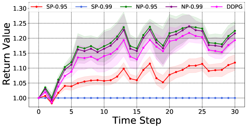
(a)

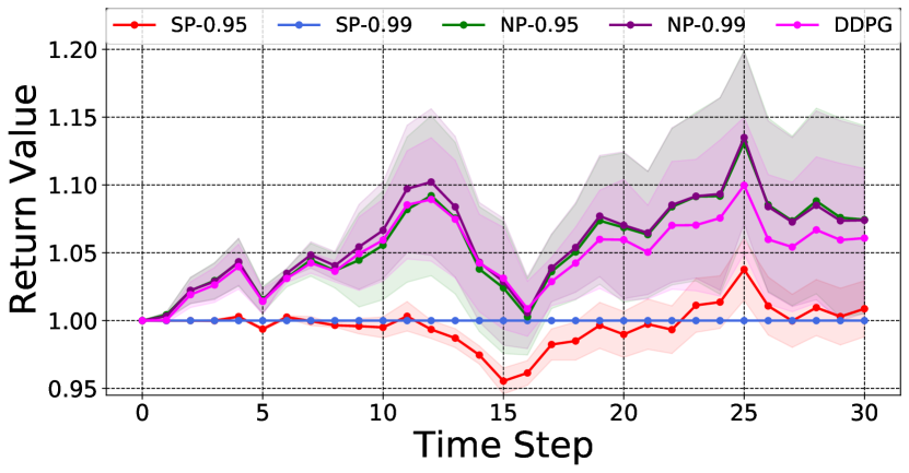
(b)

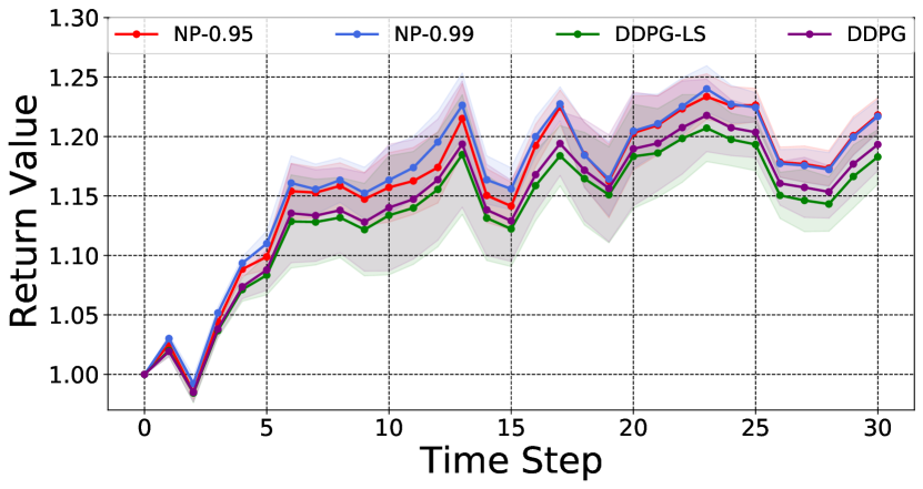
(c)

Figure 1: (a)–(b) Returns without liquidity constraints. NP policies outperform DDPG, SP; (c) Sample efficiency of NP.

	First 30 days, annualized values				Second 30 days, annualized values
Algorithms	Returns	Sharpe	Volatility	MDD	Returns	Sharpe	Volatility	MDD
SP-0.0	11.84	3.58	27.33	7.63	2.3	1.16	17.8	4.8
SP-0.95	11.83	3.58	27.37	7.65	0.87	0.51	17.32	4.85
SP-0.99	0.0	-0.54	0.0	0.0	0.0	-3.78	0.0	0.0
NP-0.0	22.47	4.44	40.29	10.46	7.44	2.22	29.1	7.41
NP-0.95	22.47	4.44	40.29	10.46	7.44	2.22	29.1	7.41
NP-0.99	21.64	4.29	40.38	10.44	7.4	2.09	30.96	7.99
DDPG	19.33	4.36	35.63	9.52	6.08	2.12	24.86	5.93
uCRP	12.08	5.68	17.16	5.26	1.38	0.97	12.5	3.77
OLMAR	10.4	4.65	18.26	5.97	-4.17	-2.69	12.98	3.54
PAMR	6.35	2.45	22.08	6.03	-8.02	-3.39	20.1	5.19
RMR	10.68	4.72	18.45	5.97	-4.56	-2.82	13.58	3.83

Table 1: Performance without liquidity constraints. NP policies nearly always outperform all other strategies. SP with $\alpha=0.99$ puts all funds in cash, hence MDD and volatility are 0, but returns are 0 as well.

(a)

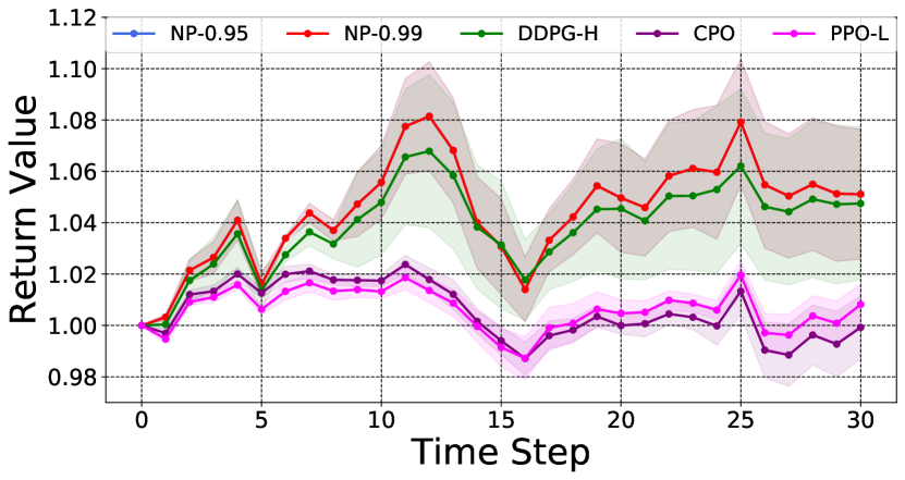
(b)

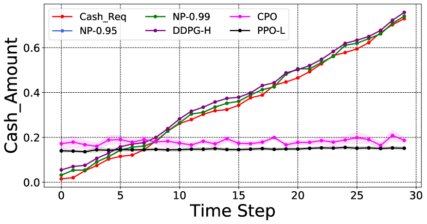
(c)

Figure 2: (a)-(b) Returns with liquidity constraints. NP with CVaR_α=95 and CVaR_α=99 are nearly identical in (b). NP policies outperform CPO, PPO-L and DDPG-H; (c) Average liquidity in each policy, Liquidity constraint is shown in red.

A significant benefit of the NP framework is the ability to enforce constraints, otherwise difficult to handle in an RL policy. Figure 2(a)-(b) show the mean and standard error in returns under liquidity constraints. We compare against a heuristic we call DDPG-H that uses DDPG, but reserves $\mu_{\ell}+3\sigma_{\ell}$ of the funds for the 0-interest cash account by re-normalizing the remaining allocations. DDPG-H thus provides a conservative, but constraint-feasible policy, by construction. The constrained NP policy outperforms CPO, PPO-L, DDPG-H and even the unconstrained DDPG policy. In Figure 2(c), we show constraint violations; the red increasing line shows cumulative liquidity demand in each period. Although PPO-L, unlike CPO, was able to learn the constraints during training (see Appendix A.2 for constraint violations during training), both CPO and PPO-L are unable to come close to satisfying the liquidity constraints in testing. Only DDPG-H and NP satisfy the constraints in testing, but the DDPG-H method over-allocates to the liquid account, thereby reducing net returns.

4.2 Online repositioning in bike-sharing systems

The bike repositioning problem is a form of online resource matching in an uncertain environment. Uncoordinated movements of users in bike or electric vehicle sharing, along with demand uncertainty, results in the need to often reposition the resources [Ghosh et al., 2017, Schuijbroek et al., 2017, Ghosh et al., 2016, Ghosh and Varakantham, 2017]. We use an RL-based simulator from Bhatia et al. [2019] built upon the dataset of Hubway bike sharing system in Boston, consisting of 95 base stations and 760 bikes. The state at time $t$ includes the current allocated bikes in each station $j\in\{1\ldots J\}$ and $\xi_{t,j}$ is the random customer demand at station $j$. The action is a vector, $x_{t}=\{x_{t,1},...,x_{t,J}\},$ that represents the percent allocations of bikes across all stations while respecting the constraint set $\mathcal{G}(\xi):=\{x|\check{C}_{j}\leq N\cdot x_{t,j}\leq\hat{C}_{j},\sum_{j}x_{t,j}=1,t=1\ldots T\}$, where $\check{C}_{j}$ and $\hat{C}_{j}$ denote the minimum and maximum bounds on the number of allocated bikes at station $j$, and $N$ denotes the total number of bikes present in the system. The objective function is represented by:

$$\max_{x}\!\sum_{t}\!\sum_{j}\! -L(x_{t,j},\xi)(1+\log(1+L(x_{t,j},\xi))-R(x_{t,j},\xi)\sin(\pi\cdot R(x_{t,j},\xi))$$

where $L(x_{t,j},\xi)$ represents the amount of unfulfilled demand and $R(x_{t,j},\xi)$ is the number of bikes picked up or dropped off at station $j$ at time $t$ in action $x$, which incurs a repositioning cost. We use two months of data to train the models. We evaluate the learnt policies on 3 consecutive days during the morning peak period (6AM–12PM) with 12 decision epochs, each having a duration of 30 minutes.

Figure 3(a) shows mean and standard error in cumulative reward over 3 test days from NP with CVaR of $\alpha=0.0,0.99$, CPO and PPO-L, and unconstrained DDPG. After training CPO and PPO-L methods for 1 million episodes, they fail to perform at par with NP. NP using expected reward (i.e., $\alpha=0.0$) and with CVAR of $\alpha=0.99$ improves cumulative reward by 11.3% and 7.9% over unconstrained DDPG. Figure 3(b) shows the cumulative constraint violation where capacity violation per station costs 1 unit. Only NP variants satisfy the constraints, while both CPO and PPO-L fail to satisfy the capacity constraints during the test period.

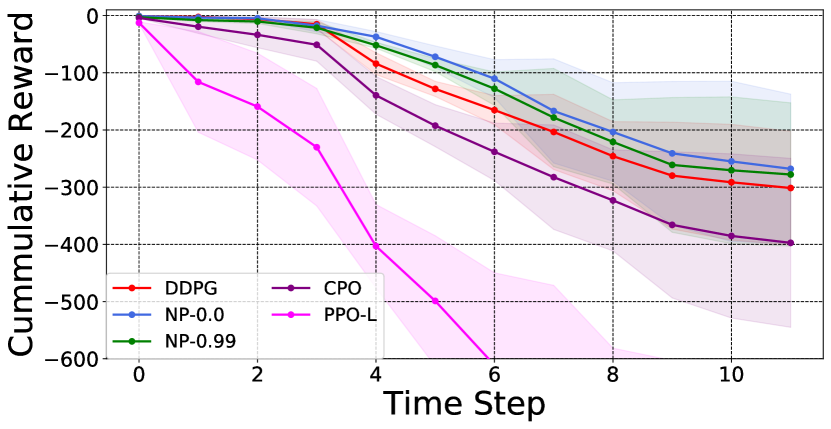
(a)

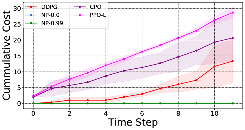
(b)

Figure 3: Performance comparison on the online bike repositioning problem for 12 time steps (6AM-12PM), averaged over 3 testing days: (a) cumulative reward value; (b) cumulative constraint violation cost.

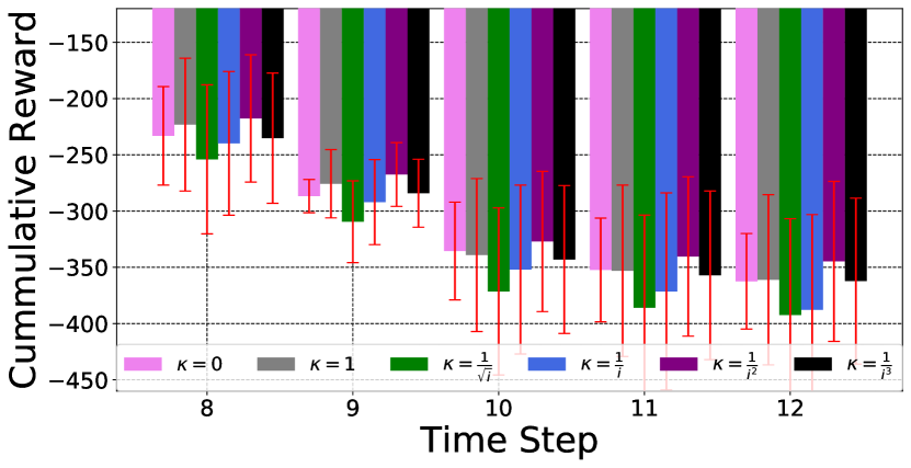
(a)

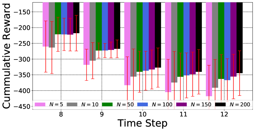
(b)

Figure 4: Sensitivity analysis results by varying (a) convex combination parameter, $\kappa$; and (b) number of scenarios.

Finally, we provide sensitivity analysis by varying (a) convex combination parameter, $\kappa$; and (b) number of scenarios sampled from the demand distribution. Figure 4(a) shows the mean and standard error in cumulative reward for different $\kappa$ that decreases over iterations of NP. Recall that at $\kappa=1$ and $0$, NP reduces to DDPG and pure SP, respectively. The best performance is achieved with $\kappa=\frac{1}{i^{2}}$, which is our default setting in the experiments. Figure 4(b) shows the cumulative reward of NP in the last five time steps, varying the number of scenarios. NP performance improves with the number of scenarios, but in a concave manner. We thus use 200 scenarios for both the pure SP and NP in the experiments.

5 Related work

The neural-progressive hedging algorithm combines offline policy search with an online model-based phase to fine-tune the policy so as to satisfy constraints and risk measures such as CVaR. We categorize the existing relevant research into three threads: (a) Combining model-free and model-based methods for performance improvement; (b) Constrained and risk-sensitive RL methods; and (c) Improving sequential decisions through warm starting and imitation learning.

Ensemble of model-free and model-based methods: Model-based methods are prized for sample efficiency, but, as noted by Feinberg et al. [2018], high-capacity models are “prone to over-fitting in the low-data regimes where they are most needed", implying that the combination of model-based and model-free methods will be important for good performance in complex settings. They propose, as do Buckman et al. [2018], to rollout the learned model for use in value estimation of a model-free RL, in the latter reference using an ensemble of such models to estimate variance. Lu et al. [2019], Amos et al. [2018], Tamar et al. [2017], Kahn et al. [2017] combine (online) planning models with model-free RL to explore more sparingly the state and action spaces. Amos et al. [2018] propose to differentiate through a planning model using analytical expressions for the derivatives of a convex approximation of a non-convex model. Mansard et al. [2018] suggest a structure similar to ours for controlling dynamical systems using models to initialize a model predictive control formulation, as a warm-start. Lu et al. [2019] develop Adaptive Online Planning (AOP) with a continuous model-free RL algorithm, TF3 [Fujimoto et al., 2018]. The goal is similar to ours – leveraging the responsiveness of online planning with reactive off-policy learning to make better decisions. The approach is however different from ours – AOP uses a model-based policy when uncertainty is high and a reactive model-free policy when habitual behavior should suffice.

Constrained and risk-sensitive RL methods: Garcıa and Fernández [2015] surveyed safe RL methods which they classify as either optimization-based or handling safety in the exploration process. Pham et al. [2018] suggest after each policy update to project the current iterate onto the feasible set of safety constraints; since they assume that the safety constraints may not be known in advance, they propose a method to learn the parameters of a linear polytope. Yang et al. [2019] extend CPO method to solve constrained RL by optimizing the reward function using TRPO and then projecting the solution onto the feasible region defined by safety constraints, similar to Pham et al. [2018]. Chow et al. [2015, 2017] model risk-constrained MDPs with a CVaR objective or chance constraints, and solve it by relaxing the constraints and using a policy gradient algorithm. However, similar to CPO and Lagrangian-relaxed PPO, the constraints are not enforced during execution and need not be satisfied. Most “safe" RL methods use an initial infeasible, unconstrained policy and iteratively render it feasible and locally optimal, e.g., Berkenkamp et al. [2017] define an expanding “region of attraction" to guide safe exploration to improve the policy, whilst remaining feasible.

Imitation learning and warm start: NP can be viewed through the lens of imitation learning. Gu et al. [2016] use synthetic model-based “imagination" rollouts in the early iterations of deep RL training, which can be considered as a model-based warm-start. This is the opposite of our approach, we propose a longer-horizon deep RL to warm start the online stochastic program. Aggravate [Ross and Bagnell, 2014] and Aggravated [Sun et al., 2017], building on the seminal DAgger [Ross et al., 2011], involve iteratively mixing the learning step of a policy with an expert policy, in that, at iteration $n$, $\pi^{n}=\beta^{n}\pi^{*}+(1-\beta^{n})\hat{\pi}^{n}$, where $\beta\rightarrow 0$ as $n\rightarrow\infty$. This is similar to the update step of NP which uses a convex combination of the expert and the learner policies, with damping. Cheng et al. [2018] take this one step further by defining a framework with a mirror descent gradient update that reduces to imitation learning-based RL, depending on the choice of the gradient estimator; they introduce SLOLS, where the gradient is a convex combination of a policy gradient and an expert gradient. Sun et al. [2018] propose combining imitation learning and RL with the aim of faster learning and improving beyond a sub-optimal expert. The advantages achieved by the NP method in inverting the roles of expert and learner are the ability of the SP to enforce hard constraints and incorporate risk measures, and doing so in an explainable manner. The NP warm start serves as an external expert to guide the SP in the early iterations to encourage convergence to a better solution by reshaping the objective itself.

6 Conclusion

The neural-progressive hedging (NP) method starts from an offline, unconstrained RL policy and iteratively enforces constraints and risk requirements using model-based stochastic programming. The framework is thus a type of external point method. We demonstrate the efficacy of NP method on two real-world applications, in finance and logistics. The NP method significantly outperforms both constrained and unconstrained RL whilst handling both resource constraints and risk measures. An important benefit of the framework is its ease of implementation: NP method can be implemented using existing deep RL algorithms and commercial off-the-shelf optimization packages, and provides added transparency and explainability on the constraint satisfaction of the policy.

Appendix

Appendix A Additional Numerical Results

In this section, we provide additional empirical results on the convergence of NP method, the effect of warm-starting NP with an offline RL solution, and episodic constraint violation cost for CPO and PPO-L benchmarks during the training process.

A.1 Convergence and effect of warm-starting

Figure 5(a) shows the convergence of the NP method, in the presence of and after damping to zero the expert guidance. According to Theorem 1, initial iterates may decrease non-monotonically but for iterations $i\geq\hat{\imath}=20$ progression to an optimum is monotonic Figure 5(b) compares the warm-start (called NP-WS) version with the damped-guidance, or imitation-learning-type expert guidance (called NP). Both warm-starting and imitation learning with damping for CVaR $\alpha=0.95$ and $0.99$ perform far better than the baseline DDPG policy.

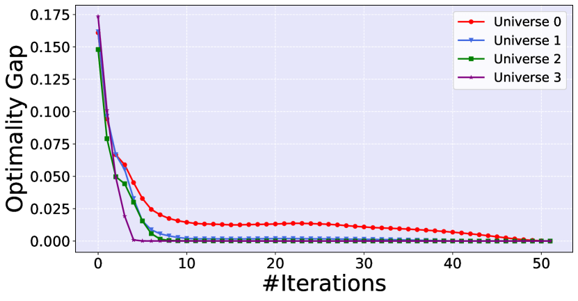
(a)

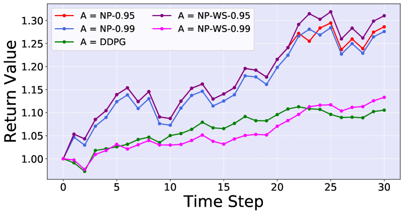
(b)

Figure 5: (a) Convergence of the neural-progressive hedging algorithm with CVaR_α=95; (b) Performance comparison of two versions of the algorithm: warm start ($\kappa^{1}=1$, $\hat{\imath}=1$) vs. imitation learning ($\kappa^{i}=(1+i)^{-2}$, $\hat{\imath}=20$, in this example).

A.2 Constraint violation for benchmark constrained RL

Figure 6 illustrates the episodic constraint violation cost for two benchmark constrained RL algorithms, CPO of Achiam et al. [2017], and PPO-Lagrangian of Ray et al. [2019], for the financial planning domain. Each episode duration is 30 time steps and in each time step $t$, we enforce a cost of 1 if the amount available in the liquid instrument is less than the cumulative account payable up through time $t$. Observe that CPO fails to learn the constraints during training. The PPO-Lagrangian method is able to bring down the episodic cost to 0 during training (the limit of the episodic cost is set to 0), but as shown in the main paper (see Figure 2(c)), the learned PPO-L policy is not able to satisfy the constraints during execution.

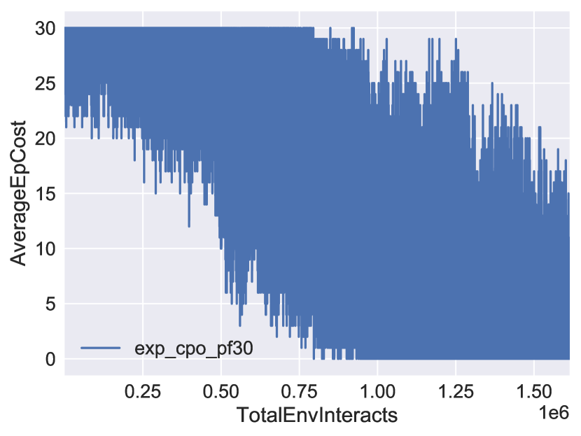
(a)

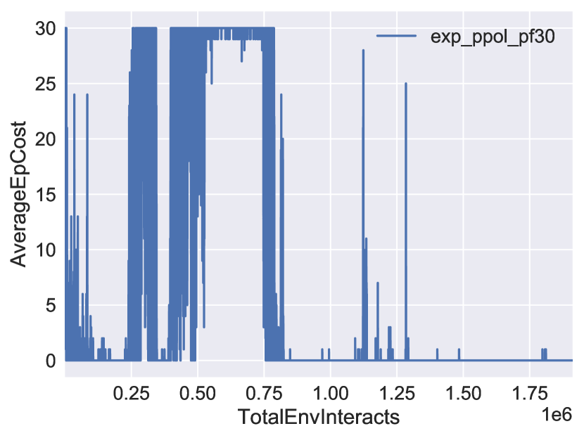
(b)

Figure 6: Episodic (episode length = 30) constraint violation cost during training for (a) CPO; and (b) PPO-Lagrangian.

Appendix B Additional Implementation Details

Discretization of the stochastic program scenario tree:

Consider a finite scenario tree formulation of a stochastic programming problem, such that the set of nodes in the scenario tree at time stage $t$ are denoted $N_{t}$. A node denotes a point in time when a realisation of the random process becomes known and a decision is taken. Each node replicates the data of the optimization problem, conditioned on the probability of visiting that node from its parent node. A path from the root to each leaf node is referred to as a scenario; its probability of occurrence, $p_{s}$, is the product of the conditional probabilities of visiting each of the nodes on that scenario path. The discretized model-based stochastic program is thus:

$$\max\sum_{s=1\ldots S}F_{s}(x,\xi):=\sum_{s=1\ldots S}p_{s}\sum_{t=1\ldots T}f_{t}(x_{s}(t)).$$ (8)

The non-anticipativity constraints are critical for the implementability of the policy but they couple the scenario sub-problems by requiring that the action $x_{t}$ at time $t$ is the same across scenarios (i.e., sample paths) sharing the sample path up to and including time $t$. For each $\xi\in\Xi$, these coupling constraints are expressed as:

$$x(\xi)=(x_{1},x_{2}(\xi_{1}),x_{3}(\xi_{1},\xi_{2}),\ldots x_{T}(\xi_{1}\ldots\xi_{T-1}).$$ (9)

Using the discretized formulation of (8), and following Rosa and Ruszczyński [1996] we can rewrite (9) in a manner that facilitates relaxation of those constraints: Define the last common stage of two scenarios $s_{1}$ and $s_{2}$ as

$$t^{\max}(s_{1},s_{2}):=\max\{\hat{t}:s_{1}(t)=s_{2}(t),t=1,\ldots\hat{t}\},$$ (10)

and then re-order the scenarios $s=1\ldots S$, so that at every $s$, the scenario $s+1$ has the largest common stage with scenario $i$ for all scenarios $s^{\prime}>s$, that is $t^{\max}(s,s+1):=\max\{t^{\max}(u,v):v>u\}$. Then, define the sibling of scenario $s$ at time stage $t$ as a permutation $\nu(s,t):=s+1$ if $t_{\max}(s,s+1)\geq t$ and $\nu(s,t):=\min\{t^{\prime}:t^{\max}(s,t^{\prime})\geq t\}$ otherwise. The inverse permutation shall be denoted $\nu^{-1}(s,t).$ Note that the sibling of a scenario depends upon the time stage, and that a scenario with no shared decisions at a time stage has by definition itself as sibling. Using the above, Rosa and Ruszczyński [1996] re-define the constraints enforcing measurability in terms of the sibling function as follows:

$$x_{s}(t)=x_{\nu(s,t)}(t)\;\;\forall(s,t),\;s\neq\nu(s,t).$$ (11)

Equation (11) is convenient in the primal-dual formulation in terms of discrete scenarios, presented next. We are interested in maintaining the separability of the subproblems which depend only on individual scenarios of the random variable to facilitate handling large problems via scenario-based decomposition. To do so, we relax the constraints using the following formulation

$$\mathcal{M}:=\{x:M_{1}x_{1}(\xi)+\ldots+M_{S}x_{S}(\xi)=0\},$$ (12)

where the matrices in (12) are defined so that each $M_{s}$ is a matrix of -1, 0 and 1 such that at the root node $x_{11}=x_{12},x_{12}=x_{23}=\cdots x_{1,s-1}=x_{1,s}$, at the stage $t=2$, there are as many such sets of equalities as children nodes emanating from the root node, and so on up to stage $T-1$. At stage $T$, all nodes are leaves and no such linking constraints are required. The projection of a point $x^{i}$ onto the subspace $\mathcal{M}$, $P_{\mathcal{M}}[x^{i}(\cdot)]$ can be computed by taking the conditional expectation of $x^{i}$, $E_{\xi\,|\,\xi_{1},\ldots\xi_{i-1}}$. Lagrange relaxation of the measurability constraints (11) gives rise to the following Lagrange function, in terms of the discrete scenarios $s=1\ldots S$:

$$\mathcal{L}(x,\lambda)=\sum_{s=1\ldots S}p_{s}\sum_{t=1\ldots T}f_{t}(x_{s}(t))+\sum_{s=1\ldots S}\sum_{t=1\ldots T-1}\lambda_{s}(t)(x_{s}(t)-x_{\nu(s,t)}(t)).$$ (13)

The scenario subproblems are re-defined as a function of the inverse permutation of the sibling function:

$$\min_{x_{s}\in G^{\prime}_{s}}\mathcal{L}_{s}(x_{s},\lambda_{s})=p_{s}\sum_{t=1\ldots T}f_{t}(x_{s}(t))+\sum_{t=1\ldots T-1}(\lambda_{s}(t)-\lambda_{\nu^{-1}(s,t)}(t))x_{s}(t)$$ (14)

for each $s=1\ldots S$. The dual problem is given by

$$\max_{\lambda}D(\lambda):=\min_{x\in G^{\prime}}\mathcal{L}(x,\lambda).$$ (15)

It is possible to further speed up convergence of our NP algorithm in practice using the approach of Zehtabian and Bastin [2016]. This approach monitors the primal and dual gap terms in convergence criteria separately to update the penalty parameters so as to reduce the convergence gap quickly.

References

- Achiam et al. [2017] Joshua Achiam, David Held, Aviv Tamar, and Pieter Abbeel. Constrained policy optimization. In Proceedings of the 34th International Conference on Machine Learning, pages 22–31. JMLR. org, 2017.
- Altman [1999] Eitan Altman. Constrained Markov decision processes, volume 7. CRC Press, 1999.
- Amos et al. [2018] Brandon Amos, Ivan Jimenez, Jacob Sacks, Byron Boots, and J Zico Kolter. Differentiable mpc for end-to-end planning and control. In Advances in Neural Information Processing Systems, pages 8289–8300, 2018.
- Berkenkamp et al. [2017] Felix Berkenkamp, Matteo Turchetta, Angela P Schoellig, and Andreas Krause. Safe model-based reinforcement learning with stability guarantees. In International Conference on Neural Information Processing Systems, pages 908–919, 2017.
- Bertsimas et al. [2018] Dimitris Bertsimas, Vishal Gupta, and Nathan Kallus. Robust sample average approximation. Mathematical Programming, 171(1-2):217–282, 2018.
- Bhatia et al. [2019] Abhinav Bhatia, Pradeep Varakantham, and Akshat Kumar. Resource constrained deep reinforcement learning. In International Conference on Automated Planning and Scheduling, volume 29, pages 610–620, 2019.
- Buckman et al. [2018] Jacob Buckman, Danijar Hafner, George Tucker, Eugene Brevdo, and Honglak Lee. Sample-efficient reinforcement learning with stochastic ensemble value expansion. In Advances in Neural Information Processing Systems, pages 8224–8234, 2018.
- Cheng et al. [2018] Ching-An Cheng, Xinyan Yan, Nolan Wagener, and Byron Boots. Fast policy learning through imitation and reinforcement. arXiv preprint arXiv:1805.10413, 2018.
- Chow et al. [2015] Yinlam Chow, Aviv Tamar, Shie Mannor, and Marco Pavone. Risk-sensitive and robust decision-making: a cvar optimization approach. In Proceedings of the 28th International Conference on Neural Information Processing Systems, pages 1522–1530, 2015.
- Chow et al. [2017] Yinlam Chow, Mohammad Ghavamzadeh, Lucas Janson, and Marco Pavone. Risk-constrained reinforcement learning with percentile risk criteria. The Journal of Machine Learning Research, 18(1):6070–6120, 2017.
- Cover [2011] Thomas M Cover. Universal portfolios. In The Kelly Capital Growth Investment Criterion: Theory and Practice, pages 181–209. World Scientific, 2011.
- Feinberg et al. [2018] Vladimir Feinberg, Alvin Wan, Ion Stoica, Michael I Jordan, Joseph E Gonzalez, and Sergey Levine. Model-based value estimation for efficient model-free reinforcement learning. arXiv preprint arXiv:1803.00101, 2018.
- Fujimoto et al. [2018] Scott Fujimoto, Herke Van Hoof, and David Meger. Addressing function approximation error in actor-critic methods. arXiv preprint arXiv:1802.09477, 2018.
- Garcıa and Fernández [2015] Javier Garcıa and Fernando Fernández. A comprehensive survey on safe reinforcement learning. Journal of Machine Learning Research, 16(1):1437–1480, 2015.
- Ghosh and Varakantham [2017] Supriyo Ghosh and Pradeep Varakantham. Incentivizing the use of bike trailers for dynamic repositioning in bike sharing systems. In Proceedings of the International Conference on Automated Planning and Scheduling, volume 27, 2017.
- Ghosh et al. [2016] Supriyo Ghosh, Michael Trick, and Pradeep Varakantham. Robust repositioning to counter unpredictable demand in bike sharing systems. International Joint Conference on Artificial Intelligence (IJCAI), 2016.
- Ghosh et al. [2017] Supriyo Ghosh, Pradeep Varakantham, Yossiri Adulyasak, and Patrick Jaillet. Dynamic repositioning to reduce lost demand in bike sharing systems. Journal of Artificial Intelligence Research, 58:387–430, 2017.
- Ghosh et al. [2019] Supriyo Ghosh, Jing Yu Koh, and Patrick Jaillet. Improving customer satisfaction in bike sharing systems through dynamic repositioning. In International Joint Conferences on Artificial Intelligence (IJCAI), 2019.
- Gu et al. [2016] Shixiang Gu, Timothy Lillicrap, Ilya Sutskever, and Sergey Levine. Continuous deep q-learning with model-based acceleration. In International Conference on Machine Learning, pages 2829–2838, 2016.
- Huang et al. [2016] Dingjiang Huang, Junlong Zhou, Bin Li, Steven CH Hoi, and Shuigeng Zhou. Robust median reversion strategy for online portfolio selection. IEEE Transactions on Knowledge and Data Engineering, 28(9):2480–2493, 2016.
- Kahn et al. [2017] Gregory Kahn, Tianhao Zhang, Sergey Levine, and Pieter Abbeel. Plato: Policy learning using adaptive trajectory optimization. In 2017 IEEE International Conference on Robotics and Automation (ICRA), pages 3342–3349. IEEE, 2017.
- Li and Hoi [2012] Bin Li and Steven CH Hoi. On-line portfolio selection with moving average reversion. arXiv preprint arXiv:1206.4626, 2012.
- Li et al. [2012] Bin Li, Peilin Zhao, Steven CH Hoi, and Vivekanand Gopalkrishnan. Pamr: Passive aggressive mean reversion strategy for portfolio selection. Machine learning, 87(2):221–258, 2012.
- Liang et al. [2017] Eric Liang, Richard Liaw, Robert Nishihara, Philipp Moritz, Roy Fox, Joseph Gonzalez, Ken Goldberg, and Ion Stoica. Ray rllib: A composable and scalable reinforcement learning library. arXiv preprint arXiv:1712.09381, 2017.
- Lillicrap et al. [2015] Timothy P Lillicrap, Jonathan J Hunt, Alexander Pritzel, Nicolas Heess, Tom Erez, Yuval Tassa, David Silver, and Daan Wierstra. Continuous control with deep reinforcement learning. arXiv preprint arXiv:1509.02971, 2015.
- Lu et al. [2019] Kevin Lu, Igor Mordatch, and Pieter Abbeel. Adaptive online planning for continual lifelong learning. arXiv preprint arXiv:1912.01188, 2019.
- Mansard et al. [2018] Nicolas Mansard, Andrea DelPrete, Mathieu Geisert, Steve Tonneau, and Olivier Stasse. Using a memory of motion to efficiently warm-start a nonlinear predictive controller. In 2018 IEEE International Conference on Robotics and Automation (ICRA), pages 2986–2993. IEEE, 2018.
- Mnih et al. [2013] Volodymyr Mnih, Koray Kavukcuoglu, David Silver, Alex Graves, Ioannis Antonoglou, Daan Wierstra, and Martin Riedmiller. Playing atari with deep reinforcement learning. arXiv preprint arXiv:1312.5602, 2013.
- Pham et al. [2018] Tu-Hoa Pham, Giovanni De Magistris, and Ryuki Tachibana. Optlayer-practical constrained optimization for deep reinforcement learning in the real world. In 2018 IEEE International Conference on Robotics and Automation (ICRA), pages 6236–6243. IEEE, 2018.
- Ray et al. [2019] Alex Ray, Joshua Achiam, and Dario Amodei. Benchmarking safe exploration in deep reinforcement learning. Technical report, Open AI, 2019.
- Rockafellar [2018] R. Tyrrell Rockafellar. Solving stochastic programming problems with risk measures by progressive hedging. Set-Valued and Variational Analysis, 26:759–768, 2018.
- Rockafellar [2019] R Tyrrell Rockafellar. Progressive decoupling of linkages in optimization and variational inequalities with elicitable convexity or monotonicity. Set-Valued and Variational Analysis, 27(4):863–893, 2019.
- Rockafellar and Wets [1991] R Tyrrell Rockafellar and Roger J-B Wets. Scenarios and policy aggregation in optimization under uncertainty. Mathematics of operations research, 16(1):119–147, 1991.
- Rosa and Ruszczyński [1996] Charles H Rosa and Andrzej Ruszczyński. On augmented lagrangian decomposition methods for multistage stochastic programs. Annals of Operations Research, 64(1):289–309, 1996.
- Ross and Bagnell [2014] Stephane Ross and J Andrew Bagnell. Reinforcement and imitation learning via interactive no-regret learning. arXiv preprint arXiv:1406.5979, 2014.
- Ross et al. [2011] Stéphane Ross, Geoffrey Gordon, and Drew Bagnell. A reduction of imitation learning and structured prediction to no-regret online learning. In Proceedings of the fourteenth international conference on artificial intelligence and statistics, pages 627–635, 2011.
- Schuijbroek et al. [2017] Jasper Schuijbroek, Robert C Hampshire, and W-J Van Hoeve. Inventory rebalancing and vehicle routing in bike sharing systems. European Journal of Operational Research, 257(3):992–1004, 2017.
- Schulman et al. [2015] John Schulman, Sergey Levine, Pieter Abbeel, Michael Jordan, and Philipp Moritz. Trust region policy optimization. In International conference on machine learning, pages 1889–1897, 2015.
- Schulman et al. [2017] John Schulman, Filip Wolski, Prafulla Dhariwal, Alec Radford, and Oleg Klimov. Proximal policy optimization algorithms. arXiv preprint arXiv:1707.06347, 2017.
- Silver et al. [2017] David Silver, Julian Schrittwieser, Karen Simonyan, Ioannis Antonoglou, Aja Huang, Arthur Guez, Thomas Hubert, Lucas Baker, Matthew Lai, Adrian Bolton, et al. Mastering the game of go without human knowledge. Nature, 550(7676):354–359, 2017.
- Sun et al. [2017] Wen Sun, Arun Venkatraman, Geoffrey J Gordon, Byron Boots, and J Andrew Bagnell. Deeply aggrevated: Differentiable imitation learning for sequential prediction. In Proceedings of the 34th International Conference on Machine Learning, pages 3309–3318. JMLR. org, 2017.
- Sun et al. [2018] Wen Sun, J Andrew Bagnell, and Byron Boots. Truncated horizon policy search: Deep combination of reinforcement and imitation. In International Conference on Learning Representations, 2018.
- Tamar et al. [2017] Aviv Tamar, Garrett Thomas, Tianhao Zhang, Sergey Levine, and Pieter Abbeel. Learning from the hindsight plan—episodic mpc improvement. In 2017 IEEE International Conference on Robotics and Automation (ICRA), pages 336–343. IEEE, 2017.
- Wächter and Biegler [2006] Andreas Wächter and Lorenz T Biegler. On the implementation of an interior-point filter line-search algorithm for large-scale nonlinear programming. Mathematical programming, 106(1):25–57, 2006.
- Yang et al. [2019] Tsung-Yen Yang, Justinian Rosca, Karthik Narasimhan, and Peter J Ramadge. Projection-based constrained policy optimization. In International Conference on Learning Representations, 2019.
- Zehtabian and Bastin [2016] Shohre Zehtabian and Fabian Bastin. Penalty parameter update strategies in progressive hedging algorithm. CIRRELT, 2016.